A Hybrid Radial Basis Function - Pseudospectral Method for

Thermal Convection in a 3D Spherical Shell∗

Grady B. Wright †

Department of Mathematics

Boise State University

Boise, ID 83725

Natasha Flyer

Institute for Mathematics Applied to Geosciences

National Center for Atmospheric Research

Boulder, CO 80305 USA

David A. Yuen

Department of Geology and Geophysics

University of Minnesota

Minneapolis, MN 55455

May 13, 2010

Abstract

A novel hybrid spectral method that combines radial basis function (RBF) and Chebyshevpseudospectral (PS) methods in a “2+1” approach is presented for numerically simulating ther-mal convection in a 3D spherical shell. This is the first study to apply RBFs to a full 3Dphysical model in spherical geometry. In addition to being spectrally accurate, RBFs are notdefined in terms of any surface based coordinate system such as spherical coordinates. As aresult, when used in the lateral directions, as in this study, they completely circumvent the poleissue with the further advantage that nodes can be “scattered” over the surface of a sphere. Inthe radial direction, Chebyshev polynomials are used, which are also spectrally accurate andprovide the necessary clustering near the boundaries to resolve boundary layers. Applicationsof this new hybrid methodology are given to the problem of convection in the Earth’s mantle,which is modeled by a Boussinesq fluid at infinite Prandtl number. To see whether this nu-merical technique warrants further investigation, the study limits itself to an isoviscous mantle.Benchmark comparisons are presented with other currently used mantle convection codes forRayleigh number (Ra) 7 · 103 and 105. Results from a Ra = 106 simulation are also given. Thealgorithmic simplicity of the code (mostly due to RBFs) allows it to be written in less than 400lines of Matlab and run on a single workstation. We find that our method is very competitivewith those currently used in the literature.

∗Accepted for publication in Geochem. Geophys. Geosyst., 2010†Corresponding author; wright@math.boisestate.edu.

1

1 Introduction

Mantle convection models in spherical geometry have seen a variety of numerical method imple-mentations, from finite element and finite volume methods on a variety of grids such as icosahedral,cubed-sphere, Ying-Yang, spiral, and hexahedral [Baumgardner, 1985; Hernlund and Tackley, 2003;Yoshida and Kageyama, 2004; Harder and Hansen, 2005; Stemmer et al., 2006; Huettig and Stem-mer, 2008; Zhong et al., 2000, 2008], to pseudospectral methods using spherical harmonics [Bercoviciet al., 1989; Harder, 1998]. The former methods can be cumbersome and tedious to program dueto grid generation and treatment of the equations near element boundaries and are generally loworder. The latter requires more nodes than basis functions (especially when dealiasing filters areused), since there are 2N + 1 longitudinal Fourier modes for each latitudinal associated Legendrefunction of degree N , and does not easily allow for local refinement.

A novel approach that is in its infancy of development is radial basis functions (RBFs), a mesh-less method that has the advantage of being spectrally accurate for arbitrary node layouts inmulti-dimensions. Former studies, using this method on spherical surfaces, have shown it to bevery competitive in comparison to numerical methods that are currently used in the geosciences,algorithmically simpler, and naturally permitting local node refinement [Flyer and Wright, 2009;Flyer and Lehto, 2009; Flyer and Wright, 2007; Fornberg and Piret, 2008]. However, given thisearly stage of development, numerical modeling experiments with RBFs are warranted before full-blown mantle convection models using RBFs are developed that can handle everything from variableviscosity to thermochemical convection. As a result, this paper is of an exploratory nature from theperspective of numerics. Since no 3D model using RBF spatial discretization of partial differentialequations (PDEs) in spherical geometry exists in the math or science literature, it follows that takingthe simplest formulation for mantle convection, isoviscous flows at various Rayleigh numbers (as isdone by Bercovici et al. [1989] and Harder [1998]) would be a good starting point.

The paper is organized as follows: Section 2 describes the physical model; Section 3 gives anintroduction to RBFs; Section 4 shows how the spatial operators are discretized using RBFs;Section 5 reviews the concept of influence matrices that must be used for solving the coupled Poissonequations which result from writing the velocity in terms of a poloidal potential [see Chandrasekhar,1961]; Section 6 describes the time discretization; Section 7 provides numerical results from twotest cases with comparisons to those in the literature and results from a Ra = 106 simulation;Section 8 gives timing results for the benchmark cases and Section 9 discusses extensions of themethod to high Ra, variable viscosity, and local node refinement. The appendices give the stepsfor implementing the RBF-PS algorithm.

2 The Physical Model

We consider a thermal convection model of a Boussinesq fluid at infinite Prandtl number in aspherical shell that is heated from below. The governing equations are

∇ · u = 0 (continuity), (1)

∇ ·[η

(∇u + ∇uT

)]+ RaT r = ∇p (momentum), (2)

∂T

∂t+ u · ∇T = ∇2T (energy), (3)

where u = (ur, uθ, uλ) is the velocity field in spherical coordinates (θ=latitude, λ=longitude), p ispressure, T is temperature, r is the unit vector in the radial direction, η is the viscosity, and Ra is

2

the Rayleigh number. The boundary conditions on the velocity of the fluid at the inner and outersurfaces of the spherical shell are

ur|r=Ri,Ro= 0

︸ ︷︷ ︸impermeable

and r∂

∂r

(uθ

r

)∣∣∣∣r=Ri,Ro

= r∂

∂r

(uλ

r

)∣∣∣∣r=Ri,Ro

= 0

︸ ︷︷ ︸shear-stress free

, (4)

where Ri is the radius of the inner surface of the shell and Ro is the radius of the outer surface asmeasured from the center of the earth. The boundary conditions on the temperature are

T (Ri, θ, λ) = 1 and T (Ro, θ, λ) = 0.

Equations (1)-(3) have been non-dimensionalized with the length scale chosen as the thickness of theshell, ∆R = Ro−Ri, the time-scale chosen as the thermal diffusion time, t = (∆R)2/κ (κ=thermaldiffusivity), and the temperature scale chosen as the difference between the temperature at theinner and outer boundaries, ∆T .

In this study, we treat the fluid as isoviscous, η =const. Thus, the dynamics of the fluid are governedby the Ra, which can be interpreted as a ratio of the destabilizing force due to the buoyancy of theheated fluid to the stabilizing force due to the viscosity of the fluid. It takes the specific form of

Ra =ρgα∆T (∆R)3

κη,

where ρ is the density of the fluid, g is the acceleration due to gravity, and α is the coefficient ofthermal expansion.

Chandrasekhar [1961] [see also Backus, 1966] shows that any divergence-free field can be expressedin terms of a poloidal and toroidal potential, u = ∇ × ∇ × ((Φr)r) + ∇ × (Ψr). If the fluid isisoviscous (or the viscosity stress tensor is spherically symmetric) and satisfies (4) then the fieldis purely poloidal (i.e. Ψ ≡ 0). As a result, the three-dimensional continuity and momentumequations (1) and (2) can be alternatively written as a system of two coupled Poisson equations.The nonlinear thermal convection model can then be written as

∆sΩ +∂

∂r

(r2 ∂Ω

∂r

)= Ra r T, (5)

∆sΦ +∂

∂r

(r2 ∂Φ

∂r

)= r2Ω, (6)

∂T

∂t= −

(ur

∂T

∂r+ uθ

1

r

∂T

∂θ+ uλ

1

r cos θ

∂T

∂λ

)+

1

r2∆sT +

1

r2

∂

∂r

(r2 ∂T

∂r

), (7)

where θ ∈ [−π/2, π/2], λ ∈ (−π, π], and ∆s is the surface Laplacian operator. The velocityboundary conditions (4) in terms of Φ are

Φ|r=Ri,Ro= 0 and

∂2Φ

∂r2

∣∣∣∣r=Ri,Ro

= 0. (8)

The components of the velocity u = (ur, uθ, uλ) are given by

u =∇×∇× [(Φr)r] =

(1

r∆sΦ,

1

r

∂2

∂r∂θ(Φr),

1

r cos θ

∂2

∂r∂λ(Φr)

). (9)

We separate the angular and radial directions of the operators as will be discussed in the subsequentsection on spatial discretization. The remaining sections are sequentially organized in the steps inwhich the algorithm would be developed and numerically executed.

3

y

x

f

(a)

y

x

f

(b)

y

x

f

(c)

Figure 1: (a) Data values fjNj=1, (b) the RBF collocation functions, (c) the resulting RBF inter-

polant.

3 Introduction to RBFs

We only intend to give a brief introduction to RBFs. For a good, in depth discussion see the bookby Fasshauer [2007]. The strength of RBFs lie in approximation problems in multi-dimensionalspace with scattered node layouts [Fornberg et al., 2009]. In the context of solving partial dif-ferential equations (PDEs), the global RBF approach can be viewed as a major generalizationof pseudospectral methods [Fornberg et al., 2002, 2004]. The concept behind RBFs is that byabandoning the orthogonality of the basis functions, the nodes can be arbitrarily scattered overthe domain, maintaining spectral accuracy with the ability to node refine in a completely grid-independent environment [Flyer and Lehto, 2009]. This allows for geometric flexibility with regardto the shape of the domain, as well as flexibility in allowing the nodes to be concentrated wheregreater resolution is needed. In addition, studies have shown that RBFs can take unusually longtime steps in comparison to other methods, such as pseudospectral, spectral element and finitevolume, for solving purely hyperbolic systems [Flyer and Wright, 2007, 2009; Flyer and Lehto,2009].

RBF spatial discretization is based on linear combinations of translates of a single radially sym-metric function that collocates the data, as is illustrated in Figure 1. The argument of the RBF,

4

Piecewise smooth

MN monomial |d|2m+1

TPS thin plate spline |d|2m ln |d|

Infinitely smooth

MQ* multiquadric√

1 + (εd)2

IMQ inverse MQ1√

1 + (εd)2

IQ inverse quadratic1

1 + (εd)2

GA Gaussian e−(εd)2

Table 1: Commonly used RBFs. The MQ is used for all results in this study.

d, is the Euclidean distance between where the RBF is centered xj ∈ Rn and where it is evaluated

x ∈ Rn with n being the dimension of the space, i.e. d = ||x − xj||2 (from now on for simplicity

we drop the subscript 2). Since its argument only depends on a scalar distance, independent of co-

ordinates, dimension or geometry, RBFs are exceptionally simple to program with the algorithmiccomplexity of the code not increasing with dimension. For example, for two points on the surfaceof the unit sphere, x1 = (x1, y1, z1) and x2 = (x2, y2, z2) (or in spherical coordinates (θ1, λ1) and(θ2, λ2)), where x1 is the center of the RBF and x2 is where it is to be evaluated, the argument ofthe RBF is:

d =√

(x2 − x1)2 + (y2 − y1)2 + (z2 − z1)2 =√

2(1 − xT2 x1)

=√

2(1 − cos θ2 cos θ1 cos(λ2 − λ1) − sin θ2 sin θ1).

Notice, the distance is not measured as great arcs along the sphere but rather as a straight linethrough the sphere. Thus, the RBF has no “sense” that it exists on a spherical manifold. It shouldbe emphasized that the coordinate system is only used to identify the location of the nodes andnot a representation of any grid or manifold (i.e. geometry) in n-dimensional space. Thus, if wechoose to represent the node locations in spherical coordinates, a latitude-longitude grid is neverused, but rather the nodes are placed as the user desires.

Common RBFs are listed in Table 1. There are two distinct kinds, piecewise smooth and infinitelysmooth. Piecewise smooth RBFs lead to algebraic convergence as they contain a jump in somederivative, e.g. |d|3 jumps in the third derivative. Infinitely smooth RBFs lead to spectral conver-gence as they do not jump in any derivative and thus will be used in this paper. This latter groupfeatures a parameter ε which determines the shape of the RBF and plays an important role in boththe conditioning and accuracy of RBF matrices [Fornberg and Flyer, 2005; Buhmann , 2003]. Howthe error of the solution varies as a function of the shape parameter ε for solving different classes ofPDEs and what are the optimal choices for it has been studied by Iske [2004]; Wright and Fornberg[2006]; Wertz et al. [2006]; Driscoll and Heryundono [2007]; Flyer and Wright [2007]; Fasshauer andZhang [2007]; Fornberg and Zuev [2007]; Fornberg and Piret [2008]; Flyer and Wright [2009].

The above studies have shown that best results are achieved with roughly evenly distributed nodes.Since only a maximum of 20 nodes can be evenly distributed on a sphere, there are a multitude ofalgorithms to define “even” distribution for larger numbers of nodes, such as equal partitioned area,convex hull approaches, Voronoi cells, electrostatic repulsion [Hardin and Saff, 2004]. Althoughany of these will suffice, we have decided to use an electrostatic repulsion or minimal energy (ME)

5

(a) (b)

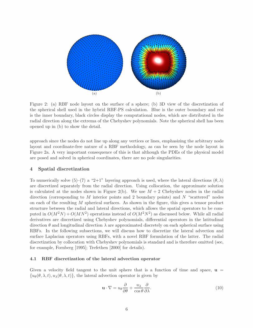
Figure 2: (a) RBF node layout on the surface of a sphere; (b) 3D view of the discretization ofthe spherical shell used in the hybrid RBF-PS calculation. Blue is the outer boundary and redis the inner boundary, black circles display the computational nodes, which are distributed in theradial direction along the extrema of the Chebyshev polynomials. Note the spherical shell has beenopened up in (b) to show the detail.

approach since the nodes do not line up along any vertices or lines, emphasizing the arbitrary nodelayout and coordinate-free nature of a RBF methodology, as can be seen by the node layout inFigure 2a. A very important consequence of this is that although the PDEs of the physical modelare posed and solved in spherical coordinates, there are no pole singularities.

4 Spatial discretization

To numerically solve (5)–(7) a “2+1” layering approach is used, where the lateral directions (θ, λ)are discretized separately from the radial direction. Using collocation, the approximate solutionis calculated at the nodes shown in Figure 2(b). We use M + 2 Chebyshev nodes in the radialdirection (corresponding to M interior points and 2 boundary points) and N “scattered” nodeson each of the resulting M spherical surfaces. As shown in the figure, this gives a tensor productstructure between the radial and lateral directions, which allows the spatial operators to be com-puted in O(M2N)+ O(MN2) operations instead of O(M2N2) as discussed below. While all radialderivatives are discretized using Chebyshev polynomials, differential operators in the latitudinaldirection θ and longitudinal direction λ are approximated discretely on each spherical surface usingRBFs. In the following subsections, we will discuss how to discretize the lateral advection andsurface Laplacian operators using RBFs, with a novel RBF formulation of the latter. The radialdiscretization by collocation with Chebyshev polynomials is standard and is therefore omitted (see,for example, Fornberg [1995]; Trefethen [2000] for details).

4.1 RBF discretization of the lateral advection operator

Given a velocity field tangent to the unit sphere that is a function of time and space, u =uθ(θ, λ, t), uλ(θ, λ, t), the lateral advection operator is given by

u · ∇ = uθ

∂

∂θ+

uλ

cos θ

∂

∂λ. (10)

6

which is singular at θ = ±π

2, the north and south poles, unless

∂

∂λalso vanishes there. We will

next see that this is exactly what happens when the operator is applied to an RBF.

Setting ε = 1 (for simplicity of notation), let φj(d) = φ(√

2(1 − cos θ cos θj cos(λ − λj) − sin θ sin θj))be an RBF centered at the node (θj, λj). Using the chain rule, the partial derivatives of the RBFφj(d) with respect to λ and θ are given by

∂

∂λφj(d) =

∂d

∂λ

∂φ

∂d= cos θ cos θj sin(λ − λj)

(1

d

∂φj

∂d

), (11)

∂

∂θφj(d) =

∂d

∂θ

∂φ

∂d= (sin θ cos θj cos(λ − λj) − cos θ sin θj)

(1

d

∂φj

∂d

). (12)

Inserting (11) and (12) into (10), we have

u · ∇ = uθ(cos θj sin θ cos(λ − λj) − sin θj cos θ)

(1

d

∂φj

∂d

)+ uλ cos θj sin(λ − λj)

(1

d

∂φj

∂d

). (13)

Given that the velocities are smooth, notice that nowhere on the sphere is (13) singular.

Now, we have all the components that are necessary to build the action of the advection operatoron an RBF representation of the temperature field. We first represent T (λ, θ) as an RBF expansiongiven by

T (θ, λ) =

N∑

j=1

cjφj(d(θ, λ)). (14)

where cj are the unknown expansion coefficients. We then apply the exact differential operatoru ·∇ to (14) and evaluate it at the node locations, (λi, θi)

Ni=1, where T (λ, θ) is known. Note that

because uλ and uθ are time-dependent we will need to create two separate differentiation matrices,

one to represent1

cos θ

∂

∂λφj(d) and another to represent

∂

∂θφj(d), otherwise (13) could be written

as a single differentiation matrix. Since they are created in the same way, we will only demonstratehow to formulate Dλ, the differentiation matrix for the longitudinal direction:

(a) Take1

cos θ

∂

∂λof (14):

1

cos θ

∂T (λ, θ)

∂λ=

N∑

j=1

cj

1

cos θ

∂φj(d)

∂λ=

N∑

j=1

cj cos θj sin(λ − λj)

(1

d

∂φj

∂d

).

(b) Evaluate (a) at the node locations:

N∑

j=1

cj

(cos θj sin(λi − λj)

1

d

∂φj

∂d

)∣∣∣∣(λ,θ)=(λi,θi)N

i=1︸ ︷︷ ︸Components of matrix Bλ

= Bλc,

where c contains the N unknown discrete expansion coefficients. If we evaluate the RBFs in (14)

7

at the node locations (λi, θi)Ni=1 then we have the collocation problem

φ(‖x1 − x1‖) φ(‖x1 − x2‖) · · · φ(‖x1 − xN‖)φ(‖x2 − x1‖) φ(‖x2 − x2‖) · · · φ(‖x2 − xN‖)

......

. . ....

φ(‖xN − x1‖) φ(‖xN − x2‖) · · · φ(‖xN − xN‖)

︸ ︷︷ ︸A

c1

c2...

cN

︸ ︷︷ ︸c

=

T1

T2...

TN

︸ ︷︷ ︸T

, (15)

where A is the RBF interpolation matrix for the node set. Thus, c = A−1T and substitutingthis into (b) above gives DλT = Bλ(A−1T ), in other words Dλ = BλA−1. Put verbally, thedifferentiation matrices are obtained by applying the exact differential operator to the interpolantand then evaluating it at the data locations. Although the computation of Dλ and Dθ requiresO(N3) operations, it is a pre-processing step that needs to be done only once.

4.2 A novel RBF surface Laplacian formulation

Since RBFs do not require the nodes on a spherical surface to have any directionality and sinceRBFs are not defined in terms of any surface based coordinate system (as discussed in Section 3),then for simplicity let us center an RBF at the north pole xnp = (0, 0, 1) or (θ, λ) = (π/2, 0). Thedistance from this point to any point on the sphere is then given by

d(x) = ‖x − xnp‖ =√

x2 + y2 + (z − 1)2 =√

2(1 − sin(θ)). (16)

Now, the surface Laplacian in spherical coordinates in given by

∆s =∂2

∂θ2− tan θ

∂

∂θ+

1

cos2 θ

∂2

∂λ2. (17)

However, for a radial function centered at the north pole there will be no λ dependence. So, (17)reduces to

∆s =∂2

∂θ2− tan θ

∂

∂θ. (18)

Applying (18) to an RBF φ(d) gives

∆sφ(d) =∂2d

∂θ2

∂φ

∂d+

(∂d

∂θ

)2 ∂2φ

∂d2− tan θ

∂d

∂θ

∂φ

∂d. (19)

With the use of (16) and after some algebra, (19) reduces to

∆sφ(d) =1

4

[(4 − d2)

∂2φ

∂d2+

4 − 3d2

d

∂φ

∂d

]. (20)

Although we derived this formula by centering the RBF at the north pole, any node could haveserved as the north pole since an RBF is invariant to coordinate rotations. The beauty of (20) isthat it expresses the action of the surface Laplacian on an RBF simply in terms of the distancesbetween nodes without the coordinate system ever coming into play. The RBF surface Laplaciandifferentiation matrix is then defined as Ls = BsA

−1, where Bs is now a matrix, evaluating (20) atd =

√2(1 − cos θi cos θj cos(λi − λj) − sin θi sin θj)), 1 ≤ i, j ≤ N , j indexing the RBF centers and

i the node locations.

8

Variable PDE Boundary Conditions at r = Ri, Ro Time-dependent

Ωh ∆Ωh = Ra r T Ωh |Ri,Ro= 0 Yes

Φh ∆Φh = Ωh Φh |Ri,Ro= 0 Yes

ΩRi

j ∆ΩRi

j = 0 ΩRi

j |Ro= 0, ΩRi

j |Ri=

1 if (θ, λ) = (θj, λj),

0 otherwise,No

ΦRi

j ∆ΦRi

j = ΩRi

j ΦRi

j |Ri,Ro= 0 No

ΩRo

j ∆ΩRo

j = 0 ΩRo

j |Ri= 0, ΩRo

j |Ro=

1 if (θ, λ) = (θj, λj),

0 otherwiseNo

ΦRo

j ∆ΦRo

j = ΩRo

j ΦRo

j |Ri,Ro= 0 No

ΩRi

bd,j, ΩRo

bd,j see (22)-(23) not applicable Yes

Table 2: The variables composing the influence matrix method with the PDEs and boundaryconditions they solve, and if they are time-dependent (i.e. need to be solved at every time step).

5 Momentum equations solver and influence matrix method

We cannot directly solve (5) and (6) since we have 4 boundary conditions on Φ, given by (8),and none on Ω. We therefore use the influence matrix method [Peyret, 2002] to find the unknownboundary values on Ω such that all 4 boundary conditions on Φ are satisfied. Since (5) and (6) arelinear, the solution to each Poisson equation can be represented as a superposition of two solutions;the first, Ωh and Φh, satisfies the right hand side of the equations with homogeneous Dirichletboundary conditions; the second, Ωj and Φj , couples the unknown boundary values (abbreviated

bd), ΩRi

bd,j and ΩRo

bd,j , with ΦRi

j and ΦRo

j at each RBF collocation node, θj , λjNj=1, on the inner (Ri)

and outer (Ro) boundary spherical surfaces, respectively. In Table 2, the variables are defined interms of the Poisson equations they solve with the overall solution written as

Ω = Ωh +

N∑

j=1

[ΩRi

bd,jΩRi

j + ΩRo

bd,jΩRo

j

]and Φ = Φh +

N∑

j=1

[ΩRi

bd,jΦRi

j + ΩRi

bd,jΦRo

j

]. (21)

The method is reminiscent of a Green’s function type approach, but instead of expanding thesource term of the PDEs in Dirac delta functions, we expand the unknown boundary conditions inthis basis, solve Laplace’s equation (as the right hand side is taken care of by the solutions Ωh andΦh) and superpose the solutions as is done by the summations in (21). Thus, for each boundary,we are building a table of N particular solutions, ΩRi

j Nj=1 and ΩRo

j Nj=1, whose boundary value

is 1 at the jth boundary node and 0 at all others. These PDEs are solved N times, correspondingto the number of boundary nodes we have on each boundary surface. It is important to note thatsolving for ΩRi

j and ΩRo

j is a pre-processing step, since the equation is temperature-independent

and thus time-independent. Also, once we solve for ΦRi

j and ΦRo

j , ΩRi

j and ΩRo

j can be deleted asthey are no longer needed for any computations. As discussed in Appendix A, the approximatesolutions to the PDEs listed in Table 2 are computed in spectral space via a matrix diagonalization(or eigenvector decomposition) technique which requires O(MN2) + O(M2N) operations per PDEand O(M2) + O(N2) storage. This is significant savings over a direct solve of the equations, whichwould require O(M2N2) operations and O(M2N2) storage.

9

Once Φh has been computed, the unknown coefficients ΩRi

bd,j and ΩRo

bd,j are determined by requiring

the linear combination of Φh, ΦRi

j , and ΦRo

j in (21) satisfy the boundary conditions (8). Sinceeach of these variables satisfy the homogeneous Dirichlet boundary conditions by construction, theunknown coefficients are determined by the second Neumann-type boundary condition. Insertingthe expression for Φ given in (21) into this boundary condition leads to the following set of linearequations which need to be enforced at each boundary node j = 1, . . . , N :

∂2

∂r2ΦRi

j

∣∣∣∣r=Ri

ΩRi

bd,j +∂2

∂r2ΦRo

j

∣∣∣∣r=Ri

ΩRo

bd,j = −∂2

∂r2Φh

∣∣∣∣r=Ri

, (22)

∂2

∂r2ΦRi

j

∣∣∣∣r=Ro

ΩRi

bd,j +∂2

∂r2ΦRo

j

∣∣∣∣r=Ro

ΩRo

bd,j = −∂2

∂r2Φh

∣∣∣∣r=Ro

. (23)

The coefficient matrix that arises from this 2N × 2N linear systems is called the influence matrixand can be pre-calculated, LU decomposed and stored as it is time-independent. However, thesolution to the linear system must be computed every time-step as Φh is time-dependent. OnceΩRi

bd,j and ΩRo

bd,j are found, Φ can be determined from the second equation in (21) and then thevelocity field can be calculated according to (9).

While the presentation above is the most straightforward way to describe the influence matrixtechnique for solving equations (5) and (6) subject to the boundary conditions (8), it is not themost computationally efficient given how the solutions to Ωh and Φh are computed in the overallalgorithm. In Appendix A, we discuss how the computation can be done in the spectral space ofthe discrete operators to reduce the computational cost. This description is the one used in thecode.

6 Time discretization

The Chebyshev discretization of the radial component of the diffusion operator has a Courant-Fredirchs-Lewey (CFL) condition on the time-step that is proportional to O(1/M4), which makesan explicit scheme implausible. As a result, we implement a semi-implicit time stepping schemewhich treats this component implicitly and the remaining terms of the energy equation explicitly.We note that implicitly time-stepping the entire diffusion term, that is also the RBF discretizationof the ∆s operator, would make no difference in terms of the overall CFL condition on the energyequation. This is because the CFL condition on this operator results in a time step restriction thatscales like O(1/N), with N = O(1000) typically, and the time step restriction due to the Chebyshevdiscretization on the radial components of the nonlinear advection term scales as O(1/M2), withM = O(10) typically.

We separate the terms in the energy equation (7) as follows:

∂T

∂t= −

(ur

∂T

∂r+ uθ

1

r

∂T

∂θ+ uλ

1

r sin θ

∂T

∂λ

)+

1

r2∆sT

︸ ︷︷ ︸f(T,t)

+1

r2

∂

∂r

(r2 ∂T

∂r

)

︸ ︷︷ ︸g(T,t)

. (24)

Using a third order Adams-Bashforth (AB3) method combined with a Crank-Nicolson (CN) method,(24) can be discretized by

T k+1 = T k +∆t

12(23F k − 16F k−1 + 5F k−2)

︸ ︷︷ ︸AB3

+∆t

2(Gk+1 + Gk)

︸ ︷︷ ︸CN

, (25)

10

Matrix Operator Discretization Dimension

Dλ

1

cos θ

∂

∂λRBF N × N

Dθ

∂

∂θRBF N × N

Ls ∆s RBF N × N

Dr

∂

∂rChebyshev M × M

Lr∂

∂r

(r2 ∂

∂r

)Chebyshev M × M

Table 3: Notation for the various differentiation matrices used in the time-differencing scheme.

where all the terms are matrices of size N × M , corresponding to the values in the interior of thespherical shell, and F k and Gk are the respective approximations to f(T, t) and g(T, t) at the kth

time step and are explicitly given by

F k = −(ukr (T kDr) + uk

θ (DθTkR−1) + uk

λ (DλT kR−1)) + LsTkR−2 + Bf

Gk = T kLrR−2 + Bg.

(26)

where denotes element-wise matrix multiplication, and Bf and Bg contain the appropriate termsfrom the boundary conditions on T . The abbreviations for the differentiation matrices are givenin Table 3. The matrices uk

r , ukθ , uk

λ are the approximations to the respective components of thevelocity at the kth time-step, while the diagonal matrix R contains the M interior Chebyshev nodes,defined by

Rj,j =1

2(Ri + Ro) +

1

2(Ro − Ri) cos

(j

M + 1π

), j = 1, . . . ,M. (27)

Equation (25) can be re-written as

T k+1 =

[T k +

∆t

12(23F k − 16F k−1 + 5F k−2) +

∆t

2Gk

](I −

∆t

2LrR

−2

)−1

(28)

As a pre-processing step (I − ∆t2 LrR

−2) is LU decomposed and stored. The computational costof computing (28) is then O(M2N). However, since N is typically two orders of magnitude largerthan M , the total cost per time step will be dominated by the solving the momentum equations(see Appendix A), calculating the velocity, and computing the values of F k and Gk, all of whichrequire O(MN2) operations. Exact details on each step of the algorithm are given in Appendix B.

7 Validation on the RBF-PS Method

In this section, we first consider three benchmark studies for 3D spherical shell models of mantleconvection with constant viscosity and report the first results in the literature from a purely spectralmethod run at Ra = 106. Although there are many numerical methods in the literature for mantleconvection in spherical geometry [Bercovici et al., 1989; Zhang and Christensen, 1993; Ratcliff et al.,1996; Richards et al., 2002; Hernlund and Tackley, 2003; Yoshida and Kageyama, 2004; Harder andHansen, 2005; Stemmer et al., 2006; Choblet et al., 2007; Kameyama et al., 2008; Zhong et al.,2000, 2008], the obstacle we encountered is that there is not a set of standardized test cases forcomparison with regard to Ra number and the viscosity profile. However, there are a number of

11

(a) (b)

Figure 3: θ − λ dependence of the initial condition for the (a) Tetrahedral and (b) Cubic mantleconvection test cases.

published results for Ra=7000 with constant viscosity and we compare our method with these.Above this Ra, there does not seem to be any consistency in the specifications of the physicalmodel for testing the numerical methods published in the literature. Thus, for higher Ra, we havedecided to use Ra = 105 results from the model for mantle convection, CitcomS, recently reportedin Zhong et al. [2008] as a benchmark comparison. The only other study in the literature thatgives isoviscous results for this Ra number is by Ratcliff et al. [1996], which is also included in ourcomparison.

7.1 Ra = 7000

The two most common benchmarks for computational models of mantle convection in a sphericalshell are the steady-state tetrahedral and cubic test cases. For both of these benchmarks the fluidis treated as isoviscous and Ra is set to 7000. The initial condition for the temperature is specifiedas

T (r, θ, λ) =Ri(r − Ro)

r(Ri − Ro)+ 0.01Y 2

3 (θ, λ) sin

(π

r − Ri

Ro − Ri

)(29)

for the Tetrahedral test case and

T (r, θ, λ) =Ri(r − Ro)

r(Ri − Ro)+ 0.01

[Y 0

4 (θ, λ) +5

7Y 4

4 (θ, λ)

]sin

(π

r − Ri

Ro − Ri

)(30)

for the Cubic test case, where Y m` denotes the normalized spherical harmonic of degree ` and order

m. The first term in each of the initial conditions represents a purely conductive temperatureprofile, while the second terms are perturbations to this profile and determine the final steady-statesolution. The θ − λ temperature dependence of (29) and (30) on a spherical shell surface can beseen in Figures 3(a) and 3(b), respectively.

For this test case, two RBF-PS simulations are reported: 1) a higher resolution case, N = 1600nodes were used on each spherical surface (i.e. in the lateral directions) and 23 total Chebyshevnodes were used in the radial direction (i.e. M = 21 total interior nodes), giving a total of 36,800nodes and 2) a lower resolution case of N = 900 and 19 nodes radially (17 interior nodes), giving atotal of 17,100 nodes. A time-step of 10−4 was used or 10,000 time steps were taken to reach steady-state at the non-dimensionalized time of t = 1, corresponding to roughly 58 times the age of theEarth. Figures 4(a) and 4(b) display the final RBF-PS steady-state solutions for the Tetrahedral

12

(a) (b)

Figure 4: Steady-state isosurfaces of the residual temperature, δT , at t = 1 for the isoviscous (a)Tetrahedral and (b) Cubic mantle convection test cases at Ra = 7000 computed with the RBF-PSmodel. Yellow corresponds to δT = 0.15 and denotes upwelling relative to the average temperatureat each radial level, while blue corresponds to δT = −0.15 and denotes downwelling. The red solidsphere shows the inner boundary of the 3D shell corresponding to the core.

and Cubic test cases, respectively, in terms of the residual temperature δT = T (r, θ, λ) − 〈T (r)〉,where 〈 〉 denotes averaging over a spherical surface. Since no analytical solutions exist, validationis done via comparison to other published results in the literature with respect to scalar globalquantities, such as Nusselt number at the inner and outer boundaries (Nui and Nuo), and theaveraged root mean square velocity and temperature over the volume. Table 4 contains such acomparison for the RBF-PS method with respect to popular methods used in the mantle convectionliterature. The following observations can be can be made:

1. The only method that is spectral in at least one direction is the spherical harmonic-finitedifference method of Harder [1998]. In Stemmer et al. [2006], Harder’s method was used withRomberg extrapolation to obtain the results to at least four digits of accuracy. With regardto almost all quantities for both test cases, the results of the RBF-PS method match exactlywith Harder’s extrapolated results.

2. The number of nodes (degrees of freedom) needed to accomplish the results in point 1 is anorder of magnitude lower than what was used with the CitcomS model reported by Zhonget al. [2008], approximately one and a half orders of magnitude lower than either the finitevolume method by Stemmer et al. [2006] or the method by Harder [1998] and three orders ofmagnitude less than the Yin-Yang, multigrid method by Kameyama et al. [2008]. It should benoted, however, that with exception to the Stemmer et al. [2006] and Harder [1998] results,a detailed convergence study was not performed for these methods to determine the minimaldegrees of freedom needed to acheive their reported results.

3. For the scheme to conserve energy Nui = Nuo, notice this is the case for both tests even withsuch a low number of nodes. This results from the spectral accuracy of the RBF-PS method,which by its shear high-order convergence, will inherently dissipate physical quantities less.

4. Even though we are using Chebyshev polynomials in the radial direction and an explicit time-stepping scheme for the advection term in the temperature equation, we still can take thesame number of total time steps as Zhong et al. [2008] (i.e. 10,000).

13

5. Even if we decrease the number of nodes by over 50%, there is only very minor changes inthe results. From our calculations, it seems that at least 17 interior nodes (19 total nodes)are needed in the radial direction to resolve the flow at Ra = 7000. Although not reported,we found that in the lateral direction the number of RBF nodes could be reduced by another20% and the values reported changed only slightly (in the third decimal place).

7.2 Ra = 105

For the isoviscous Ra = 105 case, there are only two published studies for comparison, the CitcomSstudy of Zhong et al. [2008] and Ratcliff et al. [1996]. Both use the cubic test case initial conditiongiven by (30) and the model is integrated to approximately t = 0.3. Since Ra = 105 is a moreconvective regime, resulting in thinner plumes as seen in Figures 5(a) and 5(b), larger resolution isneeded. Thus, we use 43 Chebyshev nodes (41 interior nodes) in the radial direction and 4096 nodeson each spherical surface. Since the time step is purely restricted by the Chebyshev discretization,the increase in Chebyshev nodes results in a more severe CFL criterion that causes a necessarydecrease in the time step. The time step for this case is 6 · 10−5 for stability or 50,000 time stepsto reach t = 0.3 as opposed to the 35,000 time steps used by Zhong et al. [2008].

Comparative results are given in Table 5. The following 5 points are notable:

1. The difference between Nuo and Nui is 0.14%, showing that we are close to absolute conser-vation of energy.

2. The results of the RBF-PS method are much closer to that of Zhong et al. [2008] than tothose of Ratcliff et al. [1996]. We attribute this difference, most likely, to the under-resolutionof the runs of the latter model.

3. The RBF-PS uses approximately an order of magnitude less degrees of freedom than thestudy by Zhong et al. [2008].

4. Once steady state has been reached, differences between our results and those of Zhong et al.[2008] are within: 0.4% for Nuo and Nui, 0.2% for 〈Vrms〉, and 0.9% for 〈T 〉.

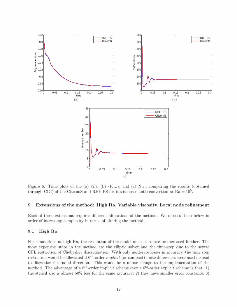
5. Even during the startup of the model, the curves for Nuo, 〈Vrms〉, and 〈T 〉 as a function oftime, are almost indistinguishable from the results of Zhong et al. [2008], as seen in Figures6(a)–(c).

7.3 Ra = 106

Since no results from a purely spectral method have ever been reported in 3D spherical geometryat Ra = 106, we have decided to include this result. The common practice at this and larger Ra isto start the simulation with an initial condition taken from a simulation run at a lower Ra. Theprimary reason for this is to avoid the extremely high velocity values that occur at higher Ra duringthe initial redistribution of the temperature from a conductive profile to a convective profile, whichseverely restricts the time-steps that can be taken. The initial condition used at Ra = 106 wastaken from a simulation which was started at Ra = 105 with an initial condition consisting of twoterms, a purely conductive temperature profile plus a small perturbation in the lateral directionthat randomly combined all spherical harmonics up to degree 10. This latter term was multiplied

14

Model Type Nodes r × (θ × λ) Nuo Nui 〈Vrms〉 〈T 〉

Cubic test case, Ra = 7000

Zhong [2008] FE 393216 32 × (12 × 32 × 32) 3.6254 3.6016 31.09 0.2176

Yoshida [2004] FD 2122416 102 × (102 × 204) 3.5554 — 30.5197 —

Kameyama [2008] FD 12582912 128 × (2 × 128 × 384) 3.6083 — 31.0741 0.21639

Ratcliff [1996] FV 200000 40 × (50 × 100) 3.5806 — 30.87 —

Stemmer [2006] FV 663552 48 × (6 × 48 × 48) 3.5983 3.5984 31.0226 0.21594

Stemmer [2006] FV Extrap. Extrap. 3.6090 — 31.0709 0.21583

Harder [1998; 2006] SP-FD 552960 120 × (48 × 96) 3.6086 — 31.0765 0.21582

Harder [1998; 2006] SP-FD Extrap. Extrap. 3.6096 — 31.0821 0.21578

RBF-PS SP 36800 23 × (1600) 3.6096 3.6096 31.0820 0.21577

RBF-PS SP 17100 19 × (900) 3.6098 3.6098 31.0834 0.21579

Tetrahedral test case, Ra = 7000

Zhong [2008] FE 393216 32 × (12 × 32 × 32) 3.5126 3.4919 32.66 0.2171

Yoshida [2004] FD 2122416 102 × (102 × 204) 3.4430 — 32.0481 —

Kameyama [2008] FD 12582912 128 × (2 × 128 × 384) 3.4945 — 32.6308 0.21597

Ratcliff [1996] FV 200000 40 × (50 × 100) 3.4423 — 32.19 —

Stemmer [2006] FV 663552 48 × (6 × 48 × 48) 3.4864 3.4864 32.5894 0.21564

Stemmer [2006] FV Extrap. Extrap. 3.4949 — 32.6234 0.21560

Harder [1998; 2006] SP-FD 552960 120 × (48 × 96) 3.4955 — 32.6375 0.21561

Harder [1998; 2006] SP-FD Extrap. Extrap. 3.4962 — 32.6424 0.21556

RBF-PS SP 36800 23 × (1600) 3.4962 3.4962 32.6424 0.21556

RBF-PS SP 17100 19 × (900) 3.4964 3.4963 32.6433 0.21557

Table 4: Comparison between computational methods for the isoviscous Tetrahedral and Cubicmantle convection test cases with Ra = 7000. Nuo and Nui denote the respective Nusselt number atthe outer and inner spherical surfaces, 〈Vrms〉 the volume-averaged RMS-velocity over the 3D shell,and 〈T 〉 the mean temperature of the 3D shell. Extrap. indicates that the results were obtainedusing Romberg extrapolation. Solid lines indicate numbers were not reported. Abbreviations: FE= finite element, FD = finite difference, FV = finite volume, SP-FD = hybrid spectral and finitedifference, and SP = purely spectral. For the RBF-PS method, the standard deviation of all thequantities from the last 1000 time-steps was less than 5 · 10−5, which is a standard measure forindicating the model has reached numerical steady-state.

by the same sine term in the radial direction as used in the previous cases. For the discretization,we used 81 Chebyshev nodes in the radial direction and 6561 nodes on each spherical surface, fora total of 531,441 nodes. The Ra = 105 simulation was run until the large spike in the radialvelocity subsided, the Ra was then increased to 5 · 105 and the simulation was restarted with theRa = 105 solution as the initial condition. This process was repeated once more and the Ra was

15

(a) (b)

Figure 5: (a) Steady-state isosurface temperature T = 0.5 at time t = 0.3. (b) Steady-stateisosurface of the residual temperature, δT = T (r, λ, θ) − 〈T (r)〉, at t = 0.3 for the isoviscous cubicmantle convection test case at Ra = 105 computed with the RBF-PS model. The same color schemeas Figure 4 has been applied.

Model Type Nodes r × (θ × λ) Nuo Nui 〈Vrms〉 〈T 〉

Zhong [2008] FE 1,327,104 48 × (12 × 48 × 48) 7.8495(0.0054)

7.7701(0.001)

154.8(0.04)

0.1728(0.0002)

Ratcliff [1996] FV 200,000 40 × (50 × 100) 7.5669 — 157.5 —

RBF-PS SP 176,128 43 × (4096) 7.8120 7.8005 154.490 0.17123

Table 5: Comparison between computational methods for the isoviscous Cubic mantle convectiontest case with Ra = 105. Numbers in parenthesis for Zhong et al. [2008] represent standarddeviations. The standard deviation of the results from the last 1000 time-steps for the RBF-PSmodel were all less than 5 · 10−5.

then increased to 106 and the time was reset to 0. The Ra = 106 simulation results from t = 0 tot = 0.08 (approximately 4 and half times the age of the Earth), are displayed in Figure 7. Part(a) of this figure displays the isosurfaces of the residual temperature at t = 0.08 and clearly showsthe mantle in a purely convective regime. Figures 7(b)–(d) show the time traces of 〈T 〉, 〈Vrms〉,and Nuo and Nui, respectively. Since this is a purely convective regime the choice of ending timeis somewhat arbitrary. We chose to stop the simulation at t = 0.08 since by this time the averagetemperature had decreased to an acceptable level from its initial starting value and the influenceof the initial condition had diminished.

8 Timing results

In this short section, a table of runtime results are presented in order to give the reader a feel forhow long it takes to run the code. All test cases were conducted on a workstation with one Inteli7 940 2.93 GHz processor, which is a quad core processor. The code was written in Matlab andrun under version 2009b with BLAS multi-threading enabled. 8 GB of memory was also availablefor the calculations, although only a fraction of this was actually used. The results under ‘Totalruntime’ in Table 6 include the pre-processing steps in the Appendix B, such as setting up thedifferentiation matrices and diagonalizing them.

16

0 0.05 0.1 0.15 0.2 0.25 0.30.16

0.18

0.2

0.22

0.24

0.26

0.28

0.3

0.32A

vg. t

empe

ratu

re

time

RBF−PSCitcomS

(a)

0 0.05 0.1 0.15 0.2 0.25 0.30

100

200

300

400

500

600

700

800

RM

S v

eloc

ity

time

RBF−PSCitcomS

(b)

0 0.05 0.1 0.15 0.2 0.25 0.30

5

10

15

20

25

30

35

Nus

selt

num

ber

time

RBF−PSCitcomS

(c)

Figure 6: Time plots of the (a) 〈T 〉, (b) 〈Vrms〉, and (c) Nuo, comparing the results (obtainedthrough CIG) of the CitcomS and RBF-PS for isoviscous mantle convection at Ra = 105.

9 Extensions of the method: High Ra, Variable viscosity, Local node refinement

Each of these extensions requires different alterations of the method. We discuss them below inorder of increasing complexity in terms of altering the method.

9.1 High Ra

For simulations at high Ra, the resolution of the model must of course be increased further. Themost expensive steps in the method are the elliptic solver and the time-step due to the severeCFL restriction of Chebyshev discretization. With only moderate losses in accuracy, the time steprestriction would be alleviated if 6th-order implicit (or compact) finite differences were used insteadto discretize the radial direction. This would be a minor change to the implementation of themethod. The advantage of a 6th-order implicit scheme over a 6th-order explicit scheme is that: 1)the stencil size is almost 50% less for the same accuracy; 2) they have smaller error constants; 3)

17

(a)

0 0.01 0.02 0.03 0.04 0.05 0.06 0.07 0.080.195

0.2

0.205

0.21

0.215

0.22

0.225

0.23

0.235

0.24

time

Avg

. tem

pera

ture

(b)

0 0.01 0.02 0.03 0.04 0.05 0.06 0.07 0.08500

550

600

650

700

750

800

850

time

RM

S v

eloc

ity

(c)

0 0.01 0.02 0.03 0.04 0.05 0.06 0.07 0.084

6

8

10

12

14

16

18

20

22

24

time

Nu

Nu

I

NuO

(d)

Figure 7: Results for Ra = 106 test case: (a) Residual temperature, δT , at t = 0.08, where yellowcorresponds to δT = 0.1, blue corresponds to δT = −0.1, and the red solid sphere shows the innerboundary of the 3D shell corresponding to the core; (b) Average temperature, 〈T 〉, vs. time; (c)Average RMS velocity, 〈Vrms〉, vs. time; (d) Inner and outer Nusselt numbers, Nui and Nuo, vs.time.

Test Total number Runtime per Total Total Time

Case of nodes time-step runtime steps

Ra = 7000 36,800 0.0516 sec. 8 min. 16 sec. 10,000 (to t=1)

Ra = 100,000 176,128 0.44 sec. 6 hours 27 min. 50,000 (to t=0.3)

Table 6: Runtime results for the RBF-PS method for the Ra=7000 and Ra=100,000 cases on asingle 2.93GHz Intel i7 940 quad core processor.

18

information only needs to be extrapolated to one point outside the boundary; 4) most importantly,they have spectral-like resolution in the sense that they resolve higher wavenumbers [Lele, 1992].To date, the authors are not aware of a study that has employed such a scheme. With regard to theelliptic solver, global RBFs do not scale well as high Ra convection is reached (i.e. Ra ∼ O(109)).However, RBF-based finite difference schemes (see Section 9.3 below), already show exceptionallypromising results on spherical surfaces, in terms computational scaling and accuracy [Fornberg andLehto, 2010; Flyer et al., 2010].

9.2 Variable viscosity

To handle variable viscosity (depth and/or horizontal dependent), the PDEs in their primitivevariables, i.e. (1) and (2), would need to be discretized. The main difficulty here is not in thediscretization of the variable coefficients terms that appear in (2), which can be handled straight-forwardly by the method, but from solving the resulting coupled equations to ensure that the flowremains incompressible. This system will be of saddle point type for which many potential methodsare available (see, for example, the review by Benzi et al. [2005]). The most promising approachfor the RBF-PS system, currently being explored by authos, would use a block factorization ofthe discretized momentum and continuity equations, giving an upper block triangular system andresulting in a Schur complement problem. To avoid the excessive computational cost in solving thissystem directly at every time-step, we would instead employ a pre-conditioned Krylov subspacemethod (see Section 10 of [Benzi et al., 2005] for a discussion). A good choice for the preconditionermight be to use a coarse solution to the isoviscous problem, as presented by the method in Section5, since the velocities should be sufficiently smooth given that they are solutions to Poisson-typePDEs.

9.3 Local refinement

Local refinement will take the greatest alteration to the code. Once variables are separated, inthis case (θ, λ) from r, the result is a tensor-like grid and local refinement becomes difficult. ForRBFs, refinement is simple in the sense that the nodes can be easily clustered [Flyer and Lehto,2009]. Thus, the next developmental step, which is currently in progress, is to use 3D RBF-based finite difference stencils [Wright and Fornberg, 2006] for discretizing the equations. Here,all differentiation matrices are based on local high-order finite difference-type stencils that aregenerated by means of RBFs from nodes scattered in 3D space, which results in exceptionallysparse matrices to solve.

10 Summary

This paper develops the first spectral RBF method for 3D spherical geometries in the math/scienceliterature. Applications of this new hybrid purely spectral methodology are given to the problemof thermal convection in the Earth’s mantle, which is modeled by a Boussinesq fluid at infinitePrandtl number. To see whether this numerical technique warrants further investigation, the studylimits itself to an isoviscous mantle. Two Ra number regimes are tested, the classical case in theliterature of Ra=7000 and the latest results from the CitcomS model [Zhong et al., 2008] at Ra=105.Also, a Ra = 106 simulation is run, as there are no results in the literature from a purely spectralmodel at this Ra. For the Ra=7000 case, the method perfectly conserved energy, matched theextrapolated results of the only other partially spectral method (reported in Stemmer et al. [2006])to four or 5 significant digits and used anywhere between 1 to 3 orders of magnitude less nodes

19

than other methods. For the Ra=105 case, the method almost perfectly conserved energy, andgave results that differed from CitcomS by 0.2% to 0.9% (depending on the scalar quantity beingmeasured) yet required approximately an order of magnitude less nodes. All calculations were runon a workstation using a single quad core processor with Ra=7000 case taking about 8 minutesand the Ra=105 case taking about 6.5 hours. Given this outcome, the methodology warrants moreextensive testing. It will be altered to accommodate the PDEs in primitive form so that variableviscosity and thermochemical convection can be considered in future test runs.

We conclude by noting that the spectral RBF method presented here may also be a potentiallypromising technique for simulating the geodynamo, which is well approximated by an isoviscous andBoussinesq fluid. For the geodynamo, the Prandtl number is finite and the (now time-dependent)momentum and energy equations are coupled to a time-dependent induction equation for the mag-netic field (see, for example, Glatzmaier and Roberts [1995]). For the hybrid RBF method, a naturalapproach would be to decompose the velocity and magnetic fields into toroidal and poloidal poten-tials as is commonly done in other models (see, for example, Christensen et al. [2001]; Glatzmaierand Roberts [1995]; Oishi et al. [2007]). This decomposition results in a coupled set of time-dependent parabolic equations and a set of time-independent elliptic equations. For the former, asimilar approach to the discretization for the energy equation discussed in Section 6 could be used,while the latter could be solved using the technique discussed in Appendix A.

Acknowledgments G. B. Wright was supported by NSF grants ATM-0801309 and DMS-0934581.N. Flyer was supported by NSF grants ATM-0620100 and DMS-0934317 from the National ScienceFoundation. Flyer’s work was in part carried out while she was a Visiting Fellow at OCCAM(Oxford Centre for Collaborative Applied Mathematics) under support provided by Award No.KUK-C1-013-04 to the University of Oxford, UK, by King Abdullah University of Science andTechnology (KAUST). D. A. Yuen was supported by NSF grant DMS-0934564.

A Solution of the momentum equations via matrix diagonalization

The two coupled Poisson equations representing the momentum equations, are solved throughmatrix diagonalization (i.e. spectral decomposition) of the RBF surface Laplacian and Chebyshevradial operators, respectively, and the influence matrix method briefly discussed in Section 5. Inthis appendix, we first show how the two coupled equations in rows 1 and 2 of Table 2 are solvedfor Ωh and Φh. We then describe the influence matrix method in the spectral space of the discreteoperators. We conclude with details on how the full solution for Φ is obtained.

If N is the number of nodes on a spherical surface and M is the number of interior Chebyshev nodesin the radial direction, then let Ωh,Φh ∈ R

N×M be the respective matrices for the unknown valuesof the two potentials at all the interior node points at time t. Also let T ∈ R

N×M be the the knownvalues of the temperature at time t. Using the notation from Table 3 for the RBF differentiationmatrix for the surface Laplacian and the Chebyshev differentiation matrix for the radial componentof the 3D Laplacian, the discrete form of the first two equations in Table 2 is written as

LsΩh + ΩhLr =RaT R, (31)

LsΦh + ΦhLr =Ωh R2, (32)

where R is the diagonal matrix given in (27). Now, letting Ls = VsΛsV−1s and Lr = VrΛrV

−1r be

the spectral decompositions of the operators Ls and Lr, respectively, (31) and (32) can be written,

20

after some manipulations as

Λs(V−1s ΩhVr) + (V −1

s ΩhVr)Λr =Ra (V −1s T RVr),

Λs(V−1s ΦhVr) + (V −1

s ΦhVr)Λr =(V −1s ΩhVr)(V

−1r R2Vr).

By defining Ωh = V −1s ΩhVr, Φh = V −1

s ΦhVr, T = V −1s T RVr, and R2 = V −1

r R2Vr, the aboveequations can be written as the diagonal system of equations

ΛsΩh + ΩhΛr =Ra T , (33)

ΛsΦh + ΦhΛr =ΩhR2. (34)

The solutions to these equations are given explicitly as

(Ωh)i,j = Ra(T )i,j

(Λs)i,i + (Λr)j,jand (Φh)i,j =

(ΩhR2)i,j(Λs)i,i + (Λr)j,j

, (35)

for i = 1, . . . , N, and j = 1, . . . ,M .

The operators Ls and Lr are time-independent so that their spectral decompositions can be com-puted as a preprocessing step. The solution to (33) and (34) thus requires O(MN) operationsper time-step. However, the total cost in computing Φh per time-step is dominated by the costof computing T and ΩhR2, which requires O(MN2) and O(M2N) operations, respectively. SinceN is typically two orders of magnitude greater than M , the former computation will dominateeverything.

We also apply the influence matrix technique in spectral space as it allows some reduction in thestorage and computational cost of computing the final value of Φ. The setup of this technique issimilar to that described in Section 5 in that we look for a superposition of solutions to the equations.However, by working in the spectral space of the lateral operator Ls, the lateral directions can bedecoupled so that the superposition consists only of three N × M linear systems instead of N :

Ω = Ωh + ΩRi

bdΩRi + Ω

Ro

bd ΩRo

and Φ = Φh + ΩRi

bdΦRi + Ω

Ro

bd ΦRo

, (36)

where bars indicate the variables are in the spectral space of the lateral operator Ls only, and

ΩRi

bd and ΩRo

bd are N × N diagonal matrices with the unknown values for enforcing the boundaryconditions. The values of Ωh and Φh, can be obtained by multiplying Ωh and Φh (computed from(33) and (34)) on the right by V −1

r . The remaining values are determined from the solution ofN independent two-point boundary value systems in the radial direction which correspond to thetransform of the two sets of coupled PDEs in rows 3–6 of Table 2 into the spectral space of Ls.The complete set of equations can be written in discrete form as

ΛsΩ

Ri + ΩRiLr = BRi ,

ΛsΦRi + Φ

RiLr = ΩRiR2,

and

ΛsΩ

Ro

+ ΩRo

Lr = BRo,

ΛsΦRo

+ ΦRo

Lr = ΩRo

R2,(37)

where BRi and BRo contain the modifications from the boundary conditions (ΩRi)j = 1 at r = Ri

and (ΩRo

)j = 1 at r = Ro (the remaining boundary conditions on the variables are homogeneous).The solutions to both of these systems can be computed by a transformation into the the spectralspace of Lr as done in (33) and (34) and then solving a diagonal system. The total operation for

the solution of ΦRi and Φ

Ro

can then be computed in O(M2N) operations. However, this can bedone as a preprocessing step as these values are time-independent.

21

To find the unknown values on the diagonals of ΩRi

bd and ΩRo

bd we apply the second set of boundaryconditions in (8) to the right hand side of the Φ equation in (36). The discrete set of equationsthat result are given by

(Φ

RiDRi

rr

)Ω

Ri

bd +(Φ

Ro

DRi

rr

)Ω

Ro

bd = − ΦhDRi

rr , (38)(Φ

RiDRo

rr

)Ω

Ri

bd +(Φ

Ro

DRo

rr

)Ω

Ro

bd = − ΦhDRo

rr , (39)

where DRi

rr ,DRo

rr ∈ RM×1 are the discrete Chebyshev second derivative operators in the radial

direction at the inner and outer boundaries, respectively. Equations (38) and (39) correspond to Ndecoupled 2 × 2 linear system for finding the unknowns. Thus, all these systems can be solved in

O(N) operations. Furthermore, since ΦRi and Φ

Ro

are time independent the values in parenthesison the left hand side of these equations can be computed as a preprocessing step. The values onthe right hand side are time-dependent and need to be computed every time step, which requiresO(MN) operations.

Once ΩRi

bd and ΩRo

bd are determined, Φ is computed according to (36) and then transformed back intophysical space by computing Φ = VsΦ. The computation of Φ requires O(MN) operations and thecomputation of Φ requires O(MN2) operations. Combining this cost with the cost of computingΦh from (33) and (34), we see the total computational cost per time-step for computing Φ will beO(MN2) operations.

B Overview of RBF-PS Algorithm

Set-up (Pre-processing):

1. Discretize∂

∂θ,

1

cos θ

∂

∂λ, and ∆s using collocation with N RBFs. This will result in 3 N ×N

matrices, Dθ, Dλ, and Ls (see Sections 4.1 and 4.2).

2. Discretize∂

∂r,

∂

∂r

(r2 ∂

∂r

),

∂2

∂r2

∣∣∣∣r=Ri

, and∂2

∂r2

∣∣∣∣r=Ro

using collocation with M +2 Chebyshev

polynomials. Since these are only applied on the interior of the shell, this will result in 2M ×M matrices Dr and Lr for the first two operators, and 2 M × 1 vectors for the last two.

3. Form the M × M diagonal matrices R (see (27)) and R2.

4. LU decompose the M × M matrix (I − ∆t/2LrR−2) for the AB3-CN time stepping method

(see Section 6), where I is the M × M identity matrix.

5. Momentum equations:

(a) Compute the spectral decomposition of Ls and Lr (see Appendix A). This results in thefollowing matrices: 1 full N × N (Vs), 1 diagonal N × N (Λs), 1 full M × M (Vr), and1 diagonal M × M (Λr).

(b) Compute the inverses of Vr and Vs.

(c) Compute the full M × M matrix R2 = V −1r R2Vr.

(d) Solve (37) for ΦRi and Φ

Ro

, which results in 2 N × M matrices.

22

(e) Compute the influence matrix entries ΦRiDRi

rr , ΦRiDRo

rr , ΦRo

DRi

rr , and ΦRo

DRo

rr from (38)and (38). This results in 4 vectors of length N .

Execution:

1. Momentum equations:

(a) With the temperature T k at the kth time step, calculate Φh (i.e Φh in the spectral spaceof both the operators Ls and Lr) according to (35).

(b) Calculate Φh = ΦhV −1r (i.e Φh in the spectral space of Ls only).

(c) Solve for the influence matrix system (37) for the unknowns ΩRi

bd and ΩRo

bd .

(d) Compute Φ by updating Φh with the influence matrix terms according to (36).

(e) Compute Φ = VsΦ to find the poloidal potential in physical space.

(f) Compute the velocity field (9), which can be written

u = (LsΦR−1

︸ ︷︷ ︸ur

,DθΦRDrR−1

︸ ︷︷ ︸uθ

,DλΦRDrR−1

︸ ︷︷ ︸uλ

).

2. Compute the Fk and Gk in (26) with the velocity field from the previous step and the tem-perature T k.

3. Solve (28) for the temperature at the next time-step, T k+1, and repeat step 1 with this newtemperature.

References

G.E. Backus. Potentials for tangent tensor fields on spheroids. Arch. Rational Mech. Anal., 22:210–252, 1966. ISSN 0003-9527.

J. R. Baumgardner. Three dimensional treatment of convection flow in the Earth’s mantle. J.

Statistical Physics, 39 (5/6):501–511, 1985.

M. Benzi, G.H. Golub, and J. Liesen. Numerical solution of saddle point problems Acta Numerica,doi: 10.1017/S0962492904000212, 1–137, 2005.

D. Bercovici, G. Schubert, G. A. Glatzmaier, and A. Zebib. Three-dimensional thermal-convectionin a spherical shell. J. Fluid Mech., 206:75–104, 1989.

M. D. Buhmann. Radial Basis Functions: Theory and Implementations. Cambridge UniversityPress, 2003

S. Chandrasekhar. Hydrodynamic and Hydromagnetic Stability. Dover, 1961.

G. Choblet, O. Cadek, F. Couturier, and C. Dumoulin. Oedipus: a new tool to study the dynamicsof planetary interiors. Geophys. J. Int., 170:9–30, 2007.

CIG (Computational Infrastructure for Geodynamics). http://www.geodynamics.org/cig/

workinggroups/mc/workarea/benchmark/3dconvention/.

23

U. R. Christensen, J. Aubert, P. Cardin, E. Dormy, S. Gibbons, G. A. Glatzmaier, E. Grote, Y.Honkura, C. Jones, M. Kono, M. Matsushima, A. Sakuraba, F.Takahashi, A. Tilgner, J. Wicht,and K. Zhang. A numerical dynamo benchmark. Phys. Earth Planet. Inter., 128:25–34, 2001.

T. A. Driscoll and A. Heryundono. Adaptive residual subsampling methods for radial basis functioninterpolation and collocation problems. Comput. Math. Appl., 53:927–939, 2007.

G. E. Fasshauer. Meshless Approximation Methods with MATLAB. Interdisciplinary MathematicalSciences - Vol. 6. World Scientific Publishers, Singapore, 2007.

G. E. Fasshauer and J. G. Zhang. On choosing “optimal” shape parameters for RBF approximation.Numerical Algorithms, 45:345–368, 2007.

N. Flyer and E. Lehto. Rotational transport on a sphere: Local node refinement with radial basisfunctions. J. Comp. Phys., doi: 10.1016/j.jcp.2009.11.016, 2009.

N. Flyer and G. B. Wright. Transport schemes on a sphere using radial basis functions. J. Comp.

Phys., 226:1059–1084, 2007.

N. Flyer and G. B. Wright. A radial basis function method for the shallow water equations on asphere. Proc. Roy. Soc. A, 465:1949–1976, 2009.

N. Flyer and E. Lehto and G. B. Wright and A. St-Cyr. A radial basis function generated finitedifference method for the unsteady shallow water equations on a sphere. In preparation, 2010.

B. Fornberg. A Practical Guide to Pseudospectral Methods. Cambridge Univ. Press, 1995.

B. Fornberg, T. A. Driscoll, G. Wright, and R. Charles. Observations on the behavior of radialbasis functions near boundaries. Comput. Math. Appl., 43:473–490, 2002.

B. Fornberg and N. Flyer. Accuracy of radial basis function interpolation and derivative approxi-mations on 1-D infinite grids Adv. Comput. Math., 23:5–20, 2005.

B. Fornberg, N. Flyer, and J. M. Russell. Comparisons between pseudospectral and radial basisfunction derivative approximations. IMA J. Num. Analy., 30(1):149–172, 2010.

B. Fornberg and E. Lehto A filter approach for stabilizing RBF-generated finite difference methodsfor convective PDEs in preparation, 2010.

B. Fornberg and C. Piret. On choosing a radial basis function and a shape parameter when solvinga convective PDE on a sphere. J. Comp. Phys., 227:2758–2780, 2008.

B. Fornberg, G. Wright, and E. Larsson. Some observations regarding interpolants in the limit offlat radial basis functions. Comput. Math. Appl., 47:37–55, 2004.

B. Fornberg and J. Zuev. The runge phenomenon and spatially variable shape parameters in RBFinterpolation. Comput. Math. Appl., 54:379–398, 2007.

G. A. Glatzmaier and P. H. Roberts. A three-dimensional self-consistent computer simulation of ageomagnetic field reversal. Nature, 377:203–209, (1995).

H. Harder. Phase transitions and the three-dimensional planform of thermal convection in themartian mantle. J. Geophys. Res., 103:16775–16797, 1998.

24

H. Harder and U. Hansen. A finite-volume solution method for thermal convection and dynamoproblems in spherical shells. Geophys. J. Int, 161:522–532, 2005.

D. P. Hardin and E. B. Saff. Discretizing manifolds via minimum energy points. Notices Amer.

Math. Soc., 51:1186–1194, 2004.

J.W. Hernlund and P.J. Tackley. Three-dimensional spherical shell convection at infinite prandtlnumber using the cubed sphere method. In K. Bathe, editor, Computational Fluid and Solid

Mechanics, page 931. Elsevier, 2003.

C. Huettig and K. Stemmer. The spiral grid: A new approach to discretize the sphere and its ap-plication to mantle convection. Geochem. Geophys. Geosys., 9(2):, doi: 10.1029/2007GC001581,2008.

A. Iske. Multiresolution Methods in Scattered Data Modelling. Springer-Verlag, Heidelberg, 2004.

M. C. Kameyama, A. Kageyama, and T. Sato. Multigrid-based simulation code for mantle convec-tion in spherical shell using Yin-Yang grid. Phys. Earth Planet. Interiors, 171:19–32, 2008.

S. K. Lele. Compact finite difference schemes with spectral-like resolution. J. Comput. Phys., 103:16–42, 1992.

Y. Oishi, A. Sakuraba, and Y. Hamano. Numerical method for geodynamo simulations based onFourier expansion in longitude and finite difference in meridional plane. Phys. Earth Planet.

Interiors, 164:208–229, 2007.

R. Peyret. Spectral Methods for Incompressible Viscous Flow. Springer-Verlag, New York, 2002.

J.T. Ratcliff, G. Schubert, and A. Zebib. Steady tetrahedral and cubic patterns of spherical shellconvection with temperature-dependent viscosity. J. Geophys. Res., 101:473–484, 1996.

M.A. Richards, W.S. Yang, J.R. Baumgardner, and H.P. Bunge. Role of a low viscosity zonein stabilizing plate techtonics: Implications for comparative terrestrial planetology. Geochem.

Geophys. Geosyst., 3(7):1040, 2002.

K. Stemmer, H. Harder, and U. Hansen. A new method to simulate convection with stronglytemperature-dependent and pressure-dependent viscosity in spherical shell. Physics of the Earth

and Planetary Inter., 157:223–249, 2006.

L. N. Trefethen. Spectral Methods in MATLAB. SIAM, Philadelphia, 2000.

J. Wertz, E. J. Kansa, and L. Ling. The role of multiquadric shape parameters in solving ellipticpartial differential equations. Comput. Math. Appl., 51:1335–1348, 2006.

G. B. Wright and B. Fornberg. Scattered node compact finite difference-type formulas generatedfrom radial basis functions. J. Comput. Phys., 212:99–123, 2006.

M. Yoshida and A. Kageyama. Application of the Ying-Yang grid to a thermal convection of aBoussinesq fluid with infinite Prandtl number in a three-dimensional spherical shell. Geophys.

Res. Lett., 31:L12609, 2004.

S. Zhang and U. Christensen. On effects of lateral viscosity variations on geoid and surface velocitiesinduced by density anamolies in the mantle. Geophys. J. Int., 114:531–547, 1993.

25

S. Zhong, M. T. Zuber, L. Moresi, and M. Gurnis. Role of temperature-dependent viscosity andsurface plates in spherical shell models of mantle convection. J. Geophys. Res., 105:11083-11082,2000.

S.J. Zhong, A. McNamara, E. Tan, L. Moresi, and M. Gurnis. A benchmark study on mantleconvection in a 3-D spherical shell using CitcomS. Geochem. Geophys. Geosyst., 9:Q10017, 2008.

26