r%; · Sensitivity (OdB S/N Ratio) - SxlO-11 radian by Sheldon Buck March, l?"n iii . ...
136
^ r%; 1«1^
Transcript of r%; · Sensitivity (OdB S/N Ratio) - SxlO-11 radian by Sheldon Buck March, l?"n iii . ...

^
r%; 1«1^

BEST AVAILABLE COPY

'
UNCLASSIFIED t
Securily Clasiiifirntlon
DOCUMENT COWTKOL DATA -R&D (Sficitrltv cl*»titltr»tion of tltl«, batty ol ehatrmct fnii indralnß rimolmtutn mumt hf> ftnt*t*d wbfti lb« ov^rttll raptitt Im ctnai'lll**!)
ORibiNATiNC ACT) vi TV (C'arporal» euthur)
Massachusetts Institute of Tpchnology Cambridge, MA 02139
M.FEPOHI itCUUllV CI.ASSD-'IC A TION
UNCLASSIFIED lb. cnouP
J REPORT HTLt
Development of a Mercury Tiltmeter for Seismic Recording
4 OE»CRIPTIVE nores (Typt ot rtpoH mnd lnclu»lre d*l»»)
\ Scientific Final a. AUTMOHC» (Flrtl naai», mlddi» Inlilml, lm»i nmmm)
\ Sheldon W. Buck, Frank Press, Dudley Shepard, M. Nafi Toksoz, and Hentry Trantham, Jr.
15 8 REPORT DATE
March 1971 7a. TOT\L NO. OK PACES
126 76. HO. OK REK«
0 CONTRACT OR CRANT NO
F44620-69-C-0126 PROJECT NO
9555
V. ORISINATON'S RKPOMT NUMOCR(S>
62701D rf.
'0.
S6. .">THI H REPORT NOIS» (Any ol/iar nuatbar* Unt nmy ha itmtl^ioti (/■/• npotl)
OlSTRinuTION STATEMENT
Approved for public release; distribution unlimited,
'1 SUPPLEMENTARY NOTES
TECH, OTHER
13. i'noTRACT
12. SPONSORING MILITARY ACTIVITY
AF Office of Scientific Research (NPG) 1400 Wilson Boulevard Arlington, VA 22209
A seismic tiltmeter has been designed in a joint effort between the Charles Stark Draper Laboratory Division of MIT and the MIT Department of Earth and Planetary Sciences. A pair of ninety-foot mercury pendulums were constructed and InstalleJ In a low noise site near Eilat, Israel./ Specifications include (a a ga^ of 0.012");
Length Natural (undamped) period Damping Ratio Tiltmeter Output (? DC Senslt>ity (OdB S/N Ratio)
?7.4 meters 131 seconds
- 0.9 -2.2 volt/micro radian - 3 x 10"11 radian
\ tf% t3». cniTu
district-.,1 ■..7":Uasei •tod.
Oepartrrent of Earth and Planetary Sciences Massachusetts Institute of Technology
Cambridge, Massachusetts 02139
in collaboration with
Charles Stark Draper Laboratory A Division of Massachusetts Institute of Technology
Cambridge, Massachusetts 02139
DEVELOPMENT OF A MERCURY TILTMETER FOR SEISMIC RECORDING
Final Report on Design, Construction, and Installation of an M.I.T. Tiltmeter at a Low Noise Site
July 1969 through March 1970
by
Sheldon W.Buckt
Frank Press*
Dudley Shepard*
M. Nafi Toksöz*
Henry Trantham, Jr,^
AR PA Order No. 1484 Project Code No. 9F10 N*ne of Contr«c;or-M.I.T. Deteof Contrect-1 July 1969 Contract Expiration Oate-15 March 1971 Amount of Contract-$90,000 Contract No. F 44620-69-C 0126 Principal lnve«tig»»"-Frank Pren, 617-864-6900, ext. 3382 Project Engineer-Sheldon W. Buck. 617-864-6900, ext. 821-531 ihort Title of Work-Development of Mercury Tiltmeter D DC 'Department of Earth aid Planetary Sciences I pi "Nip (P '' ■ ' '' L.J ij
' PKAVI** G*Arlf Rransr I kKnrntnru 1111 II ' Charles Stark Draper Laboratory
JUN30 m MI
c ^

ACKNOWLEDGMENT
This research was supported by the Advanced Research Projects Agency of the Department of Defense and was monitored by the Air Force Office of Scientific Research under Contract No. F44620-69-C-0126.
For their assistance, the following persons merit the Institate's appreciation. Professor C. L . Pekeris, Director of the Department of Applied Mathematics, at the Welzmann Institute of Science for his cooperation and use of the tunnels at the Weizmann Geophysical Observatory near Eilat, Israel and also to Professor Ari Ben-Menahem.
Dr. Hans Ja osch of the Weizmann Institute for his personal attention and assistance during the Installation phase of this program.
Micha Cohen and Udi Schmir of Eilat, Israel for their helpful skills and eight weeks effort during the final assembly and installation of these underground instruments.
At MIT, particular credit must be given to Mr. George Keough, of the Seismology Laboratory of the Earth and Planetary Sciences Department, who was responsible for all electronic packaging design, circuit construction, electronic systems testing, and without whom these instruments would never have been assembled and installed.
11
R-655
DEVELOPMENT OF A MERCURY TILTMETER FOR SEISMIC RECORDING
Final Report on Design, Construction, and Installation of an MIT
Tiltmeter at a Low Noise Site - July 1969 through March la 70
ABSTRACT
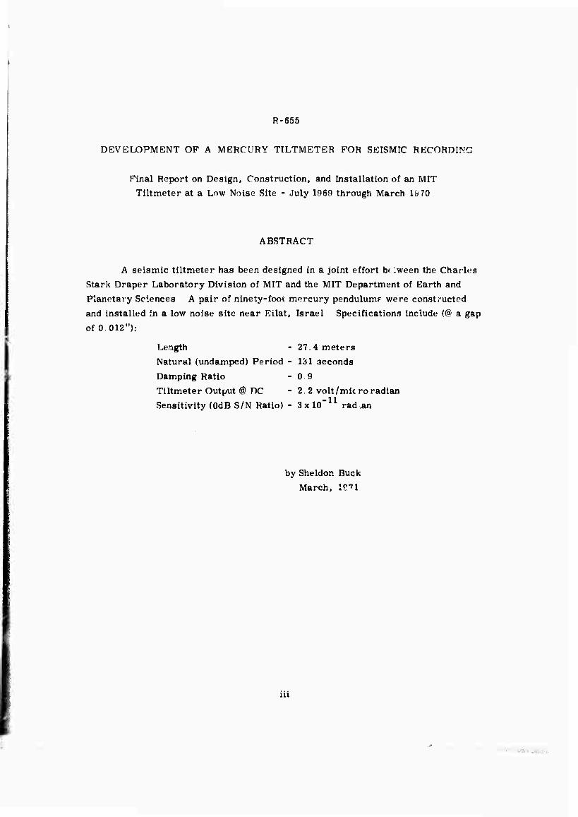
A seismic tiltmeter has been designed in a joint effort b( '.ween the Charles
Stark Draper Laboratory Division of MIT and the MIT Department of Earth and
Planetary Sciences A pair of ninety-foot mercury pendulum? were constructed
and installed in a low noise site near Eilat, Israel Specifications include (@ a gap
of 0.012"):
Length - 27.4 meters
Natural (undamped) Period - 131 seconds
Damping Ratio -0.9
Tiltmeter Output @ DC -2.2 volt/mic ro radian
Sensitivity (OdB S/N Ratio) - SxlO-11 radian
by Sheldon Buck
March, l?"n
iii
■. •■
R-655
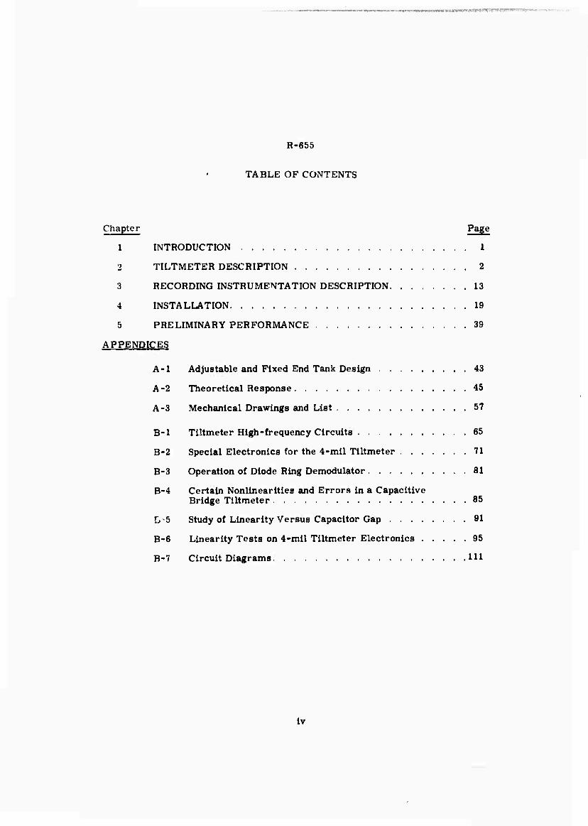
TABLE OF CONTENTS
Chapter Page
1 INTRODUCTION 1
2 TILTMETER DESCRIPTION 2
3 RECORDING INSTRUMENTATION DESCRIPTION 13
4 INSTALLATION 19
5 PRELIMINARY PERFORMANCE 39
APPENDICES
A-l Adjustable and Fixed End Tank Design 43
A-2 Theoretical Response 45
A-3 Mechanical Drawings and List 57
B-l Tiltmeter High-frequency Circuits 65
B-2 Special Electronics for the 4-mil Tiltmeter 71
B-3 Operation of Diode Ring Demodulator 81
B-4 Certain Nonlinearities and Errors in a Capacitive Bridge Tiltmeter 85
L5 Study of Linearity Versus Capacitor Gap 91
B-6 Linearity Tests on 4-mil Tiltmeter Electronics 95
B-7 Circuit Diagrams Ill
iv

■ ■
LIST OF ILLUSTRATIONS
Figure Page
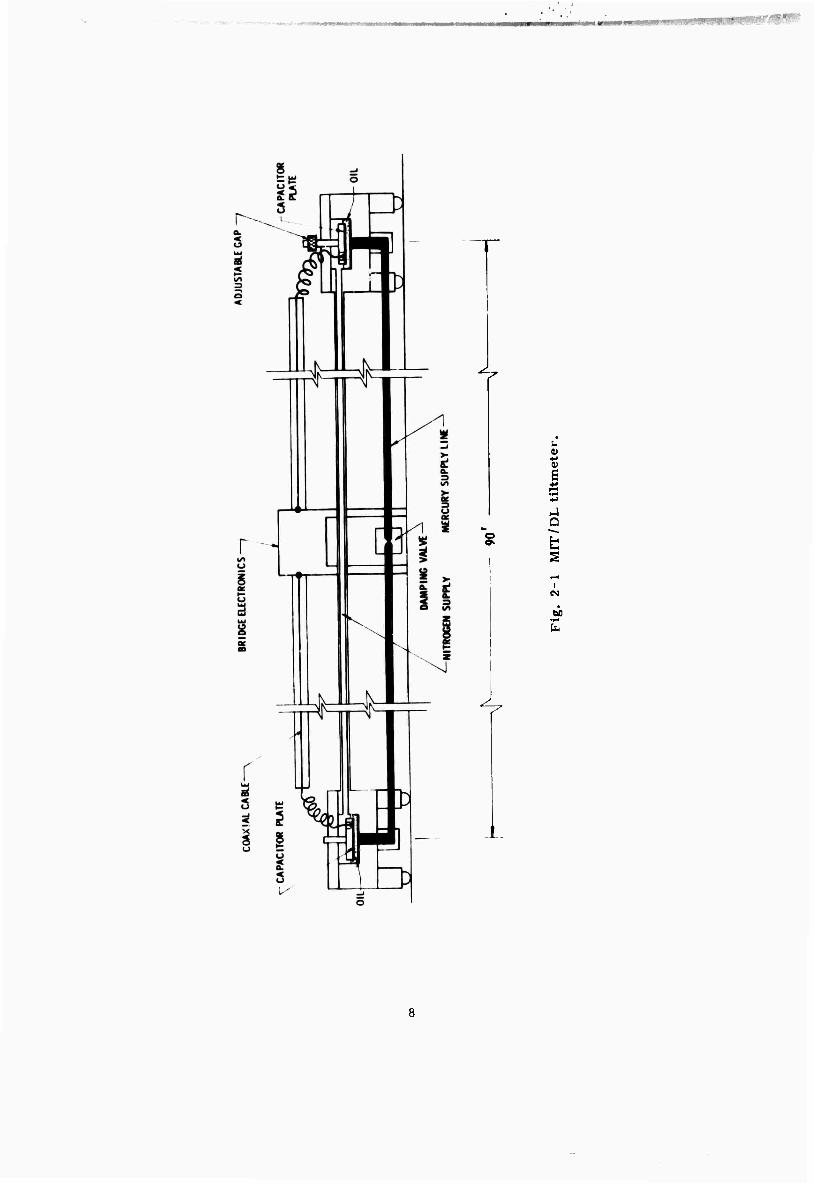
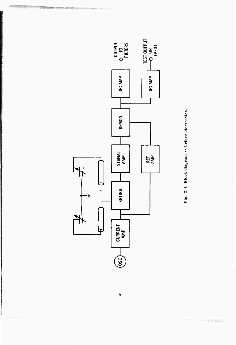
2-1 MIT DL tiltmeter 8 2-2 Block diagram — bridge electronics 9 2-3 Tiltmeter mechanical responses 10 2-4 Tilt mechanical gain 11 2-5 Displacement mechanical gain 12
3-1 MIT seismic station 15 3-2 Data channel filters 16 3-3 Differential temperature bridge calibration 17
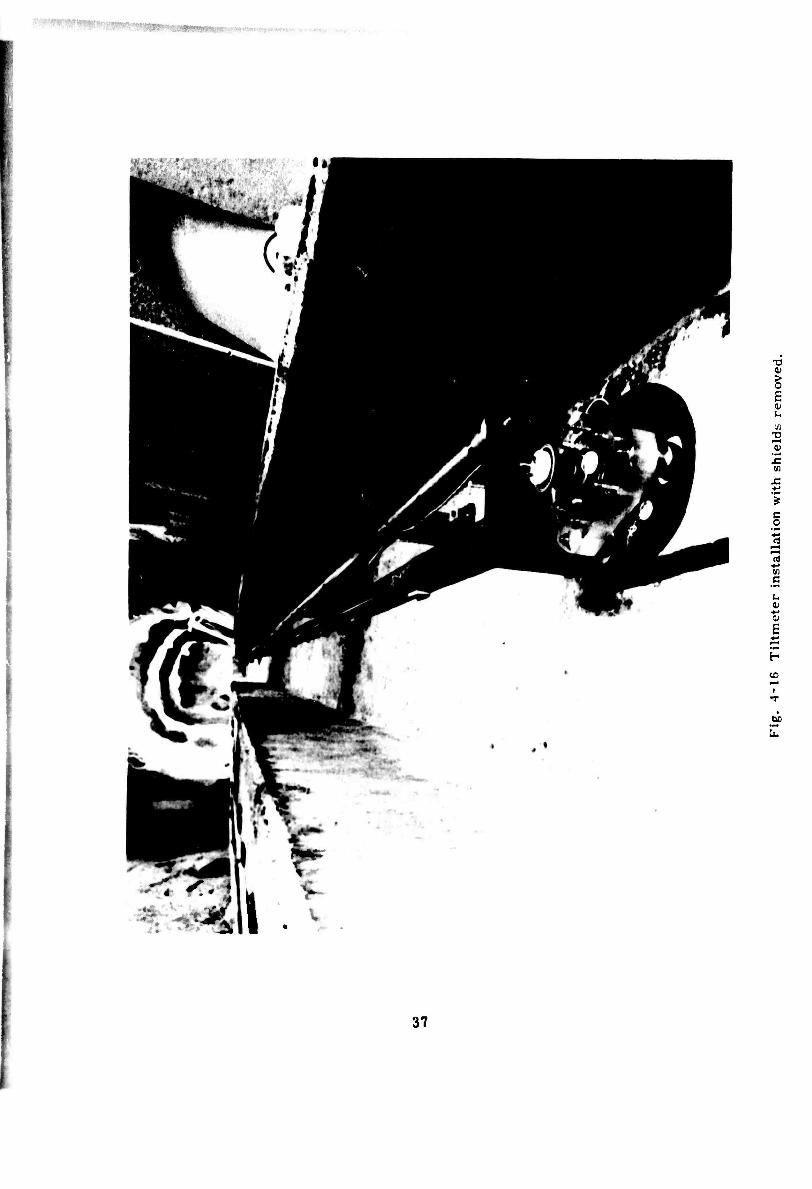
4-1 Plan of the Geophysical Observatory 22 4-2 Analog recording consoles 23 4-3 Tiltmeter showing mercury lines 24 4-4 Fixed end tank 25 4-5 Adjustable end tank 26 4-6 Electronic boxes 27 4-7 Bridge electronics — alignment panel 28 4-8 Bridge electronics — differential capacitance 29 4-9 Oscillator, power supply, and differential temperature 30 4-10 Filter networks — offset trims 31 4-11 Filter networks — control panel 32 4-12 Filter networks — tidal low pass filter 33 4-13 Filter networks — surface band pass filtei 34 4-14 Filter networks — eigen low pass filter 35 4-15 Filter networks — eigen high pass filter 36 4-16 Tiltmeter installation with shields removed 37
5-1 Surface wave records 40

Figure Page
A 2-1 Tiltmeter mechanical model 46 A. 2-2 Oil-filled capacitor , 51
A. 2-3 Root locus plot . 54
A. 3-1 Seismic tiltmeter — Mod II — installation 61
A. 3-2 Seismic tiltmeter - Mod II - layout 62
A. 3-3 Mercury chamber-fixed seismic tiltmeter — Mod II 63
A. 3-4 Mercury chamber-adjustable seismic tiltmeter-- Mod II. ... 64
B. 1-1 Tiltmeter high-frequency circuits 65
B. 1-2 Current amplifier 66
B. 1-3 Demodulator 68
B. 1-4 Capacitance bridge 69
B.2-1 Differential capacitance bridge 72
B.2-2 Current amplifier 74
B,2-3 Signal amplifier 77
B.2-4 AC reference amplifier 78
B.3-l(a) Demodulator 82
B. 3-l(b) Demodulator 82
B.3-l(c) Demodulator 83
B.3-l(d) Demodulator 83
B.4-1 Capacitive bridge tiltmeter 85
B.4-2 Bridge transformer 85
B.5-1 Bridge output versus gap 93
B.6-1 Test block diagram 95
B.6-2(a) Bridge output 98
B. 6-2(b) Bridge output 99
B. 6-2(c) Bridge output 100 B. 6-2(d) Bridge output 101
B 6-2(e) Bridge output 102
B.6-2(f) Bridge output 103 B.6-3 System linearity test diagram 104
B.6-4(a) Linearity test bridge electronics 105 B 6-4(b) Linearity test bridge electronics. . 106 B.6-4(c) Linearity test bridge electronics 107
VI

Figure Page
B.6-4(d) Linearity test bridge electronics 108 B. 6-4(e) Linearity test bridge electronics 109
B.7-1 MIT seismic station 112 B.7-2 System op-amps 113 B.7'3 Mercury tiltmeter bridge electronics 114 B.7-4 Bridge electronics — layout 115 B.7-5 Eigen filter 116 B.7-6 Eigen high pass — layout 117
B.7-7 Eigen low pass — layout. . . 118 B.7-8 Surface wave filter 119 B. 7-9 Surface wave filter — layout 120 B.7-10 Surface wave filter — line driver 121 B.7-11 Tidal filter 122
B. 7-12 Tidal filter - layout 123 B.7-13 Greenray crystal oscillator 124 B.7-14 Differential thermometer — schematic 125 B. 7-15 Differential thermometer—layout 126
vii
■■■■■■
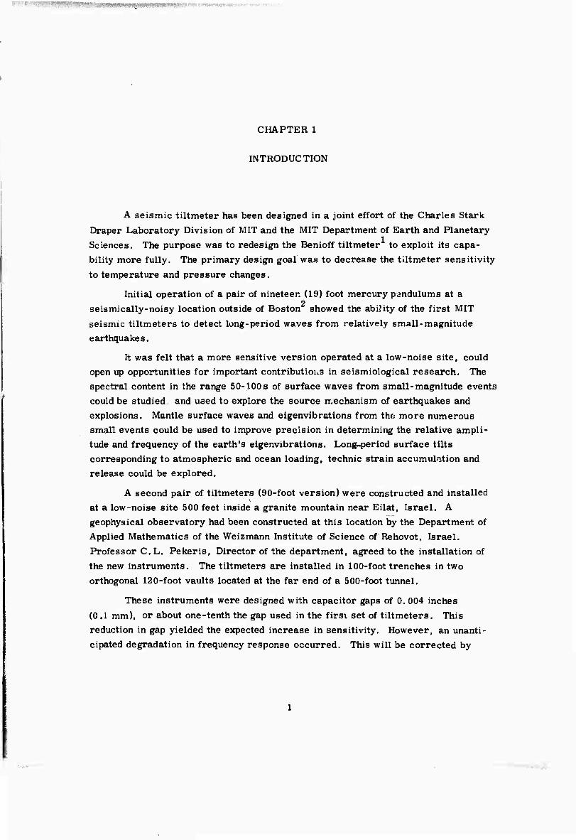
CHAPTER 1
INTRODUCTION
A seismic tiltmeter has been designed in a joint effort of the Charles Stark
Draper Laboratory Division of MIT and the MIT Department of Earth and Planetary
Sciences. The purpose was to redesign the Benioff tiltmeter to exploit its capa-
bility more fully. The primary design goal was to decrease the tiltmeter sensitivity
to temperature and pressure changes.
Initial operation of a pair of nineteen (19) foot mercury pendulums at a 2 seismically-noisy location outside of Boston showed the ability of the first MIT
seismic tiltmeters to detect long-period waves from relatively small-magnitude
earthquakes.
It was felt that a more sensitive version operated at a low-noise site, could open up opportunities for important contributious in seismiological research. The
spectral content in the range 50-100 s of surface waves from small-magnitude events
could be studied and used to explore the source mechanism of earthquakes and
explosions. Mantle surface waves and eigenvibrations from the; more numerous small events could be used to improve precision in determining the relative ampli-
tude and frequency of the earth's eigenvibrations. Long-period surface tilts corresponding to atmospheric and ocean loading, technic strain accumulation and
release could be explored.
A second pair of tiltmeters (90-foot version) were constructed and installed
at a low-noise site 500 feet inside a granite mountain near Eilat, Israel. A
geophysical observatory had been constructed at this location by the Department of
Applied Mathematics of the Weizmann Institute of Science of Rehovot, Israel.
Professor C. L. Pekeris, Director of the department, agreed to the installation of
the new instruments. The tiltmeters are installed in 100-foot trenches in two
orthogonal 120-foot vaults located at the far end of a 500-foot tunnel.
These instruments were designed with capacitor gaps of 0. 004 inches
(0.1 mm), or about one-tenth the gap used in the firsv set of tiltmeters. This
reduction in gap yielded the expected increase in sensitivity. However, an unanti-
cipated degradation in frequency response occurred. This will be corrected by

widening the gap threefold. This change can be accomplished without loss of
sensitivity since the gain can be recovered electronically.
At present, three output channels are producing data as follows:
1. Surface wave band, 16-120 seconds.
2. Mantle surface wave, eigenvibration band,
32-7200 seconds.
3. Permanent tilt and tidal band. 300 seconds to dc.
P PpWVi* ■■
CHAPTER 2
TILTMETER DESCRIPTION
General
Referring to Fig. 2-1, wo can sec that, like the seismic tiltmeter designed
by Huge Benioff and William Giles of the Seismnlogical Laboratory of California
Institute of Technology, the MIT mercury pendulum is formed by two end tanks at
opposite ends of the instrument and a connecting tube filled with mercury. An ai:
line filled with dry nitrogen is used to equalize the pressure over the mercury.
A differential-capacitance bridge with a capacitor plate over the mercury pool in
each end tank forms a differential mercury-level transducer while rejecting common-
mode changes in mercury level. An inert, stable transformer oil fills the gap
between the mercury pool surface and both the fixed and adjustable capacitor plates.
Besides providing additional protection against mercury oxidation, the oil prevents
the mercury from wetting and, hence, sticking to a capacitor plate in case of acci-
dental contact during assembly, adjustment, or instrument saturation due to very
large nearby earthquakes. Recovery from these disturbances is immediate,
except for the filter response. A second purpose of the insulating oil is to increase
the dielectric constant in the capacitor gap; thereby greatly increasing the ratio between the transducers' capacitance and the line capacitance of the 44-foot-long,
2-1/2 inch OD coaxial cable. The 1/4-inch ID connecting tube is made of butyrate in order to approximately match the thermal coefficient of expansion of mercury and
to provide a clear, transparent path between end tanks for checking the presence of
dirt or gas bubbles. The end tank structures are made of quartz for insulation and
mechanical stability. A differential screw-adjustment mechanism on one end tank
permits equalization of the capacitor plate gaps. The end tanks rest on a three-
point, non-redundant, strain-free base which prevents both stress and tilting of
the end tanks due to differential thermal expansion between the pier and end tank.
The relative plate gaps of the end tank capacitors are detected by a differ-
ential capacitance bridge. The scale factor change normally caused by a common-
mode gap change has been nearly eliminated by using a current source, instead of
the original voltage source, to excite the capacitance bridge. A block-diagram of
the bridge electronics is shown in Fig. 2-2. A 300-kHz crystal oscillator provides
the ac reference for the current amplifier driving the bridge transformer. A bridge transformer steps up the voltage from the current amplifier 10:1. One pair of secondaries forms two arms of an ac bridge circuit. The other two arms of the ac bridge are the capacitors of the adjustable and fixed end tanks, shunted by the capacity of the coaxial line. An auxiliary winding on the bridge transformer provides quadrature correction. The output of the ac bridge is amplified by an ac preamp having a feedback circuit tuned to the crystal oscillator for noise reduction. Amplified ac signals are converted to bipolar dc signals by a phase-sensitive demodu- lator which obtains Its reference from the primary of the bridge transformer. The phase-sensitive (diode ring) demodulator will rectify only signals coherent with the reference signal, thereby eliminating stray ac pickup. The dc signal is filtered and passed through a signal-conditioning amplifier for gain normalization and low output impedance. Two of these signal-conditioning amplifiers were used so that the bridge output could be monitored without disturbing the seismic and tidal filter networks connected to the primary output. Since the tiltmeter constitutes an open- loop system, all components must have high precision and stability, and all ampli- fiers must have negative feedback, for both gain stability and linearity. For a more detailed discussion of the linearity of the differential capacitance bridge, refer to Appendix B. 6. For linearity of the mercury pendulum, see Appendix A. 2.
Sensitivity
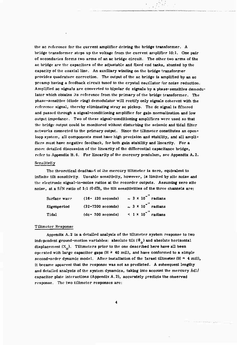
The theoretical deadbani of ihe mercury tiltmeter is zero, equivalent to infinite tilt sensitivity. Useable sensitivity, however, is limited by site noise and the electronic signal-to-noise ratios at the recorder outputs. Assuming zero site noise, at a S/N ratio of 1:1 (OdB), the tilt sensitivities of the three channels are:
Surface wave (16- 120 seconds) ~ 3 x 10 radians
Eigenperiod (32-7200 seconds) ~ 3 x 10" radians
Tidal (dc- 300 seconds) < 1 x 10" radians
Tiltmeter Response
Appendix A. 2 is a detailed analysis of the tiltmeter system response to two independent ground-motion variables: absolute tilt (9 ) and absolute horizontal displacement (X ). Tiltmeters prior to the one described here have all been operated with large capacitor gaps (H 2 40 mil), and have conformed to a simple second-order dynamic model. After installation of the Israel tiltmeter (H = 4 mil), it became apparent that the response was not as predicted. A subsequent lengthy and detailed analysis of the system dynamics, taking into account the mercury /oil/ capacitor plate interactions (Appendix A.2), accurately predicts the observed response. The two tiltmeter responses are:
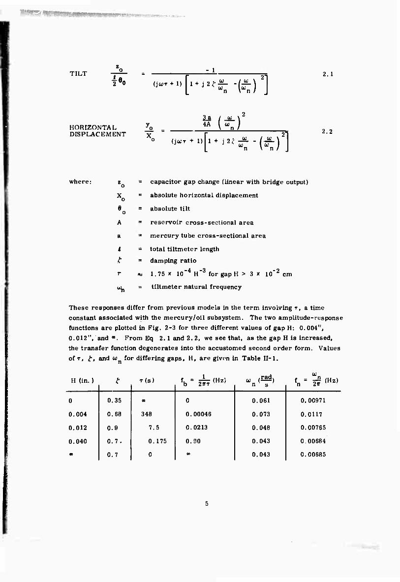
TILT i-e 20
- i 2.1
HORIZONTAL jo^ DISPLACEMENT x
la 4A (t)
(JOJT + 1) [1 + J2^-(t)2 2.2
where:
A
a
i
t r
- capacitor gap change (linear with bridge output)
= absolute horizontal displacement
= absolute tilt
= reservoir cross-sectional area
= mercury tube cross-sectional area
= total tiltmeter length
= damping ratio
M. 1.75 X 10"4 H*3 for gap H > 3 x 10"2 cm
di = tiltmeter natural frequency
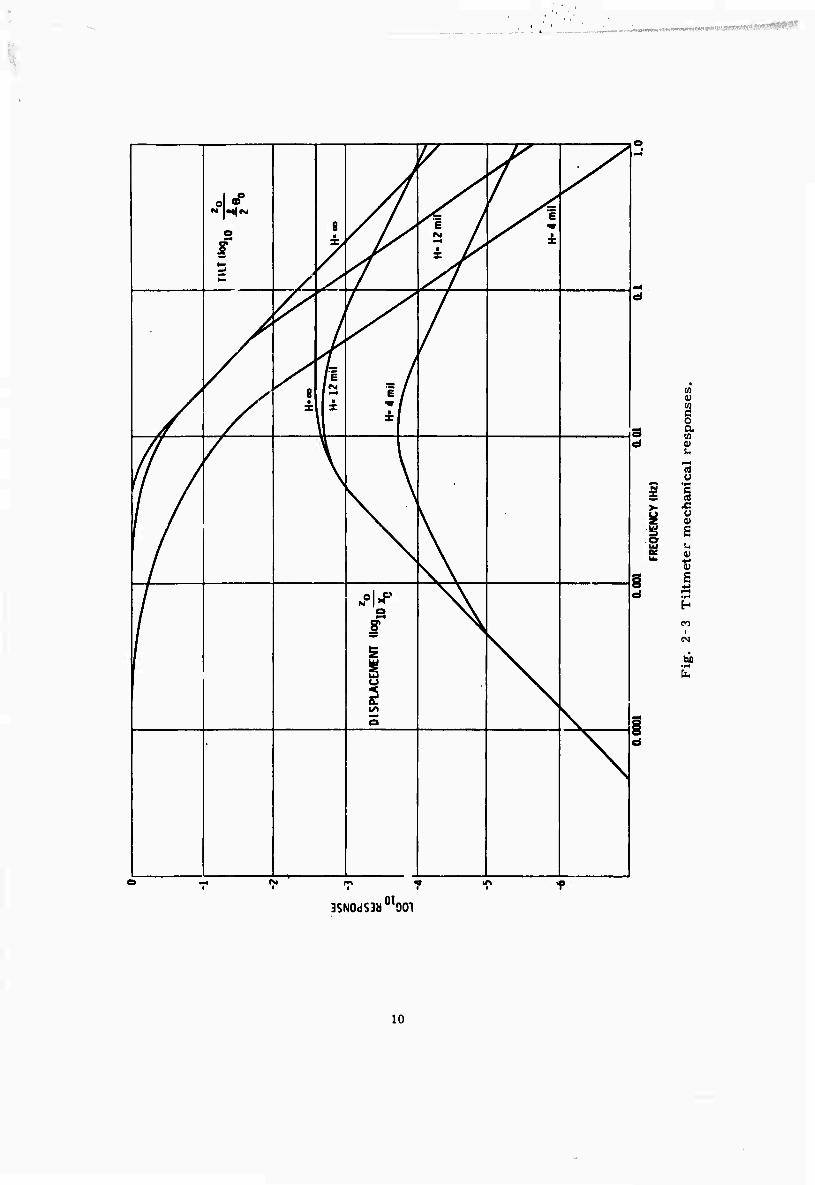
These responses differ from previous models in the term involving T, a time
constant associated with the mercury/oil subsystem. The two amplitude-response
functions are plotted in Fig. 2-3 for three different values of gap H: 0.004",
0.012", and ". From Eq 2.1 and 2.2, we see that, as the gap H is increased,
the transfer function degenerates into the accustomed second order form. Values
of T, if, and tu for differing gaps, H, are given in Table II-1.
H (in. ) ^ T(S) fb = L <Hz> n s fn = H (Hz>
0 0.35 00 0 0.061 0.00971
0.004 0.68 348 0.00046 0.073 0.0117
0.012 0.9 7.5 0.0213 0.048 0.00765
0.040 0.7. 0.175 0.90 0.043 0.00684
00 0.7 0 CD 0.043 0.00685
The ffft'ct of T is easily seen from the p!ots of Fig. 2-3. At small values of
II, the time constant T becomes la'ge enough to affect the dynamic response in the
region of interest. The response becomes third-order with the introduction of a
breakpoint, nnd urst-order rolloff at f, = T— , in addition to the usual second- r (jjn b 2ffT order- break at f - -srr. n 2ff
At n gap II of 0.004 in., both the tilt and displacement responses are down
> '^0 dB (^ 10) in the region 0.01-1 Hz. In addition, the response becomes
increasingly sensitive to common-i.iode changes in H. This is clearly undesirable in terms of instrument gain. From dynamic-response considerations alone, a gap
of II - x would seem to be the id.al. However, both bridge sensitivity and bridge
linearity are inverse functions of H. In view of all effects, the gap is being
lowered to what seems a best compromise, 0.012 in.
Mechanical Gain
Mechanical gain is an expression of recorder pen motion versus input ground
motion. A tiltmeter responds to two independent ground-motion variables,
absolute tilt (6 ) and absolute horizontal displacement (X ). We must therefore,
define two mechanical gains: tilt gain (in. /rad) and displacement gain (in. /in. ).
The mechanical gains in each data channel are found by the product:
tiltmeter response x filter response x recorder scale factor
The tiltmeter responses are shown in normalized form in Fig. 2-3.
The un-normalized responses for any specific gap, H, are determined by
assigning a precise number to a single point on the curves. This is easily and
precisely done by introducing a known tilt through the adjustable end tank and
observing the steadystate bridge output change. For the Israel tiltmeter. this
number has been determined as 6.67 volt/mlcroradian @ H = 0.004 in. The
mechanical gain figures given below assume this figure. For different values
of H, the tiltmeter scale factor changes, but it is assumed that this change will be
balanced by a complementary recorder scale-factor change.
The data channel filter responses and recorder scale factors are described
in more detail in Chapter 3. The filter amplitude responses are given in Fig. 3'2.
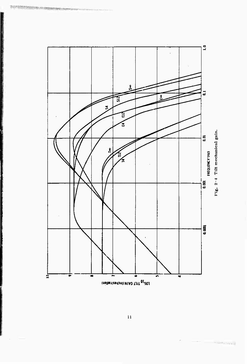
Tilt Gain
Tilt mechanical gain is shown in Fig. 2-4. The most serious degradation due to the 4-mil gap is in the surface wave channel where response is down ~ 18 dB
from the ideal throughout the band. The eigenresponse is down approximately 3 dB
(x 0. 7) at an 18-minute period. The tidal band is not seriously affected. By

increasing the gap to 0.012 in., we approach the ideal to within 2 dB(x 0.8) over
all regions of interest.
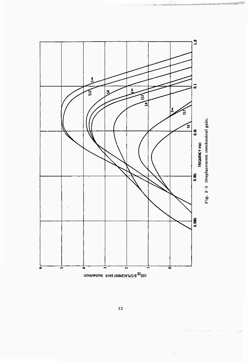
Displacement Gain
Displacement mechanical gain is shown in Fig. 2-5. The percentage degrada-
tions in the various frequency bands are identical to those in tilt gain. This is a
result of the identical tilt and displacment transfer function denominators. One
significant improvement which would result from opening the gap to > 0.012 in.
would be a flatter amplitude response in the surface wave band of 16 - 120 seconds.
o Q
E I
(N
U)
^
9<*e^T..
¥
OU
TPU
T
O
TO
FILT
ER
S
TEST
OU
TPU
O O
R
(A-D
)
CL
< u o D
C A
MP
1
o
o
• w Ü
•fMl
c 0 u t a,
l-H 4)
01 be
T3
u
k
SIG
NA
L
AM
P u.a.
UJ S
Si
1 1
g
M •**
U 0
1—t
< Hi'
r I
UJ O O
P3
1 CM
mJ
CU
RR
EN
T A
MP
(k)
i
ummiiTiirm IIIM«IIIIMIIW ,-,.,■,.■.'>.■:- ^■1.^, ■ ■ ■"■■'■■■ '
J ^ /
-■
/
8 H m*
/ <y i /x <*
/
/
X i 1 I
1 X I l/
/ \\ n
V V N\ L
et
\ 1 \ §
e'
s f \
i
a \
\
e(
* * f " * f ^ P
(0
u
Ü
ü
£
CO
3SNOdS3a0,9O1
10
■ ■ ■ .
:
8
J /
/
^^ UJ
8 ^^-ii
^
V \
/^v \
/
^ /k
/ ^ \
(
\
\
\
\
\
\
\
\
bo
rt o
•r-
i r- 0 > 0) ^ F UJ 3 O «
8 i
CM
•r«
|Ul|pCJ/s*M3U|) Nl VO nil O,«)01
11
.■..-.: '■--■■' ■■»":■■,
8 ^
^ ^
(
S! i^-^
^^a- ^^-^s
^
V i d Ö /*
^ H
.3 (A M
i—i a) o
i "
| %
^ e u n)
8 in «* s
in i
(N
E
(ipu|/s»M3U!) NIVO iN3W3DV1dSia 01001
12

CHAPTER 3
RECORDING INSTRUMENTATION DESCRIPTION
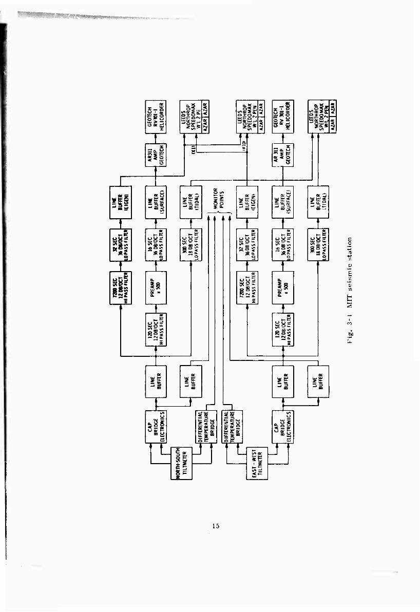
Outputs of the MIT seismic tiltmeters are recorded on both chart and drum analog recorders. The output of each tiltmeter passes through one low-pass and
two bandpass filters. A block diagram of the recording instrumentation at the
Weizmann Geophysical Observatory is shown in Fig. 3-1. Figure 3-2 gives the
amplitude responses of the three filter channels.
The low-pass filter was designed to isolate earth tides and long-term drift. The two bandpass filters were designed for emphasis of (a) eigenperiod on free-
mode oscillations of the earth, and (b) surface waves in the region 0. 5 - 4 cycles per minute for explosion versus earthquake discrimination.
The tidal filter is an active third-order Butterworth low-pass with a break-
point at 300 seconds and a rolloff of -18 dB/octave. It has unity gain in the pass- band and an optimally flat amplitude response.
The eigenperiod filter consists of an active second-order high-pass section
with a breakpoint at 7200 seconds and rolloff of -12 dB/octave and two cascaded
third-order Butterworth low-pass sections with breakpoints at 32 seconds and
combined rolloff of -36 dB/octave.
The surface-wave filter consists of an active second-order high-pass section
with a 120-second breakpoint and -12 dB/octave rolloff, followed by a chopper-
stabilized preamp with a gain of 500, followed by two cascaded active third-order
Butterworth low-pass sections with breakpoints at 16 seconds and combined rolloff
of -36dB/octave.
Leeds and Northrup Speedomax W/L 2 pen, 10-inch chart recorders are used
to record the outputs of the earth tide and eigenperiod filter networks. The earth
tide recorder runs at a chart speed of 4 inches per hour and a full-scale span of 2
volts. The eigenperiod recorder runs at a chart speed of 15 inches per hour and a
full-scale span of 100 millivolts.
The L&N chart recorders have built-in AZAR units for zero pen position
(bias) and full-scale span (range or scale factor) adjustments.
13
:■
■

Geotech drum recorders (Model RV301-1 Helicorder) are used for recording
surface waves. The drum speed is 1 revolution per hour, and the stylus traverses the drum at the rate of 3/8 in. per hour. The helicorders have been modified with
rectilinear pens which, when driven with Geotech AR311 amplifiers, have a scale
factor of 0. 05 volts/in. @ OdB. The solid-state helicorders are very stable and have
a good signal-to-noise ratio.
Line buffers or drive amplifiers were incorporated in all filter output
channels. Besides providing low output impedance, these line buffers incorporated
special feedback compensation for stable operation with 800-foot signal cables with
a 2000-pF capacitance. The signal cables were shielded, twisted-pair, two- conductor microphone cables.
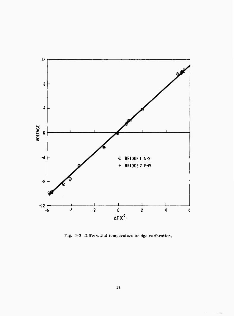
Differential Temperature Bridges
Since the tiltmeter is sensitive to horizontal ambient temperature gradients, differential temperature bridges were provided for each tiltmeter, with the resistive probes located at the end tanks. Compensation for gradients was originally
contemplated, but the effects of such gradients in the Weizman Observatory have thus far been insignificantly small. Figure 3-3 is a calibration of the two bridges.
14
O K ÜJ
t X
m s fci 2« o
ill -'S a
uj O w
<o O i^t
S
l§
I tt 0 1_)
B UJ O
R g I
si
I <J tt <-
0.5
UJ ►— O CSi UJQ^ UJ _. -JQUJ--'
0.5 «
'acuj-< a-a.«
UJ UJ ^ Z u- 5 „ u- O
n if A
MM
(j <-> ii UJ O u
s 2 "^ o
2 2
xr§
o > — 0«!
£ u- O ■-25
1-K UJ O u.
INI S ^ " 2 «
g
"D is
« * e
5 tu TT
I S a. <->
oc < o
a: o
= 95
o X- UJ W U-
o
Ö 5
CA
P
BR
IDG
E EL
ECTR
ON
ICS
" L J ■ ■ s -
u?!
zo.« t/1
*|s
0 v =; uj O w
^ ao a, "* o
C _C
<-> M
O
£ 'S
or IB
15

<$
^^^^^^ r w * j^r
^r
H N k
N
n N < o
\
\
f\
k
09
X ü
o 5 3 CO 5 IS
S
I M l
«NJ IT.
,01 901) N0liVnN3UV
16
12
o >
-4 -
-8 -
© BRIDGE 1 N-S
+ BRIDGE 2 E-W
-12 -4
AT (C0)
Fig. 3-3 Differential temperature bridge calibration.
17
-

BLANK PAGE
7
CHAPTER 4
INSTALLATION
Installation of the Model II MIT seismic tiltmeter took place near Eilat, Israel, during the months of May and June, 1970. After completing the instrument fabrication work, the end tank subassemblies, electronic field cases, recording consoles, and other equipments were crated and otherwise prepared for air freight to Lod airport near Tel Aviv, Israel. On April 22, 4,800 pounds of equipment, working tools and test instruments left the United States for Israel.
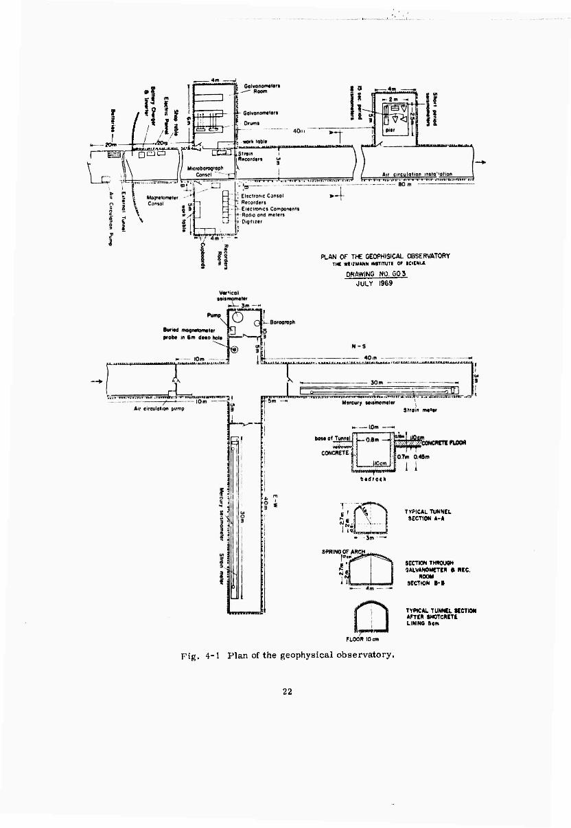
The 90-foot mercury pendulums are installed in orthogonal trenches located over 500 feet inside a granite mountain just north of Eilat, near the Timna copper mines. A plan of this geophysical observatory of the Weizmann Institute of Science is shown in Fig. 4-1. The instrument tunnels are lined with gunite or shot- crete, and are pressure-sealed with bulkhead doors. The environment of these sealed tunnels is nearly a constant 118 F, or 480C, with a relative humidity vary- ing from 90 to 100%.
The first instillation task was the installation of recording equipment. One of the Leeds & Northrop servo amplifiers burned out because of a heat-sink bracket which loosened during shipment, causing a short circuit. The three L & N W/L II 10-inch chart recorders are installed in an enclosed 19-inch console along with three AZAR (adjustable zero/adjustable range) units. Initially, one of these two channel recorders was used for recording earth tides, one for eigen- periods, and one for differential temperature. Eventually, two recorders will be
used for eigenperiods at different gain settings.
The drum "Hellcorders", along with their drive amplifiers, were mounted in a second 19-inch console. Initially, there was a problem with the pen heater control circuit because of the elevated operating temperatures.
Timing signals for both recording consoles were derived from the observa- tory's time standard, which is checked oach day and synchronized whenever necessary. An air conditioner is now providing cool air in the recording room; this has greatly reduced overheating of the recording equipment electronics and motors. Fig. 4-2 is a photograph of the drum and chart recording consoles.
19

The next task was to prepare the trenches for installation of the tiltmeters.
Four sets of three conical holes were drilled in the trench end tank piers. These
precisely-located conical holes were made with special carbide drills and counter-
sinks, and held the one-inch stainless steel balls used to support the end tank
assemblies. Then, the bases of the aluminum end taiitc shields were grouted in place.
The four 45-foot, 2 1/2-inch diameter, coaxial lines were assembled, using
li-foot sections except for the end. A continuous length of #18 Teflon-coated wire
was used as a center conductor, while 2 1/2-inch diameter copper tubing was
used as an outer conductor. Brass couplings with O-ring seals were used to join
the 12-foot sections. Problems were encountered because of damage and distortion
of the copper tubing during shipment. The assembly of the coaxial lines, including
the installation in the trenches and fitting with the junction boxes, took about one
week.
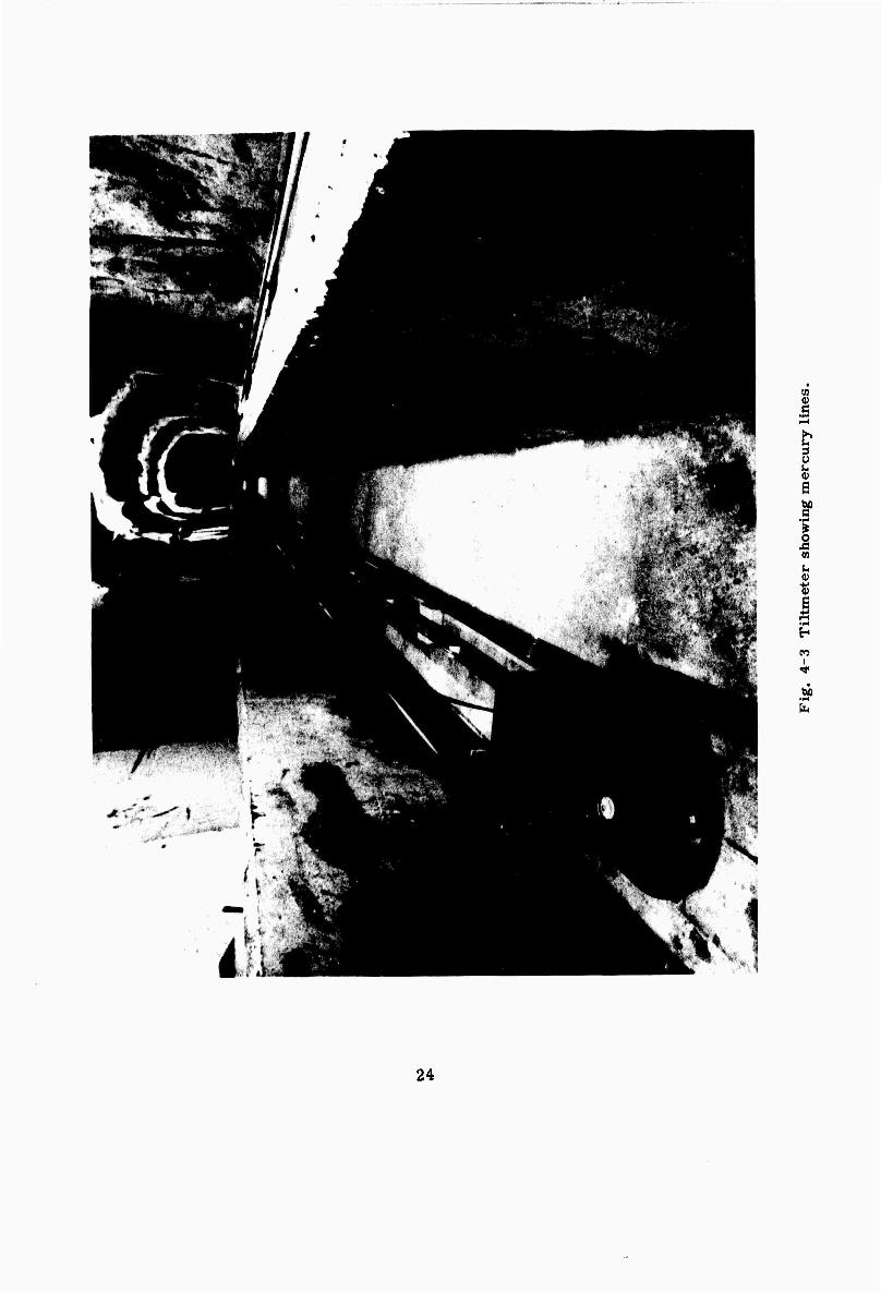
Aluminum heat shields were installed to protect the l/4"-ID, 3/8"-OD
butyrate plastic tubing used as a mercury line between end tanks. Butyrate tubing
was selected because it was clear, semi-rigid, and approximately matched the
thermr.l expansion of mercury. However, the matching of thermal expansion with mercury, which worked out well at the Agassiz (Harvard, Mass.) installation, did
not hold for the Weizmann installation. Apparently, at the higher operating temperature (118 F) the plastic expands even more than the mercury. Also, the
increase in nitrogen pressure with temperature in the completely sealed instru-
ment added to the problem. A photograph of a tiltmeter with the mercury line
exposed is shown in Fig. 4-3.
The nitrogen lines (1/8" ID, 1/4" OD) between end tanks were installed next,
and secured to and supported by the coaxial lines.
The adjustable and fixed end tanks were installed and leveled. The require- ment for a better leveling fixture became apparent, and has since been designed and
built. The end tank leveling and relative elevation is controlled by adjustment
shims in the end tank supports. The leveling procedure proved very time-
consuming, but seems to provide for very stable end tanks once adjusted.
The two tiltmeters were filled with mercury. Trouble was immediately
encountered with the first instrument (North-South) beca ise of mercury oxida- tion. This mercury surface contamination may have been caused by dirt in the
mercury floating to the surface, or oxidation caused by lack of proper purging of
the instrument with nitrogen before filling. The South end tank was opened, drained,
cleaned, and refilled. Mercury from a new shipment was used in filling the East-
West tiltmeter, along with continuous nitrogen purging. A different filling technique
20

helped prevent bubbles from entering the mercury lines. No trouble was encoun- tered in filling the East-West instrument, and the end tank surfaces appeared very clean.
The fixed end tank capacitor plates were adjusted to 0.004-inch, or 0.1- millimeter gap, by the use of shims. At this small clearance, a short circuit occurred in the South end tank, which was then opened for inspection. No suspec- ted floating metal particle was found. The South end tank was reassembled. Capacitance readings of 2000 picofarads were obtained, indicating the proper 0.004-inch gap, but a high dissipation factor would occasionally show. Again, no trouble whatsoever was found in the West end tank. One of the fixed end tanks is shown in Fig. 4-4.
The adjustable end tank gaps were made equal to the fixed end tank gaps by means of the differential screw adjustment. One turn of the screw equals 0 .0009 inches, or 0.023 mm, so no trouble was encountered in achieving a balanced capacitor plate clearance. A tapered collet nut provided a means of eliminating the backlash on each of the two threads on the differential screw. Some backlash remained after final tightening, but it was small enough to be compi nsated for. One of the adjustable end tanks is shown in Fig. 4-5.
As the room temperature rose after sealing the tunnel, the mercury level dropped in the end tanks, i.e., the capacitor plate gaps increased. This change in mercury level was easily compensated by injecting more mercury into the mercury line with a syringe. The mercury-level syringe is adjusted with a micro- meter located at the center of each instrument, in front of the junction box. A photograph of the syringe/micrometer, junction box, bridge electronics, and filter network field cases is shown as Fig. 4-6.
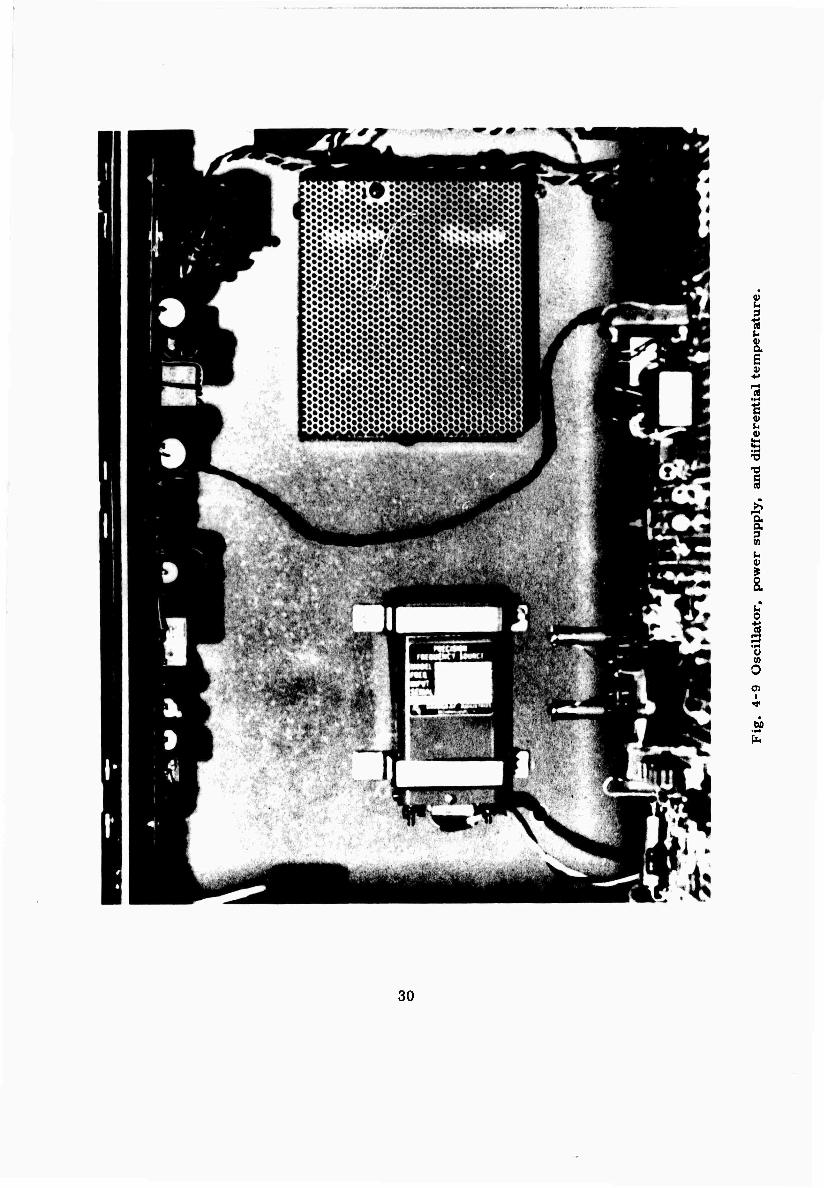
The bridge electronics box was installed and the differential capacitance bridge nulled, quadrature trimmed, and amplifiers tuned after the capacitor plates were adjusted. The bridge circuits are described and analyzed in detail in Appendix B.2. Photographs of the differential capacitance bridge, along with its oscillator or ac reference and power supply, and the differential temperature bridge are shown in Fig. 4-7,8,9. No trouble was encountered in tuning or trimming after power supply warmup.
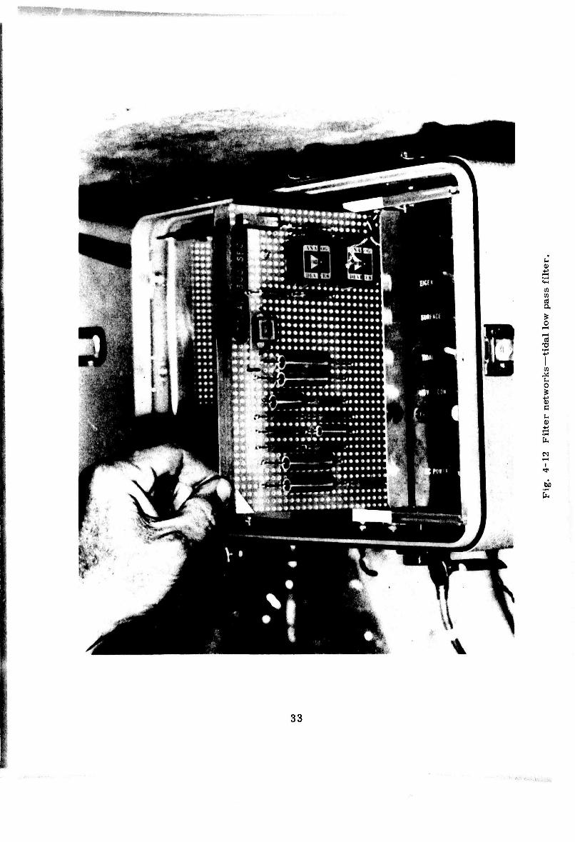
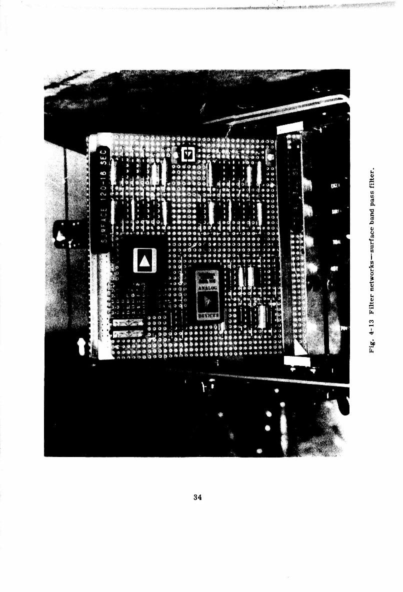
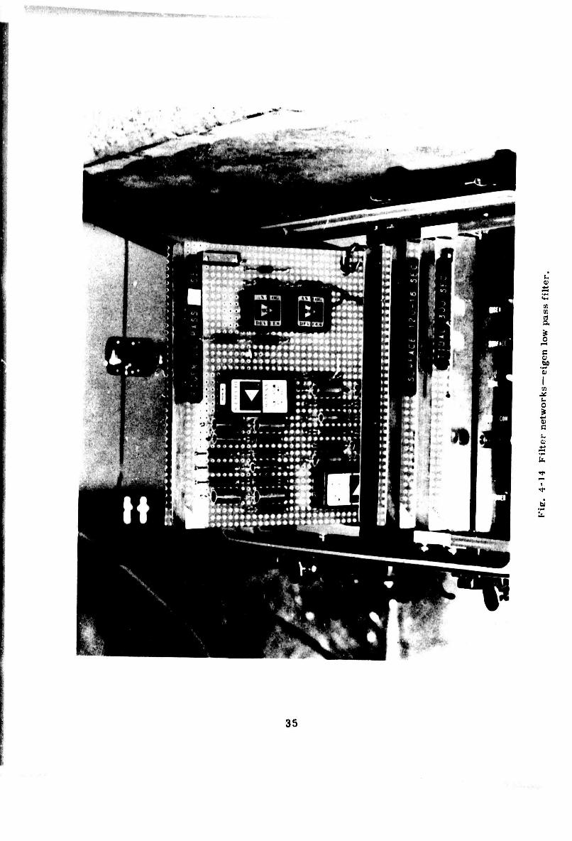
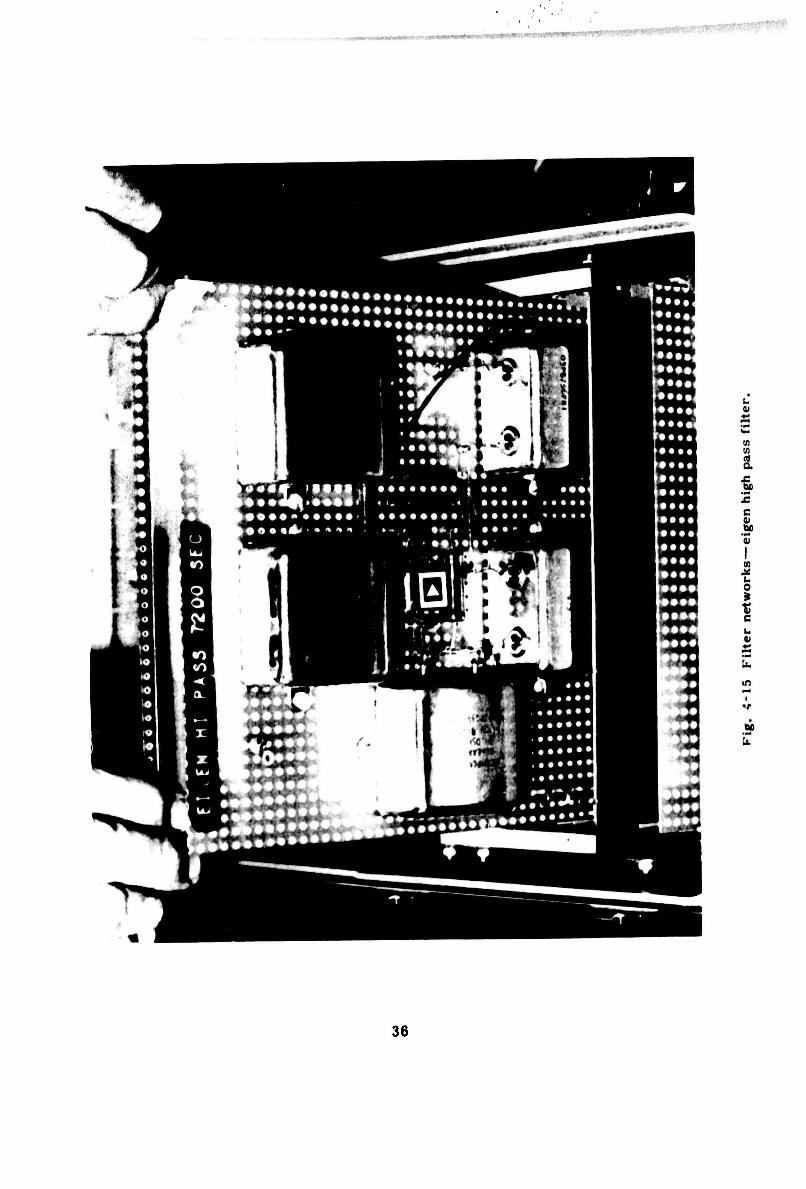
Next, the filter networks were installed, adjusted and calibrated before connection to the bridge electronics. The input voltage bias trim to the gain-of- 500 amplifier between the high-and low-pass sections of the surface-wave filter required readjustment due to the great temperature change. Otherwise, all circuits showed low noise, stable outputs, and performance as expected. Photo-
graphs of the tidal, surface, and eigennetworks, including detailed construction, are shown in Fig. 4-10, 11, 12, 13, 14, and 15. The completed tiltmeter, with end
tank shields removed, is shown in Fig. 4-16.
21
I i'Kilm
PLAN OF THE GEOPHISICAL OBSERVATORY THE «EIIMANN INSTITUTE OP SCIENUl
DRAWING NO GO 3 JULY 1969
-lOm ' Atr circulation pump |3 Strain mittr
btdrock
■• 3tn-
SPRINOOFARCH Itftm
TYPICAL TUNNEL SECTION A-A
SECTION THROUOH SALVANOMETER 0 HCC.
ROOM SECTION B-B
TYPICAL TUNNEL SECTION AFTER SHOTCRETK LINING Sen
FLOOR 10 cm
Fig. 4-1 Plan of the geophysical observatory.
22
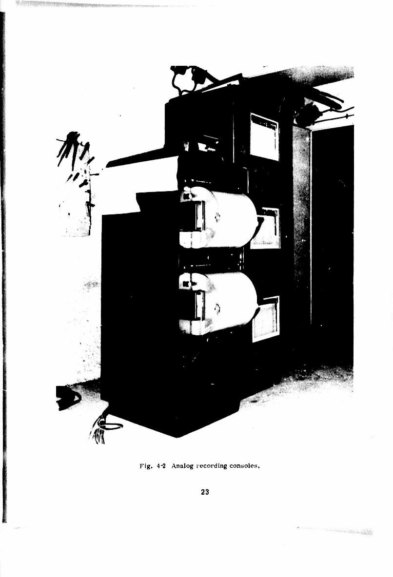
Fig. 4-2 Analog recording consoles.
23
10 0) c
u 3 u u 0)
be c
X! (0
u
% £
I
tÜD
24

c •v
i
25

I c 0)
in i
tfH
26

in
§ JD
g o HI
s CO
I f
tu
2'.

t
•3 a) V
0)
•i-i
vlD
lb
28

*nmw*Vfi*iW~ • '
01 ü c
+» o n) a m u
c a> u 0)
I o c 0
be
CO
ao I t
M
29
<u u
u a E
i- 0)
T3
to
4)
O a
o
l-H •H u (0 0
I
30

(A
£ t a;
o
c
4)
o
bo
31

gga iii^wiMi—WP^—^w
0) c n) a o
I Ü
to X u o
c
0)
I
32
0)
tn tn
a is o
T3
O
c
0)
fe
N
bo
33
■
■ ■ -■ ■■'',-■■ II'-.-. mmmmm^^mm.
u (U
tn
a
0) ü nl U 3 (fl
CO X U 0
X a u i)
C5
34
I ^...;» .; .,,
v. t I c
«3
U o
« c u QJ
35
mmmmrnmrnwrp-
36
•
XI 0)
E <v u ■J.
-a
Efl
c —
01
E Ä H
r
37

■^r^ -~
I
r ■ü i i i
...... ■ ■■,■ -.. . ■ .. ....
CHAPTER 5
PRELIMINARY PERFORMANCE
As of this writing, about three months of records are available to assess the
performance of the tiltmeters installed in Eilat, This is not yet a sufficient suite
of records to achieve the research goals referred to earlier, but it does provide
preliminary indications on the performance of the instruments.
An examination of the records indicates that in the surface-wave band the
instruments are operating near the maximum sensitivity permitted by the ground
noise characteristic of the winter months. Widening the gap of the transducer capaci-
tance will lead to some improvement in performance in the winter months, and to a
marked improvement in the summer and on quiet winter days. The surface wave channel should be markedly improved by this modification.
The records differ from conventional seismographs in showing mantle
surface waves from relatively small events. We have not been able to Identify
most of these events because their magnitudes are too small to be reported through
usual channels. In further studies, we will track these tremors down in order to
study the efficiency of long wave excitation in the magnitude range less than 5
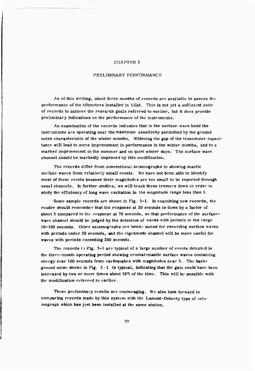
Some sample records arc shown in Fig. 5-1. In examining new records, the
reader should remember that the response at 20 seconds is down by a factor of
about 5 compared to the response at 70 seconds, so that performance of the surface-
wave channel should be judged by the detection of waves with periods in the range
50-100 seconds. Other seismographs are better suited for recording surface waves
with periods under 30 seconds, and the eigenmode channel will be more useful for
waves with periods exceeding 200 seconds.
The records ii Fig, 5-1 are typical of a large number of events detected in
the three-month operating period showing crustal-mantle surface waves containing
energy near 100 seconds from earthquakes with magnitudes near 5. The back-
ground noise shown in Fig. 5-1 is typical, indicating that the gain could have been
increased by two or more times about SO1"« of the time. This will be possible with
the modification referred to earlier.
These preliminary results are encouraging. We also look forward to
comparing records made by this system with the Lamont-Doherty type of seis-
mograph which has Just been installed at the same station.
:i!t
(1)
Record 1. Prince Edward Island. M = 5, 1, A = 75 . Showing excitation
aO-second surface waves on E-W component.
(2)
Hecord 2. California. M«5.4. A » 110 . Showing excitation of
100-second surface waves on N-S component.
(3)
Record i. Jun Magen Island. M ■ 5, 1. A« 47 . Showing excitation
of HO-second surface waves on E-W component
Flg. ü-1 Surface wave records
40

■
Record 4, 5. Large Soviet underground explosion 14 October 1970
on E-W (4) and N-S (5) components, maximum period
about 60 seconds.
Fig. 5-1 Surface wave records (continued).
41

•nr"™«'—''"« ^..m kn,m, ■ HI .iiiiiiii.i[iii.Mi..:,iiiiiii.j'iiiiii ii'iwwiiiilwpwPiiiNiiiiiiiiiiii'ia.ayiylllgl
W
i m -#*- ■•«•>

■;■„ ■■■■-: . ■ ■
APPENDIX A.l
ADJUSTABLE AND FKED END TANK DESIGN
The two end tank assemblies are very similar except for the manner in which the capacitor plates are positioned. The end tanks of the fi -st pair of tilt- meters were fabricated from Pyrex 10-inch diameter Pyrex lens blank. The end tanks for the second pair of tiltmeters were made entirely from quartz. Pyrex is probably the best material for the end tanks, as it is inexpensive, has consistent quality with uniform properties, is readily available, and grinds or machines well. Quartz, unless it is of select grade and highest quality, has been found to be of variable quantity, with sometimes severe bubble and dirt contamination, and is difficult to machine because of high internal stresses. The problems encountered in using quartz can only be overcome with a higher grade of material, which is much more expensive than Pyrex. Pyrex is sufficient for the application, since the optical properties and extremely low thermal coefficient of expansion of quartz are not needed. Plexiglas and other plastics were not used in end tank construction due to their mechanical instability and thermal hysteresis. Metals such as 316 stainless steel were not used because of the introduction of additional stray capa- citance and contamination of the mercury surface from amalgamation. Experience with manometers and other mercury-filled devices has shown that clean, polished glass and mercury have the most uniform wetting action.
The problem of providing a stable support for the end tank, while allowing for relative expansion with respect to the concrete piers, was solved by using a non-redundant, three-point design. (See Fig. A. 3-1 —4.) Three ball joints with fixed, V-grooved (1 degree of freedom), and flat plate (2 degrees of freedom) provide a self-aligning system free of any stresses save friction between the lapped V-groove and flat plate surfaces. Friction is minimized through hard- lapped surfaces and a special chromium coating (electrolizing). The end tanks are leveled with ground washers and shims between the support feet and the end tanks.
The end tanks are hermetically scaled with silicone-impregnated O-rings and epoxy Joints. A sealed system is necessary to prevent mercury oxidation and
condensation of water vapor.
43
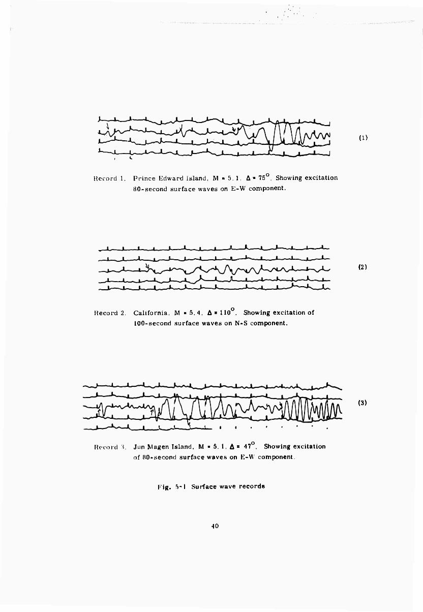
Tho capacitor plate is in the shape of a ring. The center hole minimizes
damping, and avoids the mercury entrance fitting at the bottom of the end tank.
The capacitor plate is a stainless steel ring, ground for flatness and chromium-
coated for1 corrosion resistance. It is attached on the adjusting shaft by means of
a quartz disk which acts as a mechanically-stable insulator. A single-path
electrical connection is made between the capacitor plate and a BNC fitting.
In the adjustable end tank (Pig. 4-5), the capacitor plate is moved vertically
by a differential screw mechanism. The differential screw is made of two
opposing threads: one with 46 threads per inch and the other with 48 threads per
inch. Since one screw advances while the second screw retracts, the resulting
combined motion provides a vertical adjustment of 0.0009 inches per turn.
The threads are lapped, hardened, relapped, and lubricated to minimize
friction (adjustment torque). One of each of the mating threads employs a split
collar and tapered collet, with a tapered nut to minimize thread play or backlash.
The middle or floating shaft (containing both threads) has a knurled knob which
insulates the hand when making a capacitor gap adjustment. The capacitor plate
does not rotate with respect to the end tank while moving vertically, making electri-
cal connection and sealing simpler. The differential screw has an adjustment
range of 44 turns, equivalent to ± 0.02 inches. A dial indicator provides a refer- ence for partial turns.
44
IP^M^' ■
APPENDIX A. 2
THEORETICAL RESPONSE OF THE TILTMETER
Part I; Simple Tiltmeter Dynamics
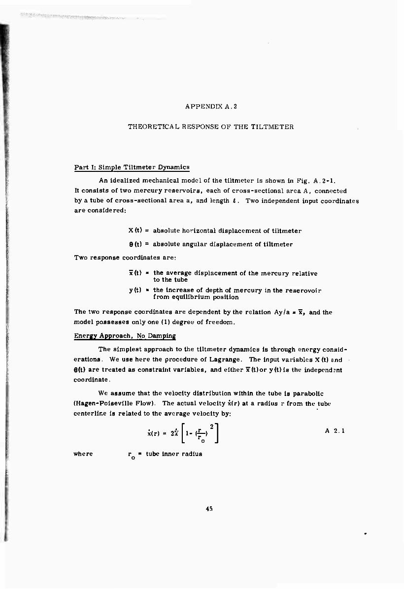
An idealized mechanical model of the tiltmeter is shown in Fig. A, 2-1.
It consists of two mercury reservoirs, each of cross-sectional area A, connected
by a tube of cross-sectional area a, and length I. Two independent input coordinates
are considered:
X (t) = absolute horizontal displacement of tiltmeter
6 (t) = absolute angular displacement of tiltmeter
Two response coordinates are:
x(t) ■ the average displacement of the mercury relative to the tube
y(t) ■ the increase of depth of mercury in the reserovoir from equilibrium position
The two response coordinates are dependent by the relation Ay/a ■ x, and the
model possesses only one (1) degree of freedom.
Energy Approach, No Damping
The simplest approach to the tiltmeter dynamics is through energy consid-
erations. We use here the procedure of Lagrange. The input variables X (t) end
Oft) are treated as constraint variables, and either x(t)or y(t)i3 the independent
coordinate.
We assume that the velocity distribution within the tube is parabolic
(Hagen-Poiseville Flow). The actual velocity x(r) at a radius r from the tube
centerline is related to the average velocity by:
j((r) 2x ' * ^ ' A 2.1 *K'2] where r ■ tube inner radius o
45

a)
AREA a
b) CAPACITOR PLATE ^y Fig. A.2-1 Tiltmeter mechanical model.
46

The kinetic energy of the tube mercury is then r
Ttube " 2 [A ^^ /2] e2 + 7 /0 ^2ffrdrl)[x + x(r)]2 A.2.2
Integrating,
T tube
The kinetic energies of the reservoirs are:
-ffi r^(ie)2 + X2*2*X + f J2] A.2.3
Tleftres = T [pAfh-y) ] [(^ + y)' + i'] A. 2.4
Trightres = I [^(h.y) ] [(^ + y)' + *] A.2.5
Since we are considering only the linear approximation for small motions, we • • •
consider only terms up to the second order in X, x, and 6. The total kinetic energy relation is therefore:
1 2 (jaL+M)aS)2 + (m + 2M)X2
+i£iiÜ+ 2MI ey 12 2
3 a' L 2 m'A' J
A.2.6
VfY\CVG m - pa 1, mass of tube mercury
.' = p Ah, mass of reservoir mercury
Representative values are m ^ 0 C^-O4]
j ~ 0 [0.0035]
9 3 M a " Therefore the term s— (x) niay be dropped with respect to unity
Wo next consider the potential energy. The potential energy changes are:
right reservoir; + p A h g -^ ••• pAygf-*^* y) A 2.7
1 6 left reservoir; - p A (h-y) g -7- A 2,8
47
The not change in potential energy is
V(y. 9) = p A gy [i6 + y)j A.2.9
Kint-tic and potential energies are combined to form the Lagrangian L ■ T-V, and
the equation of motion follows directly from the Lagrange equation
4 dt [n] -1*=» A.2.10
Since we have not considered damping, all forces are conservative. In standard form the y equation is
2 4f (A) y + (2pAg)y=-i2AX-pAg4e -Mi8 A.2.11
The left-hand side of this equation identifies the tiltmeter as a simple harmonic 4m A 2 oscillator with an equivalent mass of m, = -H- (—-) , an equivalent spring constant
of 2pAg, and, therefore, a natural frequency
ul = 2pA
4m ,A. 3 V
^
11/2
[m] A.2.12
The right-hand side of the equation shows that the tiltmeter oscillator is sensitive
to horizontal translational acceleration X, to angular displacement 0, and to angular
acceleration 9.
Knergy Approach, Including Tube Damping
Assume that significant damping occurs only in the regions of high velocity,
i.e., in the tube. Imagine the shear stress acting on the surface of an infinitesimal
tubular element of length I, inner radius r, and outer radius r+dr. From the
Newtonian law of friction,
r = ß dx/dr A.2.13
The shear force is then
shear di tM A.2.14
48
and the power dissipated in the tubular element is
d Power = »x 1^ [2ffriJ ^J dr A. 2. 15
Integrating over all elements,
Powei 'o ,• 2
r = / 2Vfit (^) rdr A. 2. 16
0
dx The velocity gradient -r- can be obtained by differentiating Bq A.2,1. IJquation A. 2.16 can then be integrated to obtain
2 2 Power = 8nßl (A) y A. 2. 17
a
The power dissipated in an equivalent linear dashpot is
Power » C y2 A.2.18
The equivalent dashpot constant is
A ?
C1 = airyi if) A.2.19
The effect of viscous damping in the tube can then be accounted for by adding a
damping force C.ytoEqA^.H
9 - 3am. 2 |fl ., .•• miy+ 2,<:
1xlm]y+ m1aJ1-y = —^J-X - m^j -5- -MIS A.2.20
where the damping ratio
<• 1 "
Cl _ 12i/ 2'/k7m7 du.
A.2.21
and v - the kinematic viscosity at mercur y
w. = the natural frequency of the tiltmeter oscillator.
■MMWM '■•■""'■■■''■*
frequency Response Function
Dividing Eq A . 2. 20 through by m.
Assume that y = yoiwi, X=X eJwt, fl = 6 e^1, and substitute in Eq A. 2. 22
3a wLv A >2M a)2 .vie« 4A ,, 2X0 (m1—I"11 2
y = i * A.2.23 2
'-^T^V^
Since the system is linear, we may consider superposition valid and treat the
response to X and i 9 /2 separately. The frequency responses forX and tB 12
are
3a (üj2
y 4A 'w' •7o „ 1 y. 2
1 + J^l—j ^
A.2.24
., + IM. uL_ y ' m1 ^2 Ifl, = 1 A.2.25
; 6 /a 2
Part 11: Refined Tiltmeter Dynamics
Summary of Oil/Mercury Subsystem Analysis
In the preceedinp analysis we have assumed that the tiltmeter output y is
measured by some kind of ideal sensor which does not affect the flow of mercury
in the reservoirs. Consider now a particular variable capacitor sensor which
utilizes a viscous dielectric oil between the fixed annular electrode and the
mercury-free surface. See Fig. A. 2-2.
50
1
MERCURY
/" ANNULAR ELECTRODE
izin OIL r—/... . 1__L i—i czz:
nrr.T RESERVOIR
MERCURY
{a)EQUILIBRIUMyü (b)NON-EQUILIBRIUM
Fig. A. 2-2 Oil-filled capacitor.
51

MWWMt.W!"**-1-' :■-*•>'■*■
Tho equilibrium configuration of the right-hand reservoir is shown in Fig. A.2-2{a).
In the non-oquilibrium state, Fig. A.2-2(b), we show that an increase of mercury
volume Ay docs not necessarily result in a gap decrease of y, since the oil must
be squeezed out from between the fixed annular electrode and the deformed mercury
surface The actual gap change is measured by a new variable z, and the relation
between y and z is time- and amplitude-dependent. This is a complicated process in which the effects of the viscosity of the oil, and the surface tension and density
of the mercury, are significant. An approximate analysis of this phenomenon
shows that, for small inputs y< < H, the gap change z is governed by the equation
• 4 1 I Z T — z ■ — v T r J
c c A.2.26
where T is a rather complicated function of the oil viscosity Ji, mercury weight
density y and surface tension T, and the geometric parameters H and R,;
R^y^r. 1-1,2,
2HJ y*
R, Rj + 2
R 2 - K 2 R2 Kl
R* R2 + Rl R
R 2 -R 2 R2 Rl
'"if A.2.27
Since z and y are related by Eq A.2.26 , the oil/mercurj subsystem dynamics
affect tne tiltmeter response described in Part I. Physically, the additional
pressure caused by the oil/mercury interactions impedes the flow of mercury into
and out of the reservoir. This pressure is the result of the squeeze film bearing
action of the oil and the additional hydrostatic pressure of the deformed mercury.
Proceeding now with the refined tiltmeter dynamics, we combine Eq A. 2.22 and (A. 2. 26) to obtain the equation
mf2'z ^Cg+kgrnj) z + (C1k2+k1C2 + k2C2) z + k^z = "^k^ -|-| k^X
A.2.28
2M 18 where the forcing term ——i6 has been dropped as insignificant for the para-
meter values of interest, and the time constant T has been set equal to C„/k0. c «a Applying Uie Laplace transform to Eq A. 2. 28 yields two transfer functions in
terms of the LapHce variable s and the transformed variables "z, 6, and X:
Dynamic Analysis of a Mercury Tiltmeter, by D. Shepard, to be published as an E note by the Charles Stark Draper Laboratory.
52
IÖ/2
-n/2/-. L s3 + 2^ s2 + (i + n2) s + ^jr- \s2 + 2 1 [s2 + 2^8+ 1]
A.2.29
and
X
where
3 a _C_o2
' 4 A 2 /•„, S
JL + 2 ^ S2 + (1 + n2) s + -^2- [" s2 + 2 ^ s + 1
n V kn '2 2yk2mj . and S = ^
1
A.2.30
For a fixed tiltmeter geometry and working fluid (mercury), all the para-
meters in the two preceding equations are fixed, with the exception of C„, which 3 depends on the ratio /i /H .
By the root locus technique, the roots of the characteristic equation of the
system can be studied as a function of <*„ ~ C«, In standard root locus form, the
characteristic equation is
S [s2 + 2^ S + 1 + n2]
S" + 2SJ S + 1 2""2 S-K A.2.3J
where K is to vary over the range 0<K<<10. By inspection, the pole-zero array is
Poles: = 0; S = - ^ ± j /n2 + (1 - tj2)
Zeros: s = -^ * j A-1?
These poles and zeros are plotted on the S^O/tö.+jw/ö}. plane in Fig. A. 2. 3 Representative values of f. = 0. 7, n «s 1 have been assumed. When KR= 0,
(large n, small H), the oil squeeze film effect drastically reduces any changes in
the capacitance gap. The mercury can, of course, bulge up around the capacitance
plate and continue its oscillatory motion between the two reservoirs. For this
case, the characterisVx roots are located near the three poles (marked by X's).
At the other extreme, when K-* " the oil squeeze film effect disappears, and the
system reduces to the simple tiltmeter described in Part I. For this case, the
roots of the characteristic equation are located near the two finite zeros (marked as 0's), one zero being located at infinity along the negative real axis.
53
: •.l:-,--".::-^ -^.VV'^ ■■■,.«. >■ l.'? ,■■■:■^'■■
K-0.133
K~H
K-0.133
Fig. A. 2-3 Root locus plot.
For the representative values
cm @ 100oF
H 10"2 cm.
the value of K«* 0. 133, and the three characteristic roots are located near the poles (indicated on Fig. A. 2-4 by D's, K= 0.133). The natural response of the
tiltmeter to a disturbance will then be of the form
z(t) = C1 e't/T + C2e tw
n sin (w /I 71. . ) n I-c t+o' A.2 .32
where T» 348S,, t** 0. 68 and w «s 7.5 x 10 rad/s; and the constants C^, C, and phase a are determined oy the initial conditions and the form of the disturbance input. The frequency response corresponding to K= 0.133 will be presented in the
next section of this chapter.
The question immediately arises as to how the system could be modified to match the more desirable response characteristics of the simple system described in Chapter 1. From a physical point of view, it is clear that the obstructive effect
of the viscous oil squeeze film must be significantly reduced. This can be
54

accomplished by decreasing the ratio JJ/H . Since the viscosity of the dielectric oil
is relatively difficult to change, the desired effect can be obtained by increasing the gap dimension H.
To study the effect of gap change on the system response, consider an
increase in H by a factor of three over its original value of 10 cm. Then K 3
changes to K = 3.6 (K ~ H ), and the corresponding characteristic locations change
as indicated in Fig, A. 2-3. The natural response will be given by Eq A. 2.32 , but
with new values of r, 4, and w .
These values, as well as values corresponding to other gap changes, are tabulated below.
H K r t Wl
0 cm 0 DO S 0,35 6.1 x 10"2 red/s
lO"2 0.133 348 0,68 7,3 X 10⁻²
3 X 10"2 3.6 7,5 0,9 4,8 X 10⁻²
10 X 10-2 133 0.175 *0. 7 *4,3 x 10'2
00 00 0 0,7 4,3 x 10"2
For values of H > 3 x IO" cm, the time constant T can be approximated by
•4 1 1.75 X 10 T*Kwl= H3 A,2,33
where H must be given in centimeters and T in seconds-.
Frequency Response Functions
jut Jut We assume steady-state harmonic inputs X = X eJ and 6 = 6 eJ , and
output to z = z e*1 . Then the transfer functions, Eq (A. 2.29) and (A.2.30) can be
inverted back from the S domain and put in the form of the frequency response
functions
1
P; (JUT + 1) 1 + j2; CO
(-1) A.2.34
55

•wwwt - ■iMMW '■v'-; '■■■'''■■'''
x o
"4 A OJ,
(j u T + 1) i + JU^r-
A.2.35
A log magnitude plot for these functions is given in Chapter 2 for various values
The first-order break cm. the approximation
of gap dimension H taken from the table on page A ,2-9. The first-order break 1 -2 frequency occurs at w. ■ -y. For values of H> 3 X 10
for r given by Eq A. 2-33 is valid, and
Hc
1.75 X10
56

APPENDIX A. 3
MECHANICAL DRAWINGS AND LIST
57

Mechanical Drawing List
MIT Seismic Tiltmeter Mod II
Installation Outline Assembly
Coaxial tube assembly
Coaxial tube junction box
Mercury chamber--adjustable
Mercury chamber--fixed
Mercury shielding base plate--short
Mercury shielding base plate--long Mercury shielding tube--short
Mercury shielding tube--long
Mercury chamber elec. shield
Coaxial tube support
Filter electronics package
Filter electronics package weldment Filter box
Bridge electronics
Mercury Chamber--Adjustable
Capacitor shaft
Capacitor shaft support
Capacitor shaft driver
Capacitor plate
Capacitor mounting disc
Upper locking nut
Lower locking nut
Sliding mount
Sliding nount body
Floating mount body
Mercury chamber
Floating mount
Fixed mount
Shim Air inlet tube sub-assembly
Cover plate
E
E
E
E
E
C C C
C
D
C
E
E
C
D
E
C
C
C
175003
174952
174959
174990
174991
175005-1 175005-2
175006-1
175006-2
175014
175015
175020
175021
175042
175049
174990
174988
174958 174957
B 174981
C 174945
A 174971
A 174970
B 174972
B 174973
A 174974
174943
174975
174976 174955
B 174951
C 174944
58

Mechanical Drawing last (cont)
Handwheel segment B 174979
Mercury inlet elbow B 174953
Elbow adapter B 174977
Elbow adapter washer A 174978
Air inlet bushing A 174980
Capacitor mounting disc retainer A 174982
Oil inlet bushing A 174983
Index mount B 174984
Index rod B 174985
Dial machining B 174992
Mercury Chamber--Fixed K 174991
Mercury chamber D 174943
Cover plate C 174944
Capacitor shaft--fixed C 174986
Fixed shaft support C 174987
Oil inlet bushing A 174983
Retainer shim A 174956
Retainer plate A 174989
Mercury inlet elbow 3 174953
Elbow adapter washer A 174978
Elbow adapter B 174977 Capacitor mounting disc C 174945
Capacitor plate B 174981 Capacitor mounting disc retainer A 174982 Air inlet bushing A 174980
Air inlet tube sub-assembly B 17*951 Fixed mount A 174976 Shim A 174955 Sliding mount B 174972 Sliding mount body B 174973 Floating mount A 174975 Floating mount body A 174974 Capacitor mounting disc sub-assembly C 174948
59
Mechanical Drawing List (cont)
Coaxial Tube Assembly Coaxial tube junction box adapter Coaxial tube end plug Wire holder Coaxial tube cable disc Coaxial tube coupling Coaxial tube insulating end cap Inner tube Inner tube Coaxial tube B Coaxial tube A Inner tube with drain fioles
Coaxial tube C
Coaxial Tube Support
Component Board
Air Inlet Tube Sub-Assembly Air inlet, block Air inlet, tube
Filter Box Modifications and Lettering Plate
Bridge Electronics
Micrometer Syringe Sub-Assembly Retainer ring Retainer Syringe support
Level Assembly Level base assembly Level adapter Hinge Adjustment screw Level fastening bushing
Calibration Fixture Micrometer adapter Calibration panel Adapter bellows
E 174952
C 174998
C 174999
B 175000
B 175001
B 175002
C 175004
C 175009-1
C 175009-2
C 175010
C 175011
C 175012
C 175013
C 175015
C 175023
B 174951
A 174940
B 174941
C 175042
D 175049
B 174996
A 174993
B 174994
B 174996
D 175097
D 175077
C 175078
B 175079
B 175093
B 175094
C 175086
D 175098
C 175099
60

I
■< ,,,.
& -1
. \
'•i, 'mm •Sip'M»« - » •
'L:-01 <•
. **&■ .
Fig. A. 3-1 Seismic tilttneter • Mod II - installation.
61

-... -. I— Ml ■!.,,
I u 4) 15
I I I
I
62

Hii iiiiiy M lilllilliliiiiiiiiii »t«.;;, 11 >s :> >::.: <
O
2
a
liaikrlltn^ lit'tili'l, -
01 to
T3 i) X C
i h
s y
3 O h
S en i
to
63

.. _„
+ 1 •MI M4 !•*■«« »■ ■>gytiJjK •• •» •'/«>« I ■
.1 ««H H-l tu«..«..
frfrH-—& ■MM* l|lB>^«B-tm *
-H •,.««M>t**t>#M
tlCl'-^.l ,•*-.• *• «■!»
t 1*4*1 I** «K«iH><ta
Ä..-i.,„"»
et««», cavta n*Tff
>• 1 • i'
5?;! to
t ■■»•*» «vMT<»« mim*
c '»»4» Mt*»iA» MMWHH
«-'1*«1B *LI»(N* MOwNf ••»*
i 4 "«TO LCWI« loentM* mi» ' 4 >Wll !!■>■■ Ji—4WT ■•nMM «4iMM<T«»Hami>N«»«M
e<i«Mit C4M»)«« ««rr «iHWr
Fig. A. 3-4 Mercury chamber-adjustable seismic tiltmeter - Mod II.

APPENDIX B. 1
TILTMETER HIGH-FREQUENCY CIRCUITS
300KHZ CYPSTAL
OSC.
CURRENT Mir
r" n
i
'*-i\ ! J
^w TILTMETER
OEMOD 1
I C5 OUT
o
Flg. B. 1-1 Tiltmeter high frequency circuits.
Overall Circuit
The high-frequency circuits of the tiltmeter are shown in Fig. B. 1-1. The
operation of the circuit as a whole will urst be described, followed by a more
detailed discussion of each component.
The crystal oscillator drives the current amplifier, which delivers its
output to bridge transformer T.. T- step^; up the voltage from the current ampli-
fier 10:1, and one of its secondaries constitutes two arms of an ac bridge circuit; the other two arms consist of the differential capacity tiltmeter mercury tanks.
"See Appendix B.4
65

An auxiliary winding on T. via a potentiometer R. and resonant circuit LiC, provides quadrature correction. The output of the bridge la the centre tap of T-'a main secondary. This signal is fed Into a tuned feedback amplifier with a voltage gain of about 10.
The output of the signal amplifier drives a phase-sensitive demodulator which obtains its reference voltage via transformer T- whose primary is in parallel with T.'s primary. The output of the demodulator Is a dc signal of about 10 volts max; this Is positive for positive tilt angles, and vice versa. The dc signal is filtered by large condenser C- since speed of response is unimportant.
Since the tiltmeter Is an open-loop system, all components must be precise and stable, and all amplifiers must employ negative feedback both for gain stability and linearity. DC drift has been reduced by making the high-frequency signal as large as possible before It is demodulated. This expedient reduces the drift problem encountered in the dc amplifiers following the demodulator.
Crystal Oscillator
The Greenray Industries oscillator produces a 300 kc output at 10 volts rms. Its frequency Is constant to ±0.001% with time and temperature, and its amplitude is constant to 0.1%.
Current Amplifier
The circuit of the current anipHfier is shown in Fig. B. 1-2. Tl
+15Vo
Rl
INPUT T #
10V RMS §0.5 ma
OUTPUT 0.5V RMS • 100 ma
Fig. B. 1-2 Current amplifier.
It consists of output stage A„. operated in a common base configuration having an Inherently high output Impedance. A 's low Input impedance is driven by emitter follower A,. A's base Is driven by another emitter follower. A*. To augment further the output impedance, negative current feedback is employed via R., R2, Rv This feedback also Increases gain stability and linearity. The output impedance of this amplifier is about 300 ohms, which is large compared with the 5-ohm impedance reflected Into the Tj primary by the tiltmeter. A change of 10% in tiltmeter Impedance will produce only 0.15% change in Tj primary current.
66

Bridge Transformer, T.
Transformer T. may be considered one of the most important parts of the system because it is a part of the tiltmeter bridge. This transformer consists of a ferrite voroid, considerably larger than necessary, so that all windings are in single layers, minimizing interwinding capacity. Also, large wire is used to minimize copper drops. Sufficient primary and secondary turns are used to produce a small magnetic flux in the core (about 200 gauss), resulting in very low core loss. Furthermore, the toroid configuration has no air gaps to vary with time, temperature, clamping pressure, etc. Bifilar winding of the center-tapped secondary results in identical resistances and close coupling of the two halves. The secondary is electrostatically shielded with copper foil on both top and bottom. Inductance of the windings is small so that the transformer primary looks almost purely capacitive (the capacity reflected by the tiltmeter), i.e., transformer and load are operated above their resonant frequency. A small auxiliary winding of four turns is provided for quadrature correction. With 0. 5 volt rms @ 100 mA in the primary, 5.0 volts @ 10 mA appears at the main secondary and 0.2 volt @ 0.8 mA at the auxiliary secondary.
Use of transformer secondary for two of the bridge arms isolates the circuitry so that the mercury in the tiltmeter may be grounded.
Quadrature Correction
Provided the losses in the tiltmeter are small and nearly identical, a bridge signal of 0. 5 volt exactly in phase with the primary should be produced with a perfect null at zero tilt angle. Moreover, since the demodulator is phase- sensitive, it rejects quadrature. However, some quadrature is always present and is compensated by means of the four-turn winding on T., a potentiometer R., and the series resonant circuit LiC«. R. is a 250-ohm wire-wound potentiometer. When C» is adjusted for resonance, a voltage in quadrature with the main signal is produced. It can be made of either polarity because the centre tap of the four- turn secondary is grounded. The quadrature correction is fed into the signal amplifier via R,. It represents only a few percent of the maximum bridge output.
Signal Amplifier
The signal amplifier is an Analog Devices model 110. This amplifier is completely solid-state and has an open-loop voltage gain of about 200. The closed- loop gain is about 10, giving a negative voltage feedback factor of 20, which is sufficient for stability and linearity. Parallel resonant circuit 1^4 aPPears as 150,000 ohms at resonance. The other arm of the feedback is R.. A tuned amplifier reduces noise at the amplifier output. The maximum output is about 5 volts rms.
67
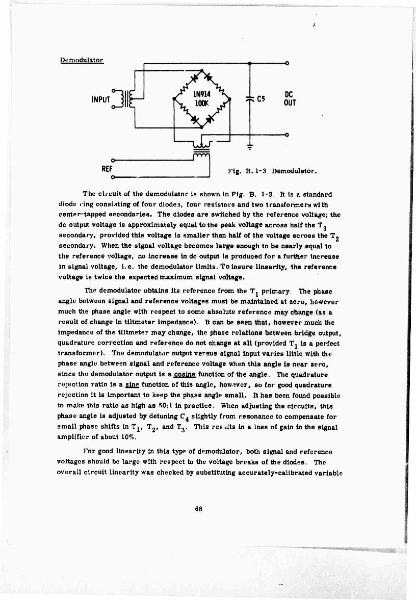
Demodulator
INPUT
Flg. B.l-3 Demodulator.
The circuit of the demodulator is shown in Fig. B. 1-3. It is a standard diode i ing consisting of four diodes, four resistors and two transformers with center-tapped secondaries. The diodes are switched by the reference voltage; the dc output voltage is approximately equal to the peak voltage across half the T„ secondary, provided this voltage is smaller than half of the voltage across the T» secondary. When the signal voltage becomes large enough to be nearly,equal to the reference voltage, no increase in dc output is produced for a further increase in signal voltage, i.e. the demodulator limits. To insure linearity, the reference voltage is twice the expected maximum signal voltage.
The demodulator obtains its reference from the T, primary. The phase angle between signal and reference voltages must be maintained at zero, however much the phase angle with respect to some absolute reference may change (as a result of change in tiltmeter impedance). It can be seen that, however much the impedance of the tiltmeter may change, the phase relations between bridge output, quadrature correction and reference do not change at all (provided T.is a perfect transformer). The demodulator output versus signal input varies little with the phase angle between signal and reference voltage when this angle Is near zero, since the demodulator output is a cosine function of the angle. The quadrature rejection ratio is a sine function of this angle, however, so for good quadrature rejection it is important to keep the phase angle small. It has been found possible to make this ratio as high as ^0:1 in practice. When adjusting the circuits, this phase angle is adjusted by detuning C4 slightly from resonance to compensate for small phase shifts in Tj, T2, and Tg. This res dts in a loss of gain in the signal amplifier of about 10%.
For good linearity in this type of demodulator, both signal and reference voltages should be large with respect to the voltage breaks of the diodes. The
overall circuit linearity was checked by substituting accurately-calibrated variable
68

air condensers for C, and C« in the tiltmeter, varying C. and C» and measuring the dc output from the demodulator. Since the nonlinearity of the system is less than 3% the linearity of the demodulator is even better.
Impedance Considerations
Common mode rejection approaching the ideal can be attained, provided the source driving the bridge (referred to Tj secondary) is at least 5000 ohms. The effect of all of the shunt paths on Tj primary (referred to the secondary) will be considered here.
XL1 JXL2 iR1 iR2 ,; Cl
C2
C2^F
-j 517.80
Fig. B. 1-4 Capacitance bridge.
All of these components are shown in the equivalent circuit in Fig. B. 1-4. An itemized list with values is shown below:
XL1' Tl shunt inductance j 56,500 ohms
XL2' T2 shunt inductance j 43,300 ohms
«1« reflected resistance from demod. 25,000 ohms
R2' reflected from quad, correction secon 156,250 ohms
CL' fixed shunting capacity (line and strays)
-j 13,200 ohms
When all of these components are added vectorially the result is:
21,550 ohms in parallel with -j 28,600 ohms
The absolute value is 17,000 ohms shunting the 30,000-ohm Z down to 10,300 ohms, still a sufficiently high input impedance for nearly-ideal linearity and common mode rejection. The most important component is seen to be R., the resistance reflected by the demodulator. This could be eliminated by interposing a buffer amplifier between T, and T« primaries, but the extra components seem to be unwarranted.
i
69
1 ■ iiiiiiii'itttflHWIliP
The effects of X. . and X. 9 are actually beneficial since they partially
tune out Cr . By placing a small adjustable inductance of the right value in parallel
with C, , it would be possible to eliminate C, entirely and make the bridge behave
as if there were no constant capacitive component. The correct value of inductance
to use in this case would be about 15 millihenrys.
70
APPENDIX B.2
SPECIAL ELECTRONICS FOR 4 MIL TILTMETER
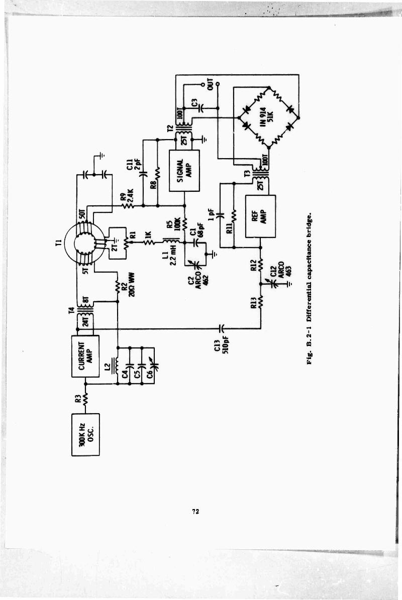
The high-frequency circuits of the 4-mil tiltmeter are shown in semi-block form in Pig. B.2-1.
Much of the circuitry has been discussed previously in Appendix B. 1, but has been modified considerably. At the risk of some repetition, it will be described again In more detail.
Overall Circuit {
The crystal oscillator drives the current amplifier; the latter's output drives bridge transformer T.. T- steps up the voltage from the current amplifier 10:1. One of its secondaries constitutes two arms of an ac bridge circuit. The other two arms consist of the differential capacity tiltmeter mercury tanks. An auxiliary winding on T via a potentiometer R^ and resonant circuit L.C.C, provides quadrature correction. The output of the bridge is the centre tap of T, 's main secondary. This signal is fed into a feedback amplifier with a voltage gain of about 28.
The output of the signal amplifier drives a phase-sensitive demodulator
which obtains its reference voltage by amplifying the voltage across T, primary with an amplifier identical to the signal amplifier. The reference voltage is applied to the demodulator via T,. The output of the demodulator is a dc signal of about 15 volts maximum which is positive for positive tilt angles, and vice versa. The dc signal is filtered by large condenser C, since speed of response is unim- portant.
Since the tiltmeter is an open-loop system, all components must have high precision and stability, and all amplifiers must employ negative feedback for both gain stability and linearity. DC drift has been reduced by making the high- frequency signal as large as possible before it is demodulated. This reduces the drift problems which may be encountered with dc amplifiers following the demodu- lator.
71
0) tu
u X) V
u
I t (4 0)
I M
n
72
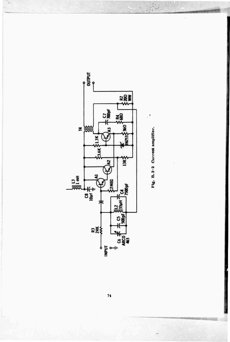
Current Amplifier
The circuit of the current amplifier is shown in Fig. B. 2-2. It consists of output stage A» operated in a common base configuration having inherently high output Impedance. A-'s low input impedance is driven by emitter follower A.. A-'s base is driven by another emitter follower A. which makes the input impedance high (100.000 ohms). Zener diode D1 holds the base of A at zero RF potential.
The output impedance at Aq's collector is about 5000 ohms. This impedance is stepped down 9:1 by T,. This is undesirable but necessary because of the low load impedance (4 ohms looking into the bridge transformer primary) which must be driven. The overall output impedance is augmented by negative current feedback
via R.. Ro. Lq» C., C5, C». The feedback factor of this network is about 2500. Feedback also increases gain stability and linearity. The parallel resonant circuit Ln« C., Cg, Cg filters the somewhat-distorted output of the crystal oscillator. The parallel resonant resistance is 2500 ohms, which together with R» and R„, determines the gain. R, C_ suppresses oscillations at extremely high frequencies. High-frequency suppression is used in several of the circuits described herein. It should be further noted that RF decoupling filters (e.g. L„ CQ) are provided in the supply leads of all circuits. The overall output impedance of the current amplifier is at least 1000 ohms. A 10% change in load resistance will produce a change in output current of 0.05%. A sourse impedance of ten times the load impedance has been found to be sufficient in practice. The current amplifier's source Impedance is at least 200 times this /alue, and therefore more than suffi- cient.
When subjected to a temperature change from 30oC to 650C, the only observable effect on the circuit was an increase in DC current drain of 1%.
Bridge Transformer
This component may be considered one of the most important parts of the system because it is a part of the tiltmeter bridge. The ferrite toroid is consid- erably larger than necessary so that all windings are in single layers minimizing inter-winding capacity. Large wire is used to reduce copper drops. Also a sufficient number of primary and secondary turns are used to produce a small magnetic flux in the core (about 400 gauss), resulting in very low core loss. Furthermore, a toriod configuration has no air gap to vary with time, temperature, clamping pressure, etc. The centre-tapped secondary forms two arms of the bridge. It is, therefore, bifilar wound so that the resistances of each half are Identical and the coupling between halves is very close. The main secondary is electrostatically shielded with copper foil on both top and bottom. Inductive reactance of the windings is so much higher (about 100 times) than the capacitive
73
I
74
reactance reflected by the tlltmeter that the transformer primary looks almost
purely capacltlve; i.e., transformer and load are operated well above their resonant frequency. A small auxiliary winding of two turns is provided for quad- rature correction. With 0.28 volt rms @ 70 mA in the primary, 2.8 volts @ 7.0 mA appears at the main secondary and 0.11 volt @ 0.44 mA at the auxiliary secondary.
A transformer is used for two of the bridge arms so that the mercury in the tiltmeter may be grounded.
Quadrature Correction
If the losses in the tiltmeter capacities are either identical or small and nearly equal, a bridge output signal of 0.314 volt rms (1 mil tilt) max exactly in phase with the primary will be produced, with a perfect null at zero tilt angle. Moreover, since the demodulator is phase-sensitive, it rejects quadrature. How- ever, some quadrature is always present, and it is bucked out by means of the two- turn winding on Tj, a potentiometer R-, and a series resonant circuit L,, C.,C2. R, is a 250-ohm wire-wound potentiometer. When C0 is adjusted for resonance, a voltage in quadrature with the bridge signal is produced. It can be made either ± quadrature because the centre tap of the two-turn secondary is grounded. The quadrature is fed into the signal amplifier via R,.. It represents only % few percent of the maximum bridge output.
Signal and Reference Amplifiers
These amplifiers are identical except for input and feedback resistors. They were designed specifically for this application because no standard amplifier could be found which had a high-enough output voltage or a large-enough open-loop gain at this frequency. It is also desirable for an amplifier of this type to recover from gross overload without "latchup", a form of hysteresis. The amplifiers require transformer-coupled outputs to drive the demodulator.
One major consideration in the design of these amplifiers was maximum output voltage (for reasons previously mentioned). It was found difficult to design output transformers with turns-ratio step-up of mor.- than 1:4 because of inter- winding capacity. However, it was possible to design amplifiers which would produce a maximum voltage of 18 volts rms at the output transformer primary (72 volts across the secondary). A second important design consideration was the maximum feedback factor. At high frequency, it is necessary to minimize the number of stages because the accumulation of phase shifts due to the input capacity of each stage leads to instability. Two stages were the most usable in this appli- cation. With only two stages, dc feedback for stabilization of the operating points became difficult. Voltage feedback was desired for low output impedance, but two
75
stages produced the wrong sense of feedback. Therefore, it was necessary to use negative current feedback. This type of feedback is desirable from all points of vU-w except for its effect on output impedance. An examination of the circuit in Fig. B.2-3 will show how these conflicting factors were handled.
DC negative current feedback via Ft. R stabilizes the operating points of A. and A . C„ is large (0.1 /if) and prevents current feedback from operating at 300 kc. It is estimated that the dc feedback factor is about 1000. AC negative voltage feedback is provided in an outer loop via a feedback winding on T,, R- and Rg. The shortcomings of this a rangement were minimized with bifilar and feed- back windings, insuring tight coupling, and taking advantage of the fact that the
loading on the output winding was a constant, high impedance. In this connection, all measurements of the amplifier output must be made either at A. collector or at the high end of the feedback winding since loading due to oscilloscope capacity will completely alter impedance relations when making measurements at the secondary terminals.
Calculation of the op«jn-loop gain of this amplifier at low frequency yields a figure of about 200,000. Due to the input capacitance of each stage, the realized gain is about 10,000. Even this value can be obtained only by making R. and R. as small as possible (limited by source impedance at the input). In spite of these limitations a feedback factor as high as 500 can be obtained, more than sufficient for the requirements.
As previously mentioned, oscillation suppression was necessary as shown in Fig. B. 2-3 by C.Q, R,0 and C^. The time constant of Rg C-- should be about 0.1 microsecond, depending upon the value of R- for the closed-loop gain required. If C-, is too small, oscillations at > ImHz will occur, while if it is too large it wil cause phase shift at the operating frequency. In any case, C,, Is very small (<10 pF).
The reference amplifier (B.2 4) is operated at a voltage gain two-three times
higher than the signal amplifier. Consequently, its feedback factor and performance are correspondingly lower. However, the requirements of the reference amplifier are lower. The only difference between these amplifiers is in input circuitry. The signal amplifier contains provision for two inputs: bridge and quadrature correction, while the reference amplifier has provision for a precise adjustment of the phase angle between signal and reference voltages. A summary of signal amplifier performance is given below:
76

SIG.IN
QUAD.IN
25yf ^
0.002Mf /ok
o OUTPUT
C' * 1560 0.1 pf
2mH
RIO lOOfi
-15V DC
Fig. B.2-3 Signal amplifier.
77
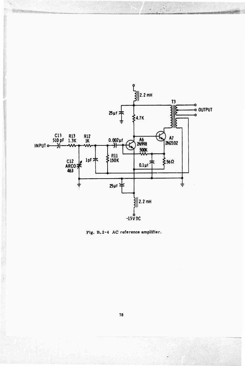
o OUTPUT
C13 R13 R12 510pF 1.3K IK 0.002Mf ^
INPUTo—)|—vvAr-f-^/w-^ T yl T^UJ
-15V nc
Fig. B.2-4 AC reference amplifier,
78

Feedback factor:
Output impedance:
Harmonic distortion:
Overload point:
Input impedance:
Noise;
500
15 ohms
0. 15%
14. 7 volts rms
2.4K
0. 7 mv rms
Tests for Putting System into Operation
Equipment required
Oscilloscope with zero phase shift in X and Y inputs at 300 kc and capable
of detecting 0. 5 mV at Y input at dc and 300 kc. If the tiltmeter itself is not
available, it may be simulated by fixed condensers and trimmers. To simulate
null, each condenser should have about 2250 pF capacity. To simulate maximum tilt, one should have 1850, the other 2917 pF.
Step 1
Scope X at output of crystal oscillator; scope Y at high end of R™ (20-ohm
resistor in current amplifier); adjust C6 until voltage across R, peaks. It should
peak at 1.4 volts rms approximately in phase with the input. If this voltage is not
this value, change Rg. Transfer scope Y to high end of Tj primary. The voltage there should be 0. 28 volts in quadrature with the input.
Step 2
Scope X at high end of T- primary; scope Y at high end of signal amplifier
(TJ feedback winding; make simulated tiltmeter condensers 2250 pF each (adjust
for null). Set R- at one end of its travel and adjust C„ for open ellipse or circle.
Y should have maximum amplitude for this setting of C?.
Step 3
Make one simulated tiltmeter condenser 1850 pF; the other 2917 pF (maxi-
mum tilt); the voltage at the signal amplifier feedback winding should be between
8 and 9 volts rms. It may be adjusted by changing the value of R_.
Step 4
Scope Y at high end T. primary; scope X at high end of feedback winding of
the reference amplifier; the voltage at this point should be between 12 and 14 volts
rms. It may be adjusted by changing the value of R,,.
79

Step 5
Scope X at high end of T. primary; scope Y at demod output; scope set for dc; simulated tiltmeter capacity as in Step 3; demodulator dc output should be about 15 volts; reversing the positions of 1850 pF and 2917 pF condensers should produce the same demodulator output with reversed polarity (the two polarities will
differ somewhat if there is appreciable demodulator unbalance at bridge null).
Step 6
Scope as in Step 5; simulated tiltmeter capacity as in Step 2. Turn R, through its full travel and adjust C*, so that changing R. does not change demodu- lator output (this puts signal and reference voltages exactly in phase for best quadrature rejection). C., should be selected by trial so that Cj, Is near the middle of its range when quadrature rejection is obtained. If C.« must be made Lsrger for quadrature rejection, C., should be made larger, and vice versa. After these adjustments have been made, check the reference voltage again as in Step 4.
Step 7
Scope X at high end of T. primary; scope Y at high end of signal amplifier feedback winding; simulated tiltmeter condensers 2250 pF each; adjust these and R- for null (a few millivolts).
80

APPENDIX B.3
OPERATION OF DIODE RING DEMODULATOR
The circuit of the diode ring demodulator is shown in Fig. B. 3-1 (a). The reference voltage must be larger than the signal voltage. Suppose that, at some instant, point A is positive with respect to point B; diodes D. and D» conduct and the circuit can be redrawn as in Fig. B.3-1 (b). Since Dg and D, are reverse-biased by the reference voltage at this instant, they can be considered open circuit. The whole reference secondary is charged to 1/2 the signal secondary potential through R. and R»» as is C.
On the next half-cycle, the conditions are shown in Fig. B. 3-1 (c). D, and D, conduct, while D. and D- are open circuits. The circuit behaves exactly as on the first half-cycle, except C is charged through R? and R, instead of R. and R,- C is still charged positively, since the upper half of the signal secondary is positive on this half-cycle.
Thus it is seen that the rectification is full wave and that C is charged to 1/2 the peak voltage of the reference secondary, provided R. and R. (and R„ and RJ in parallel constitute with C a short time-constant compared with half an ac period, and RC is long. This implies that the resistors should be made as small as possible (provided the reference and signal sources can supply the current), and that the diodes1 forward impedance should be low. Also, C should be loaded as lightly as possible (R large). Therefore, the diode ring demodulator has a low- input impedance and a high-output impedance.
There is amplitude comparison between the instantaneous potential on C and the signal potential, since the diodes are held switched on by the reference voltage, and signal current can flow through them in either direction. Therefore the output of the demodulator is updated with respect to the signal on each half- cycle. This property is important when speed of response must be considered.
If the signal secondary terminals were reversed with respect to the refer- ence secondaries (or vice versa), the charge on C would be reversed also. There- fore, the rectification is phase-sensitive.
81
p
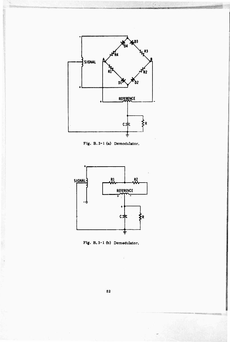
. >•
Fig. B.3-1 (a) Demodulator.
IGNAL i I WV *■
R2
REFERENCE
+ t
C*
Flg. B.3-1 (b) Demodulator.
82
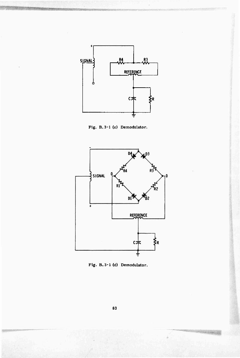
5 CNALj R4 R3 I—wv——i—vw-
REFERENCE
n Fig. B. 3-1 (c) Demodulator.
Fig. B.3-1 (d) Demodulator.
83

If the signal voltage is in quadrature with the reference (or contains a quadrature component), a signal voltage will be present while the reference voltage is passing through zero. Under these condidons, the diodes will be switched by the signal voltage only, as in Fig. B.3-4. Diodes D- and D, will conduct, while Dj and D, will be open. The voltage at the junction of R, and R» will be the same as at the signal secondary center tap, and there will be no potential difference to charge C. On the opposite half-cycle the action is the same, except that D. and D. conduct while D9 and D» are open. Thus, the quadrature component gives zero output, i.e., the diode ring demodulator rejects quadrature.
If there is no reference voltage present, there will be no demodulator output provided the circuit is perfectly balanced. This action will also take place if the reference voltage is smaller than the signal voltage. In fact, the demodu- lator output will be approximately equal to one-half the signal secondary peak voltage until the latter approaches the reference value. If the signal voltage is made larger than the reference voltage, there will be no further increase in demodulator output, i.e., the demodulator limits.
84

APPENDK B.4
CERTAIN NONLINEARITIES AND ERRORS IN A CAPACITIVE BRIDGE TILTMETER
The electrical arrangement for the capacitive bridge tiltmeter is shown in Fig. B.4-1.
0 WA>—i
TRANSMISSION LINE
^1
MERCURY
xxxx\\\\\\\\\\\\x\\\\\\\\\v
Fig. B.4-1 Capacitance bridge tiltmeter.
Linearity and Scale Factor
If each gap were 40 mils at zero tilt and K = 5 for the oil in the gap, Cj = (8000/tj) + 50 pF and C, ■ (8000/t,) + 50 pF where tj is the thickness of gap 1 and t« is the thickness of gap 2. The extra 50 pF in each equation is the capacity of each transmission line and strays.
If we redraw Fig. B. 4-1 schematically we have:
m
EIN
I 1 I
C2
T E0UT
Fig. B. 4-2 Bridge transformer.
85

For a 1:1 ratio center-tapped transformer,
Ej>ut . i . 5fl B 4 . E in 2 Xcj + Xc2 *'*'*
Bout _ 1 u>cl mA9 EüT ' 2 1 , 1 B42
or
OJC. U)C9
E out - 1 C2 E in 2 Cj + C2
B*-,J
If we assume that all of the capacity is variable (i.e., neglect the trans- mission lines and strays)
and
Substituting (4) and (3) in (3)
cl ■ 8000
H
C2 = 8000
in (3)
8000
E out i h . 1 2
h E in " 2 8000 + 8000 H*h
B.4.4
B.4.5
B.4.6
for gaps of 40 mil varying i 1 mil
|-^ = -j - 394
4.141 = 0.0125 volt/mil tilt/volt bridge excitation.
Since 10 mil tilt gives exactly 10 times the output as 1 mil, the linearity is perfect.
If we make the gaps 4 mil ± 1 mil max, we obtain exactly the same result.
Since the constant part of the capacity cannot be neglected in practice, we substitute Eq (B.4.1) and (B.4.2) into (B.4.3) to take this component into account:
since tj + t2 = 80 mils, t2 = 80 - tj and
86

8000
E out __ E in ' 8000
80-t, + 50
80-t, + 50 + IfiOO + ^
or
E out ± E in ' 2 '
240t - t'
12,800 + I60t - 2t' B 4.7
It can be seen from Eq (B. 4. 7) that the fixed component cf capacity introduces higher-order terms which affect the linearity.
To determine the magnitude of this effect, let t= 41 mil; from Eq (B. 4. 7)
ff1 s T " 12.80^ "SSM-3362 = 0 01000 volt/mil lüt/VjiS2S
The first result of adding the line capacity is seen to be a reduction in bridge sensi- tivity of 25%
if we let tj = 50 (10 mil of tilt)
E out ,. 1 12.000 - 2.500 . n ln1,RR Ein "2 12,800 + 8003 - 5000 w-1"1"»
The second result of adding the line capacity is the introduction of a 1. 266% nonlinearity at maximum tilt. It can be shown that this nonlinearity is a smaller percentage for smaller tilt angle.
If we make the gaps 4 mil ± 1 mil, Eq (B 4. 7) becomes
E out „ _1_ E in ~ 2
168t - t" 1280 + 16t - 2t
B 4.8
Let tj = 4.1 mil
E out _ E in " 1286088+65"66-33.6 = 0. 012195 volts/0. 1 mil/volt
Let t. = 5 mil
E out _ Tin" " JM ' 0
25_ . =0.012214 volt/0. 1 mil/volt 1280 +80-50
87
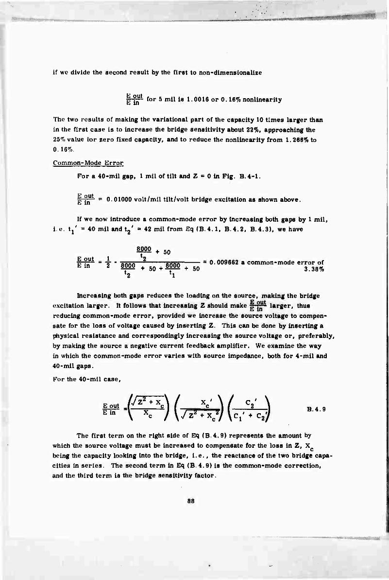
if we divide the second result by the first to non-dimensionalize
|-gp for 5 mil is 1.0016 or 0.16% nonlinearlty
The two results of making the variational part of the capacity 10 times larger than in the first case is to increase the bridge sensitivity about 22%, approaching the 25% value tor zero fixed capacity, and to reduce the nonllnearity from 1. 266% to 0. 16%
Common-Mode Error
For a 40-miI gap, 1 mil of tilt and Z = 0 in Fig. B. 4-1.
| °rc = 0.01000 volt/mil tilt/volt bridge excitation as shown above.
If we now introduce a common-mode error by increasing both gaps by 1 mil, i.e. tj' = 40 mil and t2' ■ 42 mil from Eq (B.4.1, B.4.2, B.4.3), we have
5500+50 E out 1 2 TT-J— ■ T * nnnn— önnn " 0 009662 a common-mode error of Ein 2 SJOO + 50 + SJOO + 50 3 38%
H h
Increasing both gaps reduces the loading on the source, making the bridge excitation larger. It follows that increasing Z should make „ ?" larger, thus reducing common-mode error, provided we increase the source voltage to compen- sate for the loss of voltage caused by inserting Z. This can be done by inserting a physical resistance and correspondingly increasing the source voltage or, preferably, by making the source a negative current feedback amplifier. We examine the way in which the common-mode error varies with source impedance, both for 4-mil and 40-mil gaps.
For the 40-mil case.
{-^V \77T^j \^j |_^t ^ _ . j l ^„^^^j I " I B.4.9
The first term on the right side of Eq (B.4.9) represents the amount by which the source voltage must be increased to compensate for the loss in Z, X being the capacity looking into the bridge, i.e., the reactance of the two bridge capa- cities in series. The second term in Eq (B.4.9) is the common-mode correction, and the third term is the bridge sensitivity factor.
88

X and X,.' are found by X^ = - , *, C C ' 6 3 w 18
for f ■ 300kc
X ■ 4246 ohms and X ' = 4329 ohms c c
C '
C ' ^2
250.OpF
240.5pF
255,IpF
245.IpF
Substituting these values in Eq (B. 4.9) we obtain
Eout _ fJz2 + 4246Z \ / 4329 \ E in "^ 4246 j ^ + 43292y (0.009662)
^ P" is the bridge output with common mode error. We wish to vary Z to see what effect it has on that error. If first we make Z very large, we see that the
4329 CM error approaches a limit-r-Tg x 10338 = 0.009851, a common-mode error of 1.49%. This shows that, with a perfect current source (infinite Z), the CM error is still nearly half of the uncorrected value. This is because the line capacity
4 shunts and therefore limits the source impedance Z. If we make Z = 10 , the common mode error is 1. 55%, or near enough to the limit for all practical purposes. In this case, a source impedance of 2 to 3 times the bridge impedance is the maximum useiul value.
For the 4-mil gap we substitute values in Eq (B. 4.9) as before and obtain
out _ I Jz* + 571.8Mf 528.3 \ in \ 5i78 lyj + Koj) (0.01188)
For Z = 0 (uncompensated for CM),
ll^ = 0.01188 volts/0. 1 mil/volt bridge excitation
This represents a CM error of 2. 58%. For large Z, the CM error approaches a limit of
s|!j g x 0.01188 = 0.012121 = 0.61%
For a Z for 5000 ohms the CM error is 0. 66%, near enough to the limit for all practical purposes. In this case a source impedance of about ten times the bridge
89

impedance is the maximum useful value. It is higher than in the former case because of the reduced shunting by the fixed capacity.
Conclusion
A large fixed value shunting the variable cj.pacitive component is detrimental in three ways:
1. It reduces bridge sensitivity.
2. It increases bridge nonlinearity.
3. It makes it impossible to improve common-mode rejection appreciably by increasing the source impedance above a certain value.
One minor factor which has not been considered is the variation of bridge impedance with tilt angle. In this respect, a fixed capacitive component is helpful, but this factor is too small to be of significance.
It has been demonstrated that increasing the bridge capacity (decreasing the gap) is beneficial in three ways. It has been found possible to increase the bridge excitation 50% and drive impedance to 5000 ohms with a drive amplifier of reliable design. A 4-mil gap increases the sensitivity by 1220%.
90

■'v,"/'
APPENDIX B. 5
STUDY OF LINEARITY VERSUS CAPACITOR GAP
91
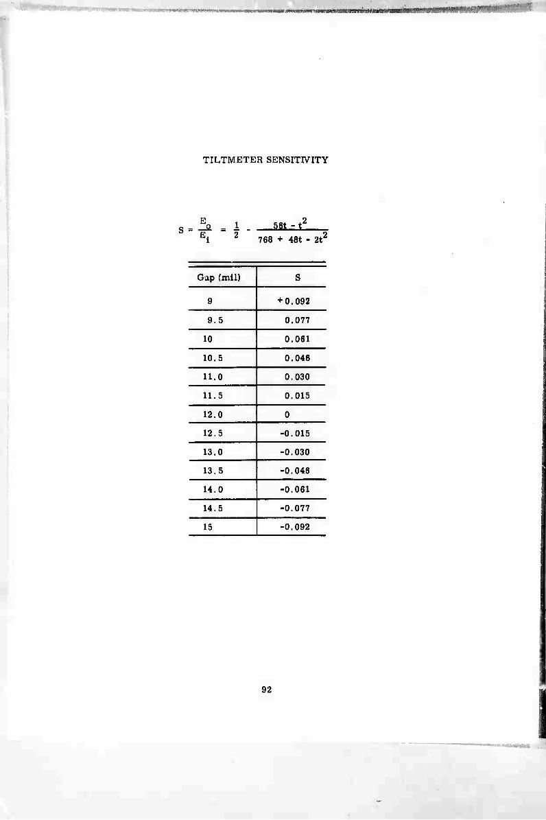
■ ■ ■■■;..■•, ■
TILTMETER SENSITIVITY
E 3'<
56t - t^
768 + 48t - 2t'
Gap (mil) S
9 + 0.092
9.5 0.077
10 0.061
10.5 0.046
11.0 0.030
11.5 0.015
12.0 0
12.5 -0.015
13.0 -0.030
13.5 -0.046
14.0 -0.061
14.5 -0.077
15 -0.092
92

I
£ CM
I to 3 (0
s i
I E PQ
(0 t
o «.
93
■mem— nW.IIIKB i ■ mm~mmmm&*immmim
It
1
;U rf«—
' ■ 1 'MfeMMitt^} "
.
lAwMiiiriiiiilajtiai^^^^^
-
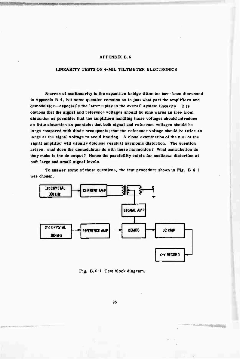
APPENDIX B.6
LINEARITY TESTS ON 4-MIL TILTMETER ELECTRONICS
Sources of nonlinearlty in the capacitive bridge tiltmeter have been discussed in Appendix B.4, but some question remains as to just what part the amplifiers and demodulator—especially the latter—play in the overall system linearity. It is obvious that the signal and reference voltages should be sine waves as free from distortion as possible; that the amplifiers handling these voltages should introduce as little distortion as possible; that both signal and reference voltages should be large compared with diode breakpoints; that the reference voltage should be twice as large as the signal voltage to avoid limiting. A close examination of the null of the signal amplifier will usually disclose residual harmonic distortion. The question arises, what does the demodulator do with these harmonics? What contribution do they make to the do output ? Hence the possibility exists for nonlinear distortion at both large and small signal levels.
To answer some of these questions, the test procedure shown in Pig. B. 6-1 was chosen.
li\ CRYSTAL 300 kHz
— CURRENT AMP 4 ■ b ^
R
SIGNA! AMP
1 2nd CRYSTAL
300 kHz -* REFERENCE AMP —* DEMOD DC AMP
X-Y RECORD -J
Fig. B.6-1 Test block diagram.
95

The idea behind this scheme was that when a phase-sensitive demodulator is driven from two independent ac sources, the output of the demodulator, instead of being dc, is a low frequency ac beat corresponding to the frequency difference between the two sources. For this beat to be purely sinusoidal, every component in the system must be linear.
Exactly the same components used in the tiltmeter were used in this test, the only differences being that the reference amplifier was driven from a second crystal oscillator, and the capacitive bridge was replaced by the potentiometer R for greater convenience in setting the signal amplifier input. The linearity was tested over four decades of signal amplifier input (simulated tilt angle). The chosen amplitudes and gains are shown in the table below:
Tilt angle Input to sig amp Demod output DC amp gain DC amp out
± 1.0 mil 314 00 mv rma 30000 Vpp 1/30 IVpp
± 0. 1 mil 31.40mv rma 3.000 Vpp 1/3 IVpp
±10M inch 3.14 mv rma 0.300 Vpp 10/3 IVpp
± Ifi inch 314. 00M V rms 0.030 Vpp 100/3 IVpp
± 0. 1 M inch 31.40MV rms 0.003 Vpp 1000/3 IVpp
The dc amplifier used was a high-precision, very low drift type with an open-loop voltage gain of 10 . Thus, in Its maximum gain position it still had a feedback factor of over 3000. It was always operated at the same output, and the amplitude was always 1 volt peak-to-peak (5% of its maximum dynamic range). It was therefore unlikely that this amplifier contributed significant distortion to the data.
It was convenient to display the data on paper as a permanent record. For this purpose, an X-Y recorder was used, having a 10-inch vertical scale and a 15-inch horizontal scale. The data could be "blown up" to a rather large value for close examination.
Since the X-Y recorder slewing speed was limited, the beat frequency had to be very low, i.e., only a fraction of one Hz The oscillators were provided with frequency verniers, a great convenience in adjusting the beat frequency.
The beat frequency was fed into the Y axis of the recorder, while the X signal was provided by a linear sweep built into the recorder When a record was nade, the beat frequency and the X sweep speed were so adjusted that three zero
crossings were displayed so that any change in either beat frequency or sweep speed could be seen by measuring the intervals between zero crossings. No diffi- culty was experienced from this source.
The linearity was checked by comparing ordinates drawn by the recorder with ordinates taken from a trigonometric table. These points were taken every 20° and are shown by dots. Over ths first three decades (Fig. B. 6-2a, b, c, and d) the linearity was as close as one could measure (1% or better). In the fourth (Fig. B.6-2e) decade the data were largely masked by noise. This difficulty was not unexpected because of the unnecessarily large system bandwidth ( 200 Hs) and the extremely small signal amplitude. With a filter placed between the dc amplifier and recorder to reduce the bandwidth to a few Hz, meaningful uata could be obtained, and it could be seen that considerable distortion did indeed exist (as much as 10%). It could also be seen that the quadrature bucking circuit had an appreciable effect on the distor- tion and that reducing the beat frequency increased the distortion. In this type of test the presence of any quadrature at all would contribute to distortion because, with a continuously rotating phase angle between signal and reference, the quadrature would add to the demodulator output for one phase angle, subtract from it for another phase angle, and contribute nothing at other phase angles. Introducing the low-pass filter made the distortion seem less, except at low beat frequencies, because it suppressed the distortion as well as the noise. In other words this test fails where appreciable quadrature exists. Such distortion is probably not present under work- ing conditions. However, the quadrature component is so small that the test was valid down to a simulated displacement of less than 1 microinch and inconclusive for smaller displacements. With very careful quadrature adjustment an undistorted curve for this decade was obtained.
A test more representative of working conditions would be to feed into the signal amplifier a suppressed 300 kHz carrier modulated by a low-frequency oscil- lator, and record the demodulator output as before. The problem with this arrangement is the difficulty of generating a suppressed carrier with sufficient linearity; in other words, the instrument under test is so good that it is difficult to find a sufficient test method.
♦ See Fig. B.6-2 (f).
97
■

0 20 40 60 80 100 120 140 160
200 220 240 260 280 300 320 340
Fig. B.6-2 (a) Bridge output.
98

Fig. B.6-2 (b) Bridge output.
99

Fig. B.6-2 (c) Bridge output.
100
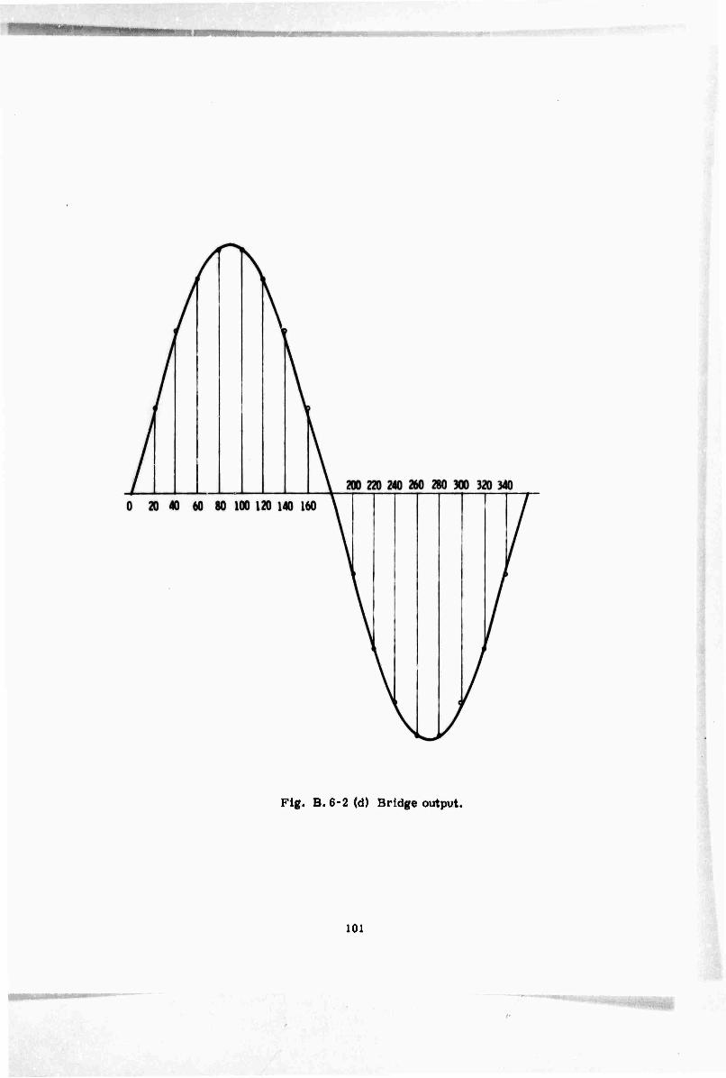
Fig. B.6-2(d) Bridge output.
101
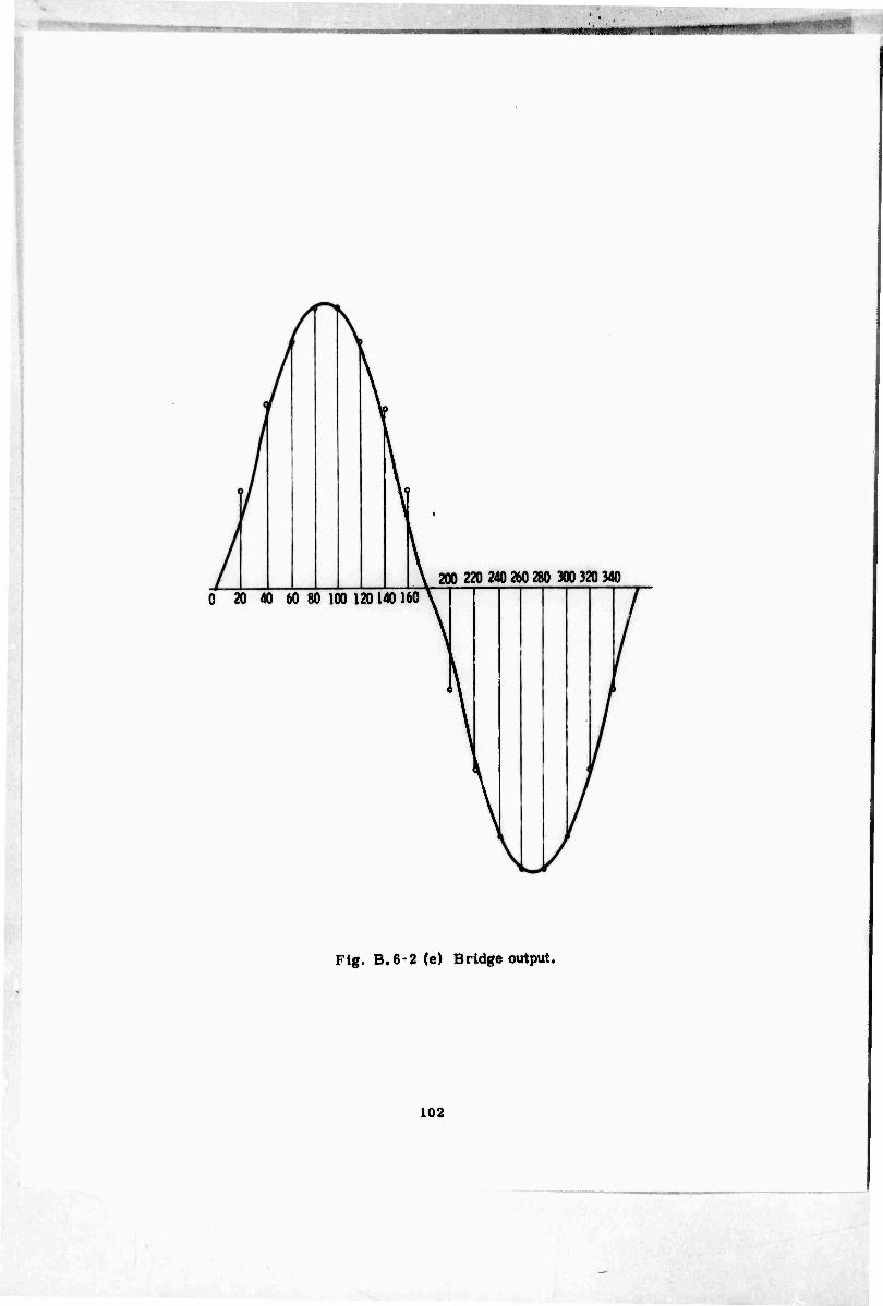
-♦- - , J ,.,„,„■»/.-
200 220 240 260 280 300 320 340 0 20 40 60 80 100 120 140 160
Flg. B.6-2 (e) Bridge output.

Flg. B. 6-2 (f) Bridge output.
103

■■f,a.mm^nmmmim0!0mmmfmi0tM
MOKC CRYSTAL
OSCIUATOR
CURRENT AMPLIFIER
RINC RESONANT FILTER MODULATOR
LF FUNCTION GENERATOR
r
REFERENCE AMPLIFIER
DEMOO SIGNAL
AMPLIFIER
I
4_ i i
I i L SYSTEM UNDER TEST
i
i j
em linearity test diagram. X■Y RECORDER
Since the first test described above indicated that the linearity of the ring
demodulator was very good, it was thought probable that the identical circuit used
as a modulator would have good enough linearity to test the system. Therefore, the
second procedure as shown in Fig. B. 6-3 was chosen.
The diode ring modulator generates a 300 KC suppressed carrier, while a
function generator provides the envelope. Since the modulator carrier output wave-
form is a square wave, it was filtered by a resonant LC circuit, tuned to 300 KC.
Filtering was necessary because the limited system bandwidth might distort the
square wave and contribute to errors. The wave shape of the function generator was
a symmetrical ramp. The linearity of this ramp waveform was 0. l%or better. The
advantage of using a ramp instead of a sine wave is that the linearity can be inspected directly so that use of trigonometry tables is unnecessary.
The results of the second test are shown in Fig. B.6-4a, b, c, d and e. It can be seen in Flg. B. 6-4 that ther« is some demod limiting present, amounting
to symmetrical distortion of about 3%. In this case the signal amplitude is about
half that of the reference. If the signal were made larger without increasing the
reference amplitude, this distortion would increase rapidly. This distortion is so
small in Fig. B. 6-4b< c and d that it cannot be measured (probably less than 0. 5%).
In Fig. B. 6-4e the signal is so small that the noise is the limiting factor but the dis- tortion is still less than 1%. Visual inspection of this smallest amplitude on the
cathode ray oscilloscope shows lower distortion than the X-Y recorder displays. It
is difficult to obtain a very good plot on the X-Y recorder at such low amplitudes be-
cause of system drifts during the recording time.
The purpose of the system under test is to provide a voltage proportional to
tilt angle at very low seismic frequencies i> 1 Hz), For applications where greater
speeds are required the bandwidth capability of the electronics is 350 Hz for a reso-
of 4 nanoinches. This bandwidth is obtained when sufficient filtering is used to re-
duce the demod ripple to white noise level.
104
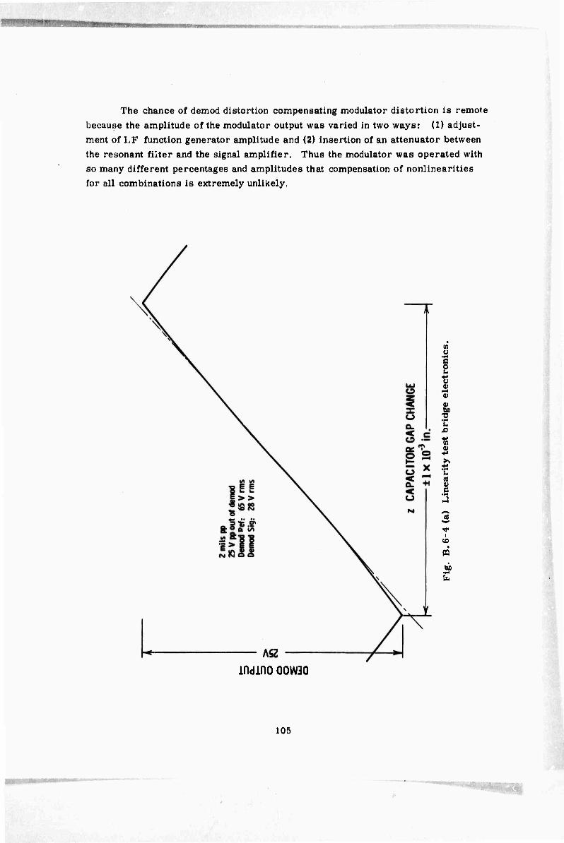
The chance of demod distortion compensating modulator distortion is remote
because the amplitude of the modulator output was varied in two ways: (1) adjust-
ment of LF function generator amplitude and (2) insertion of an attenuator between
the resonant filter and the signal amplifier. Thus the modulator was operated with
so many different percentages and amplitudes that compensation of nonlinearities for all combinations is extremely unlikely.
(A a
•i^
s o u +» Ü 0)
0) bo "0 h
i)
u
i CD
m
•M
indino Q0IAI3Q
105
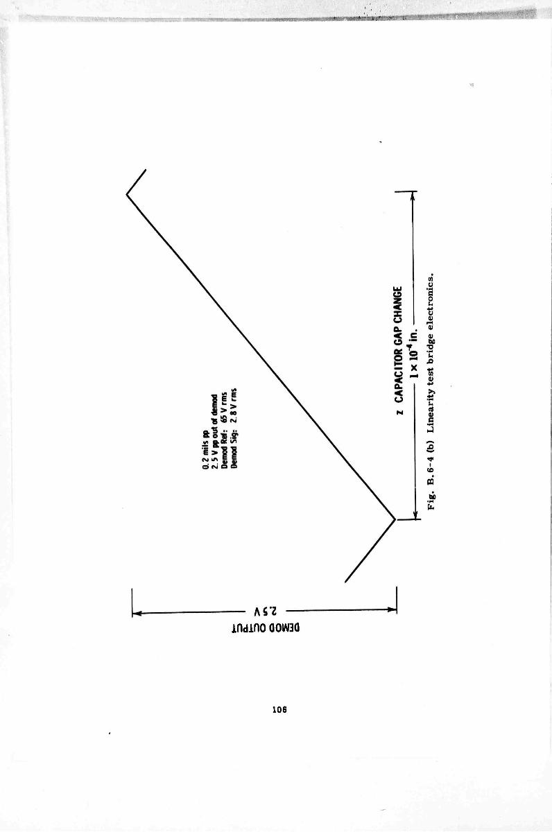
indino QOW3G
106

ü
4)
0) be
u XI
01
rt
I
I
pa
u
i/ldinO G0W3Q
107

ü •ft
I
So T3
I
(I) i 3
I to
PQ
tuo
indino QOIAI3Q
108

c o u f 0)
01
y 'C ■a
0)
I CD
be
IfldinO Q0W3Q
109


APPENDIX B.7
CIRCUIT DIAGRAMS
111
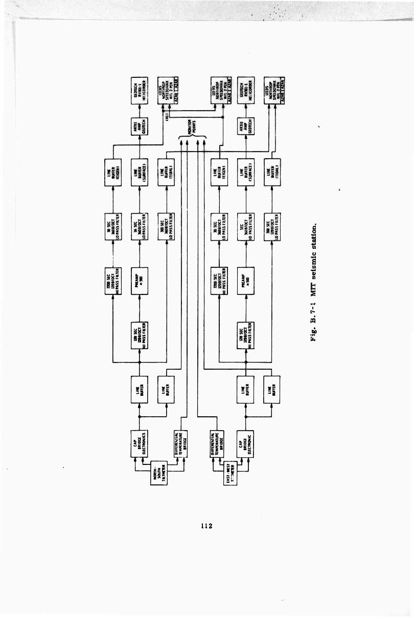
112

i
113

a) be •o
•r-t U Si u 01
I CO
i
i
114
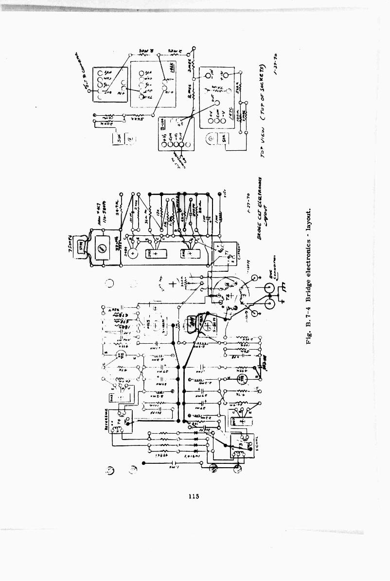
2 t
1) be •o
i
n
115

. ,
HI PASS 7200 SEC
12 OB/OCT
INPUT O- 75M' 2.2MEG 75M' h
34 M' 2.2MEG -vw—i
36MEG 7.2MEG 36MEG
23ur-p -y- 23Mf
2uf 2Mf
LO PASS 30 SEC
360B/OCT
S0.5MEG
i—vW 1(—i
2MEG 4MEG 2MEG '
«Oi
2Mf ^2Mf
4MEG 4MEG I-VW-|-/W-I
:iMf
-8 MEG
2Mf 2Mf
H(-r-H(- |0.5MEG|
4MEGi O-'M' f-vw^—It—
4MEG 4MEG
OUTPUT
Fig. B.7-5 Eigen filter.
116
.
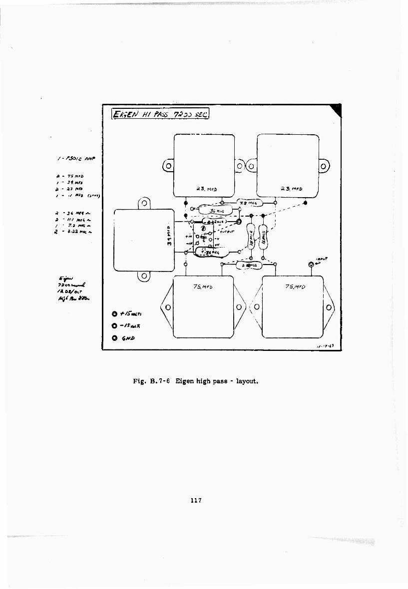
/ - /150/c Amf
a - 7sn'D
Z - >•& UK *
\EfcCrf /// /^ 7^^ ^C.
(° OKO °)
,/.//•<>
Fig. B.7-6 Eigen high pass - layout.
117
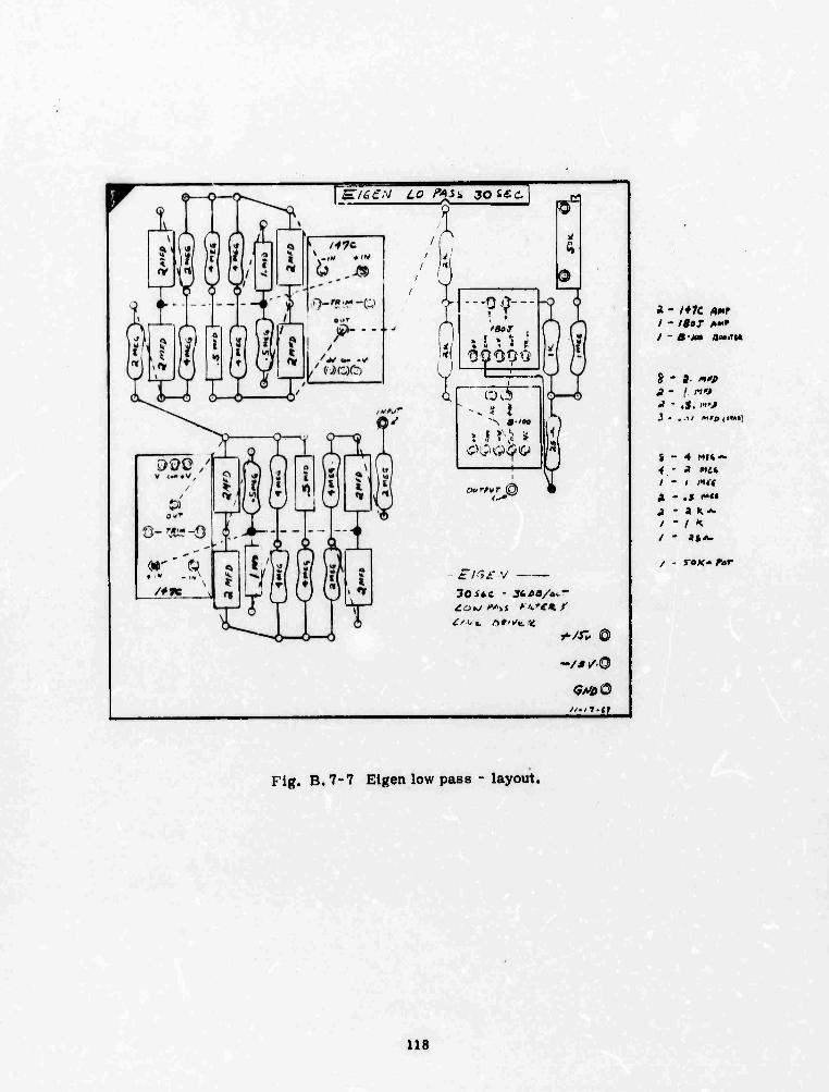
1 I i*^m>^^*m~^~-~*
^^P25 1 w / /'«
(«r ®
A -o.'?---
/flay
" D3
Sl<%£N Jostc -
C'\ c. .^If i/i«
//■'T.«>
a - UK. A*r
y - a. /•«)
n - .S. n'i
S - 4 Mf«-«- < - ^ IH£« / - / /It"*
^ - a K-«- / - / ** / - as-o-
/ - 5-OAC-« Far
Fig. B. 7-7 Eigen low pass - layout.
118
.._^^«MUi MiBaaaMMHMMIMMMMM
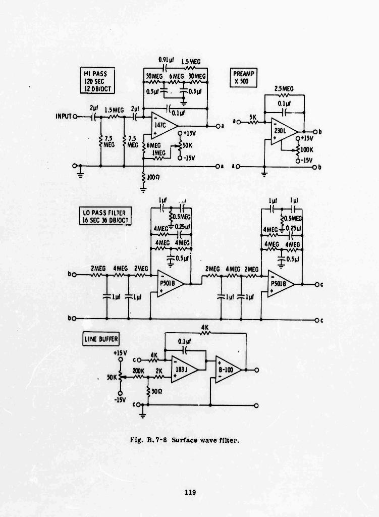
mm —- I n i i mm MM im
HI PASS 120 SEC 12 0B/OCT
2M' 1.5MEG 2Mf k
INPUT O 1 (-w^-^_) f-i-
7.5
^fM» 1.5MEC —^f VVA^—i
30MEG 6MEG 30MEG
0.5u'-r -T« 0.5 jil
4—Oa
MEG ?MEC iöMEG rKMK
n AV—I i-15V
T-* SlOOfi
-Oa ao
LO PASS FILTER 16 SEC 36 DB/OCT
lM» -J H(-H(-
$0.5MEG
4MEG^01-25M'
2MEG 4MEG 2MEG
4MEG 4MEG
^0.5Mf
?0.5MEG
4MEGi-0;?5"' f-vVA—Hf-
lUf IM' HHHf-
4MEG 4MEG
:0.5M'
Flg. B.7-8 Surface wave filter.
119
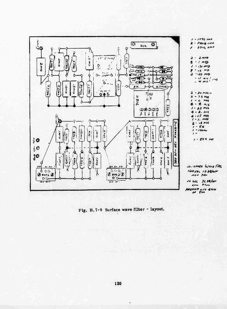
wmmmiim m*m
/ - /*7C /»•'
J - ifV'P
/ - •?/ /*'0 f - ,* *<» J -OS /»»Ö
- ./ *.* ? I
J - 7.5 rtr^ / - *. »«5 0 - # «.« / - j,r A.«
4 - *• A«? A . /.r «/« / - /. /««« 2 ■ .s i»r< / - «■«
/ - /eo-n.
•i»
/ -
r«« wr
ftia M /Mi
Q4 r»»
Fig. B.7-9 Surface wave filter - layout.
120

i ^mm—mmm
1
1 # # # # 1 4
« 1 Ü V i «
i r
k ^♦<5SD-r —oo 1
Jc So< 'S H
1 i '♦ * S r- U ^ it»/ \» i
V L r I
8
/1
1 |
*J 1
i. l 'Q
' \o (
n 1 n\ 1 «I j> ^ ! \ ^ 1
w 1 fv 1 \ 1
^. i ■ k\ ^ 1 t»l I • $1 b ''■ V 1
1 f ^ 1 f»| o^ S » ",
1; V
R' i "
d ̂
/ - •/ if't
J ■ t K
/ - »-»A.
Flg. B. 7-10 Surface wave filter - line driver.
121
■HMMHlMMHM^HMi^HiM ■ li 11 i — i i
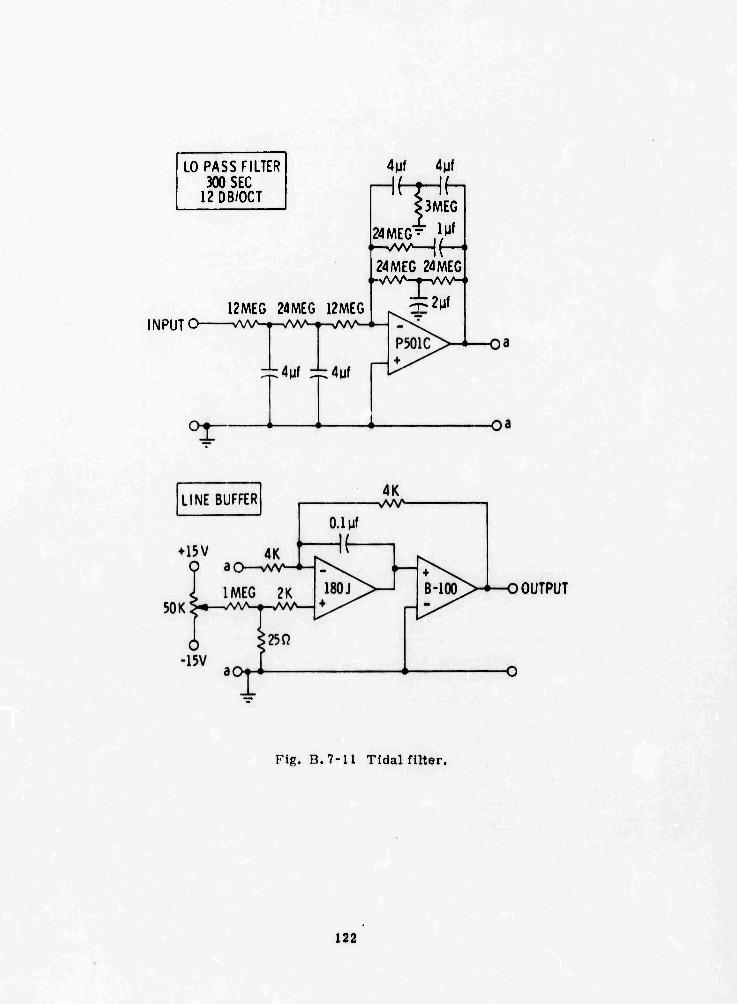
'' ll1 vmmmmmmmmim^mim ■ HUI
LO PASS FILTER 300 SEC
12 DB/OCT
4uf 4Mf
Hf-f
INPUT O- 12MEG 24IV\EG 12MEG
^3MEG
24MEG" W
24MEG 24MEG | »->A/VV—»-VW-•
iiiif
OUTPUT
Fig. B.7-11 Tidal filter.
122
'■—*»■**—-■■ ■■-■— - —iBM^MMi^t^

1 " ' 1 ' <
ntbAi. jfrjn je C IJbB/a^ i.J«/ /Vilj i-l.Tft (
- '*« »« :,', *'S*®
-/U'®
G*»Q
ULUi
/ - Prai c jn»r /-/9oT **>» / -0-1 a» tmutm
■f-'f »»A
/ - / /*'*
/ - 3 riff / - / »«j 4 • f «* / - A /< / - JJ ■"•
/ - SOX. PaT
rig. B.7-12 Tidal filter- layout.
123
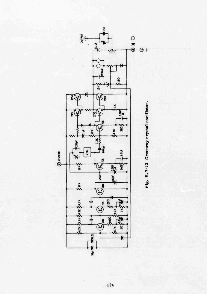
i imii^^^mmmmmmmmmm M^^^^Vn,
rtaMMMMtMH •-- •■' - •■■ ■:,:' "' " '
JL—t-© e-+
u o
u (0 o 1
g c V fa Ü
I t-
byo
124
- ■ —

—._ ..•-.—--'—. .
mmmmmmmm r..>:..-.: ■ , -.
O NAV-Vi/V-A/\A^ O
• I »« I
S
I
3
i a
125
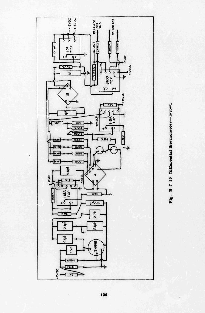
, __
V
V
1 t
m I
n'
fa
126
n —a■