QSAR and 3D QSAR in drug design Part 1: methodology Hugo Kubinyi

Classical QSAR methods describe structure-activity

relationships in terms of physicochemical parameters

and steric properties (Hansch analysis, extrathermo-

dynamic approach), or certain structural features (Free

Wilson analysis). 3D QSAR methods, especially

comparative molecular field analysis, consider the three-

dimensional structures and the binding modes of protein

ligands. Quantitative similarity-activity relationships

derive correlations between the similarities of individual

compounds and their biological activities. Theory and

methodology of these approaches are described here,

together with the proper use of regression and partial

least squares analyses for deriving quantitative structure-

activity relationships. Part 2, to be published in the

December issue, will address applications and problems.

Q uantitative structure-activity relationships

(QSAR) correlate, within congeneric series of

compounds, affinities of ligands to their binding

sites, inhibition constants, rate constants, and

other biological activities, either with certain structural

features (Free Wilson analysis) or with atomic, group or

molecular properties, such as lipophilicity, polarizability,

electronic and steric properties (Han;sch analysis) 1-13.

Although relationships between lipophilicity and unspecific

biological properties, such as narcotic, bactericidal, fungici-

dal, hemolytic and toxic properties, have been known since

the turn of our century, the independent publications of the

Free Wilson method 14 and of Hansch analysis 15, both in

1964, mark a milestone in the development of QSAR.

Since then, QSAR equations have been used to describe

thousands of biological activities within different series of

drugs and drug candidates. Especially enzyme inhibition

data have been successfully correlated with physicochemi-

cal properties of the ligands 1-3,16. In cen:ain cases, where

X-ray structures of the proteins became available, the results

of QSAR regression models could be interpreted with the

additional information from the three-climensional (31))

structures~-3.

After a very slow development of grid-based 3D QSAR

approaches, in 1988 the method of comparative molecular

field analysis (CoMFA) was published by Cramer et al. 17

This molecular field-based method constituted the first real

3D QSAR method. In the past ten years, many successful

CoMFA applications proved the value of this method 1~--'4,

especially in cases where classical QSAR methods fail. In

contrast to Hansch or Free Wilson analysis, CoMFA is better

suited to describe ligand-receptor interactions, because it

considers the properties of the ligands in their (supposed)

bioactive conformations. As the result of a CoMFA analysis,

regions in space are identified that are favorable or unfavor-

able for the ligand-receptor interaction.

Hugo Kubinyi, Drug Design, ZHV/W-A30, BASF AG, D-67056 Ludwigshafen, Germany. tel: +49 621 60 42115, fax: +49 621 60 20914, e-mail: kubinyi@zhv.basf-ag.de

DDT Vol. 2, No. 11 November 1997 Copyright © Elsevier Science Ltd. All rights reserved. 1359-6446/97/$17.00. PII: $1359-6446(97)01079-9 457

Quantitative structure-activity relationships QSAR theory All QSAR analyses are based on the assumption of linear

additive contributions of the different structural properties

or features of a compound to its biological activity, provided

that there are no nonlinear dependences of transport or

binding on certain physicochemical properties. This simple

assumption is proven by some dedicated investigations, for

example the scoring function of the de novo drug design

program LUDI (Eqn 1)18,25,26; in addition, the results of many

Free Wilson and Hansch analyses support this concept.

AGbinding = AG O + aGhb + AGiooi ~ + AOlipo + Agro t (1)

Overall loss of translational and rotational entropy,

AG O = +5.4 kJ mo1-1

Ideal neutral hydrogen bond, AGhb = ---4.7 kJ mol <

Ideal ionic interaction, agioni c = -'8.3 kJ mol -~

Lipophilic contact, AGlipo = -0.17 J tool -1 A -2

Entropy loss per rotatable bond of the ligand, AG~o t

= + 1 . 4 kJ mo1-1

Eqn 1 correlates the free energy of binding, AGbinding , with

a constant term, AGo, that describes the loss of overall trans-

lational and rotational degrees of freedom and Z&Ohb , AGioni c

and AGlipo , which are structure-derived energT terms for

neutral and charged hydrogen bond interactions and

hydrophobic interactions between the ligand and the pro-

tein; AGro t describes the loss of internal rotational degrees of

freedom of the ligand. Eqn 1 holds for a wide range of

energy values: the AGbinding of 45 different l igand-protein

complexes ranges from -9 to -76 kJ mol q, which corre-

sponds to binding constants between 2.5 x 10 -2 M and 4 ×

10 -14 M; its standard deviation of 7.9 kJ mol < corresponds

to a mean error of about 1.4 log units in the prediction of li-

gand binding constants from the mathematical model 1~,25,26.

Because of the extrathermodynamic relationship between

free energies AG and equilibrium constants K(Eqn 2) or rate

constants k (kon = association constant, kof r = dissociation

constant of l igand-receptor complex formation), the loga-

rithms of such values can be correlated with binding affinities.

AG = - 2.303 RT log K = - 2.303 RT log kon/kof f (2)

Logarithms of molar concentrations C that produce a

certain biological effect can be correlated with molecular

features or with physicochemical properties that are also

free-energy-related equilibrium constants; normally the

logarithms of inverse concentrations, log l/C, are used to

obtain larger values for the more active analogs.

Free Wilson analysis In 1964, Free and Wilson derived a mathematical model

that describes the presence and absence of certain struc-

tural features, i.e. those groups that are chemically modified,

by values of 1 or 0 and correlates the resulting structural

matrix with biological activity values, following Eqn 3;

the values a i in Eqn 3 are the biological activity group

contributions of the substituents X1, Xz, ... X~ in the different

positions p of compound 1 (Figure 1) and tt is the biological

activity value of the reference compound, most often the

unsubstituted parent strucl~re of a series 1,::,7,14.

log 1/C = Y. a i + Iz (3)

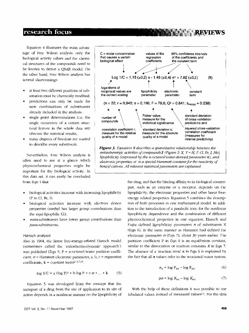
Equation 4 describes the antiadrenergic activities for 22

different m-, p- and m,p-disubstituted analogs of tile

N,N-dimethyl-a-bromophenethylamine 2 (Figure 2), where

C is the concentration that causes a 50% reduction of the

adrenergic effect of a certain epinephrine dose1.2,7; for the

meaning of r, s, F, and all other terms see Figure 3.

log 1/C = - 0.301 (_t_0.50) [m-F] + 0.207 (~_0.29) [m-C1]

+ 0.434 (~_0.27) [m-Br] + 0.579 (~0.50) [m-1]

+ 0.454 (~0.27) [m-Me] + 0.340 (_~_0.30) [p-F]

+ 0.768 (~0.30) [p-Cl] + 1.020 (_t_0.30) [p-Br] + 1.429

(k0.50) [p-I] + 1.256 (~_0.33) [p-me] + 7.821 (~_0.27)

(n = 22; r = 0.969; s = 0.194; F = 16.99) (4)

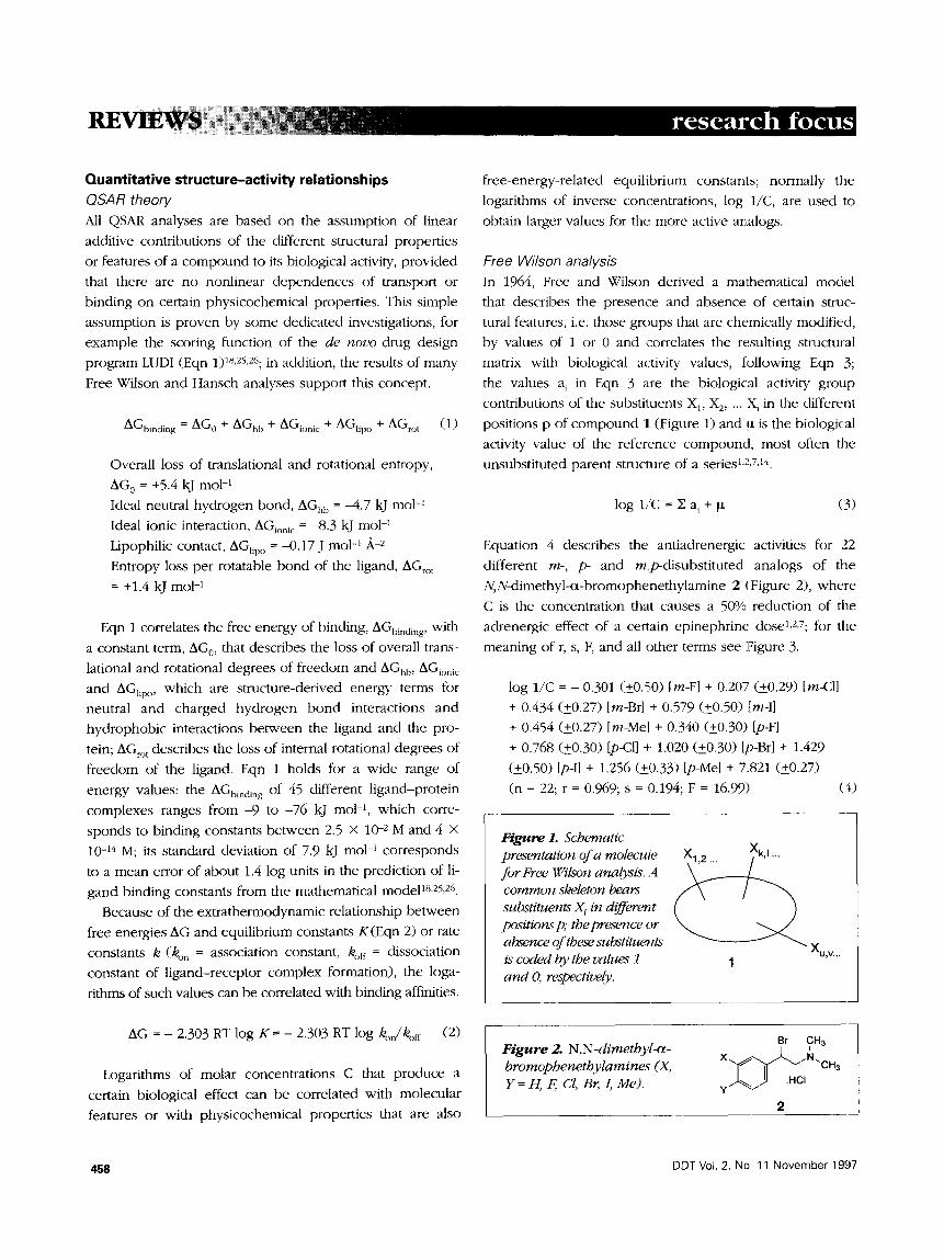
Figure 1. Schematic presentation of a molecule for Free Wilson analysis. A common skeleton bears substituents X i in different positions p, the presence or absence of these substituents is coded by the values 1 and O, respectively.

•• Xu,v...

1

Figure 2. N,N-dimethyl-a- bromophenethylamines (X, Y = H, F, CI, Br, I, Me).

Br CH3

"OH 3

Y 2

458 DDT Vol. 2, N o 11 November 1997

Equation 4 illustrates the main advan-

tage of Free Wilson analysis: only the

biological activity values and the chemi-

cal structures of the compounds need to

be known to derive a QSAR model. On

the other hand, Free Wilson analysis has

several shortcomings:

• at least two different positions of sub-

stitution must be chemically modified;

• predictions can only be made for

new combinations of substituents

already included in the analysis;

• single point determinations (i.e. the

single occurence of a certain struc-

tural feature in the whole data set)

obscure the statistical results;

• many degrees of freedom are wasted

to describe every substituent.

Nevertheless, Free Wilson analysis is

often used to see at a glance which

physicochemical properties might be

important for the biological activity. In

this data set, it can easily be concluded

from Eqn 4 that

C = molar concentration that causes a certain regression of the coefficients and biological effect coefficients the constant term

Log 1/C = 1 ,15 (+0 ,2 ) ~ - 1 .46 (-*0,4) o "+ + 7 .82 (+0 ,2)

l t \ logarithms of reciprocal values are lipophilicity electronic constant the correct scaling parameter parameter term

values of the 95% confidence intervals

(8)

(n = 22; r = 0 , 945 ; s = 0 ,196 ; F = 78 ,6 ; Q2 = 0 .841 ; SpREs s = 0 . 2 3 8 )

Fisher value; number of measure for the \ compounds statistical significance %

correlation coefficient r; standard deviation s; measure for the relative measure for the absolute quality of a model quality of a model

standard deviation of cross-validation predictions and

squared cross-validation correlation coefficient (measures for internal predictivity)

Figure 3. Equation 8 describes a quantitative relationship between the antiadrenergic activities of compounds2 (Figure 2; X, Y= H, F, CI, Br, I, Me), lipophilicity (expressed by the n-octanol/water-derived parameter zg), and electronic properties; o + is a special Hammett constant for the reactivity of benzyl cations. All relevant statistical parameters are explained.

• biological activities increase with increasing lipophilicity

(F to Cl, Br, I);

• biological activities increase with electron donor

properties (methyl has larger group contributions than

the equi-lipophilic Cl);

• meta-substituents have lower group contributions than

para-substituents.

Hansch analysis

Also in 1964, the linear free-energy-related Hansch model

(sometimes called the 'extrathermodynamic approach')

was published (Eqn 5; P = n-octanol/water partition coeffi-

cient, o = Hammett electronic parameter, a, b, c = regression

coefficients, k = constant term) 1-3,7,15.

l o g l / C = a ( l o g p ) 2 + b l o g P + c o + . . . + k (5)

Equation 5 was developed from the concept that the

transport of a drug from the site of application to its site of

action depends in a nonlinear manner on the lipophilicity of

the drug, and that the binding affinity to its biological counter-

part, such as an enzyme or a receptor, depends on the

lipophilicity, the electronic properties and other linear free-

energy-related properties. Equation 5 combines the descrip-

tion of both processes in one mathematical model. In addi-

tion to the introduction of a parabolic term for the nonlinear

lipophilicity dependence and the combination of different

physicochemical properties in one equation, Hansch and

Fujita defined lipophilicity parameters = of substituents X

(Eqn 6), in the same manner as Hammet: had defined the

electronic parameter o (Eqn 7), about 30 years earlier. The

partition coefficient P in Eqn 6 is an equilibrium constant,

similar to the dissociation or reaction constants K in Eqn 7.

The absence of a 'reaction term' = in Eqn 6 is explained by

the fact that all ax values refer to the n-octanol/water system.

=x = log Pmx - log Pen (6)

po = log KRx - log Ken (7)

With the help of these definitions it was possible to use

tabulated values instead of measured values 2,4. For the data

DDT Vol. 2, No. 11 November 1997 459

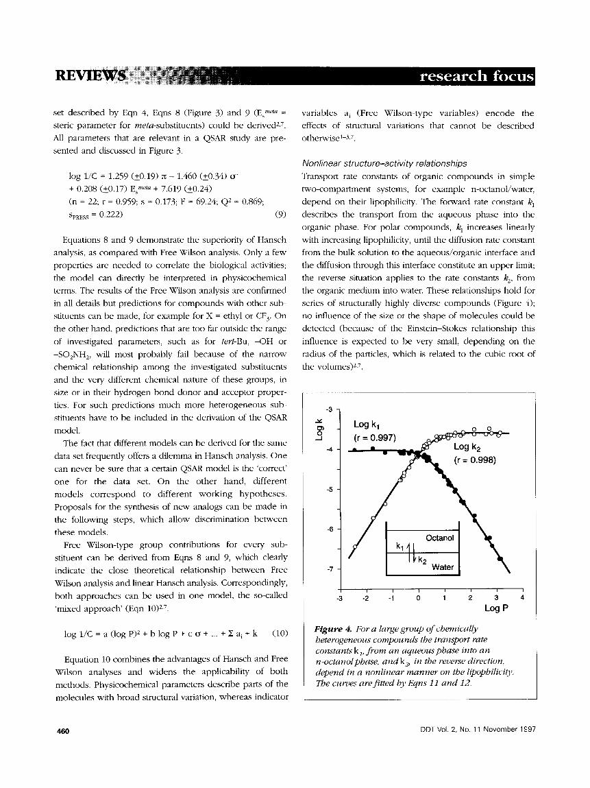
set described by Eqn 4, Eqns 8 (Figure 3) and 9 (Esmeta =

steric parameter for meta-substituents) could be derived 2,7.

All parameters that are relevant in a QSAR study are pre-

sented and discussed in Figure 3.

log 1/C = 1.259 (~_0.19) a~- 1.460 Ct0.34) o +

+ 0.208 (~_0.17) gs meta + 7.619 (&0.24)

(n = 22; r = 0.959; s = 0.173; F = 69.24; Q2 = 0.869;

SpRv:SS = 0.222) (9)

Equations 8 and 9 demonstrate the superiori W of Hansch

analysis, as compared with Free Wilson analysis. Only a few

properties are needed to correlate the biological activities;

the model can directly be interpreted in physicochemical

terms. The results of the Free Wilson analysis are confirmed

in all details but predictions for compounds with other sub-

stituents can be made, for example for X = ethyl or CF 3. On

the other hand, predictions that are too far outside the range

of investigated parameters, such as for tert-Bu, -OH or

-SO2NH2, will most probably fail because of the narrow-

chemical relationship among the investigated substituents

and the very different chemical nature of these groups, in

size or in their hydrogen bond donor and acceptor proper-

ties. For such predictions much more heterogeneous sub-

stituents have to be included in the derivation of the QSAR

model.

The fact that different models can be derived for the same

data set frequently offers a dilemma in Hansch analysis. One

can never be sure that a certain QSAR model is the 'correct'

one for the data set. On the other hand, different

models correspond to different working hypotheses.

Proposals for the synthesis of new analogs can be made in

the following steps, which allow discrimination between

these models.

Free Wilson-type group contributions for every sub-

stituent can be derived from Eqns 8 and 9, which clearly

indicate the close theoretical relationship between Free

Wilson analysis and linear Hansch analysis. Correspondingly,

both approaches can be used in one model, the so-called

'mixed approach' (Eqn 10) 2,7.

l o g l / C = a ( l o g p ) 2 + b l o g P + c o + . . . + X a i + k (10)

Equation 10 combines the advantages of Hansch and Free

Wilson analyses and widens the applicability of both

methods. Physicochemical parameters describe parts of the

molecules with broad structural variation, whereas indicator

variables a i (Free Wilson-type variables) encode tile

effects of structural variations that cannot be described

otherwise1-3,7.

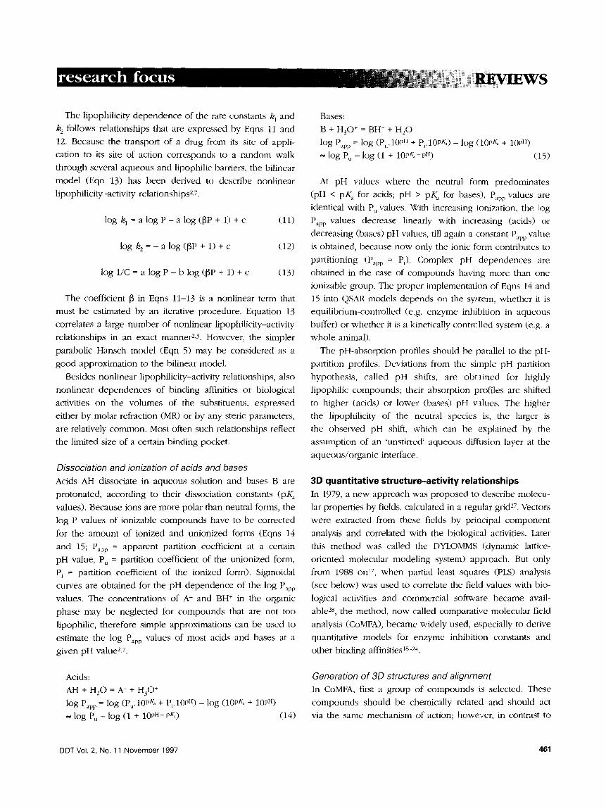
Nonlinear structure-activity relationships Transport rate constants of organic compounds in simple

two-compartment systems, for example n-octanol/water,

depend on tl~eir lipophilicity. The forward rate constant k 1

describes the transport from the aqueous phase into the

organic phase. For polar compounds, k I increases linearly

with increasing lipophilicity, until the diffusion rate constant

from the bulk solution to the aqueous/org;mic interface and

the diffusion through this interface constitute an upper limit;

the reverse situation applies to the rate constants k2, from

the organic medium into water. These relationships hold for

series of structurally highly diverse compounds (Figure 4);

no influence of the size or the shape of molecules could be

detected (because of the Einstein-Stokes relationship this

influence is expected to be very small, depending on the

radius of the particles, which is related to the cubic root of

the volumes) 2,7.

-3

q

- 4 •

- 6 ,

.7 ¸

-3

Log k 1 o o (r = 0 . 9 9 7 ) ~ ¢ ~ 6 ' t g - e - - e ~ 9 - - .. • • ~ = ~ Log k 2

i I I i I i

-2 -1 0 1 2 3 Log P

Figure 4. For a large group of chemically heterogeneous compounds the transport rate constants k l, f rom an aqueous phase into an n-octanol phase, and k2, in the reverse direction, depend in a nonlinear manner on the lipophilicity. The curves are fitted by Eqns 11 and 12.

460 DDT Vol. 2, No. 11 November 1£97

The lipophilicity dependence of the rate constants k 1 and

/e 2 follows relationships that are expressed by Eqns 11 and

12. Because the transport of a drug from its site of appli-

cation to its site of action corresponds to a random walk

through several aqueous and lipophilic barriers, the bilinear

model (Eqn 13) has been derived to describe nonlinear

lipophiliciW-activi W relationshipsa, 7.

l o g k l = a l o g p - a l o g ( 1 3 P + 1 ) + c (11)

log k 2 = - a log (13P + 1) + c (12)

log 1/C = a log P - b log (13P + 1) + c (13)

The coefficient [3 in Eqns 11-13 is a nonlinear term that

must be estimated by an iterative procedure. Equation 13

correlates a large number of nonlinear lipophilicity-activity

relationships in an exact manner2, 3. However, the simpler

parabolic Hansch model (Eqn 5) may be considered as a

good approximation to the bilinear model.

Besides nonlinear lipophilicity-activity relationships, also

nonlinear dependences of binding affinities or biological

activities on the volumes of the substituents, expressed

either by molar refraction (MR) or by any steric parameters,

are relatively common. Most often such relationships reflect

t h e limited size of a certain binding pocket.

Dissociation and ionization of acids and bases Acids AH dissociate in aqueous solution and bases B are

protonated, according to their dissociation constants (pK,

values). Because ions are more polar than neutral forms, the

log P values of ionizable compounds have to be corrected

for the amount of ionized and unionized forms (Eqns 14

and 15; Papp = apparent partition coefficient at a certain

pH value, Pu = partition coefficient of the unionized form,

P~ = partition coefficient of the ionized form). Sigmoidal

curves are obtained for the pH dependence of the log Papp

values. The concentrations of A- and BH ÷ in the organic

phase may be neglected for compounds that are not too

lipophilic, therefore simple approximations can be used to

estimate the log Papp values of most acids and bases at a

given pH value 2,7.

Acids:

AH + H20 = A- + H30+ log Papp = log (Pu.10PK~ + Pi.10pFI) - log (10PK~ + 10P H)

-~ log Pu - log (1 + 10P u - P&) (14)

Bases:

B + H30 + = BH ÷ + H20

log Papp = log (Pu.10PH + Pi.10PK~)- log (10P& + 10P H)

log Pu - l o g (1 + 10P/(~ - pH) (15)

At pH values where the neutral form predominates

(pH < pK, for acids; pH > pK~ for bases), Papp values are

identical with Pu values. With increasing ionization, the log

Papp values decrease linearly with increasing (acids) or

decreasing (bases) pH values, till again a ,constant Papp va]ue

is obtained, because now only the ionic form contributes to

partitioning (Papp = Pi )' Complex pH dependences are

obtained in the case of compounds having more than one

ionizable group. The proper implementation of Eqns 14 and

15 into QSAR models depends on the system, whether il is

equilibrium-controlled (e.g. enzyme inhibition in aqueous

buffer) or whether it is a kinetically controlled system (e.g. a

whole animal).

The pH-absorption profiles should be parallel to the pH-

partition profiles. Deviations from the simple pH partition

hypothesis, called pH shifts, are obtained for highly

lipophilic compounds; their absorption profiles are shifted

to higher (acids) or lower (bases) pH values. The higher

the lipophilicity of the neutral species is, the larger is

the observed pH shift, which can be ,explained by the

assumption of an 'unstirred' aqueous diffusion layer at the

aqueous/organic interface.

3D quantitative structure-activity relationships In 1979, a new approach was proposed to describe molecu-

lar properties by fields, calculated in a regular grid 27. Vectors

were extracted from these fields by principal component

analysis and correlated with the biological activities. Later

this method was called the DYLOMMS (dynamic lattice-

oriented molecular modeling system) approach. But only

from 1988 o n 17, when partial least squares (PLS) analysis

(see below) was used to correlate the field values with bio-

logical activities and commercial software became avail-

able 28, the method, now called comparative molecular field

analysis (CoMFA), became widely used, especially to derive

quantitative models for enzyme inhibition constants and

other binding affinities 1~24.

Generation of 3D structures and alignment In CoMFA, first a group of compounds is selected. These

compounds should be chemically related and should act

via the same mechanism of action; however, in contrast to

DDT Vol. 2, No. 11 November 1997 461

classical QSAR methods, they should have a c o m m o n

pha rmacophore , not necessarily the same molecular skel-

eton. As the pha rmacophore refers to 3D structures, first the

2D or 2.5D (including configurational information) struc-

tures of all molecules are converted to 3D structures.

Standard computer programs for this purpose are CON-

CORD (Ref. 29) and CORINA (Ref. 30). However, both pro-

grams create only one low-energy structure per molecule.

Most often one or several torsion angles of flexible mol-

ecules have to be modified (of course, leading to other low-

energy 3D structures) to derive a c o m m o n pha rmacophore

for all analogs. The investigation of rigid analogs or analogs

with different conformational constraints helps to find or

confirm the 'bioactive' conformations of the more flexible

molecules.

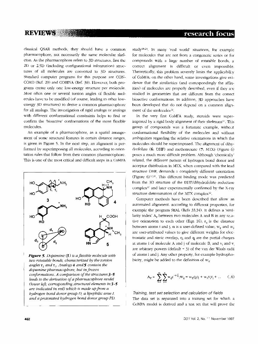
An example of a pharmacophore , as a spatial arrange-

ment of some structural features in certain distance ranges,

is given in Figure 5. In the next step, an alignment is per-

formed by super imposing all molecules, according to orien-

tation rules that follow from. their c o m m o n pharmacophore .

This is one of the most critical and difficult steps in a CoMFA

H O ~ NH3 H~HCH3

HOAI"~JlI:'3 1:, HO + 4

. ~ ~ ' ~ NH3

HO" ~" . o

d ~ d z ~'CH3 d3 HN 5

H COOH

Figure 5. Dopamine (3) is a flexible molecule with two rotatable bonds, characterized by the torsion angles T 1 and J;2. Analogs4 a n d 5 contain the dopamine pharmacophore, but in frozen conformations. A comparison of the structures3-5 leads to the derivation of a pharmacophore model (lower left; corresponding structural elements in 3 - 5 are indicated in red) which is made up from a hydrogen bond donor group D, a lipophilic area L and a protonated hydrogen bond donor group PD.

study 1&24. In many 'real world ' situations, for example

for molecules that are not from a congeneric series or for

c o m p o u n d s with a large number of rotatable bonds, a

correct a l ignment is difficult or even impossible.

Theoretically, this problem severely limits the applicabili.-y

of CoMFA; on the other hand, some investigations give evi-

dence that the similarities (and correspondingly the affin-

ities) of molecules are properly described, even if they a:e

studied in geometries that are different from the correct

bioactive conformations. In addition, 3D approaches have

been developed that do not depend on a c o m m o n alig:'l-

ment of the molecules 24.

In the very first CoMFA study, steroids were super-

imposed by a rigid b o d y alignment of their skeletons 17. Tlqs

g roup of c o m p o u n d s was a fortunate example, withoat

conformational flexibility of the molecules and without

ambiguities regarding the relative orientations in which the

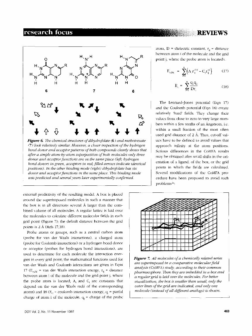
molecules should be superimposed. The alignment of dihy-

drofolate (6; DHF) and methotrexate ('7; MTX) (Figure 6)

poses a much more difficult problem. Although 'chemically'

related, the different pattern of hydrogen b o n d donor and

acceptor distribution in MTX, w h e n compared with the lead

structure DHF, demands a completely different orientation

(Figure 6)~2.3L This different binding mode was predicted

from the 3D structure of the DHF/dihydrofolate reductase

complex3~ and later experimentally confirmed by the X-ray

structure determination of the MTX complex32.

Computer methods have been described that allow an

au tomated alignment, according to different properties, for

example the program SEAL (Refs 33,34). It defines a 'simi-

larity index' A v between two molecules A and B in any re:a-

tive orientation to each other (Eqn 16); qi is the distance

be tween atoms i and j, ct is a user-defined value, w E and w s

are user-attributed values to give different: weights for elec-

trostatic and steric overlap, qi and qi are the partial charges

at atoms i of molecule A and j of molecule B, and v i and v i

are arbitrary powers (default = 3) of the van der Waals radii

of atoms i and j. Any other property, for example hydropho-

biciW, might be added to the definition of w~i.

~__ ~ -c~ A F = wije 'J ;wij = WEqiq j + WsViV j + ... (26)

]=1

Training, test set selection and calculation of fields

The data set is separate(] into a training set for which a

CoMFA model is derived and a test set that will prove 1:he

462 DDT Vol. 2, No. 11 November 1997

0 H ' N ' H H ' N I ~ f

""'<'"" " i I I I I I I

H H H H H H

6 7 6

R

M M t t K K #

¢ q 6 4 , ¢ ¢ 1 , ¢ ¢ Figure 6. The chemical structures of dihydrofolate (6) and methotrexate (7) look relatively similar. However,, a closer inspection of the hydrogen bond donor and acceptor patterns of both compounds clearly shows that after a simple atom-by-atom superposition of both molecules only three donor and acceptor functions are in the same place (left; hydrogen bond donors in green, acceptors in red,. filled arrows indicate identical positions). In the other binding mode (right) dihydrofolate has six donor and acceptor functions in the same place. This binding mode was predicted and several years later experimentally confirmed.

atom, D = dielectric constant, % = distance

be tween atom i of the molecule and the grid

point j, where the probe atom is located}

n

E a w = ' ~ ( A r 7 1 2 _ C r - 6 ) ~ , t \ ~ 11 i ij i=1

(17)

& q ,q , E C = y

Lai=l Dri i (18)

The Lennard-Jones potential (Eqn 17)

and the Coulomb potential (Eqn 18) create

relatively 'hard' fields. They change their

values from close to zero to very large num-

bers within a few" tenths of an Angstrom, i.e.

within a small fraction of the most often

used grid distance of 2 A.. Thus, cut-off val-

ues have to be defined to avoid values that

approach infinity at the atom positions.

Serious differences in the CoMFA results

may be obtained after small shifts in the ori-

entation of a ligand, of the box, or the grid

points in which the fieMs are calculated.

Several modifications of the CoMFA pro-

cedure have been proposed to avoid such

problems24:

external predictivity of the resulting model. A box is placed

around the super imposed molecules in such a manner that

the box is in all directions several ~ larger than the com-

bined volume of all molecules. A regular lattice is laid over

the molecules to calculate different molecular fields in each

grid point (Figure 7); the default distance be tween the grid

points is 2 A (Refs 17,18).

Probe atoms or groups, such as a neutral carbon atom

(probe for van der Waals interactions), a charged a tom

(probe for Coulomb interactions) or a hydrogen b o n d donor

or acceptor (probes for hydrogen b o n d interactions), are

used to determine for each molecule the interaction ener-

gies in every grid point; the mathematical functions used for

van der Waals and Coulomb interactions are given in Eqns

17 (E,,dw = van der Waals interaction energy, r~i = distance

between atom i of the molecule and the grid point j, where

the probe atom is located; A~ and C i are constants that

depend on the van der Waals radii of the cor responding

atoms) and 18 (E c = cou lomb interaction energy, qi = partial

charge of a tom i of the molecule, qi = charge of the p robe

1 ~ 5 . 5 - 5 - ~ 5 - ~ 5 - ~ 5 - ~ I I

f f f f f f f f f f f f f

A |

I I I ~ " ~ _

IP~- I . ~ ' ~ ~

Figure 7. All molecules of a chemically related series are superimposed in a comparative molecular f ieM analysis (CoMFA) study according to their common pharmacophore. Then they are imbedtled in a box and a regulargrid is laid over the molecules. For better visualization, the box is smaller than usual, only the ouwr lines of the grid are indicated, a, nd only one molecule (instead of all different analogs) is" shown.

DDT Vol. 2, No. 11 November 1997 463

• a cross-validated QX-guided region selection to achieve

consistent results 35,

• reorientations of the molecules for which too low activ-

ities are calculated, to obtain an ' improved' (but more

subjective) al ignment 36,

• single and domain m o d e variable selection in the PLS

analysis 37, and

• a selection of relevant regions by the GOLPE variable

selection program 38.

In a recent CoMFA modification, called comparat ive mol-

ecular similari W indices analysis (CoMSIa) 24,39, SEAL func-

tions (Eqn 16) are used to calculate 'similari W fields' ta

probe atoms and groups, in the same manner as CoME~_

fields are calculated. Since the CoMSIA fields are Gaussian

potentials, they are much 'softer' than the CoMFA functions. In

addition, they are g o o d approximations to the cut-off-

corrected Lennard-Jones and Coulomb potentials (Figure 8 I.

As expected, CoMSIA fields have been shown to p roduce

smoother contour maps (see below) than CoMFA fields 39.

Correlation of the molecular fields with th,e biological data The resulting matrix of several thousand columns of the

individual grid point values for each molecule cannot be

correlated by regression analysis. Partial least squares (PLS)

I Lennard-Jones I potential, CoMFA

cut-off value

Gaussian , ~ approximation, Coulomb CoMSIA potential, CoMFA

(identical charges)

>

r

Gaussian / Coulomb approximation, potential, CoMFA CoMSIA (different charges)

cut-off value

Figure 8. The Lennard--Jones and Coulomb functions are 'hard'potentials. Within several tenths of an Angstrom they change their values from close to zero to very large values. Cut-off values have to be defined to avoid such unreasonably large values. The comparative molecular similarity indices analysis (CoMSIA) potentials are much smoother,, the}, may be considered as good approximations for the cut-off- limited Lennard-Jones and Coulomb potentials in CoMFA (comparative molecular f ield analysis).

Y vector X matrix

BA 1 BA 2 BA 3

$11 $12 $21 S22 $31 $32

Snl Sn2

$13 S14 . . . . . Slm Ell Eli 2 . . . . . Elm S23 S24 . . . . . S2m E21 E.q2 . . . . . E2m S33 Sa4 . . . . . S3m E31 E32 . . . . . E3m

; : : ; l l

: • . . . . . : : : . . . . :

: : : : • .

• : • : : :

S3n Sn4 . . . . . Snm Enl En2 . . . . . Enm

! PLS analysis

u111 t l l I t21 u121 t12 t22 u131 t113[] t23 .: , I - -

• o

Ul n : : tln t2n ....

PLS vectors (latent variables)

SAMPLS analysis

Cll c21 c31 . . . . Cnl c21 c22 c32 . . . . Cn2 c31 c32 c33 . . . . Cn3

Cnl Cn2 Cn 3 . . . . Cnn

covariance matrix

Figure 9. Partial least squares (PLS) analysis extracts principal component-like vectors (so-called latent variables)from the F block (biological data; usually only a y vector) a n d the X block (in comparative molecular field analysis the field variables in the d!lCferent grid points). SAMPLS analysis k; a PLS variant, in which a covariance matrix h; calculated

f rom theX block a n d the latent variables are derived f rom this matrix. PLS and SA!VIPLS analysis give absolutely identical results, with the advantage that SAMPLS is some orders qf magnitude faswr in cross- validation runs.

464 DDT Vol. 2, No. 11 November 1997

Xl

From u = kt (k = constants k~, k 2 ... kj; j = number of PLS vectors)

follows:

BA~ = alSil + a2Si2 + a3Si3 + ... + arnSim + + blEil + b2E ~ + b3Ei3 + ... + bmEim

Figure 10. The main advantage of PLS analysis, as compared with principal component regression analysis is the fact that PLS vectors (dotted line) are shifted against the principal components (bold line), in order to achieve a maximum correlation between the Y and theX block,, the tube indicates the confidence volume of the principal component.

analysis is the method of choice (Figure 9). This method

extracts principal component-like vectors, the so-called

latent variables, from the Y block (usually only a one-

column vector y) and the X block; the latent variables

are shifted within the confidence volumes of the principal

components, in such a manner that a maximum correlation

between these variables, called u and t, is achieved

(Figure 10) 2,5,<1s.

The optimum number of latent variables is determined by

cross-validation 2,5,<~s. In this approach, many models are

derived where one or several compounds are excluded from

the data set and are predicted by the corresponding model.

In the most common 'leave-one-out' cross-validation, every

compound is eliminated once. Thus, n models

(n = number of compounds) are derived and the n predic-

tions are compared with the experimental values; Q2, the

squared cross-validated correlation coefficient, and s~,Ress,

the standard deviation of predictions, are calculated from

the sum of the squared deviations of the predicted values

(PRESS), in the same manner as the squared correlation

coefficient r 2 and the standard deviation s are calculated if

no cross-validation is performed. Most often, the highest Q2 or the lowest SpRES s is taken as the criterion for the optimum

number of latent variables. For theoretical reasons, Q2

cannot be larger than r 2 and SpRES s cannot be smaller than s;

Q2 may even be negative, which means that the predictions

by the model are worse than taking the average of all bio-

logical data as the predictions.

The result of a PLS analysis corre-

sponds to a regression equation with

thousands of coefficients, from which

predictions for compounds outside the

investigated training set can be made.

Most often the PLS results are presented

as contour plots; favorable and unfavor-

able regions for certain properties in

space are indicated in different colors

(Figure 11) 4°. Since 1988, a few hundred publi-

cations, several reviiews ~9-23 and two

books 18,24 have appeared on this sub-

ject. Unfortunately, several CoMFA

studies do not meet all necessary scien-

tific and statistical standards. Critical

reviews on the validity of the results

and conclusions of CoMFA studies have

been published is,>. Despite some

major problems in its proper application, the method is now

generally accepted as a useful tool for .deriving 3D QSAR

models.

Q u a n t i t a t i v e s i m i l a r i t y - a c t i v i t y r e l a t i o n s h i p s ( Q S i A R )

Similar molecules, having similar structures and similar

physicochemical properties, are supposed to have also simi-

lar biological properties and comparable activity values.

Whereas there are some significant exceptions to this gen-

eral assumption, it is the basis of all quantitative structure-

activity relationships. Quantitative similarity-activity

relationships (QSiAR) correlate the degree of mutual simi-

larity of all molecules within a series with their biological

activities.

Rum and Herndon, in 1991, used n × n similarity index

matrices (n = number of compounds in the data set), derived

from 2D topological descriptors, and s'tepwise regression

analysis to correlate several columns of these matrices with

biological activities 41. Two years later, in a more systematic

investigation, Good and Richards superimposed molecules,

like in CoMFA analyses, and compared their 3D electronic

similarity42, 43. The resulting n X n similarity index matrices

were correlated with biological activities, using either neural

networks or PLS analysis.

This concept could be extended to many other linear and

nonlinear QSiAR relationships, by calcu].ating either n x n

distance matrices D (especially suited for nonlinear relation-

ships) or n X n covariance matrices C as similarity

DDT Vol. 2, No. 11 November 1997 465

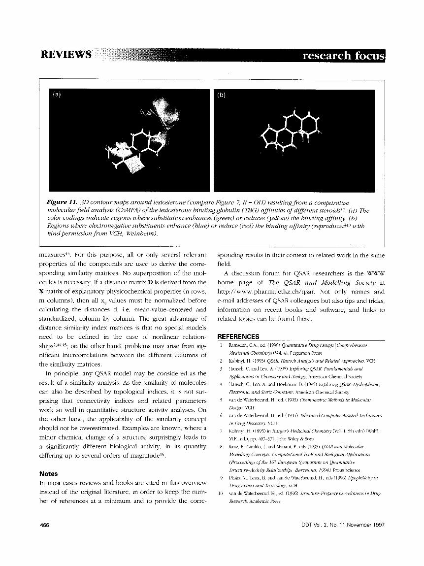
REVIEWS!

(b)

F i g u r e 11. 3 D con tour maps a r o u n d testosterone (compare Figure Z R = OH) result ing f r o m a comparat ive molecu lar f i e ld analysis (CoMFA) o f the testosterone b ind ing globul in (TBG) aff init ies oJ'different steroid.s qT. (a) The color codings indicate regions where subst i tut ion enhances (green) or reduces (yellow) 1he b ind ing affiniO,. (b) Regions where electronegative subst i tuents e n h a n c e (blue) or reduce (red) the b ind ing affi'ni O, ( reproduced 4o with k ind permiss ion f i 'om VCH, Weinbeim) .

measures 4~. For this purpose, all or only several relevant

properties of the compounds are used to derive the corre-

spond ing similarity matrices. No superposi t ion of the mol-

ecules is necessary. If a distance matrix D is derived from the

X matrix of explanatory physicochemical properties (n rows,

m columns), then all x~i values must be normal ized before

calculating the distances d, i.e. mean-va lue-centered and

standardized, co lumn by column. The great advantage of

distance similarity index matrices is that no special models

need to be defined in the case of nonl inear relation-

ships2'44,45; o n the other hand, problems may arise from sig-

nificant intercorrelations be tween the different columns of

the similarity matrices.

In principle, any QSAR model may be considered as the

result of a similarity analysis. As the similarity of molecules

can also be described by topological indices, it is not sur-

prising that connectivity indices and related parameters

work so well in quantitative structure-activity analyses. On

the other hand, the applicability of the similarity" concept

should not be overestimated. Examples are known, where a

minor chemical change of a structure surprisingly leads to

a significantly different biological activity, in its quanti ty

differing up to several orders of magni tude ~6.

Notes In most cases reviews and books are cited in this overview

instead of the original literature, in order to keep the num-

ber of references at a m in imum and to provide the corre-

spond ing results in their context to related work in the same

field.

A discussion forum for QSAR researchers is the grWW

home page of The QSAR a n d Mode l l ing Socie ty at

h t t p : / / w w w . p h a r m a . e t h z . c h / q s a r . Not only names ar,d

e-mail addresses of QSAR colleagues but also tips and tricks,

information on recent books and software, and links ~o

related topics can be found there.

REFERENCES 1 Ramsden, C.A., ed. (1990) Quantitative Dntg Deszgn (Comprehenszve

Medicinal Cbemistr39 (Vol. 4), Fergamon Press 2 Kubinyi, H. (1993) QSAR: Hansch Analysis and RelatedApproacbes, VCH 3 Hansch, C. and Leo, A. (1995) Exploring QSAR. Fund~onentals and

Applications in Chemist O' and 3ioloRv, American Chemical Society 4 Hansch, C., Leo. A. and Hoekm:m, D. (1995) Exploring QSAR. Hydropbobi<

Electronic, and Steric Constant::, American Chemical Society 5 van de ~,'aterbeemd, H, ed. (19'95) Chemometrt'c Methods in Molecular

Design, VCH

6 van de \Vaterbeemd, H., ed. (19'95) Advanced Compme~=Assisted Techniques in Dn~g Dfscoveo'. VCH

7 Kubinyi, H. (1995) in Burger's Medicinal Chemistrl, (\'ol. 1, 5th edn) (Wolff, M.E.. ed.), pp. 497-571, John Wiley & Sons

8 Sanz, F., Giraldo, J. and Manaut, F, eds (1995) QSAR and Molecular Modelling: Concepts. Computat~.onal Tools and Biolqgical Applications (Proceedi~gs of the 10 I' European Symposium on Quantitative Structttre~Activity Relationsbip.,; Barcelona. 1994), Prous Science

9 Pliska, V., Testa, B. and van de Waterbeemd, H, eds (19%) Ll~ophilicity in Drug Action and Toxicolog3,, VCH

10 van de Waterbeemd. H.. ed (1996) Structmz~Propertl, Co~-relations in DzTtg Research, Academic Press

466 DDT Vol. 2, No, 11 November 1997

11 van de Waterbeemd, H. (1996) in The Practice of Medicinal Chemistry

(Wermuth, C.G., ed.), pp. 367-389, Academic Press

12 B6hm. H-J., Klebe, G. and Kubinyi, H. (1996) Wwhsto]ybtes~gn, pp. 363-380

and 399-436, Spektmm Akademischer Verlag

13 van de Waterbeemd, H., Testa, B. and Folkers, G., eds (1997) Compute~=

assisled Lead Finding and Optimization (Proceedings of the IF ~' Earopean

Symposium on Quantitative Structure-Activity Relationships: Lausanne,

1996), Verlag Helvetica Chimica Acta and VCH

14 Free, S.M., Jr and Wilson, J.W. (1964).L Med Chem. 7, 395-399

15 Hansch, C. and Fujita, T. (1964) J. Am Chem. Soc. 86. 1616-1626

16 Kubinyi, H (1997) Drag Discove O' To&(v 2, part 2

17 Cramer. RD., III. Patterson, D.E and Bunce, J.D. (1988) J Am. Cbem 5~c.

110, 595%5967

18 Kubinyi, H., ed. (1993) 3D QSAR in Drug Design. Theory, Metbods and

Applications, ESCOM Science Publishers

19 Green, S.M and Marshall, G.R. (1995) TrendsPharmacol. Sci. 16. 285-291

20 Kim, K.H. (1995) in Molecular Similari(i, in Drug Design (Dean. P.M., ed.),

pp. 291-331, Chapman & Hale

21 Martin. Y.C. and Lin, C.T. (1~)6) in The Practice of Medicinal Chemistry

(Wermuth, C.G., ed.), pp. 459-483, Academic Press

22 Blankley, C.J. (1996) in Stntcture-Prope~l' Correlations in Drug Research

(van de Waterbeemd, H., ed), pp. 111-177, Academic Press

23 Martin, Y.C., Kim, K-H. and Lin, C.T. (1996) in Adz,antes in Quantitative

Stn+cture Propeqv Relationships (\:ol. I) (Charton, M., ed.), pp. 1-52, JAI Press

24 Kubinyi, H., Folkers, G. and Martin, Y.C., eds (1997) 3D QSAR in Dpv¢g

Design Ligand-Protein Interactions and Molecular SimilanO; (Vol. 2) and

Recent Aduances (Vol. 3), Kluwer Academic Publishers

25 B6hm, H-J. (1994)J. Comput.-AidedMol. Design 8, 243-256

26 B6hm, H-J. and Klebe, G. (1996) Angeu'. Chem. 108, 2750-2778, Angew.

Chem., Int. Eel. Engl. 35, 2588-2614

27 Cramer. RD.. [I[ and Milne, M. (1979) Am. Chem. Soc. Meeti,g, April 1979,

Computer Chemis W Section. Abstr. no. 44

28 SYBYL/QSAR, Molecular Modelling Soft'are, Tripos Inc., 1699 S. Hanley

Road, St Louis, MO 63944, USA

29 Pearlman, R.S. (1993) Chem. Design Automation ATeu's8 (8), 3-15

30 Sadowski, J. and Gasteiger, J. (1993) Chem. Rev. 93, 2567-2581

31 Bolin, J.T. et al. (1982) J. Bfol. Chem. 257, 13650-13662

32 Bystroff, C., Oatley, S.J. and Kmut, J. (1990) Biochemistry 29, 3263-3277

33 Kearsley, S.K. and Smith, G M (1990) Tetrahedron Comput Methodol. 3,

615433

34 Klebe, G.. Mietzner, T. and Weber, F. (1994) J. Comput.-AidedMol. Design 8,

751-778

35 Cho, S.J. and Tropsha, A. (1995) J Med. Chem 38, 1060-1066

36 Kroemer, R.T. and Hecht, P. (1995).L Comput-dMedMol. Design 9.

396-4O6

37 Norinder, U. (1996)J. Chemomet. 10, 95-105

38 Cmciani, G., Pastor, M. and Clementi, C. (1997) in G)mpute~,Assisted Lead

Finding and Optimization {Proceedings of the l l #~ ~uropean Symposium on

Quantitatize Sh~+cture~Activi(;; Relationships, Laus~mn< 1996) (van de

Waterbeemd, H., Testa, B. and Folkers, G., eds), pp. 379-395, Verlag Helvetica

Chimica Acta and VCH

39 Kletxt, G., Abraham, U. and Mietzner, T. C1994).L Med. Chem. 37. 4130-~146

40 Kubinyi, H. (1994) Chemie in uzzsererZeit 23, 281-290

41 Rum, G. and Herndon, W.C. (1991)5 Am. Chem. So:'. 113, 9055-9060

42 Got×l, A.C., Peterson, SO. and Richards, WG. (1993) J. Med. Chem. 36,

2929-2937

43 Good, A.C. (1995) in Mulecuh~r Similari(y in Drug L)esl~gn (Dean, P.M., ed),

pp. 24-56, Chapman & Hall

44 Kubinyi, H. (1997) in Computer-Assisted Lead Finding and Optimization

(Proceedings of the IF ~' European 5)'mpm'ium on Quantitative

Stntcture.-Activi o, Relationships, Lausanne. 1996)(,;an de Waterbeemd, tt.,

Testa, B. and Folkers, G.. eds), pp. 7-28, Verlag Hel,~etica Chimica Acta and

vcIq

45 Martin, Y.C. et al. (1995)J. Med Chem. 38, 3009-3015

In t h e D e c e m b e r issue of D r u g D i s c o v e r y Today.. .

Update- latest news and views

Accelerating drug discovery: creating the right environment Steve Arlington

Appfication of biocatalysis and biotransformations to the synthesis of pharmaceuticals Aleksey Zaks and David R. Dodds

HPLC-API/MS/MS: a powerful toot for integrating drug metabolism into the drug discovery process Walter A. Korfmacher, Kathleen A. Cox, Matthew S. Bryant, John Veals, Kwokei Ng, Robert Watkins and

Chin-Chung Lin

QSAR and 3D QSAR in drug design. Part 2: applications and problems Hugo Kubinyi

Monitor- new bioactive molecules, high-throughput screening, combinatorial chemistry, emerging molecular targets

DDT Vol. 2, No. 11 November 1997 467