p. 1

PPRROODDUUCCTTIIOONN OOFF NNOONN WWOOVVEENN

MMAATTEERRIIAALLSS FFOORR

BBIIOOTTEECCHHNNOOLLOOGGIICCAALL AAPPPPLLIICCAATTIIOONNSS

VVIIAA EELLEECCTTRROOSSPPIINNNNIINNGG

Dott. Luigi Sabetta

Dottorato in Scienze Biotecnologiche – XX ciclo Indirizzo Biotecnologie Industriali Università di Napoli Federico II

p. 2

p. 3

Dottorato in Scienze Biotecnologiche – XX ciclo Indirizzo Biotecnologie Industriali Università di Napoli Federico II

PPRROODDUUCCTTIIOONN OOFF NNOONN WWOOVVEENN

MMAATTEERRIIAALLSS FFOORR

BBIIOOTTEECCHHNNOOLLOOGGIICCAALL AAPPPPLLIICCAATTIIOONNSS

VVIIAA EELLEECCTTRROOSSPPIINNNNIINNGG

Dott. Luigi Sabetta

Dottorando: Dott. Luigi Sabetta

Relatore: Prof. Stefano Guido

Coordinatore: Prof. Giovanni Sannia

p. 4

p. 5

Ai miei genitori.

p. 6

p. 7

Summary

Summary .................................................................................................................... 7

Abstract ...................................................................................................................... 9

Riassunto .................................................................................................................. 10

Chapter 1 STATE OF THE ART OF THE ELECTROSPINNING PROCESS ........... 16 1 Introduction ................................................................................................................... 16

2 Historical Background ................................................................................................... 17

3 Electrospinning Theory and Process .............................................................................. 19

4 Bending instability ......................................................................................................... 21

5 Process parameters and fiber morphology ...................................................................... 25

6 Solution parameters and fiber morphology ..................................................................... 27

7 Aim of this thesis ........................................................................................................... 28

Chapter 2 Materials and Methods ............................................................................. 30 1 Experimental apparatus .................................................................................................. 30

2 Methods to generate oriented electrospun nanofibers ..................................................... 31

3 Materials ........................................................................................................................ 36

3.1 Poly-ethylene-oxide (PEO) ..................................................................................... 36

3.2 Poly-L-lactide (PLA) .............................................................................................. 38

3.3 Poly(ε-caprolactone) (PCL) ..................................................................................... 42

3.4 Hyaluronic acid (HA) .............................................................................................. 44

Chapter 3 Electrospinning of benzyl ester of hyaluronic acid (HYAFF-11) ............... 46 1 Introduction ................................................................................................................... 46

2 Fabrication of HYAFF-11 scaffolds ............................................................................... 46

3 Fiber characterization .................................................................................................... 48

4 Cell culture and seeding ................................................................................................. 51

5 Cell proliferation studies ................................................................................................ 54

6 Conclusions ................................................................................................................... 59

Chapter 4 DISPERSION OF NANOPARTICLES BY ELECTROSPINNING PROCESS ................................................................................................................ 60

1 Introduction ................................................................................................................... 60

2 Sepiolite ........................................................................................................................ 60

3 Preliminary work ........................................................................................................... 61

4 Fabrication of scaffolds made from HPC-PEO blends containing sepiolite ..................... 62

5 Conclusion ..................................................................................................................... 64

Chapter 5 Collagen Gel Assay for Tissue Cell Chemotaxis ...................................... 65 1 Introduction ................................................................................................................... 65

2 Material and methods ..................................................................................................... 67

2.1 Cell culture. ............................................................................................................ 67

2.2 Chemotaxis chamber. .............................................................................................. 67

2.3 Preparation of chemotaxis assays. ........................................................................... 68

2.4 Collagen gel birefringence ...................................................................................... 68

2.5 CF concentration profile measurements. .................................................................. 69

3 Preparation of trans-epithelial assays by the electrospinning process .............................. 71

4 Results ........................................................................................................................... 73

4.1 Jurkat cells .............................................................................................................. 75

4.2 Fibrosarcoma cells .................................................................................................. 82

4.3 Lymphocyte Mononuclear cells .............................................................................. 86

p. 8

5 Conclusion ..................................................................................................................... 92

BIBLIOGRAPHY ....................................................................................................... 93

Appendix ................................................................................................................... 99

p. 9

Abstract Electrospinning is a process by which a polymer solution or melt can be spun into submicron fibers by using a high potential electric field. Based on earlier research results, the average diameter of electrospun fibers ranges from 100 nm to a few microns. The advantages of the electrospinning process are its technical simplicity and its versatility. The apparatus used for electrospinning consists of a high voltage electric source with positive or negative polarity, a syringe or pipette feeding the solution by means of a syringe pump, and a conducting collector like aluminum. The collector can be made of any desired shape, like a flat plate, rotating drum, etc. This work can be divided in four parts. In the first one a review of literature is done with a special emphasis on the methods to develop an electrospinning apparatus and on possible applications. Furthermore, the apparatus set up is performed and tested by using polymer solutions widely described in the literature, such as polylactid acid (PLA), polycaprolactone (PCL) and polyethylenoxide (PEO). Different configurations of the apparatus were devised in order to obtain cylindrical and unixially aligned fiber scaffolds. In the second part, the electrospinning apparatus was used to fabricate nano/micro fibrous scaffolds of an ester of (HYAFF-11). The industrial interest in this material, which has never been electrospun before, is due to its biomedical properties combined with a slower in vivo degradation rate as compared to hyaluronic acid. The effects of solution properties and processing parameters on the structure and morphology of the electrospun HYAFF-11 membranes are thoroughly investigated to find the optimal processing conditions. The results show that the morphology of the electrospun fibers depends on the strength of the applied electric field and on the solution viscosity (i.e, concentration). The diameter of the nanofibers decreases with electrospinning voltage. It is found that higher solution concentrations favour the formation of uniform nanofibers with no bead-like defects. We have also studied cell proliferation on electrospun HYAFF-11 scaffolds in comparison with electrospun PLA and PCL scaffolds. It is found that cell proliferation on electrospun HYAFF-11 scaffolds is faster as compared to the other electrospun scaffolds. In the third part of the thesis the electrospinning process is used to fabricate polymer nanofibers containing one-dimensional arrays of sepiolite (SEP) nanoparticles. SEP is industrially-relevant ceramic porous clay with biotechnological applications in composite materials. One of the main challenges in dispersing nanoparticles in a continuous phase is to avoid formation of aggregates. Our approach is to use electrospinning as a way of dispersing SEP at the nanoscale. A blend obtained by mixing solutions of PEO with solutions of hydroxylproylcellulose (HPC) has been successfully used as a template to arrange the SEP nanoparticles within the fibers during electrospinning and the results have been assessed by TEM. In the last part of this thesis we present how electrospun scaffolds could be used to improve a novel assay to study cell migration and chemotaxis in a direct-viewing chamber. In the chemotaxis assay presented in this work a chemoattractant concentration gradient in a collagen gel seeded with cells is generated by diffusion through a porous membrane. The diffusion process is monitored by fluorescence microscopy of FITC-labelled dextran. Cell motion under the action of the chemoattractant gradient is followed by time-lapse video microscopy. Cell tracking is performed off-line by image analysis and the results are expressed in terms of a chemotactic index. The application of electrospun membranes shows good cell proliferation and cell morphologies resembling the ones observed in the extracellular matrix, thus supporting electrospinning as a promising technique for biotechnological applications.

p. 10

Riassunto L‟electrospinning è un processo di filatura che consente la produzione di fibre di polimero di dimensioni sub-microscopiche (Buer et al., 2001). Il processo si basa sull‟applicazione di una elevata differenza di potenziale tra una soluzione polimerica contenuta in una siringa ed uno schermo di raccolta (Figura 1a). Una goccia di soluzione alla punta della siringa viene deformata dall‟accumulo di carica creata sulla superficie dal campo elettrico. Ad un valore critico del potenziale, l‟accumulo di carica supera la tensione superficiale della soluzione, e la goccia viene atomizzata o si produce un jet, a seconda delle condizioni sperimentali (Deitzel et al., 2001; Demir et al., 2002; Norris et al., 2000). L‟inizio del regime critico è caratterizzato dalla formazione di un cono di liquido (cono di Taylor) alla punta della siringa (Taylor, 1969; Yarin, 1990), che provoca la riduzione del diametro del jet in uscita. Nel raggiungere lo schermo di raccolta, il jet subisce un‟instabilità a flessione con conseguente stiro ed ulteriore assottigliamento. Allo stesso tempo, il solvente evapora portando alla formazione di un filamento che si raccoglie come una fibra non intrecciata sullo schermo. Taylor (1969) ha derivato un‟espressione che collega il potenziale critico a quantità geometriche (raggio e lunghezza del capillare, distanza tra il capillare e lo schermo) ed alla tensione superficiale del liquido.

Apparato di electrospinning Nella prima parte di questo lavoro di tesi l‟attività di ricerca si è concentrata sulla messa a punto di un apparato di electrospinning. Sono stati utilizzati fluidi modello come PEO per il testing dell‟apparato e l‟analisi degli effetti di alcune variabili di processo come tensione applicata e portata. Entrando più nel dettaglio, l‟attività del primo anno può essere suddivisa in due parti, una orientata all‟ottimizzazione dell‟apparato di electrospinning, l‟altra volta all‟applicazione del processo di electrospinning per la produzione di scaffold da soluzioni di biopolimeri di interesse industriale. Nel corso del primo anno di dottorato sono stati ottenuti scaffold a geometria cilindrica mediante l‟utilizzo di un rotore in sostituzione dello schermo di raccolta. Le fibre su questi scaffold risultavano allineate circonferenzialmente in dipendenza della velocità lineare di rotazione. Questo comporta che per conservare un certo grado di allineamento al diminuire del diametro del rotore bisogna aumentare la velocità di rotazione. Tale difficoltà è stata superata sostituendo lo schermo di raccolta con due lamine parallele collegate al cavo di messa a terra. Durante il processo di filatura le fibre si depositano tra le due lamine ortogonalmente ad esse determinando la formazione di un film di fibre parallele; ponendo un rotore tra le due lamine sono stati ottenuti scaffold cilindrici di fibre allineate per effetto dell‟avvolgimento del film. L‟allineamento delle fibre può essere di tipo circonferenziale o assiale a seconda della disposizione degli elettrodi ausiliari. Il grado di allineamento delle fibre è stato quantificato in termini di un parametro d‟ordine. Come già detto l‟apparato di electrospinning è stato utilizzato per la realizzazione di supporti per adesione e crescita cellulare. Tra i polimeri biocompatibili per la produzione di scaffold attualmente di maggiore interesse sono stati individuati e processati Poly(ε-caprolactone) (PCL), Polylactic acid (PLA) e l‟acido ialuronico (HA). Di tutte le soluzioni polimeriche è stata condotta l‟analisi reologica, mentre la morfologia delle nanofibre è stata studiata mediante l‟acquisizione di immagini al microscopio elettronico (SEM), attraverso le quali sono stati trovati i valori di concentrazione, tensione e distanza dell‟elettrodo ottimali. Sulle

p. 11

matrici così ottenute sono state effettuate delle prove preliminari di motilità e proliferazione cellulare mediante video microscopia time-lapse.

a b

Figura 1 a) Immagine dell’apparato di electrospinning b) Fibre ottenute mediante electrospinning da soluzioni polimeriche di HYAFF-11 Poli(ε-caprolattone) Sono state preparate soluzioni polimeriche di PCL con concentrazione compresa tra il 4 ed 12 wt%, i solventi utilizzati sono cloroformio e metanolo nel rapporto 75/25 [23-29] Dalle immagini acquisite al SEM si è riscontrato che per soluzioni al 4 wt% ha luogo il fenomeno dell‟electrosprying. Il tessuto così ottenuto risulta costituito da grani di polimero di dimensioni variabili tra i 0.5 e 15 micron. Per soluzioni al 6 wt% è stata osservata la formazione di nanofibre completamente saldate, a causa di una evaporazione incompleta del solvente durante la filatura. Incrementando la concentrazione all‟8% wt sono state ottenute fibre parzialmente congiunte di diametro variabile tra 1 e 20 micron. Anche in questo caso la fase di solidificazione del getto polimerico non è stata ottimale, ma possiamo tuttavia parlare di processo di electrospinning. Anche se le fibre non sono completamente definite, la matrice ottenuta secondo tale set di parametri è da considerarsi un ottimo supporto per adesione cellulare. Tuttavia per ottenere una matrice di fibre orientate di PCL è necessario disporre di filamenti separati ed omogenei, sono state quindi processate soluzioni a concentrazioni più elevate. Possiamo concludere che soluzioni di PCL di concentrazione inferiore al 6% wt non danno luogo ad electrospinning Da soluzione al 10 wt% di PCL sono state ottenute nanofibre di diametro medio di 2 micron, separate, omogenee e senza la presenza di difetti superficiali. Acido polilattico (PLA) Lo studio della morfologia di nanofibre di PLA è stato condotto utilizzando soluzioni polimeriche con concentrazioni comprese tra lo 0.8 e 12 wt%, i solventi utilizzati sono dichlorometano (DCM) e n,n-dimethyl-formammide (DMF) in rapporto 70/30 [19-21]. Per concentrazioni inferiori all‟1 wt% si ha il fenomeno dell‟electrosprying. Aumentando la concentrazione sono state ottenute matrici caratterizzate da filamenti separati, ma anche da difetti superficiali i quali sono stati eliminati processando soluzioni di concentrazione compresa nell‟intervallo 9-12% wt. Le nanofibre ottenute sono omogenee e di diametro compreso tra 0.5 e 1.2 micron

p. 12

Acido Ialuronico L‟electrospinning dell‟acido ialuronico ha richiesto un ulteriore modifica all‟apparato. Il processo di filatura si è infatti reso possibile inviando un getto di aria calda sulla punta dell‟ago metallico. Il getto d‟aria calda, oltre che influire sulle proprietà visco-elastiche della soluzione polimerica, favorisce la deformazione della goccia di soluzione polimerica nella fase che precede la formazione del cono di Taylor, ottimizzando inoltre il processo di evaporazione del solvente. Per i nostri esperimenti sono state preparate soluzioni di acido ialuronico con concentrazioni comprese tra 1.2% e 2% g/ml; i solventi utilizzati sono acqua e n,n-dimethyl-formammide (DMF)) in rapporto 50/50. Nella seconda parte di questo lavoro di tesi sono state descritte due innovative applicazioni dell‟apparato di electrospinning: l‟electrospinning di un estere dell‟acido ialuronico (HYAFF-11), e l‟electrospinning utilizzato per la dispersione di nanoparticelle. Electrospinning di esteri dell’acido ialuronico Gli esteri dell‟acido ialuronico si ottengono attraverso un processo di esterificazione di tutti i gruppi carbossilici o di una parte di esso con metalli o basi organiche. Gli esteri dell‟acido ialuronico sono biocompatibili e dal punto di vista farmacologico presentano interessanti proprietà bio-plastiche e farmaceutiche, risultando quindi utilizzabili in svariati campi biomedici e della cosmesi. Questo prodotto presenta delle proprietà chimico-fisiche, farmacologiche e terapeutiche simili a quelle dell‟acido ialuronico ma una maggiore stabilità soprattutto nei confronti dell‟azione di enzimi naturali responsabili della degradazione di molecole di polisaccaridi all‟interno di organismi. L‟electrospinning dell‟Hyaff-11 è stato condotto utilizzando soluzioni polimeriche con concentrazioni comprese tra 1.01 e 1.34 wt%, il solvente utilizzato è l‟1,1,1,3,3,3 hexafluoro-2-propanol (HFP) puro al 99% (Figura 1b). Per concentrazioni inferiori all‟1 wt% non è stato raggiunto il regime critico di formazione del cono di Taylor. Infatti, l‟aumento della tensione applicata all‟ago determinava solo un aumento della frequenza di gocciolamento, senza l‟attivazione nè del processo di electrosprying né dell‟electrospinning. Sono stati studiati gli effetti delle proprietà della soluzione sulla struttura e la morfologia delle membrane al fine di trovare le condizioni ottimali di processazione. I risultati indicano che la morfologia delle fibre dipende fortemente dalla forza del campo elettrico e dalla concentrazione della soluzione. Abbiamo inoltre studiato la proliferazione cellulare su membrane di HYAFF - 11 comparandola con membrane di PLA e PCL. E' stato riscontrato che la proliferazione cellulare su scaffold di HYAFF - 11 è più veloce rispetto agli altri polimeri esaminati. Dispersione di nanoparticelle La tecnica di dispersione di nanoparticelle all‟interno di fibre polimeriche ha assunto notevole interesse negli ultimi anni, soprattutto per ciò che concerne la realizzazione di nanocompositi e in ambito biomedico. Nel primo caso, si lavora per migliorare le proprietà meccaniche di resistenza ed elasticità di filamenti di polimeri attraverso la dispersione di nanoparticelle di silicati e argille. In campo biomedico, invece, si lavora per incorporare microgocce di acqua, contenenti tracce di medicinali, enzimi o addirittura cellule, in sottili fibre polimeriche, al fine di favorire un continuo e uniforme rilascio del medicinale o per preservare le cellule intrappolate.

p. 13

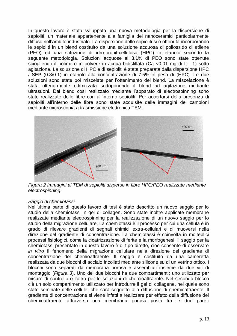
In questo lavoro è stata sviluppata una nuova metodologia per la dispersione di sepioliti, un materiale appartenente alla famiglia dei nanoceramici particolarmente diffuso nell‟ambito industriale. La dispersione delle sepioliti si è ottenuta incorporando le sepioliti in un blend costituito da una soluzione acquosa di poliossido di etilene (PEO) ed una soluzione di idro-propil-cellulosa (HPC) in etanolo secondo la seguente metodologia. Soluzioni acquose al 3.1% di PEO sono state ottenute sciogliendo il polimero in polvere in acqua bidistillata (Ca <0,01 mg di lt - 1) sotto agitazione. La soluzione di HPC e di sepioliti è stata preparata dalla dispersione HPC / SEP (0.8/0.1) in etanolo alla concentrazione di 7,5% in peso di (HPC). Le due soluzioni sono state poi miscelate per l‟ottenimento del blend. La miscelazione è stata ulteriormente ottimizzata sottoponendo il blend ad agitazione mediante ultrasuoni. Dal blend così realizzato mediante l‟apparato di electrospinning sono state realizzate delle fibre con all‟interno sepioliti. Per accertarsi della presenza di sepioliti all‟interno delle fibre sono state acquisite delle immagini dei campioni mediante microscopia a trasmissione elettronica TEM.

Figura 2 Immagini al TEM di sepioliti disperse in fibre HPC/PEO realizzate mediante electrospinning.

Saggio di chemiotassi Nell‟ultima parte di questo lavoro di tesi è stato descritto un nuovo saggio per lo studio della chemiotassi in gel di collagen. Sono state inoltre applicate membrane realizzate mediante electrospinning per la realizzazione di un nuovo saggio per lo studio della migrazione cellulare. La chemiotassi è il processo per cui una cellula è in grado di rilevare gradienti di segnali chimici extra-cellulari e di muoversi nella direzione del gradiente di concentrazione. La chemiotassi è coinvolta in molteplici processi fisiologici, come la cicatrizzazione di ferite e la morfogenesi. Il saggio per la chemiotassi presentato in questo lavoro è di tipo diretto, cioè consente di osservare in vitro il fenomeno della migrazione cellulare nella direzione del gradiente di concentrazione del chemioattraente. Il saggio è costituito da una cameretta realizzata da due blocchi di acciaio incollati mediante silicone su di un vetrino ottico. I blocchi sono separati da membrana porosa e assemblati insieme da due viti di montaggio (Figura 3). Uno dei due blocchi ha due compartimenti; uno utilizzato per misure di controllo e l‟altro per le soluzioni di chemioattraente. Nel secondo blocco c'è un solo compartimento utilizzato per introdurre il gel di collagene, nel quale sono state seminate delle cellule, che sarà soggetto alla diffusione di chemioattraente. Il gradiente di concentrazione si viene infatti a realizzare per effetto della diffusione del chemioattraente attraverso una membrana porosa posta tra le due pareti

200 nm

200 nm

400 nm 200 nm

p. 14

comunicanti dei due blocchi precedentemente descritti. Il processo di diffusione è stato studiato mediante microscopia in fluorescenza, mediante la quale sono state realizzate opportune curve di calibrazione e determinati i coefficienti di diffusione. Il moto delle cellule sotto l‟azione del chemioattraente è stato monitorato mediante microscopia “time lapse”. L‟analisi off-line delle immagini ha permesso di ricostruire la traiettoria descritta delle cellule, e di valutarne la risposta al gradiente di concentrazione principalmente in termini di indice chemotattico (Figura 3b). L‟indice chemotattico (I) permette di valutare quantitativamente i movimenti cellulari. Esso è un indicatore della direzionalità delle traiettorie verso la fonte di chemoattraente ed è compreso tra 0 (movimento random) ed 1 (movimento totalmente direzionale). Per tempi di osservazione sufficientemente lunghi, l‟indice chemotattico per la singola cellula (Im) è definito come il rapporto tra lo spostamento netto nella direzione del gradiente (Yt) e la lunghezza totale del percorso (Lt). Un ulteriore parametro caratteristico della migrazione cellulare è la polarizzazione della cellula, che. è stata quantificata in termini del rapporto tra asse maggiore e minore passante per il centroide della cellula.

time [min]

50 100 150 200 250 300

Chem

ota

ctic index

-0,10

-0,05

0,00

0,05

0,10

0,15

0,20

25

28

22 16

27

(4)(10)

(7)

(5)

(2)

a b

Figura 3 a) Immagine della cella di chemiotassi. b) Indice chemotattico in funzione del tempo in un esperimento con cellule Jurkat in gel di collagene. In questo lavoro, sono stati condotti esperimenti su tre diverse linee cellulari al fine di osservarne la risposta ad un gradiente di concentrazione di chemoattraente. E‟ stato altresì analizzato il comportamento delle cellule in assenza di stimoli migratori esterni mediante prove di controllo.

Saggio di migrazione transepiteliale Anche la camera di migrazione transepiteliale è costituita da due compartimenti nei quali le cellule possono essere indotte a migrare attraverso una membrana porosa, in questo caso da un compartimento superiore realizzata mediante electrospinning ad un compartimento inferiore nel quale è presente una soluzione di chemoattraente. Nello specifico il compartimento superiore è costituito da un cestello sul quale viene realizzata una membrana mediante electrospinning esponendo la superfice interessata del cestello direttamente al getto polimerico. Il cestello può essere introdotto in una normale piastra multiwell da laboratorio lasciando libera un‟intercapedine sul fondo, che viene così a realizzare il secondo compartimento.

p. 15

Al fine di realizzare un saggio di migrazione transepiteliale sulla membrana del cestello vengono seminate delle cellule di tipo CACO-2 coltivate seguendo metodologie standard per colture cellulari. Le cellule a confluenza danno luogo alla formazione di un monolayer osservato mediante microscopia ottica in contrasto di fase (Figura 4). Il saggio si realizza seminando all‟interno del cestello (comparto superiore) le cellule di cui si vuole osservare la migrazione cellulare in opportuno terreno di coltura. Nel comparto inferiore viene introdotta la soluzione di chemoattraente.

Figura 4 Immagini in contrasto di fase di cellule CACO-2 su membrana di PLA realizzata mediante electrospinning.

p. 16

Chapter 1 STATE OF THE ART OF THE ELECTROSPINNING PROCESS

1 Introduction

In the second half of the 20th century, the use of polymers in our daily life has grown tremendously. Polymers are used in different forms and for a wide range of applications. Noticeable among these are the synthetic and regenerated polymers that have found applications not only in the textile and apparel sector but also in many industrial usages like tire cords, reinforcing and structural agents, barrier films, food and packaging products, automotive parts, etc. The process of making fibers from polymers generally involves spinning, wherein the polymer is extruded through a spinneret to form fibers under suitable shear rates and temperatures. This conventional fiber formation process is generally followed by drawing, which involves the plastic stretching of the as-spun material to increase its strength and modulus. Depending on whether the polymer is in the molten state or in solution, the process is likewise termed as melt-spinning or solution spinning, respectively. Typical average diameters obtained by these conventional spinning methods are about 10 μm and higher. Over the last ten years, a novel technique has been re-explored to generate polymeric fibers in the submicron range. This technique, termed as electrospinning, produces filaments that are in a diameter range one or two orders of magnitude smaller than those obtained from the conventional melt-spinning and solution-spinning processes. Electrospinning is, therefore, a unique process because it can generate submicron polymeric fibers. Electrospun fibers can have a diameter as low as 50 - 100 nm. The potential of these electrospun nanofibers in human healthcare applications is promising, for example in tissue/organ repair and regeneration, as a vectors to deliver drugs and therapeutics, as biocompatible and biodegradable medical implant devices, in medical diagnostics instrumentation, as protective fabrics against environmental and infectious agents in hospitals and general surroundings, and in cosmetic and dental applications.

Tissue/organ repair and regeneration are new avenues for potential treatment, circumventing the need for donor tissues and organs in transplantation and reconstructive surgery. In this approach, a scaffold is usually required, which can be fabricated from either natural or synthetic polymers by many processing techniques, including electrospinning and phase separation. The biocompatibility of the scaffold is usually tested ex vivo by culturing organ-specific cells on the scaffold and monitoring cell growth and proliferation. An animal model is used to study the biocompatibil ity of the scaffold in a biological system before the scaffold is introduced into patients for tissue-regeneration applications. Nanofiber scaffolds are well suited to tissue engineering as they can be fabricated and shaped to fill anatomical defects; its architecture can be designed to provide the mechanical properties necessary to support cell growth, proliferation, differentiation, and motility; and it can be engineered to provide growth factors, drugs, therapeutics, and genes to stimulate tissue regeneration. An inherent property of nanofibers is that they mimic the extracellular matrices (ECM) of tissues and organs. The ECM is a complex composite of fibrous proteins such as collagen and fibronectin, glycoproteins, proteoglycans, soluble proteins such as growth factors, and other bioactive

p. 17

molecules that support cell adhesion and growth. Studies of cell-nanofiber interactions have shown that cells adhere and proliferate well when cultured on polymer nanofibers[1-3]. In another system[4,5], a drug-bound, pH-responsive polymer is targeted to diseased cells through cell receptor binding of a ligand. The polymer is subsequently endocytosed into the endosomal compartment of the cells. In the low pH environment of the endosome, the polymer backbone separates from the drug, destabilizes the endosomal membrane, and releases the drug into the cytoplasmic compartment of the cells. This system of drug delivery can also be used to deliver therapeutics, silencing RNA, antisense oligonucleotides, and vaccines to specific cell types, targeting specific compartments and organelles.

High porosity, interconnectivity, microscale interstitial space, and a large surface-to-volume ratio make nonwoven electrospun nanofiber meshes an excellent material for membrane preparation, especially in biotechnology and environmental engineering applications. Ligand molecules, biomacromolecules, or even cells can be attached or hybridized with the nanofiber membrane for applications in protein purification and waste water treatment (affinity membranes), enzymatic catalysis or synthesis (membrane bioreactors), and, in the future, chemical analysis and diagnostics (biosensors). Electrospun nanofibers can form an effective size exclusion membrane for particulate removal from wastewater. Particle removal from air by a nanofiber membrane has been studied by Gibson et al.[6]. The nanofiber membrane shows an extremely effective removal (~100% rejection) of airborne particles with diameters between 1 μm and 5 μm by both physical trapping and adsorption. For particle removal from aqueous solution, recent results show that electrospun membranes can successfully remove particles 3-10 μm in size (>95 %) rejection) without a significant drop in flux performance[7]. No particles were found trapped in the membrane, so the membrane could be effectively recovered upon cleaning. This opens up new avenues of application of electrospun membranes for the pre-treatment of water prior to reverse osmosis.

2 Historical Background

The origin of electrospinning as a viable fiber spinning technique can be traced back to the early 1930s. In 1934, Formhals patented his first invention relating to the process and the apparatus for producing artificial filaments using electric charges[8]. Though the method of producing artificial threads using an electric field had been experimented with for a long time, it had not gained importance until Formhals‟s invention due to some technical difficulties in earlier spinning methods, such as fiber drying and collection. Formhals‟s spinning process consists of a movable thread collecting device to collect the threads in a stretched condition, like that of a spinning drum in the conventional spinning. Formhals‟s process was capable of producing threads aligned parallel on to the receiving device in such a way that it can be unwound continuously. In his first patent, Formhals reported the spinning of cellulose acetate fibers using acetone as the solvent. The first spinning method adopted by Formhals had some technical disadvantages. It was difficult to completely dry the fibers after spinning due to the short distance between the spinning and collection zones, which resulted in a less aggregated web structure. In a subsequent patent, Formhals refined his earlier approach to overcome the aforementioned drawbacks[9]. In the refined process, the distance between the feeding nozzle and the fiber collecting device was altered to give more drying time for the electrospun fibers. In

p. 18

1940, Formhals patented another method for producing composite fiber webs from multiple polymer and fiber substrates by electrostatically spinning polymer fibers on a moving base substrate[10].

In the 1960s, fundamental studies on the jet forming process were initiated by Taylor [11]. In 1969, Taylor studied the shape of the polymer droplet produced at the tip of the needle when an electric field is applied and showed that it is a cone and the jets are ejected from the the cone apex[11]. The shape of the jet was later referred to by other researchers as the “Taylor Cone” in subsequent literature. By a detailed examination of different viscous fluids, Taylor determined that an angle of 49.3 degrees is required to balance the surface tension of the polymer with the electrostatic forces. The conical shape of the jet is important because it defines the onset of the extensional velocity gradients in the fiber forming process[12].

In subsequent years, focus shifted to studying the structural morphology of nanofibers. Researchers worked on the structural characterization of fibers and the understanding of the relationships between the structural features and process parameters. Wide-angle X-ray diffraction (WAXD), scanning electron microscopy (SEM), transmission electron microscopy (TEM), and differential scanning calorimetry (DSC) have been used to characterize electrospun nanofibers. In 1971, Baumgarten reported the electrospinning of acrylic microfibers with diameter ranging from 500 to 1100 nm[13]. Baumgarten determined the spinnability limits of a polyacrylonitrile/dimethylformamide (PAN/DMF) solution and observed a specific dependence of fiber diameter on the viscosity of the solution. He showed that the diameter of the jet reached a minimum value after an initial increase in the applied field and then became larger with increasing electric fields. Larrondo and Mandley produced polyethylene and polypropylene fibers from the melt, which were found to be relatively larger in diameter than solvent spun fibers[14,15]. They studied the relationship between the fiber diameter and melt temperature and showed that the diameter decrease with increasing melt temperature. Furthermore, fiber diameter reduced by 50% when the applied voltage doubled, thus showing the significance of applied voltage on fiber size. In 1987, Hayati et al. studied the effects of electric field, experimental conditions, and the factors affecting fiber stability and atomization. They concluded that liquid conductivity plays a major role in the electrostatic disruption of liquid surfaces. Results showed that highly conducting fluids with increasing applied voltage produced highly unstable streams that whipped around in different directions. Relatively stable jets were produced with semi conducting and insulating liquids, such as paraffinic oil[16]. Their results also showed that unstable jets produce fibers with broader diameter distribution.

After a hiatus of a decade or so, a major upsurge in research on electrospinning took place due to increased knowledge on the potential applications of nanofibers in different areas, such as high efficiency filter media, protective clothing, catalyst substrates, and adsorbent materials. Research on nanofibers gained momentum due to the work of Doshi and Reneker[16], who studied the structure of polyethylene oxide (PEO) nanofibers by varying solution concentration and applied electric potential [17]. Jet diameters were measured as a function of distance from the apex of the cone, and they observed that the jet diameter decreases with increasing distance. They found that PEO solutions with viscosity less than 800 centipoise (cP) were too dilute to form a stable jet and solutions with viscosity more than 4000 cP were too thick to form fibers. Jaeger et al. studied the thinning of fibers as the extrusion progressed in PEO/water electrospun fibers and observed that the diameter of the flowing jet

p. 19

decreased to 19 µm in traveling 1 cm from the orifice, 11 µm after traveling 2 cm, and 9 µm after 3.5 cm[18]. Their experiment showed that solutions with conductivities in the range of 1000–1500 µs.cm-1 heated up the jet due to the electric current in the order of 1–3 µA.

Electrospun fibers often present on the surface bulges called beads. The electrospun beaded fibers are related to the instability of the jet from the polymer solution. In 1962, Deitzel et al. showed that an increase in the applied voltage changes the shape of the surface from which the jet originates and the shape change has been correlated to an increase of bead defects[19]. They tried to control the deposition of fibers by using a multiple field electrospinning apparatus that provided an additional field of similar polarity on the jets[20]. Warner et al.[21] and Moses et al.[22,23] pursued a rigorous work on the experimental characterization and evaluation of fluid instabilities, which are crucial for the understanding of the electrospinning process. Shin et al. designed a new apparatus that could give enough control over the experimental parameters to quantify the electrohydrodynamics of the process[24]. Spivak and Dzenis showed that the Ostwalt–de Waele power law could be applied to the electrospinning process[25]. Gibson et al. studied the transport properties of electrospun fiber mats, and they concluded that nanofiber layers give very less resistance to the moisture vapor diffusional transport[26].

In conclusion, the process of electrospinning is suitable to many kind of applications, some of which are still being explored. An example is the use of electrospinning to fabricate new biopolymer scaffolds for in vitro assays or tissue engineering applications. The technique of electrospinning could be also used in order to improve the dispersion of nanoparticles.

3 Electrospinning Theory and Process

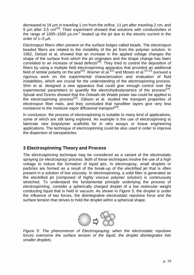
The electrospinning technique may be considered as a variant of the electrostatic spraying (or electrospray) process. Both of these techniques involve the use of a high voltage to induce the formation of liquid jets. In electrospray, small droplets or particles are formed as a result of the break-up of the electrified jet that is often present in a solution of low viscosity. In electrospinning, a solid fiber is generated as the electrified jet (composed of highly viscous polymer solution) is continuously stretched. To understand the fundamental principle underlying the process of electrospinning, consider a spherically charged droplet of a low molecular weight conducting liquid that is held in vacuum. As shown in Figure 5, the droplet is under the influence of two forces, the disintegrative electrostatic repulsive force and the surface tension that strives to hold the droplet within a spherical shape.

Figure 5: The phenomenon of Electrospraying: when the electrostatic repulsive forces overcome the surface tension of the liquid, the droplet disintegrates into smaller droplets.

p. 20

At equilibrium, the two forces completely balance each other, and this is expressed by the following equation:

02

2

0

28

1

R

R

Q (1.1)

where Q is the electrostatic charge on the surface of the droplet, R is the radius of the droplet, εo is the dielectric permeability of vacuum and σ0 is the surface tension coefficient. With increasing electric field strength, the charge on the surface of the droplet increases until it reaches a critical point where the electrostatic repulsive force overcomes the surface tension. When this happens the droplet disintegrates leading to the formation of smaller droplets (see Figure 5). This process is termed as electrospraying and has been utilized extensively for automotive spray painting.

If this concept is extended to a high molecular weight polymer solution that has sufficient chain entanglements, then instead of the formation of the droplets, a steady jet is formed that later solidifies in a polymer filament. Thus, the fundamental principle underlying fiber formation by electrospinning can be stated as follows: a high electric potential is applied to a polymer solution (or melt) suspended from the end of a spinneret providing an electrostatic charge to the polymer solution. At low electric potentials, the disintegrative electrostatic repulsive forces that primarily reside on the liquid surface are balanced by the surface tension. At high electric potentials, the electrostatic repulsive force at the surface of the fluid overcomes the surface tension and this results in the ejection of a charged jet. The jet extends along a straight line for a certain distance, and then bends and follows a looping and spiraling path. The electrostatic repulsion forces can elongate the jet to several thousand times leading to the formation of a very thin jet (Jet Initiation). When the solvent evaporates, solidified polymer filaments are collected on a grounded target in the form of a non-woven fabric (Bending Instability). The small diameter provides a large surface to volume ratio that makes these electrospun fabrics interesting candidates for a number of applications.

Electrospinning: Jet Initiation

The behavior of electrically driven jets, the shape of the jet originating surface, and the jet instability are some of the critical areas in the electrospinning process that require further research. Rayleigh[27] and Zeleny[28] gave initial insight into the study of the behaviour of liquid jets, later followed by Taylor[11]. Taylor showed that a conical shaped surface with an angle of 49.3°, referred to as the Taylor cone, is formed when a critical potential is reached to disturb the equilibrium of the droplet at the tip of the capillary, that is, the initiating surface. When a high potential is applied to the solution, electrical forces and surface tension help in creating a protrusion wherein the charges accumulate. The high charge per unit area at the protrusion pulls the solution further to form a conical shape, which on further increase in the potential initiates the electrospinning process by jetting. Yarin and coworkers[29] studied the formation of a conical meniscus (already referred to as the Taylor Cone) and the phenomena of jetting from liquid droplets in electrospinning of nanofibers. It was concluded that the critical half angle of the conical meniscus of the charged fluid does not depend on the fluid properties for Newtonian fluids, since an increase in surface tension was always accompanied by an increase in the critical electric field. It

p. 21

was shown both theoretically and experimentally, that as a liquid surface develops a critical shape; its configuration approached the shape of a cone with a half angle of 33.5o rather than a Taylor cone of 49.3o. In elastic or unrelaxed viscoelastic fluids, the geometrical sharpness of the critical hyperboloid was found to depend on both elastic and surface tension forces.

4 Bending instability

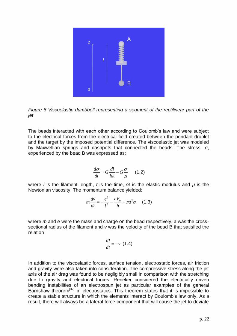
The jet ejected from the apex of the cone continues to thin down along the path of its travel towards the collector, and the jetting mode has been termed as electrohydrodynamic cone-jet[30]. The charges in the jet accelerate the polymer solution in the direction of the electric field towards the collector, thereby closing the electrical circuit. While moving towards the collector the jet undergoes a chaotic motion or bending instability as suggested by Yarin et al. due to the repulsive forces originating from the charged ions within the electrospinning jet[29]. The bending instability was originally thought to be occurring by a single jet splitting into multiple thin fiber filaments due to radial charge repulsion, which was termed as splaying[17]. Doshi and Reneker argued that as the fiber diameter decreases due to the simultaneous stretching of the jet and the evaporation of the solvent, the increased charge density splits the jet into smaller jets. This splitting is expected to occur repeatedly, resulting in smaller diameter fibers. However, recent observations suggest that the rapid growth of a non-axisymmetric or whipping instability causes the stretching and bending of the jets[32]. Warner et al. and Shin et al. have used high-speed photography (with exposure times down to 1 ms) to confirm that the unstable region of the jet, which appears as an inverted cone suggesting multiple splitting, is actually a single rapidly whipping jet[21,24]. They suggest that the whipping phenomena occur so fast that the jet appears to be splitting into smaller fiber jets, resulting in ultra fine fibers. A steady state model of the jets using nonlinear power law constitutive equations (Oswald–de Waele model[33,34]) was developed by Spivak et al.[35]. Reneker and his coworkers have contributed significantly to the study of the instability behavior and developed a mathematical viscoelastic model for the rectilinear electrified jet. Reneker et al.[36] proposed the following mechanism for the onset of jet instability: upon initiation, the jet of the polymer solution was rapidly accelerated away from the capillary end toward the target by electrostatic forces. This provided a longitudinal stress that stabilized the jet, keeping it initially straight. At some distance from the point of initiation, the jet of the polymer solution started to undergo stress relaxation. The point along the jet at which this occurred depended on the electric field strength. Increasing the electric field strength increased the length of the stable jet. Once stress relaxation began, the electrostatic interaction between the charged elements of the jet began to dominate the ensuing motion, initiating and perpetuating the chaotic motion of the jet. A mathematical model was proposed to describe the chaotic motion of the jet, also referred to as the „bending instability‟ or „whipping‟ of the jet. The bending instabilities in electrospun jets were modeled as a system of connected viscoelastic dumbbells. In

Figure 6, the beads, „A‟ and „B‟, at the end of the dumbbell were characterized by appropriate mass and charge.

p. 22

Figure 6 Viscoelastic dumbbell representing a segment of the rectilinear part of the jet

The beads interacted with each other according to Coulomb‟s law and were subject to the electrical forces from the electrical field created between the pendant droplet and the target by the imposed potential difference. The viscoelastic jet was modeled by Maxwellian springs and dashpots that connected the beads. The stress, ζ, experienced by the bead B was expressed as:

G

ldt

dlG

dt

d (1.2)

where l is the filament length, t is the time, G is the elastic modulus and μ is the Newtonian viscosity. The momentum balance yielded:

20

2

2

ah

eV

l

e

dt

dvm (1.3)

where m and e were the mass and charge on the bead respectively, a was the cross-sectional radius of the filament and v was the velocity of the bead B that satisfied the relation

vdt

dl (1.4)

In addition to the viscoelastic forces, surface tension, electrostatic forces, air friction and gravity were also taken into consideration. The compressive stress along the jet axis of the air drag was found to be negligibly small in comparison with the stretching due to gravity and electrical forces. Reneker considered the electrically driven bending instabilities of an electrospun jet as particular examples of the general Earnshaw theorem[37] in electrostatics. This theorem states that it is impossible to create a stable structure in which the elements interact by Coulomb‟s law only. As a result, there will always be a lateral force component that will cause the jet to deviate

p. 23

from its original initiated path into a looping spiraling trajectory. To better understand the Earnshaw instability relevant to the electrospinning context, three point-like charges, originally in a straight line were considered by Reneker and coworkers[36]. As shown in Figure 7, these point-like charges at A, B and C carried the same charge

e. Two Coulomb forces having magnitudes 2

2

r

eF pushed against charge B from

opposite directions. If a perturbation caused the point B to move off the line by a distance δ to B‟, a net force

3

2

1 2cos2r

eFF (1.5)

acted on the charge B in a direction perpendicular to the line, and tended to cause B to move further in the direction of the perturbation away from the line between the fixed charges, A and C. In the linear approximation the growth of the small bending perturbation that was characterized by δ is expressed by:

3

1

2

2

2 2

l

e

dt

dm (1.6)

where m was the mass and l1 was the distance between the charges A and B, as shown in Figure 7. The solution of this equation,

t

ml

e 2

1

3

1

2

0

2exp (1.7)

showed that small perturbations increased exponentially. The increase was

sustained because the electrostatic potential energy of the system decreased as r

e 2

when the perturbations grew. This mechanism was believed to be responsible for the observed bending instability of jets in electrospinning. The electrospun jet was visualized as a series

Figure 7 Illustration of the Earnshaw instability leading to bending of an electrified jet.[36]

p. 24

of charged beads, such that the equation governing the radius vector of the position

of the ith bead was: iiii kzjyixr

iii

ii

iav

ii

ui

uiui

JNi

ji

ij

i

ysignyjxsignxi

yx

ka

rrl

ak

h

Verr

R

e

dt

rdm

2

122

2

1

2

1;,1

0

3

2

2

2

(1.8)

where 21

222

jijijiij zzyyxxR , h was the distance from pendant drop

to the collector, Vo was the potential drop, aui was the filament radius at the ith bead, α was the surface tension coefficient and ζui was the stress acting in the ith bead. Both space and time dependant perturbations lead to the development of an electrically driven instability. Small perturbations modeled as

tLy

tLx

i

i

cos10

sin10

3

3

(1.9)

where ω was the perturbation frequency, were introduced by Reneker and coworkers[36] in the final analysis to obtain the trajectories of the jet. The three-dimensional equations of the dynamics of the electrospun jets were then solved numerically for jet path and trajectory. The predicted jet path and trajectory were compared to experimental results obtained for a 6wt% PEO solution in 60/40 water/ethanol electrospun at a field strength of 1kV/cm. The predicted motion of the jet was in good agreement with the experimental data until about 2-3 ms after jet initiation. After 3 ms, the predicted motion deviated from the experimentally observed results. The jet velocity was predicted to be a bit larger (1-2 m/s) than the experimentally observed value of 0.8-1.1 m/s in the first 8 ms after jet initiation. The predicted lateral motion and the lateral velocity of the jet were at least two orders of magnitude higher than the experimentally observed results. Warner et al.[38] measured the average jet velocity to be 15 m/s in their experiments involving electrospinning of 2 wt% aqueous PEO solution. Based on the area reduction calculations, the draw ratio of the jet was estimated to be about 60,000 taking into account the evaporation of the solvent[36]. The longitudinal strain rate was calculated to be about 105 s-1. In a previous paper, Lorrondo and Manley[14] determined the strain rate to be of the order of 50 s-1 and earlier works of Doshi and Reneker[17] have reported strain rates as high as 104 s-1.

From the above discussion it is apparent that electrostatic interactions between individual charge elements in the jet and between charge elements and the macroscopic electric field are primarily responsible for initiation and perpetuation of the bending instability. Keeping this in mind, Deitzel et al.[20] designed an

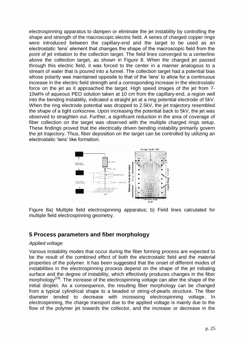
p. 25

electrospinning apparatus to dampen or eliminate the jet instability by controlling the shape and strength of the macroscopic electric field. A series of charged copper rings were introduced between the capillary-end and the target to be used as an electrostatic „lens‟ element that changes the shape of the macroscopic field from the point of jet initiation to the collection target. The field lines converged to a centerline above the collection target, as shown in Figure 8. When the charged jet passed through this electric field, it was forced to the center in a manner analogous to a stream of water that is poured into a funnel. The collection target had a potential bias whose polarity was maintained opposite to that of the „lens‟ to allow for a continuous increase in the electric field strength and a corresponding increase in the electrostatic force on the jet as it approached the target. High speed images of the jet from 7-10wt% of aqueous PEO solution taken at 10 cm from the capillary-end, a region well into the bending instability, indicated a straight jet at a ring potential electrode of 5kV. When the ring electrode potential was dropped to 2.5kV, the jet trajectory resembled the shape of a tight corkscrew. Upon increasing the potential back to 5kV, the jet was observed to straighten out. Further, a significant reduction in the area of coverage of fiber collection on the target was observed with the multiple charged rings setup. These findings proved that the electrically driven bending instability primarily govern the jet trajectory. Thus, fiber deposition on the target can be controlled by utilizing an electrostatic „lens‟ like formation.

Figure 8a) Multiple field electrospinning apparatus; b) Field lines calculated for multiple field electrospinning geometry.

5 Process parameters and fiber morphology

Applied voltage

Various instability modes that occur during the fiber forming process are expected to be the result of the combined effect of both the electrostatic field and the material properties of the polymer. It has been suggested that the onset of different modes of instabilities in the electrospinning process depend on the shape of the jet initiating surface and the degree of instability, which effectively produces changes in the fiber morphology[19]. The increase of the electrospinning voltage can alter the shape of the initial droplet. As a consequence, the resulting fiber morphology can be changed from a typical cylindrical shape to a beaded or string-of-pearls structure. The fiber diameter tended to decrease with increasing electrospinning voltage. In electrospinning, the charge transport due to the applied voltage is mainly due to the flow of the polymer jet towards the collector, and the increase or decrease in the

p. 26

current is attributed to the mass flow of the polymer from the nozzle tip. Deitzel et al. have inferred that the change in the spinning current is related to the change in the instability mode[19]. They experimentally showed that an increase in applied voltage causes a change in the shape of the jet initiating point, and hence in the structure and morphology of the fibers. Experiments on a PEO/water system have shown an increase in the spinning current with an increase in the applied voltage[19]. It was also observed that for the PEO/water system, the fiber morphology changed from a defect free fiber at an initiating voltage of 5.5KV to a highly beaded structure at a voltage of 9.0KV[14]. The occurrence of beaded morphology has been correlated to a steep increase in the spinning current, which controls the bead formation in the electrospinning process. Beaded structure reduces the surface area, which ultimately influences the filtration abilities of nanofibers.

Earlier in 1971, Baumgarten while carrying out experiments with acrylic fibers observed an increase in fiber length of approximately twice and small changes in fiber diameter with an increase in applied voltage. Megelski et al. investigated the voltage dependence on the fiber diameter using polystyrene (PS). The PS fiber size decreased from about 20 µm to 10 µm with an increase in voltage from 5KV to 12KV, while there was no significant change observed in the pore size distribution[39]. These results are in line with the interpretation of Buchko et al.[12], who observed a decrease in fiber diameter with an increase in the applied field while spinning silk like polymer fibers with fibronectin functionality (SLPF). It is generally accepted that an increase in the applied voltage increases the deposition rate due to higher mass flow from the needle tip. Jaeger et al. used a two-electrode setup for electrospinning by introducing a ring electrode in between the nozzle and the collector[18]. The ring electrode was set at the same potential as the electrode immersed in the polymer solution. This setup was thought to produce a field-free space at the nozzle tip to avoid changes in the shape of the jet initiating surface due to non uniform potential[18]. Although this setup reduces the unstable jet behavior at the initiation stage, bending instability is still dominant at later stages of the process, causing an uneven chaotic motion of the jet before depositing itself as a nonwoven matrix on the collector.

Nozzle collector distance

The structure and morphology of electrospun fibers is easily affected by the nozzle to collector distance because of their dependence on the deposition time, evaporation rate, and whipping or instability interval. Buchko et al. examined the morphological changes in SLPF and nylon electrospun fibers with variations in the distance between the nozzle and the collector screen. They showed that regardless of the concentration of the solution, a shorter nozzle-collector distance produces wet fibers and beaded structures. SLPF fiber morphology changed from round to flat shape with a decrease in the nozzle collector distance from 2 cm to 0.5 cm. This result shows the effect of the nozzle collector distance on fiber morphology. The work also showed that aqueous polymer solutions require more distance for dry fiber formation than systems that use highly volatile organic solvents. Megelski et al. observed bead formation in electrospun PS fibers on reducing the nozzle to collector distance, while the ribbon shaped morphology was preserved with a decrease in the nozzle to collector distance[39].

p. 27

Polymer flow rate

The flow rate of the polymer from the syringe is an important process parameter as it influences the jet velocity and the material transfer rate. In the case of PS fibers, Megelski et al. observed that the fiber diameter and the pore diameter increased with an increase in the polymer flow rate[55]. As the flow rate increased, fibers had pronounced beaded morphologies and the mean pore size increased from 90 to 150 nm[55].

Spinning environment

Environmental conditions around the spinneret, like the surrounding air, its relative humidity (RH), vacuum conditions, surrounding gas, etc., influence the fiber structure and morphology of electrospun fibers. Baumgarten observed that acrylic fibers spun in an atmosphere of more than 60% relative humidity do not dry properly and get entangled on the surface of the collector[13]. The breakdown voltage of the atmospheric gases is said to influence the charge retaining capacity of the fibers[13]. Srinivasarao et al. proposed a new mechanism for pore formation by evaporative cooling called “breathe figures”[56]. Breathe figures occur on the fiber surfaces due to the imprints of condensed moisture droplets caused by the evaporative cooling of moisture in the air surrounding the spinneret. Megelski et al. investigated the pore geometry of PS fibers at varied RH and emphasized the importance of phase separation mechanisms in explaining the pore formation of electrospun fibers[39].

6 Solution parameters and fiber morphology

Solution concentration

Solution concentration sets the limiting boundaries for the formation of electrospun fibers due to variations in the viscosity and surface tension[14]. A low concentration solution forms droplets due to the influence of surface tension, while higher concentrations inhibit fiber formation due to higher viscosity. Previously published literature has documented the difficulties in the electrospinning of polymers like PEO,[19] PAN,[20] and PDLA[42] at certain concentration levels. By increasing the concentration of polystyrene solution, the fiber diameter increased and the pore size reduced to a narrow distribution[39]. In the case of a PEO/water system, a bimodal distribution in fiber diameter was observed at higher concentrations[19]. In the PEO system, Dietzel et al. related the average fiber diameter and the solution concentration by a power law relationship[20]. Dietzel et al. interpreted the variations in fiber diameter and morphology to the shape of the jet-originating surface, which is in line with the observations of Zong et al.[41]. Undulating morphologies in fibers were attributed to the delayed drying and the stress relaxation behavior of the fibers at lower concentrations[41]. It can be concluded that the concentration of the polymer solution influences fiber spinning and controls fiber structure and morphology.

Solution conductivity

Polymers are mostly conductive, with a few exceptions of dielectric materials, and the charged ions in the polymer solution are highly influential in jet formation. The ions increase the charge-carrying capacity of the jet, thereby subjecting it to higher

p. 28

tension with the applied electric field. Baumgarten showed that the jet radius varied inversely as the cube root of the electrical conductivity of the solution[13]. Zong et al. demonstrated the effect of ions by adding ionic salt on the morphology and diameter of electrospun fibers[41]. They found that PDLA fibers with the addition of ionic salts like KH2PO4, NaH2PO4, and NaCl produced beadless fibers with relatively smaller diameters ranging from 200 to 1000 nm[41].

Volatility of solvent

As electrospinning involves rapid solvent evaporation and phase separations due to jet thinning, solvent vapor pressure critically determines the evaporation rate and the drying time. Solvent volatility plays a major role in the formation of nanostructures by influencing the phase separation process. Bognitzki et al. found that the use of highly volatile solvents like dichloromethane yielded PLLA fibers with pore sizes of 100 nm in width and 250 nm in length along the fiber axis[43]. Lee et al. evaluated the effect of volume ratio of the solvent on the fiber diameter and morphology of electrospun PVC fibers[45]. Average fiber diameters decreased with an increase in the amount of DMF in the THF/DMF mixed solvent. Lee et al. found the electrolytic nature of the solvent to be an important parameter in electrospinning[44]. Megelski et al. studied the structure of electrospun fibers with respect to the physical properties of solvents. The influence of vapor pressure was evident when PS fibers spun with different THF/DMF combinations resulted in micro and nanostructure morphologies at higher solvent volatility and a much-diminished microstructure at lower solvent volatility[39].

7 Aim of this thesis

This work can be divided in four parts. In the first part, based on a review of literature an apparatus of electrospinning was developed with the aim of processing biopolymer solutions. The setup of the apparatus was initially tested by using model polymer solutions. The apparatus was then tested on biopolymer solutions widely described in the literature and different configurations were designed in order to obtain cylindrical and aligned fiber scaffolds. In the second part, a procedure to fabricate nano/micro fibrous scaffolds of an ester of hyaluronic acid (HYAFF-11) by electrospinning was implemented. The effects of solution properties and processing parameters on the structure and morphology of the HYAFF-11 electrospun membranes were thoroughly investigated to find the optimal processing conditions. The morphology of electrospun polymer fibers is known to depend on the strength of the electric field and on the solution viscosity (e.g. concentration). In particular, it is expected that higher solution concentrations favour the formation of uniform nanofibers with no bead-like defects. Furthermore, the diameter of the nanofibers decreases with electrospinning voltage. We have also studied cell proliferation on electrospun HYAFF-11 scaffolds in comparison with electrospun PLA and PCL scaffolds. In the third part of the thesis the electrospinning process was used to fabricate polymer nanofibers containing one-dimensional arrays of SEP nanoparticles. A blend obtained by mixing solution of PEO with solution of HPC was used as a template to arrange the SEP nanoparticles within the fibers during electrospinning. In the last part of this thesis we present a novel assay for chemotaxis in a direct-viewing chamber and show how electrospun scaffolds could be use to improve the chemotaxis assay and to study cell migration. In the

p. 29

chemotaxis assay presented in this work a chemoattractant concentration gradient in a collagen gel seeded with cells is generated by diffusion through a porous membrane. The diffusion process is monitored by fluorescence microscopy of FITC-labelled dextran. Cell motion under the action of the chemoattractant gradient is followed by time-lapse video microscopy. Cell tracking is performed off-line by image analysis and the results are expressed in terms of a chemotactic index.

p. 30

Chapter 2 Materials and Methods

1 Experimental apparatus

Electrospinning is a process by which a polymer solution or melt can be spun into smaller diameter fibers using a high potential electric field. This generic description is appropriate as it covers a wide range of fibers with submicron diameters that are normally produced by electrospinning. Based on earlier research results, it is evident that the average diameter of electrospun fibers ranges from 100 nm–500 nm. In textile and fiber science related scientific literature, fibers with diameters in the range 100 nm–500 nm are generally referred to as nanofibers. The advantages of the electrospinning process are its technical simplicity and its easy adaptability. The apparatus used for electrospinning is simple in construction. It consists of a high voltage electric source with positive or negative polarity, a syringe pump with capillaries or tubes to carry the solution from the syringe or pipette to the spinnerette, and a collector made of a conductive material like aluminum. The collector can be made of any shape according to the needs, like a flat plate, rotating drum, etc. A schematic of the electrospinning process is showed in Figure 9. Many previous researchers have used an apparatus similar to the one given in Figure 9 with modifications depending on the process conditions required to spin a wide variety of fine fibers.

Figure 9 Schematic of the electrospinning process.

The polymer solution or melt that has to be spun is forced through a syringe pump to form a pendant drop of the polymer at the tip of the capillary. High voltage potential is applied to the polymer solution inside the syringe through an immersed electrode, thereby inducing free charges into the polymer solution. These charged ions move in

p. 31

response to the applied electric field towards the electrode of opposite polarity, thereby transferring tensile forces to the polymer liquid[45]. At the tip of the capillary, the pendant hemispherical polymer drop takes a cone-like projection in the presence of an electric field. When the applied potential reaches a critical value required to overcome the surface tension of the liquid, a jet of liquid is ejected from the cone tip.

2 Methods to generate oriented electrospun nanofibers

So far, most nanofibers produced by electrospinning are in non-woven form. However, for some application, not only the electrospun nanofiber diameter and their intrinsic properties but also the fiber orientation and the molecular orientation inside nanofibers are relevant, such as in traditional fiber and textile industry. In these cases, electrospun nanofibers should be in either continuous single nanofibers form or uniaxial fiber bundles form, which is a tough target to be achieved, since the polymer jet does not travel in a straight line but in a whipping way during the electrospinning process due to the bending instability. Still, great efforts have been made towards this goal. Until now, there are two basic methods reported in this area.

1. A cylinder collector with high rotating speed.

2. An auxiliary electrode/electrical field.

Researchers have found that by electrospinning nanofibers onto a rotating cylinder collector at a speed up to thousand of rpm (revolution per minute), orientation will be introduced into the so obtained nanofibers. The speed of the rotating cylinder surface should match the alignment speed of the fiber, which is the speed of the solidified jet, in order to achieve a significant orientation. Lower speed or much higher speed are not effective. Figure 11 shows the oriented electrospun nanofibers obtained by this method. From these images and the corresponding statistical analysis of the angle between the long axes of the fibers and their direction (perpendicular to the spin axis of the mandrel), i the degree of alignment of the fibers can be determined. When a rotating steel rod was used to collect the fibres, the electrospinning jet would spread over the length of the rotating bar as shown in Figure 10 along the x-axis. The electrostatic field between the needle tip and the rotating rod does not favour alignment of the electrospun nanofibres. Thus, when aligned fibres are collected just by using a rotating mandrel, a large rotation speed would be needed so that the fibers would quickly be taken up by the rotating mandrel in a circumferential direction. In this case, a rotation speed of 1165 rpm was not fast enough to wind the fibres on the rotating rod to obtain circumferential alignment. However, if the rotation of the mandrel is too fast, it may result in multiple breakages of the collected fiber (Zussman et al 2003a). Li et al (2004).

p. 32

Figure 10 Collecting electrospun fibres on rotating rod with electrospinning jet spreading ower the length of the rod.

a b

Figure 11 Aligned PEO electrospun nanofibers at two different speeds of mandrel a) 400 Hz b) 1400 Hz

Degree

-80 -60 -40 -20 0 20 40 60 80

N/N

(tot)

0,00

0,05

0,10

0,15

0,20

0,25

Degree

-50 0 50

N/N

(tot)

0,0

0,1

0,2

0,3

0,4

0,5

a b

Figure 12 Distribution of the angle between long axis of a fiber and the normal to the spin axis at different mandrel speeds. The results displayed in each plate came from measurements on more then 100 fibers a)400 Hz b)1400Hz.

p. 33

Due to electrostatic interactions too, the nano-fibers were stretched across the gap to form a parallel array, which could be conveniently transferred onto the surface of another substrate for various applications. Figure 13A illustrates the setup used for our electrospinning experiments. It is essentially the same as the conventional configuration except for the use of a collector containing a gap in its middle. Such a collector could be simply fabricated by putting two stripes of electrical conductors (e.g., metals and highly doped silicon) together or by cutting a piece of aluminum foil. The width of the gap could be varied from hundreds of micrometers to several centimeters. Figure 13B shows a cross-sectional view of the electric field strength vectors between the needle and the grounded collector. Unlike the conventional system, the electric field lines in the vicinity of the collector were split into two fractions pointing toward opposite edges of the gap. Figure 13C illustrates the electrostatic forces acting on a charged nanofiber spanning the gap.

Figure 13. (A) Schematic illustration of the setup for electrospinning that was used to generate uniaxially aligned nanofibers. The collector contained two pieces of conductive silicon stripes separated by a gap. (B) Calculated electric field strength vectors in the region between the needle and the collector. The arrows denote the direction of the electrostatic field lines. (C) Electrostatic force analysis of a charged nanofiber spanning across the gap. The electrostatic force (F1) resulted from the electric field and the Coulomb interactions (F2) between the positive charges on the nanofiber and the negative image charges on the two grounded electrodes.

The as-spun fiber can be considered to be a string of positively charged elements connected through a viscoelastic medium. In general, the charged nanofiber should experience two sets of electrostatic forces: the first set (F1) originating from the splitting electric field and the second one between the charged fiber and image

p. 34

charges induced on the surfaces of the two grounded electrodes (F2). In particular, electrostatic force F1 should be in the same direction as the electric field lines and should pull the two ends of the fiber toward the two electrodes. Once the charged fiber has moved into the vicinity of the electrodes, charges on the fiber will induce opposite charges on the surfaces of the electrodes. Considering that Coulomb interactions are inversely proportional to the square of the separation between charges, the two ends of the fiber closest to the electrodes should generate the strongest electrostatic force (F2), which will stretch the nanofiber across the gap to have it positioned perpendicular to the edge of the electrode. In addition, unlike fibers directly deposited on top of an electrode where they can be immediately discharged, the fibers suspended across the gap can remain highly charged after deposition. The electrostatic repulsion between the deposited and the upcoming fibers can further enhance the parallel alignment (because it represents the lowest energy configuration for an array system of highly charged fibers).

Figure 14 Image showing the orientation of PEO nanofibers on a collector containing a gap in its middle.

Our electrospinning set-up to make tubes with aligned fibres is shown in Figure 15. The tubes were formed by depositing fibers on a rotating mandrel during electrospinning. The mandrel was placed between two aluminum bars acting as auxiliary electrodes. By modifying the orientation of the bars it was possible to change the alignment axis of the fibers. Tubular PEO structures made of circumferentially and axially aligned fibers are shown in Figure 16 and Figure 17, respectively. Both the fibrous scaffolds exhibited a high order of alignment.

Figure 15 Electrospinning with a rotating mandrel between two auxiliary electrodes

p. 35

a b

Figure 16 A tube made of circumferentially aligned PEO fibres, a) porous tubular structure; b) SEM image of aligned fibres.

a b

Figure 17 A tube made of axially aligned PEO fibres, a) porous tubular structure; b) SEM image of aligned fibres.

Figure 18 shows the statistical analysis of the angles between the long axes of fibers and their expected direction (perpendicular to the edge of the electrodes), The high degree of fiber alignment is apparent.

p. 36

Degree

-80 -60 -40 -20 0 20 40 60 80

N/N

(to

t)

0,0

0,1

0,2

0,3

0,4

0,5

Figure 18 Distribution of the angle between long axis of a fiber and the normal to the spin axis of mandrel (speed 600 Hz) between two auxiliary electrodes.

3 Materials

3.1 Poly-ethylene-oxide (PEO)

Polyethylene glycol (PEG) and polyethylene oxide (PEO) are the most commercially important polyethers. Poly (ethylene glycol) or poly (ethylene oxide) refers to an oligomer or polymer of ethylene oxide. The two names are chemically synonymous, but historically PEG has tended to refer to shorter polymers, PEO to longer. PEG and PEO are liquids or low-melting solids, depending on their molecular weights. Both are prepared by polymerization of ethylene oxide.

Fabrication of PEO scaffolds

PEO, with an average weight molecular weight of 9 x 105 (g/mol) and distilled water were used. The solutions were prepared at room temperature, and gently stirred to speed up dissolution. Rheological properties of PEO solution are showed in Figure 19 and Figure 20. The needles with an inner diameter of 0.7 mm were used for PEO solution. The needle tips were preliminarly cut into a length of 1 cm. The distance between the syringe needle tip and the collector was adjusted to 22 cm. A high voltage of 21 kV was applied by a voltage regulated DC power supply. Being one of the most extensively studied polymers for electrospinning, PEO has been widely used with/without the addition of another polymer. In our work, PEO solutions were electrospun in order to investigate the effect of process parameters of electrospinning, such as spinning voltage, solution flow rate, and the distance between the needle tip and the ground electrode (working distance), and solution properties such as solution viscosity, conductivity, and surface tension, on the structure and morphology of electrospun PEO fibers. It was found that the solution properties are the main factors influencing the transformation of polymer solution into ultrafine fibers. Above certain concentrations, fibers without beads are electrospun

p. 37

and thinner fibers are obtained from a polymer solution with higher net charge density. In Figure 21 the microstructure defects obtained when the concentration of the solution is too low are shown. Figure 22 shows the fibers without defects which are obtained under the optimal conditions.

shear rate 1/s

0 2 4 6 8 10 12 14 16 18

vis

cosità P

a*s

0.1

1

10

shear rate 1/s

0 2 4 6 8

vis

cosità P

a*s

0.1

1

10

a b

shear rate 1/s

0 2 4 6 8 10

vis

cosità P

a*s

0.1

1

10

shear rate 1/s

0 1 2 3 4 5

vis

co

sità

Pa

*s

0.1

1

10

c d

Figure 19 Rheological analysis of PEO solutions at different concentrations in water at T 25°C; a) 4%Wt, b) 6%Wt, c) 8%Wt d) 10%Wt.

concentration (wt%)

4 6 8 10

vis

cosity (

pa*s

)

0

5

10

15

20

25

Figure 20 Viscosity vs concentration of PEO solutions in water at T 25°C.

p. 38

Figure 21 Concentration effects on microstructure of fibers electrospun from a 6% wt PEO solution.

Figure 22 SEM images of nanofibers from 7%wt PEO solution in water.

3.2 Poly-L-lactide (PLA)

Poly-L-lactide is a biocompatible and biodegradable polymer. These properties make it an ideal candidate for tissue engineering. Poly-L-lactide has been used in medical applications, such as biodegradable sutures, since 1960s. PLA exists as L-PLA (mainly crystalline) or DL-PLA (mainly amorphous). Through the manipulation of the co-polymer features (such as the interconnectivity of the internal 3D geometry, mechanical and structural integrity, and biodegradability) these scaffold structures can be designed and fabricated to suit a particular tissue engineering application.

Fabrication of PLA scaffolds

Both aligned and random PLA fibers were fabricated by the electrospinning technique under optimal conditions[50-52]. Polymer solution was prepared by dissolving the PLA into dichloromethane (DCM)/n,n-dimethyl-formamid (DMF) (70:30) at concentrations of 4%, 9%, and 12% w/w. A homogeneous solution was achieved by slow agitation. The agitation was kept slow to avoid mechanical degradation of the polymer chains. All solutions were prepared at room temperature. Rheological properties of PLA solutions are shown in Figure 23 and Figure 24. From each concentration of the polymer solution, 10 g was fed into a 10-ml plastic syringe, which was controlled by a syringe pump at a feeding rate of 3.0 ml/h. A glass tube

p. 39

was used to connect the syringe and the needle, which was set up vertically. Needles with an inner diameter of 0.7 mm were used. The needle tips were preliminarly cut into a length of 1 cm. The distance between the syringe needle tip and the collector was adjusted to 16 cm. A high voltage of 18 kV was applied by a voltage regulated DC power supply. Figure 25 shows scanning electron microscopy (SEM) images of PLA scaffolds obtained from solutions at different concentration. The fiber diameter was determined for both cases: it ranged from 200 to 300 nm for 9% w/w PLA concentration and 650–800 nm for 12% w/w PLA concentration. The results indicate that the fiber diameters increase with polymer concentration as shown in figure Figure 26. The electric field effect on the membrane morphology is shown in Figure 27. By increasing the applied tension the fibers exhibit a reduction of surface bead-like defects.

a b

c d

Figure 23 Rheological analysis of PLA solutions in DCM/DMF (70/30) at T 25°C; a) 2%Wt, b) 5%Wt, c) 9%Wt d) 12%Wt.

p. 40

Concentration (Wt%)

0 2 4 6 8 10 12 14

vis

co

sity (

Pa*s

)

0,0

0,2

0,4

0,6

0,8

Figure 24 Viscosity vs concentration of PLA solutions in DCM/DMF (70/30) at T 25°C

a b

Figure 25 SEM images of nanofibers from PLA solutiosn in DCM/DMF (70/30) at two different concentrations, a) 9%wt b) 12%wt.

Concentration (Wt%)

0 2 4 6 8 10 12 14 16

Ave

rag

e d

iam

ete

r (

m)

0

1

2

3

4

Figure 26 Diameter of PLA fibers vs concentration.

p. 41

a b

c d

Figure 27 Optical images showing the effect of the electric field on microstructures of the electrospun PLA solution (5%Wt) in DCM/DMF (70/30) at different applied tensions, a) 7Kv, b) 10Kv, c) 13Kv, d) 18Kv.

p. 42

3.3 Poly(ε-caprolactone) (PCL)

Poly(ε-caprolactone) is a semicrystalline ductile polymer with a melting point of 58- 63°C and tensile modulus ranging between 190 and 400 MPa[53,55,56]. It is the principle component of Capronor™, a US FDA approved implantable contraceptive device[56]. Many types of scaffolds have been produced from PCL, for example for tissue engineering of bone[57] and soft tissues[55]. PCL scaffolds have been produced using a variety of methods, such as fused deposition modeling[56], electrospinning[57], and salt leaching[57]. Previous studies merely refer to degradation of PCL as a slow process[58,59], but more accurate estimations of the degradation period of PCL based on mechanistic studies are hardly found in literature. Nevertheless, research reports on the degradation behavior and inflammatory potential of poly(ε-caprolactone) are widely available.

Fabrication of PCL scaffolds

Polymer solutions were prepared by dissolving the PCL into chloroform (CHL)/methanol (ME) (75:25) at concentrations of 4%, 8%, 10% and 12%w/w, under gentle stirring. All solutions were prepared at room temperature. Rheological properties of PCL solution are shown in Figure 28. Figure 29 shows the range of PCL concentrations used in this study. At each concentration of the polymer solution, 10 g was fed into a 10-ml plastic syringe, which was controlled by a syringe pump at a feeding rate of 3.0 ml/h. A glass tube was used to connect the syringe and the needle, which was set up vertically. Needles with an inner diameter of 0.7 mm were used for PCL solution. The needle tips were preliminary cut into a length of 1 cm. The distance between the syringe needle tip and the collector was adjusted to 25 cm. A high voltage of 20 kV was applied by a voltage regulated DC power supply. Drastic morphological changes were found when the concentration of the polymer solution was changed. In other words, the concentration and the corresponding viscosity was one of the most effective variables to control fiber morphology. SEM images of the membranes spun from PCL solutions of different concentration are shown in Figure 30 (under a voltage of 20 kV). We found that it was not possible to collect a continuous fiber at a concentration below 6 wt%. In Figure 30, the SEM images demonstrate the two extreme cases of membrane morphology as a function of solution concentration. The membrane morphology is seen to change gradually from the bead structure (Figure 30a corresponding to the lowest solution viscosity) to the uniform fiber-structure (Figure 30d, at the highest solution viscosity).

p. 43

a b

c d

Figure 28 Rheological analysis of PCL solutions in CHL/ME (75/25) at T 25°C; a) 4%Wt, b) 8%Wt, c) 10%Wt d) 12%Wt.

Concentration (Wt %)

2 4 6 8 10 12 14

vis

cosity (

Pa*s

)

-1

0

1

2

3

4

5

Figure 29 Viscosity vs concentration of PCL solutions in CHL/ME (75/25) T 25°C

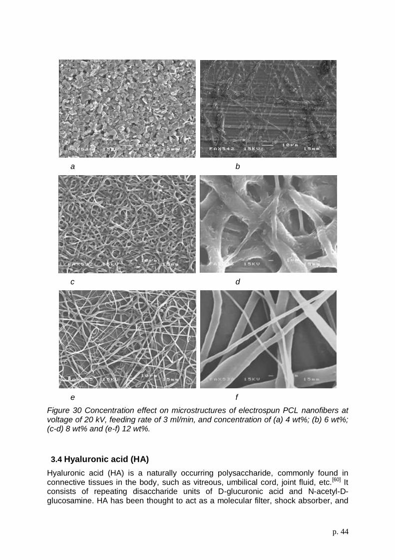
p. 44

a b

c d

e f

Figure 30 Concentration effect on microstructures of electrospun PCL nanofibers at voltage of 20 kV, feeding rate of 3 ml/min, and concentration of (a) 4 wt%; (b) 6 wt%; (c-d) 8 wt% and (e-f) 12 wt%.

3.4 Hyaluronic acid (HA)

Hyaluronic acid (HA) is a naturally occurring polysaccharide, commonly found in connective tissues in the body, such as vitreous, umbilical cord, joint fluid, etc.[60] It consists of repeating disaccharide units of D-glucuronic acid and N-acetyl-D-glucosamine. HA has been thought to act as a molecular filter, shock absorber, and

p. 45

support structure for collagen fibrils[61].Because of its unique rheological properties and complete biocompatibility, HA has been used quite extensively in many biomedical applications, including ophthalmology, drug delivery, dermatology, surgery, and medical implants[62,63].

Fabrication of HA scaffolds

Given amounts of HA powder were dissolved in DMF under gentle stirring for 10 min, and then a specific amount of distilled water was added into the HA solution according to a 50/50 volume ratio of DMF to water. The solution was continuosly stirred for 20 min until it became transparent. A spinning solution of 1.5 w/v% HA in DMF/water system was prepared[64]. In order to process high viscosity solutions such as the ones of HA it was necessary modify the electrospinning apparatus. We have implemented an air blowing addition to the conventional electro-spinning system to expand the capability of the process and to overcome the shortcomings due to the quite high viscosity of HA solutions. This technique is termed “electro-blowing”[65]. For the electro-blowing process, an air blowing system was attached to the electro-spinning apparatus so that the modified apparatus had two simultaneously applied forces (an electrical force and an air-blowing shear force) to fabricate the nanofibers from a polymer fluid. The air blow system consisted of two components, a heater and a blower. The air generated by the blower was heated by passing it through heating elements. The electrospinning solutions, spinneret, and the environmental temperatures were controlled at 40+3°C. The electrospinning solutions were placed into a 5 ml syringe with a capillary tip having an inner diameter of 0.7 mm. A syringe pump was used to feed the polymer solution and the feeding rate was fixed at 60 µl∙min-1. A high-voltage power supply was employed to generate the electric field (0–50 kV). The applied voltage was fixed at 22 kV. The tip-to-collector distance was fixed at 15 cm.

Figure 31 SEM images of HA (1.5 w/v%) fibers at different magnification.

p. 46

Chapter 3 Electrospinning of benzyl ester of hyaluronic acid (HYAFF-11)

1 Introduction

Biodegradable polymers are used for medical applications such as surgical sutures, drug delivery devices, tissue supports, and implants for interior bone fixation[66,67]. Based on the availability of such polymers, tissue engineering became a new approach to reconstruction and/or regeneration of lost or damaged tissue. A variety of porous materials have been used to produce three-dimensional cell composites by allowing individual cells to attach on the scaffold surface, promoting cell growth, and maintaining the differentiated cell phenotypes[68]. For a tissue to be successfully regenerated, sufficient cell propagation, and appropriate differentiation must be achieved in the three-dimensional cellular composite. Nonwoven fabrics are widely used as scaffolds for tissue engineering application[69–71]. However, nonwoven fibrous matrices currently used in tissue engineering have a relatively large porosity, and pore size, in the range of several hundred micrometers, and have not been structurally optimized for specific applications[68,72]. Thus, there is need for a reliable method that can be easily used to modify the microstructure of nonwoven fibrous matrix to be used as a scaffold for tissue engineering applications. A novel biodegradable polymer scaffold based on the electrospun nanofibrous structure is introduced in this study. The non-woven material is composed of benzyl ester of hyaluronic acid (HYAFF-11). Because of its important biological roles, hyaluronic acid has been widely exploited in medical practice for use in treating many different conditions. Several hyaluronic acid containing products are currently marketed for pharmaceutical or veterinary use, including a product for intra ocular injection during eye surgery, synovitis agents for veterinary use and coated gauzes for wound dressings. Through the esterification of carboxyl groups of hyaluronic acid with various therapeutically inactive and active alcohols, it has been possible to synthesize biopolymers with medically desirable properties that are significantly different from those of hyaluronic acid itself. In particular, the esterification prevents fast enzymatic degradation of hyaluronic acid in vivo and allows prolonged scaffold integrity in concert with new tissue formation. The benzyl ester of hyaluronic acid (HYAFF-11) is commercially available as skin repair products for wound and burn patients. To explore the application of electrospinning to this material, morphologies of resultant scaffolds were examined by scanning electron microscope (SEM). Fibrosarcoma cells HT1080 and epithelial CACO-2 cells were seeded on the scaffolds to determine cell proliferation, morphology, and cell–matrix interaction after seeding.

2 Fabrication of HYAFF-11 scaffolds

Polymer solutions were prepared by dissolving the HYAFF-11 (obtained from prof. Vittorio Crescenzi) into 1,1,3,3,3-hexaflouro-2-propanol (HFIP), at the concentrations of 1.01%, 1.15%, 1.22% and 1.34%wt, under gentle stirring for 12 hours. All solutions were prepared at room temperature. Rheological properties of HYAFF-11 solutions are showed in Figure 32. Viscosity vs concentration in the range investigated is presented in Figure 33. For each concentration, 10 g of the polymer solution was

p. 47

loaded into a 10-ml plastic syringe, which was controlled by a syringe pump at a feeding rate of 3.0 ml/h. A glass capillary tube was used to connect the syringe to a needle, which was set up vertically. Needles with an inner diameter of 0.7 mm and cut to a length of 1 cm were used. The distance between the syringe needle tip and the collector was adjusted to 20 cm. A voltage of 15 kV between needle tip and collector was applied by a voltage regulated DC power supply.

Shear Rate [1/s]

0 1 2 3 4 5 6 7 8

vis

cosity [P

a*s

]

0,1

1

10

Shear Rate [1/s]

0 1 2 3 4 5 6 7

vis

cosity [P

a*s

]

0,1

1

10

a b

Shear Rate [1/s]

0 2 4 6 8 10 12

vis

cosity [P

a*s

]

0,1

1

10

Shear Rate [1/s]

0 2 4 6 8 10 12

vis

cosity [P

a*s

]

0,1

1

10

c d

Figure 32 Rheological analysis of HYAFF-11 solutions in HFIP at 25°C; a) 1.01%Wt, b) 1.15%Wt, c) 1.22%Wt d) 1.28%Wt.

p. 48

Concentration [%Wt]

1,0 1,1 1,2 1,3

vis

co

sity [P

a*s

]

0,6

0,8

1,0

1,2

1,4

1,6

Figure 33 Viscosity of HYAFF-11 solutions in HFIP vs concentration at 25°C.

3 Fiber characterization

The morphology of electrospun HYAFF-11 scaffolds was studied by scanning electron microscopy (SEM) with an accelerating voltage of 26 kV. Before the observation, the scaffolds were coated with gold using a sputter coater. The diameter of the fiber was measured from the SEM photographs using image analysis software (Image pro Plus, Media Cybernetics). The experimental variables investigated include solution properties (concentration) and processing parameters (applied electric field and solution flow feeding rate). Their relationships with the membrane microstructure are summarized below.

Effect of applied voltage

It has been observed that the shape of the initiating droplet at the needle tip can be changed by several electrospinning variables, such as applied voltage, viscosity and feeding rate of the polymer solution. We confirm that an increase in the electrospinning voltage can alter the shape of the initial droplet. Consequently, the resulting fiber morphology can be changed from a typical cylindrical shape to a beaded or string-of-pearls structure. In this work, SEM micrographs of nanofibers electrospun at different electrospinning voltage from a constant polymer concentration of 1.34% wt are shown in Figure 34. Fiber diameter tends to decrease with increasing electrospinning voltage, although the influence was not as significant as that of polymer concentration. Figure 35 shows fiber diameter as a function of electrospinning voltage.

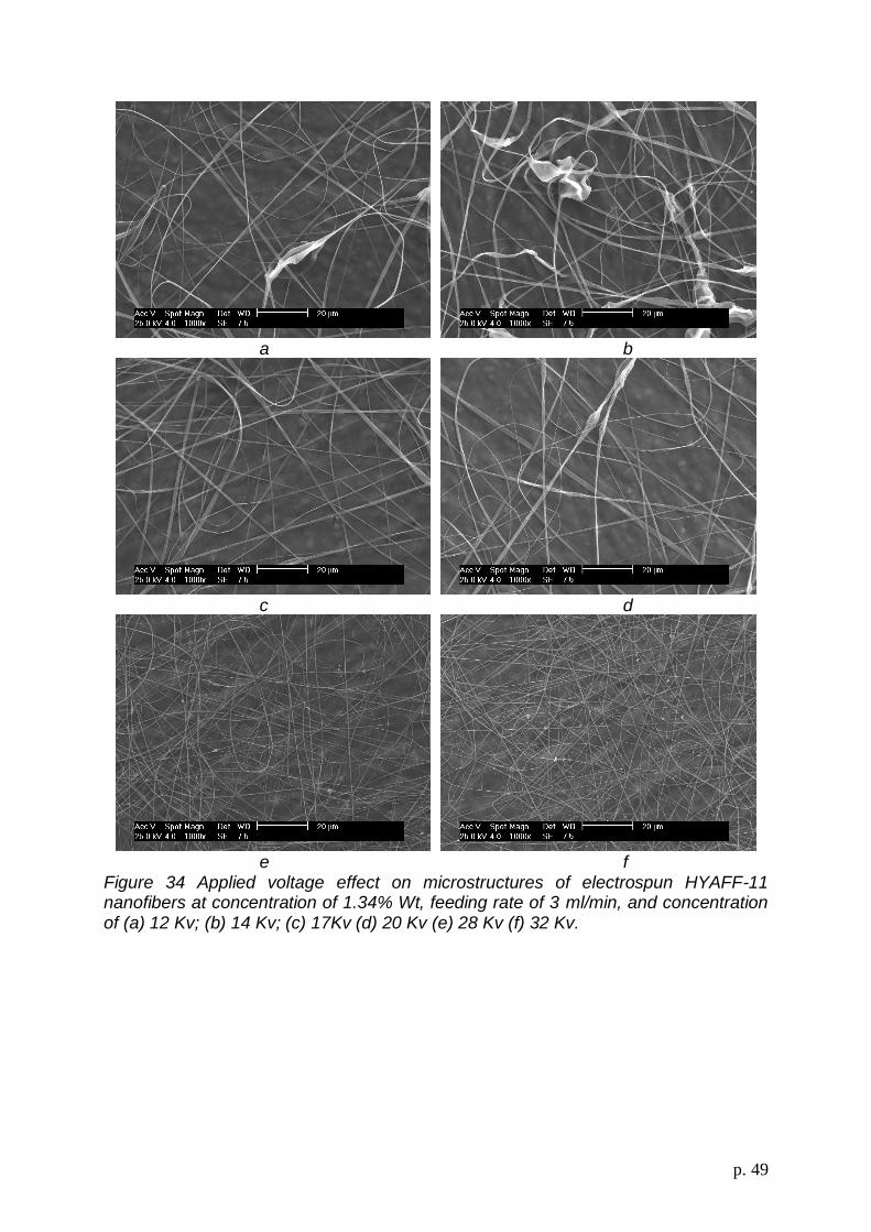
p. 49

a b

c d

e f

Figure 34 Applied voltage effect on microstructures of electrospun HYAFF-11 nanofibers at concentration of 1.34% Wt, feeding rate of 3 ml/min, and concentration of (a) 12 Kv; (b) 14 Kv; (c) 17Kv (d) 20 Kv (e) 28 Kv (f) 32 Kv.

p. 50

Applied Voltage [Kv]

10 15 20 25 30 35

Diameter

[m]

0,3

0,4

0,5

0,6

0,7

0,8

0,9

1,0

Figure 35 Diameter of HYAFF-11 fibers vs applied voltage. Effect of concentration

Drastic morphological changes were found when the concentration of the polymer solution was changed. In other words, the concentration or the corresponding viscosity was one of the most effective variables to control fiber morphology. Figure 33 shows the range of concentrations used in this study for HYAFF-11 in 1,1,3,3,3-hexaflouro-2-propanol and the corresponding viscosities. SEM images of the membranes spun from the HYAFF-11 solutions of different concentration are shown in Figure36 (under a voltage of 28 kV). We were unable to collect a continuous fiber at a concentration below 6 wt%. In Figure36, the SEM images demonstrate the two extreme cases of membrane morphology as a function of solution concentration. The membrane morphology is seen to change gradually from the full beaded structure (Figure36a electrospun at the lowest solution viscosity) to the uniform fiber-structure (Figure36d, at the highest solution viscosity).

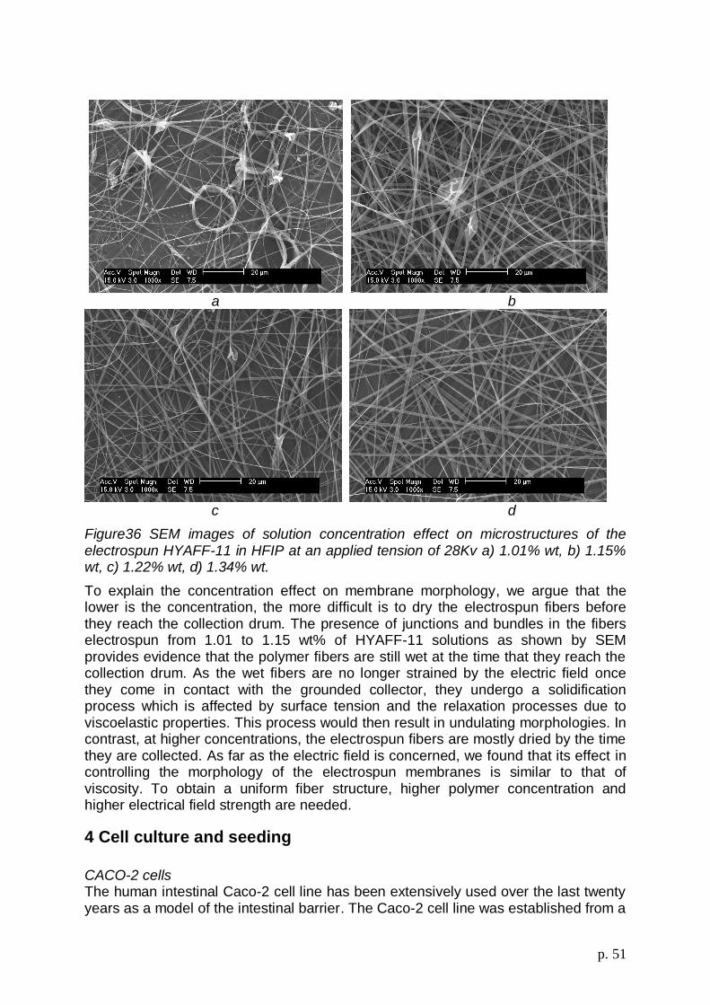
p. 51

a b

c d

Figure36 SEM images of solution concentration effect on microstructures of the electrospun HYAFF-11 in HFIP at an applied tension of 28Kv a) 1.01% wt, b) 1.15% wt, c) 1.22% wt, d) 1.34% wt.

To explain the concentration effect on membrane morphology, we argue that the lower is the concentration, the more difficult is to dry the electrospun fibers before they reach the collection drum. The presence of junctions and bundles in the fibers electrospun from 1.01 to 1.15 wt% of HYAFF-11 solutions as shown by SEM provides evidence that the polymer fibers are still wet at the time that they reach the collection drum. As the wet fibers are no longer strained by the electric field once they come in contact with the grounded collector, they undergo a solidification process which is affected by surface tension and the relaxation processes due to viscoelastic properties. This process would then result in undulating morphologies. In contrast, at higher concentrations, the electrospun fibers are mostly dried by the time they are collected. As far as the electric field is concerned, we found that its effect in controlling the morphology of the electrospun membranes is similar to that of viscosity. To obtain a uniform fiber structure, higher polymer concentration and higher electrical field strength are needed.

4 Cell culture and seeding

CACO-2 cells The human intestinal Caco-2 cell line has been extensively used over the last twenty years as a model of the intestinal barrier. The Caco-2 cell line was established from a

p. 52

moderately well differentiated colon adenocarcinoma obtained from a 72-year-old patient (Fogh et al. 1977). Caco-2 cells differentiate spontaneously in culture and exhibit structural and functional differentiation patterns characteristic of mature enterocytes (Pinto et al. 1983). Caco-2 cells reach confluency within 3-6 days and reach the stationary growth phase after 10 days in culture (Braun et al. 2000). The differentiation is completed within 20 days (Pinto et al. 1983). The differentiated cells exhibit high levels of alkaline phosphatase, sucrase isomaltase and aminopeptidase activity characteristic of enterocyte brush border microvilli. The structural and functional differentiation of the microvilli is associated with the polarization of the monolayer after confluency. Fully differentiated Caco-2 cells form an epithelial membrane with a barrier function similar to the human colon (Artursson et al., 1993) but express carrier proteins similar to the small intestine (Baker and Baker 1992, Hidalgo et al. 1989, Wilson et al. 1990). Caco-2 cell monolayers have been used for studying mechanisms of passive paracellular (Artursson et al., 1993, Artursson et al. 1996, and many others) and passive transcellular permeability (Artursson 1990 and others), carrier mediated absorptive transport of amino acids, amino acid analogues, oligopeptides , ß-lactam antibiotics and ACE-inhibitors, and peptidomimetic thrombin inhibitors. Carrier mediated efflux (combined with metabolism inside the enterocytes) of several drugs has been intensively studied over the last years, as well as cocktail dosing of several different drugs. The cells were cultured with Dulbecco´s Modified Eagle´s Medium (DMEM) supplemented with 10% heat inactivated foetal bovine serum and 1% non-essential amino acids, 1% L-glutamine and 100 IU/ml penicillin + 100 μg/ml streptomycin. All cell culture media were obtained from Gibco Invitrogen Corp. After reaching about 70% confluence, the cells were detached by 0.05% trypsin and viable cells were counted by the trypan blue assay. The cells were then seeded onto HYAFF-11 scaffolds, placed on a cover glass and then in a 6-well plate at the density of 2.8x104 cells/cm2. Live cell morphology was studied by using an inverted phase contrast light microscope The phase contrast micrographs shown in Figure 37 a-c were taken on cells attached to the scaffolds after one hour, two days, and six days of cell seeding at random locations in each scaffolds In Figure 37d a confocal image of the cell-produced extracellular matrix (ECM) is shown, the green color being due to ECM auto-fluorescence.

p. 53

a b

c d

Figure 37 Images of CACO-2 cell seeded on electrospun HYAFF-11 scaffolds: a) after 1 hour of culture; b) after 2 days of culture and c-d) after 6 days of culture. Fibrosarcoma HT-1080 This cell line was obtained starting from a biopsy in July, 1972 from a fibrosarcoma arising adjacent to the acetabulum of a 35-year-old Caucasian man. At death he had clinical evidence of widespread metastatic tumor. The histopathologic diagnosis of the biopsy specimen was poorly differentiated fibrosarcoma. Usually fibrosarcoma cell line is used as a model system because these cells, like tumor stromal fibroblasts, express several MMPs. In this work, the HT1080 cell suspension was seeded in 75 cm2 Falcon flasks and 100 mm dishes, and the excess medium was aspirated. The flasks were left at an angle of ca 60° for 5-10 minutes before adding 7-8 ml of culture medium. This procedure helped the cells to attach to the surface of the flask or dish. The cell suspension was filtered through a loose mesh gauze to exclude the larger clumps. The cells were routinely cultured in tissue culture polystyrene flasks at 37°C under 5% CO2 atmosphere and the culture medium was DMEM medium containing 10% FBS and antibiotics. Once the cells reached 80% confluency, they were trypsinized and seeded onto the surface of nanofiber matrixes attached to the bottom of multi-well plates at a seeding density of 50,000 cells/well. The phase contrast micrographs in Figure 38 were taken at random locations in each scaffold after five hours, seven hours, thirty one hours and forty six hours from cell seeding.

p. 54

a b

c d

Figure 38 Images of fibrosarcoma cell HT1080 seeded on electrospun HYAFF-11 scaffolds: a) after 5 hours of culture; b) after 7hours of culture c) after 31 hours and d) after 47 hours of culture.

5 Cell proliferation studies

The CACO-2 cell proliferation on electrospun HYAFF-11 scaffolds was compared with the morphology and proliferation of the same cell on scaffolds obtained from the electrospinning of PLA solutions and PCL solutions. To perform this experiment we have used the time lapse technique. Time lapse experiments The time-lapse microscopy technique allows continuously observing and recording phenomena that can last up to several days. By means of motorized sample positioning, multiple fields of view can be imaged in an iterative fashion, in order to ensure reproducibility and statistical significance of the collected data. Time-lapse live cell imaging requires the right environmental conditions (i.e temperature, humidity and CO2 concentration) under the microscope stage. This was achieved in this work by using a microscope cage incubator (Okolab, Italy), which enclose the whole microscope and allows to maintain the cells, plated in a multi-well plate, in a 5% CO2 atmosphere at 37◦C. To avoid humidity-induced damage to the the mechanical and electrical parts of the microscope, the samples were placed inside a small chamber on the microscope stage where a suitable microenvironment for live cell imaging was created by feeding a pre-heated humidified air stream with the desired CO2 concentration. Time-lapse video microscopy was performed by using a

p. 55

Zeiss Axiovert 200 inverted microscope with a 20×long working distance objective. Z-stacks of images along the sample depth were acquired at several x-y positions in an iterative fashion by using a time-lapse software (Okolab), which allows the user to select the fields of view to be imaged at a given time interval (10 min in this case). The time-lapse software controls the operation of an x-y motorized stage (Ludl, USA), a motorized focus stage (Ludl, USA) and a video camera (Hamamatsu, Japan). The setup of the time-lapse microscopy workstation is shown schematically in Figure 39.

Figure 39 Time-lapse microscopy workstation To measure cell proliferation the images were processed by Image Pro plus as shown in Figure 40a. The contour of cells is drawn on the image in a semi-automated way in order to measure the cellular area (Figure 40b).

a b

Figure 40 a) software window b) image of cell clusters with outlined contour.

p. 56

Images taken during time-lapse experiments on CACO-2 cells are shown in c d Figure 41 (a-d) for electrospun HYAFF-11 scaffolds, in Figure 42 (a-d) for electrospun PLA scaffolds and in c d Figure 43 (a-d) for electrospun PCL scaffolds.

a b

c d

Figure 41 Images of CACO-2 cell seeded on electrospun HYAFF-11 scaffolds: a) after 5 minutes of culture; b) after 10 hours of culture c) after 21 hours culture and d) after 43 hours of culture.

p. 57

a b

c d

Figure 42 Images of CACO-2 cell seeded on electrospun PLA scaffolds: a) after 5 minutes of culture; b) after 10 hours of culture c) after 21 hours culture and d) after 43 hours of culture.

p. 58

a b

c d

Figure 43 Images of CACO-2 cell seeded on electrospun PCL scaffolds: a) after 5 minutes of culture; b) after 10 hours of culture c) after 21 hours culture and d) after 43 hours of culture. Image analysis of the time-lapse experiments shows that the cells seeded on electrospun HYAFF-11 scaffolds grow faster then cells seeded on the other electrospun scaffolds. This is shown in Figure 44, where the average cell area, normalized with respect to the initial value, is plotted as a function of time.

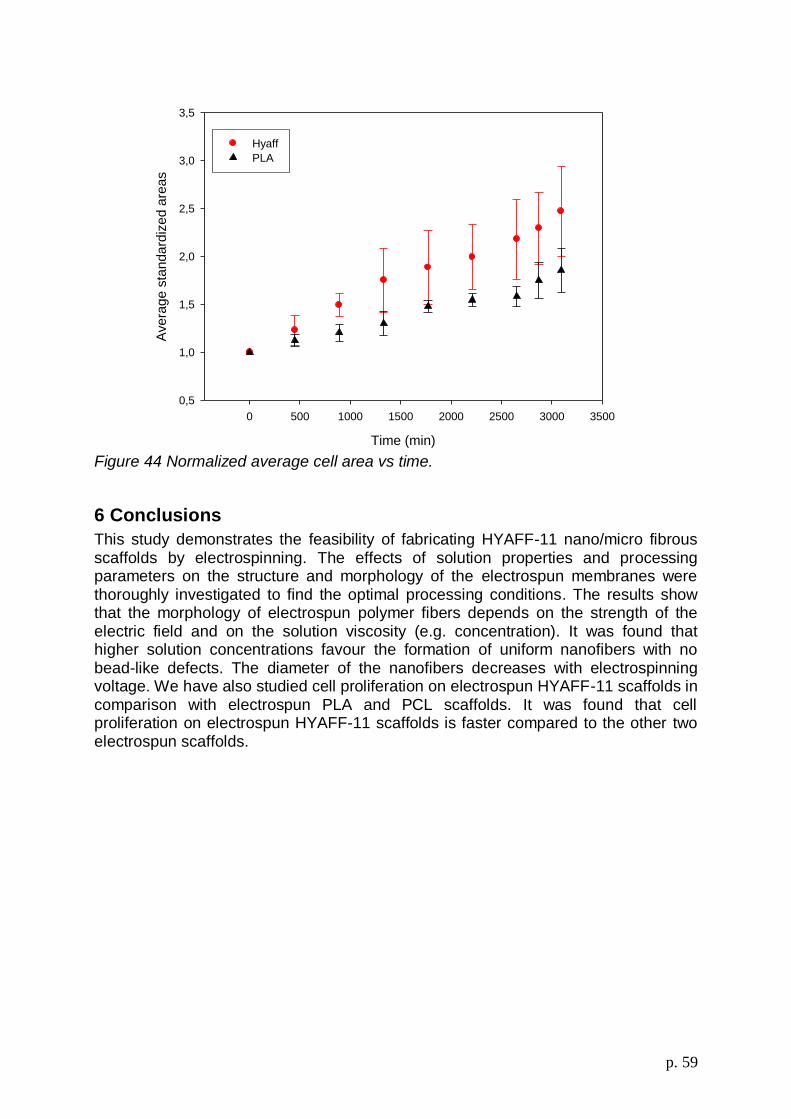
p. 59

Time (min)

0 500 1000 1500 2000 2500 3000 3500

Ave

rag

e s

tan

da

rdiz

ed

are

as

0,5

1,0

1,5

2,0

2,5

3,0

3,5

Hyaff

PLA

Figure 44 Normalized average cell area vs time.

6 Conclusions

This study demonstrates the feasibility of fabricating HYAFF-11 nano/micro fibrous scaffolds by electrospinning. The effects of solution properties and processing parameters on the structure and morphology of the electrospun membranes were thoroughly investigated to find the optimal processing conditions. The results show that the morphology of electrospun polymer fibers depends on the strength of the electric field and on the solution viscosity (e.g. concentration). It was found that higher solution concentrations favour the formation of uniform nanofibers with no bead-like defects. The diameter of the nanofibers decreases with electrospinning voltage. We have also studied cell proliferation on electrospun HYAFF-11 scaffolds in comparison with electrospun PLA and PCL scaffolds. It was found that cell proliferation on electrospun HYAFF-11 scaffolds is faster compared to the other two electrospun scaffolds.

p. 60

Chapter 4 DISPERSION OF NANOPARTICLES BY ELECTROSPINNING PROCESS

1 Introduction

Nanoparticle-based materials have been attracting a growing interest in the fields of physics (quantum optics), chemistry (catalysts), and nanotechnology. The main reason of such interest is that chemical and physical properties of nanocomposites are quite different from those of bulk materials. However, the main difficulty in working with nanoparticles is their undesirable tendency to form larger particles by agglomeration. To prevent formation of aggregates, surfactants[78,79], ligand exchange materials[80,81], and polymeric carriers[82] have been extensively used. The approach that has been adopted in this work is to include nanoparticles directly into electrospun fibers from polymer solutions, thus circumventing the problem of particle aggregation. In the present work, the electrospinning technique has been used to disperse sepiolites (SEP) into large surface area fibers.

2 Sepiolite

Sepiolite, formerly known as Meerschaum (sea froth), is a non-swelling, lightweight, porous clay with a large specific surface area. Unlike other clays, the individual particles of sepiolite have a needle-like morphology. The high surface area and porosity, as well as the unusual particle shape of this clay account for its outstanding sorption capacity and colloidal properties that make it a valuable material for a wide range of applications. Sepiolite is a very uncommon clay because of both its peculiar features and scarce occurrence. There are very few commercial deposits in the world. Most of the world production of this clay comes from deposits of sedimentary origin located near Madrid, Spain. Chemically, sepiolite is a hydrated magnesium silicate with the ideal formula Si12Mg8O30(OH)4(OH2)4.8H2O. Sepiolite, unlike other clays, is not a layered phyllosilicate. Its structure can be described as a quincunx (an arrangement of five objects, so placed that four occupy the corners and the fifth the centre of a square or rectangle, see Figure 45) of talc-type sheets separated by parallel channels. This chain-like structure produces needle-like particles instead of plate-like particles like other clays.

Figure 45 Structure of sepiolite

p. 61

Sepiolite has the highest surface area (BET, N2) of all the clay minerals, about 300 m2/g, with a high density of silanol groups (-SiOH) which explains the marked hydrophilicity of this clay. The silicate lattice has not a significant negative charge and therefore the cation exchange capacity of this clay is very low. The tiny elongated particles of sepiolite have an average length of 1μm to 2 μm, a width of 0.01 μm, and contain open channels with dimensions of 3.6 Å x 10.6 Å running along the axis of the particle (Figure 46). These particles are arranged in such a way to form loosely packed and porous aggregates with an extensive capillary network which explains the high porosity of sepiolite and its light weight due the large void space. The high surface area and porosity of sepiolite account for the remarkable adsorptive and absorptive properties of this clay. It adsorbs vapours and odours and can absorb approximately its own weight of water and other liquids. Sepiolite is a non-swelling clay and its granules do not disintegrate even when saturated with liquids. Colloidal grades of sepiolite must be dispersed into water or other liquid systems using high-shear mixers. Once dispersed in the liquid, it forms a structure of randomly intermeshed elongated particles, which is maintained by physical interference and hydrogen bonding, and entraps the liquid, thus increasing the viscosity of the suspension. This structure is stable even in systems with high salt concentrations, conditions that produce the flocculation of other clay suspensions, such as bentonite.

Figure 46 SEM image of sepiolite particles

The random network of sepiolite particles holds coarser particles in the liquid preventing their settling by gravity, acting as a suspending agent. Sepiolite provides to its suspensions a pseudoplastic and thixotropic behaviour which make it a valuable material in multiple applications to improve processability, application or handling of the final product.

3 Preliminary work

PEO of average weight molecular weight of 9 x 105 (g/mol) and distilled water were used. The solutions were prepared at room temperature, and gently stirred to speed up dissolution at concentrations of 7% w/w. SEP was added so as to have a ratio SEP/PEO equal to 0.05. In this condition, however, water promotes the formation of clusters as shown in Figure 47.

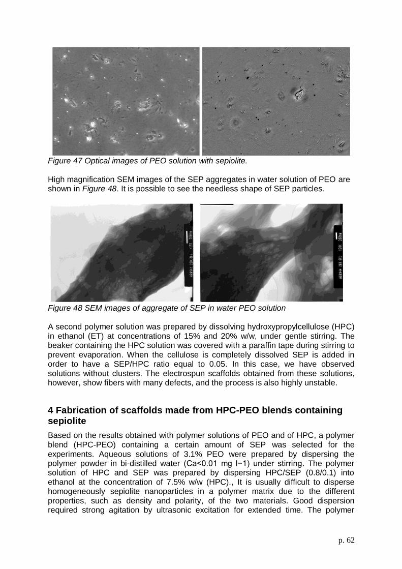
p. 62

Figure 47 Optical images of PEO solution with sepiolite.

High magnification SEM images of the SEP aggregates in water solution of PEO are shown in Figure 48. It is possible to see the needless shape of SEP particles.

Figure 48 SEM images of aggregate of SEP in water PEO solution A second polymer solution was prepared by dissolving hydroxypropylcellulose (HPC) in ethanol (ET) at concentrations of 15% and 20% w/w, under gentle stirring. The beaker containing the HPC solution was covered with a paraffin tape during stirring to prevent evaporation. When the cellulose is completely dissolved SEP is added in order to have a SEP/HPC ratio equal to 0.05. In this case, we have observed solutions without clusters. The electrospun scaffolds obtained from these solutions, however, show fibers with many defects, and the process is also highly unstable.

4 Fabrication of scaffolds made from HPC-PEO blends containing sepiolite

Based on the results obtained with polymer solutions of PEO and of HPC, a polymer blend (HPC-PEO) containing a certain amount of SEP was selected for the experiments. Aqueous solutions of 3.1% PEO were prepared by dispersing the polymer powder in bi-distilled water (Ca<0.01 mg l−1) under stirring. The polymer solution of HPC and SEP was prepared by dispersing HPC/SEP (0.8/0.1) into ethanol at the concentration of 7.5% w/w (HPC)., It is usually difficult to disperse homogeneously sepiolite nanoparticles in a polymer matrix due to the different properties, such as density and polarity, of the two materials. Good dispersion required strong agitation by ultrasonic excitation for extended time. The polymer

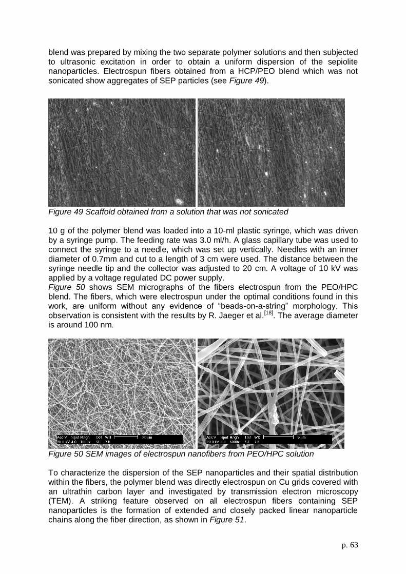
p. 63

blend was prepared by mixing the two separate polymer solutions and then subjected to ultrasonic excitation in order to obtain a uniform dispersion of the sepiolite nanoparticles. Electrospun fibers obtained from a HCP/PEO blend which was not sonicated show aggregates of SEP particles (see Figure 49).

Figure 49 Scaffold obtained from a solution that was not sonicated 10 g of the polymer blend was loaded into a 10-ml plastic syringe, which was driven by a syringe pump. The feeding rate was 3.0 ml/h. A glass capillary tube was used to connect the syringe to a needle, which was set up vertically. Needles with an inner diameter of 0.7mm and cut to a length of 3 cm were used. The distance between the syringe needle tip and the collector was adjusted to 20 cm. A voltage of 10 kV was applied by a voltage regulated DC power supply. Figure 50 shows SEM micrographs of the fibers electrospun from the PEO/HPC blend. The fibers, which were electrospun under the optimal conditions found in this work, are uniform without any evidence of “beads-on-a-string” morphology. This observation is consistent with the results by R. Jaeger et al.[18]. The average diameter is around 100 nm.

Figure 50 SEM images of electrospun nanofibers from PEO/HPC solution To characterize the dispersion of the SEP nanoparticles and their spatial distribution within the fibers, the polymer blend was directly electrospun on Cu grids covered with an ultrathin carbon layer and investigated by transmission electron microscopy (TEM). A striking feature observed on all electrospun fibers containing SEP nanoparticles is the formation of extended and closely packed linear nanoparticle chains along the fiber direction, as shown in Figure 51.

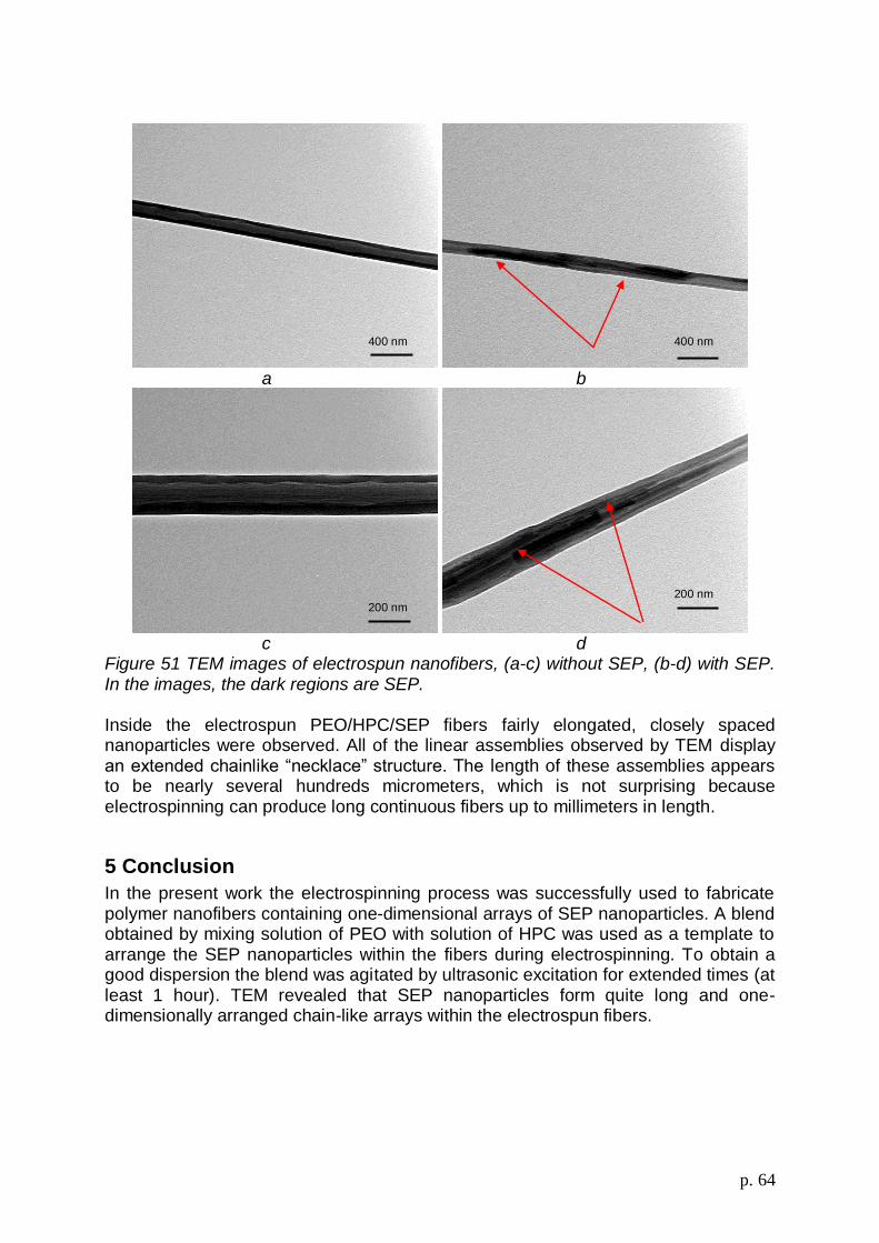
p. 64

a b

c d

Figure 51 TEM images of electrospun nanofibers, (a-c) without SEP, (b-d) with SEP. In the images, the dark regions are SEP. Inside the electrospun PEO/HPC/SEP fibers fairly elongated, closely spaced nanoparticles were observed. All of the linear assemblies observed by TEM display an extended chainlike “necklace” structure. The length of these assemblies appears to be nearly several hundreds micrometers, which is not surprising because electrospinning can produce long continuous fibers up to millimeters in length.

5 Conclusion

In the present work the electrospinning process was successfully used to fabricate polymer nanofibers containing one-dimensional arrays of SEP nanoparticles. A blend obtained by mixing solution of PEO with solution of HPC was used as a template to arrange the SEP nanoparticles within the fibers during electrospinning. To obtain a good dispersion the blend was agitated by ultrasonic excitation for extended times (at least 1 hour). TEM revealed that SEP nanoparticles form quite long and one-dimensionally arranged chain-like arrays within the electrospun fibers.

200 nm 200 nm

400 nm 200 nm

200 nm

200 nm

400 nm 200 nm

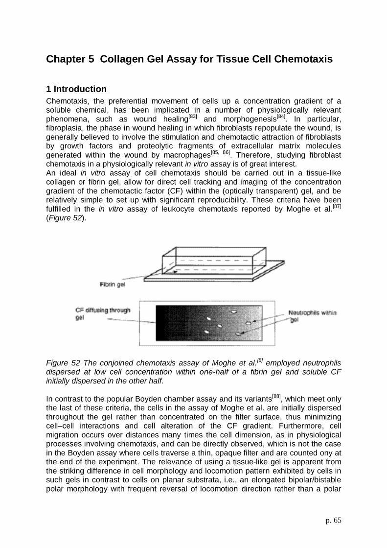
p. 65

Chapter 5 Collagen Gel Assay for Tissue Cell Chemotaxis

1 Introduction

Chemotaxis, the preferential movement of cells up a concentration gradient of a soluble chemical, has been implicated in a number of physiologically relevant phenomena, such as wound healing[83] and morphogenesis[84]. In particular, fibroplasia, the phase in wound healing in which fibroblasts repopulate the wound, is generally believed to involve the stimulation and chemotactic attraction of fibroblasts by growth factors and proteolytic fragments of extracellular matrix molecules generated within the wound by macrophages[85, 86]. Therefore, studying fibroblast chemotaxis in a physiologically relevant in vitro assay is of great interest. An ideal in vitro assay of cell chemotaxis should be carried out in a tissue-like collagen or fibrin gel, allow for direct cell tracking and imaging of the concentration gradient of the chemotactic factor (CF) within the (optically transparent) gel, and be relatively simple to set up with significant reproducibility. These criteria have been fulfilled in the in vitro assay of leukocyte chemotaxis reported by Moghe et al.[87] (Figure 52).

Figure 52 The conjoined chemotaxis assay of Moghe et al.[5] employed neutrophils dispersed at low cell concentration within one-half of a fibrin gel and soluble CF initially dispersed in the other half. In contrast to the popular Boyden chamber assay and its variants[88], which meet only the last of these criteria, the cells in the assay of Moghe et al. are initially dispersed throughout the gel rather than concentrated on the filter surface, thus minimizing cell–cell interactions and cell alteration of the CF gradient. Furthermore, cell migration occurs over distances many times the cell dimension, as in physiological processes involving chemotaxis, and can be directly observed, which is not the case in the Boyden assay where cells traverse a thin, opaque filter and are counted ony at the end of the experiment. The relevance of using a tissue-like gel is apparent from the striking difference in cell morphology and locomotion pattern exhibited by cells in such gels in contrast to cells on planar substrata, i.e., an elongated bipolar/bistable polar morphology with frequent reversal of locomotion direction rather than a polar

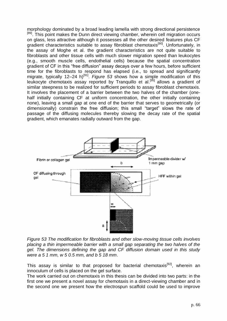
p. 66

morphology dominated by a broad leading lamella with strong directional persistence [89]. This point makes the Dunn direct viewing chamber, wherein cell migration occurs on glass, less attractive although it possesses all the other desired features plus CF gradient characteristics suitable to assay fibroblast chemotaxis[90]. Unfortunately, in the assay of Moghe et al. the gradient characteristics are not quite suitable to fibroblasts and other tissue cells with much slower migration speed than leukocytes (e.g., smooth muscle cells, endothelial cells) because the spatial concentration gradient of CF in this “free diffusion” assay decays over a few hours, before sufficient time for the fibroblasts to respond has elapsed (i.e., to spread and significantly migrate, typically 12–24 h)[91]. Figure 53 shows how a simple modification of this leukocyte chemotaxis assay reported by Tranquillo et al.[95] allows a gradient of similar steepness to be realized for sufficient periods to assay fibroblast chemotaxis. It involves the placement of a barrier between the two halves of the chamber (one-half initially containing CF at uniform concentration, the other initially containing none), leaving a small gap at one end of the barrier that serves to geometrically (or dimensionally) constrain the free diffusion; this small “target” slows the rate of passage of the diffusing molecules thereby slowing the decay rate of the spatial gradient, which emanates radially outward from the gap.

Figure 53 The modification for fibroblasts and other slow-moving tissue cells involves placing a thin impermeable barrier with a small gap separating the two halves of the gel. The dimensions defining the gap and CF diffusion domain used in this study were a 5 1 mm, w 5 0.5 mm, and b 5 18 mm. This assay is similar to that proposed for bacterial chemotaxis[92], wherein an innoculum of cells is placed on the gel surface. The work carried out on chemotaxis in this thesis can be divided into two parts: in the first one we present a novel assay for chemotaxis in a direct-viewing chamber and in the second one we present how the electrospun scaffold could be used to improve

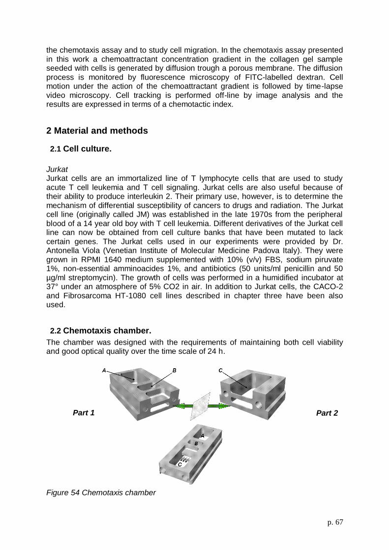
p. 67

the chemotaxis assay and to study cell migration. In the chemotaxis assay presented in this work a chemoattractant concentration gradient in the collagen gel sample seeded with cells is generated by diffusion trough a porous membrane. The diffusion process is monitored by fluorescence microscopy of FITC-labelled dextran. Cell motion under the action of the chemoattractant gradient is followed by time-lapse video microscopy. Cell tracking is performed off-line by image analysis and the results are expressed in terms of a chemotactic index.

2 Material and methods

2.1 Cell culture.

Jurkat Jurkat cells are an immortalized line of T lymphocyte cells that are used to study acute T cell leukemia and T cell signaling. Jurkat cells are also useful because of their ability to produce interleukin 2. Their primary use, however, is to determine the mechanism of differential susceptibility of cancers to drugs and radiation. The Jurkat cell line (originally called JM) was established in the late 1970s from the peripheral blood of a 14 year old boy with T cell leukemia. Different derivatives of the Jurkat cell line can now be obtained from cell culture banks that have been mutated to lack certain genes. The Jurkat cells used in our experiments were provided by Dr. Antonella Viola (Venetian Institute of Molecular Medicine Padova Italy). They were grown in RPMI 1640 medium supplemented with 10% (v/v) FBS, sodium piruvate 1%, non-essential amminoacides 1%, and antibiotics (50 units/ml penicillin and 50 µg/ml streptomycin). The growth of cells was performed in a humidified incubator at 37° under an atmosphere of 5% CO2 in air. In addition to Jurkat cells, the CACO-2 and Fibrosarcoma HT-1080 cell lines described in chapter three have been also used.

2.2 Chemotaxis chamber.

The chamber was designed with the requirements of maintaining both cell viability and good optical quality over the time scale of 24 h.

Figure 54 Chemotaxis chamber

Part 1 Part 2

p. 68

The chambers, shown in Figure 54, consist of two steel blocks glued on top of a microscope slide by using a silicone adhesive. The blocks are separated by a porous membrane and assembled together by two mounting screws. Part 1 in Figure 54 has two compartments; one (A) used as the control well and the other (B) as the reservoir of the chemoattractant solutions. At one side of the B compartment a recess ending in a rectangular open frame is used to minimize possible lens effects due the free interface of the gel in contact with the steel surface next to the membrane. In part 2 there is only one compartment which is used for the cell seeded collagen gel. The membrane separating the chemoattractant and the gel well is sandwiched between the two rectangular open frames in part 1 and 2.

2.3 Preparation of chemotaxis assays.

Collagen gels are prepared with the following composition (volume basis): DMEM (2%), 0.1 M NaOH (13.2%), 10X minimum essential medium (10%), FBS (6.7%), P/S (0.1%), L-glutamine (1%), and Vitrogen 100 collagen solution (67%) (Celtrix Laboratories). Cells suspended in DMEM with 10% FBS are added to the mixture in such a way that the initial cell concentration is between 103 and 104 cells/ml. A low cell concentration is desired in order to minimize cell restructuring of the fibril orientation. The collagen solution is placed in the A and C compartments of the chamber, which has been preliminarly sterilized in an autoclave. Collagen gelification is allowed to occur in a humidified incubator at 37°C.

2.4 Collagen gel birefringence

Since collagen fibrils can become aligned near a surface as the gel forms[96] or within the gel as it compacts due to traction exerted by entrapped cells[97], the possible contributions of contact guidance to directional cell migration and orientation needs to be considered. Restricting measurements to regions of the gel at least 1 mm from surfaces mitigated any surface-induced alignment effects and using low cell concentrations prevented any significant gel compaction during the 24-h observation period. The absence of any contact guidance effects was supported by the random cell orientation measured in the control sample without chemoattractant, shown in Figure 70a. This was also supported by polarized light microscopy examination of the gel region analyzed for cell alignment after the observation period, which did not show a significant or systematic birefringence pattern in the bulk of the gel (data not shown). Birefringence, a measure of the strength of fibril alignment, was measured by placing a guidance chamber between crossed polarizers on a microscope equipped with a CCD camera. Light intensity vs orientation was measured as the guidance chamber was rotated through 5° increments with and without a compensator in the optical path by using the microscopy/image analysis system. However, a cell can induce fibril alignment around itself, a phenomenon which is termed tractional structuring[98], and can influence the alignment of the cell. The possibility exists that fibril alignment due to tractional structuring by a cell responding chemotactically might induce a local contact guidance response that “amplifies” its chemotactic response. The extent to which this occurs will depend on the mechanical and structural properties of the gel, as determined by the gel preparation. For example, “stiffer” networks of fibrils due to increased crosslinking would be less susceptible to tractional structuring by the cells and suppress such amplification.

p. 69

2.5 CF concentration profile measurements.

To study chemoattractant diffusion a fluorescently labeled dextran was used (FITC-dextran). The FITC-dextran selected for the experiments has a molecular weight comparable to that of the chemoattractants investigated, so that a similar diffusion behavior can be assumed. By using the confocal microscope, the mean grey level, which is proportional to fluorescensce intensity, was measured as a function of time and position to characterize the propagation of FITC-dextran front in the collagen gel. To interpret and translate these results in terms of concentrations of FITC-dextran, a calibration is needed. To perform the calibration collagen gels with FITC dextran concentrations in the range 0.2 μ M - 70 μ M were prepared. The solutions were then loaded in a multiwell plate, which was incubated for 40 minutes to allow collagen gelification. Fluorescence images were acquired within each well by using the same. settings of laser power and contrast. The mean gray level, as calculated from the image histogram, was then plotted as a function of FITC-dextran concentration. As shown in Figure 55 a linear trend is found.

y = 13,053x + 8,6818

0

10

20

30

40

50

60

70

80

0 1 2 3 4 5 6

Conc [microM]

Mean

Gra

y L

evel

Figure 55 The calibration curve of mean gray level vs FITC-dextran concentration In order to determine the diffusion coefficient of FITC-dextran a dynamic experiment was performed in the chemotaxis chamber to measure the mean grey level in eight fields of view arranged in pairs at gradually increasing distance from the porous membrane. Each pair is at a certain distance from the membrane (along the x-axis). A schematic of the arrangement of the selected fields of view is shown in Figure 56

p. 70

Figure 56 Schematic of sample scanning areas Measurements of the FITC–dextran gradient were made at 0.5, 12, and 24 h after loading the chemoattractant well. The specific gradient, a scaled measure of CF gradient steepness, was calculated as:

)(

1)(

xcdx

xdc

where c(x) is the concentration of CF at position x. An analytical approximation of the concentration gradient was obtained by assuming the model of free diffusion of Fick. By invoking the symmetry of our assay chamber, we approximated the steady concentration at the membrane as CO/2, where CO is the initial CF concentration in the chemoattractant well. In addition, we assumed that CF could not diffuse across the chamber walls (i.e., C=0 x ∞) and applied the initial condition consistent with no CF being initially present in one-half of the chamber {C=0, t=0}. The resulting expression, i.e.,

Dt

xerf

CC

41

2

0

was fit to experimental data to determine the diffusion coefficient of FITC-dextran, wich turned out ca.2x10-6 cm2/sec, in good agreement with data from the literature.

a b

Figure 57 a) Fluorescence image of FITC-dextran b) Surface plot of image

Porous membrane

p. 71

Figure 58 shows the concentration profile of FITC–dextran as a function of distance outward from the gap. The concentration decreased exponentially with distance at each time (1, 15 and 24 h). The measured profiles of the specific gradient compare favorably to those predicted from the analytical solution. The value of specific gradient was in the range 0.01-0.1 in good agreement of literature.

a b

c d

Figure 58 concentration profile of FITC–Dextran as a function of distance outward from the gap at different time a)1h b)16h c). d) Profile of the specific gradient as a function of distance outward from the gap

3 Preparation of trans-epithelial assays by the electrospinning process

This assay involves a two-compartment system where cells may be induced to migrate from an upper compartment through a electrospun porous membrane into a lower compartment (or viceversa), thus following the gradient of a chemoattractant (see Figure 59). Relative to the size of the investigated cells, the size of the pores in the membrane must be small enough to avoid the passive passage of cells by gravity or convection, but large enough to allow their active migration. Our test improves those currently

p. 72

available because we use a porous membrane obtained from a solution of a biopolymer instead of synthetic polymers.

Figure 59 Experimental setup to study cell invasion in vitro The membrane on the cell culture inserts of the transwell was obtained by direct exposition to the jets of fibers generated from the needle of the electrospinning apparatus as shown in Figure 60a. Figure 60b shows cell culture inserts when the process of electrospinning was completed. The so obtained cell culture inserts are placed in a multiwell plate, thereby forming two compartments: the upper compartment of the insert and the lower compartment of the plate well. The two compartments form the migration chamber, separated by the porous biopolymer membrane as shown in Figure 59. Cells sedimenting onto the membrane from the surrounding medium may be induced to actively migrate through the membrane into the lower compartment by serum or other chemoattractants.

a b

Figure 60 a) Formation of electrospun membrane onto cell culture insert b) Cell culture insert with electrospun membrane In order to perform a transepithelial migration assay ephithelial cells were cultured on the membrane. Cell cultures were prepared and maintained according to the standard cell culture procedures previously described. For migration assays, 3–4 x103 CACO-2 cell cells were plated onto electrospun membranes of transwell cell culture inserts. Depending on the cell orientation desired, cells were plated on either the top of membranes (apical surface up) or the bottom of membranes by inversion of

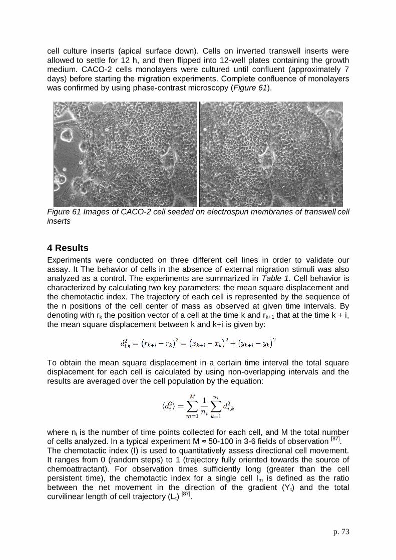
p. 73

cell culture inserts (apical surface down). Cells on inverted transwell inserts were allowed to settle for 12 h, and then flipped into 12-well plates containing the growth medium. CACO-2 cells monolayers were cultured until confluent (approximately 7 days) before starting the migration experiments. Complete confluence of monolayers was confirmed by using phase-contrast microscopy (Figure 61).

Figure 61 Images of CACO-2 cell seeded on electrospun membranes of transwell cell inserts

4 Results

Experiments were conducted on three different cell lines in order to validate our assay. It The behavior of cells in the absence of external migration stimuli was also analyzed as a control. The experiments are summarized in Table 1. Cell behavior is characterized by calculating two key parameters: the mean square displacement and the chemotactic index. The trajectory of each cell is represented by the sequence of the n positions of the cell center of mass as observed at given time intervals. By denoting with rk the position vector of a cell at the time k and rk+1 that at the time k + i, the mean square displacement between k and k+i is given by:

To obtain the mean square displacement in a certain time interval the total square displacement for each cell is calculated by using non-overlapping intervals and the results are averaged over the cell population by the equation:

where ni is the number of time points collected for each cell, and M the total number of cells analyzed. In a typical experiment M ≈ 50-100 in 3-6 fields of observation [87]. The chemotactic index (I) is used to quantitatively assess directional cell movement. It ranges from 0 (random steps) to 1 (trajectory fully oriented towards the source of chemoattractant). For observation times sufficiently long (greater than the cell persistent time), the chemotactic index for a single cell Im is defined as the ratio between the net movement in the direction of the gradient (Yt) and the total curvilinear length of cell trajectory (Lt)

[87].

p. 74

Cell line #. cells

analized

#. field of

view

#. layers Cell seded

Thickness of gel (μm)

Chemoattractant

Jurkat CCR5 GFP

47 2 30 200000 1732 Rantes 50 nM

Jurkat CCR5 GFP

147 2 30 245000 1734 Rantes 50 nM

Jurkat 96 2 50 170000 5277 SDF 1 nM

Lymphocyte 55 3 40 254000 4054 SDF 4.5 nM

Lymphocyte 336 4 40 358000 3229 SDF 4.5 nM

Lymphocyte 162 3 40 315800 4049 SDF 4.5 nM

Fibrobalst 106 4 40 80000 4054 FBS

Fibrobalst 61 3 15 80800 1108 FBS

Fibrobalst 731 23

50

82000

485

Jurkat (control)

111 2 50 220000 978

Table 1 Table of tests Im = Yt / Lt Where Yt = yk–y1

Lk = [(x2–x1)*2 + (y2–y1)*2 + (x3–x2)*2 + (y3–y2)*2 + ... + (xk – xk-1)2 + (yk – yk-1)2]1/2 for t = kΔt The value of I is determined by averaging the Im values weighted on the trajectories of each cell

tm is the trajectory of cell m.

p. 75

4.1 Jurkat cells

In the first two experiments Rantes with a concentration of 50 nM was used as chemoattractant and cell motility was studied through analysis of the time-lapse images as previously described. Visual inspection of the time-lapse videos showed that only a fraction of the cells did actually move during the experiment. A cell was considered mobile if its total displacement exceeded its own diameter. Based on this criterion, the percentage of mobile cells was on the average equal to 35%. Furthermore, the motion of cells was not random in the presence of the chemoattractant. This phenomenon can be assessed quantitatively using the chemotactic index. A positive value corresponds to cell movement in the direction of the chemoattractant source, while negative values correspond to movement in the opposite direction. For each experiment, the chemotactic index was calculated at regular intervals. In the following plots the errors bar calculated as the standard deviation of the chemotactic index, the number of cells followed in each time interval and the number of mobile cells are also reported. The results obtained in the first experiment show (Figure 62) that during the time interval between 66 and 128 minutes there was a high value of chemotactic index (I = 0.1424). On the contrary, the motion is random in the first 62 minutes and after 128 minutes. This trend can be explained by the absence of chemoattractant in the fields of view at early times and by the decay of the gradient at late times.

time [min]

50 100 150 200 250 300

Chem

ota

ctic index

-0,10

-0,05

0,00

0,05

0,10

0,15

0,20

25

28

22 16

27

(4)(10)

(7)

(5)

(2)

Figure 62 Chemotactic index vs time for Jurkat cell (Rantes 50nm) In the second experiment (Figure 63 and Figure 64) two fields of view, one near the wall and the other at 1.43 mm from the former, were analyzed. In the field of view near the wall, where the percentage of mobile cells is 26%, there was a high value of chemotactic index in two separate time intervals. The index I is 0.2427 between 199 and 265 minutes and 0.2411between 394 and 460 minutes. In the second field of view, the percentage of mobile cells mobili is 52% and there was one time interval in which the chemotactic index is maximum. Between 423 and 492 minutes this index has a value equal to 0.18 and its evolution over time suggests once again that at short time cells are not yet affected the presence of chemoattractant, while at late times the chemoattractant gradient becomes vanishing. The comparison between the two fields of view, which is presented Figure 65, gives a clear picture of the delay in

p. 76

the maximum chemotactic index which is found in the second field due to its larger distance from the membrane and the longer time needed to chemoattractant diffusion.

a

time [min]

5 70 135 200 265 330 395 460 525 590 655

Chem

ota

ctic index o

f cell

mobile

-0,4

-0,2

0,0

0,2

0,4

0,6

0,8

b

Figure 63 Chemotactic index vs time in the field of view near the wall a) all cells of sample, b) only mobile cells.

time [min]

5 70 135 200 265 330 395 460 525 590 655

Chem

ota

ctic index

-0,10

-0,05

0,00

0,05

0,10

0,15

0,20

0,25

0,30

16

2320

19

1722

16

2413

12

(1) (3) (4)

(5)

(0)

(1)

(3)

(0)

(2)

(1)

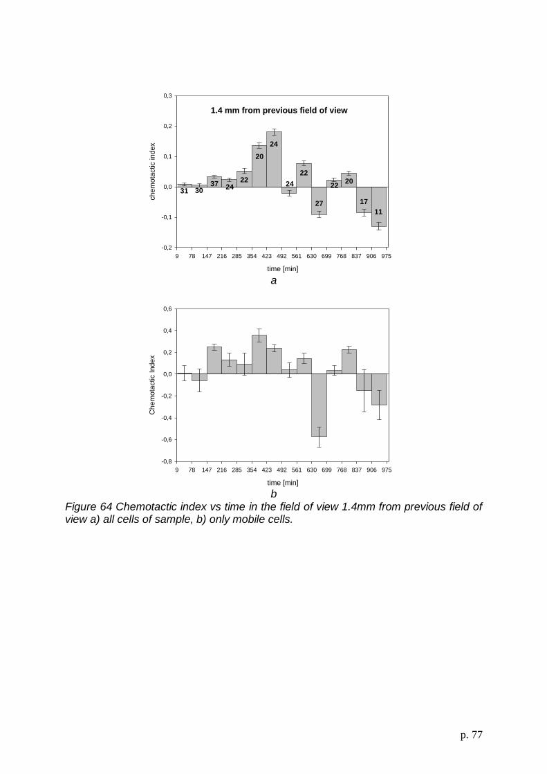
p. 77

1.4 mm from previous field of view

time [min]

9 78 147 216 285 354 423 492 561 630 699 768 837 906 975

chem

ota

ctic index

-0,2

-0,1

0,0

0,1

0,2

0,3

31 3037 24

22

20

24

24

22

27

2220

17

11

a

time [min]

9 78 147 216 285 354 423 492 561 630 699 768 837 906 975

Chem

ota

ctic Index

-0,8

-0,6

-0,4

-0,2

0,0

0,2

0,4

0,6

b

Figure 64 Chemotactic index vs time in the field of view 1.4mm from previous field of view a) all cells of sample, b) only mobile cells.

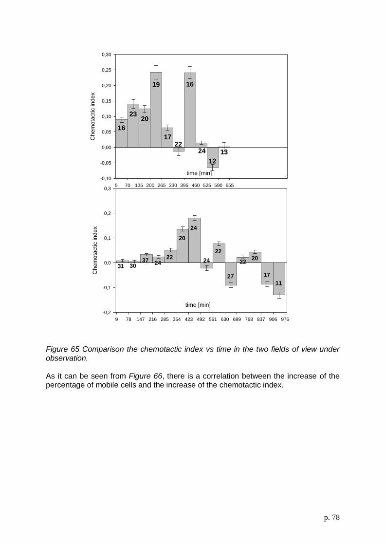
p. 78

time [min]

9 78 147 216 285 354 423 492 561 630 699 768 837 906 975

Ch

em

ota

ctic in

de

x

-0,2

-0,1

0,0

0,1

0,2

0,3

31 3037 24

22

20

24

24

22

27

2220

17

11

time [min]

5 70 135 200 265 330 395 460 525 590 655

Ch

em

ota

ctic in

de

x

-0,10

-0,05

0,00

0,05

0,10

0,15

0,20

0,25

0,30

13

1722

16

12

24

19

2023

16

Figure 65 Comparison the chemotactic index vs time in the two fields of view under observation. As it can be seen from Figure 66, there is a correlation between the increase of the percentage of mobile cells and the increase of the chemotactic index.

p. 79

time [min]

0 100 200 300 400 500 600 700

Fra

ctio

n o

f ce

lls m

ob

ile

0,00

0,05

0,10

0,15

0,20

0,25

0,30

a

time [min]

0 200 400 600 800 1000

Fra

ction o

f cells

mobile

0,05

0,10

0,15

0,20

0,25

0,30

0,35

0,40

b

Figure 66 Fraction of mobile cells vs time in field of view near the wall (a)and in the field of view far from the wall (b). As known from the literature, cell motility is associated with elongation of the cell body in the direction of motion (cell polarization). The extent of cell polarization has been quantified in terms of the ratio between the major and minor axis of the cell body. Figure 67 illustrates the increase of cell polarization with chemotatic index. It can also be noticed that the axis ratio of the mobile cells is higher compared to that of the whole population due to to rounded shape exhibited by immobile cells.

p. 80

time [min]

200 400 600 800 1000

Ra

tio

of a

xis

ce

lls

1,2

1,4

1,6

1,8

2,0

2,2

2,4

2,6

2,8

3,0

3,2

Average Time vs Ratio of cell axis

Average Time vs Ratio of cell mobile axis

Figure 67 Ratio between the major and minor axis of Jurkat cells vs time (red line: mobile cells, blu line: immobile cells.

5 mm from the membrane

time [min]

5 78 151 224 297 370

Ch

em

ota

ctic in

de

x

-0,5

-0,4

-0,3

-0,2

-0,1

0,0

0,1

0,2

a

p. 81

time [min]

5 78 151 224 297 370

Ch

em

ota

ctic ind

ex o

f m

ob

ile c

ells

mo

bile

-0,4

-0,2

0,0

0,2

0,4

0,6

b

Figure 68 Chemotactic index vs time for Jurkat cell (SDF 1nm) a) all cells, b) only mobile cells. Compared to previous experiments, a lower value of the chemotactic index was observed likely due to a smaller fraction of mobile cells. In Figure 69 the chemotactic index for Jurkat cell without chemoattractant is plotted as a function of time. As the plot shows, the chemotactic index fluctuates around zero, thus indicating random cell motility.

time[min]

100 200 300 400 500

Ch

em

ota

tic index

-0,2

-0,1

0,0

0,1

0,2

0,3

(5)

(1)

(5)(4)

(0)

(3)

(0)

5342

3949

27

29

50

Figure 69 Chemotactic index vs time for Jurkat cell without chemoattractant A direct analysis of cell trajectories allows one to detect a different cell behavior in presence or absence of chemoattractant. In fact, the motion of cells in the xy plane is random (random motion) in the absence of chemoattractant (Figure 70a), while it is directed towards the chemoattractant source (Figure 70b) in the presence of a concentration gradient.

p. 82

x [micron]

-150 -100 -50 0 50 100 150

y [m

icro

n]

-150

-100

-50

0

50

100

150

200

a

x [micron]

-120 -100 -80 -60 -40 -20 0 20 40 60 80

y [m

icro

n]

-80

-60

-40

-20

0

20

40

b

Figure 70 Trajectories of Jurkat cells a) in absence of chemoattractant, b) with chemoattractant

4.2 Fibrosarcoma cells

In this case FBS was used as a chemoattractant, Data analysis was perfromed in the same way as previously described for Jurkat cells. Figure 71 shows the chemotactic index vs time for fibrosarcoma cells, in two fields of view at a distance from the membrane of 5mm and 10mm, respectively.

p. 83

time [min]

0 200 400 600 800

Chem

ota

tic index

-0,2

-0,1

0,0

0,1

0,2

0,3

26

29

28

2930 26

22

20

(2)

(2)

(6)

(1)

(3)(1)

(0)

(3)

5 mm from the membrane

a

time [min]

0 200 400 600 800 1000 1200 1400

Ch

em

ota

ctic in

de

x

-0,15

-0,10

-0,05

0,00

0,05

0,10

0,15

40

4241

3942

4140

46

39 29

23

(3)

(4)

(2)(2)

(4)

(4)

(3)

(1)

(4)(2)

(2)

10 mm from the membrane

b

Figure 71 Chemotactic index vs time for fibrosarcoma cells, a) 5mm from the membrane, b) 10mm from the membrane. The percentage of mobile cells is equal to 46% in the first field of view and 55% in the second one. In the field of view at 5mm from the membrane the cell response to FBS is greatest in two time intervals: between 216 and 322 minutes (I = 0.21) and between 746 and 852 minutes (I = 0.26). In the field of view at 10 mm from the membrane, the chemotactic index is highest in the range between 1028 and 1142 minutes and is equal to 0.11. The elongation of the cell body in the direction of the membrane up to the gradient of chemoattractant concentration (cell polarization) can be seen in Figura72a. Figura72b shows the major axis between the fibrosarcoma cells and the normal to the membrane. Figura72c-d shows the distributions of the angle between major axis of cells and the normal to the membrane in the random (c) and directional motility (d) case. For

p. 84

fibroblasts and other tissue cells with much slower migration speed than Jurkat cells the chemotactic cell response is more significantly quantified in terms of cell polarization and orientation as compared to the chemotactic index.

a b

c d

Figura72 a) Optical image of fibrosarcoma cells oriented in the direction of the membrane, b) major axis of fibrosarcoma cells and the normal to the membrane c) distribution of the angle between major axis of cells and the normal to the membrane under random motility conditions (no chemoattractant) d) distribution of the angle between major axis of cells and the normal to the membrane in a chemotaxis experiment.

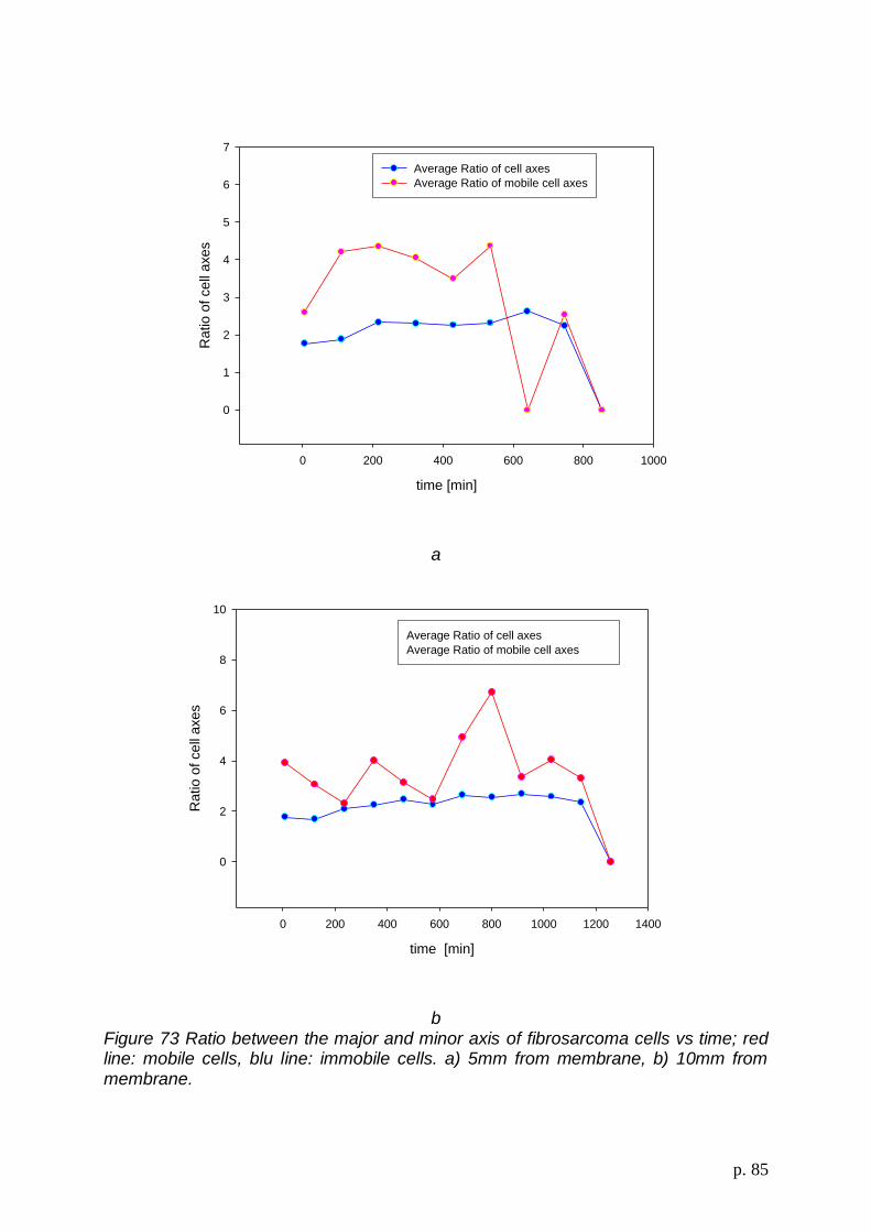
p. 85

time [min]

0 200 400 600 800 1000

Ratio

of cell

axes

0

1

2

3

4

5

6

7

Average Ratio of cell axes

Average Ratio of mobile cell axes

a

time [min]

0 200 400 600 800 1000 1200 1400

Ra

tio

of ce

ll axe

s

0

2

4

6

8

10

Average Ratio of cell axes

Average Ratio of mobile cell axes

b

Figure 73 Ratio between the major and minor axis of fibrosarcoma cells vs time; red line: mobile cells, blu line: immobile cells. a) 5mm from membrane, b) 10mm from membrane.

p. 86

In a second experiment the trend of the average chemotactic index was similar to that of the first one. In the time interval between 230 and 340 minutes the chemotactic index attains the maximum value of 0.14 (Figure 46).

time [min]

11 120 230 340 450 560

Che

mo

tactic ind

ex

-0,10

-0,05

0,00

0,05

0,10

0,15

0,20

48

46

37

34

28

(2)

(3)

(6)(5)

(5)

Figure 74 Chemotactic index vs Time for fibrosarcoma cell (FBS)

4.3 Lymphocyte Mononuclear cells

Mononuclear white blood cells were purified from peripheral blood from healthy human volunteers by using density gradient centrifugation. The preparation of the sample was carried out as previously described for the other cell cultures. In all experiments the SDF chemokine at the concentration of 4.5 nM was used. The first experiment was run on the same day that the cells were purified. The cell response to the gradient of SDF was not high as in the other cases. Moreover, the concentration of cells was low and the percentage of mobile cells was 24%. Figura 75 shows that the maximum value of index I (= 0.17) was reached during the period between 110 and 164 minutes. In the second experiment two different fields of view were chosen: one at 3.57 mm and the other at 9.85 mm from the membrane. In the first field (Figura 76a), the percentage of mobile cells was 58%, and the highest value of the chemotactic index is observed in between 41 and 78 minutes and is equal to 0.26. In the second field of view the percentage of mobile cells is 67%, and the highest value of the chemotactic index was recorded in the range between 690 and 743 minutes and is equal to 0.23 (Figura 76b).

p. 87

time [min]

56 110 164 218 272 326

Ch

em

ota

ctic ind

ex

-0,4

-0,3

-0,2

-0,1

0,0

0,1

0,2

0,3

38

37

40

37 30

(4)

(7)

(8)

(4) (6)

Figura 75 Chemotactic index vs time for lymphocyte cells (SDF 4.5 nm)

time [min]

4 41 79 117 154 192 229 267

Chem

ota

ctic index

-0,10

-0,05

0,00

0,05

0,10

0,15

0,20

0,25

0,30

96

90

91

83

75

6863

(37)

(28)

(18)

(17)

(7)(8) (13)

3.57 mm from the membrane

a

time [min]

427 479 532 585 638 691 743 796 849 902 955 10071060111311661219

Chem

ota

ctic index

-0,2

-0,1

0,0

0,1

0,2

0,3

96

8775

77

86

66

82

7087

69

59

57 55

95

94

(30)

(19)

(20)(18)

(16)

(8)

(19)

(13) (16)

(22)

(28)

(36)

(22)

(22) (12)

9.85 mm from the membrane

b

Figura 76 Chemotactic index vs time for lymphocyte cells, a) field of view at 3.57mm from the membrane, b) field of view at 9.85mm from the membrane.

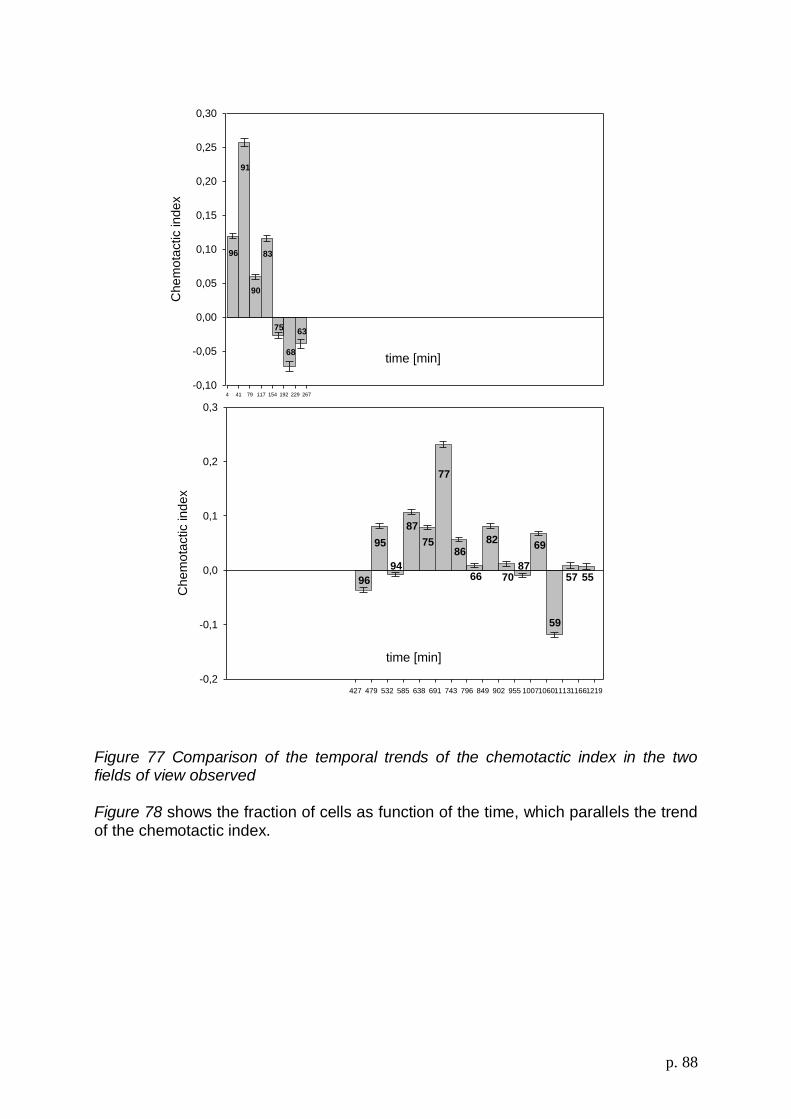
p. 88

time [min]

4 41 79 117 154 192 229 267

Chem

ota

ctic index

-0,10

-0,05

0,00

0,05

0,10

0,15

0,20

0,25

0,30

96

90

91

83

75

68

63

time [min]

427 479 532 585 638 691 743 796 849 902 955 10071060111311661219

Chem

ota

ctic index

-0,2

-0,1

0,0

0,1

0,2

0,3

96

87

75

77

86

66

82

7087

69

59

57 55

95

94

Figure 77 Comparison of the temporal trends of the chemotactic index in the two fields of view observed Figure 78 shows the fraction of cells as function of the time, which parallels the trend of the chemotactic index.

p. 89

time [min]

0 50 100 150 200 250

Fra

ction

of ce

lls m

ob

ile

0,05

0,10

0,15

0,20

0,25

0,30

0,35

0,40

0,45

a

time [min]

200 400 600 800 1000 1200 1400

Fra

ctio

n o

f ce

lls m

ob

ile

0,05

0,10

0,15

0,20

0,25

0,30

0,35

0,40

0,45

b

Figure 78 The fraction of mobile cells as a function of time. a) field of view at 3.57mm from the membrane, b) field of view at 9.85mm from the membrane. In the third experiment a field of view at 5 mm from the membrane was analyzed. As it can be seen from Figure 79, the chemotactic index reaches two maximum values between 146 and 192 minutes (I = 0.15) and between 284 and 330 minutes (I = 0.15).

p. 90

time [min]

9 55 101 147 192 238 284 330

Chem

ota

ctic index

-0,15

-0,10

-0,05

0,00

0,05

0,10

0,15

0,20

148

106

124

102

100

95

90

(59) (37)

(23)

(20)

(14)

(13)

(11)

Figure 79 Chemotactic index vs time for lymphocyte cells (the field of view is at 5mm from the membrane).

Figure 80 illustrates the comparison between the chemotactic index and the specific gradient. The yellow highlighted region shows that the maximum chemotactic index corresponds to the highest specific concentration gradients. When the spatial CF concentration gradient decays, the cell response to the chemoattractant vanishes as well.

p. 91

Figure 80 Comparison between the chemactic index and the specific gradient.

p. 92

5 Conclusion

The main purpose of this study is to describe an in vitro chemotaxis assay for Jurkat and slow moving fibroblast-like cells. The assay is carried out in a tissue-equivalent collagen or fibrin gel so that, unlike other chemotaxis assays from literature, the cell behavior is observed in a physiologically relevant environment. (The benefits of direct cell tracking and imaging of the CF concentration gradient follow from the optically transparency of these gels). This requires that a sufficiently steep CF concentration gradient is maintained over many hours, since a typical speed for tissue cells in these gels is less than one cell diameter per hour. To study chemoattractant diffusion a fluorescently labeled dextran was used (FITC-dextran). The FITC-dextran selected for the experiments has a molecular weight comparable to that of the chemoattractants investigated, so that a similar diffusion behavior can be assumed. We have shown that geometrical constraint of FITC-dextran diffusion through collagen gel using our assay chamber and consequent maintenance of a sufficiently steep concentration gradient over 24 h enables significant chemotactic migration of cells. Since collagen fibrils can become aligned near a surface as the gel forms or within the gel as it compacts due to traction exerted by entrapped cells, the possible contributions of contact guidance needed to be considered. Restricting measurements to regions of the gel at least 1 mm from surfaces mitigated any surface induced alignment effects and using low cell concentrations prevented any significant gel compaction during the 24-h observation period. The absence of any contact guidance due to these effects was supported by the random cell orientation results obtained in control sample without chemoattractants. This was also supported by polarized light microscopy examination of the gel region analyzed for cell alignment after the observation period, which did not show a significant or systematic birefringence pattern in the bulk of the gel In order to validate the proposed assay experiments were performed on three different cell lines. Cell behavior is characterized by calculating two key parameters: the mean square displacement and the chemotactic index. IThe maximum value of the chemotactic index was found to be associated with the highest values of the concentration specific gradient. When the spatial CF concentration gradient decays, the cell response to the chemoattractant vanishes as well. As known from the literature, cell motility is associated with elongation of the cell body in the direction of motion (cell polarization). The extent of cell polarization has been quantified in terms of the ratio between the major and minor axis of the cell body. For fibroblasts and other tissue cells with much slower migration speed than Jurkat cells the chemotactic cell response is more significantly quantified in terms of cell polarization and orientation as compared to the chemotactic index.

p. 93

BIBLIOGRAPHY

[1]. Laurencin, C. T., et al., Tissue engineering: Orthopedic applications Annu. Rev. Biomed. Eng. (1999) 1, 19

[2]. Ma, P. X., and Zhang, R., J. Synthetic nano-scale fibrous extracellular matrix Biomed. Mater. Res. (1999) 46, 60

[3]. Fertala, A., et al., J. Biomed. Mapping critical sites in collagen II for rational design of gene-engineered proteins for cell-supporting materials Mater. Res. (2001) 57, 48

[4]. Murthy, N., et al., J. Control. Design and synthesis of pH-responsive polymeric carriers that target uptake and enhance the intracellular delivery of oligonucleotides Release (2003) 89, 365-374

[5]. Murthy, N., et al., oinspired pH-responsive polymers for the intracellular delivery of biomolecular drugs Bioconjugate Chem. (2003) 14, 412-419

[6]. Gibson, P., et al., Transport properties of porous membranes based on electrospun nanofibers Colloid Surf. A (2001) 187-188, 469

[7]. Ramakrishna, S., et al., unpublished results

[8]. Formhals, A. US Patent 1975504, 1934.

[9]. Formhals, A. US Patent 2160962, 1939.

[10]. Formhals, A. US Patent 2187306, 1940.

[11]. Taylor, G. I. Proc Roy Soc London 1969, A313, 453.

[12]. Buchko, C. J.; Chen, L. C.; Yu, S.; Martin, Processing and Microstructural Characterization of Porous Biocompatible Protein Polymer Thin Films D. C. Polymer 1999, 40, 7397.

[13]. Baumgarten, P. K. J Electrostatic Spinning of Acrylic MicrofibersColloid Interface Sci 1971, 36, 71.

[14]. Larrondo, L.; R. St.Mandley, Electrostatic fiber spinning from polymer melts. III. Electrostatic deformation of a pendant drop of polymer melt Polym Sci: Polymer Physics Edn 1981, 909.

[15]. Larrondo, L.; R. St. J. J Mandley, Electrostatic fiber spinning from polymer melts. II. Examination of the flow field in an electrically driven jet Polym Sci: Polymer Physics Edn 1981, 921.

[16]. Hayati, I.; Bailey, A. I.; Tadros, T. F. J Investigation into the mechanism of electrohydrodynamic spraying of liquids, I. Effect of electric field the environment on pendant drops and factors affecting the formation of stable jets and atomisationColloid Interface Sci 1987, 117, 205-221

[17]. Doshi, J.; Reneker, D. H. J Elec-trospinning process and application of electro-spun fibers Electrostatics 1995, 35, 151.

[18]. Jaeger, R.; Bergshoef, M. M.; Batlle, C. M. I.; Holger, S.; Vancso, G. J. Electrospinning of Ultra-Thin Polymer Fibers Macromol Symp 1998, 127, 141.

p. 94

[19]. Deitzel, J. M.; Kleinmeyer, J.; Harris, D.; BeckTan, The effect of processing variables on the morphology of electrospun nanofibres and textilesN. C Polymer 2001, 42, 261.

[20]. Deitzel, J. M.; Kleinmeyer, J. D.; Hirvonen, J. K.; BeckTan, Controlled deposition of electrospun poly (ethylene oxide) fibres N. C Polymer 2001, 42, 8163.

[21]. Warner, S. B.; Buer, A.; Grimler, M.; Ugbolue, S. C.; Rutledge, G. C.; Shin, M. Y. National Textile Center Annu Report November 1998, 83.

[22]. Moses, M.; Hohman, M. M.; Shin, Y. M.; Rutledge, G. C.; Brenner, M. P. Electrospinning and electrically forced jets. I. Stability theory Phys Fluids 2001, 13, 2201.

[23]. Reneker, D.H., Chun, I. (1996), "Nanometre diameter fibres of polymer produced by electrospinning", Nanotechnology, Vol. 7 No.3, pp.216-23.

[24]. Shin, Y. M.; Hohman, M. M.; Brenner, M. P.; Rutledge, G. C. Experimental characterization of electrospinning.the electrically forced jet and instabilities Polymer 2001, 42, 9955.

[25]. Spivek, A. F.; Dzenis, Y. A. Inst Penn Conf 1999, 163, 175.

[26]. Gibson, P. W.; Gibson, H. L.; Rivin, Electrospun fiber mats: Transport properties D. AIChe J 1999, 45, 190.

[27]. Raleigh, X. L. Philosophical Magazine, 1884, 44, 184.

[28]. Zeleny, J. Instability of Electrified Liquid Surfaces Phys Rev 1917, 10, 1.

[29]. Yarin, A. L.; Koombhongse, S.; Reneker, D. H. J Bending instability in electrospinning of nanofibers Appl Phys 2001, 89, 3018.

[30]. Cloupeau, M.; Prunet-Foch, B. Electrostatic spraying of liquids: main functional modes J of Electrostatics 1990, 25, 165.

[31]. Grace, J. M.; Marijnissen, J. C. M. A review of liquid atomization by electrical means J of Aerosol Science 1994, 25, 1005.

[32]. Shin, Y. M.; Hohman, M. M.; Brenner, M. P.; Rutledge, G. C. Electrospinning: a whipping fluid jet generates submicron polymer Appl Phys Lett 2001, 78, 1149.

[33]. Darby, R. Viscoelastic Fluids An Introduction to Their Properties and Behaviour ; Marcel Dekker: New York, 1976.

[34]. Yarin, A. L. Free Liquid Jets and Films: Hydrodynamics and Rheology; Longman: New York, 1993.

[35]. Spivak, A. F.; Dzenis, Y. A.; Reneker, D. H. A Model of Steady State Jet in the Electrospinning Process Mechanics Research Communications 2001, 27, 37.

[36]. Reneker, D. H.; Yarin, A. L.; Fong, H.; Koombhongse, S. Bending instability of electrically charged liquid jets of polymer solutions in electrospinning. J Appl Phys 2000, 87, 4531.

[37]. Jeans, J. The mathematical Theory of Electricity and Magnetism; Cambridge University Press, 1958.

[38]. Buer, A.; Ugbolue, S. C.; Warner, S. B. Electrospinning and Properties of some Nanofibers Textile Research Journal 2001, 71, 323-328.

p. 95

[39]. Megelski, S.; Stephens, J. S.; Chase, D. B.; Rabolt, J. F Arrays of Micro- and Nanopores on Electrospunn Polymer Fibers. Macromolecules 2002, 35, 8456.

[40]. Srinivasarao, M.; Collings, D.; Philips, A.; Patel, S. Three-Dimensionally Ordered Array of Air Bubbles in a Polymer Film Science 2001, 292, 79.

[41]. Zong, X. H.; Kim, K.; Fang, D. F.; Ran, S. F.; Hsiao, B. S.; Chu, B. Structure and process relationship of electrospun bioabsorbable nanofiber membranes Polymer 2002, 43, 4403.

[42]. Fridrikh, S. V.; Yu, J. H.; Brenner, M. P.; Rutledge, G. C. Controlling the Fiber Diameter during Electrospinning Physical Review Letters, 2003, 90, 144502.

[43]. Bognitzki, M.; Czado, W.; Frese, T.; Schaper, A.; Hellwig, M.; Steinhart, M.; Greiner, A.; Wendorff, H. Nanostructured Fibers via Electrospinning Adv Mater 2001, 13, 70.

[44]. Lee, K. H.; Kim, H. Y.; La, Y. M.; Lee, D. R.; Sung, N. H. Influence of a mixing solvent with tetrahydrofuran and N,N-dimethylformamide on electrospun poly(vinyl chloride) nonwoven mats J Polym Sci: Part B: Polymer Physics 2002, 40, 2259.

[45]. Reneker, D. H.; Chun, I Nanometre diameter fibres of polymer, produced by electrospinning. Nanotechnology 1996, 7, 216-223

[46]. Matthews JA,Bowlin GL. Electrospinning of collagen nanofibers Biomacromolecules 2003(2):232-8

[47]. Bose, G. M. Recheres sur la cause et sur la veritable theorie del'electricite: Wittenberg, 1745.

[48]. Li D, Wang Y and Xia Y 2003 Electrospinning of polymeric and ceramic nanofibers as uniaxially aligned arrays Nano Lett. 3 1167

[49]. Li D, Wang Y and Xia Y 2004 Electrospinning nanofibers as uniaxially aligned arrays and layer-by-layer stacked films Adv. Mater. 16 361

[50]. Xu CY, Yang F, Wang S, Ramakrishna S. In vitro study of human vascular endothelial cell function on materials with various surface roughness. J Biomed Mater Res 2004;71A(1): 154–61.

[51]. Xu CY, Inai R, Kotaki M, Ramakrishna S. Aligned biodegradable nanofibrous structure: a potential scaffold for blood vessel engineering. Biomaterials 2004;25(5):877–86.

[52]. Yang F, Xu CY, Kotaki M, Wang S, Ramakrishna S. Characterization of neural stem cells on electrospun poly(L-lactic acid) nanofibrous scaffold. J Biomater Sci Polym Ed, in press.

[53]. Engelberg I, Kohn J. Physico-mechanical properties of degradable polymers used in medical applications: a comparative study. Biomaterials, 12(3), 292-304, 1991

[54] Sutherland FW, Perry TE, Yu Y, Sherwood MC, Rabkin E, Masuda Y, Garcia GA, McLellan DL, Engelmayr GC Jr, Sacks MS, Schoen FJ, Mayer JE Jr. From stem cells to viable autologous semilunar heart valve. Circulation, 111(21), 2783-91, 2005

p. 96

[55] Jones DS, Djokic J, McCoy CP, Gorman SP. Poly(epsilon-caprolactone) and poly(epsiloncaprolactone)-polyvinylpyrrolidone-iodine blends as ureteral biomaterials: characterisation of mechanical and surface properties, degradation and resistance to encrustation in vitro. Biomaterials, 23(23), 4449-58, 2002

[56] Averous L, Moro L, Dole P, Fringant C. Properties of thermoplastic blends: starch-polycaprolactone. Polymer, 41, 4157–67, 2000

[63] Pitt CG. Poly-caprolactone and its copolymers. Biodegradable Polymers as Drug Delivery Systems (New York: Dekker) 71–119, 1990

[57] Yoshimoto H, Shin YM, Terai H. A biodegradable nanofiber scaffold by electrospinning and its potential for bone tissue engineering. Biomaterials, 24(12), 2077-82, 2003

[56] Hutmacher DW, Schantz T, Zein I, Ng KW, Teoh SH, Tan KC. Mechanical properties and cell cultural response of polycaprolactone scaffolds designed and fabricated via fused deposition modeling. J Biomed Mater Res, 55(2), 203-16, 2001

[57] Ciapetti G, Ambrosio L, Savarino L, Granchi D, Cenni E, Baldini N, Pagani S, Guizzardi S, Causa F, Giunti A. Osteoblast growth and function in porous poly epsilon -caprolactone matrices for bone repair: a preliminary study. Biomaterials, 24(21), 3815-24, 2003

[58] Sung HJ, Meredith C, Johnson C, Galis ZS. The effect of scaffold degradation rate on three-dimensional cell growth and angiogenesis. Biomaterials, 25(26), 5735-42, 2004

[59] Htay AS, Teoh SH, Hutmacher DW. Development of perforated microthin poly(epsilon-caprolactone) films as matrices for membrane tissue engineering. J Biomater Sci Polym Ed, 15(5), 683-700, 2004

[60] Laurent, T. C. Chemistry and Molecular Biology of the Intercellular Matrix; Academic: New York, 1970.

[61] Balazs, E. A.; Denlinger, J. L. The Eye; Academic: New York, 1984.

[62] Lapcik, L., Jr.; Lapci, L.; Smedt, S. D.; Demeester, J. Chem. ReV. 1998, 98, 2663-84.

[63] Goa, K. L.; Benfield, P. Drugs 1994, 47, 536-66.

[64] Junxing Li,1 Aihua He,*1 Charles C. Han,*1 Dufei Fang,2 Electrospinning of Hyaluronic Acid (HA) and HA/Gelatin Blends. Macromolecular, 10.1002/marc.200500726

[65] In Chul Um,† Dufei Fang,‡ Benjamin S. Hsiao,† Akio Okamoto Electro-Spinning and Electro-Blowing of Hyaluronic Acid. Biomacromolecules 2004, 5, 1428-1436

[66] Shalaby SW, Johnson A. In: Shalaby SW, editor. Biomedical polymer. Designed to degrade systems. Munich: Carl Hanser Verlag; 1994. p. 1–34.

[67] Dunn RL. In: Hollinger JO, editor. Biomedical applications of synthetic biodegradable polymers. Boca Raton, FL: CRC Press; 1995. p. 17–31

p. 97

[68] Grande DA, Halberstadt C, Naughton G, Schwartz R, Manji R. Evaluation of matrix scaffolds for tissue engineering of articular cartilage grafts. J Biomed Mater Res 1997;34:211–20.

[69] Aigner J, Tegeler J, Hutzler P, Campoccia D, Pavesio A, Hammer C, Kastenbauer E, Naumann A. Cartilage tissue engineering with novel nonwoven structured biomaterial based on hyaluronic acid benzyl ester. J Biomed Mater Res 1998;42:172–81.

[70] Bhat GS. Nonwovens as three-dimensional textiles for composites. Mater Manuf Process 1995;10:667–88.

[71] Ma T, Li Y, Kniss DA, Yang ST. Tissue engineering human placenta trophoblast cells in 3-D fibrous matrix: spatial effects on cell proliferation and function. Biotechnol Prog 1999;15: 715–24.

[72] Organ GM, Vacanti JP. Tissue engineering neointestine. In: Lanza RP, Langer R, Chick WL, editors. Principles of tissue engineering. Austin, TX: Academic Press; 1997. p. 441.

[73] Fogh, J.M., Orfeo, T., 1977. One hundred and twenty seven cultured human tumor cell lines producing tumors in nude mice. J. Natl. Cancer Inst. 59: 221-226.

[74] Braun, A., Hämmerle, S., Suda, K., Rothen-Rotishauser, B., Günther, M., Krämer, S., Wunderli-Allenspach, H., 2000. Cell cultures as tools in biopharmacy. Eur. J. Pharm. Sci. 11, S51-S60.

[75] Pinto, M., Robine-Leon, S., Appay, M.-D., Kedinger, M., Triadou, N., Dussaulx, E., Lacroix, B., Simon-Assmann, P., Haffen, K., Fogh, J., Zweibaum, A., 1983. Enterocyte-like differentiation and polarization of the human colon carcinoma cell line Caco-2 in culture. Biol. Cell 47: 323-330.

[76] Artursson, P.,1990. Epithelial transport of drugs in cell culture. I: A model for studying the passive diffusion of drugs over intestinal absorptive (Caco-2) cells. J. Pharm. Sci. 79: 476-482.

[77] Artursson, P., Borchardt, R.T., 1997. Intestinal drug absorption and metabolism in cell cultures: Caco-2 and beyond. Pharm. Res. 14: 1655-1658.

[78] Yonezawa, T.; Imamura, K.; Kimizuka, N. Langmuir 2001, 17, 4701-4703.

[79] Bonnemann, H.; Brijoux, W.; Brinkmann, R. J. Mol. Catal. 1994, 86, 129-134.

[80] Horswell, S.; Schiffrin, D. J. J. Am. Chem. Soc. 1999, 121, 5573-5578.

[81] Itoh, H.; Naka, K.; Chujo, Y. Polym. Bull. (Berlin) 2001, 46, 357-362.

[82] Hirai, H.; Yakaru, N. I.; Seta, Y.; Hodosima, S. React. Funct. Polym. 1998, 37, 12-131.

[83] Clark, R. A. F. (1996). Wound repair: overview and general considerations. In “The Molecular and Cellular Biology of Wound Repair” (R. A. F. Clark, Ed.), 2nd ed., pp. 3-35, Plenum, New York.

[84] Reddi, A. H. (1997). Bone morphogenetic proteins: An unconventional approach to isolation of first mammalian morphogens. Cytokine Growth Factor Rev. 8,11–20.

p. 98

[85] Mutsaers, S. E., Bishop, J. E., McGrouther, G., and Laurent, G. J. (1997). Mechanisms of tissue repair: From wound healing to fibrosis. Int. J. Biochem. Cell Biol. 29, 5–17.

[86] McCarthy, J. B., Iida, J., and Furcht, L. T. (1996). Mechanisms of parenchymal cell migration into wounds. In “The Molecular and Cellular Biology of Wound Repair” (R. A. F. Clark, Ed.), 2nd ed., pp. 373–390, Plenum, New York.

[87] Moghe, P. V., Nelson, R. D., and Tranquillo, R. T. (1995). Cytokine-stimulated chemotaxis of human neutrophils in a 3-D conjoined fibrin gel assay. J. Immunol. Methods 180, 193–211.

[88] Boyden, S. (1962). The chemotactic effect of mixtures of antibody and antigen on polymorphonuclear leucocytes. J. Exp. Med. 115, 453–466.

[89] Noble, P. B. (1987). Extracellular matrix and cell migration: Locomotory characteristics of MOS-11 cells within a threedimensional hydrated collagen lattice. J. Cell Sci. 87, 241–248.

[90] Zicha, D., Dunn, G. A., and Brown, A. F. (1991). A new directviewing chemotaxis chamber. J. Cell Sci. 99, 769–775.

[91] Tomasek, J. J., and Hay, E. D. (1984). Analysis of the role of microfilaments and microtubules in acquisition of bipolarity and elongation of fibroblasts in hydrated collagen gels. J. Cell Biol. 99, 536–549.

[92] Shi, W., Kohler, T., and Zusman, D. R. (1993). Chemotaxis plays a role in the social behaviour of Myxococcus xanthus. Mol. Microbiol. 9, 601–611.

[93] Long, M. M., King, V. J., Prasad, K. U., and Urry, D. W. (1987). Cell attachment and chemotaxis can utilize the same peptide sequence of fibronectin. Biochim. Biophys. Acta 928, 114–118.

[94] Freshney, R. I. (1987). “Culture of Animal Cells: A Manual of Basic Technique,” A. R. Liss, New York.

[95] David M. Knapp, Emelie F. Helou, and Robert T. Tranquillo1A Fibrin or Collagen Gel Assay for Tissue Cell Chemotaxis: Assessment of Fibroblast Chemotaxis to GRGDSP Experimental Cell Research 247, 543–553 (1999)

[96] Modis, L. (1991). “Organization of the Extracellular Matrix: A Polarization Microscopy Approach,” CRC Press, Boca Raton, FL.

[97]. Tranquillo, R. T. (1998). Self-organization of tissue-equivalents: the nature and role of contact guidance. In “Cell Behaviour: Control and Mechanism of Motility” (J. Lackie, G. Dunn, and G. Jones, Eds.), pp. 27–42, Portland Press, Oxford.

[98]. Stopak, D., and Harris, A. K. (1982). Connective tissue morphogenesis

by fibroblast traction. Dev. Biol. 90, 383–398.

p. 99

Appendix

Publications

S. Caserta, L. Sabetta, M. Simeone and S. Guido, “Shear-induced coalescence in aqueous biopolymer mixtures”, Chem. Eng. Sci., 60, 1019-1027 (2005)

Conferences

The work of this PhD has been presented at the following international conferences.

L. Sabetta, S. Caserta, V. Sibillo, M. Simeone, S. Guido “Time-Lapse Imaging and 3D Cell Tracking by Computer-Controlled Video Microscopy. Applications to Chemotaxis”. AIChE annual meeting Salt Lake City, UT November 4 - 9, 2007

F. Raffone, L. Sabetta, S. Caserta, V. Sibillo, M. Simeone and S. Guido “Time-lapse imaging and 3d cell tracking by computer controlled video microscopy. Applications to chemotaxis.”. Focus on Microscopy 2007 10 – 13 April 2007 Valencia, Spain

S. Guido, L. Sabetta, F. Raffone, S. Caserta, V. Sibillo, M. Simeone “Time-lapse imaging and 3D cell tracking by computer-controlled video microscopy. Applications to chemotaxis.” ELSO 1-4 September 2007 Dresden, Germany.

V. Sibillo, S. Caserta, L. Sabetta, M. Simeone, S. Guido, “Time-lapse imaging and 3D cell tracking by computer-controlled video microscopy applications to chemotaxis”, Cell Migration, Tissue Invasion and Disease. Embo Workshop October 2006

V. Sibillo, S. Caserta, L. Sabetta, M. Simeone, S. Guido, “A computer controlled microscope stage incubation system for time-lapse imaging of living cells applications to cell tracking”, Focus on Microscopy 2005, Jena (Germania), 20-23 marzo 2005

S. Caserta, L. Sabetta, M. Simeone and S. Guido, “Shear-induced coalescence in aqueous biopolymer mixtures”. Chemical Engineering Science 60 (2005), pp. 1019-1027.