Product Testing, Seller Disclosure and Certification∗

Jacopo Bizzotto†, Jesper Rudiger‡ and Adrien Vigier§

First Draft: September 2016This Draft: January 2018

Abstract

We study product certification by a certifier basing her decisions on a mixture of

information, some of which is voluntarily disclosed by the sellers, and some of which

she acquires first-hand by testing products. We determine the conditions under which

products are tested on the equilibrium path and show that when they are, then access

to cheaper and more accurate certifier tests can lower social welfare and certification

quality, by crowding out information disclosed by the sellers. Regulators may therefore

prefer to license certification to relatively inefficient certification agencies.

JEL classification: C72, D82, D83, G24, G28

Keywords: Certification, Product Testing, Information Acquisition, Information Disclosure

∗We thank Johannes Horner, Espen Moen, Pauli Murto, David Myatt, Marco Ottaviani, Vasiliki Skreta,

Juuso Valimaki, and Yanos Zylberberg for helpful discussions, and various seminar audiences for their com-

ments. All remaining errors are our own.†Department of Economics, University of Oslo. Email: jacopobi@econ.uio.no.‡Department of Economics, University of Copenhagen. Email: jesper.rudiger@econ.ku.dk.§Department of Economics, Norwegian Business School. Email: a.h.vigier@gmail.com.

1 Introduction

In many markets, certifiers must approve products before they can be sold. The long list

of products requiring approval in order to be commercialized includes drugs, cars, organic

products, pesticides, and sporting equipment. As sellers are typically better able than certifiers

to retrieve information about their own products, certifiers often rely on information that

sellers disclose voluntarily. However, to the extent that it can raise chances of approval, sellers

have a strategic incentive to conceal information. Certifiers therefore make their decisions

based on a mixture of information, some of which the certifiers acquire first-hand by testing

products. The European Commission Regulation 889/2008 laying down the rules for the

certification of organic products specifies for instance that

“sampling and analysing of products can be used as a supplementary tool to the verification of

documentary evidence with the aim to detect the use of non-authorised products or production

techniques.”

Similarly, the U.S. Food and Drug Administration (FDA) regularly acquires information on

top of what producers submit:1

“an FDA review team ... evaluates whether the studies the sponsor submitted show that the

drug is safe and effective ... Reviewers determine whether they need any additional information

... Sometimes, the FDA calls on advisory committees, who provide the FDA with independent

opinions and recommendations from outside experts on applications to market new drugs.”

The aim of the present paper is to shed light on the interplay between sellers’ voluntary

disclosure and a certifier’s information acquisition. We first determine the conditions in which

product testing actually materializes.2 If the certifier can pre-commit to a testing strategy or

if sellers are perfectly informed about products, then testing never occurs. By contrast, with

limited certifier commitment and imperfect information on the part of the sellers then – in

line with common practice in many markets – products are sometimes tested. We then show

that, in this case, cheaper and more accurate tests can induce lower social welfare and worse

1See the U.S. Food and Drug Administration website.2That is, we determine the conditions in which testing occurs on the equilibrium path.

1

certification quality, by crowding out information disclosed by the sellers.3

The analysis of our paper is foremost relevant for regulators in markets for certified prod-

ucts. In many markets, regulators delegate certification to independent certifiers. For example,

both the U.S. Department of Agriculture and the authorities in charge of the control system

for organic production in the E.U. leave the testing as well as the final decision as to whether

a food product qualifies as organic in the hands of independent accredited certifiers.4 Our

work shows among other things that, counter to intuition, regulators may find it optimal to

license certification to relatively inefficient certification agencies. We also examine whether

and how policies granting commitment power to certifiers can help improve social welfare and

certification quality. For instance, we find that regulators may benefit from imposing two

simple rules: rule one is not to test a product which the certifier would reject without a test;

rule two is to test any product which the certifier would approve without a test, but which

the certifier would reject if the product were to fail the test.

We construct a model comprising a buyer, a seller and a certifier. The seller owns a

product which can be good or bad. Whether the seller knows his product quality is private

information. A parameter α determines the probability with which the seller is informed. The

certifier’s goal is to approve (a product of) good quality and to reject bad quality. The seller

picks a signal to selectively disclose information to the certifier.5 After observing both the

signal selected and the outcome of this signal, the certifier chooses whether or not to perform

a noisy test.6 In case of approval, the seller sets a price and the buyer chooses whether or not

to buy. In case of rejection, the product cannot be sold.

The strategic interaction between the seller and the certifier works as follows. The seller

is of one of three types: informed that the product is good, informed that the product is

bad, or uninformed. The bad type always selects a signal chosen by at least one other type

of the seller. As testing is noisy, the good type selects a signal sufficiently informative to

avoid the test and ensure approval. The crux lies in the choice of the uninformed seller. The

uninformed would like to pool with the good type. However, as the good type selects a signal

more informative than the favorite signal of the uninformed seller, the latter must choose

3The quality of certification refers to the probability that a certifier certifies correctly, that is, eitherapproves a good product or rejects a bad product.

4For the list of certifiers accredited in the U.S. see the U.S. Department of Agricolture Certifier Locator.The European Commission provides the following list of approved control bodies:List of Control Bodies and Control Authorities in the Organic Sector.

5A signal is a garbling of the product quality, in the spirit of Kamenica and Gentzkow (2011).6The baseline model of Section 2 focuses on the case in which the certifier cannot pre-commit to a testing

strategy. Certifier commitment is examined in Section 4.

2

between pooling with the good type and selecting her own favorite signal: from his viewpoint,

the drawback of the second option is the negative impact on the certifier’s interim beliefs.7

As this drawback becomes more severe the greater the probability that the seller is informed,

when α is large only pooling equilibria exist. In particular, the product is never tested, and

improving the certifier’s product testing technology increases social welfare and certification

quality.

By contrast, when α is small, the uninformed seller separates from the good type for a

subset of product testing technologies, in which case product testing occurs with positive

probability. Specifically, the more accurate the test (or the cheaper the test), the harder for

the seller to obtain approval without facing the test in the first place. Better tests thus reduce

incentives for the uninformed to select a signal providing enough information to make testing

sub-optimal for the certifier. A trade-off therefore emerges: superior testing technologies

augment the amount of first-hand information available to the certifier, but reduce the amount

of information obtained from the seller. We show that, as a result, improving the certifier’s

testing technology can lower social welfare and certification quality.

Settings in which the seller is able to commit to a given signal before learning his type

constitute a special case of our model, corresponding to α = 0. The drug market appears to

be a good example of a market in which sellers commit in advance to information disclosed

about products (see, e.g., Kolotilin (2015)). More generally, the commitment setting seems

like a natural way to model markets in which sellers and certifiers interact repeatedly over

time, as is the case when sellers release periodically new versions of a product.

The related literature is discussed below. The baseline model is presented in Section 2.

Section 3 contains the core analysis and presents the main result. Section 4 studies the impact

of certifier commitment and explores various ways of improving social welfare and certification

quality. Section 5 extends the baseline model by adding noise to the information of the seller.

Section 6 concludes.

Related literature. We primarily contribute to the literature on certification, surveyed

in Dranove and Jin (2010). To the best of our knowledge, this paper is the first study of

the interplay between certifiers’ information acquisition and sellers’ voluntary disclosure. For

the most part, the literature on certification abstracts away from the problem of asymmetric

information between seller and certifier. In Lizzeri (1999) the certifier observes the type of

7The certifier’s interim beliefs refer to the certifier’s beliefs after observing the signal selected by the sellerbut before observing the outcome of this signal.

3

the seller but obfuscates this information in order to extract the full social surplus from

trade. Strausz (2005) relaxes the certifier’s commitment and studies the resulting problem of

dishonest certification. Stahl and Strausz (2017) examine the relative performance of “buyer

certification” vs. “seller certification”. In their setting, the certifier is committed to reveal

the type of the seller, but aims to maximize the profit made from selling her certificates. By

contrast, we study a certifier who chooses what information to obtain and who to certify, and

whose objective is to maximize social welfare. This appears to be in line with many markets

where certification services are provided by non-profit organizations.

Three papers are particularly related to ours: Perez-Richet and Skreta (2017), Quigley

and Walther (2017), and Henry and Ottaviani (2017). In Perez-Richet and Skreta (2017) the

certifier designs a test knowing that the seller can falsify results. Since the most accurate

test fails to be falsification proof, as in our setting the optimal test is partly inaccurate. The

mechanisms at play in the two models are however very different. There is no cheating in

our paper: the certifier sometimes prefers an inferior testing technology due to the fact that

better tests tend to crowd out information disclosed by the seller. Quigley and Walther (2017)

examine the impact of exogenous outside information on the seller’s voluntary disclosure. Our

setting differs from theirs in that we study the certifier’s choice to acquire information. This

feature in turn enables the seller to disclose information in order to manipulate the certifier’s

incentives to acquire information of her own. The two papers offer complementary views

regarding the danger of crowding out disclosure. However, crowding out operates through dif-

ferent mechanisms in the two settings: in Quigley and Walther (2017), as outside information

becomes more precise, a process of “reverse unraveling” unfolds whereby high-quality sellers

have stronger incentives to remain silent, thus increasing other sellers’ incentives to remain

silent too. Lastly, similar in spirit to what we do, Henry and Ottaviani (2017) examine the

quality of certification achieved under different forms of commitment.8 The central difference

with our paper is that in their model the seller fully controls the flow of information, whereas

in ours, the certifier can also acquire information.

We are also related to the recent literature on information design pioneered by Kamenica

and Gentzkow (2011). We contribute to this literature by introducing information acquisition

on the part of the receiver. Most of this literature assumes that the sender is the only source

8The authors show that granting commitment power to the seller maximizes the number of false positives(that is, the frequency with which bad products are approved) but eliminates false negatives (the frequencywith which good products are rejected); by contrast the no-commitment case minimizes the number of falsepositives but maximizes the number of false negatives; granting commitment power to the certifier induces anintermediate outcome, which Pareto dominates no commitment.

4

of information available to the receiver. Exceptions include Kolotilin (2016), Gentzkow and

Kamenica (2017) and Bizzotto, Rudiger and Vigier (2017). In Kolotilin (2016) the receiver is

privately informed; in Gentzkow and Kamenica (2017) multiple senders disclose information

to the receiver; in Bizzotto et al. (2017) the passing of time allows the receiver to observe

exogenous news. Finally, our paper is related to a small but growing literature on information

design with a privately informed sender, including Perez-Richet (2014), Alonso and Camara

(2014), ?, and ?.

2 Model

The broad features of the model are as follows. We consider a buyer, a seller (he), and a

certifier (she). The seller owns a product of uncertain quality, which the seller may or may

not know. The goal of the certifier is to approve good quality and to reject bad quality. The

certifier bases her decision on a mixture of information obtained by testing the product, and

disclosed voluntarily by the seller.

State of the World. The state of the world is (ω, τ) ∈ {G,B}×{g, u, b}: ω is the product

quality (either good or bad) and τ is the type of the seller, representing the latter’s private

information about ω. The seller of type g (resp. b) is privately informed that ω = G (resp.

ω = B). The seller of type u does not have any private information. The joint distribution of

(ω, τ) is common knowledge and given by

g u b

G ρα ρ(1− α) 0

B 0 (1-ρ)(1− α) (1-ρ)α

Thus (i) ω = G with probability ρ and (ii) (independently of the realization of ω) the seller

observes ω with probability α. We refer to ρ as the reputation of the seller and assume that

ρ ∈ (0, 12].9

Let Vω represent the buyer’s utility and V Sω the social value conditional on quality ω

being consumed. Thus V Sω > Vω (respectively V S

ω < Vω) captures positive (resp. negative)

consumption externalities. We focus on VG ≥ VB > 0 and V SG > 0 > V S

B ; other cases are

9The model is readily extended to higher values of the reputation, but at the cost of introducing morenotation.

5

trivial, we discuss them in the next subsection and relegate their analysis to Appendix F.

Lastly, we ease the exposition by setting V SG = 1 and V S

B = −1 (this restriction is relaxed in

Appendix F).

Information Disclosure and Product Testing. The seller can fully or partly disclose

information by choosing a signal π =(π(·|ω = G), π(·|ω = B)

), consisting of a pair of

conditional probability distributions π(·|ω = G) and π(·|ω = B) over a set of outcomes

S = {s1, s2}.10 Let Π denote the set of signals over S. The seller is allowed to choose any

signal in Π.

The certifier can perform a binary test of the product in order to retrieve information about

ω. The product testing technology is parameterized by (q, c). The parameter c ∈ (0,∞) is

the certifier’s cost of testing the product; q ∈ [12, 1] is the test accuracy: if ω = G then the

product passes the test with probability q and fails the test with probability 1 − q, whereas

if ω = B then the product passes the test with probability 1 − q and fails the test with

probability q. To keep the analysis tractable, whatever signal π the seller selects, the signal

outcome and the test result are assumed uncorrelated conditional on ω. Lastly, let η denote

an arbitrary positive real number, and T := {(q, c) : q − c ≥ 12

and q < 1 − η}. We assume

that the certifier’s technology belongs to T . Technologies outside T are either too expensive,

too accurate or too inaccurate to make the problem interesting; these cases are analyzed in

Appendix F.

Timing. The seller first observes his type, and then selects a signal. The certifier observes

the signal selected as well as the outcome of the signal and then chooses whether or not to

perform the test. After observing the test result, the certifier chooses between approval and

rejection. In case of rejection, the product cannot be sold. In case of approval, the seller sets

a price and the buyer chooses whether or not to buy. The buyer observes whether or not

the product is approved, but none of the earlier steps of the certification process. In case of

approval, the buyer also observes the price. Figure 1 summarizes the timing.

Payoffs. All players are risk-neutral. The seller’s payoff is his revenue, that is, the selling

price P if the product is approved and 0 if the product is rejected. The buyer’s payoff is Vω−Pif the product is consumed, and is normalized to 0 otherwise. The certifier’s payoff equals the

social value of consumption minus the cost of the test if it is carried out. Let d = 1 if the

10All the results of our paper are the same if S contains more than two outcomes.

6

seller observeshis type

seller selectsa signal

certifierdecides

whether to test

certifierapprovesor rejects

market forapprovedproduct

Figure 1: Timing

product is approved, and d = 0 if it is rejected. The certifier’s payoff can thus be written as

d(1ω=G − 1ω=B)− c1test, where 1X denotes the indicator function of X.11

Social welfare refers to

W := E[d(1ω=G − 1ω=B)− c1test].

Note that W = Q−Γ, where Q := E[d(1ω=G− 1ω=B)] captures the (expected) social value of

consumption and Γ := cE[1test] denotes the certifier’s (expected) expenditure. We refer to Q

as the certification quality; it is easy to see that certification quality is negatively related to

the probability with which the certifier makes mistakes (i.e. reject a good product or approve

a bad product).

Strategies and Equilibrium. We restrict attention to pure strategies. A strategy for

the seller specifies a signal π as a function of the seller’s type τ , and a price P in case of

approval. A strategy for the buyer specifies whether or not to buy as a function of the price.

A strategy for the certifier specifies: (i) whether or not to conduct the test as a function of

π and its outcome, and (ii) whether to approve or reject the product as a function of the

certifier’s information. The equilibrium concept is (ex ante) seller-preferred perfect Bayesian

equilibrium, henceforth referred to as equilibrium for short, with the added requirement that

the outcome of the signal has preeminence off the equilibrium path.12

11We implicitly assume that the product is always sold whenever it is approved. This will always be thecase in equilibrium.

12Suppose for example that the seller selects an off-path signal π† satisfying π†(sk|G) > 0 = π†(sk|B).Then, following sk, the certifier must attach probabilty 1 to ω = G, even though her belief may have putprobability 0 on ω = G after the seller selected π†.

7

2.1 Discussion and Scope of the Model

The baseline model assumes that the certifier chooses whether or not to conduct the test after

observing π and the outcome of the signal π. Section 4 considers various forms of commitment

on the part of the certifier.

The baseline model described above focuses on the case in which VB > 0 and V SG > 0 > V S

B .

First, the case VB ≤ 0 is straightforward, as it is then ex ante optimal for the seller to fully

reveal ω. Second, if V Sω ≥ 0 for all ω, then approval is always optimal, while if V S

ω ≤ 0 for all

ω, then rejection is always optimal; these cases are therefore uninteresting, since information

plays no role in the decision of the certifier. We treat these cases formally in Appendix F.

Next, in the baseline model the certifier’s testing technology is given exogenously. Section

4 extends the baseline model by letting the certifier choose the test accuracy q given an

increasing and convex cost function c(q).

Section 5 explores a more general way of modeling the interdependence between informa-

tion disclosed by the seller and information obtained by the certifier through product testing.

Specifically, we assume that seller and certifier have access to two distinct pieces of information

concerning product quality.

Finally, all our results are readily extended (i) by allowing the certifier’s test to be asym-

metric, so that passing the test is more informative that failing the test (or vice versa), and

(ii) by allowing the probability with which the seller is informed to depend on product quality.

Our model exhibits multiple perfect Bayesian equilibria (PBE). Following Kamenica and

Gentzkow (2011), we focus on the set of PBE preferred by the sender of information (i.e. the

seller). The set of PBE preferred by the certifier (and maximizing therefore social welfare) is

straightforward: for all α > 0 the seller selects a fully revealing signal, the certifier approves

if and only if ω = G and the product is sold at the price VG. In practice (i) unraveling rarely

occurs (see Dranove and Jin (2010)) and (ii) certifiers often test products. Certifier-preferred

PBE are thus subject to at least two objections: first, they exhibit unraveling, and second, the

product is never tested (on the equilibrium path). We show in Section 3.3 that, by contrast,

seller-preferred PBE sometime involve testing and never exhibit unraveling. Furthermore, we

show in Appendix F that seller-preferred PBE are “reasonable”, in the sense of satisfying the

intuitive criterion of ?.

8

3 Main Result

This section is divided in three parts. Subsection 3.1 discusses key equilibrium properties.

Subsection 3.2 deals with the simplest cases of our model, corresponding to α = 0 and α = 1.

The main result is presented in Subsection 3.3.

Henceforth, let the certifier’s interim belief refer to the probability assigned by the certifier

to ω = G after observing the signal π selected by the seller (but before the certifier observes

the outcome of π). Let µ denote the certifier’s belief that ω = G after observing π and the

outcome of the signal π, that is, at the time at which the certifier decides whether or not to

conduct the test. Lastly, let M denote the support of the distribution of µ.

3.1 Equilibrium Properties

We start with the characterization of the certifier’s equilibrium strategy.

Lemma 1. In any equilibrium, the certifier (a) rejects without testing if µ < 1 − q + c, (b)

conducts the test if µ ∈ (1 − q + c, q − c), and (c) approves without testing if µ > q − c. If

she conducts the test, the certifier approves (resp. rejects) whenever the product passes (resp.

fails) the test.

The certifier only conducts the test if she is sufficiently uncertain about ω. If at the time

at which the certifier decides whether or not to conduct the test she attaches a very large

(resp. very small) probability to ω = G then incurring the cost c to acquire more information

cannot be optimal: she must in this case approve (resp. reject) without testing. The next

result builds on Lemma 1 in order to derive four fundamental equilibrium properties.

Lemma 2. In any equilibrium:

(i) M 6= {0, 1},

(ii) the seller of type g is approved with probability 1,

(iii) the seller of type b pools with at least one other type of the seller.

Moreover, no testing ever takes place in a pooling equilibrium.

Part (i) of Lemma 2 says that in equilibrium the certifier does not learn ω perfectly. The

intuition is based on Lemma 1: since the seller can obtain approval by inducing the belief

9

µ = q − c < 1, a PBE always exists which the seller strictly prefers ex ante to any PBE

perfectly revealing ω to the certifier. Part (ii) follows from noting that the seller of type g can

guarantee himself approval with probability 1 by selecting a fully revealing signal.13 The logic

behind part (iii) is as follows. If type b separates then it must be that u and g both select a

fully revealing signal (otherwise, b could profitably deviate by selecting the signal of either u

or g). But then M = {0, 1}, which we ruled out in part (i) of the lemma. To see that the

last part of the lemma must hold, notice that if a pooling equilibrium existed in which the

product were to be tested then, as q < 1, type g would be rejected with positive probability,

contradicting part (ii) of the lemma.

Henceforth, say that an equilibrium satisfies Property II if either M = {0, 1− q + c, 1} or

M = {1− q + c, q − c, 1}. Say that an equilibrium satisfies Property I if M = {0, q − c}. The

next result provides a first step towards characterizing the equilibrium distribution of µ.

ρ

q − c

0

1

Figure 2: Equilibrium satisfying Property I

Lemma 3. Generically, any equilibrium satisfies either Property II or Property I. Equilibria

satisfying Property II are semi-separating, with type g separating from the other two types

of the seller. Moreover, fixing the parameters, either all equilibria satisfy Property II or all

equilibria satisfy Property I.

We next discuss the steps leading to Lemma 3. First, as type g must be approved with

probability 1, any pooling equilibrium (or any semi-separating equilibrium where type b pools

13A signal π∗ is fully revealing if, up to relabeling of the outcomes, π∗(s1|G) = 0 = π∗(s2|B).

10

with g) must be such that M = {0, q− c}. Pooling equilibria therefore entail an implicit cost

for the seller, who could gain (ex ante) if instead type g separated from the other types. The

basic trade-off is the following: separating from g allows types u and b to choose from a larger

set of signals, but the signal selected becomes itself informative about ω.

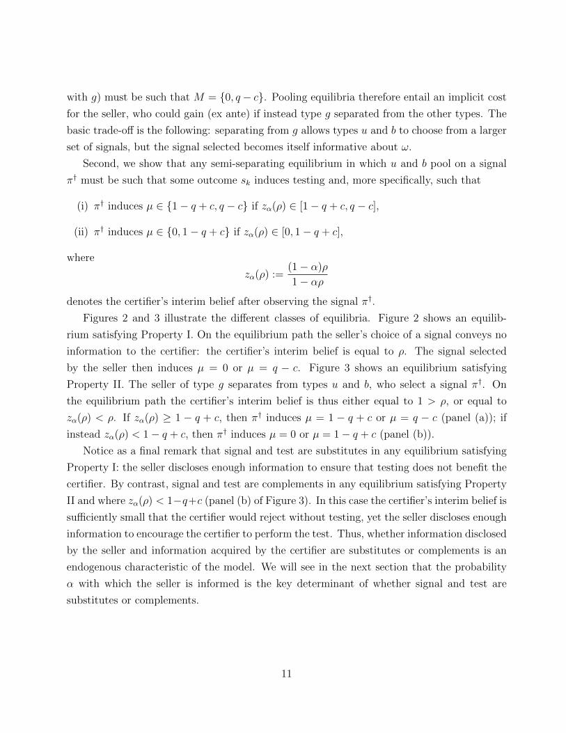
Second, we show that any semi-separating equilibrium in which u and b pool on a signal

π† must be such that some outcome sk induces testing and, more specifically, such that

(i) π† induces µ ∈ {1− q + c, q − c} if zα(ρ) ∈ [1− q + c, q − c],

(ii) π† induces µ ∈ {0, 1− q + c} if zα(ρ) ∈ [0, 1− q + c],

where

zα(ρ) :=(1− α)ρ

1− αρ

denotes the certifier’s interim belief after observing the signal π†.

Figures 2 and 3 illustrate the different classes of equilibria. Figure 2 shows an equilib-

rium satisfying Property I. On the equilibrium path the seller’s choice of a signal conveys no

information to the certifier: the certifier’s interim belief is equal to ρ. The signal selected

by the seller then induces µ = 0 or µ = q − c. Figure 3 shows an equilibrium satisfying

Property II. The seller of type g separates from types u and b, who select a signal π†. On

the equilibrium path the certifier’s interim belief is thus either equal to 1 > ρ, or equal to

zα(ρ) < ρ. If zα(ρ) ≥ 1 − q + c, then π† induces µ = 1 − q + c or µ = q − c (panel (a)); if

instead zα(ρ) < 1− q + c, then π† induces µ = 0 or µ = 1− q + c (panel (b)).

Notice as a final remark that signal and test are substitutes in any equilibrium satisfying

Property I: the seller discloses enough information to ensure that testing does not benefit the

certifier. By contrast, signal and test are complements in any equilibrium satisfying Property

II and where zα(ρ) < 1−q+c (panel (b) of Figure 3). In this case the certifier’s interim belief is

sufficiently small that the certifier would reject without testing, yet the seller discloses enough

information to encourage the certifier to perform the test. Thus, whether information disclosed

by the seller and information acquired by the certifier are substitutes or complements is an

endogenous characteristic of the model. We will see in the next section that the probability

α with which the seller is informed is the key determinant of whether signal and test are

substitutes or complements.

11

zα

ρ

q−c

1−q+c

0

1

(a)

zα

ρ

q−c

1−q+c

0

1

(b)

Figure 3: Equilibrium satisfying Property II

3.2 Two Simple Cases

Say that certification quality (resp. social welfare) is non-decreasing in the technology if in

equilibrium, keeping other parameters fixed, q2 ≥ q1 and c2 ≤ c1 implies Q2 ≥ Q1 (resp.

W2 ≥ W1). Say that certification quality (resp. social welfare) is non-monotonic in the

technology if we can find (q1, c1) and (q2, c2) satisfying q2 > q1, c2 < c1, and such that in

equilibrium Q2 < Q1 (resp. W2 < W1). The next theorem states a bare version of the paper’s

main result.

Theorem 1. In equilibrium, certification quality and social welfare are:

(i) non-decreasing in the technology if α = 1,

(ii) non-monotonic in the technology if α = 0.

To understand part (i) of the theorem note that if α = 1 then the seller is either of type b

or g. By Lemma 2, type b therefore has to pool with g. Hence, by Lemma 3, any equilibrium

satisfies Property I. The remaining step is to note that M = {0, q−c} implies that the approval

probability is equal to 1 conditional on ω = G and equal to ρ(1−q+c)(1−ρ)(q−c) conditional on ω = B.

Hence certification quality increases as a function of q − c (the number of mistakes made by

the certifier goes down as q − c increases). Moreover, as no testing takes place, certification

quality equals social welfare. Thus, social welfare increases as a function of q − c as well.

12

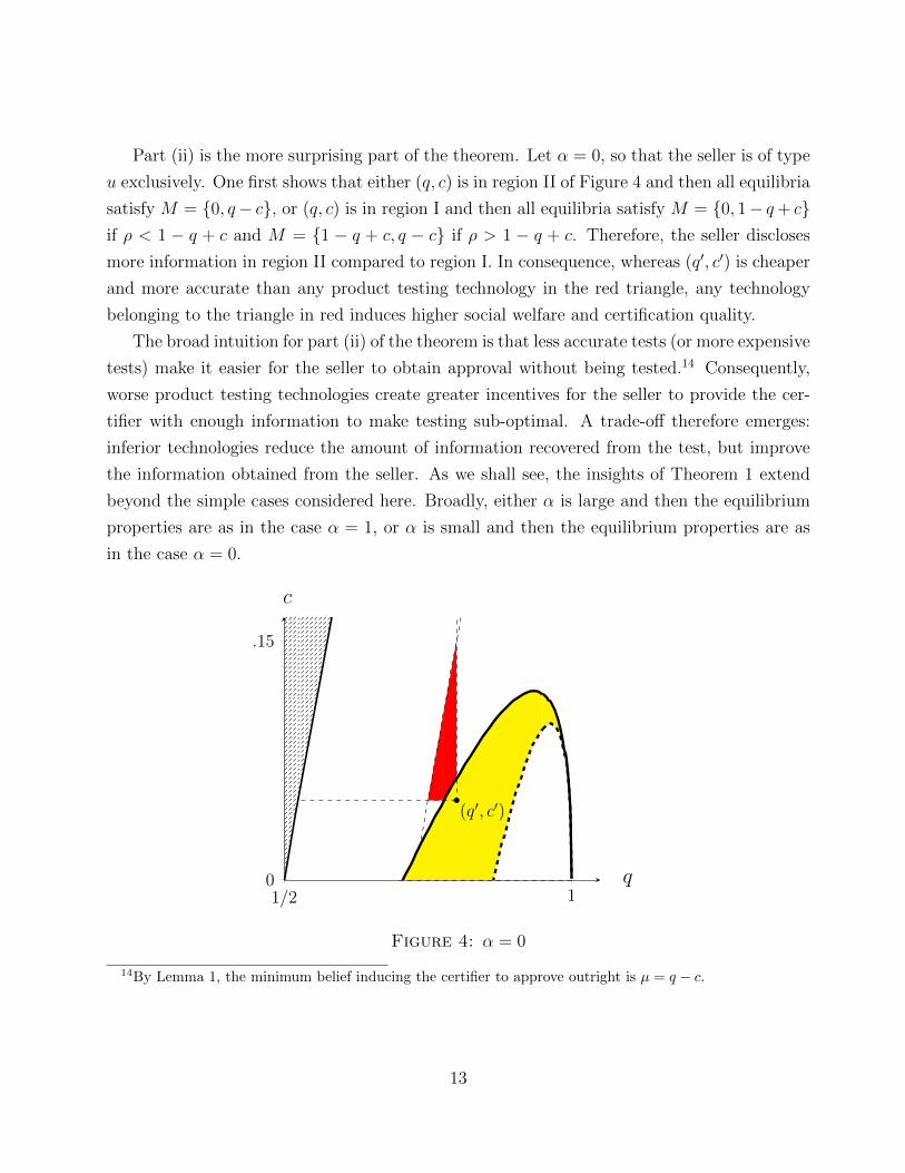
Part (ii) is the more surprising part of the theorem. Let α = 0, so that the seller is of type

u exclusively. One first shows that either (q, c) is in region II of Figure 4 and then all equilibria

satisfy M = {0, q− c}, or (q, c) is in region I and then all equilibria satisfy M = {0, 1− q+ c}if ρ < 1 − q + c and M = {1 − q + c, q − c} if ρ > 1 − q + c. Therefore, the seller discloses

more information in region II compared to region I. In consequence, whereas (q′, c′) is cheaper

and more accurate than any product testing technology in the red triangle, any technology

belonging to the triangle in red induces higher social welfare and certification quality.

The broad intuition for part (ii) of the theorem is that less accurate tests (or more expensive

tests) make it easier for the seller to obtain approval without being tested.14 Consequently,

worse product testing technologies create greater incentives for the seller to provide the cer-

tifier with enough information to make testing sub-optimal. A trade-off therefore emerges:

inferior technologies reduce the amount of information recovered from the test, but improve

the information obtained from the seller. As we shall see, the insights of Theorem 1 extend

beyond the simple cases considered here. Broadly, either α is large and then the equilibrium

properties are as in the case α = 1, or α is small and then the equilibrium properties are as

in the case α = 0.

1/2 10

.15

q

c

(q′, c′)

Figure 4: α = 0

14By Lemma 1, the minimum belief inducing the certifier to approve outright is µ = q − c.

13

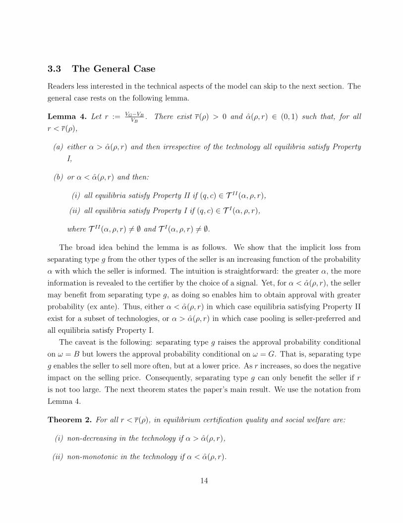
3.3 The General Case

Readers less interested in the technical aspects of the model can skip to the next section. The

general case rests on the following lemma.

Lemma 4. Let r := VG−VBVB

. There exist r(ρ) > 0 and α(ρ, r) ∈ (0, 1) such that, for all

r < r(ρ),

(a) either α > α(ρ, r) and then irrespective of the technology all equilibria satisfy Property

I,

(b) or α < α(ρ, r) and then:

(i) all equilibria satisfy Property II if (q, c) ∈ T II(α, ρ, r),

(ii) all equilibria satisfy Property I if (q, c) ∈ T I(α, ρ, r),

where T II(α, ρ, r) 6= ∅ and T I(α, ρ, r) 6= ∅.

The broad idea behind the lemma is as follows. We show that the implicit loss from

separating type g from the other types of the seller is an increasing function of the probability

α with which the seller is informed. The intuition is straightforward: the greater α, the more

information is revealed to the certifier by the choice of a signal. Yet, for α < α(ρ, r), the seller

may benefit from separating type g, as doing so enables him to obtain approval with greater

probability (ex ante). Thus, either α < α(ρ, r) in which case equilibria satisfying Property II

exist for a subset of technologies, or α > α(ρ, r) in which case pooling is seller-preferred and

all equilibria satisfy Property I.

The caveat is the following: separating type g raises the approval probability conditional

on ω = B but lowers the approval probability conditional on ω = G. That is, separating type

g enables the seller to sell more often, but at a lower price. As r increases, so does the negative

impact on the selling price. Consequently, separating type g can only benefit the seller if r

is not too large. The next theorem states the paper’s main result. We use the notation from

Lemma 4.

Theorem 2. For all r < r(ρ), in equilibrium certification quality and social welfare are:

(i) non-decreasing in the technology if α > α(ρ, r),

(ii) non-monotonic in the technology if α < α(ρ, r).

14

Theorem 2 gives a general version of Theorem 1. For α > α(ρ, r), cheaper and more

accurate technologies help improve social welfare and certification quality. By contrast, for

α < α(ρ, r) a cheaper and more accurate technology may induce lower social welfare and

certification quality. The next proposition records two more equilibrium properties.

Proposition 1. In equilibrium, certification quality is a non-decreasing function of α. More-

over, no testing ever takes place (on the equilibrium path) as long as α > α(ρ, r).

The first part of the proposition follows from noting that either all equilibria satisfy Prop-

erty I and then changing α has no effect, or all equilibria satisfy Property II and then the

information based on which the certifier makes her final decision becomes Blackwell-more-

informative as α increases. The second part of the proposition uses the fact that the product

is never tested in any equilibrium satisfying Property I.

4 Optimal Certification Design

In this section we endogenize the certifier’s product testing technology. We then explore the

ways in which various policies granting commitment power to the certifier can help improve

social welfare and certification quality.

We extend the baseline model of Section 2 by letting the certifier choose the test accuracy

q given an increasing and convex cost function c(q). We assume to start with that this choice

is simultaneous to the certifier’s decision whether or not conduct a test. We refer to this model

as the model without certifier commitment. The baseline model of Section 2 is referred to as

the model with fixed product testing technology. The following proposition characterizes the

set of equilibria.

Proposition 2. An equilibrium without certifier commitment corresponds to an equilibrium

with fixed product testing technology (q, c) = arg max(q,c(q))(q − c(q)).

The logic underlying the proposition is as follows. Suppose that in equilibrium (whether on

path or off path) the certifier ever performs a test using the product testing technology (q, c).

As c > 0 the certifier must base her final decision on the test result. The certifier’s expected

payoff at the time of conducting the test can thus be written as q− c (up to a constant term):

the certifier’s belief that she will be making the correct decision (that is, approve if ω = G and

reject if ω = B) is given by q, and the cost incurred from testing the product is given by c.

15

Hence, if in equilibrium the certifier ever performs a test, she must do so using the technology

maximizing q − c(q).We next examine whether and how granting commitment power to the certifier can help

improve social welfare and certification quality. We first allow the certifier to pre-commit to

a product testing technology at the onset of the game, that is, the certifier is the first mover

and announces a product testing technology (q†, c†), with c† = c(q†). The continuation game

is as in Section 2 with fixed technology (q†, c†). We refer to this model as the model with weak

certifier commitment. The next result is the dual of Theorem 2: as product testing sometimes

crowds out information disclosed by the seller, the certifier could gain by committing to a

relatively inefficient technology.

Proposition 3. Let r < r(ρ). If α < α(ρ, r) then weak certifier commitment can improve

social welfare and certification quality.

Stronger forms of commitment can help improve certification quality and social welfare yet

further. With unlimited commitment power for instance, the certifier could learn ω perfectly

by committing to approve if and only if the signal outcome implies that ω = G with probability

1. However, off the equilibrium path, the latter policy would require the certifier to reject even

though the certifier believes that ω = G with 99% probability. A more realistic alternative

is to consider the possibility for the certifier to pre-commit to a testing strategy at the onset

of the game, that is, the certifier is the first mover and announces a product testing rule as

a function of information disclosed by the seller. We refer to this model as the model with

strong certifier commitment. The following proposition characterizes the equilibrium in this

setting.

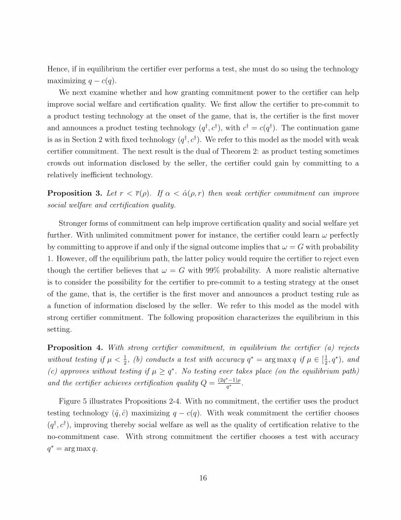
Proposition 4. With strong certifier commitment, in equilibrium the certifier (a) rejects

without testing if µ < 12, (b) conducts a test with accuracy q∗ = arg max q if µ ∈ [1

2, q∗), and

(c) approves without testing if µ ≥ q∗. No testing ever takes place (on the equilibrium path)

and the certifier achieves certification quality Q = (2q∗−1)ρq∗

.

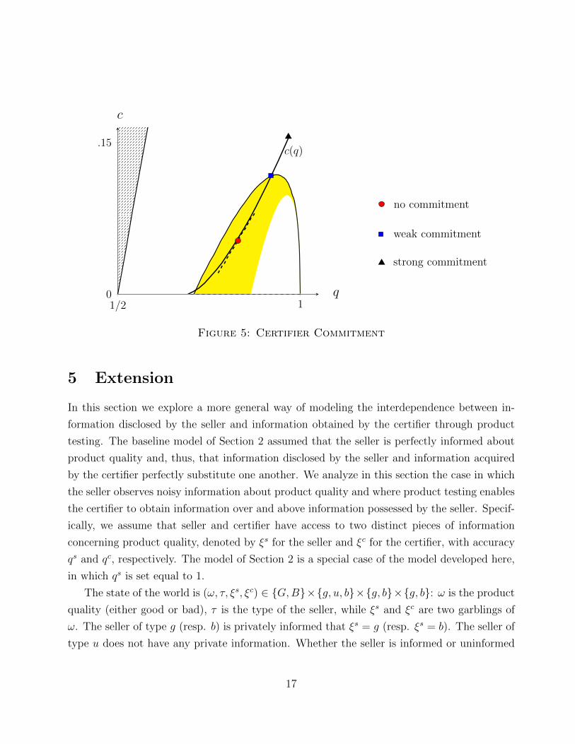
Figure 5 illustrates Propositions 2-4. With no commitment, the certifier uses the product

testing technology (q, c) maximizing q − c(q). With weak commitment the certifier chooses

(q†, c†), improving thereby social welfare as well as the quality of certification relative to the

no-commitment case. With strong commitment the certifier chooses a test with accuracy

q∗ = arg max q.

16

1/2 10

.15

q

c

c(q)

no commitment

weak commitment

strong commitment

Figure 5: Certifier Commitment

5 Extension

In this section we explore a more general way of modeling the interdependence between in-

formation disclosed by the seller and information obtained by the certifier through product

testing. The baseline model of Section 2 assumed that the seller is perfectly informed about

product quality and, thus, that information disclosed by the seller and information acquired

by the certifier perfectly substitute one another. We analyze in this section the case in which

the seller observes noisy information about product quality and where product testing enables

the certifier to obtain information over and above information possessed by the seller. Specif-

ically, we assume that seller and certifier have access to two distinct pieces of information

concerning product quality, denoted by ξs for the seller and ξc for the certifier, with accuracy

qs and qc, respectively. The model of Section 2 is a special case of the model developed here,

in which qs is set equal to 1.

The state of the world is (ω, τ, ξs, ξc) ∈ {G,B}×{g, u, b}×{g, b}×{g, b}: ω is the product

quality (either good or bad), τ is the type of the seller, while ξs and ξc are two garblings of

ω. The seller of type g (resp. b) is privately informed that ξs = g (resp. ξs = b). The seller of

type u does not have any private information. Whether the seller is informed or uninformed

17

is independent of ω, and the probability that he is informed is given by α. To simplify the

exposition we focus in this section on ρ = P(ω = G) = 12

and α ∈ {0, 1}.For i = s, c the joint distribution of (ω, ξi) is given by

g b

G qi 1-qi

B 1-qi qi

where qi ∈ [12, 1]. We assume that ξs and ξc are conditionally independent of one another.

Testing the product allows the certifier to observe ξc, at a cost c > 0. The certifier’s technology

belongs to T = {(qc, c) : qc − c ≥ 12

and qc < 1 − η}. The seller can fully or partly disclose

information by choosing a signal π =(π(·|ξs = g), π(·|ξs = b)

), consisting of a pair of

conditional probability distributions π(·|ξs = g) and π(·|ξs = b) over a set of outcomes S,

with |S| = 2. Conditional on ξs, the outcome of a signal is independent of ω.15 Let Π denote

the set of signals over S. The seller is allowed to choose any signal in Π. Payoffs, timing,

strategies and the equilibrium concept are as in the baseline model of Section 2. We can now

state this section’s main result.

Proposition 5. If(1− qc)qs

(1− qc)qs + qc(1− qs)> qc (1)

holds then, in equilibrium, certification quality and social welfare are:

(i) non-decreasing in the technology if α = 1,

(ii) non-monotonic in the technology if α = 0.

To understand (1), notice that the left-hand side is increasing in qs and tends to 1 as qs

tends to 1.16 Hence, broadly, Proposition 5 says that Theorem 1 continues to hold as long

as the seller’s information is sufficiently precise. The steps leading to Proposition 5 are the

same as those leading to Theorem 1. The main difference is in the equilibrium distribution of

the belief µ: in the context of this section, an equilibrium now satisfies Property II if either

M = {1 − qs, 1 − qc + c, qs} or M = {1 − qc + c, qc − c, qs}, while an equilibrium satisfies

Property I if M = {1 − qs, qc − c}. Intuitively, as the seller possesses noisy information, the

15This must be, given our interpretation, as otherwise the seller would be disclosing information that hedoes not have.

16Notice that (1) is equivalent to P(ω = G|ξs = g, ξc = b) > P(ω = G|ξc = g).

18

seller cannot induce extreme beliefs. In addition, pooling with type g is now less attractive

than in the baseline model. The next result shows that if in the baseline model type g

separated from the other types of the seller then the same must be true in the current setting.

Proposition 6. Assume (1) holds, and fix the product testing technology. If in equilibrium

Property II is satisfied given qs = 1 then Property II is also satisfied given qs < 1.

The intuition behind Proposition 6 is straightforward. We argued in Section 3.1 that signal

and test are substitutes under Property I, but partly complements when Property II holds.

As substituting the test with the signal becomes more complicated the noisier the information

of the seller, the set of technologies for which Property I holds shrinks as qs decreases.

6 Conclusion

This paper explored the interplay between certifiers’ information acquisition about products

and sellers’ voluntary disclosure. We showed that in some circumstances access to cheaper

and more accurate certifier tests can lower social welfare and certification quality, by crowding

out information disclosed by the sellers. Our findings apply among others to markets in which

sellers are able to commit to a disclosure rule before learning the quality of their products.

Our results imply, for instance, that regulators may find it optimal to license certification to

relatively inefficient certification agencies.

19

Appendix A: Notation

We gather in this subsection the notation used in the proofs. A semi-separating equilibrium in

which type g separates from the other types is such that the certifier’s interim belief is either

1 or zα(ρ), where

zα(ρ) :=(1− α)ρ

1− αρ. (2)

Notice that (i) zα(ρ) is strictly decreasing in α, (ii) z0(ρ) = ρ, and (iii) z1(ρ) = 0. We can

thus define α implicitly by zα(ρ) = 1− q + c if ρ > 1− q + c and α = 0 otherwise. With this

notation, either α < α and then zα(ρ) ∈ (1− q+ c, ρ], or α ≥ α and then zα(ρ) ∈ [0, 1− q+ c].

Next, for all x, y such that (1− x)y 6= 0 let

φ(x, y) :=x(1− y)

(1− x)y. (3)

Note that by Bayes’ rule, ifπ(sj |B)

π(sj |G)= φ(x, y) and the certifier’s interim belief induced by π is

equal to x, then µ = y following outcome sj.

Given any signal π let s1 := arg maxsj∈Sπ(sj |B)

π(sj |G)and s2 := arg minsj∈S

π(sj |B)

π(sj |G). With this

notation, the following signals are uniquely determined (up to relabeling of the outcomes).

Define the signal πIIα (q, c, ρ) (or πII for short) as follows:

(i) if α ≥ α then πII(s1|G) = 0 and πII(s2|B)πII(s2|G)

= φ(zα(ρ), 1− q + c),

(ii) if α ≤ α, then πII(s1|B)πII(s1|G)

= φ(zα(ρ), 1− q + c) and πII(s2|B)πII(s2|G)

= φ(zα(ρ), q − c).

Thus, with interim belief zα(ρ), either α ≥ α and then πII induces µ ∈ {0, 1−q+c}, or α ≤ α

and then πII induces µ ∈ {q − c, 1− q + c}. It is straightforward to show that if α ≥ α then{πII(s2|G) = 1 = 1− πII(s1|G),

πII(s2|B) = φ(zα(ρ), 1− q + c) = 1− πII(s1|B),(4)

and if α ≤ α thenπII(s2|G) =

(zα(ρ)− (1− q + c)

)(q − c)(

2(q − c)− 1)zα(ρ)

= 1− πII(s1|G),

πII(s2|B) =

(zα(ρ)− (1− q + c)

)(1− q + c)(

2(q − c)− 1)(1− zα(ρ))

= 1− πII(s1|B).

(5)

20

Next, define the signal πI(q, c, ρ) (or πI for short) as follows: πI(s1|G) = 0 and πI(s2|B)πI(s2|G)

=

φ(ρ, q − c). Thus, with interim belief ρ, πI induces µ ∈ {0, q − c}. Lastly, let π∗ denote the

fully revealing signal, that is, π∗(s1|G) = 0 = π∗(s2|B).

Finally, we will use A to represent the ex ante probability of approval, AG to represent the

probability of approval conditional on ω = G, and AB to represent the probability of approval

conditional on ω = B. Thus,

A = ρAG + (1− ρ)AB. (6)

21

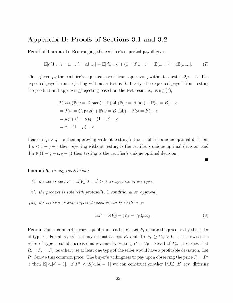
Appendix B: Proofs of Sections 3.1 and 3.2

Proof of Lemma 1: Rearranging the certifier’s expected payoff gives

E[d(1ω=G − 1ω=B)− c1test] = E[d1ω=G + (1− d)1ω=B]− E[1ω=B]− cE[1test]. (7)

Thus, given µ, the certifier’s expected payoff from approving without a test is 2µ − 1. The

expected payoff from rejecting without a test is 0. Lastly, the expected payoff from testing

the product and approving/rejecting based on the test result is, using (7),

P(pass)P(ω = G|pass) + P(fail)P(ω = B|fail)− P(ω = B)− c

= P(ω = G, pass) + P(ω = B, fail)− P(ω = B)− c

= µq + (1− µ)q − (1− µ)− c

= q − (1− µ)− c.

Hence, if µ > q − c then approving without testing is the certifier’s unique optimal decision,

if µ < 1 − q + c then rejecting without testing is the certifier’s unique optimal decision, and

if µ ∈ (1− q + c, q − c) then testing is the certifier’s unique optimal decision.

�

Lemma 5. In any equilibrium:

(i) the seller sets P = E[Vω|d = 1] > 0 irrespective of his type,

(ii) the product is sold with probability 1 conditional on approval,

(iii) the seller’s ex ante expected revenue can be written as

AP = AVB + (VG − VB)ρAG. (8)

Proof: Consider an arbritrary equilibrium, call it E. Let Pτ denote the price set by the seller

of type τ . For all τ , (a) the buyer must accept Pτ and (b) Pτ ≥ VB > 0, as otherwise the

seller of type τ could increase his revenue by setting P = VB instead of Pτ . It ensues that

Pb = Pu = Pg, as otherwise at least one type of the seller would have a profitable deviation. Let

P ∗ denote this common price. The buyer’s willingness to pay upon observing the price P = P ∗

is then E[Vω|d = 1]. If P ∗ < E[Vω|d = 1] we can construct another PBE, E ′ say, differing

22

from E only at the price-setting stage, where all types of the seller set P = E[Vω|d = 1]. The

ex ante expected revenue of the seller is strictly greater in E ′ than it is in E, contradicting

the seller-preferred criterion. This establishes parts (i)-(ii) of the lemma. Finally, by virtue of

parts (i)-(ii), the seller’s ex ante expected revenue can be written as

AE[Vω|d = 1] = A[VBP(ω = B|d = 1) + VGP(ω = G|d = 1)

]= A

[VB + (VG − VB)P(ω = G|d = 1)

]= A

[VB + (VG − VB)

P(ω = G, d = 1)

A

]= AVB + (VG − VB)ρAG.

This shows part (iii) of the lemma.

�

Lemma 6. Consider two PBE, E and E ′. If A′G ≥ AG and A′> A then E does not satisfy

the seller-preferred criterion.

Proof: Suppose that E satisfies the seller-preferred criterion. Applying Lemma 5, the seller’s

ex ante expected revenue in E can then be written as AVB + (VG − VB)ρAG. Next, if in

E ′ the seller ever sets P < E[Vω|d = 1] on the equilibrium path, we can construct another

PBE, call it E ′′, differing from E ′ only at the price-setting stage, and where the seller sets

P = E[Vω|d = 1] irrespective of his type. Therefore, assume without loss of generality that,

in E ′, P = E[Vω|d = 1]. Repeating the arguments in the proof of Lemma 5, the seller’s ex

ante expected revenue in E ′ can then be written as A′VB + (VG − VB)ρA′G. Consequently, if

A′G ≥ AG and A′> A then E ′ is preferred by the seller to E.

�

Lemma 7. For all α > 0, a PBE exists in which all types of the seller select πI .

Proof: Let α > 0 and P † := (q− c)VG + (1− q+ c)VB. We will construct a PBE in which (i)

the seller selects πI (irrespective of his type), (ii) the seller sets P = P †, and (iii) the buyer

accepts the price P †. Given (i), applying Bayes’ rule, the certifier’s interim belief induced by

πI is equal to ρ. Hence, by virtue of Lemma 1, selecting πI induces probability πI(s2|G) = 1

of obtaining approval conditional on ω = G, and probability πI(s2|B) = ρ(1−q+c)(1−ρ)(q−c) of obtaining

23

approval conditional on ω = B. Thus, (i) implies that

E[Vω|d = 1] = P(ω = G|d = 1)VG + P(ω = B|d = 1)VB

=1

P(d = 1)

[ρVG + (1− ρ)

ρ(1− q + c)

(1− ρ)(q − c)VB

]= (q − c)VG + (1− q + c)VB

= P †.

Hence, the price P † is acceptable to the buyer whenever (i) and (ii) hold. Next, set the

certifier’s interim belief equal to 0 for all signals other than πI , and set the buyer’s belief

equal to 0 for all prices other than P †. Then to show that (i)-(ii) form part of a PBE it is

sufficient to show that no type of the seller is able to obtain approval with strictly greater

probability by selecting a signal different from πI . This is clear for the seller of type g, since by

selecting πI type g is approved with probability 1, and also for the seller of type b, since any

signal different from πI gives probability 0 of approval for type b. Now consider type u. Note

first that any signal different from πI and π∗ is such that type u obtains approval with strictly

smaller probability than he would obtain by selecting π∗. Moreover, π∗ gives probability ρ

of approval to the seller of type u, whereas πI gives probability of approval ρq−c > ρ. This

establishes that (i)-(iii) form part of a PBE.

�

Lemma 8. For all α > 0, any PBE such that either M = {0, q − c, 1} or M = {0, 1} fails to

satisfy the seller-preferred criterion.

Proof: Suppose a PBE exists, call it E, such that either M = {0, q − c, 1} or M = {0, 1}.Let E ′ denote a PBE in which all types of the seller select πI (such a PBE exists, by Lemma

7). By Lemma 1, we have A′G ≥ AG, A′B > AB and, by (6), A′> A. Hence, by Lemma 6, E

violates the seller-preferred criterion.

�

Proof of Lemma 2: For α > 0 part (i) of the lemma follows from Lemma 8. For α = 0 just

note that the probability of approval is strictly greater if the seller selects a signal inducing

M = {0, q − c} than if the seller selects a signal inducing M = {0, 1}. Part (ii) follows from

noting that type g can guarantee himself approval with probability 1 by selecting π∗.

We now prove part (iii) of the lemma. Let α > 0 and suppose that a seller-preferred PBE

exists in which the seller of type b separates from the other two types of the seller, and call it

24

PBE E. Let π1 denote the signal selected by the seller of type u, and π2 the signal selected

by the seller of type g. Both π1 and π2 must induce probability 0 of approval conditional on

ω = B, as otherwise type b would have a profitable deviation; call this Condition C. We will

show that we obtain a contradiction, whether π1 = π2 or π1 6= π2.

Case 1: π1 = π2. As type g must be approved with probability 1, combining Condition C and

Lemma 1 gives M = {0, 1}, contradicting part (i) of the lemma.

Case 2: π1 6= π2. Combining Condition C and Lemma 1 shows that, for all sj ∈ S such

that π1(sj|G) > 0, either π1(sj|B) = 0 orπ1(sj |B)

π1(sj |G)> φ(ρ, 1 − q + c). Suppose, for the sake of

argument, that we can find sk ∈ S such that π1(sk|G) > 0 and π1(sk|B)π1(sk|G)

> φ(ρ, 1−q+c). Let E ′

denote a PBE in which, irrespective of his type, the seller selects π∗ and sets P = VB (clearly,

such a PBE exists). We then have A′G ≥ AG + (1 − α)π1(sk|G) and A′B = AB = 0. Thus,

A′G > AG, A′B = AB and, by (6), A′> A. It now follows by Lemma 6 that E must violate

the seller-preferred criterion, contradicting the definition of E. Therefore, for all sj ∈ S,

π1(sj|G) > 0 implies π1(sj|B) = 0, that is π1 = π∗. Reasoning as in Case 1 now leads to

another contradiction.

Lastly, to see that the last part of the lemma must hold, notice that if a pooling equilibrium

existed in which the product were to be tested then, as q < 1, type g would be rejected with

positive probability, contradicting part (ii) of the lemma.

�

Lemma 9. Let α > 0. Any equilibrium is either pooling, or semi-separating with type b

pooling with exactly one other type of the seller.

Proof: The lemma is a corollary of part (iii) of Lemma 2.

�

Lemma 10. Let α > 0. Any equilibrium either satisfies Property I or is semi-separating with

type g separating from u and b.

Proof: By Lemma 9, we only need to show that any pooling equilibrium and any semi-

separating equilibrium where type b pools with g must satisfy Property I. We start with

pooling equilibria. Let ΠI(q, c, ρ) ⊂ Π denote the set of signals π such that, for all outcome

sj ∈ S, either π(sj|G) = 0 orπ(sj |B)

π(sj |G)≤ φ(ρ, q − c) (thus πI ∈ ΠI(q, c, ρ)). Suppose that an

25

equilibrium exists, call it E, in which all types of the seller pool on a signal π†. In E, the

certifier’s interim belief induced by π† equals ρ. Hence, by Lemma 1, π† ∈ ΠI , as otherwise

the seller of type g could profitably deviate by selecting π∗. Suppose that π† 6= πI . Applying

Lemma 7 we can find a PBE, call it E ′, in which all types of the seller pool on πI . We then

have A′G = 1 = AG and A′B > AB, and, by (6), A′> A. Hence, by Lemma 6, E violates

the seller-preferred criterion, contradicting the definition of E. Therefore, π† = πI . We thus

obtain M = {0, q − c}.Next, suppose that an equilibrium exists in which the sellers of type g and b pool on a

signal π1 while type u selects a signal π2 6= π1. Applying Bayes’ rule, the certifier’s interim

belief is ρ following the signal π1 and also ρ following the signal π2. Since type g must be

approved with probability 1, Lemma 1 gives π1 ∈ ΠI(q, c, ρ). Next, as selecting π2 is not a

profitable deviation for type b, the probability of obtaining approval conditional on ω = B is

at least as large with π1 as it is with π2. Similarly, as selecting π2 is not a profitable deviation

for type g, the probability of obtaining approval conditional on ω = G is at least as large

with π1 as it is with π2. Yet selecting π1 is not a profitable deviation for type u. Hence,

the probability of approval conditional on ω = B must be with π1 the same as it is with π2,

and the probability of approval conditional on ω = G must be with π1 the same as it is with

π2. Since we found above that π1 ∈ ΠI(q, c, ρ), Lemma 1 now gives π2 ∈ ΠI(q, c, ρ). Lastly,

reasoning as in the first part of the proof yields π1 = π2 = πI . We thus obtain M = {0, q− c}.�

Lemma 11. Let α > 0. In any semi-separating equilibrium with type g separating from the

other types of the seller, types u and b select the signal πII .

Proof: We show the proof for the case zα(ρ) ∈ [1 − q + c, q − c]. The proof for the case

zα(ρ) ∈ [0, 1 − q + c] is similar and therefore omitted. Suppose that we can find a semi-

separating equilibrium, call it E, with type g separating from the other types of the seller.

Let π† denote the signal selected by u and b. We will prove that π† = πII .

Step 1: for all sj ∈ S, π†(sj|G) > 0 impliesπ†(sj |B)

π†(sj |G)≥ φ(zα(ρ), q − c). Suppose for a contra-

diction that we can find sk ∈ S such that π†(sk|G) > 0 and π†(sk|B)π†(sk|G)

< φ(zα(ρ), q− c). We will

construct a PBE E ′ in which A′> A and A′G ≥ AG. Let type g select π∗ while u and b pool

26

on the signal π′ defined by {π′(·|G) = π†(·|G),

π′(sk|B) = π′(sk|G)φ(zα(ρ), q − c).

Thus, in particular, π′(sk|B) > π†(sk|B). Next, let the seller choose P = VB. Lastly, set the

certifier’s interim belief equal to 0 for any signal different than π′ and π∗, and set the buyer’s

belief equal to 0 for any price other than VB. Applying Lemma 1 gives

A′B − AB ≥(π′(sk|B)− π†(sj|B)

)(1− (1− q)),

and

A′G − AG ≥ 0.

Hence, A′G ≥ AG and A′B > AB. As neither type u nor type b had a profitable deviation in E,

neither of the two types can have a profitable deviation in E ′. Thus E ′ is a PBE. Moreover,

A′G ≥ AG and, by (6), A′> A, contradicting Lemma 6.

Step 2: π†(s1|G) = 0 implies π†(s2|B)π†(s2|G)

= φ(zα(ρ), q − c). By Step 1, we only need to show that

π†(s1|G) = 0 implies π†(s2|B)π†(s2|G)

≤ φ(zα(ρ), q − c). Suppose for a contradiction that π†(s1|G) = 0

and π†(s2|B)π†(s2|G)

> φ(zα(ρ), q − c). We will construct a PBE E ′ in which A′> A and A′G ≥ AG.

Let type g select π∗ while u and b pool on the signal πII . Next, let the seller choose P = VB.

Lastly, set the certifier’s interim belief equal to 0 for any signal different than πII and π∗, and

set the buyer’s belief equal to 0 for any price other than VB. Applying Lemma 1 gives

A′B − AB ≥ πII(s2|B)(1− (1− q)

),

and

A′G − AG ≥ 0.

Hence, A′G ≥ AG and A′B > AB. As neither type u nor type b had a profitable deviation in E,

neither of the two types can have a profitable deviation in E ′. Thus E ′ is a PBE. Moreover,

A′G ≥ AG and, by (6), A′> A, contradicting Lemma 6.

Step 3: for all sj ∈ S, π†(sj|G) > 0. Suppose that π†(s1|G) = 0. By Step 2, π†(s2|B)π†(s2|G)

=

φ(zα(ρ), q−c). Thus M = {0, q−c, 1} which, by virtue of Lemma 8, contradicts the definition

27

of E.

Step 4:π†(sj |B)

π†(sj |G)≤ φ(zα(ρ), 1− q + c), for all sj ∈ S. Suppose for a contradiction that we can

find sk ∈ S such that π†(sk|B)π†(sk|G)

> φ(zα(ρ), 1 − q + c). We will construct a PBE E ′ in which

A′> A and A′G ≥ AG. Let type g select π∗ while u and b pool on the signal π′ defined by{

π′(·|B) = π†(·|B),

π′(sk|G) = 0.

Thus, in particular, π′(sk|G) < π†(sk|G) while π′(s−k|G) > π†(s−k|G). Next, let the seller

choose P = VB. Lastly, set the certifier’s interim belief equal to 0 for any signal different than

π′ and π∗, and set the buyer’s belief equal to 0 for any price other than VB. As zα(ρ) ≥ 1−q+c,

applying Lemma 1 gives

A′B − AB ≥ 0,

and

A′G − AG ≥ q(1− α)(π′(s−k|G)− π†(s−k|G)

).

Hence, A′G > AG and A′B ≥ AB. As neither type u nor type b had a profitable deviation in E,

neither of the two types can have a profitable deviation in E ′. Thus E ′ is a PBE. Moreover,

A′G ≥ AG and, by (6), A′> A, contradicting Lemma 6.

Step 5: π†(s1|B)π†(s1|G)

= φ(zα(ρ), 1 − q + c) and π†(s2|B)π†(s2|G)

= φ(zα(ρ), q − c). By Steps 1 and 4,π†(sj |B)

π†(sj |G)∈ [φ(zα(ρ), q − c), φ(zα(ρ), 1− q + c)] for all sj ∈ S. Suppose for a contradiction that

π†(s1|B)π†(s1|G)

< φ(zα(ρ), 1 − q + c) and π†(s2|B)π†(s2|G)

= φ(zα(ρ), q − c). We will construct a PBE E ′ in

which A′> A and A′G ≥ AG. Let type g select a signal in Π∗ while u and b pool on the signal

π′ defined by {π′(·|B) = π†(·|B),

π′(s1|B) = π′(s1|G)φ(zα(ρ), 1− q + c).

Thus, in particular, π′(s1|G) < π†(s1|G) while π′(s2|G) > π†(s2|G). Next, let the seller choose

P = VB. Lastly, set the certifier’s interim belief equal to 0 for any signal different than π′ and

28

π∗, and set the buyer’s belief equal to 0 for any price other than VB. Applying Lemma 1 gives

A′B = AB,

and

A′G − AG = (1− α)(1− q)(π′(s2|G)− π†(s2|G)

).

Hence, A′G > AG and A′B = AB. As neither type u nor type b had a profitable deviation

in E, neither of the two types can have a profitable deviation in E ′. Thus E ′ is a PBE.

Moreover, A′G ≥ AG and, by (6), A′> A, contradicting Lemma 6. One shows that assuming

π†(s1|B)π†(s1|G)

= φ(zα(ρ), 1 − q + c) and π†(s2|B)π†(s2|G)

> φ(zα(ρ), q − c) leads to a similar contradiction.

Finally, assumingπ†(sj |B)

π†(sj |G)∈ (φ(zα(ρ), q− c), φ(zα(ρ), 1− q+ c)) for all sj ∈ S leads to a similar

contradiction as well.

Step 5 shows that π† = πII and concludes the proof of the lemma.

�

Proof of Lemma 3: Combining Lemmata 10 and 11 shows that the statement of Lemma

3 holds for α > 0. We next consider the special case α = 0. Let f(µ) denote the seller’s

expected revenue given µ. Applying Lemmata 1 and 5,

f(µ) =

0 for µ ∈ [0, 1− q + c)(µq + (1− µ)(1− q)

)P for µ ∈ [1− q + c, q − c)

P for µ ∈ [q − c, 1],

(9)

where P = E[Vω|d = 1]. Let cavf denote the concavification of the function f . By (9),

cavf(x) > f(x) if x ∈ (0, 1 − q + c) ∪ (1 − q + c, q − c), and cavf(x) = f(x) if x ∈ [q − c, 1].

Since ρ ≤ 12< q − c, standard concavification arguments yield M ⊆ {0, 1− q + c, q − c} (see,

e.g. Kamenica and Gentzkow (2011)). Moreover, either

(q − c)− (1− q + c)

q − cf(0) +

(1− q + c

q − c

)f(q − c) > f(1− q + c), (10)

in which case M = {0, q− c}, or the inequality in (10) is reversed and then M = {0, 1− q+ c}if ρ < 1− q + c and M = {1− q + c, q − c} if ρ > 1− q + c.

�

29

Lemma 12. Both T I(0, ρ) and T II(0, ρ) are non-empty sets. Moreover,

T II(0, ρ) =

{(q, c) :

1√2< q < 1 and 0 < c <

4q2 − 3q − 1 +√q2 − 6q + 5

2(2q − 1)

}.

Proof: We saw in the proof of Lemma 3 that in equilibrium either (10) holds and then

M = {0, q−c}, or the inequality in (10) is reversed and then M = {0, 1−q+c} if ρ < 1−q+c

and M = {1− q+ c, q− c} if ρ > 1− q+ c. Thus (q, c) ∈ T II(0, ρ) if and only if the inequality

in (10) is reversed, that is, if and only if

(1− q + c)q + (q − c)(1− q) > 1− q + c

q − c.

This inequality is equivalent to

(2q − 1)c2 + (1 + 3q − 4q2)c− (1− q)(2q2 − 1) < 0,

which in turn is equivalent to q ∈ ( 1√2, 1) and c <

4q2−3q−1+√q2−6q+5

2(2q−1) . Hence both T II(0, ρ)

and T I(0, ρ) are non-empty sets.

�

Proof of Theorem 1: Case α = 1: In any equilibrium, by Lemma 2, type b pools with g and

g is approved with probability 1. Hence, combining Lemmata 1 and 7 gives M = {0, q − c}.Thus (i) the product is never tested on the equilibrium path, and (ii) the information based

on which the certifier makes her final decision becomes Blackwell-more-informative as q − cincreases.

Case α = 0: By Lemma 12, both T I(0, ρ) and T II(0, ρ) are non-empty sets. Let F(0, ρ)

denote the frontier between these two sets. Thus (q, c) ∈ F(0, ρ) implies that the seller is

indifferent between selecting the signal πII and selecting the signal πI , that is, both signals

lead to the same probability of approval. On the other hand, P(d = 1|ω = G) = 1 if the seller

selects πI whereas, using (5),

P(d = 1|ω = G) ≤ 1− (1− q) minα≤α

πIIα (s1|G) = 1− (1− q)(1− q + c)

if the seller selects πII . Thus, certification quality jumps down as one crosses over from T I(0, ρ)

to T II(0, ρ). Moreover, since the product is never tested in T I(0, ρ) but is sometimes tested

30

in T II(0, ρ), social welfare also jumps down as one crosses over from T I(0, ρ) to T II(0, ρ).

�

31

Appendix C: Proofs of Section 3.3

Lemma 13. The seller’s ex ante expected revenue is(

ρq−c

)VB +(VG−VB)ρ in any equilibrium

satisfying Property I,[αρ+(1− αρ)

(zα(ρ)− (1− q + c)

2(q − c)− 1+

(q − c)− zα(ρ)

2(q − c)− 1

((1− q + c)q + (q − c)(1− q)

))]VB

+ (VG − VB)ρ[1− (1− α)πII(s1|G)(1− q)

]in any equilibrium satisfying Property II if α ≤ α (with πII(s1|G) given by (5)), and

[αρ+ (1− αρ)

((1− q + c)q + (q − c)(1− q)

) zα(ρ)

1− q + c

]VB + (VG − VB)ρ[α + (1− α)q]

in any equilibrium satisfying Property II if α ≥ α.

Proof: The lemma applies (8) using Lemma 1.

�

Lemma 14. There exists α† > 0 and r† > 0 such that if α < α† and r < r† then T I(α, ρ, r)and T II(α, ρ, r) are both non-empty sets.

Proof: Immediate from (8), Lemma 12 and continuity of the seller’s expected revenues in

Lemma 13.

�

Lemma 15. Both πII(s2|G) and πII(s2|B) are strictly decreasing functions of α for α ∈ [0, α].

Similarly, πII(s2|B) (resp. πII(s2|G) ) is a strictly (resp. weakly) decreasing function of α for

α ∈ [α, 1].

Proof: The first part follows from (5) and the second part follows from (4).

�

Lemma 16. If given α1 > 0 a PBE exists which satisfies Property II then a PBE satisfying

Property II exists for all α2 < α1.

Proof: Assume that, given α1 > 0, a PBE exists within the class of PBE satisfying Property

II, and let Yα1 denote type u’s probability of approval in this PBE. Then Yα1 ≥ ρ, as otherwise

32

type u could profitably deviate by selecting π∗. Now consider α2 < α1. We will show that a

PBE exists such that (i) type g selects π∗, (ii) types b and u select πIIα2(q, c, ρ), (iii) the seller

sets P = VB irrespective of his type, (iv) the certifier’s interim belief equals 0 for any signal

different than πII and π∗, and (v) the buyer’s belief equals 0 for any price other than VB.

Given (i)-(v), neither type b nor type g have an incentive to deviate. So we only need to show

that type u does not have a profitable deviation. Moreover, the only candidate profitable

deviation is to select π∗. Let Yα2 denote type u’s probability of approval from selecting πII

whenever (i)-(v) hold. As π∗ induces approval with probability ρ for the seller of type u, we

only need to show that Yα2 ≥ ρ, and since we argued above that Yα1 ≥ ρ, it is sufficient to

show that Yα2 ≥ Yα1 . Below, we consider the different cases.

Case 1: α ≤ α2 < α1. We have in this case

Yα2 − Yα1 = (1− ρ)(1− q)(πIIα2

(s2|B)− πIIα1(s2|B)

).

Therefore, Yα2 − Yα1 ≥ 0, by virtue of Lemma 15.

Case 2: α2 < α < α1. We have in this case

Yα2 − Yα1 ≥ (1− ρ)(1− q)πIIα1(s1|B).

Therefore, Yα2 − Yα1 ≥ 0.

Case 3: α2 < α1 ≤ α. We have in this case

Yα2 − Yα1 =(1− ρ)(1− (1− q))(πIIα2

(s2|B)− πIIα1(s2|B)

)+ ρ(1− q)

(πIIα2

(s2|G)− πIIα1(s2|G)

).

Therefore, Yα2 − Yα1 ≥ 0, by virtue of Lemma 15.

�

Lemma 17. Let Eα denote a PBE satisfying Property II, Aα the ex ante probability of approval

in Eα, and Pα := E[Vω|d = 1] evaluated in Eα. There exists M(ρ) > 0 such that dAαdα

< −M(ρ),

and m(ρ) > 0 such that dPαdα

< m(ρ)(VG − VB).

Proof: By Lemma 16, if given α1 a PBE exists within the class of PBE satisfying Property

33

II then the same is true for all α < α1. Thus the existence of a PBE Eα satisfying Property

II implies (q, c) ∈ T II(0, ρ) ∪ F(0, ρ). By Lemma 12, we can therefore pick η > 0 such that

q − c > 12

+ η. Now, either α ≥ α and then

Aα = ρ[α + (1− α)q] + (1− ρ)(1− q)πIIα (s2|B), (11)

or α < α and then

Aα = ρ[α + (1− α)

(πIIα (s2|G) + qπIIα (s1|G)

)]+ (1− ρ)

(πIIα (s2|B) + (1− q)πIIα (s1|B)

).

(12)

Substituting (4) into (11) and simplifying the expression on the right-hand side gives, for

α ≥ α,

Aα = K − αρ(1− q)(

2(q − c)− 1

1− q + c

), (13)

with K independent of α. Similarly, substituting (5) into (12) and simplifying the expression

on the right-hand side gives, for α < α,

Aα = K ′ − αρ(1− q + c)

2(q − c)− 1

[q(q − c)− (1− q)(1− q + c)

], (14)

with K ′ independent of α. Hence, given (13), (14), q − c > 12

+ η and q < 1− η, we obtain

dAαdα

< −ρηη,

which shows the first part of the lemma.

We now show the second part of the lemma. Observe first that we can write

Pα = VB + (VG − VB)P(ω = G|d = 1).

Moreover, either α ≥ α and then

P(ω = G|d = 1) =ρ(α + (1− α)q)

ρ(α + (1− α)q) + (1− ρ)(1− q)πIIα (s2|B),

34

or α < α and then

P(ω = G|d = 1) =ρ[α + (1− α)

(πIIα (s2|G) + qπIIα (s1|G)

)]ρ[α + (1− α)

(πIIα (s2|G) + qπIIα (s1|G)

)]+ (1− ρ)

(πIIα (s2|B) + (1− q)πIIα (s1|B)

) .Straightforward algebra now yields

dPαdα

< (VG − VB)(

2 +1

η

)2

ρ

for α ≥ α, and

dPαdα

< (VG − VB)(

1 +1

η

)4

ρ

for α < α.

�

Lemma 18. Let Eα denote a PBE satisfying Property II and such that the seller sets P =

E[Vω|d = 1]. There exists r(ρ) > 0 such that, if r < r(ρ), then the seller’s ex ante expected

revenue in Eα is a strictly decreasing function of α.

Proof: Let Pα := E[Vω|d = 1] evaluated in Eα. The seller’s ex ante expected revenue in Eα

is therefore AαPα. Applying Lemma 17,

d

dα

(AαPα

)< −M(ρ)Pα +m(ρ)(VG − VB)Aα.

As Pα ≥ VB and Aα ≤ 1, we obtain ddα

(AαPα

)< −M(ρ)VB + m(ρ)(VG − VB). Choosing

r(ρ) = M(ρ)m(ρ)

then gives ddα

(AαPα

)< 0 whenever VG−VB

VB< r(ρ).

�

Lemma 19. There exists r(ρ) > 0 such that, if r < r(ρ), then T II(α1, ρ, r) ⊆ T II(α2, ρ, r)

for all α1 ≥ α2.

Proof: The result is trivial if T II(α1, ρ, r) = ∅. So assume that T II(α1, ρ, r) 6= ∅ and let

(q, c) ∈ T II(α1, ρ, r). Let α2 ≤ α1. We will show that (q, c) ∈ T II(α2, ρ, r). Let Eα1 denote

an equilibrium given α = α1, and let Aα1Pα1 denote the seller’s ex ante expected revenue in

this PBE. By Lemma 16, with α = α2 a PBE exists which satisfies Property II. Moreover,

35

we can choose this PBE to be such that the seller sets P = E[Vω|d = 1]. Call this PBE Eα2 .

Now, applying Lemma 18 gives Aα2Pα2 > Aα1Pα1 and, since Eα1 is a seller-preferred PBE,

combining Lemmata 7 and 13 gives Aα1Pα1 ≥(

ρq−c

)VB + (VG − VB)ρ. Thus

Aα2Pα2 >( ρ

q − c

)VB + (VG − VB)ρ,

which by Lemma 13 implies that (q, c) ∈ T II(α2, ρ, r). As (q, c) was chosen arbitrarily, we

obtain T II(α1, ρ, r) ⊆ T II(α2, ρ, r).

�

Proof of Lemma 4: Lemma 4 is obtained from the combination of Lemmata 14 and 19. The

fact that α(ρ, r) < 1 follows from the observation made in the proof of part (i) of Theorem 1

that T II(1, ρ, r) = ∅.�

Lemma 20. In equilibrium, certification quality is a continuous function of (q, c) for all

(q, c) ∈ T I(α, ρ, r) ∪ T II(α, ρ, r).

Proof: We have

Q = E[d(1ω=G − 1ω=B)]

= E[d1ω=G + (1− d)1ω=B − 1ω=B] (15)

= E[d1ω=G + (1− d)1ω=B]− (1− ρ).

Certification quality thus equals the probability that the certifier makes a correct decision

(that is, approve when ω = G and reject when ω = B) minus the probability that ω = B.

Using (15) and Lemma 1, if (q, c) ∈ T I(α, ρ, r) then, in equilibrium,

Q = 1− ρ(1− q + c)

(q − c)− (1− ρ). (16)

Similarly, if (q, c) ∈ T II(α, ρ, r), then either α < α, in which case

Q =αρ+ (1− αρ)

[zα(ρ)− (1− q + c)

2(q − c)− 1

(q − c

)+

(q − c)− zα(ρ)

2(q − c)− 1q

]− (1− ρ),

36

or α ≥ α, in which case

Q =αρ+ (1− αρ)

[(1− q + c)− zα(ρ)

1− q + c+

zα(ρ)

1− q + cq

]− (1− ρ).

�

Proof of Theorem 2:

Proof of (i): For α > α(ρ, r), all equilibria satisfy Property I. Hence, by Lemma 1, the

product is never tested on the equilibrium path and social welfare equals certification quality.

Moreover, in this case, certification quality is given by (16), and is therefore increasing in

q − c. This establishes part (i) of the theorem.

Proof of (ii): Let α ∈(0, α(ρ, r)

)(the case α = 0 was treated in Theorem 1), and pick

a technology (qF , cF) on the frontier F(α, ρ, r) between T II(α, ρ, r) and T I(α, ρ, r). Since

Lemma 12 established that

F(0, ρ) =

{(q, c) :

1√2< q < 1 and c =

4q2 − 3q − 1 +√q2 − 6q + 5

2(2q − 1)

},

we can (in view of Lemma 19) choose sequences {(qn, cn)}n≥1 and {(q†n, c†n)}n≥1 tending to

(qF , cF) as n tends to infinity, with (qn, cn) ∈ T II(α, ρ, r), (q†n, c†n) ∈ T I(α, ρ, r), cn < c†n, and

qn > q†n. We will show that, for n large enough, in equilibrium certification quality is strictly

higher with technology (q†n, c†n) than with technology (qn, cn).

Let En denote an equilibrium with technology (qn, cn) and E†n denote an equilibrium with

technology (q†n, c†n). Let An (resp. A

†n) denote the ex ante probability of approval in equilibrium

En (resp. E†n) and Pn (resp. P †n) denote the price of the seller in this equilibrium. The

combination of Lemmata 7 and 20 yields

limn→∞

A†nP†n ≤ lim

n→∞AnPn.

Hence,

limn→∞An

limn→∞A†n

≥ limn→∞ P†n

limn→∞ Pn≥ VBVG

=1

1 + r,

37

from which

limn→∞

An > limn→∞

A†n − r. (17)

Next, let AGn (resp. A†Gn) denote the probability of approval conditional on ω = G in equi-

librium En (resp. E†n). By Lemma 1, A†Gn = 1, whereas

AGn ≤ 1− (1− α)(1− q) minα≤α

πIIα (s1|G) = 1− (1− α)(1− q)(1−max

α≤απIIα (s2|G)

).

Now, by (5),

maxα≤α

πIIα (s2|G) ≤(12− (1− q + c)

)(q − c)(

2(q − c)− 1)12

= q − c.

Thus,

AGn ≤ 1− (1− α)(1− q)(1− q + c)

and, as α < α and 1− q > η, AGn ≤ 1− (1− α)η2. We thus obtain A†Gn − AGn ≥ (1− α)η2,

and as this holds for all n,

limn→∞

A†Gn − limn→∞

AGn ≥ (1− α)η2. (18)

Since An = ρAGn + (1− ρ)ABn and A†n = ρA†Gn + (1− ρ)A†Bn, we can write

limn→∞

An − limn→∞

A†n = ρ( lim

n→∞AGn − lim

n→∞A†Gn) + (1− ρ)( lim

n→∞ABn − lim

n→∞A†Bn). (19)

Combining (17)-(19) yields

limn→∞

ABn − limn→∞

A†Bn >ρ(1− α)η2 − r

1− ρ. (20)

Lastly, applying (15),

Q†n −Qn = ρ(A†Gn − AGn) + (1− ρ)(ABn − A†Bn),

and thus, using (18) and (20),

limn→∞

Q†n − limn→∞

Qn > 2ρ(1− α)η2 − r.

Choosing N large enough and r sufficiently small gives Q†N > QN . As qN > q†N and cN < c†N ,

38

we have established that certification quality is non-monotonic in the technology. We then

obtain

W †N = Q†N − Γ†N = Q†N > QN > Qn − ΓN = WN .

Consequently, social welfare is non-monotonic in the technology.

�

Proof of Proposition 1: By Lemma 4, either (q, c) ∈ T I(α, ρ, r) for all α or we can find

α(ρ, r) such that (q, c) ∈ T I(α, ρ, r) for all α > α(ρ, r), and (q, c) ∈ T II(α, ρ, r) for all

α < α(ρ, r). In the first case, certification quality is constant for all α ∈ [0, 1]. In the second

case, certification quality is a constant function of α as long as α > α(ρ, r). For α < α(ρ, r),

the information based on which the certifier makes her final decision becomes Blackwell-more-

informative as α increases. Thus certification quality is strictly increasing in α for α < α(ρ, r).

Lastly, we established in the proof of Theorem 2 that certification quality exhibits an upward

jump as one crosses F(α, ρ, r) from within T II(α, ρ, r). Hence, certification quality is greater

for all α > α(ρ, r) than for any α < α(ρ, r). This shows that certification quality is a non-

decreasing function of α in the second case too.

�

39

Appendix D: Proofs of Section 4

Proof of Proposition 2: Suppose that in equilibrium (whether on path or off path) the

certifier ever performs a test using the product testing technology (q, c). As c > 0 the certifier

must base her final decision on the test result. Using (7), the certifier’s expected payoff at the

time of conducting the test can thus be written as q − c − (1 − µ). Hence, if in equilibrium

the certifier ever performs a test, she must do so using the technology maximizing q − c(q).�

Proof of Proposition 3: Combining Theorem 1 and Proposition 2 yields Proposition 3.

�

Lemma 21. With strong certifier commitment the certifier’s equilibrium expected payoff is

bounded above by (2q∗−1)ρq∗

, where q∗ = arg max q.

Proof: Let β denote the certifier’s belief that ω = G at the time of making her final decision.

In any equilibrium, the certifier approves if β > 12

and rejects if β < 12. As µ > q∗ implies

β > 12, in any equilibrium the seller is guaranteed approval anytime µ > q∗. Define the signal

π† such that π†(s1|G) = 0 and π†(s2|B) = φ(ρ, q∗). By pooling on π† the seller thus obtains

approval with probability 1 conditional on ω = G and probability φ(ρ, q∗) conditional on

ω = B. Lemma 6 now shows that A ≥ ρ+ (1− ρ)φ(ρ, q∗) = ρq∗

in any equilibrium. Hence, in

any equilibrium, Q is bounded above by ρ+ (1− ρ)(

1− ρ1−ρ

(1q∗− 1))

= (2q∗−1)ρq∗

.

�

Proof of Proposition 4: By Lemma 21 we only need to show that by choosing the testing

strategy in the statement of the proposition the certifier obtains expected payoff (2q∗−1)ρq∗

.

Reasoning as in the proof of Lemma 3 shows that, given the testing strategy in the statement

of the proposition, the seller selects π† defined in the proof of Lemma 21. Hence no testing

ever takes place and Q = ρ+ (1− ρ)(

1− φ(ρ, q∗))− (1− ρ) = (2q∗−1)ρ

q∗.

�

40

Appendix E: Proofs of Section 5

Proof of Propositions 5 and 6: Assume (1) holds. To understand (1), notice that we can

write this inequality as P(ω = G|ξs = g, ξc = b) > P(ω = G|ξc = g). We follow with a number

of intermediary steps.

Step 1: in any equilibrium, the certifier (a) rejects without testing if µ < 1 − qc + c, (b)

conducts the test if µ ∈ (1 − qc + c, qc − c), or (c) approves without testing if µ > qc − c. If

she conducts the test, the certifier approves (resp. rejects) whenever the product passes (resp.

fails) the test. As ξs and ξc are conditionally independent of one another, the proof of Step 1

is identical to the proof of Lemma 1, with qc replacing q.

Step 2: in any equilibrium, M ⊆ {1−qs, 1−qc+c, qc−c, qs}. The proof of Step 2 repeats the

arguments used to prove Lemma 3. We do not repeat them here. The idea is straightforward:

using Step 1, µ ∈ (1 − qs, 1 − qc + c) would mean that the seller could provide a little more

information in order to be tested instead of rejected outright, µ ∈ (1−qc+c, qc−c) would mean

that he could provide a little more information in order to be approved outright rather than

being tested, and µ ∈ (qc − c, qs) would imply that he could provide a little less information

and still be approved without facing the test.

Step 3: if α = 1 then in any equilibrium the seller of type g is approved with probability 1. If

this were not the case then type g would have a strictly profitable deviation since, by Step

1 and assumption (1), selecting a signal fully revealing ξs guarantees type g approval with

probability 1.

Step 4: if α = 1 then in any equilibrium the seller of type b pools with type g. By Step 1

and assumption (1), any separating PBE must be such that type g (resp. type b) is approved

(resp. rejected) with probability 1. On the other hand, a pooling PBE exists in which type g

is approved with probability 1 and where type b is approved with strictly positive probability.

The seller-preferred criterion therefore rules out separation.

Case α = 1: Combining Steps 1-4 shows that in any equilibrium, M = {1− qs, qc − c}. Thus

(i) by Step 1 and assumption (1) on the equilibrium path the product is never tested, and

(ii) the information based on which the certifier makes her final decision becomes Blackwell-

41

more-informative as qc − c increases. This establishes part (i) of Proposition 5.

Case α = 0: Let f(µ) denote the seller’s equilibrium expected revenue given µ. Combining

assumption (1) with Steps 1-2 shows that either

2(qc − c)− 1

(qc − c)− (1− qs)f(1− qs) +

qs − qc + c

(qc − c)− (1− qs)f(qc − c) > f(1− qc + c) (21)

in which case in equilibrium M = {1−qs, qc−c}, or the inequality in (21) is reversed in which

case M = {1− qc + c, qc − c}. By Step 1 and assumption (1), we can rewrite (21) as

qs − qc + c

(qc − c)− (1− qs)> (1− qc + c)qc + (qc − c)(1− qc). (22)

Since qs−qc+c(qc−c)−(1−qs) <

1−qc+cqc−c , we find that M = {1 − qc + c, qc − c} whenever in the baseline

model M = {1 − q + c, q − c}, establishing Proposition 6. Hence, the set of technologies

for which in equilibrium M = {1 − qc + c, qc − c} is non-empty. Moreover, taking limits as

qc − c → 12, the right-hand side of (22) tends to 1

2whereas the left-hand side tends to 1.

Hence, (22) holds for qc − c close to 12. This shows that the set of technologies for which in

equilibrium M = {1− qs, qc − c} is non-empty as well.

Next, let T II (resp. T I) denote the non-empty set of technologies for which in equilibrium

M = {1 − qc + c, qc − c} (resp. M = {1 − qs, qc − c}), and F the frontier between these

two regions. Thus (qc, c) ∈ F implies that the seller is indifferent between selecting a signal

inducing M = {1 − qc + c, qc − c} (call this case I) and selecting a signal inducing M =

{1− qs, qc − c} (call this case II), that is, both classes of signals lead to the same probability

of approval. On the other hand, we have P(ω = G|d = 1) < qc − c in case I and P(ω = G|d =

1) = qc − c in case II. Combining the previous remarks now shows that certification quality

is strictly higher in case II than in case I. Since the product is never tested in case II but is

sometimes tested in case I, social welfare too has to be strictly higher in case II than in case

I. This establishes part (ii) of Proposition 5.

�

42

Appendix F: Further Extensions

In this appendix we extend the basic model of Section 2 in three directions. Proposition 7

deals with general social values of consumption, while Proposition 8 covers product testing

technologies such that either q = 1 or q − c < 12. Proposition 9 shows that seller-preferred

PBE satisfy the intuitive criterion of ?.

In what follows denote the social values of consumption by V SG if ω = G and −V S

B if ω = B,

with V SG > 0 and V S

B > 0. We focus on α ∈ {0, 1}. To shorten notation let

µ :=qV S

B − c(1− q)V S

G + qV SB

,

and

µ :=(1− q)V S

B + c

qV SG + (1− q)V S

B

,

We assume that the certifier’s product testing technology belongs to T := {(q, c) : µ <

µ and q < 1− η}. The next proposition extends the paper’s main result.

Proposition 7. There exists ∆ > 0 such that, in equilibrium, certification quality and social

welfare are:

(i) non-decreasing in the technology if α = 1,

(ii) non-monotonic in the technology if α = 0 andV SG−V

SB

V SB< ∆, and non-decreasing in the

technology if α = 0 andV SG−V

SB

V SB≥ ∆.

Proof: We start with a number of intermediary steps.

Step 1: in any equilibrium, the certifier (a) rejects without testing if µ < µ, (b) conducts the

test if µ ∈ (µ, µ), or (c) approves without testing if µ > µ. If she conducts the test, the certifier

approves (resp. rejects) whenever the product passes (resp. fails) the test. The certifier’s

expected payoff from rejecting without testing is 0, her expected payoff from approving without

testing is µV SG − (1 − µ)V S

B , and the expected payoff from testing and conditioning approval

on passing the test is

P(pass)

(qµ

P(pass)V SG −

(1− q)(1− µ)

P(pass)V SB

)− c. (23)

43

Equating µV SG − (1 − µ)V S

B with (23) and solving for µ yields µ = µ. Similarly, equating 0

with (23) and solving for µ yields µ = µ.

Step 2: in any equilibrium, M ⊆ {0, µ, µ, 1}. The proof of Step 2 repeats the arguments used

to prove Lemma 3. We do not repeat them here. The idea is straightforward: using Step 1,

µ ∈ (0, µ) would mean that the seller could provide a little more information in order to be

tested instead of rejected outright, µ ∈ (µ, µ) would mean that he could provide a little more

information in order to be approved outright rather than being tested, and µ ∈ (µ, 1) would

imply that he could provide a little less information and still be approved without facing the

test.

Step 3: if α = 1 then in any equilibrium the seller of type g is approved with probability 1. If

this were not the case then type g would have a strictly profitable deviation since, by Step 1,

selecting a fully revealing signal guarantees type g approval with probability 1.

Step 4: if α = 1 then in any equilibrium the seller of type b pools with type g. By Step 1, any

separating PBE must be such that type g (resp. type b) is approved (resp. rejected) with

probability 1. On the other hand, a pooling PBE exists in which both types of the seller pool

on a signal inducing µ ∈ {0, µ}. Moreover, the latter PBE is such that type g is approved with

probability 1, while type b is approved with strictly positive probability. The seller-preferred

criterion therefore rules out separation.

Case α = 1: Combining Steps 1-4 shows that in any equilibrium, M = {0, µ}. Hence , by

Step 1, on the equilibrium path the product is never tested. Moreover, ∂µ∂q> 0 > ∂µ

∂c. Thus,

the information based on which the certifier makes her final decision becomes Blackwell-more-

informative as q increases and c decreases. This establishes the proposition in the case α = 1.

Case α = 0: Let f(µ) denote the seller’s equilibrium expected revenue given µ. Steps 1-2

show that eitherµ− µµ

f(0) +µ

µf(µ) > f(µ) (24)

in which case in equilibrium M = {0, µ}, or the inequality in (24) is reversed in which case

44

M = {µ, µ}. Note too that, by Step 1, we can rewrite (24) as

µ

µ> µq + (1− µ)(1− q)

and that, for ∆ = 0, inequality (24) is equivalent to (10). As both sides of (24) are continuous

inV SG−V

SB

V SB, we find that for ∆ sufficiently small both the set of technologies for which in

equilibrium M = {0, µ} and the the set of technologies for which in equilibrium M = {µ, µ}are non-empty.

Next, let T II (resp. T I) denote the non-empty set of technologies for which in equilibrium

M = {µ, µ} (resp. M = {0, µ}), and F the frontier between these two regions. Thus

(q, c) ∈ F implies that the seller is indifferent between selecting a signal inducing M = {µ, µ}(call this case I) and selecting a signal inducing M = {0, µ} (call this case II), that is, both

classes of signals lead to the same probability of approval. On the other hand, we have

P(d = 1|ω = G) = 1 in case II whereas P(d = 1|ω = G) < 1 in case I. Combining the previous

remarks now shows that certification quality is strictly higher in case II than in case I. Since

the product is never tested in case II but is sometimes tested in case I, social welfare too

has to be strictly higher in case II than in case I. This establishes the proposition in the case

α = 0.

�

Proposition 8. If q = 1 then all equilibria satisfy Property I. If q − c < 12

then all equilibria

are such that all types of the seller select a signal π† where, for all sj ∈ S, π†(sj|G) > 0

implies π†(sj|B) = φ(ρ, 12)π†(sj|G).

Proof: For q = 1 the proposition follows from Lemma 1 and the observation that if q = 1

then, from the seller’s ex ante viewpoint, letting the certifier conduct the test is necessarily

strictly sub-optimal: the seller’s ex ante expected payoff is strictly higher in any PBE satisfying

Property I.

Next, if q − c < 12

then repeating the steps of the proof of Lemma 1 shows that, in any

PBE, the certifier never conducts the test (whether on path or off path). In particular, if

µ > 12

then the seller approves and if µ < 12

then the seller rejects. A PBE thus exists in

which all types of the seller select a signal π† where, for all sj ∈ S, π†(sj|G) > 0 implies

π†(sj|B) = φ(ρ, 12)π†(sj|G). Furthermore, it is easy to see that any seller-preferred PBE must

satisfy the former property.

�

45

Proposition 9. Any PBE satisfying Property I also satisfies the intuitive criterion. There

exists α∗ > 0 such that, for all α < α∗, any PBE satisfying Property II also satisfies the

intuitive criterion.

Proof: To shorten notation, in what follows let (π1, β1) �τ (π2, β2) if and only if the seller

of type τ strictly prefers the pair (π1, β1) made up of the signal π1 and certifier interim belief

β1 to the pair (π2, β2). Pick a PBE satisfying Property I, call it E. Suppose for the sake of

argument that E does not satisfy the intuitive criterion. This implies that we can find a signal

π† such that

(i) (π†, ρ) �u (πI , ρ),

(ii) (π†, 1) ≺b (πI , ρ).

However, since in E the seller is approved with probability 1 conditional on ω = G, then

(ii) implies (π†, ρ) �u (π†, 1) ≺u (πI , ρ), contradicting (i). Thus E must satisfy the intuitive

criterion.

Next, pick a PBE satisfying Property II, call it E. Suppose for the sake of argument that

E does not satisfy the intuitive criterion. This implies that we can find a signal π† such that

(i) (π†, ρ) �u (πII , zα(ρ)),

(ii) (π†, 1) ≺b (πII , zα(ρ)).

By (ii), we can find m > 0 such that∑sj :π†(sj |B)>0=π†(sj |G)

π†(sj|B) ≥ m+∑

sj :πII(sj |B)>0=πII(sj |G)

πII(sj|B). (25)

But (25) contradicts (i) if α is sufficiently small. Thus E must satisfy the intuitive criterion

as long as α is sufficiently small.

�

46

References

Alonso, R. and Camara, O. (2014) On the value of persuasion by experts, Mimeo.

Bizzotto, J., Rudiger, J. and Vigier, A. (2017) How to persuade a long-run decision maker,

Mimeo.

Dranove, D. and Jin, G. Z. (2010) Quality Disclosure and Certification: Theory and Practice,

Journal of Economic Literature, 48, 935–963.

Gentzkow, M. and Kamenica, E. (2017) Competition in persuasion, The Review of Economic

Studies, 84, 300–322.

Henry, E. and Ottaviani, M. (2017) Research and the approval process: The organization of

persuasion, Mimeo.

Kamenica, E. and Gentzkow, M. (2011) Bayesian persuasion, American Economic Review,

101, 2590–2615.

Kolotilin, A. (2015) Experimental design to persuade, Games and Economic Behavior, 90,

215–226.

Kolotilin, A. (2016) Optimal information disclosure: A linear programming approach, Mimeo.

Lizzeri, A. (1999) Information revelation and certification intermediaries, The RAND Journal

of Economics, 30, 214–231.

Perez-Richet, E. (2014) Interim Bayesian persuasion: First steps, American Economic Review,

104, 469–474.

Perez-Richet, E. and Skreta, V. (2017) Information design under falsification, Mimeo.

Quigley, D. and Walther, A. (2017) Inside and outside information, Mimeo.

Stahl, K. and Strausz, R. (2017) Certification and market transparency, Review of Economic

Studies, forthcoming.

Strausz, R. (2005) Honest certification and the threat of capture, International Journal of

Industrial Organization, 23, 45–62.

47