Certification, Reputation and Entry:

An Empirical Analysis ∗

Xiang Hui

MIT

Maryam Saeedi

CMU

Giancarlo Spagnolo

SITE, Tor Vergata,

Eief & CEPR

Steve Tadelis†

Amazon & Berkeley

May 15, 2017

Abstract

PRELIMINARY AND INCOMPLETE, PLEASE DO NOT DISTRIBUTE

More precise information about past performance of incumbent firms has implications for

entry decisions and affects the quality distribution of firms in the market. However, this re-

lationship has not been well studied empirically, because of limited data. We exploit a policy

change on eBay as a quasi-experiment, in which the “eBay Top Rated Seller” badge substituted

the previous “Powerseller” badge, by making the requirements more stringent and adding new

performance measures for qualification. This change results in some incumbent sellers losing

their badge, implying that the quality of both certified and uncertified sellers increases. This

change can generate countervailing incentives for entrants of different quality levels. On one

hand, it may induce more entry by high-quality firms by increasing their future payoff condi-

tional on receiving the badge. On the other hand, it may induce more entry by low-quality

firms, because the average quality of uncertified sellers with whom they may pool increases.

We exploit the differential impact of the policy change on different subcategories of the eBay

marketplace for identification. First, we document a negative correlation between the number of

entrants and the share of badged sellers across categories. We find that after the policy change,

categories that experience a higher reduction in the share of badged sellers experience a larger

increase in the number of entrants. However, this difference tends to disappear once the market

adjusts to the new equilibrium after about six months. Second, we find that the distribution

of quality provided by entrants changes and has fatter tails. In other words, a larger share of

∗Xiang Hui thanks the support of the MIT Initiative on the Digital Economy (http://ide.mit.edu/) at the MITSloan School of Management.†xianghui@mit.edu, msaeedi@andrew.cmu.edu, giancarlo.spagnolo@hhs.se, stadelis@berkeley.edu

1

entrants provides qualities from the first and last two deciles of the quality distribution after the

policy change. This finding is consistent with the prediction that entrants from the extremes

of the quality distribution have stronger incentives to enter, although it could be due to similar

entrants changing their behavior. Third, we find almost no change in the quality provided by

incumbents. This last finding suggests that the increase in the quality provided by entrants at

the tails of the distribution is more likely to come from improved selection rather than from

a change in entrants’ behavior. The results have relevant implications for the design of rep-

utation and certification mechanisms in electronic and other markets, and shed some light on

the concerns expressed by the U.S. senate and the EU that allowing public buyers to use past

performance information when selecting contractors may hinder entry by novel or foreign firms

in public procurement markets.

Keyword: Certification, Reputation, Entry, Adverse Selection, Moral Hazard

1 Introduction

Certification and reputation mechanisms help market participants to overcome information asym-

metries, and are therefore crucial for markets where these asymmetries are pronounced, such as

digital markets. More precise information about incumbent firms, however, may also have implica-

tions for entry decisions, and it may therefore affect the quality distribution of firms in the market

through this channel.

While early studies on reputation for quality were concerned about its potential to affect entry

(e.g., Klein and Leffler [1981]), the relationship between increased market transparency through

certification and reputation and the entry of new firms remained relatively understudied, despite

the issue being of primary importance for understanding the effects of different information policies

on the evolution of markets.

Improved information on the past performance of incumbent firms is likely to increase the value

of reputation and certification for them, but may change the discounted lifetime profit of new

entrants, hence their ability and incentives to enter and survive, depending on entrants’ character-

istics. It may affect market structure for sellers with an established track record, and may change

the perceived quality of sellers without such a record. Theoretically, the net effect of improved mar-

ket transparency on the number, quality, and success of entry is therefore ambiguous, so empirical

evidence on these effects is essential.

2

In this paper, we shed light on these issues through an empirical study of the effects of a policy

change that took place on eBay, one of the largest and best-known electronic markets. We exploit

a quasi-experiment that occurred in 2009 when eBay changed its information policy by replacing

the previous “Powerseller” badge awarded to particularly virtuous sellers with the eBay Top Rated

Seller (eTRS) badge.1 We use a simple model to show that in the short run, given the population

of incumbent sellers, the policy change should increase buyers’ perceived quality of both badged

and non-badged sellers. These more stringent requirements imply that the average quality of the

badged sellers should increase following the policy change. However, since some incumbents lose

their badge and are pooled with the other sellers, the average perceived quality of non-badged

sellers should also increase following the policy change. This parallel sudden change may generate

different incentives for entrants, depending on their type (quality). It may induce more entry of

top-end-quality firms by increasing their future payoff conditional on obtaining a more informative

and selective badge; but it may also induce more entry of low-quality entrants, because the higher

average quality of non-badged sellers may increase the propensity of buyers to trade with them.

More average-quality sellers may instead find entry less attractive after this policy change. With

time, the structure and behavior of the market population is affected, and different new equilibria

may be reached depending on market characteristics.

To identify these potential effects empirically, we exploit the differential impact the policy

change had on different subcategories of the eBay marketplace. We begin by documenting a negative

correlation between the number of entrants and the share of badged sellers across categories. We find

that after the policy change, this correlation becomes stronger, However, this change is temporary,

as it tends to disappear once the sub-market adjusts to the new equilibrium after about six months.

We also measure a significant drop in the share of badged sellers at the policy change date, as

predicted by our reasoning above, with substantial heterogeneity of this effect between categories.

Turning to our main research questions, the dynamic effects of the policy change on entry and

market composition and structure, we find that in the first three to six months after the policy

change, entry of badged sellers increases by 30% in sectors affected more by the policy, i.e. 10%

higher drop in fraction of badged sellers result in a 3% increase in entry. This change become

statistically insignificant if we consider 7 to 12 month after the policy change when trying to study

more long term effects of the policy. We then show that the average quality provided by entrants,

1The reputation mechanism on eBay has changed multiple times in the past six–seven years, and there have beenmany improvements to manage sellers’ quality; however, the study of those changes is beyond the scope of this paper.

3

as measured by the effective percent positive (EPP) increases significantly after the policy change.

In contrast to the long term effect of the policy on the number of entrants, this effect persists

when we consider a longer time period. We find that entrants in the more affected subcategories

tend to be smaller on average, however, their total market share increases after the policy change.

Importantly, we find that the distribution of quality provided by entrants also changes with the

policy and gains fatter tails: a larger share of entrants provide quality at the first and last two

deciles of the quality distribution. This finding is consistent with the prediction that sellers from

the extremes of the quality distribution have stronger incentives to enter immediately after the

policy change is implemented, although the effect could also be due to similar entrants changing

their behavior.

Subsequently, we study the behavior of different types of incumbent sellers (with and without

badge before and after the policy change) and find almost no change in the quality provided after

the new badge is introduced. This last finding leads us to conclude that the increase in the quality

provided by entrants at the tails of the quality distribution is more likely to come from improved

selection rather than from a change in entrants’ behavior.

Finally, we study how price and market share changed for the four groups of sellers: BB, BN ,

NB, NN , where B indicates that the seller is badged and N indicates that the seller is not badged.

We find that all groups of sellers experience an increase in the relative price except for group BN .

The magnitude in descending order is NB, BB, NN , and BN . In terms of seller-level market

share, we find that sellers in the BN and NN experience in higher increase in market share in

categories that are more affected.

Our results have relevant implications for the design of reputation and certification mechanisms

in electronic and other markets, and shed some light on the concerns expressed by several prominent

U.S. senators and the EU that the extensive use of past performance information for selecting federal

contractors could hinder the ability of new or small businesses to enter public procurement markets.

The debate led the General Accountability Office to study dozens of procurement decisions across

multiple government agencies, but the resulting report, published in 2011, was rather inconclusive.

The remainder of the paper is organized as follow: In Section 2, we discuss the related literature;

in Section 3, we provide details about the policy change; and in Section 4, we provide a simple

framework and an example to theoretically illustrate how the policy could affect entry. Section 5

describes our data, and Section 6 discusses our empirical strategy. In Section 7, we provide our

results, while in Section 8, we provide robustness checks. Section 9 concludes the paper.

4

2 Related Literature

The closest papers to our study are Elfenbein et al. [2015], Klein et al. [2016], and Saeedi et al.

[2013]. The authors of these papers also used data from eBay to study the effects of different

information policies on market structure. In particular, Elfenbein et al. [2015] studied the value

of the certified badge across different markets among different types of sellers. They found that

certification provides more value when the number of certified sellers is low and when markets are

more competitive. They did not explicitly study the impact of certification on the dynamic entry

process. In the setting of procurement auctions, Spagnolo [2012] and Butler et al. [2013] studied

the relationship between entry and the use of performance information to select contractors. They

found through lab experiments that that appropriately designed reputation system may stimulate

new entry besides improving quality.

Klein et al. [2016] and Saeedi et al. [2013] studied a different policy, which prevents sellers to

rate buyers. Klein et al. [2016] shows that transaction quality increased after the policy change.

Furthermore, the change comes almost entirely from changes in seller behaviors because they do

not observe change in sellers’ exit rates after the policy change. Using administrative data from

eBay, Saeedi et al. [2013] show that there is a large shift in market share of sellers of different

quality levels, which is also a source of change in adverse selection. They estimate that 68% of the

increase in seller quality comes from reduced adverse selection. Similarly, our paper also suggests

that the change in moral hazard is minimal among incumbents and almost all the quality lift comes

from selection of better pools of entrants.

Our paper also relates to the literature that analyzes the effects of changes in eBay’s feedback

mechanisms on price and quality (Klein et al. [2016], Hui et al. [2016], and Nosko and Tadelis

[2015]). Consistent with the findings reported in these papers, we found that the reputation badge

yields price and conversion rate premiums. Furthermore, changes of these premiums for sellers in

different groups, which are based on their badge status before and after the policy change, are

consistent with our theoretical model. In particular, we find a decrease in badge premiums for

sellers that lost their badge after the policy change, and the increase in badge premiums is the

largest for sellers that were not badged before but badged after.

Our paper also fits broadly into the theme of understanding the effect of certification and rep-

utation in e-commerce. These papers are surveyed in Dellarocas et al. [2006], Bajari and Hortacsu

[2004], and Tadelis [2016].

5

A few papers in the finance literature found mixed results on how increased competition from

entry interacts with reputational incentives and affects quality (e.g., Becker and Milbourn [2011]

and Doherty et al. [2012].

3 Background and Policy Change

eBay’s reputation mechanism includes various measures and signals. It started by the very well-

studied feedback rating in which sellers and buyers can give one another a positive, negative, or

neutral feedback rating. Given the concerns regarding the retaliation from sellers to buyers, eBay

first introduced the detailed seller ratings in which buyers give the seller a rating between 1 and 5 in

four categories (i.e., item as described, communication, shipping rate, and shipping speed). Then

eBay made the feedback rating one-sided so sellers can only leave a positive rating for buyers. Later,

eBay started certifying the highest-quality sellers by awarding them the “Powerseller” badge.2

To qualify for the Powerseller program, a seller needed to sell at least 100 items or at least $1000

worth of items every month for three consecutive months. The seller also needed to maintain at

least 98% of positive feedback and 4.6 out of 5.0 detailed seller ratings. The main benefit of being

a Powerseller was receiving discounts on shipping fees of up to 35.6%. There were different levels

of Powersellers depending on the number and value of annual sales, but all Powersellers enjoyed

the same benefits from eBay.

An important update of eBay’s reputation system was the introduction of the “Top Rated

Seller” status, which was announced in July 2009 and became effective in September 2009. To

qualify as a Top Rated Seller, a seller must have at least 100 transactions and sell $3000 worth of

items over the previous 12 months. Finally, the seller must have less than 0.5% or 2 transactions

with low DSRs (1 or 2 stars), and low dispute rates from buyers (less than 0.5% or 2 complaints

from buyers). The information on dispute rates, only available to eBay, was not used before.

Top Rated Sellers must meet stricter requirements, but also enjoy greater benefits, than other

sellers. Top Rated Sellers receive a 20% discount on their final value fee and have their listings

positioned higher on the page showing a buyer’s “Best Match” search results, which is eBay’s

default sorting order. The resulting higher visibility of these listings should increase sales. Finally,

the Top Rated Seller badge appears on all listings from a Top Rated Seller, signaling the seller’s

superior quality to all potential buyers.

2The highest-quality sellers are the most successful in terms of their sales and consumer feedback.

6

4 Simple Example

To illustrate the intuition of the results, we go over a simple three-type example based on Hopen-

hayn and Saeedi [2016]. Assume that a market is perfectly competitive. Firms differ along two

dimensions, quality z ∈ {z1, z2, z3}, z1 < z2 < z3, with mass m1,m2,m3, respectively; and fixed

costs f independently distributed with cumulative distribution function G (f). To simplify nota-

tion, we normalize the total mass of firms to 1. Production technology is the same for all firms,

and is given by a strictly increasing supply function q (p), the corresponding variable cost c (q), and

the variable profit function π (p).

All consumers observe a coarse signal related to quality, which we call the reputation badge.

We assume that this badge signals if the quality is above a certain threshold. We compare when

the badge is assigned to the top two quality levels versus just to the highest-quality sellers. Letting

pH and pL denote the competitive price for firms above and below the threshold, respectively, the

number of sellers entering from each type will be n(p) = G(π(p)), p = pL, pH ; therefore, the number

of entrants increases in price.

The demand side is given as follows. There is a baseline demand function P (Q) and an additive

quality offset ∆z̄ for a good of expected quality z̄ so that if the total quantity in the market of all

goods is Q, the demand price for this good is P (Q) + ∆z̄.

An equilibrium for threshold z∗ ∈ {z2, z3} is a pair of prices, pH and pL, and quantities, QH

and QL, such that

1. pH = P (Q) + ∆H (z∗) ,

2. pL = P (Q) + ∆L (z∗),

3. QH = q (pH)n (pH)mH(z∗), and

4. QL = q (pL)n (pL)mL(z∗),

where Q = QL +QH ; and∆H (z∗) ,∆L (z∗) represent the average quality of sellers above and below

the threshold, respectively; and mH (z∗) ,mL (z∗) represent of share of the entrant cohort above

and below the threshold, respectively.

We are interested in the effect of increasing z∗ from z2 to z3, in other words, on the effect of

making the badge more restrictive by only giving the badge to the highest-quality sellers. For ease

of notation, let p1H , p1L to be the prices under z∗ = z2, and p2H , p

2L to be the prices under z∗ = z3.

7

Lemma 1 pL2 < pH1 .

Proof. Suppose towards a contradiction that pL2 ≥ pH1 . Since pH2 > pL2 , it follows that both

prices have increased. Hence the total output must increase too (i.e., Q2 > Q1). Then pL2 =

P (Q2) + ∆L (z3) < P (Q1) + ∆H (z2) = pH1 , which is a contradiction.

The above Lemma shows that the transition will hurt the middle-quality sellers, the ones who

could get a badge before and no longer can under the stricter badge requirements. This will result

in a smaller entry threshold for these sellers and therefore their number will go down. The effect on

the other two groups depends on the parameters of the model such as cost, entry cost, and quality

levels. However, we can show that at least one of the two prices should go up.

Proposition 1 It cannot happen that both prices are smaller under z3.

Proof. If both prices were lower, then

Q2 = q(p2H)n(p2H)mH(z3) + q

(p2L)n(p2L)mL(z3)

= q(p2H)n(p2H)m3 + q

(p2L)n(p2L)

(m1 +m2)

< q(p1H)n(p1H)m3 + q

(p1L)n(p1L)

(m1 +m2)

= q(p1H)n(p1H)

(m3 +m2) + q(p1L)n(p1L)

(m1)

−m2(q(p1H)n(p1H)− q

(p1L)n(p1L))

< Q1.

But if the total output decreases, both prices must increase (since both quality premiums increase)

and this is a contradiction.

If pH goes up, then more sellers of the highest quality will enter the market; the higher premium

makes it profitable for more sellers to enter the market. Additionally, if pL also goes up, sellers

of the lowest quality will have higher incentives to enter the market, as they are pooled with

higher-quality sellers and are receiving higher prices.

With time, entrants will change the composition of sellers in different classes, leading prices and

entry rates to adjust to a new equilibrium.

Of course, this simple model with perfect competition within informational classes misses the

effects of changes in within-class market structure, which are not the focus of our paper (see

Elfenbein et al. [2015] on these).

8

5 Data

We use proprietary data from eBay. The data includes detailed characteristics on product at-

tributes, listing features, buyer history, and seller feedback and reputation. In our difference-in-

difference estimation, we use data from October 2008 to September 2010, which includes all listing

and transaction data in the year before and the year after the policy change.

One important feature of the data that we exploit is information on products’ subcategories

cataloged by eBay. There are about 400 subcategories such as Office, Lamps and Lighting, Beads

and Jewelry Making, Video Game Memorabilia, Digital Cameras, and Makeup. A subcategory is

the finest level of eBay’s catalog that includes all items.3

Another important feature of these data is that we know when sellers publish their first listings

on eBay. We treat this date as sellers’ entry date. This information is difficult to obtain using

scraped data. Additionally, we observe the number of incumbents in any month, which allows us

to compute a normalized number of entrants across the subcategories–entrant ratio.

Finally, the use of internal data allows us to observe how many items are sold by sellers in

different time periods. This is the denominator of calculating our preferred quality measure–effective

percentage positive (EPP), which is the number of positive feedback transactions divided by the

number of total transactions over a given period. Nosko and Tadelis [2015] show that EPP contains

much more information on transaction quality than conventional feedback and reputation scores.

6 Empirical Strategy

We use the policy change described in section 3 as a quasi-experiment. This policy change causes

a significant decrease in the share and number of badged sellers, as shown in Figure 1.

Furthermore, Figure 2 shows that the policy impact differs by subcategories, ranging from

roughly 0% to -30%. The plotted policy impacts are the estimated changes in the share of badged

sellers before and after the policy change using the following event study approach:

Share Badgedct = βcPolicy + ηc + αt+ εct,

where Share Badgedct is the share of badged sellers in subcategory c in month t; Policy is a dummy

variable which equals 1 after the policy change; ηc are subcategory fixed effects; α is a linear time

3Prior work has used product ID for finer cataloging (Hui et al. [2016] and Hui [2017]), but these product IDs areonly defined for homogeneous products such as electronics and books.

9

Figure 1: Share of Badged Sellers

Notes: “Badge” refers to the PowerSeller badge before the policy change and to the eTRS badge after thepolicy change.

Figure 2: Heterogeneous Impact of Policy Change on Different Sub-Categories

trend; and εct are standard error terms. In addition to use the absolute value of estimated changes

in share of badged sellers across categories, we also rank these categories by these estimated changes

use the percentiles across categories as the estimated policy impacts, namely β̂pctc in place of β̂c, as

robustness checks.

Our identification strategy exploits the variability in changes in share of badged sellers (β̂c) in

different subcategories to identify the impact of this policy on the number and quality of entrants

using a continuous difference-in-difference (DiD) approach. In particular, we estimate the policy

impact by comparing the changes in number and quality of entrants in the subcategories that

experience larger estimated policy impacts before and after the policy change against “baseline”

changes of these two measures in subcategories that experience smaller estimated policy impacts

over the same time periods. This DiD approach is continuous in the sense that the “treatments”

(i.e., policy impacts on share of badged sellers across subcategories) take continuous values between

0 and 1. Specifically, the DiD specification is given as

Yct = γβ̂cPolicy + µc + ξt + εct, (1)

10

where Yct are variables of interest in subcategory c in month t, such as entrant ratios; β̂c is the

estimated policy impact on the share of badged sellers shown in Figure 2; µc are subcategory fixed

effects; ξt are month fixed effects; and εct are standard error terms.

Our coefficient of interest is γ, which indicates the percentage change in entrant ratio as a result

of variations in the share of badged sellers due to the policy change. Specifically, a statistically

significant negative γ̂ means that a larger decrease in the share of badged sellers increases the

entrant ratio, because the signs of β̂c are negative.

The DiD approach controls for time-invariant differences in the variables of interest across

subcategories; for example, the entrant ratio in the clothing market is higher than that in the

antiques market. The approach also controls for differences in the entrant ratio over time, for

example, changes in the overall popularity of selling on eBay over time. As in most DiD approaches,

our key identification assumption to ensure a causal interpretation of γ̂ is that serially correlated

unobserved errors do not systematically correlate with β̂c and Yct simultaneously. We believe that

this is a reasonable assumption because 1) the policy change applies to all subcategories without

any selection issues, and 2) it is difficult for sellers and buyers to anticipate eBay’s forthcoming

policies.

7 Results

In this section, we estimate the effects of the policy change on the number and quality of entrants,

as well as those of incumbents with different badge statuses.

7.1 Effect on Number of Entrants

As shown in Figure 2, after the policy change, the share of badged sellers differentially changes

across different subcategories. We now provide evidence that this distribution of changes has

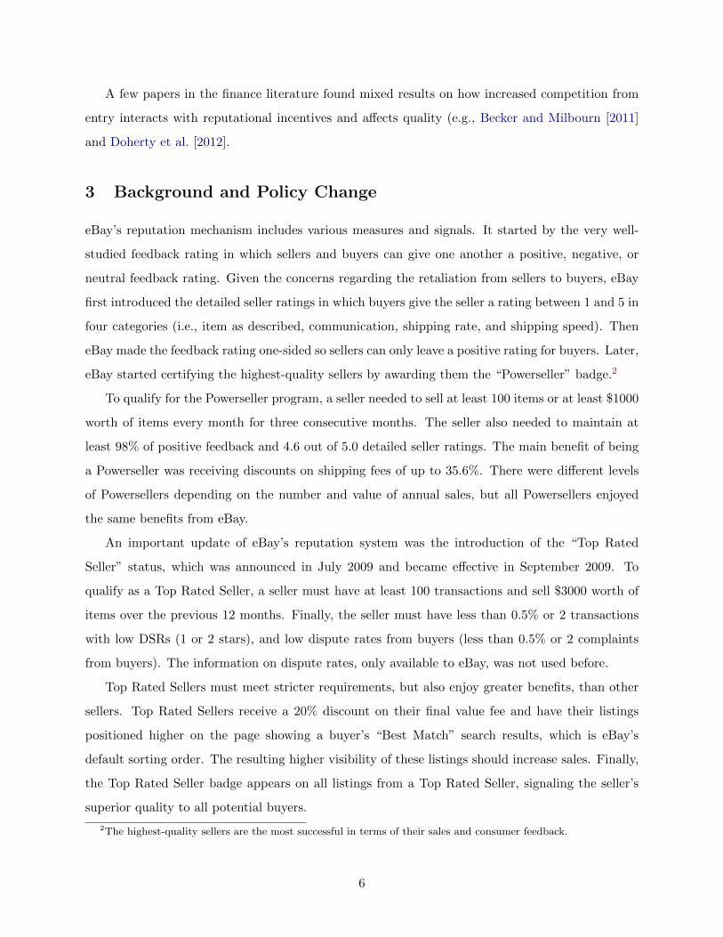
meaningful implications for the entrant cohorts. Figure 3 reports the correlation between the size

of the entrant cohort and the share of badged sellers in each subcategory. Given the change in both

size of entrant cohort and share of badged sellers, to be able to compare the results before and after

the policy change, we need to normalize the two. To do so, we rank subcategories in both metrics

each month and assign the percentile they are at to the subcategory. Figure 3 shows that there is

indeed a negative correlation between the number of entrants and the share of badged sellers across

subcategories (e.g., the higher the share of badged sellers in a subcategory, the smaller the size of

11

Figure 3: Market Structure and Entry

the entrant cohort in that subcategory). This negative correlation is present even before the policy

change, but it becomes stronger after the policy change (following the dashed line), suggesting a

variation in the entry pattern.

First, we would like to quantify the impact of the policy change on the number of entrants.

To further study the impact of the policy change on the number of entrants, we look at regression

1. Table 1 reports γ̂ from regression 1 for four outcome variables. To normalize across categories,

we use the entrants’ ratio Entrant Ratioct, which is defined as “flow over stock”: the number of

entrants divided by the number of incumbents (sellers who listed in t − 1) in subcategory c in

month t. We see in Panel A of Table 1 that the impact of the policy change is about -30% in the

six-month window (data from three months before and three months after the policy change). We

interpret this result as follows: a 10% larger decrease in the share of badged sellers leads to 3%

more entrants. The impact of the policy change decreases to -20% if we expand our window length

to 12 months. This lower estimate shows that the marginal impact from month 4 to month 6 is

smaller than that from month 1 to month 3. In column 3, we compare categories 7 to 12 months

after the policy change to capture long term effect of the policy.4 The result show that the marginal

impact of policy becomes -4.7% and is not statistically significant. These results suggest that the

impact shrinks dramatically in a year and stabilizes towards a new steady state after six months.

To observe the differential impact of the policy change on the number of entrants, we illustrate

its impact on the top and bottom 20 percentiles of the affected subcategories as determined by

regression 1, β̂c. Figure 4a shows that in the top 20 percentile of categories, the share of badged

sellers decreases from about 35% to less than 15% after the policy change, whereas in the bottom

20 percentile, the share of badged sellers decreases from about 18% to 10%. There is no obvious

variation in the number of entrants for the bottom 20 percentiles of subcategories, whereas the

4We do not include longer time periods, as eBay has made significant changes to their trust mechanism.

12

average number of entrants to the top 20 percentiles has increased by 25%. Additionally, entry

rates seem to stabilize after three months.

7.2 Average Performance of the Entrant Cohort

Now, we study how the performance, or quality, of the entrant cohort is affected by this policy

change. We look at three measures of performance: effective percentage positive (EPP), the average

sales’ quantity, and the survival rate.

First, we study the effective percentage positive (EPP), the number of positive feedback trans-

actions divided by the number of total transactions over a given period. Nosko and Tadelis [2015]

show that EPP contains more information on transaction quality than conventional feedback rat-

ings. Specifically, we define a seller’s EPP using the number of transactions and positive feedbacks

in the first year of entry, conditional on the entrant’s survival (i.e., selling at least one item) in the

second year. We condition both measures on survival in the second year to eliminate the survival

effect. We have also tried alternative definition of EPPs and also without conditioning on survival

of sellers, and the results are reported in section 8 and show similar patterns.

Panel B in Table 1 shows that there is an increase in entrants’ average quality in the more

affected subcategories, as measured by the EPP, after the policy change. This effect stabilizes from

-10% to -6.6% as we expand the window length from six to twelve months. Column 3 shows that the

increase in EPP persists from the seventh to the twelfth month after the policy change, suggesting

that its quality effect is persistent over longer time period.

Figure 4b shows the average EPP for entrants in the top and bottom 20 percentiles of the

affected subcategories. Note that EPPs are decreasing on eBay over time, but the average EPP is

higher for the top 20 percentile of the affected subcategories compared to the bottom 20 percentile

of subcategories.

Second, we look at the sales quantity during a seller’s first year of entry, conditional on entrant’s

survival in the second year. Positive and significant coefficient in column 1 of Panel C shows that

over the short term, sales quantity from the entrants is smaller in subcategories affected more by

the policy change; however, this drop becomes insignificant when considering longer time period.

Additionally, from the seventh to the twelfth month after the policy change, the change in the

entrants’ sales quantity remains statistically insignificant. This result indicates that the average

entrant is smaller in the subcategories most affected by the policy change. Recall that these

categories have more entrants on average as well. As a result, this regression does not necessary

13

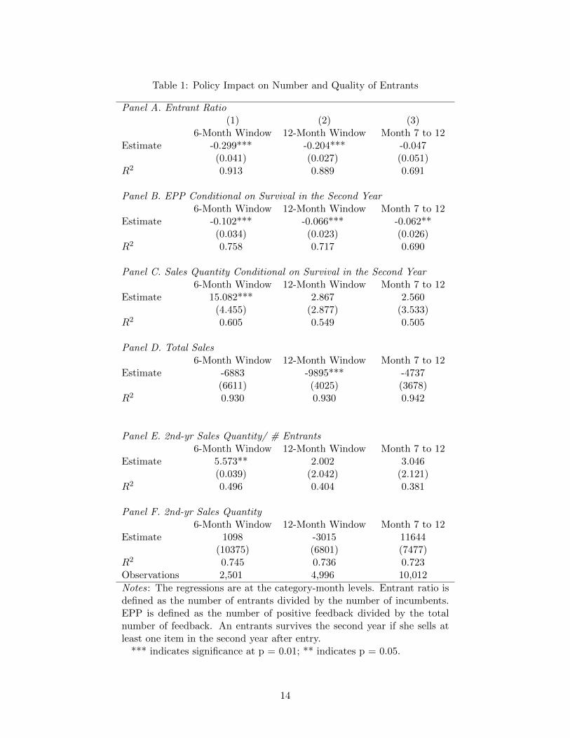
Table 1: Policy Impact on Number and Quality of Entrants

Panel A. Entrant Ratio(1) (2) (3)

6-Month Window 12-Month Window Month 7 to 12Estimate -0.299*** -0.204*** -0.047

(0.041) (0.027) (0.051)R2 0.913 0.889 0.691

Panel B. EPP Conditional on Survival in the Second Year6-Month Window 12-Month Window Month 7 to 12

Estimate -0.102*** -0.066*** -0.062**(0.034) (0.023) (0.026)

R2 0.758 0.717 0.690

Panel C. Sales Quantity Conditional on Survival in the Second Year6-Month Window 12-Month Window Month 7 to 12

Estimate 15.082*** 2.867 2.560(4.455) (2.877) (3.533)

R2 0.605 0.549 0.505

Panel D. Total Sales6-Month Window 12-Month Window Month 7 to 12

Estimate -6883 -9895*** -4737(6611) (4025) (3678)

R2 0.930 0.930 0.942

Panel E. 2nd-yr Sales Quantity/ # Entrants6-Month Window 12-Month Window Month 7 to 12

Estimate 5.573** 2.002 3.046(0.039) (2.042) (2.121)

R2 0.496 0.404 0.381

Panel F. 2nd-yr Sales Quantity6-Month Window 12-Month Window Month 7 to 12

Estimate 1098 -3015 11644(10375) (6801) (7477)

R2 0.745 0.736 0.723Observations 2,501 4,996 10,012

Notes: The regressions are at the category-month levels. Entrant ratio isdefined as the number of entrants divided by the number of incumbents.EPP is defined as the number of positive feedback divided by the totalnumber of feedback. An entrants survives the second year if she sells atleast one item in the second year after entry.

*** indicates significance at p = 0.01; ** indicates p = 0.05.

14

Figure 4: Policy Impact on Entrants

(a) Policy Impact on Number of Entrants

(b) Policy Impact on EPP

(c) Policy Impact on Sales

Notes: The vertical axis on the right shows the share of badged sellers, and the one on the left shows thenormalized number of entrants. The numbers of entrants in the six-month period before the policy changeare normalized to 100. The figure on the left is for the top 20 percentile of the affected subcategories andthe one on the right is for the bottom 20 percentile of the affected subcategories.

15

imply a decrease in the total number of sales by entrants. In fact, when we run a regression of sales

by entrants, as indicated by Panel D in Table 1, we observe that the subcategories more affected by

the policy change have a higher total number of sales by entrants. Additionally, we plot analogous

graphs to analyze sales by the top and bottom 20 percentiles of the affected subcategories in Figure

4c, which shows a short-run surge in the number of total sales in the top 20 percentile of the affected

subcategories with very little impact on the bottom 20 percentile of the affected subcategories.

Finally, we study entrants’ survival by looking at the average size of entrants a year after entry,

with giving 0 to sellers who do not sell any items in their second year. The advantage of this measure

over a simple survival dummy is that it is able to capture a seller’s change in size as well as seller’s

exit.5 Panel E shows that the average sales quantity in the second year per entrant decreases more

for entrants in categories that are more affected by the policy change. This observation is consistent

with the fact that the entrants tend to be smaller in the affected area as shown in Panel C. However,

this effect does not stay significant when we consider longer time period or if we consider 7 to 12

months after the policy change. Additionally, the total number of items sold by entrants in the

second year does not change significantly, as shown in Panel F.

7.3 Quality Distribution of Entrant Cohort

An important test for our simple theory is how the distribution of entrants’ quality varies after the

policy change. The theory predicted that under mild assumptions, there should be more entrants

of high quality, as being high-quality becomes more rewarding. Additionally, the theory predicted

that sellers of low quality may enter more often if pooling with a better set of sellers would imply

lower-quality sellers can receive higher average prices in equilibrium. To test this prediction, within

each subcategories, we look at different deciles of sellers. For example, we look at entrants within

the top 10 percentile as determined by their EPP score. Then we check if these EPPs have increased

more for the subcategories more affected by the policy change. A positive number will indicate

a fatter tail of the distribution on the right. Respectively, if we look at the bottom 10 percentile

of entrants in terms of their EPP and compare the subcategories, a negative number means a

fatter tail on the left. Another prediction was that the sellers who had a chance of becoming

badged before and no longer have this opportunity after the policy change will enter less often.

A distribution of entrants’ quality with a fatter tail from both left and right will indicate a fewer

5Another method to study the survival rate is to have a dummy variable equal to zero if the seller does not sellany item in the second year. However, we believe that is not a very good measure, as many sellers, even if they quitselling professionally on eBay, may still sell occasionally on the platform.

16

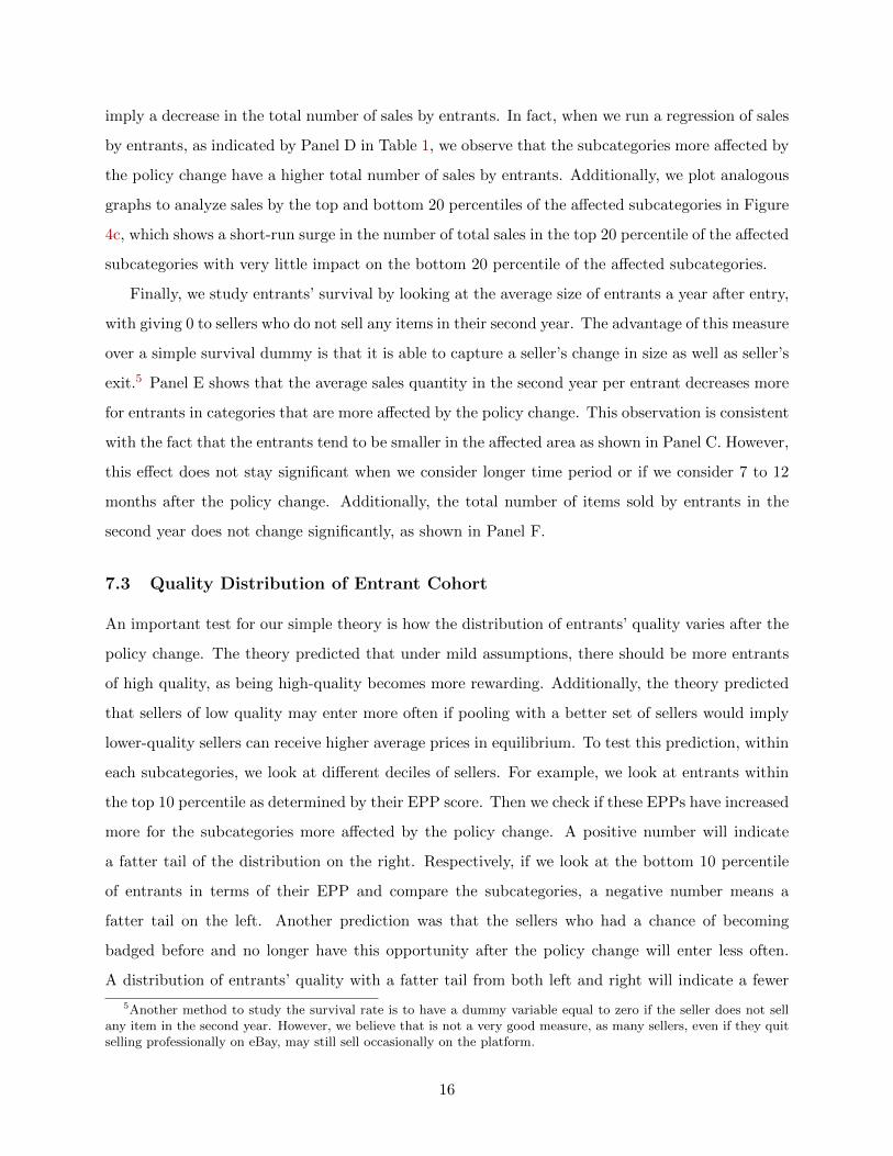
Figure 5: Change in EPP for Entrants in Different Quality Deciles

Notes: Bars indicate 95% confidence intervals.

share of average-quality entrants.

We plot the change in EPP for entrants of different quality deciles in Figure 5. EPPs are com-

puted based on the number of transactions in the first three years after entry. For consistency, we

condition the EPP calculation on an entrant’s survival in the second year. Entrants are counted ev-

ery two months. To be able to take the average of cohorts, we restrict our attention to subcategories

with at least 100 entrants. As a result, for each subcategory, we have three observations (six-month

equivalent) before the policy change and three observations after it. Additionally, we only consider

subcategories that have entry in all of the six two-month periods and remove subcategories with a

small number of entrants. This leaves us with 228 out of the 400 subcategories.

The x-axis in Figure 5 indicates different quality deciles, with “10” being the lowest decile of

EPP and “1” being the highest decile of EPP. The dots are point estimates of the changes in EPP for

the entrant cohorts, and the bars are 95% confidence intervals. Although only a couple of the point

estimates are statistically different from 0, we observe a monotonically increasing relationship that

is consistent with our prediction that the quality distribution of entrants after the policy change

varies and has fatter tails because sellers from the extremes of the quality distribution now have

stronger incentives to enter.

17

7.4 Impact on Incumbents

The results in the previous subsections show that the policy change had an impact on the entry

decision of sellers into different subcategories, and that this impact differed among entrants selling

different quality levels, suggesting a selection-of-entrants interpretation. However, the impact on

the quality sold by entrants could in principle be solely driven by a moral-hazard story, where

similar entrants changed their behavior after the policy change depending on the subcategory they

entered. Figure 6 plots the average EPP of all entrants and incumbents within six months of the

policy change. As indicated in the figure, the average EPP of entrants has increased, while no

apparent change in the average EPP of incumbents is observed. However, we might not observe

any significant change in the average EPP of the incumbents, but there would be a change in the

distribution of incumbents’ quality.

To address this concern, we study the behavior of different types of incumbent sellers. In Figure

7a, we plot the average monthly EPP for incumbents with different badging status. There are four

groups of incumbents, with all possible combinations of their badging status before and after the

policy change. We only show the incumbents that were never badged and those who were always

badged; for the other two groups, we observe similar results. In particular, there is no obvious

difference between the incumbents’ EPP in 2009 (the year of the policy change) and their EPP in

2008 and 2010. This suggests that the change in the average monthly EPP observed in these two

figures is due to seasonality.

We created a similar plot for sellers of different quality quartiles. We again note that there

is no observable change in incumbents’ EPP after the policy change after removing seasonality.

Thus, the incumbents do not seem to change their behavior in response to the policy change. This

observation suggests that the increase in quality provided by entrants at the tails of the quality

distribution is more likely due to improved selection rather than to behavioral changes.

7.5 Impact on Badge Premium

We study how badge premiums change for the four groups of sellers: BB, BN , NB, NN , where

B indicates that the seller is badged and N indicates that the seller is not badged. We use the BB

group as an example to illustrate how these groups are defined: 1) We find if a seller is badged

for a given month. 2) A seller belongs to the BB group if she is a Powerseller for at least 91.6%

of her active months on eBay before the policy change (eleven out of twelve months) and is eTRS

18

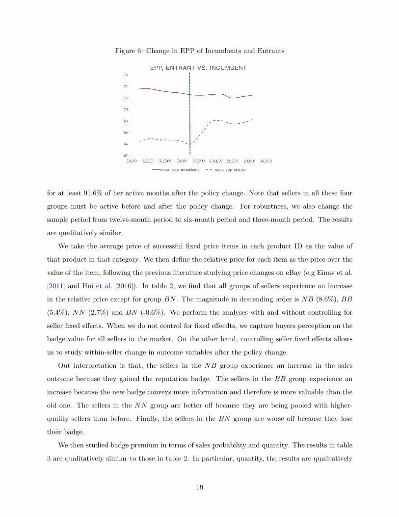
Figure 6: Change in EPP of Incumbents and Entrants

for at least 91.6% of her active months after the policy change. Note that sellers in all these four

groups must be active before and after the policy change. For robustness, we also change the

sample period from twelve-month period to six-month period and three-month period. The results

are qualitatively similar.

We take the average price of successful fixed price items in each product ID as the value of

that product in that category. We then define the relative price for each item as the price over the

value of the item, following the previous literature studying price changes on eBay (e.g Einav et al.

[2011] and Hui et al. [2016]). In table 2, we find that all groups of sellers experience an increase

in the relative price except for group BN . The magnitude in descending order is NB (8.6%), BB

(5.4%), NN (2.7%) and BN (-0.6%). We perform the analyses with and without controlling for

seller fixed effects. When we do not control for fixed effecdts, we capture buyers perception on the

badge value for all sellers in the market. On the other hand, controlling seller fixed effects allows

us to study within-seller change in outcome variables after the policy change.

Out interpretation is that, the sellers in the NB group experience an increase in the sales

outcome because they gained the reputation badge. The sellers in the BB group experience an

increase because the new badge conveys more information and therefore is more valuable than the

old one. The sellers in the NN group are better off because they are being pooled with higher-

quality sellers than before. Finally, the sellers in the BN group are worse off because they lose

their badge.

We then studied badge premium in terms of sales probability and quantity. The results in table

3 are qualitatively similar to those in table 2. In particular, quantity, the results are qualitatively

19

Figure 7: Change in EPP of Incumbents

(a) Badged Vs. Non-Badged

(b) Top Vs. Bottom 20 Percentile

Notes: The solid lines correspond to EPPs in the year when the policy change took place (2009). The dashedlines and the dashed-dotted lines are for EPPs in the year before and year after the policy year, respectively.The x-axis indicates months, and its interaction with the vertical dotted line is 12.

20

Table 2: Change in Badge Premium: Relative Price

6M Win 4M Win 2M Win 6M Win 4M Win 2M WinBB*Pol 0.027*** 0.018*** 0.017*** 0.001 0.014*** 0.014***

(0.002) (0.003) (0.003) (0.002) (0.002) (0.003)BN*Pol -0.033*** -0.018*** -0.009*** -0.015*** 0.014*** 0.014***

(0.002) (0.002) (0.002) (0.002) (0.002) (0.002)NB*Pol 0.059*** 0.051*** -0.005 0.014* 0.009 0.017*

(0.008) (0.010) (0.011) (0.009) (0.008) (0.010)Seller FE X X XR2 0.004 0.004 0.006 0.944 0.971 0.955

Benchmark Change in NN GroupPol 0.027*** 0.032*** 0.005 0.026*** -0.016*** -0.028***

(0.008) (0.004) (0.004) (0.008) (0.004) (0.004)Seller FE X X XNotes: We also control for BB, BN , and NB, and week dummies. The bench-mark changes for the NN group are displayed in the second panel. The estima-tion on benchmark cases also controls for log(Price), week dummies, and theconstant term. B indicates that the seller is badged and N indicates that theseller is not badged. The first letter refers to the the seller’s status before thepolicy change, and the second letter refers to the seller’s status after the policychange.

*** indicates significance at p = 0.01; ** indicates p = 0.05 ; * indicates p = 0.1.

similar, and the magnitude of changes in descending order is NB, BB, NN , and BN .

7.6 Impact on Market Shares

In this section, we analyze the policy impact on market share for different groups of sellers. We

define market share based on sellers’ transactions in one-month or three-month intervals. We use

three months so that the market share of entrants is not too small.

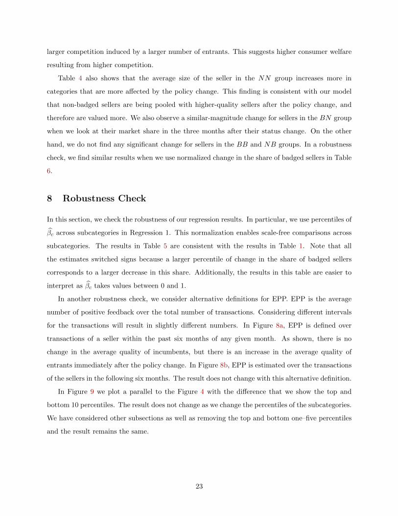
Panel A in Table 4 shows that the market share of entrants as a whole is larger in categories

that are more affected by the policy change: a 10% larger decrease in share of badged seller leads to

an increase in market share for entrants by 0.49% and 2.25%, respectively, depending on whether

we calculate market share based on one-month or three-month intervals. Relatedly, Panel B shows

that the average size of entrants is smaller in categories that are more affected by the policy change:

a 10% larger decrease in share of badged seller leads to an decrease in market share for entrants

by 0.08% and 0.03%, respectively, depending on the window length for defining market share.

These two results together show that entrants as a whole are grabbing a larger market share as

their quality has increased after the policy change, but each individual entrant is smaller due to

21

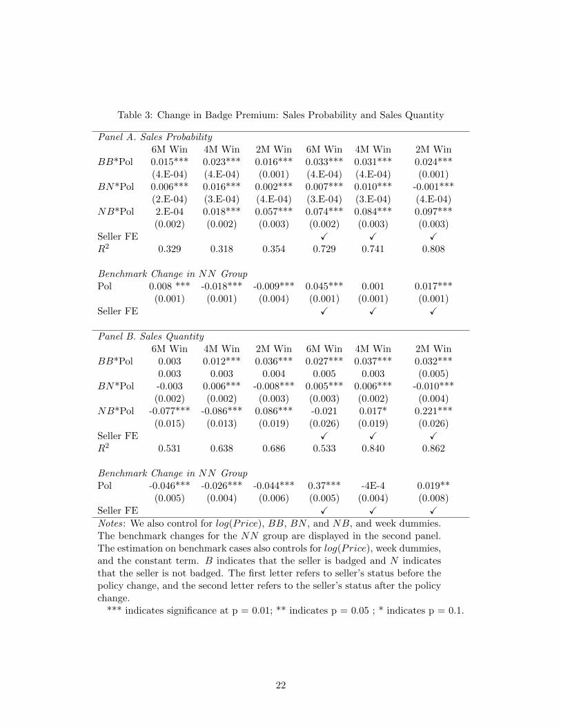
Table 3: Change in Badge Premium: Sales Probability and Sales Quantity

Panel A. Sales Probability6M Win 4M Win 2M Win 6M Win 4M Win 2M Win

BB*Pol 0.015*** 0.023*** 0.016*** 0.033*** 0.031*** 0.024***(4.E-04) (4.E-04) (0.001) (4.E-04) (4.E-04) (0.001)

BN*Pol 0.006*** 0.016*** 0.002*** 0.007*** 0.010*** -0.001***(2.E-04) (3.E-04) (4.E-04) (3.E-04) (3.E-04) (4.E-04)

NB*Pol 2.E-04 0.018*** 0.057*** 0.074*** 0.084*** 0.097***(0.002) (0.002) (0.003) (0.002) (0.003) (0.003)

Seller FE X X XR2 0.329 0.318 0.354 0.729 0.741 0.808

Benchmark Change in NN GroupPol 0.008 *** -0.018*** -0.009*** 0.045*** 0.001 0.017***

(0.001) (0.001) (0.004) (0.001) (0.001) (0.001)Seller FE X X X

Panel B. Sales Quantity6M Win 4M Win 2M Win 6M Win 4M Win 2M Win

BB*Pol 0.003 0.012*** 0.036*** 0.027*** 0.037*** 0.032***0.003 0.003 0.004 0.005 0.003 (0.005)

BN*Pol -0.003 0.006*** -0.008*** 0.005*** 0.006*** -0.010***(0.002) (0.002) (0.003) (0.003) (0.002) (0.004)

NB*Pol -0.077*** -0.086*** 0.086*** -0.021 0.017* 0.221***(0.015) (0.013) (0.019) (0.026) (0.019) (0.026)

Seller FE X X XR2 0.531 0.638 0.686 0.533 0.840 0.862

Benchmark Change in NN GroupPol -0.046*** -0.026*** -0.044*** 0.37*** -4E-4 0.019**

(0.005) (0.004) (0.006) (0.005) (0.004) (0.008)Seller FE X X XNotes: We also control for log(Price), BB, BN , and NB, and week dummies.The benchmark changes for the NN group are displayed in the second panel.The estimation on benchmark cases also controls for log(Price), week dummies,and the constant term. B indicates that the seller is badged and N indicatesthat the seller is not badged. The first letter refers to seller’s status before thepolicy change, and the second letter refers to the seller’s status after the policychange.

*** indicates significance at p = 0.01; ** indicates p = 0.05 ; * indicates p = 0.1.

22

larger competition induced by a larger number of entrants. This suggests higher consumer welfare

resulting from higher competition.

Table 4 also shows that the average size of the seller in the NN group increases more in

categories that are more affected by the policy change. This finding is consistent with our model

that non-badged sellers are being pooled with higher-quality sellers after the policy change, and

therefore are valued more. We also observe a similar-magnitude change for sellers in the BN group

when we look at their market share in the three months after their status change. On the other

hand, we do not find any significant change for sellers in the BB and NB groups. In a robustness

check, we find similar results when we use normalized change in the share of badged sellers in Table

6.

8 Robustness Check

In this section, we check the robustness of our regression results. In particular, we use percentiles of

β̂c across subcategories in Regression 1. This normalization enables scale-free comparisons across

subcategories. The results in Table 5 are consistent with the results in Table 1. Note that all

the estimates switched signs because a larger percentile of change in the share of badged sellers

corresponds to a larger decrease in this share. Additionally, the results in this table are easier to

interpret as β̂c takes values between 0 and 1.

In another robustness check, we consider alternative definitions for EPP. EPP is the average

number of positive feedback over the total number of transactions. Considering different intervals

for the transactions will result in slightly different numbers. In Figure 8a, EPP is defined over

transactions of a seller within the past six months of any given month. As shown, there is no

change in the average quality of incumbents, but there is an increase in the average quality of

entrants immediately after the policy change. In Figure 8b, EPP is estimated over the transactions

of the sellers in the following six months. The result does not change with this alternative definition.

In Figure 9 we plot a parallel to the Figure 4 with the difference that we show the top and

bottom 10 percentiles. The result does not change as we change the percentiles of the subcategories.

We have considered other subsections as well as removing the top and bottom one–five percentiles

and the result remains the same.

23

Table 4: Change in Market Share for Different Groups

Panel A. Change in Market Share for Different GroupsMarket Share Based on One-Month Intervals

Entrants BB BN NB NNEstimate -0.049*** 0.727*** -0.170*** -0.059*** -0.559***

(0.019) (0.035) (0.023) (0.017) (0.035)R2 0.825 0.882 0.843 0.439 0.801Observations 5129 5129 4776 4902 5151

Market Share Based on Three-Month IntervalsEntrants BB BN NB NN

Estimate -0.225*** 1.854*** -0.509*** -0.258*** -1.803***(0.075) (0.644) (0.069) (0.082) (0.158)

R2 0.525 0.435 0.797 0.728 0.778Observations 4710 5113 4979 5072 5157

Panel B. Change in Average Seller Size for Different GroupsMarket Share Based on One-Month Intervals

Entrants BB BN NB NNEstimate 0.008** 0.004 -0.007 -0.002 -0.009**

(0.003) (0.004) (0.008) (0.006) (0.004)R2 0.572 0.958 0.323 0.412 0.738

Market Share Based on Three-Month IntervalsEntrants BB BN NB NN

Estimate 0.003** 0.004 -0.009** -0.005 -0.008***(0.001) (0.002) (0.004) (0.004) (0.003)

R2 0.582 0.989 0.411 0.596 0.668

Notes: We use data from six months before and six months after thepolicy change. Definition of the four groups are defined in the text.Market shares are defined based on sellers’ sales in one month or threemonths .

*** indicates significance at p = 0.01; ** indicates p = 0.05.

24

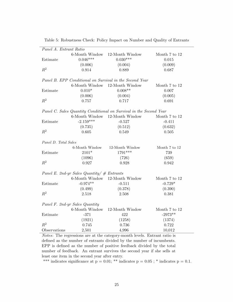
Table 5: Robustness Check: Policy Impact on Number and Quality of Entrants

Panel A. Entrant Ratio6-Month Window 12-Month Window Month 7 to 12

Estimate 0.046*** 0.030*** 0.015(0.006) (0.004) (0.009)

R2 0.914 0.889 0.687

Panel B. EPP Conditional on Survival in the Second Year6-Month Window 12-Month Window Month 7 to 12

Estimate 0.010* 0.008** 0.007(0.006) (0.004) (0.005)

R2 0.757 0.717 0.691

Panel C. Sales Quantity Conditional on Survival in the Second Year6-Month Window 12-Month Window Month 7 to 12

Estimate -2.159*** -0.527 -0.411(0.735) (0.512) (0.632)

R2 0.605 0.549 0.505

Panel D. Total Sales

6-Month Window 12-Month Window Month 7 to 12

Estimate 2101* 1791*** 739(1096) (726) (659)

R2 0.927 0.928 0.942

Panel E. 2nd-yr Sales Quantity/ # Entrants6-Month Window 12-Month Window Month 7 to 12

Estimate -0.974** -0.511 -0.729*(0.499) (0.378) (0.390)

R2 2.518 2.508 0.381

Panel F. 2nd-yr Sales Quantity6-Month Window 12-Month Window Month 7 to 12

Estimate -371 422 -2973**(1921) (1258) (1374)

R2 0.745 0.736 0.722Observations 2,501 4,996 10,012

Notes: The regressions are at the category-month levels. Entrant ratio isdefined as the number of entrants divided by the number of incumbents.EPP is defined as the number of positive feedback divided by the totalnumber of feedback. An entrant survives the second year if she sells atleast one item in the second year after entry.*** indicates significance at p = 0.01; ** indicates p = 0.05 ; * indicates p = 0.1.

25

Figure 8: Robustness: Change in EPP of Incumbents and Entrants

(a) (b)

Notes: In definition 3, EPP is calculated with transactions from six months before the policy change. Indefinition 4, EPP is calculated with transactions from six months after the policy change.

Table 6: Change in Market Share for Different Groups

Change in Seller Size for Different GroupsMarket Share Based on One-Month Intervals

Entrants BB BN NB NNEstimate 0.000 -0.001* 0.000 0.000 0.003***

(0.001) (0.001) (0.001) (0.001) (0.001)R2 0.581 0.950 0.384 0.420 0.741

Observations 5129 5129 4776 4902 5151

Market Share Based on Three-Month IntervalsEntrants BB BN NB NN

Estimate 0.000 -0.001*** -0.001 0.001 0.003***(0.000) (0.000) (0.001) (0.001) (0.001)

R2 0.547 0.985 0.512 0.670 0.743

Observations 5138 5113 4979 5072 5157

Notes: Definition of the four groups are given in the text.*** indicates significance at p = 0.01.

26

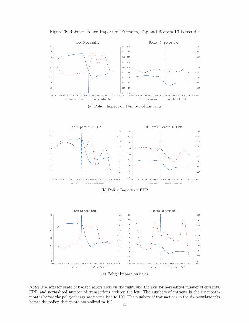
Figure 9: Robust: Policy Impact on Entrants, Top and Bottom 10 Percentile

(a) Policy Impact on Number of Entrants

(b) Policy Impact on EPP

(c) Policy Impact on Sales

Notes:The axis for share of badged sellers areis on the right, and the axis for normalized number of entrants,EPP, and normalized number of transactions areis on the left. The numbers of entrants in the six month-months before the policy change are normalized to 100. The numbers of transactions in the six monthmonthsbefore the policy change are normalized to 100.

27

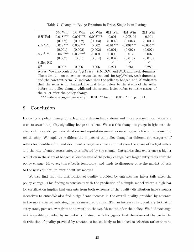
Table 7: Change in Badge Premium in Price, Single-Item Listings

6M Win 4M Win 2M Win 6M Win 4M Win 2M WinBB*Pol 0.018*** 0.007*** 0.008*** 0.001 4.20E-06 -0.001

(0.002) (0.002) (0.003) (0.002) (0.002) (0.003)BN*Pol 0.012*** 0.008*** 0.002 -0.01*** -0.007*** -0.005**

(0.001) (0.002) (0.002) (0.001) (0.002) (0.002)NB*Pol 0.055*** 0.035*** -0.001 0.009 0.012 0.007

(0.007) (0.01) (0.014) (0.007) (0.010) (0.013)Seller FE X X XR2 0.007 0.006 0.006 0.271 0.261 0.289

Notes: We also control for log(Price), BB, BN , and NB, and week dummies.The estimation on benchmark cases also controls for log(Price), week dummies,and the constant term. B indicates that the seller is badged and N indicatesthat the seller is not badged.The first letter refers to the status of the sellerbefore the policy change, whileand the second letter refers to itsthe status ofthe seller after the policy change.

*** indicates significance at p = 0.01; ** for p = 0.05 ; * for p = 0.1.

9 Conclusion

Following a policy change on eBay, more demanding criteria and more precise information are

used to award a quality-signalling badge to sellers. We use this change to gauge insight into the

effects of more stringent certification and reputation measures on entry, which is a hard-to-study

relationship. We exploit the differential impact of the policy change on different subcategories of

sellers for identification, and document a negative correlation between the share of badged sellers

and the rate of entry across categories affected by the change. Categories that experience a higher

reduction in the share of badged sellers because of the policy change have larger entry rates after the

policy change. However, this effect is temporary, and tends to disappear once the market adjusts

to the new equilibrium after about six months.

We also find that the distribution of quality provided by entrants has fatter tails after the

policy change. This finding is consistent with the prediction of a simple model where a high bar

for certification implies that entrants from both extremes of the quality distribution have stronger

incentives to enter.We also find a significant increase in the overall quality provided by entrants

in the more affected subcategories, as measured by the EPP, an increase that, contrary to that of

entry rates, persists even from the seventh to the twelfth month after the policy. We find nochange

in the quality provided by incumbents, instead, which suggests that the observed change in the

distribution of quality provided by entrants is indeed likely to be linked to selection rather than to

28

Table 8: Change in Badge Premium in Sales Probability and Quantity, Single-Item Listings

Panel A. Sales Probability6M Win 4M Win 2M Win 6M Win 4M Win 2M Win

BB*Pol 0.023*** 0.025*** 0.016*** 0.038*** 0.032*** 0.021***(5.E-04) (5.E-04) (0.001) (0.001) (0.001) (0.001)

BN*Pol 0.006*** 0.012*** 0.002*** 0.006*** 0.012*** 0.004***(3.E-04) (4.E-04) (0.001) (4.E-04) (4.E-04) (0.001)

NB*Pol 0.006*** 0.031*** 0.064*** 0.108*** 0.129*** 0.125***(0.002) (0.003) (0.004) (0.003) (0.004) (0.005)

Seller FE X X XR2 0.379 0.364 0.408 0.788 0.797 0.849

Panel B. Sales Quantity6M Win 4M Win 2M Win 6M Win 4M Win 2M Win

BB*Pol 0.016*** 0.021*** 0.014*** 0.032*** 0.031*** 0.020***(5.E-04) (5.E-04) (0.001) (0.001) (0.001) (0.001)

BN*Pol 0.007*** 0.012*** 0.003*** 0.005*** 0.011*** 0.004***(3.E-04) (4.E-04) (0.001) (4.E-04) (4.E-04) (0.001)

NB*Pol 0.019*** 0.043*** 0.069*** 0.105*** 0.126*** 0.125***(0.002) (0.003) (0.004) (0.003) (0.004) (0.005)

Seller FE X X XR2 0.367 0.352 0.398 0.776 0.786 0.841

Notes: We also control for log(Price), BB, BN , and NB, and week dummies.The estimation on benchmark cases also controls for log(Price), week dummies,and the constant term. B indicates that the seller is badged and N indicatesthat the seller is not badged.The first letter refers to the status of the sellerbefore the policy change, whileand the second letter refers to itsthe status ofthe seller after the policy change.

*** indicates significance at p = 0.01; ** for p = 0.05 ; * for p = 0.1.

29

a change in entrants’ behavior. These results indicate that the availability and precision of past

performance information are important not only for the rate of entry in a market, but also for the

quality of who is actually entering hence for how markets evolve in the long run. This finding has

direct implications for the design of reputation and certification mechanisms in electronic and other

markets plagued by information asymmetries, including public procurement markets.

References

Patrick Bajari and Ali Hortacsu. Economic insights from internet auctions. Journal of Economic

Literature, 42(2):457–486, 2004.

Bo Becker and Todd Milbourn. How did increased competition affect credit ratings? Journal of

Financial Economics, 101(3):493–514, 2011.

Jeffrey V Butler, Enrica Carbone, Pierluigi Conzo, and Giancarlo Spagnolo. Reputation and entry

in procurement. 2013.

Chrysanthos Dellarocas, Federico Dini, and Giancarlo Spagnolo. Designing reputation (feedback)

mechanisms. 2006.

Neil A Doherty, Anastasia V Kartasheva, and Richard D Phillips. Information effect of entry into

credit ratings market: The case of insurers’ ratings. Journal of Financial Economics, 106(2):

308–330, 2012.

Liran Einav, Theresa Kuchler, Jonathan D Levin, and Neel Sundaresan. Learning from seller

experiments in online markets. Technical report, National Bureau of Economic Research, 2011.

Daniel W Elfenbein, Raymond Fisman, and Brian McManus. Market structure, reputation, and

the value of quality certification. American Economic Journal: Microeconomics, 7(4):83–108,

2015.

Hugo Hopenhayn and Maryam Saeedi. Reputation signals and market outcomes. Technical report,

National Bureau of Economic Research, 2016.

Xiang Hui. E-commerce platforms and international trade: A large-scale field experiment. Available

at SSRN 2663805, 2017.

30

Xiang Hui, Maryam Saeedi, Zeqian Shen, and Neel Sundaresan. Reputation and regulations:

evidence from ebay. Management Science, 62(12):3604–3616, 2016.

Benjamin Klein and Keith B Leffler. The role of market forces in assuring contractual performance.

Journal of political Economy, 89(4):615–641, 1981.

Tobias J Klein, Christian Lambertz, and Konrad O Stahl. Market transparency, adverse selection,

and moral hazard. Journal of Political Economy, 124(6):1677–1713, 2016.

Chris Nosko and Steven Tadelis. The limits of reputation in platform markets: An empirical

analysis and field experiment. Technical report, National Bureau of Economic Research, 2015.

Maryam Saeedi, Zeqian Shen, and Neel Sundaresan. The value of feedback: An analysis of reputa-

tion system. Ohio State University, working paper, 2013.

Giancarlo Spagnolo. Reputation, competition, and entry in procurement. International Journal of

Industrial Organization, 30(3):291–296, 2012.

Steven Tadelis. Reputation and feedback systems in online platform markets. Annual Review of

Economics, 8:321–340, 2016.

APPENDIX

31