Probing Asphaltenes Aggregation with Fluorescence Techniques

by

Hui Ting Zhang B.Sc., University of Victoria, 2008

A Thesis Submitted in Partial Fulfillment of the Requirements for the Degree of

MASTER OF SCIENCE

in the Department of Chemistry

© Hui Ting Zhang, 2010 University of Victoria

All rights reserved. This thesis may not be reproduced in whole or in part, by photocopy

or other means, without the permission of the author.

ii

Supervisory Committee

Probing Asphaltene Aggregation with Fluorescence Techniques

by

Hui Ting Zhang B.Sc., University of Victoria, 2008

Supervisory Committee Dr. Cornelia Bohne (Department of Chemistry) Supervisor Dr. Matthew Moffitt (Department of Chemistry) Departmental Member Dr. David Sinton (Department of Mechanical Engineering) Outside Member

iii

Abstract

Supervisory Committee Dr. Cornelia Bohne (Department of Chemistry) Supervisor Dr. Matthew Moffitt (Department of Chemistry) Departmental Member Dr. David Sinton (Department of Mechanical Engineering) Outside Member

Asphaltenes correspond to the fraction of oil that is insoluble in heptane but is

soluble in toluene. The aggregates of asphaltene are of interest because they cause serious

problems in the production of oil. Asphaltenes contain fluorescent moieties, and as such

they can be studied by fluorescence techniques.

The first objective of this work was to develop methodologies to study the

fluorescence of asphaltenes, and to investigate the fluorescence of asphaltenes at various

concentrations. Time-resolved fluorescence studies indicate that asphaltenes have

different chromophores with different lifetimes. The average lifetime of the asphaltene

emission decreased when the asphaltene concentration was increased because of

quenching processes occurring within the aggregates. The measurement of lifetimes at

different excitation and emission wavelengths demonstrated that different components of

asphaltene aggregate at different concentrations.

The second objective of this work was to investigate how accessible the

asphaltene aggregate is to small molecules by fluorescence quenching experiments.

Nitromethane was the quencher used in the fluorescence of asphaltenes. The quenching

efficiencies were found to be independent of the concentration of asphaltenes. However,

the quenching efficiencies differed for different chromophores, suggesting a selective

iv quenching for nitromethane of the excited states for the different chromophores of

asphaltenes.

The third objective of this thesis was to investigate the fluorescence of externally

added probes that might be incorporated in asphaltene aggregates through π−π stacking.

Pyrene was chosen as the probe because its fluorescence properties are strongly affected

by its surroundings. The pyrene emission was quenched by nitromethane. The quenching

efficiencies determined for pyrene in the absence or the presence of asphaltene

aggregates were the same. This suggests that pyrene is located in an open environment,

where the asphaltene aggregates do not offer any protection for pyrene from

nitromethane.

v

Table of Contents

PRELIMINARY PAGES

Supervisory Committee ...................................................................................................... ii

Abstract .............................................................................................................................. iii

Table of Contents ................................................................................................................ v

List of Tables ................................................................................................................... viii

List of Figures ..................................................................................................................... x

List of Schemes ................................................................................................................ xvi

List of Abbreviations ...................................................................................................... xvii

Acknowledgments ............................................................................................................. xx

Dedication ........................................................................................................................ xxi

1. INTRODUCTION ....................................................................................................... 1

1.1 Asphaltenes ............................................................................................................... 1 1.1.1 The importance of asphaltenes ........................................................................... 1 1.1.2 Definition and composition of asphaltenes ........................................................ 2 1.1.3 Asphaltene aggregates ....................................................................................... 5 1.1.4 Fluorescence of asphaltenes ............................................................................. 10

1.2 Photophysical techniques ........................................................................................ 11 1.2.1 Unimolecular photophysical processes ............................................................ 11 1.2.2 Steady-state fluorescence emission spectra ..................................................... 15 1.2.3 Time-resolved fluorescence decay measurements: single photon counting .... 15 1.2.4 Time-resolved emission spectra ....................................................................... 16 1.2.5 Bimolecular photophysical processes .............................................................. 17

1.3 Pyrene ..................................................................................................................... 19 1.4 Review of the fluorescence studies with asphaltenes ............................................. 21 1.5 Thesis objectives ..................................................................................................... 23

2. EXPERIMENTAL ..................................................................................................... 26

2.1 Materials ................................................................................................................. 26 2.2 Sample preparations ................................................................................................ 26 2.3 Instrumentation ....................................................................................................... 28

2.3.1 UV-Vis absorption spectroscopy ..................................................................... 28 2.3.2 Steady-state fluorescence spectroscopy ........................................................... 28 2.3.3 Time-resolved fluorescence decay measurements using single photon counting (SPC) ......................................................................................................................... 29 2.3.4 Time-resolved emission spectra (TRES) ......................................................... 30 2.3.5 The usage of the front-face sample holder ....................................................... 31

vi 3. INVESTIGATION OF THE ASPHALTENE AGGREGATION AND THE

ACCESSIBILITY OF QUENCHERS TO ASPHALTENE AGGREGATES USING

FLUORESCENCE STUDIES .......................................................................................... 34

3.1 Introduction ............................................................................................................. 34 3.2. Results .................................................................................................................... 35

3.2.1 Steady-state fluorescence of AA-5 asphaltene ................................................ 35 3.2.1.1 Self-absorption of the AA-5 asphaltene emission at high asphaltene concentrations ....................................................................................................... 35 3.2.1.2 Steady-state fluorescence of AA-5 asphaltene for different excitation wavelengths ........................................................................................................... 37

3.2.2 Time-resolved fluorescence decay experiments .............................................. 39 3.2.2.1 Determination of the experimental conditions for time-resolved fluorescence studies .............................................................................................. 40 3.2.2.2 Time-resolved fluorescence decays of AA-5 asphaltene at different asphaltene concentrations ..................................................................................... 49

3.2.3. Time-resolved emission spectra for AA-5 asphaltene .................................... 59 3.2.4 Quenching studies by nitromethane of the AA-5 asphaltene emission ........... 62

3.3 Discussion ............................................................................................................... 67 3.3.1 The dependence of fluorescence spectra of AA-5 asphaltene on the asphaltene concentration ............................................................................................................. 67 3.3.2 The dependence of fluorescence lifetimes on the concentration of AA-5 ....... 69 3.3.3 Wavelength dependent aggregation pattern of AA-5 asphaltene .................... 73 3.3.4 The accessibility of nitromethane to different chromophores in AA-5 asphaltene aggregates ................................................................................................ 75 3.3.5 The usage of TRES as a tool to study the fluorescence of asphaltene ............. 77

3.4 Conclusion .............................................................................................................. 78 4. USE OF PYRENE AS AN EXTERNAL FLUORESCENT PROBE TO STUDY

THE AGGREGATION OF ASPHALTENES .................................................................. 80

4.1 Objectives ............................................................................................................... 80 4.2 Results ..................................................................................................................... 81

4.2.1 Steady-state fluorescence of pyrene ................................................................. 81 4.2.1.1 Fluorescence of pyrene in the presence of AA-5 asphaltene .................... 81 4.2.1.2 Quenching of the fluorescence of pyrene by nitromethane ...................... 83

4.2.2 Time-resolved fluorescence studies for the pyrene emission in the presence of AA-5 asphaltene ........................................................................................................ 84

4.2.2.1 Lifetime of pyrene in deaerated solutions ................................................. 84 4.2.2.2 Quenching studies of pyrene by AA-5 asphaltene .................................... 88 4.2.2.3 Quenching studies of pyrene by nitromethane in the absence and presence of AA-5 asphaltene ............................................................................................... 89

4.2.3 Effect of the addition of asphaltene and nitromethane to the time-resolved emission spectra of pyrene ........................................................................................ 94

4.3 Discussion ............................................................................................................... 96 4.3.1 The changes of the fluorescence lifetime of pyrene in different environments96

vii 4.3.2 The quenching of the fluorescence lifetime of pyrene in the presence AA-5 asphaltene by nitromethane ....................................................................................... 99 4.3.3 The quenching of the fluorescence lifetime of pyrene by AA-5 asphaltene .. 101

4.4 Conclusion ............................................................................................................ 102 5. SUMMARY ................................................................................................................ 103

6. REFERENCES ........................................................................................................... 105

Appendix A ..................................................................................................................... 111

Appendix B ..................................................................................................................... 112

Appendix C ..................................................................................................................... 114

viii

List of Tables

Table 3.1 Recovered lifetimes and pre-exponential factors for the emission of 100 mg/L

AA-5 in toluene with different oxygen content. (λex/em = 335/420 nm).a, b, c .................... 44

Table 3.2 Recovered lifetimes and pre-exponential factors for the emission of 15 mg/L

AA-5 in toluene with a different number of counts for the channel with maximum

intensity (λex/em= 335/420 nm).a, b ..................................................................................... 45

Table 3.3 Recovered lifetimes and pre-exponential factors for the emission of AA-5 in

toluene at different concentrations (λex/em= 335/420 nm).a, b ............................................ 46

Table 3.4 Recovered lifetimes and pre-exponential factors for the emission of 50 mg/L

AA-5 in toluene where the experiment was repeated 10 times for the same sample (λex/em

= 335/420 nm).a, b .............................................................................................................. 48

Table 3.5 Recovered lifetimes and pre-exponential factors for the emission of AA-5 in

toluene at different AA-5 concentrations (λex/em= 335/420 nm).a ..................................... 51

Table 3.6 Recovered lifetimes and pre-exponential factors for the emission of AA-5 in

toluene at different AA-5 concentrations (λex/em = 405/520 nm).a .................................... 56

Table 3.7 Quenching rate constants for AA-5 by MeNO2. a, b .......................................... 65

Table 3.8 Bimolecular quenching rate constants for the emission of AA-5 quenched by

ground state AA-5.a ........................................................................................................... 73

Table 4.1 The recovered lifetimes for the emission of 20 µM Py in toluene in the

presence of AA-5. The excitation and emission wavelengths were 335 and 391 nm,

respectively.a ..................................................................................................................... 88

Table 4.2 Quenching rate constants for the emission of 20 µM Py in toluene by MeNO2

in the presence of different concentrations of AA-5. The excitation and emission

wavelengths were 335 and 391 nm, respectively. ............................................................. 94

Table A.1 Recovered lifetimes and pre-exponential factors for the emission of AA-5 in

toluene at different concentrations (λex/em = 335/520 nm).a ............................................ 111

Table B.1 Recovered lifetimes and pre-exponential factors for the emission of 10 mg/L

AA-5 in toluene with the addition of MeNO2 (λex/em= 335/420 nm).a, b ......................... 112

ix Table B.2 Recovered lifetimes and pre-exponential factors for the emission of 1 g/L AA-

5 in toluene with the addition of MeNO2 (λex/em= 335/420 nm).a, b ................................ 113

Table C.1 Recovered lifetimes and pre-exponential factors for the emission of AA-5 in

toluene at different concentrations (λex/em = 335/391 nm).a ............................................ 114

x

List of Figures

Figure 2.1 Geometry for the front-face sample holder from Edinburgh (Diagram

provided by Edinburgh Instruments Ltd.) ......................................................................... 32

Figure 3.1 Absorption spectra for 10 mg/L AA-5 (a) and 50 mg/L AA-5 (b) in toluene.

........................................................................................................................................... 36

Figure 3.2 Normalized steady-state fluorescence spectra for AA-5 (top: 10 mg/L in

toluene; bottom: 50 mg/L in toluene) excited at 310 nm obtained using the front-face

arrangement between the excitation source and the detection system (a) or using a 90

degree arrangement between the excitation source and the detection optics (b). ............. 37

Figure 3.3 Fluorescence spectra for 8 mg/L AA-5 in toluene obtained at different

excitation wavelengths: 310 nm (a, red), 350 nm (b, blue), 400 nm (c, green), 450 nm (d,

black) and 550 nm (e, orange). Spectra were collected using a 90 degree arrangement

between the excitation source and the detection optics. ................................................... 38

Figure 3.4 Normalized fluorescence spectra for AA-5 in toluene at different

concentrations: 10 mg/L (a, red), 50 mg/L (b, blue), 1 g/L (c, green), and 10 g/L (d,

black). The excitation wavelength was 310 nm. A 90 degree arrangement between the

excitation and detection optics was employed to collect the spectra for the solution with

10 mg/L AA-5 and the front-face arrangement was employed for the other samples. ..... 39

Figure 3.5 Time-resolved fluorescence decay for Ant in toluene (red). The excitation and

the emission wavelengths were 335 and 403 nm, respectively. The instrument response

function (IRF) is shown in blue. The data are fit to a mono-exponential function (black,

χ2 = 0.988) and the residuals between the fit and the experimental data are shown in the

panel below the decay. A 90 degree arrangement between the excitation and detection

optics was employed to collect this decay. ....................................................................... 41

Figure 3.6 Time-resolved fluorescence decay for 10 mg/L AA-5 in toluene (red). The

excitation and the emission wavelengths were 335 and 420 nm, respectively. The IRF is

shown in blue. The fit of the experimental data to a sum of three-exponentials is shown in

black. The residuals between the fit and the experimental data are shown in the panels

below the decay, the top panel corresponds to the fit for a sum of three-exponentials with

χ2 = 0.989, the middle panel corresponds to the fit for a sum of two-exponentials with χ2 =

xi 1.359, and the bottom panel corresponds to the fit for a mono-exponential function with

χ2 = 13.468. A 90 degree arrangement between the excitation and detection optics was

employed to collect this decay. ......................................................................................... 42

Figure 3.7 Time-resolved fluorescence decays for AA-5 in toluene at different

concentrations when the excitation and the emission wavelengths were 335 and 420 nm,

respectively. The IRF is shown in blue. The concentrations for AA-5 are: 0.1 mg/L (a,

red), 50 mg/L (b, green) and 10 g/L (c, black) and the fits of the experimental data to a

sum of four exponentials are shown in black. The residuals between the fits and the

experimental data are shown in the panels below the decays (top: 0.1 mg/L, χ2 = 1.083,

middle: 50 mg/L, χ2 = 0.995, and bottom: 10 g/L, χ2 = 1.051). A 90 degree arrangement

between the excitation and detection optics was employed to collect the decay for the

solution with 0.1 mg/L AA-5 and the front-face sample holder was employed for the

other samples. ................................................................................................................... 50

Figure 3.8 Dependence of the average lifetimes for the emission of AA-5 with the AA-5

concentration when the excitation and the emission wavelengths were 335 and 420 nm,

respectively: a, [AA-5] = 0.1 mg/L to 10 g/L; b, [AA-5] = 0.1 mg/L to 250 mg/L; c, [AA-

5] = 0.1 mg/L to 50 mg/L (red dots: experiments performed using a 90 degree

arrangement between the excitation source and the detection system; blue squares:

experiments performed using a front-face sample holder). .............................................. 53

Figure 3.9 Time-resolved fluorescence decays for AA-5 in toluene with different AA-5

concentrations when the excitation and the emission wavelengths were 405 and 520 nm,

respectively. The IRF is shown in blue. The concentration of AA-5 is 1 mg/L (a, red), 1

g/L (b, green) and 10 g/L (c, black) and the fits of the experimental data to a sum of three

exponentials are shown in black. The residuals between the fits and the experimental data

are shown in the panels below the decays (top: 1 mg/L, χ2 = 1.144, middle: 1 g/L, χ2 =

1.152, and bottom: 10 g/L, χ2 = 1.106). A 90 degree arrangement between the excitation

and detection optics was employed to collect the decay for the solution with 1 mg/L AA-

5 and the front-face arrangement was employed for the other samples. .......................... 55

Figure 3.10 Dependence of the average lifetimes for the emission of AA-5 with the AA-

5 concentrations when the excitation and the emission wavelengths were 405 and 520

nm, respectively: a, [AA-5] = 1 mg/L to 10 g/L; b, [AA-5] = 1 mg/L to 250 mg/L (red

xii dots: experiments performed using a 90 degree arrangement between the excitation

source and the detection system; blue squares: experiments performed using the front-

face sample holder). .......................................................................................................... 58

Figure 3.11 Dependence of the average lifetimes for the emission of AA-5 with the AA-

5 concentrations when the excitation and the emission wavelengths were 335 and 520

nm, respectively: a, [AA-5] = 1 mg/L to 10 g/L; b, [AA-5] = 1 mg/L to 250 mg/L. (red

dots: experiments performed using a 90 degree arrangement between the excitation

source and the detection system; blue squares: experiments performed using the front-

face sample holder). .......................................................................................................... 59

Figure 3.12 Time-resolved fluorescence decays (top) for 10 g/L AA-5 in toluene

collected at 400 nm (a, red), 460 nm (b, blue), 520 nm (c, green) and 600 nm (d, black)

when the excitation wavelength was 335 nm. The normalized TRES (bottom) obtained

from integration for different time intervals: 0-5 ns (e, red), 5-10 ns (f, blue), 10-15 ns (g,

green) and 15- 20 ns (h, black). The decays were collected with the front-face sample

holder. ............................................................................................................................... 60

Figure 3.13 Normalized TRES for the AA-5 emission in toluene with an excitation

wavelength of 335 nm obtained for different time intervals: 0-5 ns (top) and 15-20 ns

(bottom). The concentration of AA-5 was 1 mg/L (a, red), 10 mg/L (b, blue), 1 g/L (c,

green), and 10 g/L (d, black). A 90 degree arrangement between the excitation and

detection optics was employed to collect the decay for the TRES on the samples with 1

and 10 mg/L AA-5 and the front-face arrangement was employed for the other samples.

........................................................................................................................................... 61

Figure 3.14 Time-resolved fluorescence decays for 1 g/L AA-5 in toluene with the

addition of 0 mM (a, red), 28.2 mM (b, green), 71.7 mM (c, black) of MeNO2 when the

excitation and emission wavelengths were 335 and 420 nm, respectively. The IRF is

shown in blue. The fits of the experimental data to a sum of three exponentials are shown

in black. The residuals between the fits and the experimental data are shown in the panels

below the decays (top: 0 mM MeNO2, χ2= 1.134, middle: 28.2 mM MeNO2, χ2= 1.111,

and low: 71.7 mM MeNO2, χ2= 1.098). The decays were collected with the front-face

sample holder. ................................................................................................................... 63

xiii Figure 3.15 Dependence of the lifetimes (top) and their A values (bottom) with the

concentration of MeNO2 for a 10 mg/L AA-5 solution in toluene. The excitation and

emission wavelengths were 335 and 420 nm, respectively (red: the shortest lifetime; blue:

the medium lifetime; and green: the longest lifetime). ..................................................... 64

Figure 3.16 Quenching plots for the emission of 1 g/L AA-5 in toluene (a, green) and 10

mg/L AA-5 in toluene (b, red) by MeNO2 when the excitation and emission wavelengths

were 335 and 420 nm, respectively. .................................................................................. 65

Figure 3.17 Normalized TRES for 10 mg/L AA-5 in toluene (top panel) in the absence of

MeNO2 for different time interval: 0-5 ns (a, red solid line) and 15-20 ns (c, green solid

line); and in the presence 37 mM MeNO2 for different time intervals: 0-5 ns (b, red dash

line) and 15-20 ns (d, green dash line). Normalized TRES for 1 g/L AA-5 in toluene

(bottom panel) in the absence of MeNO2 for different time interval: 0-5 ns (e, blue solid

line) and 15-20 ns (f, black solid line); and in the presence 19 mM MeNO2 for different

time intervals: 0-5 ns (f, blue dash line) and 15-20 ns (g, black dash line). A 90 degree

arrangement between the excitation and detection optics was employed to collect the

decay for the TRES on the 10 mg/L AA-5 and the front-face sample holder was

employed for 1 g/L AA-5. ................................................................................................ 66

Figure 4.1 Top panel: fluorescence emission spectra for 20 µM Py in toluene (λex = 337

nm) with the addition of (a) 0 mg/L, (b) 1 mg/L, (c) 2 mg/L AA-5 when the emission of

AA-5 was subtracted from the total spectrum. Bottom panel: normalized fluorescence

emission spectra of 20 µM Py in toluene (λex = 337 nm) with the addition of (d) 0 mg/L,

(e) 10 mg/L, (f) 50 mg/L and (g) 100 mg/L AA-5. The spectra were normalized at the

maximum intensity. These spectra were not corrected for the Raman emission from the

solvent because this emission was negligible. A 90 degree arrangement between the

excitation source and detection optics was employed for all samples with the exception of

the solution with 50 and 100 mg/L AA-5 for which the front face sample holder was

used. .................................................................................................................................. 82

Figure 4.2 Fluorescence emission spectra of 20 µM Py in toluene (λex = 337 nm) with

the addition of (a) 0 mM, (b) 1.25 mM, (c) 2.5 mM and (d) 5 mM MeNO2. A 90 degree

arrangement between the excitation source and detection optics was employed. ............ 83

xiv Figure 4.3 Fluorescence emission spectra of 20 µM Py (λex = 337 nm) in the presence of

500 mg/L AA-5 quenched by (a) 0 mM, (b) 0.97 mM, (c) 2.9 mM, (d) 4.8 mM and (e)

6.73 mM MeNO2. The front-face sample holder was employed for these measurements.

........................................................................................................................................... 84

Figure 4.4 Time-resolved fluorescence decays for 20 µM Py in toluene in the presence of

AA-5: (a, red) 0 mg/L, (b, blue) 10 mg/L, (c, green) 100 mg/L, (d, black) 500 mg/L and

(e, purple) 1 g/L. The excitation and emission wavelengths were 335 and 391 nm,

respectively. The fit of the experimental data are shown in black. The residuals between

the fit for the sum of four exponentials (b-e) or for the mono-exponential function (a) and

the experimental data are shown in the panels below the decays. The IRF is not shown

because tail fits were employed (see 2.3.3). A 90 degree arrangement between the

excitation source and detection optics was employed for all samples with the exception of

the solutions with 100 and 500 mg/L AA-5 for which the front face sample holder was

used. .................................................................................................................................. 86

Figure 4.5 Quenching plot for the emission of 20 µM Py in toluene by AA-5, where the

molecular weight of AA-5 is assumed to be 750 g/mol.17,19 The kobs values correspond to

the inverse of the longest lifetimes recovered from the fluorescence decays of Py-AA-5

solutions. The line corresponds to the fit of the experimental data to Equation 1.9. ........ 89

Figure 4.6 The changes of the average lifetimes for the emission of AA-5 when the

excitation and emission wavelengths were 335 and 391 nm, respectively: a, [AA-5] = 10

mg/L to 5 g/L; b, [AA-5] = 10 mg/L to 200 mg/L (red dots: experiments performed using

a 90 degree arrangement between the excitation beam and the detection optics, blue

squares: experiments performed using the front-face sample holder). ............................. 91

Figure 4.7 Time-resolved fluorescence decays for 20 µM Py in the presence of 500 mg/L

AA-5 quenched by MeNO2 when the excitation and emission wavelengths were 335 and

391 nm, respectively. The concentration of MeNO2 was 0 mM (a, red), 0.97 mM (b,

blue), 2.9 mM (c, green), 4.8 mM (d, black) and 6.7 mM (e, purple). The fit of the

experimental data are shown in black. The residuals between the sum of four exponential

fits and the experimental data are shown in the panels below the decays. The front face

sample holder was employed for all measurements. ........................................................ 92

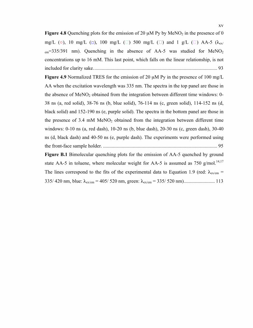
xv Figure 4.8 Quenching plots for the emission of 20 µM Py by MeNO2 in the presence of 0

mg/L (○), 10 mg/L (□), 100 mg/L (�) 500 mg/L (�) and 1 g/L (�) AA-5 (λex/

em=335/391 nm). Quenching in the absence of AA-5 was studied for MeNO2

concentrations up to 16 mM. This last point, which falls on the linear relationship, is not

included for clarity sake. ................................................................................................... 93

Figure 4.9 Normalized TRES for the emission of 20 µM Py in the presence of 100 mg/L

AA when the excitation wavelength was 335 nm. The spectra in the top panel are those in

the absence of MeNO2 obtained from the integration between different time windows: 0-

38 ns (a, red solid), 38-76 ns (b, blue solid), 76-114 ns (c, green solid), 114-152 ns (d,

black solid) and 152-190 ns (e, purple solid). The spectra in the bottom panel are those in

the presence of 3.4 mM MeNO2 obtained from the integration between different time

windows: 0-10 ns (a, red dash), 10-20 ns (b, blue dash), 20-30 ns (c, green dash), 30-40

ns (d, black dash) and 40-50 ns (e, purple dash). The experiments were performed using

the front-face sample holder. ............................................................................................ 95

Figure B.1 Bimolecular quenching plots for the emission of AA-5 quenched by ground

state AA-5 in toluene, where molecular weight for AA-5 is assumed as 750 g/mol.14,17

The lines correspond to the fits of the experimental data to Equation 1.9 (red: λex/em =

335/ 420 nm, blue: λex/em = 405/ 520 nm, green: λex/em = 335/ 520 nm). ........................ 113

xvi

List of Schemes

Scheme 1.1 Separation of crude oil into saturates, aromatics, resins and asphaltenes

based on their solubility (adapted from reference 7). ......................................................... 3

Scheme 1.2 (a) Hypothetical continental model for an asphaltene molecule and (b) a

cartoon representation of asphaltene stacks. The aggregation number and the relative

positioning of the monomers are arbitrary (adapted from reference 12). ........................... 7

Scheme 1.3 (a) Hypothetical archipelago model for an asphaltene molecule and a cartoon

representation of (b) asphaltene linear “oligomer”, (c) asphaltene branched “oligomer”,

where the active sites of asphaltene molecules are present as open circles, and (d)

asphaltene “micelles” as described by Sheu. The aggregation number and the relative

positioning of the monomers are arbitrary (adapted from reference 23 and 33). ............... 8

Scheme 1.4 Jablonski diagram. Radiative transitions are depicted with straight arrows,

and non-radiative transitions are depicted with curly arrows. E, S0, S1 and T1 represent

energy, the ground state, singlet excited state and triplet excited state, respectively. ...... 12

Scheme 1.5 Competitive deactivation pathways for S1. .................................................. 13

Scheme 1.6 Deactivation of S1 by quenching. ................................................................ 17

Scheme 1.7 Complexation of S0 and Q. .......................................................................... 18

Scheme 1.8 Structure of pyrene. ...................................................................................... 20

Scheme 3.1 Intra-aggregates quenching and bimolecular quenching (Shaded stars:

excited chromophores, open ellipse: quenchers, and open stars: unexcited

chromophores). …………………………………………………………………………72

xvii

List of Abbreviations

A absorbance

AA-5 50% heptane-insoluble Athabasca asphaltene

Ai pre-exponential factor for species, i

Ant anthracene

Å angstrom

ca. approximately

cm centimetre

CMC critical micelle concentration

CNAC critical nanoaggregate concentration oC degree Celsius

E energy

F fluorescence

g gram

h Plank’s constant (6.63 x 10-34 J·s)

HPLC high performance liquid chromatography

I intensity

I0 initial intensity

IC internal conversion

IRF instrument response function

ISC intersystem crossing

k0 intrinsic decay rate constant

kf fluorescence rate constant

kIC internal conversion rate constant

kISC intersystem crossing rate constant

kobs observed rate constant

kq quenching rate constant

Keq equilibrium constant

L litre

λ wavelength (nm)

xviii λem emission wavelength

λex excitation wavelength

M molar

MeNO2 nitromethane

mg milligram

mL millilitre

mm millimetre

mM millimolar

mol mole

µL microlitre

µm micrometre

µM micromolar

µs microsecond

N nitrogen

Ni nickel

nm nanometre

ns nanosecond

O oxygen

P phosphorescence

PAH polyaromatic hydrocarbon

PRODEN 6-propionyl-2-(N,N-dimethylamino) naphthalene

Py pyrene

Q quencher

Φf fluorescence quantum yield

s second

S sulphur

S0 ground state

S1 singlet excited state

SPC single photon counting

t time

T1 triplet excited state

xix TRES time resolved emission spectra

<τ > average lifetime

τ0 fluorescence lifetime

τobs, τi observed lifetime (of component, i)

V vanadium

Vis-NIR visible-near infrared

VR vibrational relaxation

v frequency (s-1)

UV ultraviolet

UV-Vis ultraviolet-visible

xx

Acknowledgments

I would like to thank my supervisor, Dr. Cornelia Bohne, for her encouraging

guidance and assistance throughout my graduate study time.

Special thanks to Luis Netter, for all the technical support; Hao Tang, who gave

me great help when I started the work in the lab and the latter work throughout these

three years; Tamara Pace, Rui Li and Cerize Santos, for their great professional help. I

would also like to thank many colleagues in Bohne’s research group and in the chemistry

department.

Finally, I would like to thank COSI for the funding and provide the study

opportunities.

xxi

Dedication

To my dear family

1. INTRODUCTION

1.1 Asphaltenes

1.1.1 The importance of asphaltenes

Asphaltenes correspond to the heaviest portion of crude oil, and solubility

properties are used to separate them from the lighter portions of crude oils. Asphaltenes

have applications as construction materials, such as for road pavement, and for roofing.

Other lighter fractions of crude oils, such as butanes, gasoline, naphtha, and kerosene, are

used as fuels or as industrial materials. These lighter fractions have higher commercial

value as compare to asphaltenes.1

Crude oil has been used as an energy source for over one hundred years and it

accounts for a large percentage of the energy consumption around the world. Crude oil

can be classified into two categories: conventional oil and unconventional oil.2 The oil

extracted using methods for traditional oil well extraction is normally classified as

conventional oil. On the other hand, unconventional oil refers to crude oil extracted using

techniques other than oil well methods. Conventional oil is generally less dense and easy

to refine compare to unconventional oil. Unconventional oil contains heavy oil, extra

heavy oil and oil sands.3 Unconventional oils are very viscous and some of them are

solids, and for this reason they cannot be processed using traditional extraction and

refining methods. Alternative methods have to be established in order to process

unconventional oil, which increases the cost and lowers the economic value of these oil

sources. Thus, conventional oil used to be the predominant oil source in the oil industry.

However, the total world oil reserves include 30% of conventional oil and 70% of other

2 heavier oil sources.3 As the demand for crude oil has risen continuously, conventional oil

sources are declining, and for this reason the focus has moved to find substitution

resources for oil production, such as extracting oil from oil sands.

Oil sands are sands coated with dense and sticky oil.4 Canada has large reserves of

oil sands, and oil sands production has grown in recent years. The crude oil produced

from oil sands contributed to one-half of the Canadian oil production in 2009.5 Oil sands

contain large amounts of asphaltenes. For example, Athabasca crude oil, which comes

from one of the largest deposits of oil sands in Canada, contains about 16.9% per weight

of asphaltenes.6 Research on asphaltenes is of interest to the oil industry because

asphaltenes negatively impact oil production. For example, asphaltenes form precipitates

that clog pipelines and surface facilities. Asphaltenes also contain a significant amount of

contaminants that decrease the efficiency of oil refining, by for example poisoning

catalysts used in hydrogenation processes. Therefore, the evaluation of the properties of

asphaltenes and the understanding of the mechanism for asphaltene aggregation are very

important to make the production of oil more effective from the economical and

environmental points of view.7

1.1.2 Definition and composition of asphaltenes

The operational definition of asphaltenes is based on the solubility of the material

in defined solvents.7-9 In the laboratory, asphaltenes are precipitated from crude oil by

adding n-alkanes. The light components of crude oil soluble in n-alkane are called

maltenes. Maltenes can be further fractionated into saturated hydrocarbons, aromatic

hydrocarbons, and resins based on their solubility in defined solvents. Asphaltenes are

3 insoluble in n-alkane but soluble in toluene. The separation of asphaltenes from crude oil

is summarized in Scheme 1.1.

Scheme 1.1 Separation of crude oil into saturates, aromatics, resins and asphaltenes based on their solubility (adapted from reference 7).

The chemical composition is relatively easy to be determined in the light fractions

of crude oils. For example, butane is one of the saturated compounds in maltenes, and it

is easily distilled from crude oil because of its low boiling point (-0.5 oC).1 The boiling

points of the components of oil increase as the sizes of the molecules in the oil become

larger and the molecular weights increase. For example, most hydrocarbons found in

gasoline contain 4-12 carbons, and they have boiling points between 40-220 oC.10

Compounds in asphaltenes have big molecular sizes containing up to 30 carbon atoms,

and they usually have boiling points higher than 500 oC,11 which leave asphaltenes as

residues in the commercial distillation of crude oil.

4 Since asphaltenes are defined by their solubility and correspond to a class of

molecules with similar solubility in a defined solvent, asphaltenes are not composed of

one kind of compound but different kinds of compounds. Asphaltenes contain mainly

polyaromatic hydrocarbons (PAHs) with pendant and branched alkyl chains. Asphaltenes

are enriched in heteroatoms, such as N, O, and S, which can be part of the aromatic or

aliphatic moieties. These heteroatoms introduce polarities into the asphaltene

framework,7 by for example inducing charge separation in the fused ring systems.12 In

addition, asphaltenes contain metals, such as V and Ni. These metals form complexes

with porphyrins, which are responsible for poisoning the catalysis processes during the

upgrading of crude oil.11,13 The identification of the molecular components in asphaltenes

is complex8,11,14 and is still poorly understood.

The understanding of the molecular structure of asphaltenes has changed over

time based on the results from different experimental techniques and the development of

different theories. There are two parameters that are important to define the structures of

asphaltene molecules, one is the molecular weight, and the other one is the size of the

fused ring systems. To date, many attempts have been made to establish an average value

for the asphaltene molecular weight. Over a long period of time, from the 1930’s to

1980’s, the reported range for the molecular weight of asphaltenes was very broad. The

molecular weight was reported to be as high as 300,000 g/mol based on

ultracentrifugation experiments.15 At the same time, lower values (600-6,000 g/mol) were

also reported using different techniques, such as cryoscopic methods, viscosity

determinations, light adsorption coefficients measurements, pressure osmometry

experiments and by using the isotonic vapor pressure method.15 As a result of the high

5 molecular weight determination the structure of asphaltene was proposed to have large

aromatic systems with up to 70 aromatic rings containing heteroatoms (S, O, and N).11

The broad range of molecular weights and unrealistic big aromatic ring systems are

controversial for a single asphaltene molecule. In the past two decades, the molecular

weight of asphaltenes has been narrowed down to a range of 500-1,000 g/mol by using

advanced techniques, such as mass spectrometry16 and fluorescence spectroscopy.14,17-19

A consensus value for the average molecule weight is 750 g/mol. Also, a small

distribution (4-10) of fused rings have been reported using scanning tunnelling

microscopy,20 transmission electron microscopy,21 and molecular simulations.19,22

1.1.3 Asphaltene aggregates

Asphaltenes are known to self-associate in solution to form aggregates, which

upon further aggregation form precipitates. The self-association behaviour is attributed

primarily to π−π stacking interactions involving fused aromatic rings. In addition, acid-

base interactions and hydrogen bonding are also proposed to be important in the

aggregation of asphaltene molecules.23

One attempt to rationalize the mechanism of asphaltene aggregation is to relate it

to well-known concepts of aggregation, such as micellization.24 The concept of micelles

is widely used to describe asphaltene aggregates. However, the conventional definition

for micelles is an aggregate of surfactant molecules in solution.25 Surfactant molecules

have defined structures that contain a hydrophilic region and a hydrophobic region. In

aqueous solution, the hydrophobic effect is the driving force for the formation of

micelles. Conventional micelles are formed spontaneously from monomers as the critical

6 micelle concentration (CMC) is reached. However compared to surfactants, asphaltene

molecules are polydisperse and the mechanism of asphaltene aggregation is likely to be

more complex than for the formation of micelles. Therefore, in the description below I

am using the term “micelle” in quotation marks for literature reports that employed this

concept in order to differentiate asphaltene aggregates from conventional micelles.

Currently, there are three major models to describe the association of asphaltene

molecules.23,24,26 These models are based on different model structures for asphaltene

monomers. One model is the “Yen model”, in which different stages of aggregation in

asphaltenes were proposed.26 The Yen model is constructed based on asphaltene

monomers that contain large fused aromatic rings with short alkyl chains on the periphery

(Scheme 1.2a). This molecular structure is frequently referred to as the continental

model.27 The large planar rings are unit sheets that are proposed to stack via π−π

interactions. The results from X-ray diffraction studies supported the concept of

condensed aromatic sheets, and these sheets tend to stack together.28,29 The asphaltene

stacks were called particles in Yen’s model and he proposed that two or more particles

can cluster further to form “micelles”.26 Recently, Mullins proposed a “modified Yen

model”,12 in which the term nanoaggregates was used for the smallest unit of asphaltene

aggregates. Mullins proposed that the condensed aromatic rings stack in the interior of

the aggregates and the alkane chains reside on the exterior (Scheme 1.2b). The attractive

force between these aromatic rings makes asphaltene monomers associate with each

other, while the repulsive force between the peripheral alkane chains caused by steric

hindrance limits the size of the nanoaggregates. Thus, asphaltene monomers form

nanoaggregates with a small aggregation numbers of around 6, where the additional

7 asphaltene monomers are not able to stack onto the aromatic rings in the nanoaggregate.

Mullins defined that the asphaltene “critical nanoaggregate concentration” (CNAC) as a

concentration at which the nanoaggregates stop to growth. Mullins also proposed that the

asphaltene nanoaggregates could form “clusters”.

Scheme 1.2 (a) Hypothetical continental model for an asphaltene molecule and (b) a cartoon representation of asphaltene stacks. The aggregation number and the relative positioning of the monomers are arbitrary (adapted from reference 12).

A different molecular structure for asphaltenes, frequently refers to as archipelago

model, was proposed by Strausz,30,31 where the aromatic rings are dispersed but are

linked by side chains within the asphaltene molecule (Scheme 1.3a). Yarranton proposed

a model where specific interactions of active sites in the asphaltene molecule are

responsible for the aggregation. These interactions could be π−π stacking, acid-base

interactions, hydrogen bonding, and van der Walls interactions.32,33 Some large

asphaltene molecules contain multiple sites and act as propagators in an oligomerization-

like reaction, while other small asphaltene molecules have a single site that link with the

propagators and therefore terminate the oligomerization.6,23,32 Asphaltenes can form

linear aggregates (Scheme 1.3b), or branched aggregates (Scheme 1.3c).23 A recent study

8 on asphaltene aggregation using single molecule force spectroscopy indicated that

asphaltene aggregates appear as worm-like chain structures.33 Finally, Sheu proposed

another model of asphaltene aggregates based on the archipelago structure. In this model

the asphaltene monomers form spherical aggregates as “micelles” (Scheme 1.3d).24 It is

clear that the “micelles” from Yen’s model is different from the “micelles” proposed by

Sheu. In Sheu’s model, “micelles” refers to the smallest unit of asphaltene aggregates, but

“micelles” corresponds to the cluster of asphaltene aggregates in Yen’s paper.

Scheme 1.3 (a) Hypothetical archipelago model for an asphaltene molecule and a cartoon representation of (b) asphaltene linear “oligomer”, (c) asphaltene branched “oligomer”, where the active sites of asphaltene molecules are present as open circles, and (d) asphaltene “micelles” as described by Sheu. The aggregation number and the relative positioning of the monomers are arbitrary (adapted from reference 23 and 33).

9 As mention above, the term of “micelle” is defined differently based on different

theories. In some studies of asphaltene the concept of “micelles” is employed where the

description of their properties is the same as for conventional micelles. For example, the

measurement of surface tension, a traditional method for CMC determination in aqueous

solutions, was employed to determine the “CMC” for asphaltene.34,35 However, some

studies use “micelles” to describe a phenomenon where the presence of asphaltene

aggregates is supported by their experimental evidences. For example, the size of

“micelles” of 10-30 µm in diameter was suggested using the electron micrograph

technique and this size corresponded to a “micelle” with a weight of 37,000-10,000,000

g/mol.26 In such case, the size and the weight of these “micelles” is much larger than the

sum of several (up to 1000) asphaltene monomers. This reported “micelles” is more in

line with the size of clusters. As the term of “micelles” has been used indiscriminately

from different perspectives, the “CMC” of asphaltenes have been reported over a broad

range of concentrations (mg/L-g/L) and the differences between these values is probably

due to the different detection techniques and/or different measurable physical parameters

measured. In recent studies the term “nanoaggregates” have been used to avoid the

confusion around the use of “micelles”. The asphaltene CNAC have been reported to be

in the range of mg/L by using different techniques, such as centrifugation,36 high-Q

ultrasonics,37 electrical conductivity measurements,38 gas chromatography,39 mass

spectroscopy,39 NMR diffusion measurement,40 and fluorescence measurements.41,42

The aggregation behaviour of asphaltenes depends on the solvent that is used to

solubilize it. For example, some studies of asphaltene aggregation are performed in

toluene, while other studies are carried out in crude oil. In toluene, asphaltene molecules

10 are believed to be dispersed as a true solution at very low concentrations (ca. ~0.2-2

mg/L).43 Previous work reported the formation of asphaltene aggregates at concentrations

as low as 50-80 mg/L in toluene.17,44-46 In crude oil, asphaltene molecules are believed to

start to aggregate at higher concentrations than in toluene because of the presence of

resins, which can stabilize the asphaltenes in solution.6,11 Resins have similar structures to

asphaltenes but they have lower molecular weights and a smaller fraction of aromatic

carbons.11,32 Resins dissolve in alkanes because they contain alkane chains and they are

relatively small in size. Resins also contain aromatic rings that can have π−π interactions

with asphaltene molecules. Thus, resins can be adsorbed on the surface of asphaltenes

and stabilize asphaltenes in solution.11

1.1.4 Fluorescence of asphaltenes

Asphaltenes are colored solids, either brown or black depending on the separation

method employed. Many of the asphaltene components are fluorescent and they are

photochemically stable under near-visible and visible light.47 Therefore, photophysical

properties, such as fluorescence, can be used to study asphaltenes. Compared to other

techniques, fluorescence is a very sensitive technique to detect analytes at very low

concentrations, even at a single molecule level.48 The fluorescence properties of many

molecules are sensitive to the molecules’ surrounding environment.25,49,50 Therefore, it is

possible to use fluorescent probes to fingerprint the various environments present in

microheterogeneous media.25 The background information about fluorescence and related

photophysical techniques will be introduced next before the discussion of the previous

fluorescence studies on asphaltenes.

11 1.2 Photophysical techniques

1.2.1 Unimolecular photophysical processes

Photophysical processes are processes related to a molecule gaining energy by

absorbing a photon, or losing energy by releasing heat or emitting a photon. The

transitions between energy levels are divided into two categories: the processes that

involve the absorption or emission of photons are called radiative transitions, while the

processes that involve the release of heat in the deactivation of the excited state molecule

are non-radiative transitions. In particular, absorption (A), fluorescence (F) and

phosphorescence (P) are the possible radiative transitions. Internal conversion (IC),

intersystem crossing (ISC) and vibrational relaxation (VR) are the possible non-radiative

transitions. The various photophysical processes are summarized in the Jablonski

diagram and are represented in Scheme 1.4.

12

Scheme 1.4 Jablonski diagram. Radiative transitions are depicted with straight arrows, and non-radiative transitions are depicted with curly arrows. E, S0, S1 and T1 represent energy, the ground state, singlet excited state and triplet excited state, respectively.

Absorption (A) is a phenomenon where the energy of an electromagnetic

radiation is absorbed by a molecule. During this process, the molecule is excited from the

ground state to one of its electronic excited states. The excited state molecule is unstable

and will return to its ground state through various deactivation pathways. IC is the non-

radiative transition between electronic states with the same spin state, while ISC is the

non-radiative transition between electronic states with different spin states. Fluorescence

(F) is the radiative transition between electronic states with the same spin multiplicity (S1

→ S0 + hv), while phosphorescence (P) is the radiative transition between electronic

states with the different spin multiplicity (T1 → S0 + hv). VR is a rapid transition (<10-12

s)48 between vibrational levels in the same electronic state in solution phase, and the

13 fluorescence and phosphorescence are always from the lowest vibrational energy level of

the excited state to the ground states.

In this thesis, the fluorescence properties of asphaltenes were investigated, and for

this reason the deactivation processes from the triplet excited states (T1) are not

discussed. Fluorescence (F), IC, and ISC are competitive intramolecular photophysical

processes for the deactivation of S1. These deactivation processes correspond to first-

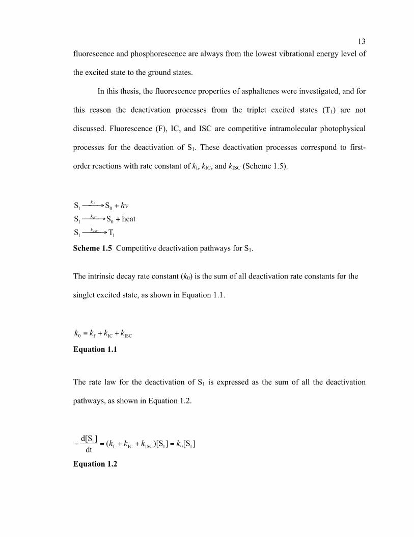
order reactions with rate constant of kf, kIC, and kISC (Scheme 1.5).

11

01

01

TS

heatSS

SS

!!→!

+!→!

+!→!

ISC

IC

f

k

k

k hv

Scheme 1.5 Competitive deactivation pathways for S1.

The intrinsic decay rate constant (k0) is the sum of all deactivation rate constants for the

singlet excited state, as shown in Equation 1.1.

ISCICf0 kkkk ++=

Equation 1.1

The rate law for the deactivation of S1 is expressed as the sum of all the deactivation

pathways, as shown in Equation 1.2.

]S[]S)[(dt]d[S

101ISCICf1 kkkk =++=−

Equation 1.2

14 The concentration of the singlet excited state molecule [S1] at time t is expressed as a

mono-exponential function (Equation 1.3),

t011

0e][S][S k−=

Equation 1.3

where [S1]0 is the initial concentration of the singlet excited state molecule (S1).

The fluorescence lifetime of a molecule (τ0) is defined as the amount of time it

takes for the concentration of the singlet excited state molecule to decrease to 1/e of the

initial value. Therefore, the fluorescence lifetime is expressed as the inverse of the

intrinsic decay rate constant, as shown in Equation 1.4.

€

τ0 =1k0

Equation 1.4

Typical timescales for fluorescence lifetimes are of the order of 10-12 to 10-8 s.51

The fluorescence quantum yield (Φf), is given by the number of photons emitted as

fluorescence relative to the total number of photons absorbed by the molecule (Equation

1.5).

0f0

ff τkkk

==Φ

Equation 1.5

15 1.2.2 Steady-state fluorescence emission spectra

The steady-state fluorescence emission spectrum corresponds to the distribution

of emission intensities as a function of wavelength. Experimentally, the emission

spectrum is obtained by exciting a sample with a continuous irradiation at a certain

wavelength and monitoring the intensity at various emission wavelengths.

1.2.3 Time-resolved fluorescence decay measurements: single photon counting

Fluorescence lifetimes are measured using a single photon counting (SPC)

technique. In this technique, the fluorescence emission intensity is measured as a function

of time. Experimentally, a pulsed light source excites the sample and causes the sample to

emit photons. The time for the first photon detected after the excitation pulse is measured.

For each photon detected a count is stored in an array that contains 1,000 channels, which

correspond to incrementally longer time intervals. The distribution of counts stored in the

1,000 channels after repeating the pulsed experiment many times represents the time

dependence of the fluorescence emission, which is a fluorescence decay profile.48

When one type of fluorophore with a single fluorescence lifetime is present in the

sample, the fluorescence decays correspond to a mono-exponential decay and fit to

Equation 1.3, where the concentration of singlet excited state molecules is proportional to

the fluorescence intensity. When the sample contains more than one fluorophore with

different lifetimes, the decay follows a sum of exponentials (Equation 1.6),

16 )t(i

1i

ie)t( τ−

∑= AI

Equation 1.6

where I(t) is the emission intensity or the number of counts, and τi is the lifetime of the

emitting species, i and t is time. Ai is the pre-exponential factor of the emitting species, i,

with the sum of all pre-exponential factors normalized to unity. The pre-exponential

factor of each emitting species corresponds to the abundance of that component in the

total emission.

1.2.4 Time-resolved emission spectra

Time-resolved emission spectra (TRES) are the emission spectra collected at

specific time windows after the excitation pulse. The steady-state fluorescence emission

spectra are related to all chromophores in solution, while TRES are related the species

that emit within a particular time window. Experimentally, fluorescence decays are

collected at different emission wavelengths for the same amount of time. TRES are

constructed by integrating the decay intensities for each emission wavelength between

defined delays windows after the excitation pulse. At short delays long lived and short

lived species contribute to the TRES, while at long delays after excitation the short lived

species have decayed and only the spectrum for the long lived species is measured.

17 1.2.5 Bimolecular photophysical processes

The intramolecular deactivation pathways of the excited states discussed so far

are unimolecular processes. The intermolecular deactivation of the excited state

molecules by another molecule (the same molecule or different molecule) is a

bimolecular process, called quenching,48 as shown in Scheme 1.6,

QSQS 01q +!→!+ k

Scheme 1.6 Deactivation of S1 by quenching.

where quencher (Q) refers to a substance that can accelerate the deactivation of the

excited state molecule and kq is the quenching rate constant. The overall rate law for the

deactivation of S1 is expressed as the sum of the rate of the unimolecular and bimolecular

processes, as shown in Equation 1.7.

][Q][S]S[dt]d[S

1q101 kk +=−

Equation 1.7

Quenching studies are usually carried out as pseudo first order reactions, where

the quencher concentration is in excess over the S1 concentration. Therefore, [Q] is

considered as a constant and Equation 1.7 can be integrated as Equation 1.8,

t])Q[(011

q0e][S][S kk +−=

Equation 1.8

18 where the decay of S1 follows a first-order function. The observed rate constant (kobs) and

the observed fluorescence lifetime (τobs) are expressed in Equation 1.9:

]Q[1q0obs

obs

kkk +==τ

Equation 1.9

Quenching can be static or dynamic. Static quenching takes place if there is the

formation of nonfluorescent complexes (S0Q) between the ground state molecules (S0)

and quenchers (Q) with equilibrium constant Keq (Scheme 1.7).

Scheme 1.7 Complexation of S0 and Q.

The complexes S0Q normally absorb light, but the quenching in the complex is

immediate and no fluorescence occurs. An increase in the quencher concentration leads

to a decrease of the concentration of the excited state molecules S1 formed because a

larger amount of the ground state is tied up in the non-fluorescent complex S0Q.

Therefore, static quenching decreases the emission intensity of S1, while static quenching

has no influence on fluorescence lifetime of S1,48 as shown in Equation 1.10 and 1.11:

]Q[1 eq0 KII

+=

Equation 1.10

19

1obs

0 =ττ

Equation 1.11

Dynamic quenching is also called collisional quenching. The collision happens

between a quencher molecule and the singlet excited state (S1) to form an encounter

complex, where quenching occurs. The static quenching does not rely on diffusion or

molecular collisions, but dynamic quenching does.48 Static and dynamic quenching both

decrease the concentration of excited state molecules (S1), so they lower the emission

intensity. However, dynamic quenching shortens the fluorescence lifetime and the

fluorescence intensity at the same time48 because quenching is an additional deactivation

process for the excited states. The ratio of the fluorescence lifetimes and intensities in the

absence and presence of the quencher is given by Equation 1.12 in the case of dynamic

quenching.

][1 0q0

obs

0 QkII

τττ

+==

Equation 1.12

1.3 Pyrene

Externally added probe, such as Pyrene (Py, Scheme 1.8), might interact with a

subset of the components of asphaltene. The quenching experiments of probes in the

presence of asphaltene aggregates by quenchers will determine if the probes are located

inside the aggregates or free in the solution. Probes in the interior of the aggregates are

20 expected to have lower quenching rate constants than probes that are exposed in the

solution.

Py is a common probe used in fluorescence studies of organized systems.25,49 The

dimensions of Py are 10.4 Å long and 8.2 Å wide.52 Its size is relatively small compared

to the size of asphaltene aggregates.

Scheme 1.8 Structure of pyrene.

Py is a very popular fluorescent probe because it has a very long fluorescence

lifetime (190 ns in non-polar solvent and 650 ns in polar solvent)53 and a high

fluorescence quantum yield (0.65 in non-polar solvent and 0.72 in polar solvent).53 More

importantly, the fluorescence spectrum and fluorescence lifetime of Py are very sensitive

to the surroundings of the excited state Py. 49,54-57

Py has limited solubility (1.6 x 10-6 M) in water.58 Its solubility in water can be

enhanced when Py is incorporated into a hydrophobic cavity of a host system. For this

reason Py was used as probe on study several organized systems in the aqueous

solutions.25,49,54 Also, Py can be employed to study aromatic systems in the organic

phase,59 since Py has a conjugated aromatic system and it can bind with other aromatic

systems via π−π interactions. For this reason, Py was employed as probes to study the

polydisperisty of aggregates present in asphaltene solutions.

21 1.4 Review of the fluorescence studies with asphaltenes

Fluorescence has been employed to study crude oils and asphaltenes, either by

exploring the intrinsic emission spectra,17,19,41-45,47,60-67 or by measuring the fluorescence

lifetimes.46,47,62,63,68-70 The emission spectra41,42,44,45,47,65 and lifetimes46,47,62 for

asphaltenes and oil samples are dependent on the concentration of the samples.

The studies involving the measurement of steady-state fluorescence emission

spectra showed that the intensity of the emission decreased when the concentration of

asphaltenes or oil samples were increased. Some authors interpreted that the intensity

decreases were due to quenching inside the asphaltene aggregates.42,45,65 Other authors

rationalized that these decreases were due to the high optic density of the solutions.41 In

addition, red shifts of the emission spectra for asphaltenes were observed with the

increase in the concentration of the samples, which was also attributed to

aggregation.41,42,45

The CMC or CNAC determined from the steady-state fluorescence experiments

have been reported over a broad concentration range from 50 mg/L to 1.6

g/L.41,42,44,45,47,65 The differences in these values are due to different experimental

conditions, such as the solvent, the excitation wavelengths and the way the fluorescence

measurement are carried out for the concentrated solutions. The solvent dependence of

the CMC or CNAC values is reasonable since asphaltene is defined as a solubility class.

The wavelength dependence on the asphaltene aggregation behaviour can be rationalized

by the fact that the chromophores with different excited state energies may start to

aggregate at different concentrations. The red shift observed at high asphaltene

concentrations could be related to self-absorption, which is an artifact that will be

discussed in the Experimental section (2.3.5). Front-face detection41,65 or short light

22 pathlength42,45 were employed to solve the self-absorption problem. However, no

systematic procedure has been established to test how well the self-absorption was

diminished.

Time-resolved fluorescence experiments have been used recently to investigate

the lifetimes for the intrinsic emission of crude oils and asphaltenes.46,47,62,63,68,70 Wang et

al. found that an increase of the fluorescence lifetimes for oil samples was observed with

an increase in the dilution of the crude oil.47 Ryder et al. studied the fluorescence

lifetimes for oil samples that contain a known content of aromatic compounds. The

results showed that the fluorescence lifetimes were increased as the concentration of

aromatic compounds in oils decreased.63,70 Both results suggest that high concentrations

of chromophores lead to efficient collisional quenching and energy transfer in the oil

samples. Similarly, the fluorescence lifetimes of asphaltenes also showed a dependence

on the concentration,46,62 in which the lifetimes decrease as the concentrations of

asphaltenes increase. This observation suggests the formation of aggregates.

Some experiments were carried out at different excitation and/or emission

wavelengths. At a fixed excitation wavelength, the lifetimes for the emission of crude oils

increased as the emission wavelength became longer.47 Ryder et al. confirmed these

observations; however, he noticed that this increase occurred for a certain wavelength

range. A maximum lifetime was obtained between 600 and 700 nm for various oil

samples, and the lifetimes decreased for emission wavelengths longer than 700 nm.63,70

This observation was assigned to the interplay between collisional energy transfer and

quenching processes.

23 Beside the possible quenching between the chromophores in the asphaltene

solution, the quenching of the fluorescence of asphaltenes by an externally added

quencher, such as o- and p-chloranil, was observed.69 In this experiment, the lifetimes for

the excited state of asphaltenes remained the same with the addition of quencher,

indicating that a static quenching mechanism involving ground-state complexation of

asphaltene with the quencher occurs.

As mentioned earlier in section 1.1.4, externally added probes can be employed to

characterize the various environments present in microheterogeneous media. The use of

6-propionyl-2-(N,N-dimethylamino) naphthalene (PRODEN) as an external probe

showed a slightly red shift of its emission with the addition of asphaltenes.41 The authors

concluded that the probe was incorporated into a polarizable site in the asphaltene

aggregates. On the other hand, fluorescence lifetimes of probe molecules were measured

with the addition of crude oils.71 It was found that a significant quenching of the lifetime

for the excited state probes occurred by the aromatic moieties present in crude oil.

Analysis of these results indicates that the observed lifetime decay rate constant is

linearly correlated to the concentration of crude oil.

1.5 Thesis objectives

Asphaltenes are usually considered a problem because they form aggregates

easily and further form precipitates that clog the pipelines and surface facilities in the oil

industry. Thus, asphaltenes aggregation is an active area of research.12,14,33,36,37,42,45,72,73

The intrinsic fluorescence properties of asphaltenes have been studied, but the

mechanism of asphaltene aggregation is still poorly understood. Probe molecules have

24 been previously employed to study the asphaltene aggregation, but no successful

characterization of the asphaltene aggregates has yet been achieved.

The primary objective of this work was to establish appropriate methodologies to

be used for the characterization of the intrinsic fluorescence of asphaltenes by measuring

steady-state emission spectra, time-resolved fluorescence decays and time-resolved

emission spectra. The combination of the use of complementary fluorescence techniques

was employed to study the aggregation of asphaltenes by exploring the intrinsic emission

from asphaltene solutions at different concentrations.

The second objective of this work was to quench the intrinsic asphaltene emission

to determine the accessibility of quenchers to the asphaltene aggregates. This work can be

used to determine how accessible the interior of the asphaltene aggregate is to small

molecules, and also determine if the accessibility of the small molecule is different for

the aggregates formed from different asphaltene components.

The third objective of this thesis was to quench externally added probes that might

be incorporated in asphaltene aggregates. The probe molecule employed was Py, because

it has a long fluorescence lifetime that can be well distinguish from the asphaltene

lifetime. Also, Py has a high fluorescence quantum yield and for this reason only a low

concentration is required to give sensitive fluorescence measurements. In addition, Py

was employed as a fluorescent probe to study the aggregation of asphaltenes because Py

might interact with a subset of the components of asphaltenes through π−π stacking. If

the π−π interactions between the Py and the subset of the aromatic components of

asphaltene exist, Py should have a different fluorescence lifetime in the aggregates. A

lower quenching efficiency would be expected for the Py inside the asphaltene aggregates

25 when they are less accessible to the quencher molecules. In this respect, the information

obtained from the quenching experiments using externally added Py would complement

the studies from the intrinsic asphaltene fluorescence, in which the the ability of small

molecules to enter the particular binding sites that form through π−π interactions would

be investigated.

26

2. EXPERIMENTAL

Some of the results presented in this chapter have been published in the Photochemical &

Photobiological Sciences. Reproduced by permission of The Royal Society of Chemistry

(RSC) on behalf of the European Society for Photobiology, the European Photochemistry

Association, and RSC. This open access article can be accessed via the website (at

http://pubs.rsc.org/en/content/articlelanding/2014/pp/c4pp00069b).

2.1 Materials

Athabasca asphaltene (AA-5, 50% heptane-insoluble asphaltene, obtained from

Dr. Murray Gray’s group, University of Alberta),74 nitromethane (MeNO2, 99+%,

Aldrich), anthracene (Ant, 99+%, Aldrich), and toluene (Caledon, spectroscopic grade)

were used as received. Pyrene (Py, 99%, Aldrich) was recrystalized once from 95%

ethanol. The purity of Py was checked using single photon counting (SPC) experiments

to measure the fluorescence decay of Py in aerated aqueous solutions. For pure Py a

mono-exponential decay (τ = ~130 ns) was obtained,54 while impure samples showed a

fast decay in addition of the long decay due to the Py emission.

2.2 Sample preparations

Stock solutions of AA-5 (1 g/L or 10 g/L) were prepared by dissolving

appropriate amounts of the AA-5 solid in toluene. A series of dilutions (0.1 mg/L to 5

g/L) were prepared by adding the stock solution into toluene using an Eppendorf®

pipette. A stock solution of Py (2-5 mM) was prepared by dissolving appropriate amounts

of Py solid in toluene. Py samples (20 µM) were prepared by injecting appropriate

amounts of the Py stock solution into toluene or AA-5/toluene solutions. A stock solution

27 of Ant (1.35 mM) was prepared by dissolving appropriate amounts of Ant solid in

toluene. Ant samples (20 µM) were prepared by injecting the Ant stock solution into

toluene.

MeNO2 was used as a quencher and its stock solutions (~1 M) were prepared

daily by injecting appropriate volumes of neat MeNO2 into toluene. Appropriate volumes

of the quencher stock solution were added to 2.5 mL of AA-5 or Py solutions using a

Hamilton gastight glass syringe.

All samples were contained in 10 x 10 mm quartz cells. Oxygen is an efficient

quencher of singlet excited states,75 and Py has a long excited state lifetime. For these

reasons, all Py samples used for SPC experiments and the quencher solutions used for the

quenching of excited state Py were deaerated. Samples were bubbled with nitrogen for at

least 30 min. The Ant samples used for SPC experiments were aerated solutions, since

Ant has a short excited state lifetime (ca. ~4 ns) in toluene.

Oxygen quenches the lifetime of the excited states in AA-5 samples. In

preliminary studies, the SPC experiments for AA-5 samples were performed under

different conditions: (i) aerated solutions, (ii) deaerated solutions by bubbling nitrogen

for at least 30 min and (iii) oxygen saturated solutions by bubbling oxygen for at least 30

min. Unless otherwise stated, lifetimes measurements for AA-5 samples at different

concentrations and quenching experiments for the excited states of AA-5 were done with

aerated solutions.

Two or more independent experiments were performed to check the

reproducibility of data (refer to section 3.2.2.1). Independent experiments for AA-5

lifetime measurements means that the experiments were done with solutions prepared

28 separately by dissolving a new portion of AA-5 solid in toluene, and measuring lifetimes

on different days. Independent experiments for Py lifetime measurements means that the

experiments were done with the solutions prepared with the same or different stock

solutions of Py but deaeration of the solutions were done on different days.

2.3 Instrumentation

2.3.1 UV-Vis absorption spectroscopy

Absorption spectra were recorded with a Varian Cary 1 UV-Visible

spectrophotometer at room temperature, and the spectra were collected between 250 nm

and 600 nm. Correction of spectra was done by subtracting the absorption spectrum of

solvent (toluene) from the absorption spectrum of sample solutions.

2.3.2 Steady-state fluorescence spectroscopy

Steady-state fluorescence emission spectra were collected with a Photon

Technology International® (PTI) QuantaMasterTM (QM-2) fluorimeter. The excitation

light source was a Xenon lamp. Excitation and emission slits were set to correspond to a

bandwidth between 2 and 3 nm, depending on the sample’s fluorescence intensity. The

step size and integration time were 0.5 nm and 0.25 s, respectively. All measurements

were done at room temperature. Unless otherwise stated, corrected spectra were obtained

by subtracting the spectra for the solvent (toluene) from the spectra for the samples. This

correction procedure is required to remove the Raman scattering from the solvent.

29 2.3.3 Time-resolved fluorescence decay measurements using single photon counting

(SPC)

Time-resolved fluorescence decay measurements were performed with an

Edinburgh OB 920 SPC system. The excitation light sources were an Edinburgh EPLED-

330 light emitting diode and an Edinburgh EPL-405 laser diode, where the excitation

wavelengths were centered at 335 nm and at 405 nm, respectively. When the excitation

wavelength was 335 nm, the lifetime measurements for the emission of AA-5 samples

were collected at emission wavelengths of 391 nm, 420 nm or 520 nm. When the

excitation wavelength was 405 nm, the lifetime measurements for the emission of AA-5

samples were collected at 520 nm. The lifetime measurements for the emission of Py in

the absence or in the presence of AA-5 were done by exciting the samples at 335 nm and

by collecting the emission at 391 nm. Unless stated otherwise the detection

monochromator width was set to 2 mm which corresponds to a bandwidth of 16 nm.

Unless stated otherwise the total number of accumulation counts was 10,000 at the

channel of maximum emission intensity. The instrument response function (IRF) was

collected with an aqueous Ludox (Aldrich) solution to scatter light at the excitation

wavelength. The shapes of the IRF are as expected from the profiles for the EPLED-330

and EPL-405 supplied by Edinburgh Instrument.76,77 All the SPC measurements were

done at room temperature.

The emission decays were fit to a sum of exponentials (Equation 1.6) using the

software provided by Edinburgh. The lifetimes for the emission of AA-5 samples were

short (≤ 20 ns), the IRF was deconvoluted from the decays to obtain the fit curve. This

procedure eliminates both the noise and the effects of the exciting light pulse. In the case

30 of Py emission, its lifetime was long (ca. 305 ns) and the decay were fit using a “tail” fit

in which no deconvolution was performed, because the IRF was collected over too

narrow a window of time, i.e. it was collected in too small a number of channels. χ2 is

called the “reduced chi-square”, its values are used to scale the “goodness of fit”. In

addition, the residuals between the origninal data and the fitting curve were used to

evaluate the goodness of the fits. The fits with χ2 values between 0.9 and 1.2 and a

random distribution of residuals around 0 were considered to be acceptable.50

2.3.4 Time-resolved emission spectra (TRES)

TRES were constructed from time-resolved fluorescence decays with the same

SPC system mentioned above. The experiments were done by exciting a sample at a fixed

wavelength and collecting the decays at different emission wavelengths for the same

amount of time. TRES were constructed using the Edinburgh software by integrating the

intensities between defined time windows. TRES were usually normalized at the

wavelengths of maximum intensity in order to compare changes in the shape of the

spectra with time.

The excitation wavelength was 335 nm for AA-5 samples. Raman scattering of

toluene was detected at 360 and 380 nm as an emission with the same time profile as the

IRF. The Raman scattering emission was visible in some spectra ([AA-5] ≤ 10 mg/L).

Therefore, the emission decays for AA-5 samples were collected from 400 nm to 600 nm

at each 20 nm to construct the TRES. The excitation wavelength was 335 nm for Py

samples, where the intensity of Raman scattering emission was very low compared to the

31 emission intensity of 20 µM Py; therefore, the emission decays for Py samples were

collected from 360 nm to 450 nm at each 5 nm.

2.3.5 The usage of the front-face sample holder

The fluorescence intensity of a sample is directly related to the fluorescence

quantum yield of a particular molecule and the concentration of excited states formed in

the absorption process. In principle, a linear relationship exists between the fluorescence

intensity and the absorbance of a sample. However, depending on the geometry employed

between the excitation beam and the emission detection this relationship only holds at

low absorbance values at the excitation wavelength. Fluorescence is normally measured

at a 90 degree angle between the excitation and emission optics. In this case, at high

absorbance values the number of photons reaching the sample volume from which

emission is collected is not directly related to the concentration of fluorophore and

smaller emission intensities are observed than predicted from the absorbance values. This

decrease in intensity is proportionally the same for the whole emission spectrum.

The fluorescence of a sample is also affected by self-absorption when the

emission and absorption spectra overlap and the emission pass through the solution

before being detected. This situation occurs with the 90 degree arrangement between the

excitation source and the emission detection where the excitation normally occurs in the

centre of the cell. Self-absorption is increased with an increase in the pathlength and it is

more prominent at wavelengths where the molar absorptivity of the sample is higher.

Therefore, self-absorption leads to a distortion of the emission spectrum with a larger

decrease of the emission intensity being observed where the absorption of the sample is

32 higher. The solution to the self-absorption problem is to use a front-face illumination set-

up where the excitation and emission occur at the same surface of the solution.

Triangular cells are traditionally used for front-face measurements, but specular

reflections can lead to artifacts. A sample holder (Figure 2.1 from Edinburgh) was

employed which holds 10 x 10 mm cell in which the sample is titled backwards by 30

degrees and there is a 52 degree angle with respect to the normal for excitation beam and

emission optics.

Figure 2.1 Geometry for the front-face sample holder from Edinburgh (Diagram provided by Edinburgh Instruments Ltd.)

In this thesis, the front-face sample holder was employed to measure the

fluorescence for samples with high concentrations, and a sample holder with the common

arrangement of a 90 degree angle between the excitation beam and the detection optics

33 was employed for diluted samples. The switch of two sample holders between

concentrated and diluted samples will be illustrated in section 3.2.1.1.

34

3. INVESTIGATION OF THE ASPHALTENE AGGREGATION AND THE

ACCESSIBILITY OF QUENCHERS TO ASPHALTENE AGGREGATES

USING FLUORESCENCE STUDIES

Some of the results presented in this chapter have been published in the Photochemical &

Photobiological Sciences. Reproduced by permission of The Royal Society of Chemistry

(RSC) on behalf of the European Society for Photobiology, the European Photochemistry

Association, and RSC. This open access article can be accessed via the website (at

http://pubs.rsc.org/en/content/articlelanding/2014/pp/c4pp00069b).

3.1 Introduction

Asphaltenes are black or brown solids that absorb light in the near visible and

visible region of the spectrum. In general, the fluorescence properties of molecules, such

as their emission spectra and their singlet excited state lifetimes, are related to the

molecules’ surrounding environment.25 As the asphaltene molecules form aggregates, the

environment where the molecules are located is different from the environment when the

molecules are free in solution. The fluorescence of asphaltenes has been previously

employed with some success to investigate asphaltene aggregation.17,19,41-45,47,60-67 The

purpose of the current work was to provide a more comprehensive use of complementary

fluorescence techniques. The combination of the use of steady-state fluorescence

emission spectra, time-resolved fluorescence lifetime and time-resolved emission spectra

(TRES) measurements was employed to study the aggregation of asphaltenes by

exploring the intrinsic emission from asphaltene solutions at different concentrations.

35 Additional information can be obtained from quenching studies. Fluorescence

quenching is a bimolecular process and quenching experiments can be used to investigate

the accessibility of small molecules to fluorophores located in the asphaltene aggregates.

A lower quenching efficiency is expected when the accessibility of the quencher to the

chromophores inside the aggregates is decreased. In this work, the quenching efficiency

was obtained from time-resolved fluorescence experiments because the data from steady-

state spectra were difficult to interpret due to self-absorption of the asphaltene emission

at high asphaltene concentrations.`

3.2. Results

3.2.1 Steady-state fluorescence of AA-5 asphaltene

3.2.1.1 Self-absorption of the AA-5 asphaltene emission at high asphaltene

concentrations

The fluorescence for diluted samples was measured with a 90 degree arrangement

between the excitation source and the detection optics (see section 2.3.5). As the

concentration of asphaltene was increased, the fluorescence of samples with high

absorbance values at the excitation wavelength cannot be measured correctly using a 90

degree arrangement because of the absorption of the emitted light by the sample, i.e. self-

absorption. The front-face sample holder was employed at high fluorophore

concentrations. To use the front-face sample holder one needs to define the transition

between diluted and concentrated samples where self-absorption becomes a problem to

accurately determine the fluorescence intensity. In a control experiment, the fluorescence

spectra of a series of concentrations of AA-5 samples from 10 mg/L to 10 g/L in toluene

36 were collected using both a 90 degree arrangement between the excitation beam and the

detection optics and the front face sample holder. It was found that the fluorescence

spectra for the samples with absorbance values around 1 or higher than 1 at the excitation

wavelengths, obtained using a 90 degree arrangement for the excitation/emission optics

were red shift in comparison to the spectra obtained when using the front-face sample

holder. Two samples, 10 mg/L and 50 mg/L AA-5 in toluene were chosen to show this

effect. The absorption spectra of the two samples are shown in Figure 3.1. At 310 nm, the

absorbance was about 0.25 for the sample containing 10 mg/L AA-5 and was about 1.3

for the sample with 50 mg/L AA-5.

Figure 3.1 Absorption spectra for 10 mg/L AA-5 (a) and 50 mg/L AA-5 (b) in toluene.

The normalized fluorescence emission spectra excited at 310 nm for the two

samples are shown in Figure 3.2. A red shift was observed for the spectrum of the

solution with 50 mg/L AA-5 obtained using a 90 degree arrangement between the

excitation and emission optics compare to the spectrum obtained with the front-face

sample holder. The relative decrease of the emission at the shorter wavelength using a 90

degree arrangement was due to self-absorption. The self-absorption effect was minimal

for the fluorescence of the solution with 10 mg/L AA-5.

37

Figure 3.2 Normalized steady-state fluorescence spectra for AA-5 (top: 10 mg/L in toluene; bottom: 50 mg/L in toluene) excited at 310 nm obtained using the front-face arrangement between the excitation source and the detection system (a) or using a 90 degree arrangement between the excitation source and the detection optics (b).

The spectra in Figure 3.2 showed that significant distortions of spectra occurred

when the absorbance at the emission wavelengths were high. In such cases the front-face

sample holder was employed.

3.2.1.2 Steady-state fluorescence of AA-5 asphaltene for different excitation

wavelengths

Different chromophores have different energy gaps between the ground states and

the excited states, and for this reason they absorb and emit light at different wavelengths.

38 The emission spectrum is the same at different excitation wavelengths when a solution

contains only one kind of chromophore. In contrast, a mixture with different

chromophores has different emission spectra when the solution is excited at different

wavelengths.

Previous studies have showed that asphaltenes contain many different

chromophores that absorb light from the UV to Vis-NIR range.17,41,42,45,61,65,68 The steady-

state fluorescence spectra of AA-5 samples obtained at different excitation wavelengths

may be useful to characterize the different chromophores in the samples.14,62 An example

of steady-state fluorescence spectra for an AA-5 solution in toluene obtained at different

excitation wavelengths is shown in Figure 3.3. Other AA-5 solutions at different

concentrations have similar spectra to those shown in Figure 3.3.

Figure 3.3 Fluorescence spectra for 8 mg/L AA-5 in toluene obtained at different excitation wavelengths: 310 nm (a, red), 350 nm (b, blue), 400 nm (c, green), 450 nm (d, black) and 550 nm (e, orange). Spectra were collected using a 90 degree arrangement between the excitation source and the detection optics.

The emission spectra were different in shape for the various excitation

wavelengths used, confirming that AA-5 is a mixture that contains a variety of

39 chromophores with distinguishable fluorescence properties. At a particular excitation

wavelength the emission comes from all the chromophores that absorb light at this

wavelength. Therefore, a combined emission from all chromophores is always obtained

in the steady-state fluorescence spectra for AA-5.

The dependence of the fluorescence emission spectra for AA-5 with the AA-5

concentration is shown in Figure 3.4. A slight red shift was observed with the increase of

the concentration of AA-5, but the shape of the spectra did not change substantially.

Similar results were obtained for these samples excited at 350, 400, 450 and 550 nm.

Figure 3.4 Normalized fluorescence spectra for AA-5 in toluene at different concentrations: 10 mg/L (a, red), 50 mg/L (b, blue), 1 g/L (c, green), and 10 g/L (d, black). The excitation wavelength was 310 nm. A 90 degree arrangement between the excitation and detection optics was employed to collect the spectra for the solution with 10 mg/L AA-5 and the front-face arrangement was employed for the other samples.

3.2.2 Time-resolved fluorescence decay experiments

Time-resolved single photon counting (SPC) experiments correspond to

fluorescence studies in the time domain rather than the energy domain as is the case for

40 the steady-state fluorescence experiment. Since AA-5 is a heterogeneous sample, SPC

experiments make it possible to differentiate species with similar fluorescence emission

spectra but different singlet excited state lifetimes.

3.2.2.1 Determination of the experimental conditions for time-resolved fluorescence

studies

Several experimental parameters need to be defined for SPC experiments, such as

the fitting method, oxygen quenching, accumulation counts, and data reproducibility.

These parameters had to be established for studies with asphaltenes because of the

mixture of chromophores in these samples and their high absorbance at the

concentrations of interest.

A compound with one type of chromophore shows a mono-exponential

fluorescence decay (i.e. a straight line in a semi-log plot). An example of the time-

resolved fluorescence decay for a pure compound is shown in Figure 3.5.

41

Figure 3.5 Time-resolved fluorescence decay for Ant in toluene (red). The excitation and the emission wavelengths were 335 and 403 nm, respectively. The instrument response function (IRF) is shown in blue. The data are fit to a mono-exponential function (black, χ2 = 0.988) and the residuals between the fit and the experimental data are shown in the panel below the decay. A 90 degree arrangement between the excitation and detection optics was employed to collect this decay.

In Figure 3.4, the decay was fit to a mono-exponential function (Equation 1.6),

yielding one lifetime for the Ant emission with a pre-exponential factor (A) value equal to

1. The residuals were randomly distributed and the χ2 value was between 0.9 and 1.2.

These parameters indicate that the mono-exponential function is adequate for the fit of

the fluorescence decay for Ant in toluene. The recovered lifetime for Ant in toluene was

3.9 ns, which was in accordance with the literature value of 4.2 ns in toluene.75

A mixture with several different chromophores shows a multi-exponential decay

if these chromophores have distinguishable lifetimes. An example of the time-resolved

fluorescence decay for an AA-5 sample is shown in Figure 3.6.

42

Figure 3.6 Time-resolved fluorescence decay for 10 mg/L AA-5 in toluene (red). The excitation and the emission wavelengths were 335 and 420 nm, respectively. The IRF is shown in blue. The fit of the experimental data to a sum of three-exponentials is shown in black. The residuals between the fit and the experimental data are shown in the panels below the decay, the top panel corresponds to the fit for a sum of three-exponentials with χ2 = 0.989, the middle panel corresponds to the fit for a sum of two-exponentials with χ2 = 1.359, and the bottom panel corresponds to the fit for a mono-exponential function with χ2 = 13.468. A 90 degree arrangement between the excitation and detection optics was employed to collect this decay.

A non-exponential decay was observed for the emission of AA-5 in toluene

because AA-5 contains several chromophores which have different lifetimes. The

emission decay was fit to a sum of exponentials (Equation 1.6), and the number of

exponentials was increased until an acceptable fit was observed. In Figure 3.6, the decay

was fit to a mono-exponential and a sum of two-exponentials. In both cases the residuals

for the fits of the data significantly deviated from a random distribution, and the χ2 values

43 were greater than 1.2, indicating that both functions are not adequate to fit the

fluorescence decay. On the other hand, the decay could be fit to a sum of three-

exponentials with random residuals and an acceptable χ2 value. With further increase of

the number of exponentials no change in the residuals or improvement of the χ2 values

was observed.

The number of exponentials is related to the number of chromophores with

distinguishable lifetimes in a sample. For example, three lifetimes, 0.53 ns, 1.95 ns and

6.19 ns, were recovered from the decay of an AA-5 sample that was fit to a sum of three

exponentials (Figure 3.5). Moreover, three A values, 0.59, 0.34, and 0.07 were obtained

for these three lifetimes. Clearly, AA-5 contains many different chromophores, each

lifetime is recovered for a group of chromophores with similar lifetimes, and the A value

is related to the population of chromophores for each lifetime in the sample.

Oxygen quenches the singlet excited states of most hydrocarbon molecules

efficiently,75 leading to a shortening of the lifetimes for the excited states of these

molecules. The singlet excited states of chromophores in asphaltenes are also quenched

by oxygen. The time-resolved fluorescence decays for an AA-5 sample were collected for

aerated solutions and solutions deaerated by purging them with nitrogen or oxygenated

solutions by purging them with oxygen. A summary of the lifetimes recovered under

these conditions is shown in Table 3.1.

44 Table 3.1 Recovered lifetimes and pre-exponential factors for the emission of 100 mg/L AA-5 in toluene with different oxygen content. (λex/em = 335/420 nm).a, b, c

Samples τ1 / ns (A1) τ2 / ns (A2) τ3 / ns (A3) χ2

deaerated 0.88 ± 0.04

(0.71 ± 0.05) 3.6 ± 0.1

(0.24 ± 0.02) 15.1 ± 0.5

(0.046 ± 0.004) 1.145

aerated 0.40 ± 0.06

(0.61 ± 0.07) 1.76 ± 0.09

(0.32 ± 0.03) 6.3 ± 0.2

(0.069 ± 0.007) 1.124

oxygenated 0.39 ± 0.08 (0.5 ± 0.1)

1.2 ± 0.1 (0.4 ± 0.1)

2.9 ± 0.2 (0.08 ± 0.02)

1.026

a, the decays were collected with 2,000 counts in the channel of the maximum intensity. b, errors are obtained from the fit of the experiment decays with the Edinburgh software. c, all experiments were performed once using the front-face sample holder.

All lifetimes were shortened with the increase in the concentration of oxygen. The

longest lifetime (τ3) was significantly affected by oxygen compared with the shorter

lifetimes (τ1 and τ2). The larger degree for the shortening of the longest lifetime at a

particular oxygen concentration is expected (Equation 1.9). The decrease in the lifetimes

between the aerated samples and deaerated samples is moderate and all lifetime

measurements for AA-5 samples were performed under aerated condition to avoid

working at slightly different concentrations of oxygen, which would introduce a lower

degree of precision for the recovered lifetime values.

A control experiment was performed to find the adequate number of counts to be

accumulated in the channel of maximum intensity in order to obtain reliable lifetimes for

the excited states in the AA-5 samples. Under the same experimental conditions

(concentration, temperature, excitation and emission wavelengths), the decays for an AA-

5 sample were collected for different numbers of total counts (between 2,000 and 20,000

counts) in the channel with the maximum intensity (Table 3.2).

45 Table 3.2 Recovered lifetimes and pre-exponential factors for the emission of 15 mg/L AA-5 in toluene with a different number of counts for the channel with maximum intensity (λex/em= 335/420 nm).a, b Counts τ1  / ns (A1)   τ2  / ns (A2)   τ3  / ns (A3)   τ4  / ns (A4)   χ2

2,000 0.69 ± 0.06

(0.64 ± 0.03) 2.3 ± 0.2

(0.29 ± 0.03) 7.0 ± 0.2

(0.069 ± 0.006) - 1.171

10,000

0.78 ± 0.02 (0.69 ± 0.01)

2.77 ± 0.06 (0.27 ± 0.01)

8.5 ± 0.1 (0.042 ± 0.002)

- 1.138

0.47 ± 0.06 (0.48± 0.04)

1.5 ± 0.1 (0.37 ± 0.04)

4.0 ± 0.3 (0.13 ± 0.02)

9.9 ± 0.5 (0.025 ± 0.004)

1.071

20,000

0.81 ± 0.01 (0.69 ± 0.01)

2.77 ± 0.04 (0.26 ± 0.01)

8.54 ± 0.09 (0.042 ± 0.001)

- 1.217

0.39 ± 0.05 (0.44 ± 0.03)

1.30 ± 0.08 (0.40 ± 0.03)

3.7 ± 0.2 (0.13 ± 0.01)

9.5 ± 0.3 (0.024 ± 0.003)

1.081

a, errors are obtained from the fit of the experimental decays with the Edinburgh software. b, all experiments were performed once using a 90 degree arrangement between the excitation and detection optics.

As the number of accumulation counts in the channel with the maximum intensity

was increased, the ability to distinguish between lifetimes was also increased. In Table

3.2, three lifetimes were recovered from the decay collected for 2,000 counts, while four

lifetimes could be recovered from the decays collected for 10,000 and 20,000 counts. In

addition, the decays with 10,000 counts and 20,000 counts were fit to the sum of four

exponentials, yielding better χ2 values than for the fits of the decays to the sum of three

exponentials. This experiment showed that the accumulation of 10,000 counts was

sufficient to obtain reliable lifetimes for AA-5 samples because the recovered lifetimes

were the same and no improvement of χ2 value was observed with a further increase of

the accumulation counts to 20,000.

46 Table 3.3 Recovered lifetimes and pre-exponential factors for the emission of AA-5 in toluene at different concentrations (λex/em= 335/420 nm).a, b [AA-5] mg/L τ1  / ns (A1)   τ2  / ns (A2)   τ3  / ns (A3)   τ4  / ns (A4)   χ2

0.1c 0.86 ± 0.02 (0.71 ± 0.01)

3.02 ± 0.06 (0.26 ± 0.01)

9.0 ± 0.2 (0.029 ± 0.002)

- 1.147

0.1c 0.33 ± 0.07 (0.41 ± 0.05)

1.24 ± 0.08 (0.43 ± 0.04)

3.7 ± 0.2 (0.14 ± 0.01)

9.8 ± 0.4 (0.024 ± 0.003)

1.042

0.5c 0.82 ± 0.02 (0.69 ± 0.01)

2.82 ± 0.06 (0.27 ± 0.01)

8.5 ± 0.1 (0.042 ± 0.002)

- 1.055

0.5c 0.33 ± 0.08 (0.40 ± 0.04)

1.19 ± 0.09 (0.42 ± 0.04)

3.5 ± 0.2 (0.15 ± 0.02)

9.3 ± 0.3 (0.024 ± 0.003)

0.992

1c 0.83 ± 0.02 (0.70 ± 0.01)

2.86 ± 0.06 (0.25 ± 0.01)

8.5 ± 0.1 (0.042 ± 0.002)

- 1.096

1c 0.4 ± 0.1 (0.35 ± 0.05)

1.1 ± 0.1 (0.45 ± 0.07)

3.3 ± 0.2 (0.18 ± 0.02)

9.0 ± 0.3 (0.025 ± 0.003)

1.060

10c 0.78 ± 0.02 (0.69 ± 0.01)

2.72 ± 0.06 (0.27 ± 0.01)

8.2 ± 0.1 (0.041 ± 0.001)

- 1.085

10c 0.48 ± 0.06 (0.49 ± 0.04)

1.5 ± 0.2 (0.36 ± 0.04)

3.9 ± 0.4 (0.13 ± 0.02)

9.5 ± 0.5 (0.025 ± 0.005)

1.023

50d 0.61 ± 0.02 (0.68 ± 0.01)

2.40 ± 0.04 (0.27 ± 0.01)

7.82 ± 0.09 (0.052 ± 0.001)

- 1.187

50d 0.30 ± 0.04 (0.56 ± 0.04)

1.31 ± 0.09 (0.32 ± 0.02)

3.6 ± 0.3 (0.11 ± 0.01)

9.1 ± 0.3 (0.021 ± 0.003)

1.082

100d 0.63 ± 0.02 (0.69 ± 0.01)

2.45 ± 0.04 (0.27 ± 0.01)

7.95 ± 0.09 (0.039 ± 0.001)

- 1.207

100d 0.18 ± 0.04 (0.7 ± 0.2)

1.25 ± 0.05 (0.26 ± 0.03)

3.8 ± 0.2 (0.08 ± 0.01)

9.7 ± 0.4 (0.015 ± 0.002)

0.994

500d 0.57 ± 0.02 (0.68 ± 0.02)

2.42 ± 0.04 (0.27 ± 0.01)

7.85 ± 0.09 (0.049 ± 0.001)

- 1.230

500d 0.22 ± 0.04 (0.61 ± 0.09)

1.16 ± 0.08 (0.27 ± 0.03)

3.3 ± 0.2 (0.11 ± 0.01)

8.8 ± 0.2 (0.018 ± 0.002)

1.101

1000d 0.67 ± 0.02 (0.71 ± 0.01)

2.60 ± 0.05 (0.25 ± 0.01)

8.0 ± 0.1 (0.040 ± 0.001)

- 1.126

1000d 0.23 ± 0.06 (0.5 ± 0.1)

1.07 ± 0.08 (0.33 ± 0.04)

3.2 ± 0.1 (0.13 ± 0.01)

8.7 ± 0.2 (0.019 ± 0.003)

1.028

a, errors are obtained from the fit of the experimental decays with the Edinburgh software. b, all experiments were performed once on the same day. c, experiments were performed using a 90 degree arrangement between the excitation source and the detection optics. d, experiments were performed using the front-face sample holder.

47 From the description above, the number of exponentials that is used to fit the

decay is related to the numbers of distinguishable lifetimes in the sample and the

accumulation counts for the decay. In order to compare the excited state lifetimes

recovered from AA-5 samples at different concentrations, all the decays were fit to the

same number of exponentials. In Table 3.3, the decays for AA-5 at 100 and 500 mg/L

could be only fit to the sum of four-exponentials with acceptable χ2 values. While the

decays at other concentrations could be fit to either three- or four-exponentials,

comparisons for different AA-5 concentrations were done for the data from the fit to the

sum of four exponentials.

AA-5 is an inhomogeneous mixture containing different chromophores, which

potentially could lead to reproducibility problems. The reproducibility of the recovered

lifetimes was tested by measuring ten decays for the same AA-5 solution under the same

experimental conditions (temperature, excitation and emission wavelengths, and

accumulation counts) and analyzing these decays with the same fitting method. Based on

the data shown in Table 3.4, inconsistent results were obtained among some trials. For

example, the highest recovered value for τ1 was 0.42 ± 0.04 ns (trial 4), while the lowest

recovered value for τ1 was 0.26 ± 0.05 ns (trial 5). These values did not overlap within

errors. However, none of them could be discarded when the Dixon’s Q test with a 90%

confidence was applied on the data set of these ten trials. Therefore the data from the ten

trials were averaged.

48 Table 3.4 Recovered lifetimes and pre-exponential factors for the emission of 50 mg/L AA-5 in toluene where the experiment was repeated 10 times for the same sample (λex/em = 335/420 nm).a, b

Trial τ1  / ns (A1)   τ2  / ns (A2)   τ3  / ns (A3)   τ4  / ns (A4)   χ2

1 0.27 ± 0.04

(0.56 ± 0.06) 1.30 ± 0.08

(0.32 ± 0.02) 3.7 ± 0.2

(0.10 ± 0.01) 9.0 ± 0.4

(0.020 ± 0.003) 1.027

2 0.34 ± 0.06

(0.52 ± 0.04) 1.2 ± 0.1

(0.31 ± 0.03) 3.2 ± 0.2

(0.13 ± 0.02) 8.5 ± 0.3

(0.033 ±0.004) 1.064

3 0.30 ± 0.04

(0.56 ± 0.05) 1.3 ± 0.1

(0.31 ± 0.02) 3.5 ± 0.3

(0.11 ± 0.01) 8.8 ± 0.3

(0.020 ± 0.003) 0.999

4 0.42 ± 0.04

(0.58 ± 0.03) 1.6 ± 0.1

(0.31 ± 0.02) 4.3 ± 0.4

(0.09 ± 0.01) 9.6 ± 0.7

(0.023 ± 0.006) 1.113

5 0.26 ± 0.05

(0.54 ± 0.07) 1.19 ± 0.08

(0.33 ± 0.03) 3.4 ± 0.2

(0.11 ± 0.01) 8.7 ± 0.03

(0.020 ± 0.003) 1.050

6 0.28 ± 0.05

(0.53 ± 0.06) 1.19 ± 0.08

(0.33 ± 0.03) 3.5 ± 0.2

(0.13 ± 0.01) 9.2 ± 0.3

(0.020 ± 0.002) 1.047

7 0.37 ± 0.04

(0.58 ± 0.03) 1.49 ± 0.09

(0.30 ± 0.02) 4.2 ± 0.3

(0.10 ± 0.01) 10.0 ± 0.06

(0.022 ± 0.003) 1.063

8 0.33 ± 0.05

(0.55 ± 0.04) 1.2 ± 0.2

(0.29 ± 0.03) 3.0 ± 0.3

(0.13 ± 0.02) 8.1 ± 0.2

(0.032 ± 0.004) 1.190

9 0.41 ± 0.05 (0.53 ±0.03)

1.4 ± 0.1 (0.33 ± 0.03)

3.7 ± 0.3 (0.12 ± 0.02)

9.4 ± 0.4 (0.024 ± 0.004)

1.106

10 0.36 ± 0.04

(0.58 ± 0.03) 1.53 ± 0.09

(0.32 ± 0.02) 4.4 ± 0.3

(0.09 ± 0.01) 10.5 ± 0.7

(0.011 ± 0.003) 1.050

Meanc 0.33 ± 0.06

(0.55 ± 0.02) 1.3 ± 0.2

(0.31 ± 0.01) 3.7 ± 0.5

(0.11 ± 0.02) 9.2 ± 0.7

(0.023 ± 0.006) -

a, experiments were performed using the front-face sample holder, all experiments were performed on the same sample on the same day. b, errors are obtained from the fit of the experimental decays with the Edinburgh software. c, errors correspond to the standard deviation.

In this thesis, at least five decays were collected for each AA-5 sample and the

Dixon’s Q test was employed to discard any outlier from a data set with a 90%

confidence. The average values of the recovered lifetimes and their A values were

considered as one result for one independent experiment. At least two independent

measurements were done for the data reported below.

49 To conclude, unless otherwise stated the following procedures were employed for

the SPC experiments: aerated samples were used, at least five decays were collected for

each sample and all decays were collected with 10,000 counts in the channel with the

maximum intensity.

3.2.2.2 Time-resolved fluorescence decays of AA-5 asphaltene at different asphaltene

concentrations

Asphaltene aggregates can bring two chromophores into close proximity

facilitating energy transfer between them, which leads to a shortening of the lifetimes for

the excited states of these chromophores. Therefore, we monitored the changes for the

lifetimes of the excited states in AA-5 samples at different AA-5 concentrations. An

example for the time-resolved fluorescence decays at different AA-5 concentrations is

shown in Figure 3.7.

50

Figure 3.7 Time-resolved fluorescence decays for AA-5 in toluene at different concentrations when the excitation and the emission wavelengths were 335 and 420 nm, respectively. The IRF is shown in blue. The concentrations for AA-5 are: 0.1 mg/L (a, red), 50 mg/L (b, green) and 10 g/L (c, black) and the fits of the experimental data to a sum of four exponentials are shown in black. The residuals between the fits and the experimental data are shown in the panels below the decays (top: 0.1 mg/L, χ2 = 1.083, middle: 50 mg/L, χ2 = 0.995, and bottom: 10 g/L, χ2 = 1.051). A 90 degree arrangement between the excitation and detection optics was employed to collect the decay for the solution with 0.1 mg/L AA-5 and the front-face sample holder was employed for the other samples.

Visually, the decays became faster when the concentration of AA-5 was

increased. Numerically, the four lifetimes recovered from these decays were shortened

and their pre-exponential factors were changed when the concentration of AA-5 was

increased (Table 3.5).

51 Table 3.5 Recovered lifetimes and pre-exponential factors for the emission of AA-5 in toluene at different AA-5 concentrations (λex/em= 335/420 nm).a [AA-5]

mg/L τ1  / ns (A1)   τ2  / ns (A2)   τ3  / ns (A3)   τ4  / ns (A4)   <τ >  / ns  

0.1 (2)b, c

0.41 ± 0.08 (0.44± 0.03)

1.4 ± 0.1 (0.39 ± 0.04)

3.7 ± 0.2 (0.14 ± 0.02)

9.7 ± 0.4 (0.025 ± 0.003) 1.48 ± 0.09

0.5 (2)b, c

0.42 ± 0.09 (0.40 ± 0.05)

1.3 ± 0.1 (0.41± 0.05)

3.5 ± 0.2 (0.16 ± 0.02)

9.2 ± 0.3 (0.025 ± 0.003) 1.5 ± 0.1

1 (6)b, c

0.48 ± 0.09 (0.44 ± 0.07)

1.4 ± 0.2 (0.39 ± 0.04)

3.8 ± 0.6 (0.14 ± 0.03)

10 ± 1 (0.026 ± 0.008) 1.51 ± 0.07

10 (9)b, c

0.50 ± 0.03 (0.47 ± 0.02)

1.45 ± 0.07 (0.38 ± 0.01)

3.9 ± 0.2 (0.13 ± 0.01)

9.5 ± 0.4 (0.024 ± 0.003) 1.50 ± 0.03

10 (2)b, d

0.39 ± 0.09 (0.52 ± 0.03)

1.4 ± 0.1 (0.36 ± 0.02)

4.2 ± 0.2 (0.10 ± 0.01)

10.2 ± 0.4 (0.017 ± 0.002) 1.31 ± 0.06

25 (2)b, c

0.50 ± 0.05 (0.49 ± 0.03)

1.5 ± 0.1 (0.36 ± 0.03)

4.0 ± 0.2 (0.12 ± 0.01)

9.9 ± 0.4 (0.023 ± 0.004) 1.51 ± 0.06

25 (2)b, d

0.37 ± 0.04 (0.53 ± 0.02)

1.4 ± 0.1 (0.34 ± 0.01)

4.0 ± 0.4 (0.11 ± 0.01)

10.1 ± 0.8 (0.018 ± 0.005) 1.28 ± 0.05

50 (4)b, c

0.41 ± 0.07 (0.47 ± 0.02)

1.4 ± 0.1 (0.37 ± 0.01)

3.7 ± 0.3 (0.13 ± 0.01)

9.3 ± 0.5 (0.025 ± 0.003) 1.41 ± 0.07

50 (4)b, d

0.31 ± 0.05 (0.55 ± 0.02)

1.30 ± 0.07 (0.32 ± 0.02)

3.6 ± 0.2 (0.11 ± 0.01)

9.2 ± 0.3 (0.022 ± 0.001) 1.17 ± 0.09

100 (4)b, d

0.21 ± 0.03 (0.60 ± 0.04)

1.23 ± 0.01 (0.29 ± 0.02)

3.6 ± 0.1 (0.10 ± 0.01)

9.2 ± 0.3 (0.018 ± 0.002) 1.0 ± 0.1

250 (2)b, d

0.22 ± 0.05 (0.61 ± 0.02)

1.2 ± 0.1 (0.27 ± 0.02)

3.5 ± 0.3 (0.10 ± 0.01)

9.1 ± 0.3 (0.018 ± 0.003) 0.97 ± 0.09

500 (2)b, d

0.25 ± 0.04 (0.59 ± 0.05)

1.24 ± 0.08 (0.29 ± 0.02)

3.6 ± 0.3 (0.10 ± 0.01)

9.4 ± 0.6 (0.018 ± 0.002) 1.04 ± 0.09

1000 (6)b, d

0.28 ± 0.05 (0.58 ± 0.05)

1.3 ± 0.1 (0.29 ± 0.03)

3.5 ± 0.2 (0.11 ± 0.02)

8.9 ± 0.3 (0.019 ± 0.003) 1.1 ± 0.1

2500 (2)b, d

0.17 ± 0.02 (0.67 ± 0.02)

1.12 ± 0.06 (0.23 ± 0.02)

3.2 ± 0.2 (0.09 ± 0.01)

8.3 ± 0.3 (0.017 ± 0.002) 0.78 ± 0.05

5000 (2)b, d

0.16 ± 0.02 (0.69 ± 0.02)

1.10 ± 0.06 (0.22 ± 0.01)

3.2 ± 0.2 (0.08 ± 0.01)

8.2 ± 0.4 (0.013 ± 0.002) 0.70 ± 0.06

10000 (5)b, d

0.17 ± 0.01 (0.71 ± 0.02)

1.06 ± 0.01 (0.21 ± 0.01)

2.92 ± 0.09 (0.073 ± 0.003)

7.3 ± 0.2 (0.013 ± 0.002) 0.65 ± 0.03

a, errors for the average of two independent experiments correspond to the average deviation or the propagation of individual error values, whichever is larger. Errors for more than two independent experiments correspond to the standard deviation. b, values in parenthesis correspond to the number of independent experiments. c, experiments were performed by using the sample in a 90 degree arrangement between the excitation beam and the detection optics. d, experiments were performed using the front-face sample holder.

52 A parameter <τ > corresponding to the average lifetime for a sample is given by

Equation 3.1,

i

i

1iττ ∑>=< A

Equation 3.1

where Ai is the pre-exponential factor of component i and τi is the lifetime of component

i. The average lifetime expressed in Equation 3.1 is an “amplitude average lifetime” that

is related to the total integrated area under the decay trace.48

The concentration range studied was between 0.1 mg/L and 10 g/L of AA-5. The

front-face sample holder was employed to measure the decays for the concentrated

samples. The consistency of the results obtained by using the front-face sample holder

and a 90 degree arrangement between the excitation and detection optics was tested by

measuring decays with both sample holders for three AA-5 concentrations (10, 25, and

50 mg/L), where the absorbance values at the 335 nm were 0.2, 0.6, and 1.0. The average

lifetime when using the front-face sample holder was systematically shorter (≤ 0.2 ns)

than the <τ > values obtained from the 90 arrangement. This shortening could be due to

the contribution of a small amount of light reflection from the front face sample holder.

For this reason, the fluorescence lifetimes for some samples were measured with both

sample holders in order identify the trends for the average lifetimes with the AA-5

concentration.

The average lifetimes decreased with the increase of the AA-5 concentrations

(Figure 3.8), and this change for the average lifetimes did not depend linearly on the AA-

53 5 concentration. There were four distinct regions for this dependence (Figure 3.8), where

two platform regions with a constant average lifetime were observed, and two different

regions where the shortening of the average lifetimes was observed.

Figure 3.8 Dependence of the average lifetimes for the emission of AA-5 with the AA-5 concentration when the excitation and the emission wavelengths were 335 and 420 nm, respectively: a, [AA-5] = 0.1 mg/L to 10 g/L; b, [AA-5] = 0.1 mg/L to 250 mg/L; c, [AA-5] = 0.1 mg/L to 50 mg/L (red dots: experiments performed using a 90 degree arrangement between the excitation source and the detection system; blue squares: experiments performed using a front-face sample holder).

54 The average lifetimes were the same within experimental errors for the AA-5

samples with concentrations between 0.1 and 50 mg/L. The individual lifetimes and their

A values remained the same in this region (Table 3.5). The shortening of the average

lifetime for the AA-5 samples started at the AA-5 concentration of 50 to 100 mg/L. In

this concentration range, the values for τ1 were shortened while the other lifetimes

(τ2, τ3, and τ4) remained fairly constant. Also, the pre-exponential factor A1 increased

when the AA-5 concentration was raised, while the A2, A3 and A4 values decreased as the

AA-5 concentration was increased. This result suggests that some of the chromophores

that have longer lifetimes at low AA-5 concentrations have shorter lifetimes at the higher

concentrations. The second region with constant average lifetimes occurred between the

concentrations of 100 mg/L and 1 g/L of AA-5. In this region, the individual lifetimes

and their A values did not change. A further shortening of the average lifetimes was

observed at AA-5 concentrations higher than 1 g/L, where the four individual lifetimes

were shortened but their A values did not change significantly with the increase of the

AA-5 concentrations.

The fluorescence decays were measured for different combinations of excitation

and emission wavelengths to determine if the features for the changes in the average

lifetimes with the AA-5 concentration described above were general. The time-resolved

fluorescence decays for AA-5 samples at different AA-5 concentrations with excitation

and emission wavelengths at 405 nm and 520 nm, respectively, are shown in Figure 3.9.

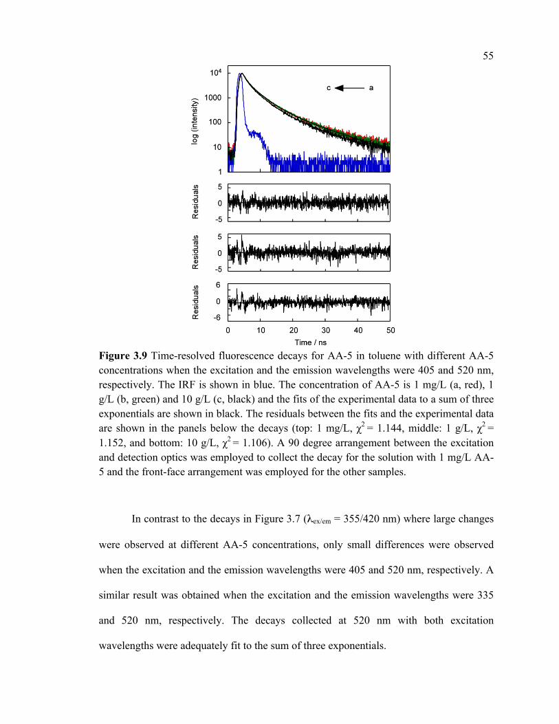
55

Figure 3.9 Time-resolved fluorescence decays for AA-5 in toluene with different AA-5 concentrations when the excitation and the emission wavelengths were 405 and 520 nm, respectively. The IRF is shown in blue. The concentration of AA-5 is 1 mg/L (a, red), 1 g/L (b, green) and 10 g/L (c, black) and the fits of the experimental data to a sum of three exponentials are shown in black. The residuals between the fits and the experimental data are shown in the panels below the decays (top: 1 mg/L, χ2 = 1.144, middle: 1 g/L, χ2 = 1.152, and bottom: 10 g/L, χ2 = 1.106). A 90 degree arrangement between the excitation and detection optics was employed to collect the decay for the solution with 1 mg/L AA-5 and the front-face arrangement was employed for the other samples.

In contrast to the decays in Figure 3.7 (λex/em = 355/420 nm) where large changes

were observed at different AA-5 concentrations, only small differences were observed

when the excitation and the emission wavelengths were 405 and 520 nm, respectively. A

similar result was obtained when the excitation and the emission wavelengths were 335

and 520 nm, respectively. The decays collected at 520 nm with both excitation

wavelengths were adequately fit to the sum of three exponentials.

56 Table 3.6 Recovered lifetimes and pre-exponential factors for the emission of AA-5 in toluene at different AA-5 concentrations (λex/em = 405/520 nm).a

[AA-5] mg/L τ1  / ns (A1)   τ2  / ns (A2)   τ3  / ns (A3)   <τ > / ns  

1 (3)b, c

1.26 ± 0.02 (0.60 ± 0.01)

3.51 ± 0.06 (0.35 ± 0.01)

9.5 ± 0.2 (0.051 ± 0.005)

2.46 ± 0.01

10 (4)b, c

1.21 ± 0.04 (0.60 ± 0.02)

3.5 ± 0.1 (0.35 ± 0.01)

9.4 ± 0.2 (0.050 ± 0.004)

2.41 ± 0.02

25 (2)b, c

1.23 ± 0.03 (0.60 ± 0.02)

3.5 ± 0.1 (0.35 ± 0.01)

9.5 ± 0.3 (0.050 ± 0.006)

2.43 ± 0.02

50 (3)b, c

1.23 ± 0.04 (0.61 ± 0.01)

3.50 ± 0.05 (0.35 ± 0.01)

9.4 ± 0.1 (0.051 ± 0.003)

2.42 ± 0.04

100 (3)b, d

1.24 ± 0.03 (0.61 ± 0.01)

3.50 ± 0.06 (0.34 ± 0.01)

9.3 ± 0.1 (0.052 ± 0.002)

2.43 ± 0.01

250 (2)b, d

1.15 ± 0.03 (0.57 ± 0.01)

3.43 ± 0.08 (0.37 ± 0.01)

9.3 ± 0.2 (0.057 ± 0.005)

2.45 ± 0.02

500 (2)b, d

1.22 ± 0.03 (0.58 ± 0.01)

3.53 ± 0.06 (0.36 ± 0.01)

9.4 ± 0.1 (0.059 ± 0.003)

2.54 ± 0.03

1000 (5)b, d

1.12 ± 0.08 (0.57 ± 0.02)

3.4 ± 0.2 (0.38 ± 0.01)

9.1 ± 0.3 (0.059 ± 0.004)

2.43 ± 0.07

2500 (2)b, d

1.05 ± 0.03 (0.54 ± 0.01)

3.29 ± 0.06 (0.39 ± 0.01)

8.9 ± 0.2 (0.064 ± 0.005)

2.43 ± 0.05

5000 (2)b, d

1.0 ± 0.1 (0.54 ± 0.01)

3.2 ± 0.1 (0.39 ± 0.01)

8.6 ± 0.2 (0.065 ± 0.003)

2.32 ± 0.09

10000 (4)b, d

1.02 ± 0.09 (0.59 ± 0.02)

3.1 ± 0.1 (0.35 ± 0.02)

8.2 ± 0.1 (0.057 ± 0.005)

2.18 ± 0.08

a, errors for the average of two independent experiments correspond to the average deviation or the propagation of individual error values, whichever is larger. Errors for more than two independent experiments correspond to the standard deviation. b, values in parenthesis correspond to the number of independent experiments. c, experiments were performed by using a 90 degree arrangement between the excitation beam and the detection optics. d, experiments were performed using the front-face sample holder.

In general, the average lifetimes obtained for the excited states in AA-5 that emit

at 520 nm were longer than the lifetimes obtained for the detection at 420 nm (Table 3.5,

Table 3.6 and Appendix A, Table A.1). Moreover, the average lifetimes obtained for the

excited states in AA-5 when the excitation and the emission wavelengths were 405 and

57 520 nm, respectively, were slightly shorter than that the lifetimes obtained when the

excitation and the emission wavelengths were 335 and 520 nm, respectively (Table 3.6

and Appendix A, Table A.1). These observations suggest that the different chromophores

are monitored at different combinations of excitation and emission wavelengths.

However, the chromophores that emit at 520 nm show some similarities on the trend for

the shortening of the average lifetimes with the increase of the AA-5 concentrations. In

Figure 3.10 and Figure 3.11, the average lifetimes decreased with the increase of the AA-

5 concentrations and this change for the average lifetimes did not dependent linearly on

the AA-5 concentration. There were two distinct regions for this dependence, containing

one platform region where a constant average lifetime was observed and one region

where the shortening of the average lifetime was observed.

At 520 nm, a constant average lifetime was observed over a wide range of AA-5

concentrations from 1 mg/L to 1 g/L. The individual lifetimes and their A values

remained the same in this region. The shortening of the average lifetimes was observed at

AA-5 concentrations higher than 1 g/L, where the three individual lifetimes were

shortened but their A values did not change significantly with the increase of AA-5

concentrations.

58

Figure 3.10 Dependence of the average lifetimes for the emission of AA-5 with the AA-5 concentrations when the excitation and the emission wavelengths were 405 and 520 nm, respectively: a, [AA-5] = 1 mg/L to 10 g/L; b, [AA-5] = 1 mg/L to 250 mg/L (red dots: experiments performed using a 90 degree arrangement between the excitation source and the detection system; blue squares: experiments performed using the front-face sample holder).

59

Figure 3.11 Dependence of the average lifetimes for the emission of AA-5 with the AA-5 concentrations when the excitation and the emission wavelengths were 335 and 520 nm, respectively: a, [AA-5] = 1 mg/L to 10 g/L; b, [AA-5] = 1 mg/L to 250 mg/L. (red dots: experiments performed using a 90 degree arrangement between the excitation source and the detection system; blue squares: experiments performed using the front-face sample holder).

3.2.3. Time-resolved emission spectra for AA-5 asphaltene

Time-resolved emission spectra (TRES) are the recovered emission spectra from

the time resolved fluorescence decays, where the intensities at specific wavelengths are

obtained from integrating the decays between different time intervals. TRES

measurements have the advantage over steady state fluorescence measurements that the

fluorescence spectrum for particular species at specific time intervals after the excitation

pulse is obtained. In the case of the steady-state spectrum the combined emission of all

60 species in solution is always obtained. An example of the time-resolved fluorescence

decays and TRES for an AA-5 sample is shown in Figure 3.12.

Figure 3.12 Time-resolved fluorescence decays (top) for 10 g/L AA-5 in toluene collected at 400 nm (a, red), 460 nm (b, blue), 520 nm (c, green) and 600 nm (d, black) when the excitation wavelength was 335 nm. The normalized TRES (bottom) obtained from integration for different time intervals: 0-5 ns (e, red), 5-10 ns (f, blue), 10-15 ns (g, green) and 15- 20 ns (h, black). The decays were collected with the front-face sample holder.

The time-resolved fluorescence decays for AA-5 samples were collected from 400

nm to 600 nm. Selected decays are shown in the upper panel of Figure 3.12 in order to

show the major differences between the decays. For example the decay collected at 400

nm showed a significantly faster decay than the decay collected at 460 nm. The bottom

panel of Figure 3.12 shows the spectra up to a time interval for which no further changes

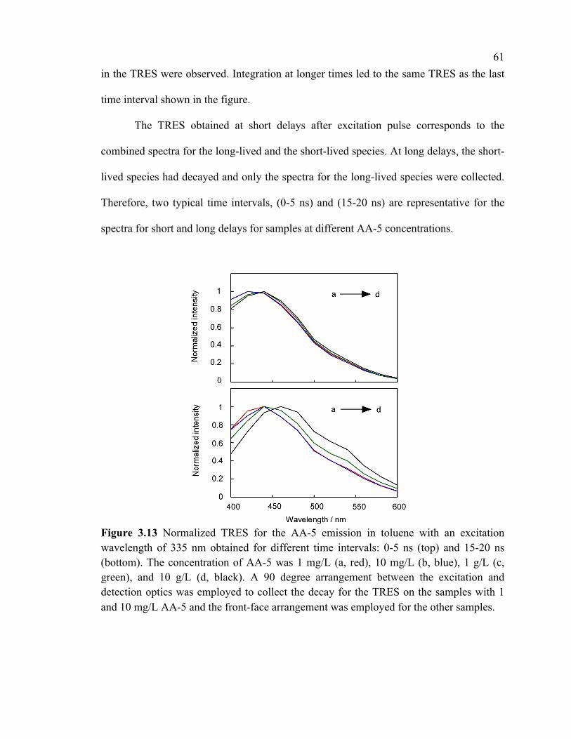
61 in the TRES were observed. Integration at longer times led to the same TRES as the last

time interval shown in the figure.

The TRES obtained at short delays after excitation pulse corresponds to the

combined spectra for the long-lived and the short-lived species. At long delays, the short-

lived species had decayed and only the spectra for the long-lived species were collected.

Therefore, two typical time intervals, (0-5 ns) and (15-20 ns) are representative for the

spectra for short and long delays for samples at different AA-5 concentrations.

Figure 3.13 Normalized TRES for the AA-5 emission in toluene with an excitation wavelength of 335 nm obtained for different time intervals: 0-5 ns (top) and 15-20 ns (bottom). The concentration of AA-5 was 1 mg/L (a, red), 10 mg/L (b, blue), 1 g/L (c, green), and 10 g/L (d, black). A 90 degree arrangement between the excitation and detection optics was employed to collect the decay for the TRES on the samples with 1 and 10 mg/L AA-5 and the front-face arrangement was employed for the other samples.

62 When the concentration of AA-5 was increased, the changes observed for the

TRES at different concentrations for different time intervals showed different trends. In

Figure 3.13, the TRES from the 0-5 ns time interval were slightly red shifted, while the

TRES from the 15-20 ns time interval had larger red shifts for the concentrated samples.

3.2.4 Quenching studies by nitromethane of the AA-5 asphaltene emission

MeNO2 is an organic molecule with a small size. It has low excitation energy and

has been used as a quencher to quench the excited states of PAHs.78 Figure 3.14 shows an

example of time-resolved fluorescence decays for AA-5 samples with the addition of

MeNO2. The decays became faster with the increase of quencher concentrations.

63

Figure 3.14 Time-resolved fluorescence decays for 1 g/L AA-5 in toluene with the addition of 0 mM (a, red), 28.2 mM (b, green), 71.7 mM (c, black) of MeNO2 when the excitation and emission wavelengths were 335 and 420 nm, respectively. The IRF is shown in blue. The fits of the experimental data to a sum of three exponentials are shown in black. The residuals between the fits and the experimental data are shown in the panels below the decays (top: 0 mM MeNO2, χ2= 1.134, middle: 28.2 mM MeNO2, χ2= 1.111, and low: 71.7 mM MeNO2, χ2= 1.098). The decays were collected with the front-face sample holder.

All decays were fit to the sum of three exponentials. An example of the changes

in individual lifetimes and their A values for 10 mg/L AA-5 with the addition of MeNO2

is shown in Figure 3.15 and Table B.1 in Appendix B. The similar changes in individual

lifetimes and their A values were obtained for 1 g/L AA-5 with the addition of MeNO2

(Appendix B, Table B.2).

64

Figure 3.15 Dependence of the lifetimes (top) and their A values (bottom) with the concentration of MeNO2 for a 10 mg/L AA-5 solution in toluene. The excitation and emission wavelengths were 335 and 420 nm, respectively (red: the shortest lifetime; blue: the medium lifetime; and green: the longest lifetime).

Individual lifetimes for the excited states of AA-5 were slightly shortened, and the

A1 value was increased at the expense of the other A values when the concentration of

MeNO2 was increased. The quenching plots were obtained by plotting the decay rate

constant (kobs) against the concentrations of MeNO2 (Equation 1.9). The slope of this plot

corresponds to the quenching rate constant, kq, and kobs is equal to the inverse of the

average lifetime. The quenching plots for AA-5 at two different concentrations are shown

in Figure 3.16.

65

Figure 3.16 Quenching plots for the emission of 1 g/L AA-5 in toluene (a, green) and 10 mg/L AA-5 in toluene (b, red) by MeNO2 when the excitation and emission wavelengths were 335 and 420 nm, respectively.

Slightly curved quenching plots were obtained. This curvature could indicate that

the time resolution of the single photon counter was reached at the higher quencher

concentrations. For this reason the kq values were obtained only from the linear portion

([MeNO2] = 0-55mM) of the quenching plots. The kq values obtained at different

excitation and emission wavelengths are summarized in Table 3.7.

Table 3.7 Quenching rate constants for AA-5 by MeNO2. a, b

[AA-5] kq /109 M-1s-1

λex/em = 335/420 nm λex/em = 335/520 nm λex/em = 405/520 nm 10 mg/L 7.3 ± 0.4 1.2 ± 0.2 0.87 ± 0.06

1 g/L 8.1 ± 0.4 1.2 ± 0.1 1.04 ± 0.09 a, quenching rate constants were obtained from the concentration range of MeNO2 between 0 and 55 mM. b, two independent experiments were performed. Errors for the average of two experiments correspond to the average deviation or the propagation of individual errors, whichever is larger.

No difference in the quenching efficiency was observed for AA-5 samples at two

different concentrations. Higher quenching rate constants were observed for the

66 chromophores that emit at 420 nm, suggesting that the MeNO2 quenches the

chromophores with high excited state energies more efficiently than those with low

excited state energies.

An example of TRES for the AA-5 emission in the absence and presence of

MeNO2 is shown in Figure 3.17.

Figure 3.17 Normalized TRES for 10 mg/L AA-5 in toluene (top panel) in the absence of MeNO2 for different time interval: 0-5 ns (a, red solid line) and 15-20 ns (c, green solid line); and in the presence 37 mM MeNO2 for different time intervals: 0-5 ns (b, red dash line) and 15-20 ns (d, green dash line). Normalized TRES for 1 g/L AA-5 in toluene (bottom panel) in the absence of MeNO2 for different time interval: 0-5 ns (e, blue solid line) and 15-20 ns (f, black solid line); and in the presence 19 mM MeNO2 for different time intervals: 0-5 ns (f, blue dash line) and 15-20 ns (g, black dash line). A 90 degree arrangement between the excitation and detection optics was employed to collect the decay for the TRES on the 10 mg/L AA-5 and the front-face sample holder was employed for 1 g/L AA-5.

67 When the relative intensities were compared, the emission intensities of chromophores

that emit at shorter wavelengths (e.g. 400 nm) were quenched more efficiently than the

chromophores that emit at longer wavelengths (e.g. 540 nm). Also, the chromophores

with long lifetimes (15-20 ns) were quenched more efficiently than those with short

lifetimes (0-5 ns). Therefore, the TRES results confirmed that MeNO2 quenches

chromophores in AA-5 solutions selectively.

3.3 Discussion

3.3.1 The dependence of fluorescence spectra of AA-5 asphaltene on the asphaltene

concentration

The fluorescence spectra for asphaltenes and oil samples were found to be

dependent on the concentration of the samples.41,42,45,47,60,65 A red shift of the

fluorescence spectra was observed when the concentration of the samples was increased.

A red shift in the fluorescence spectra is expected due to the energy transfer or

quenching of the chromophores in the asphaltenes or oil samples as the concentration of

chromophores is increased. At high concentrations, chromophores with different excited

state energies are close to each other and the electronic excitation energy can be

transferred from the chromophores with higher excited state energies to the

chromophores with the lower excited state energies. The latter chromophores emit at

longer wavelengths compared to the chromophores with high excited state energies. The

electronic excitation energy from the chromophores with high excited state energies can

be also quenched by non-fluorescent compounds. Both the energy transfer and quenching

68 will decrease the emission intensity for the chromophores emitting at short wavelengths,

resulting in a red shift of the fluorescence spectra.

A red shift of the fluorescence spectra can also be caused by self-absorption as

discussed in section 2.3.5. In Figure 3.2, a red shift of the fluorescence spectrum for 50

mg/L AA-5 was observed using a 90 degree arrangement between the excitation and

detection optics compared to the spectrum obtained using the front-face sample holder.

Therefore, the red shift might be an artifact for experiments done with a 90 degree

arrangement between the excitation and detection optics.42,45 In several literature reports,

the problem of self-absorption was pointed out and alternative methods, such as the use

of front face measurements, were employed to avoid this problem in the measurements of

fluorescence for concentrated crude oils or asphaltene samples.41,47,60,65 Front face

measurements can be achieved in different ways. First, a square cell can be orientated at

an angle other than 90 degree relative to the incident beam. Albuquerque et al. worked at

a 22 degree angle for the front face measurement.65 Second, front face measurement can

also be archived by using triangular cells, like the one that was employed in Pietraru et

al.’s work.41 In Albuquerque et al.’s and Pietraru et al.’s work, the shape of the

fluorescence emission spectra did not change substantially with the increase of the

asphaltene concentrations. “Front-surface mode” was mentioned to be used in the

fluorescence measurements of oil samples in some works.47,60 However, the authors did

not explain in detail how the “front-surface mode” operates. In these studies a large red

shifted and broad spectra were observed for the neat oils samples compare to the diluted

oil ones. However, without a detailed description of the experimental set-up one cannot

be assure that these red shifts are not due to the self-absorption artifact.

69 In the present work, the problem of self-absorption was solved by the usage of the

front-face sample holder. This design is different from other devices used in the literature

reports since not only the angle between the normal and incident beam is changed from

90 degree to 52 degree, but also the reflection of light is minimized by tilting the cell

backwards (Figure 2.1). As a result, the self-absorption effect was eliminated and the

shape of the fluorescence emission spectra did not change substantially with the increase

of the AA-5 concentrations (Figure 3.4). Only a slight red shift of the spectra was

observed for concentrated solutions (10 g/L). These results were consistent with

Albuquerque et al.’s and Pietraru et al.’s work.41,65

3.3.2 The dependence of fluorescence lifetimes on the concentration of AA-5

Time-resolved fluorescence experiments have been widely used to study crude

oils and asphaltenes, but different methods were used to analyze the fluorescence decays.

Wang et al.47 and Ralston et al.62 recovered individual lifetimes for the excited states in

crude oils or asphaltenes at different dilutions, and the individual lifetimes increased

significantly with the increase in dilution. In their experiments, the decays were fit to

mono- or the sum of two-exponentials with χ2 values of approximately 2. The authors

mentioned that the increase of the number of exponentials to three did not significantly

change the χ2 values, but they did not show the residuals for the fits. In the present work,

three or four lifetimes were required to achieve the acceptable χ2 values between 0.9 and

1.2. In Figure 3.6, the χ2 values were 1.359 and 0.989 for the decays were fit to the sum of

two- or three-exponentials, respectively. The trends observed in the previous reports47,62

and in this work are comparable from the qualitative point of view, but the method used

70 in this work provides more detailed information because of the appropriate χ2 values

obtained.

A different method used is the calculation of the average lifetimes based on the

individual lifetimes and their pre-exponential factors. This method is used to study the

fluorescence emission of all chromophores in crude oils or asphaltenes. For example,

crude oils with different concentrations of aromatic compounds were compared by their

average lifetimes.70 In this work, the average lifetimes of oil samples were increased as

the concentration of aromatic components decreased. The content of aromatic

components in this case was measured by high performance liquid chromatography

(HPLC). Thus, average lifetime measurements were employed to predict the

concentration of aromatic compounds in oil samples. In comparison, the analysis of

individual lifetimes is not comprehensive because some of the chromophores that have

longer lifetimes at low chromophore concentrations have shorter lifetimes at the higher

concentrations. Therefore, the average lifetime, which incorporates the emission of all

chromophores in asphaltenes, is particularly useful to study the aggregation behaviour at

various concentrations of asphaltenes.

A distribution of lifetimes was also used to analyze the fluorescence decays of

asphaltene.46 In this case, the fluorescence decays were fit to a series of exponential

functions, and up to 100 lifetime values were recovered. Histograms of lifetime

distribution were plot over the range of 0.1-10 ns, and the distribution maximums of

lifetime were reported. At similar experimental conditions, the present results (the

average lifetime) were comparable with the results obtained from distribution maximum

of lifetimes for asphaltenes. For example, at low concentration (16 mg/L asphaltenes),

71 one distribution maximum of lifetime was observed around 2.3 ns when the excitation

and emission wavelength were 467 and 511 nm, respectively.46 An average lifetime of

(2.41 ± 0.02) ns for the 10 mg/L AA-5 was obtained when the excitation and emission

wavelengths were 405 and 520 nm, respectively. The difference might be caused by

different asphaltene samples and the different excitation and emission wavelengths

employed. At high concentrations of asphaltene, ca. 80 mg/L asphaltene, two distribution

maximums of lifetime were reported around 0.4 and 2.3 ns.46 The short lived component

was attributed to the asphaltene aggregates by the authors. However, the author ignored a

local maximum around 10 ns, which was presented as a small shoulder peak in the

lifetime distribution. In the present work, a lifetime around 9 ns was always recovered.

The dependence of fluorescence lifetimes on the concentrations of crude oils or

asphaltenes has been reported by several researchers.14,46,47,62 Different analysis methods

lead to the similar results that the lifetimes of excited states in crude oils or asphaltenes

increase with increased dilution. Ralston et al. pointed out that asphaltenes had a dilution

limit of about 10 mg/L and the fluorescence lifetimes did not change with further

dilution.62 Qualitatively the present results agree with this report, where the individual

lifetimes and their A values were found to be constants for all the dilutions below 10

mg/L for all the emission wavelengths investigated. From these experiments one can

conclude that energy transfer is minimal between AA-5 molecules when the

concentration of AA-5 is below 10 mg/L. Thus, AA-5 molecules that fluoresce are

dispersed as a true solution at these low concentrations.

The shortening of lifetimes for the emission of asphaltene solutions are probably

due to two reasons. First, quenching can occur between the chromophores in close

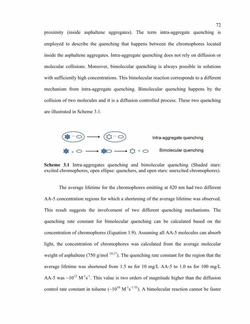
72 proximity (inside asphaltene aggregates). The term intra-aggregate quenching is

employed to describe the quenching that happens between the chromophores located

inside the asphaltene aggregates. Intra-aggregate quenching does not rely on diffusion or

molecular collisions. Moreover, bimolecular quenching is always possible in solutions

with sufficiently high concentrations. This bimolecular reaction corresponds to a different

mechanism from intra-aggregate quenching. Bimolecular quenching happens by the

collision of two molecules and it is a diffusion controlled process. These two quenching

are illustrated in Scheme 3.1.

Scheme 3.1 Intra-aggregates quenching and bimolecular quenching (Shaded stars: excited chromophores, open ellipse: quenchers, and open stars: unexcited chromophores).

The average lifetime for the chromophores emitting at 420 nm had two different

AA-5 concentration regions for which a shortening of the average lifetime was observed.

This result suggests the involvement of two different quenching mechanisms. The

quenching rate constant for bimolecular quenching can be calculated based on the

concentration of chromophores (Equation 1.9). Assuming all AA-5 molecules can absorb

light, the concentration of chromophores was calculated from the average molecular

weight of asphaltene (750 g/mol 14,17). The quenching rate constant for the region that the

average lifetime was shortened from 1.5 ns for 10 mg/L AA-5 to 1.0 ns for 100 mg/L

AA-5 was ~1012 M-1s-1. This value is two orders of magnitude higher than the diffusion

control rate constant in toluene (~1010 M-1s-1 53). A bimolecular reaction cannot be faster

73 than the rate for the encounter of the reagents. Therefore, the quenching that happened at

low concentrations of AA-5 is not caused by a collision between two molecules and

could only be due to two molecules in close contact at the time of excitation. The only

possibility is that the chromophores are quenched by other components inside the AA-5

aggregates.

The same calculation was employed for the lifetime shortening observed at higher

AA-5 concentrations (1 g/L-10 g/L). The estimated rate constant is of the same order of

magnitude as the diffusional rate constant and for this reason the data were plotted

according to Equation 1.9 (Figure B.1 in Appendix B). This reaction is likely to be due to

bimolecular quenching and it occurred for the entire excitation/emission wavelength

combinations studied (Table 3.8)

Table 3.8 Bimolecular quenching rate constants for the emission of AA-5 quenched by ground state AA-5.a

λex/em 335/420 nm 335/520 nm 405/520 nm

kq / M-1s -1 (3 ± 1) × 1010 (4.2 ± 0.5) × 109 (4.2 ± 0.2) × 109

a, errors were obtained from linear fit from Appendix B, Figure B.1.

3.3.3 Wavelength dependent aggregation pattern of AA-5 asphaltene

A difference in the shape of steady-state fluorescence spectra of AA-5 samples

was observed at different excitation wavelengths, confirming that AA-5 contains

different chromophores with different excited state energies (Figure 3.3). Therefore, the

behaviour of different chromophores with the increase in the AA-5 concentration can be

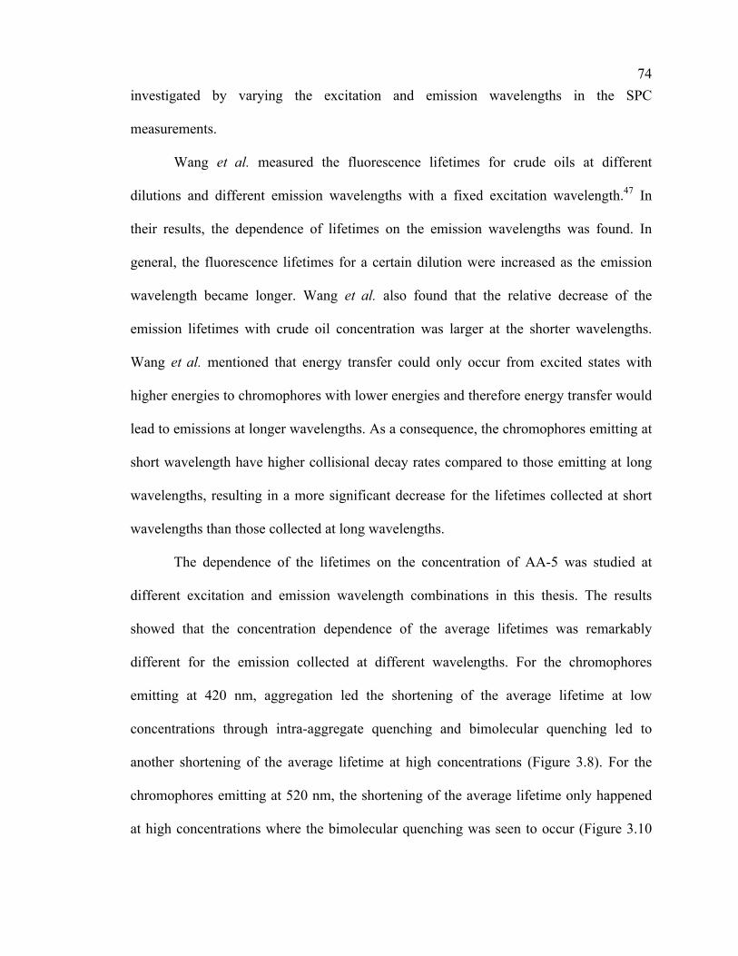
74 investigated by varying the excitation and emission wavelengths in the SPC

measurements.

Wang et al. measured the fluorescence lifetimes for crude oils at different

dilutions and different emission wavelengths with a fixed excitation wavelength.47 In

their results, the dependence of lifetimes on the emission wavelengths was found. In

general, the fluorescence lifetimes for a certain dilution were increased as the emission

wavelength became longer. Wang et al. also found that the relative decrease of the

emission lifetimes with crude oil concentration was larger at the shorter wavelengths.

Wang et al. mentioned that energy transfer could only occur from excited states with

higher energies to chromophores with lower energies and therefore energy transfer would

lead to emissions at longer wavelengths. As a consequence, the chromophores emitting at

short wavelength have higher collisional decay rates compared to those emitting at long

wavelengths, resulting in a more significant decrease for the lifetimes collected at short

wavelengths than those collected at long wavelengths.

The dependence of the lifetimes on the concentration of AA-5 was studied at

different excitation and emission wavelength combinations in this thesis. The results

showed that the concentration dependence of the average lifetimes was remarkably

different for the emission collected at different wavelengths. For the chromophores

emitting at 420 nm, aggregation led the shortening of the average lifetime at low

concentrations through intra-aggregate quenching and bimolecular quenching led to

another shortening of the average lifetime at high concentrations (Figure 3.8). For the

chromophores emitting at 520 nm, the shortening of the average lifetime only happened

at high concentrations where the bimolecular quenching was seen to occur (Figure 3.10

75 and 3.11). Either, these latter chromophores never form aggregates, or not all singlet

excited state lifetimes are shortened when the chromophores are aggregated. It is more

likely that these chromophores do not form aggregates because not only the average

lifetimes but also the individual lifetimes and their A values did not change with the

increase of the AA-5 concentrations. If some excited state lifetimes were shortened due to

the aggregation but some were not, the A values should have changed.

As a summary, some components of AA-5 form aggregates easily at low

concentrations (i.e. chromophores emitting at 420 nm). Other components of AA-5 may

form aggregates at higher concentrations or may not form aggregates for the

concentration range investigated. These results are inconsistent with the concept of a

critical concentration for aggregate formation. Therefore, the use of parameters such as

“CMC” or “CNAC” are not relevant to understand the mechanism for asphaltene

aggregation; asphaltenes do not have one concentration at which all its components start

to form aggregates.

3.3.4 The accessibility of nitromethane to different chromophores in AA-5

asphaltene aggregates

Ghosh et al. reported a fluorescence quenching experiment of asphaltene by

chloranil.69 They found that static quenching between chloranil and asphaltenes occurred,

in which only the fluorescence emission intensity was decreased with the increase of

quencher concentrations, but the average lifetimes of the asphaltene emission was

constant.

76 In the present work, MeNO2 was used as a quencher to quench the fluorescence

emission intensity and singlet excited state lifetimes for AA-5. Quenching requires

molecular contact between chromophores and quenchers. When asphaltenes form

aggregates, the chromophores are distributed in different locations inside the aggregates.

Some chromophores may cluster into the interior of the aggregates, and they may have

lower accessibilities to the quencher compared to those chromophores that are located on

the external surface of the aggregates or free in toluene. For this reason, quenching

studies can be used to reveal the location of a certain chromophore in a

microheterogenous solution. Different quenching efficiencies for MeNO2 were expected

for the emission of AA-5 as a monomer and when incorporated into AA-5 aggregates.

However, the same quenching rate constants were obtained for 10 mg/L and 1 g/L AA-5

with the addition of MeNO2 (Table 3.7). The lower AA-5 concentration was below the

threshold for which a shortening of the average lifetime was observed and therefore the

solutions only contained AA-5 monomers.

One possible explanation for the equal rate constants at different AA-5

concentrations is that the aggregation does not lead to the formation of a tight structure

making it possible for small molecules, like MeNO2, to easily access the interior of the

aggregate. Hence, the aggregates could not offer sufficient protection for the

chromophores located inside the aggregates. A second possible explanation is that only

the chromophores located on the surface of the aggregates or those free in toluene emit

and are readily accessible for quenching by MeNO2.

Moreover, the quenching rate constants obtained from different emission

wavelengths were very different. The chromophores emitting at 420 nm were quenched

77 more efficiently than those emitting at 520 nm (Table 3.7), indicating that MeNO2

selectively quench the chromophores with higher excited state energies over those with

lower excited state energies. Selective quenching by MeNO2 was reported previously,

where a different quenching efficiency was observed for alternant and non-alternant

PAHs.78 The basic idea was that MeNO2 quenched the alternant PAHs composed only of

six-membered rings more efficiently than nonalternant PAHs. This report might be

helpful for the identification of the composition for AA-5 samples, indicating that the

chromophores emitting at 420 nm might contain more alternant PAHs than the

chromophores emitting at 520 nm.

3.3.5 The usage of TRES as a tool to study the fluorescence of asphaltene

TRES is firstly reported to be employed in the study of asphaltene aggregates.

Instead of the combined emission measured in steady-state fluorescence spectra, the

spectra for the species with longer lifetime can be measured as a TRES. Thus, TRES can

be used to obtain information about the long lived species.

At a certain AA-5 concentration, a red shift of the TRES was observed at longer

decay times (Figure 3.12 bottom panel), indicating that chromophores emitting at longer

wavelengths have longer lifetimes. In Figure 3.13, the TRES for the 0-5 ns time window

corresponded to the combined emission for all emitting species in the AA-5 samples and

the TRES was slightly red shifted with the increase of the AA-5 concentration. The

TRES for the 0-5 ns time window is not very sensitive to changes in the AA-5

concentration, which is a similar result to that obtained from the steady-state fluorescence

spectra (Figure 3.4). In contrast, the TRES for the 15-20 ns time window are more

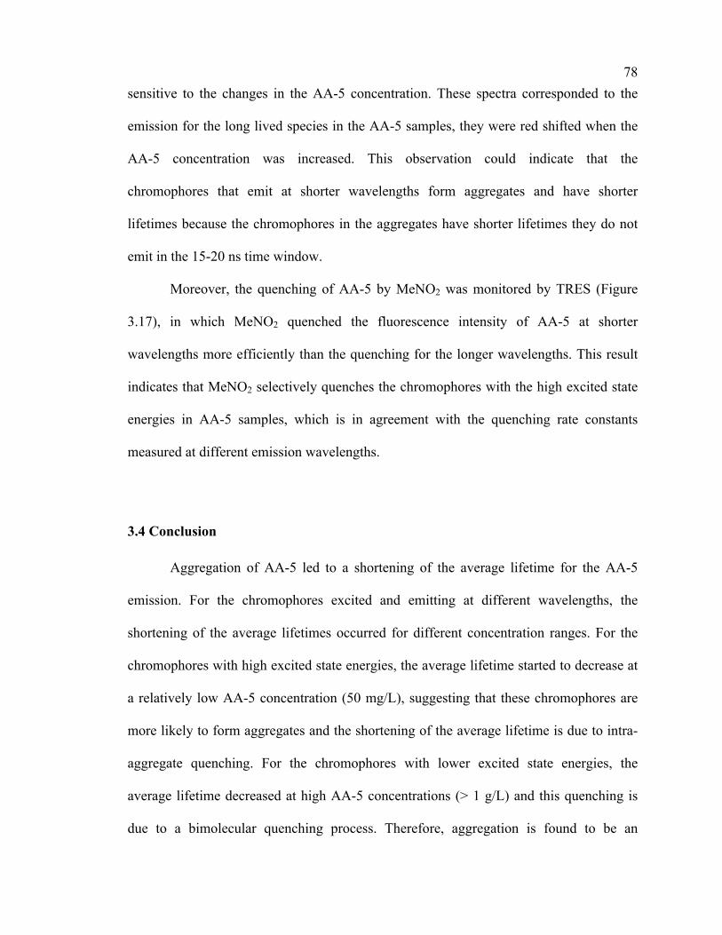
78 sensitive to the changes in the AA-5 concentration. These spectra corresponded to the

emission for the long lived species in the AA-5 samples, they were red shifted when the

AA-5 concentration was increased. This observation could indicate that the

chromophores that emit at shorter wavelengths form aggregates and have shorter

lifetimes because the chromophores in the aggregates have shorter lifetimes they do not

emit in the 15-20 ns time window.

Moreover, the quenching of AA-5 by MeNO2 was monitored by TRES (Figure

3.17), in which MeNO2 quenched the fluorescence intensity of AA-5 at shorter

wavelengths more efficiently than the quenching for the longer wavelengths. This result

indicates that MeNO2 selectively quenches the chromophores with the high excited state

energies in AA-5 samples, which is in agreement with the quenching rate constants

measured at different emission wavelengths.

3.4 Conclusion

Aggregation of AA-5 led to a shortening of the average lifetime for the AA-5

emission. For the chromophores excited and emitting at different wavelengths, the

shortening of the average lifetimes occurred for different concentration ranges. For the

chromophores with high excited state energies, the average lifetime started to decrease at

a relatively low AA-5 concentration (50 mg/L), suggesting that these chromophores are

more likely to form aggregates and the shortening of the average lifetime is due to intra-

aggregate quenching. For the chromophores with lower excited state energies, the

average lifetime decreased at high AA-5 concentrations (> 1 g/L) and this quenching is

due to a bimolecular quenching process. Therefore, aggregation is found to be an

79 inhomogeneous process in AA-5 solutions; not all species form aggregates at the same

concentration and different species have different aggregation behaviours.

Fluorescence quenching studies showed that MeNO2 had equal quenching

efficiency for the emission of AA-5 in diluted and concentrated solutions, but MeNO2

selectively quenched the chromophores with the high excited state energies over other

chromophores.

80

4. USE OF PYRENE AS AN EXTERNAL FLUORESCENT PROBE TO STUDY

THE AGGREGATION OF ASPHALTENES

Some of the results presented in this chapter have been published in the Photochemical &

Photobiological Sciences. Reproduced by permission of The Royal Society of Chemistry

(RSC) on behalf of the European Society for Photobiology, the European Photochemistry

Association, and RSC. This open access article can be accessed via the website (at

http://pubs.rsc.org/en/content/articlelanding/2014/pp/c4pp00069b).

4.1 Objectives

Fluorescence can be used to characterize the aggregation of asphaltenes by

exploring the intrinsic emission of asphaltenes as was presented in Chapter 3. A different

approach is to use externally added probes, which have different fluorescence properties

in different microenvironments.25,50 Py was chosen as an external probe to study the

aggregation of asphaltenes because Py might interact with a subset of the components of

asphaltenes through π−π stacking interactions.

The incorporation of Py into asphaltene aggregates could lead to quenching of the

fluorescence emission of Py because asphaltenes contain some components that have

lower excited state energies than Py. In addition, Py might be located in different

microenvironments. For example, Py could be located in the homogeneous toluene phase

or inside the asphaltene aggregates, leading to different lifetimes for the singlet excited

state of Py. The accessibility of small molecules to Py located in the various

microenvironments could also be different, and therefore the efficiency for the quenching

of the singlet excited state of Py by a quencher might be expected to be different. Such

81 differential quenching has been previously observed when the singlet excited state of Py

was incorporated into host systems such as cyclodoextrins,56 bile salt aggregates55,79 or

dendrocalixarenes.57 In the present study, MeNO2 was employed as a quencher for the

singlet excited state of Py78,80,81 in the presence of AA-5. The objective of the quenching

studies presented in this chapter was to investigate if Py was incorporated into the AA-5

aggregates and if the aggregates alter the accessibility of small molecules, i.e. the

quencher, to an aggregate incorporated probe.

4.2 Results

4.2.1 Steady-state fluorescence of pyrene

4.2.1.1 Fluorescence of pyrene in the presence of AA-5 asphaltene

AA-5 absorbs light over a wide range of the UV-visible spectrum, therefore, no

wavelength is available for the exclusive excitation of Py, without concomitantly exciting

the asphaltenes. The fluorescence emission spectra of Py in the presence of AA-5 were

obtained using an excitation wavelength of 337 nm, and the emission spectra of Py and

AA-5 overlapped. For this reason, the steady-state spectra correspond to the combined

spectra for the emission of Py and AA-5. The emission from AA-5 could be subtracted

from the combined emission spectrum when the AA-5 concentration was very low (top

panel in Figure 4.1). The resulting spectra were those for the Py emission and a decrease

in the Py fluorescence intensity was observed with the addition of AA-5. Such a decrease

could be either due to the quenching of the Py emission by AA-5 or it could be due to the

absorption of some of the photons of the excitation beam by AA-5 leading to a smaller

fraction of photons being absorbed by Py or it could be due to different

82 microenvironment for Py that leads to lower quantum yield. At high AA-5 concentrations

(10-100 mg/L) the AA-5 emission became prominent relative to the Py emission (bottom

panel in Figure 4.1). The Py emission was visible due to its vibrational structure

superimposed to the broad emission from AA-5. Such a large contribution of the AA-5

emission make it impossible to determine accurately the emission intensity of Py and any

further analysis from the steady-state emission spectra is not warranted.

. Figure 4.1 Top panel: fluorescence emission spectra for 20 µM Py in toluene (λex = 337 nm) with the addition of (a) 0 mg/L, (b) 1 mg/L, (c) 2 mg/L AA-5 when the emission of AA-5 was subtracted from the total spectrum. Bottom panel: normalized fluorescence emission spectra of 20 µM Py in toluene (λex = 337 nm) with the addition of (d) 0 mg/L, (e) 10 mg/L, (f) 50 mg/L and (g) 100 mg/L AA-5. The spectra were normalized at the maximum intensity. These spectra were not corrected for the Raman emission from the solvent because this emission was negligible. A 90 degree arrangement between the excitation source and detection optics was employed for all samples with the exception of the solution with 50 and 100 mg/L AA-5 for which the front face sample holder was used.

83

4.2.1.2 Quenching of the fluorescence of pyrene by nitromethane

The singlet excited state of Py is known to be quenched by MeNO2 in methanol

solutions with a rate constant of 3.6 × 109 M-1s-1.80 The fluorescence emission intensity

of Py in the absence of AA-5 was observed to decrease with the addition of MeNO2

(Figure 4.2).

Figure 4.2 Fluorescence emission spectra of 20 µM Py in toluene (λex = 337 nm) with the addition of (a) 0 mM, (b) 1.25 mM, (c) 2.5 mM and (d) 5 mM MeNO2. A 90 degree arrangement between the excitation source and detection optics was employed.

In Chapter 3, it was shown that the excited states in AA-5 are quenched by

MeNO2. The fluorescence of AA-5 and Py were both quenched by MeNO2. An example

of the typical fluorescence emission spectra of Py in the presence of AA-5 with

increasing MeNO2 concentrations is shown in Figure 4.3.

84

Figure 4.3 Fluorescence emission spectra of 20 µM Py (λex = 337 nm) in the presence of 500 mg/L AA-5 quenched by (a) 0 mM, (b) 0.97 mM, (c) 2.9 mM, (d) 4.8 mM and (e) 6.73 mM MeNO2. The front-face sample holder was employed for these measurements.

The fluorescence emission intensity of Py in the presence of AA-5 was observed

to decrease with the addition of MeNO2. Although the combined emission from Py and

AA-5 was obtained, the emission of Py was quenched more efficiently than the emission

from AA-5. This result is consistent with the longer excited state lifetimes for Py than for

asphaltene (see below).

4.2.2 Time-resolved fluorescence studies for the pyrene emission in the presence of

AA-5 asphaltene

4.2.2.1 Lifetime of pyrene in deaerated solutions

As described in Chapter 3, oxygen efficiently quenches excited states.48,51 The

singlet excited state lifetime of Py in aerated toluene was 18 ns, which was not very

different from the longest lifetime (ca. 7 ns) observed for the excited states of AA-5 in

aerated samples. After deaeration, an increase of the Py lifetime from 18 ns to 305 ns was

observed. This lifetime is much longer than the longest lifetimes (ca. 15 ns) for the

85 excited states of AA-5 in deaerated samples, making it easier to differentiate the Py

emission from the asphaltene emission. Therefore, all the time-resolved fluorescence

decays for samples containing Py were acquired using deaerated solutions.

The time-resolved fluorescence decay for Py in toluene was a straight line in the

semi-log plot and one lifetime was recovered for the Py singlet excited state. In contrast,

non-exponential decays were obtained with an initial fast component for the emission

decay of the Py-AA-5 solutions (Figure 4.4). The initial fast component increased as a

contribution of the total intensity when the AA-5 concentration was raised. This fast

component is due to the fluorescence emission from the excited states of AA-5, and/or

the Py inside the AA-5 aggregates (refer to section 4.3.1).

86

Figure 4.4 Time-resolved fluorescence decays for 20 µM Py in toluene in the presence of AA-5: (a, red) 0 mg/L, (b, blue) 10 mg/L, (c, green) 100 mg/L, (d, black) 500 mg/L and (e, purple) 1 g/L. The excitation and emission wavelengths were 335 and 391 nm, respectively. The fit of the experimental data are shown in black. The residuals between the fit for the sum of four exponentials (b-e) or for the mono-exponential function (a) and the experimental data are shown in the panels below the decays. The IRF is not shown because tail fits were employed (see 2.3.3). A 90 degree arrangement between the excitation source and detection optics was employed for all samples with the exception of the solutions with 100 and 500 mg/L AA-5 for which the front face sample holder was used.

87 The decays for the Py emission in the presence of AA-5 were fit to a sum of

exponentials. Usually, the fit to three or four lifetimes led to adequate residuals and χ2

values. The longest lifetime corresponds to the decay for the Py emission, while the other

shorter lifetimes are related to the fluorescence decays for AA-5.

The number of counts accumulated for the Py emission was decreased as the AA-

5 concentration was raised. The primary reason for this observation is that the AA-5

emission contributed more to the total emission as the AA-5 concentration increased. For

example, 10,000 accumulation counts for the channel with maximum intensity were

collected for the decay of Py in the absence of AA-5, and all the counts in this channel

were from the Py emission. In contrast, approximately 100 counts out of the total of

10,000 counts in the channel of maximum intensity were related to the Py emission in the

presence of 500 mg/L AA-5 (Figure 4.4). The low relative intensity for the Py emission

decreased the reliability of the fit and therefore values for the recovered lifetimes could

be less precise. A control experiment was performed with Py in the presence of 500 mg/L

AA-5, in which the decay was accumulated for 100,000 counts for the channel with

maximum intensity. In this case 1,000 counts were due to the Py emission. Comparison

of the decays with the two accumulation times showed that the recovered Py lifetimes

were the same. Therefore, for the experiments performed for Py in the presence of AA-5,

the total accumulation counts for the channel with maximum intensity was increased until

at least 100 counts were obtained for the longest lifetime due to Py emission.

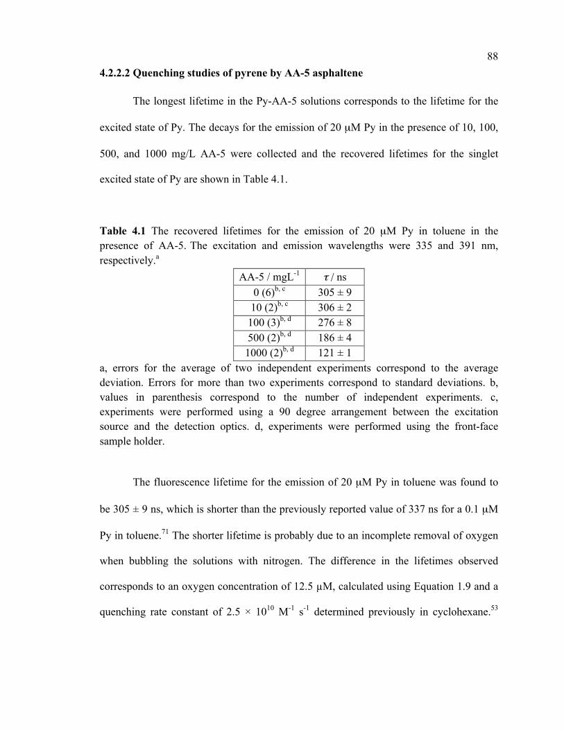
88 4.2.2.2 Quenching studies of pyrene by AA-5 asphaltene

The longest lifetime in the Py-AA-5 solutions corresponds to the lifetime for the

excited state of Py. The decays for the emission of 20 µM Py in the presence of 10, 100,

500, and 1000 mg/L AA-5 were collected and the recovered lifetimes for the singlet

excited state of Py are shown in Table 4.1.

Table 4.1 The recovered lifetimes for the emission of 20 µM Py in toluene in the presence of AA-5. The excitation and emission wavelengths were 335 and 391 nm, respectively.a

AA-5 / mgL-1 τ / ns 0 (6)b, c 305 ± 9 10 (2)b, c 306 ± 2

100 (3)b, d 276 ± 8 500 (2)b, d 186 ± 4 1000 (2)b, d 121 ± 1

a, errors for the average of two independent experiments correspond to the average deviation. Errors for more than two experiments correspond to standard deviations. b, values in parenthesis correspond to the number of independent experiments. c, experiments were performed using a 90 degree arrangement between the excitation source and the detection optics. d, experiments were performed using the front-face sample holder.

The fluorescence lifetime for the emission of 20 µM Py in toluene was found to

be 305 ± 9 ns, which is shorter than the previously reported value of 337 ns for a 0.1 µM

Py in toluene.71 The shorter lifetime is probably due to an incomplete removal of oxygen

when bubbling the solutions with nitrogen. The difference in the lifetimes observed

corresponds to an oxygen concentration of 12.5 µM, calculated using Equation 1.9 and a

quenching rate constant of 2.5 × 1010 M-1 s-1 determined previously in cyclohexane.53

89 This low oxygen concentration indicates that with nitrogen bubbling 99.4% of the total of

the oxygen in the aerated toluene sample ([O2]aerated = 2.1 mM)53 is removed.

A decrease of the Py lifetime from 305 ns in the absence of AA-5 to 121 ns in the

presence of 1 g/L AA-5 was observed, indicating that the singlet excited state of Py is

quenched by AA-5. A linear quenching plot was obtained for this quenching (Figure 4.5).

The quenching rate constant was (3.7 ± 0.2) × 109 M-1s-1 determined from the slope of the

quenching plot.

Figure 4.5 Quenching plot for the emission of 20 µM Py in toluene by AA-5, where the molecular weight of AA-5 is assumed to be 750 g/mol.17,19 The kobs values correspond to the inverse of the longest lifetimes recovered from the fluorescence decays of Py-AA-5 solutions. The line corresponds to the fit of the experimental data to Equation 1.9.

4.2.2.3 Quenching studies of pyrene by nitromethane in the absence and presence of

AA-5 asphaltene

The quenching experiments for the excited state of Py by MeNO2 were performed

in the presence of different concentrations of AA-5. The objective of these experiments

was to determine if the asphaltene aggregates provided a protection of incorporated Py

towards the quenching by MeNO2. Py species located in the interior of the aggregates are

90 expected to have a lower quenching efficiency than those excited Py species located in

the homogeneous phase.

In Chapter 3, it was shown that the change in the average lifetime of AA-5

emission with AA-5 concentrations was dependent on the excitation/emission

wavelengths used. For this reason, the lifetime dependence with the AA-5 concentration

was investigated at the excitation and emission wavelengths employed for Py

measurements (λex = 335 nm, λem = 391 nm) (Appendix C, Table C.1). The concentration

range of AA-5 investigated was between 10 mg/L and 5 g/L, and the front-face sample

holder was employed to measure the emission for the concentrated samples ([AA-5] ≥ 50

mg/L; refer to section 3.2.2.2 for details on the switch between sample holders).

One can notice in Figure 4.6 where the emission wavelength was 391 nm, that the

shortening of the average lifetime was more gradual in comparison to the trend shown in

Figure 3.8, where the emission wavelength was 420 nm. However, the chromophores that

emit at 391 nm showed the same pattern of the dependence of fluorescence lifetimes on

the concentration of AA-5 as the chromophores that emit at 420 nm. In particular, for

both emission wavelengths, two different regions for the shortening of the average

lifetimes were observed. One was observed at low AA-5 concentrations (around 50

mg/L), and a further shortening of the average lifetime was observed at high AA-5

concentrations (above 1 g/L). Two possible quenching mechanisms might be involved as

was discussed in section 3.3.2. The lifetime decrease at low AA-5 concentrations is due

to intra-aggregate quenching, while the lifetime shortening at high AA-5 concentrations

is due to the bimolecular quenching.

91

Figure 4.6 The changes of the average lifetimes for the emission of AA-5 when the excitation and emission wavelengths were 335 and 391 nm, respectively: a, [AA-5] = 10 mg/L to 5 g/L; b, [AA-5] = 10 mg/L to 200 mg/L (red dots: experiments performed using a 90 degree arrangement between the excitation beam and the detection optics, blue squares: experiments performed using the front-face sample holder).

In the presence of different concentrations of AA-5, the quenching of the

fluorescence of Py by MeNO2 was studied using SPC measurements. An example of the

fluorescence decays for the Py-AA-5 solutions with the addition of MeNO2 is shown in

Figure 4.7. The simultaneous quenching of the fluorescence of Py and AA-5 was

apparent in the steady-state experiments (Figure 4.3). However, in the SPC experiments

the quenching of the Py fluorescence can be studied separately from the quenching of the

AA-5 emission. The quenching of the Py emission was apparent as a shortening of the

longest lifetime in the decay (Fig. 4.7). The shortening of the AA-5 emission lifetimes

92 was not observable on the time scales used to detect the Py emission because the excited

state lifetimes for AA-5 are too short (< 15 ns).

Figure 4.7 Time-resolved fluorescence decays for 20 µM Py in the presence of 500 mg/L AA-5 quenched by MeNO2 when the excitation and emission wavelengths were 335 and 391 nm, respectively. The concentration of MeNO2 was 0 mM (a, red), 0.97 mM (b, blue), 2.9 mM (c, green), 4.8 mM (d, black) and 6.7 mM (e, purple). The fit of the experimental data are shown in black. The residuals between the sum of four exponential fits and the experimental data are shown in the panels below the decays. The front face sample holder was employed for all measurements.

93 Quenching plots were obtained by plotting the observed decay rate constants

against the concentrations of MeNO2, where the observed decay rate constants

correspond to the longest lifetimes, which are assigned to the Py emission. Figure 4.8

gives examples for the quenching plots for the quenching of the singlet excited state Py in

the presence of AA-5 by MeNO2.

Figure 4.8 Quenching plots for the emission of 20 µM Py by MeNO2 in the presence of 0 mg/L (○), 10 mg/L (□), 100 mg/L (◇) 500 mg/L (△) and 1 g/L (▽) AA-5 (λex/

em=335/391 nm). Quenching in the absence of AA-5 was studied for MeNO2 concentrations up to 16 mM. This last point, which falls on the linear relationship, is not included for clarity sake.

The quenching rate constants were calculated from the slopes of the quenching

plots (Equation 1.9). The quenching rate constants for the Py emission in the presence of

different concentrations of AA-5 were the same within experimental errors (Table 4.2).

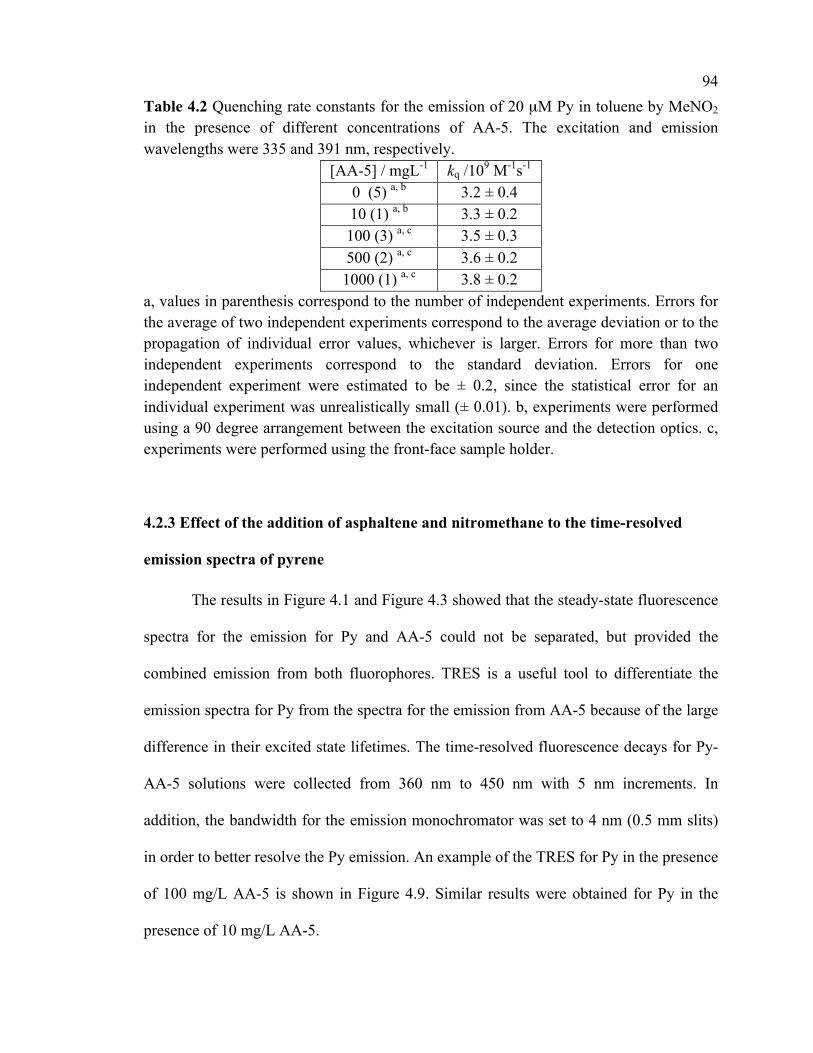
94 Table 4.2 Quenching rate constants for the emission of 20 µM Py in toluene by MeNO2

in the presence of different concentrations of AA-5. The excitation and emission wavelengths were 335 and 391 nm, respectively.

[AA-5] / mgL-1 kq /109 M-1s-1 0 (5) a, b 3.2 ± 0.4 10 (1) a, b 3.3 ± 0.2 100 (3) a, c 3.5 ± 0.3 500 (2) a, c 3.6 ± 0.2 1000 (1) a, c 3.8 ± 0.2

a, values in parenthesis correspond to the number of independent experiments. Errors for the average of two independent experiments correspond to the average deviation or to the propagation of individual error values, whichever is larger. Errors for more than two independent experiments correspond to the standard deviation. Errors for one independent experiment were estimated to be ± 0.2, since the statistical error for an individual experiment was unrealistically small (± 0.01). b, experiments were performed using a 90 degree arrangement between the excitation source and the detection optics. c, experiments were performed using the front-face sample holder.

4.2.3 Effect of the addition of asphaltene and nitromethane to the time-resolved

emission spectra of pyrene

The results in Figure 4.1 and Figure 4.3 showed that the steady-state fluorescence

spectra for the emission for Py and AA-5 could not be separated, but provided the

combined emission from both fluorophores. TRES is a useful tool to differentiate the

emission spectra for Py from the spectra for the emission from AA-5 because of the large

difference in their excited state lifetimes. The time-resolved fluorescence decays for Py-

AA-5 solutions were collected from 360 nm to 450 nm with 5 nm increments. In

addition, the bandwidth for the emission monochromator was set to 4 nm (0.5 mm slits)

in order to better resolve the Py emission. An example of the TRES for Py in the presence

of 100 mg/L AA-5 is shown in Figure 4.9. Similar results were obtained for Py in the

presence of 10 mg/L AA-5.

95

Figure 4.9 Normalized TRES for the emission of 20 µM Py in the presence of 100 mg/L AA when the excitation wavelength was 335 nm. The spectra in the top panel are those in the absence of MeNO2 obtained from the integration between different time windows: 0-38 ns (a, red solid), 38-76 ns (b, blue solid), 76-114 ns (c, green solid), 114-152 ns (d, black solid) and 152-190 ns (e, purple solid). The spectra in the bottom panel are those in the presence of 3.4 mM MeNO2 obtained from the integration between different time windows: 0-10 ns (a, red dash), 10-20 ns (b, blue dash), 20-30 ns (c, green dash), 30-40 ns (d, black dash) and 40-50 ns (e, purple dash). The experiments were performed using the front-face sample holder.

TRES provides more informative spectra than the steady-state fluorescence

spectra. At a short delay after the excitation pulse, the TRES showed the combined

emission from AA-5 and Py, which is similar to the steady-state fluorescence spectrum

(Figure 4.1). This TRES showed the structured emission from Py with a maximum at 390

nm on top of broad emission for AA-5. At longer delays after excitation, the short-lived

AA-5 component decayed and only the Py emission was collected in the TRES.

96 Similarly, in the presence of MeNO2 the TRES at short delays mainly showed the

emission from AA-5 where the Py emission appears as weak structured bands. As the

delay was increased the Py emission became more defined. The structured spectra for Py

around 370 to 400 nm became more clear and the intensities of broad band for AA-5

around 400 to 450 nm were decreased when the delay time became longer, consistent

with the smaller contribution from the short lived emission of AA-5.

4.3 Discussion

4.3.1 The changes of the fluorescence lifetime of pyrene in different environments

The objective of this work was to characterize the possible binding between Py

and asphaltene aggregates through π−π stacking interactions. It is known that the singlet

excited state lifetime of Py changes when it is incorporated into host systems. The

increase of fluorescence lifetime of Py was observed when it was incorporated into most

host systems such as sodium dodecyl sulfate (SDS) micelles, bile salt aggregates and

cyclodextrins.25,59,82-85 It was also observed that the binding between Py and some host

systems, such as the micelle of dendro-calixarene, led to a shortening of the fluorescence

lifetime.57 The lengthening of lifetime could be due to the increased in the rigidity around

Py provided by the host system, and a reduction of collisional interactions between the

excited state Py and the dissolved oxygen and other quenching impurities in the bulk

solution. The shortening of lifetime of Py (from 132 ns to 18 ns) was found to be due to

the interaction of the singlet excited state of Py with the dendro-calixarene when Py was

complexed to this host.57 Therefore, the measurement of Py lifetimes in the presence of

97 AA-5 is the tool employed to investigate the possible binding of Py to the AA-5

aggregates.

From the average lifetime studies of AA-5, it is known that some components in

AA-5 form aggregates at low concentrations (< 100 mg/L) (see section 3.3.2 and section

4.2.2.3). The fluorescence lifetime of Py was collected at high AA-5 concentration (ca. 1

g/L) for which the presence of AA-5 aggregates was detected. In the present work, the

fluorescence of Py showed a high sensitivity to the presence of AA-5 aggregates, the Py

lifetime decreased from 305 ns to 121 ns when the concentration of AA-5 was 1 g/L. The

changes of fluorescence lifetime of Py suggest an interaction between Py and AA-5. Two

possibilities exist for the shortening of the Py lifetime: i) incorporation into the AA-5

aggregate or ii) bimolecular quenching of the excited state Py in the homogenous phase

by AA-5.

Several studies on the incorporation of fluorescent probes into host systems

showed that the excited state of the probe decayed with two different lifetimes. The

difference is due to the probe partitioning between two different environments, one

lifetime is assigned to the fluorescence of probe free in the solvent and the other lifetime

is assigned to the fluorescence of probe located inside the host system.25 Therefore, more

than one lifetime is expected for the excited state of Py in the presence of AA-5

aggregates. In the present work, only one long lifetime assigned to the Py emission was

recovered from the fluorescence decays for Py-AA-5 solutions. The other shorter

lifetimes are assigned to AA-5 emission. This result suggests that all the emission come

from Py located in the same environment. The possibilities to be considered are: i) all the

Py molecules are located inside the AA-5 aggregates. ii) Py is partitioned into two

98 different environments. The long lived component corresponds to portion of Py free in

toluene and the emission of Py in the aggregate cannot be detected. iii) all the Py

molecules are located in toluene.

It is unlikely that all Py molecules are located inside the AA-5 aggregates. In the

present work, a shortening of the Py emission lifetime from 305 ns to 276 ns was

observed in the presence of 100 mg/L AA-5 solutions. If the lifetime of 276 ns is

assigned to the emission of Py located inside the aggregates, a constant lifetime is

expected to be obtained because further increases in the concentration of host molecules

will not affect the Py located inside the host system. For example, the fluorescence

lifetime of Py located inside dendro-calixarene micelles was 18 ns at different

concentration of dendro-calixarene.57 However, a continuous decrease (from 305 ns to

121 ns) in the fluorescence lifetime of Py was observed with the increase of AA-5

concentration (Table 4.1). This observation suggests that the emissive Py species is

located in an environment where it senses the increase in the total AA-5 concentration.

This observation is inconsistent with Py being located inside an aggregate where its

lifetime should not depend on how many other aggregates are present in solution.

Therefore, it is unlikely that all Py molecules are located inside the AA-5 aggregates.

It is possible that Py forms complexes with AA-5 aggregates and Py molecules

are partitioned between two different environments, i.e. the aggregates and the

homogenous phase. The Py molecules that are free in toluene have a long lifetime and

these species are detected as the long lived component for the fluorescence decays of the

Py-AA-5 solutions. On the other hand, the Py molecules incorporated into AA-5

aggregates can have a “hidden” lifetime, which could be due to two different

99 mechanisms. First, a tight complex can be formed between the ground state of Py and

AA-5 molecules in the aggregates, in which case static quenching can occur during

excitation. In this case, Py does not emit and it is not detectable in the SPC experiments.

For the static mechanism, a decrease in the steady-state intensity of the fluorophore is

observed (see section 1.2.1.5). However this experiment is not possible because the Py

and AA-5 emission spectra overlap. Second, the Py excited state is formed in the

aggregate but its lifetime is shorter than observed for Py in solution. As mentioned above

the continuous decrease in the lifetime of long lived Py fluorescence species is not due to

its incorporation into the aggregates. It is also reasonable to expect a shorter lifetime for

the aggregate incorporated Py because of the presence of chromophores with excited state

energies lower than the excited state energy for Py. However, no intermediate Py lifetime

between the lifetime for Py in toluene and the lifetimes for AA-5 was recovered at any

AA-5 concentrations. Therefore, if Py is incorporated into the aggregates its excited state

lifetime is of the order of the lifetimes for the emission of AA-5. In any event not all Py

can be incorporated into the aggregates because of the presence of the long lived Py

emission which is assigned to the emission of Py in toluene.

4.3.2 The quenching of the fluorescence lifetime of pyrene in the presence AA-5

asphaltene by nitromethane

The results discussed above suggest that either Py is not incorporated into the

AA-5 aggregates or that Py located inside the aggregates are not easily detected.

Quenching studies provides the information about the location of emissive Py species and

100 supported this assignment. Usually, aggregates act as a host system that can protect the

excited state of an incorporated fluorescence probe from external quenchers. A smaller

quenching rate constant is expected for the excited state Py located inside the aggregates

compared to Py that is free in solution. The experimental results showed that the

quenching rate constants did not change within error when the concentrations of AA-5

were increased from 0 to 1 g/L (Table 4.2), indicating that the presence of AA-5

aggregates does not offer any protection for the emissive Py from quenchers. Therefore,

the results of the quenching experiments are consistent with the assignment that the long

lived species corresponds to Py molecules free in toluene.

One should notice that the decay rate constants calculated in the quenching

studies were based on the longest lifetime recovered from the decays of Py-AA-5

solutions. Therefore the quenching studies only provide information on this species,

which is not protected from quenching. Any Py that might be in the aggregates is not

detectable in the SPC experiments and therefore is not involved in the quenching studies.

Based on the experimental results, the detectable Py are located in the

homogeneous phase and no Py is detected inside the AA-5 aggregates. These results are

probably a reflection of the fact that toluene is a good solvent for Py. In contrast, in

aqueous solutions, Py is readily incorporated into host systems with hydrophobic

environments, where the host system provides a protection of the excited state of Py from

quenching.25,50 In the organic phase, Py was found to interact with other aromatic systems

via π−π interactions.59 The fact that a substantial amount of Py is located in the

homogeneous phase in the presence of AA-5 suggests that π−π stacking, if it occurs is

101 weak. Therefore, Py is not a good probe to study asphaltene aggregation because it could

not be efficiently incorporated into the aggregates.

4.3.3 The quenching of the fluorescence lifetime of pyrene by AA-5 asphaltene

As discussed above, the emission of Py located in toluene is quenched by AA-5

via a bimolecular reaction. The quencher might be AA-5 monomers and/or AA-5

aggregates. If only the AA-5 monomers play the role of quencher, a curved quenching

plot with a downward curvature is expected because the quencher concentration would

not increase linearly with the AA-5 concentration as some AA-5 monomers would be

incorporated into aggregates. A curved quenching plot with a downward curvature is also

expected if AA-5 aggregates participate in the quenching process with an equal or lower

quenching efficiency than the quenching efficiency for AA-5 monomers. However, linear

quenching plots were obtained (Figure 4.5) in the present work. One possible explanation

is that AA-5 aggregates quench the emission of Py with a higher quenching efficiency

than AA-5 monomers, resulting in a linear quenching plot by coincidence. Another

possible explanation is that the effective components in AA-5 that quench the

fluorescence of Py do not form aggregates at the concentration range investigated.

In the present work, the quenching rate constant was determined to be (3.7 ± 0.2)

× 109 M-1s-1, which is lower than the diffusion control rate constant in toluene (1.1 x 1010

M-1s-1) at 20oC.53 The highest possible quenching rate constant for a bimolecular process

in solution is the one for a diffusion controlled process. Assuming that AA-5 quenches

the excited state of Py with the highest possible rate constant, at least one third of the

102 AA-5 components quench Py. Any lower fraction of AA-5 would lead to a rate constant

above the diffusion controlled limit, a situation that is not possible. In the early literature,

Nicodem worked on the quenching of Py by petroleum.71 The decay rate constants for the

fluorescence of Py were found to be proportional in a linear fashion to the concentration

of crude oil. The quenching rate constant was reported as (3.03 ± 0.06) × 109 petroleum

fraction-1s-1 but this unit was not defined. Since the literature value and the value reported

in the present work are different in units, a direct comparison cannot be made.

4.4 Conclusion

Py was employed as an external fluorescent probe to explore the importance of π-

π interactions between the Py and asphaltenes. Only one fluorescence lifetime was

recovered for the Py emission, which is assigned to Py that is free in the homogeneous

solvent. No evidence was observed for the complexation between Py and AA-5

aggregates, which means that either the complexes are not detectable with the techniques

employed or, more likely, that Py is not incorporated into AA-5 aggregates. This result

indicates that π-π interaction might not be the predominate driving force for the

incorporation of small aromatic molecules into asphaltene aggregates when they are

solubilized in toluene.

103

5. SUMMARY

The combination of the use of complementary fluorescence techniques was

employed to study the aggregation of asphaltenes by exploring the intrinsic emission

from asphaltene solutions at different concentrations. Intra-aggregate quenching led to

the shortening of the average lifetime for the asphaltene emission. The chromophores

with high excited state energies manifested to be more likely to form aggregates at low

concentrations (ca. 50 mg/L). The chromophores with lower excited state energies did not

aggregate for the concentration range investigated. Therefore, there is no critical

concentration at which asphaltenes aggregate. Different components in asphaltene

samples revealed different aggregation behaviours. The intrinsic asphaltene emission was

quenched by MeNO2, where the accessibility of quenchers to the asphaltene monomers

and aggregates were the same. Thus, asphaltene aggregation does not lead to a tight

complex and small molecules, such as MeNO2, can easily access the interior of the

aggregates. In addition, the selective quenching of MeNO2 on asphaltene molecules could

be used to differentiate between chromophores with different excited state energies.

The fluorescence of an externally added Py was investigated in the presence of

asphaltenes. No emissive Py species from the interior of asphaltene aggregates were

detected. When the Py emission was quenched by MeNO2, the quenching efficiencies

determined for Py in the absence or the presence of asphaltene aggregates were the same.

These results suggest that Py is not incorporated into asphaltene aggregates and all the

emissive Py species are located in the toluene phase, since the access of small molecules

is not hindered. Therefore, π-π stacking is not dominant for the incorporation of small

aromatic hydrocarbons into asphaltene aggregates when asphaltenes are solubilized in

104 toluene. Other probes that might be interact with asphaltene aggregates through acid-base

interactions or hydrogen bonding might be explored to better probe the different

environments in the asphaltene aggregates.

The current results provide information on that the types of components that are

relevant for aggregation, and on the “compactedness” of asphaltene aggregates. This

information is fundamental in the development of strategies for breaking up of the

asphaltene aggregates. Furthermore, based on the current experiments, the optimum

experimental conditions could be determined for which the accessibility of small

molecules is enhanced, which could be very useful to designing new methods for the

hydrogenation of asphaltene.

105

6. REFERENCES

(1) Leffler, W. L. Petroleum Refining in Nontechnical Language-4th ed.; Penn Well Corporation: Tulsa, 2008. (2) Vassiliou, M. S. The A to Z of the Petroleum Industry; The Scarecrow Press, Inc.: Plymouth, 2009. (3) Alboudwarej, H.; Felix, J.; Taylor, S.; R., B.; Bremner, C.; Breough, C.; Skeates, C.; Baker, A.; Palmer, D.; Pattison, K.; Beshery, M.; Krawchuk, P.; Brown, G.; Triana, J. A. C.; Hathcock, R.; Koerner, K.; Hughes, T.; Kundu, D.; Cardenas, J. L.; West, C. Oilfield Review 2006, 18, 34-53. (4) Mullins, O. C.; Sheu, E. Y.; Hammami, A.; Marshall, A. G. Asphaltenes, Heavy Oils, and Petroleomics; Springer: New York, 2007. (5) National Energy Board: Calgary, 2010. (6) Yarranton, H. W.; Fox, W. A.; Svrcek, W. Y. Can. J. Chem. Eng. 2007, 85, 635-642. (7) Akbarzadeh, K.; Hammami, A.; Kharrat, A.; Zhang, D.; Allenson, S.; Creek, J.; Kabir, S.; Jamaluddin, A.; Marshall, A. G.; Rodgers, R. P.; Mullins, O. C.; Solbakken, T. Oilfield Review 2007, 19, 22- 43. (8) Long, R. B. In Chemsitry of Asphaltenes; Bunger, J. W., Li, N. C., Eds.; American Chemical Society: Washington, 1981, p 17. (9) Hammami, A.; Ratulowski, J. In Asphaltenes, Heavey Oils, and Petroleomics; Mullins, O. C., Sheu, E. Y., Hammami, A., Marshall, A. G., Eds.; Springer: New York, 2007, p 617. (10) Collins, C. In Methods in Biotechnology; Willey, N., Ed.; Humana Press Inc.: Totowa, 2007; Vol. 23, p 99. (11) Ancheyta, J.; Trejo, F.; Rana, M. S. Asphaltenes: Chemical Transformation during Hydroprocessing of Heavy Oils; CRC Press: Boca Raton, 2009. (12) Mullins, O. C. Energy Fuels 2010, 24, 2179-2207. (13) Dechaine, G. P.; Gray, M. R. Energy Fuels 2010, 24, 2795-2808. (14) Mullins, O. C. Energy Fuels 2009, 23, 2845-2854.

106 (15) Speight, J. G.; Moschopedis, S. E. In Chemistry of Asphaltenes; Bunger, J. W., Li, N. C., Eds.; American Chemical Society: Washington, 1981, p 1. (16) Pinkston, D. S.; Duan, P.; Gallardo, V. A.; Habicht, S. C.; Tan, X.; Qian, K.; Gray, M. R.; Mullen, K.; Kenttamaa, H. I. Energy Fuels 2009, 23, 5564-5570. (17) Groenzin, H.; Mullins, O. C. J. Phys. Chem. A 1999, 103, 11237-11245. (18) Groenzin, H.; Mullins, O. C. Energy Fuels 2000, 14, 677-684. (19) Ruiz-Morales, Y. R., Mullins, O. C. Energy Fuels 2008, 23, 1169-1177. (20) Zajac, G. W.; Sethi, N. K.; Joseph, J. T. Scanning Microscopy 1994, 8, 423-426. (21) Sharma, A.; Groenzin, H.; Tomita, A.; Mullins, O. C. Energy Fuels 2002, 16, 490-496. (22) Ruiz-Morales, Y.; Wu, X.; Mullins, O. C. Energy Fuels 2007, 21, 944-952. (23) Agrawala, M.; Yarranton, H. W. Ind. Eng. Chem. Res. 2001, 40, 4664-4672. (24) Sheu, E. Y. J. Phys. Condens. Matter 1996, 8, 125-141. (25) Kalyanasundaram, K. Photochemistry in Microheterogeneous Systems; Academic Press: Orlando, 1987. (26) Dickie, J. P.; Yen, T. F. Anal. Chem. 1967, 39, 1847-1852. (27) Kuznicki, T.; Masliyah, J. H.; Bhattacharjee, S. Energy Fuels 2008, 22, 2379-2389. (28) Makhonin, G. M.; Petrov, A. A. Chem. Technol. Fuels Oils 1975, 11, 942-946. (29) Shirokoff, J. W.; Siddiqui, M. N.; Ali, M. F. Energy Fuels 1997, 11, 561-565. (30) Strausz, O. P.; Mojelsky, T. W.; Lown, E. M. Fuel 1992, 71, 1355-1363. (31) Murgich, J.; Abanero, J. A.; Strausz, O. P. Energy Fuels 1999, 13, 278-286. (32) Yarranton, H. W. J. Dispersion Sci. Technol. 2005, 26, 5-8.

107 (33) Long, J.; Xu, Z.; Masliyah, J. H. Langmuir 2007, 23, 6182-6190. (34) Rogel, E.; Leon, O.; Torres, G.; Espidel, J. Fuel 2000, 79, 1389-1394. (35) Monte, M. B. M.; Coelho, R. R.; Middea, A. Pet. Sci. Technol. 2004, 22, 991-1001. (36) Mostowfi, F.; Indo, K.; Mullins, O. C.; McFarlane, R. Energy Fuels 2008, 23, 1194-1200. (37) Andreatta, G.; Goncalves, C. C.; Buffin, G.; Bostrom, N.; Quintella, C. M.; Arteaga-Larios, F.; Perez, E.; Mullins, O. C. Energy Fuels 2005, 19, 1282-1289. (38) Zeng, H.; Song, Y. Q.; Johnson, D. L.; Mullins, O. C. Energy Fuels 2009, 23, 1201-1208. (39) Betancourt, S. S.; Ventura, G. T.; Pomerantz, A. E.; Viloria, O.; Dubost, F. X.; Zuo, J.; Monson, G.; Bustamante, D.; Purcell, J. M.; Nelson, R. K.; Rodgers, R. P.; Reddy, C. M.; Marshall, A. G.; Mullins, O. C. Energy Fuels 2009, 23, 1178-1188. (40) Freed, D. E.; Lisitza, N. V.; Sen, P. N.; Song, Y. Q. In Asphaltenes, HeaVy Oils and Petroleomics; Mullins, O. C., Sheu, E. Y., Hammami, A., Marshall, A. G., Eds.; Springer: New York, 2007, p 279. (41) Pietraru, G.-M.; Cramb, D. T. Langmuir 2003, 19, 1026-1035. (42) Ghosh, A. K.; Srivastava, S. K.; Bagchi, S. Fuel 2007, 86, 2528-2534. (43) Schneider, M. H.; Andrews, A. B.; Mitra-Kirtley, S.; Mullins, O. C. Energy Fuels 2007, 21, 2875-2882. (44) Goncalves, S.; Castillo, J. A.; Fernandez, A.; Acevedo, S. In 19th Congress of the International Commission for Optics: Optics for the Quality of Life; 1 ed.; SPIE: 2004; Vol. 4829, p 829-830. (45) Goncalves, S.; Castillo, J.; Fernandez, A.; Hung, J. Fuel 2004, 83, 1823-1828. (46) Souza, R. S.; Nicodem, D. E.; Garden, S. J.; Correa, R. J. Energy Fuels 2010, 24, 1135-1138. (47) Wang, X.; Mullins, O. C. Appl. Spectrosc. 1994, 48, 977-984. (48) Lakowicz, J. R. Principles of Fluorescence Spectroscopy, Third Edition; Springer: New York, 2006.

108 (49) Kalyanasundaram, K.; Thomas, J. K. J. Am. Chem. Soc. 1977, 99, 2039-2044. (50) Bohne, C.; Redmond, R. W.; Scaiano, J. C. In Photochemistry in Organized and Constrained Media; Ramamurthy, V., Ed.; VCH Publishers: New York, 1991, p 79. (51) Wardle, B. Principles and Applications of Photochemistry; John Wiley, 2009. (52) Hollas, M.; Chung, M.-A.; Adams, J. J. Phys. Chem. B. 1998, 102, 2947-2953. (53) Murov, S. L.; Carmichael, I.; Hug, G. L. Handbook of Photochemistry; Marcel Dekker, INC.: New York, 1993. (54) Xu, W.; Demas, J. N.; DeGraff, B. A.; Whaley, M. J. Phys. Chem. 1993, 97, 6546-6554. (55) Ju, C.; Bohne, C. Photochem. Photobiol. 1996, 63, 60-67. (56) Dyck, A. S. M.; Kisiel, U.; Bohne, C. J. Phys. Chem. B 2003, 107, 11652-11659. (57) Yihwa, C.; Kellermann, M.; Becherer, M.; Hirsch, A.; Bohne, C. Photochem. Photobiol. Sci. 2007, 6, 525-531. (58) Kobayashi. N.; Saito, R. H., H.; Hino, Y.; Ueno, A. Osa, T. J. Chem. Soc. Perkin Trans. 2 1983, 1031. (59) Leyton, P.; Sanchez-Cortes, S.; Garcia-Ramos, J. V.; Domingo, C.; Campos-Vallette, M.; Saitz, C.; Clavijo, R. E. J. Phys. Chem. B 2004, 108, 17484-17490. (60) Downare, T. D.; Mullins, O. C. Appl. Spectrosc. 1995, 49, 754-764. (61) Mullins, O. C.; Mitra-Kirtley, S.; Zhu, Y. Appl.Spectrosc. 1992, 46, 1405-1411. (62) Ralston, C. Y.; Mitra-Kirtley, S.; Mullins, O. C. Energy Fuels 1996, 10, 623-630. (63) Ryder, A. G. Appl. Spectrosc. 2002, 56, 107-116. (64) Wade, D. A.; Torres, P. A.; Tucker, S. A. Anal. Chim. Acta 1999, 397, 17-31.

109 (65) Albuquerque, F. C.; Nicodem, D. E.; Rajagopal, K. Appl. Spectrosc. 2003, 57, 805-810. (66) Merino-Garcia, D.; Andersen, S. I. Pet. Sci. Technol. 2003, 21, 507-525. (67) Al-Muhareb, E.; Morgan, T. J.; Herod, A. A.; Kandiyoti, R. Pet. Sci. Technol. 2007, 25, 81-91. (68) Ryder, A. G. Appl. Spectrosc. 2004, 58, 613-623. (69) Ghosh, A. K.; Bagchi, S. Energy Fuels 2008, 22, 1845-1850. (70) Ryder, A. G.; Glynn, T. J.; Feely, M.; Barwise, A. J. G. Spectrochim. Acta, Part A 2002, 58, 1025-1037. (71) Nicodem, D. E.; da Cunha, M. F. V.; Guedes, C. L. B. Appl. Spectrosc. 2000, 54, 1409-1411. (72) Arteaga-Larios, F. C., Ana; Perez, Elias Energy Fuels 2005, 19. (73) Yarranton, H. W.; Alboudwarej, H.; Jakher, R. Ind. Eng. Chem. Res. 2000, 39, 2916-2924. (74) Yin, C.-X.; Stryker, J. M.; Gray, M. R. Energy Fuels 2009, 23, 2600-2605. (75) Ware, W. R. J. Phys. Chem. 1962, 66, 455-458. (76) In EPL-Series Picosecond Pulsed Diode Lasers; Edinburgh Instruments Ltd.: Livingston, 2008; Vol. Issue 5, December 2008. (77) In EPLED 320- EPLED 360 Picosecond Pulsed Light Emitting Diodes; Edinburgh Instruments Ltd.: Livingston, 2008; Vol. Issue 1, March 2008. (78) Pandey, S.; Acree, W. E.; Cho, B. P.; Fetzer, J. C. Talanta 1997, 44, 413-421. (79) Chen, M.; Gratzel, M.; Thomas, J. K. J. Am. Chem. Soc. 1975, 97, 2052-2057. (80) Kleinman, M. H.; Bohne, C. In Molecular and Supramolecular Photochemistry; Ramamurthy, V., Schanze, K. S., Eds.; Marcel Dekker Inc.: New York, 1997; Vol. 1, p 391. (81) Fletcher, K. A.; Pandey, S.; Storey, I. K.; Hendricks, A. E.; Pandey, S. Anal. Chim. Acta 2002, 453, 89-96.

110 (82) Meyerhoffer, S. M.; McGown, L. B. Anal. Chem. 1991, 63, 2082-2086. (83) Ju, C.; Bohne, C. J. Phys. Chem. 1996, 100, 3847-3854. (84) Zhang, Y.; Liu, C.; Shi, W.; Wang, Z.; Dai, L.; Zhang, X. Langmuir 2007, 23, 7911-7915. (85) Yin, C.-X.; Tan, X.; Müllen, K.; Stryker, J. M.; Gray, M. R. Energy Fuels 2008, 22, 2465-2469.

111

Appendix A

Table A.1 Recovered lifetimes and pre-exponential factors for the emission of AA-5 in toluene at different concentrations (λex/em = 335/520 nm).a

[AA-5] mg/L τ1  / ns (A1)   τ2  / ns (A2)   τ3  / ns (A3)   <τ  > / ns  1

(4)b, c 1.27 ± 0.04 (0.55± 0.01)

3.53 ± 0.09 (0.39 ± 0.01)

9.3 ± 0.2 (0.059 ± 0.009)

2.62 ± 0.04

10 (6)b, c

1.26 ± 0.04 (0.54 ± 0.01)

3.52 ± 0.08 (0.39 ± 0.01)

9.4 ± 0.2 (0.063 ± 0.006)

2.65 ± 0.04

10 (2)b, d

1.22 ± 0.02 (0.57 ± 0.01)

3.54 ± 0.08 (0.38 ± 0.02)

9.7 ± 0.2 (0.054 ± 0.002)

2.55 ± 0.05

25 (2)b, c

1.24 ± 0.04 (0.55 ± 0.02)

3.58 ± 0.09 (0.40 ± 0.01)

9.7 ± 0.2 (0.060 ± 0.006)

2.66 ± 0.02

25 (2)b, d

1.19 ± 0.03 (0.54 ± 0.01)

3.45 ± 0.06 (0.40 ± 0.01)

9.4 ± 0.2 (0.060 ± 0.005)

2.58 ± 0.02

50 (2)b, c

1.23 ± 0.03 (0.52 ± 0.01)

3.51 ± 0.08 (0.41 ± 0.01)

9.5 ± 0.2 (0.069 ± 0.005)

2.74 ± 0.05

50 (2)b, d

1.12 ± 0.06 (0.53 ± 0.01)

3.41 ± 0.08 (0.40 ± 0.02)

9.4 ± 0.2 (0.066 ± 0.009)

2.58 ± 0.08

100 (2)b, d

1.06 ± 0.05 (0.51 ± 0.02)

3.4 ± 0.1 (0.42 ± 0.02)

9.2 ± 0.2 (0.071 ± 0.001)

2.60 ± 0.05

250 (2)b, d

1.03 ± 0.06 (0.50 ± 0.01)

3.35 ± 0.09 (0.43 ± 0.01)

9.2 ± 0.2 (0.072 ± 0.004)

2.62 ± 0.04

500 (2)b, d

1.08 ± 0.05 (0.51 ± 0.02)

3.4 ± 0.1 (0.42 ± 0.01)

9.2 ± 0.2 (0.070 ± 0.006)

2.63 ± 0.03

1000 (4)b, d

1.07 ± 0.03 (0.50 ± 0.01)

3.41 ± 0.03 (0.43 ± 0.01)

9.2 ± 0.1 (0.072 ± 0.003)

2.66 ± 0.05

2500 (2)b, d

1.02 ± 0.06 (0.50 ± 0.01)

3.3 ± 0.1 (0.42 ± 0.01)

9.1 ± 0.2 (0.076 ± 0.006)

2.61 ± 0.03

5000 (2)b, d

0.95 ± 0.07 (0.50 ± 0.01)

3.21 ± 0.07 (0.43 ± 0.01)

8.7 ± 0.1 (0.076 ± 0.006)

2.50 ± 0.05

10000 (2)b, d

0.90 ± 0.06 (0.51 ± 0.01)

3.08 ± 0.09 (0.42 ± 0.01)

8.3 ± 0.2 (0.073 ± 0.005)

2.35 ± 0.04

a, errors for the average of two independent experiments correspond to the average deviation or the propagation of individual error values, whichever is larger. Errors for more than two independent experiments correspond to the standard deviation. b, values in parenthesis correspond to the number of independent experiments. c, experiments were performed using a 90 degree arrangement between the excitation source and the detection optics. d, experiments were performed using the front-face sample holder.

112

Appendix B

Table B.1 Recovered lifetimes and pre-exponential factors for the emission of 10 mg/L AA-5 in toluene with the addition of MeNO2 (λex/em= 335/420 nm).a, b

[MeNO2] /mM τ1  / ns (A1)   τ2  / ns (A2)   τ3  / ns (A3)   <τ > / ns  0 0.80 ± 0.03

(0.69± 0.01) 2.7 ± 0.1

(0.27 ± 0.01) 8.3 ± 0.2

(0.042 ± 0.001) 1.63 ± 0.04

9.6 0.78 ± 0.02 (0.71 ± 0.01)

2.57 ± 0.05 (0.26 ± 0.01)

7.7 ± 0.1 (0.027 ± 0.001)

1.43 ± 0.02

19.0 0.75 ± 0.02 (0.72 ± 0.02)

2.32 ± 0.08 (0.26 ± 0.01)

7.4 ± 0.3 (0.023 ± 0.006)

1.31 ± 0.03

37.2 0.70 ± 0.03 (0.76 ± 0.01)

2.1 ± 0.1 (0.22 ± 0.01)

7.6 ± 0.4 (0.0122 ± 0.0001)

1.11 ± 0.03

54.8 0.66 ± 0.04 (0.78 ± 0.03)

1.9 ± 0.1 (0.21 ± 0.03)

7.2 ± 0.3 (0.0116 ± 0.0003)

1.00 ± 0.03

79.9 0.61 ± 0.01 (0.81 ± 0.01)

1.84 ± 0.05 (0.17 ± 0.01)

7.1 ± 0.2 (0.0108 ± 0.0001)

0.891 ± 0.006

111.4 0.59 ± 0.02 (0.87 ± 0.02)

1.9 ± 0.1 (0.12 ± 0.02)

7.5 ± 0.5 (0.0103 ± 0.0002)

0.82 ± 0.03

a, errors correspond to the standard deviation. b, experiments were performed using a 90 degree arrangement between the excitation source and the detection optics.

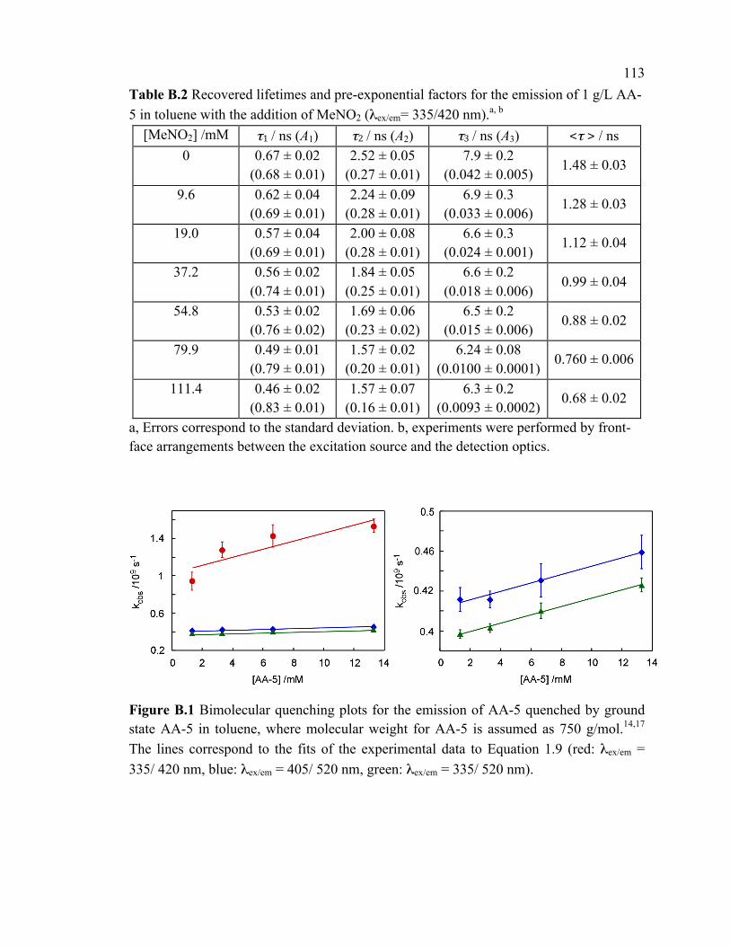
113 Table B.2 Recovered lifetimes and pre-exponential factors for the emission of 1 g/L AA-5 in toluene with the addition of MeNO2 (λex/em= 335/420 nm).a, b

[MeNO2] /mM τ1  / ns (A1)   τ2  / ns (A2)   τ3  / ns (A3)   <τ > / ns  0 0.67 ± 0.02

(0.68 ± 0.01) 2.52 ± 0.05

(0.27 ± 0.01) 7.9 ± 0.2

(0.042 ± 0.005) 1.48 ± 0.03

9.6 0.62 ± 0.04 (0.69 ± 0.01)

2.24 ± 0.09 (0.28 ± 0.01)

6.9 ± 0.3 (0.033 ± 0.006)

1.28 ± 0.03

19.0 0.57 ± 0.04 (0.69 ± 0.01)

2.00 ± 0.08 (0.28 ± 0.01)

6.6 ± 0.3 (0.024 ± 0.001)

1.12 ± 0.04

37.2 0.56 ± 0.02 (0.74 ± 0.01)

1.84 ± 0.05 (0.25 ± 0.01)

6.6 ± 0.2 (0.018 ± 0.006)

0.99 ± 0.04

54.8 0.53 ± 0.02 (0.76 ± 0.02)

1.69 ± 0.06 (0.23 ± 0.02)

6.5 ± 0.2 (0.015 ± 0.006)

0.88 ± 0.02

79.9 0.49 ± 0.01 (0.79 ± 0.01)

1.57 ± 0.02 (0.20 ± 0.01)

6.24 ± 0.08 (0.0100 ± 0.0001)

0.760 ± 0.006

111.4 0.46 ± 0.02 (0.83 ± 0.01)

1.57 ± 0.07 (0.16 ± 0.01)

6.3 ± 0.2 (0.0093 ± 0.0002)

0.68 ± 0.02

a, Errors correspond to the standard deviation. b, experiments were performed by front-face arrangements between the excitation source and the detection optics.

Figure B.1 Bimolecular quenching plots for the emission of AA-5 quenched by ground state AA-5 in toluene, where molecular weight for AA-5 is assumed as 750 g/mol.14,17 The lines correspond to the fits of the experimental data to Equation 1.9 (red: λex/em = 335/ 420 nm, blue: λex/em = 405/ 520 nm, green: λex/em = 335/ 520 nm).

114

Appendix C

Table C.1 Recovered lifetimes and pre-exponential factors for the emission of AA-5 in toluene at different concentrations (λex/em = 335/391 nm).a

[AA-5] mg/L τ1  / ns (A1)   τ2  / ns (A2)   τ3  / ns (A3)   τ4  / ns (A4)   <τ  >  / ns  

10 (3)a, b

0.46 ± 0.04 (0.53 ± 0.03)

1.4 ± 0.1 (0.34 ± 0.02)

3.8 ± 0.2 (0.11 ± 0.01)

9.3 ± 0.2 (0.020 ± 0.001)

1.33 ± 0.04

10 (3)a, c

0.43 ± 0.04 (0.52 ± 0.03)

1.30 ± 0.08 (0.34 ± 0.02)

3.7 ± 0.3 (0.11 ± 0.01)

9.2 ± 0.4 (0.022 ± 0.002)

1.27 ± 0.06

25 (1)a, b

0.4 ± 0.1 (0.49 ± 0.06)

1.2 ± 0.2 (0.37 ± 0.05)

3.5 ± 0.4 (0.12 ± 0.01)

8.9 ± 0.7 (0.023 ± 0.008)

1.3 ± 0.1

25 (1)a, c

0.39 ± 0.03 (0.55 ± 0.01)

1.31 ± 0.09 (0.323 ± 0.008)

3.6 ± 0.4 (0.108 ± 0.008)

10 ± 1 (0.022 ± 0.006)

1.22 ± 0.05

50 (3)a, b

0.451 ± 0.006 (0.541 ± 0.007)

1.40 ± 0.01 (0.328 ± 0.006)

3.84 ± 0.05 (0.110 ± 0.002)

9.4 ± 0.3 (0.021 ± 0.003)

1.31 ± 0.01

50 (3)a, c

0.39 ± 0.06 (0.56 ± 0.02)

1.3 ± 0.1 (0.32 ± 0.01)

3.8 ± 0.2 (0.102 ± 0.006)

9.3 ± 0.3 (0.019 ± 0.001)

1.19 ± 0.06

100 (2)a, c

0.36 ± 0.06 (0.585 ± 0.002)

1.36 ± 0.07 (0.307 ± 0.004)

4.0 ± 0.2 (0.093 ± 0.001)

9.6 ± 0.4 (0.015 ± 0.002)

1.14 ± 0.09

200 (1)a, c

0.25 ± 0.05 (0.61 ± 0.02)

1.2 ± 0.1 (0.28 ± 0.01)

3.4 ± 0.3 (0.096 ± 0.009)

8.8 ± 0.3 (0.018 ± 0.002)

1.0 ± 0.1

500 (1)a, c

0.24 ± 0.04 (0.60 ± 0.02)

1.13 ± 0.07 (0.29 ± 0.02)

3.4 ± 0.2 (0.095 ± 0.008)

8.6 ± 0.2 (0.017 ± 0.001)

0.94 ± 0.09

1000 (2)a, c

0.27 ± 0.07 (0.61 ± 0.02)

1.17 ± 0.08 (0.28 ± 0.01)

3.5 ± 0.1 (0.091 ± 0.007)

8.7 ± 0.2 (0.017 ± 0.002)

1.0 ± 0.1

2500 (2)a, c

0.23 ± 0.03 (0.61 ± 0.02)

1.08 ± 0.09 (0.29 ± 0.02)

3.2 ± 0.3 (0.090 ± 0.007)

8.2 ± 0.5 (0.015 ± 0.004)

0.85 ± 0.04

5000 (2)a, c

0.25 ± 0.02 (0.64 ± 0.01)

1.05 ± 0.05 (0.264 ± 0.008)

3.0 ± 0.2 (0.085 ± 0.004)

7.4 ± 0.4 (0.014 ± 0.003)

0.79 ± 0.03

a, values in parenthesis correspond to the number of independent experiments with 5 repeated measurements each time. Errors for the average of two independent experiments correspond to the average deviation or the propagation of individual error values, whichever is larger. Errors for more than two independent experiments correspond to the standard deviation. b, experiments were performed by using the sample in the 90 degree arrangement between the excitation beam and the detection optics. c, experiments were performed using the front-face sample holder.