Probability distributions of travel times on arterial...

Probability distributions of travel times on arterial networks: a

traffic flow and horizontal queuing theory approach

Aude Hofleitner∗ Ryan Herring† Alexandre Bayen‡

91st Annual Meeting of the Transportation Research BoardJanuary 22-26, 2012, Washington D.C.

Initial submission: August 1, 2012Final submission: November 15, 2012

Word Count:

Number of words: 5967Number of figures: 6 (250 words each)Number of tables: 1 (250 words each)Total: 7717

∗Corresponding Author, Department of Electrical Engineering and Computer Science, University of California,Berkeley, [email protected], and UPE/IFSTTAR/GRETTIA, France†Apple Inc. Affiliation during redaction of the article: California Center for Innovative Transportation, Berkeley,

CA, [email protected]‡Department of Electrical Engineering and Computer Science and Department of Civil and Environmental Engi-

neering, University of California, Berkeley, [email protected]

1

TRB 2012 Annual Meeting Paper revised from original submittal.

Abstract

In arterial networks, traffic flow dynamics are driven by the presence of traffic signals, forwhich precise signal timing is difficult to obtain in arbitrary networks or might change over time.A comprehensive model of arterial traffic flow dynamics is necessary to capture its specific fea-tures in order to provide accurate traffic estimation approaches. From hydrodynamic theory,we model arterial traffic dynamics under specific assumptions standard in transportation engi-neering. We use this flow model to develop a statistical model of arterial traffic. The statisticalapproach is essential to capture the variability of travel times among vehicles: (1) the delayexperienced by a vehicle depends on the time when it enters the link (in relation to the signalgreen/red phases) and this entrance time can occur at any random time during the cycle and (2)the free flow speed of a vehicle depends both on the driver and on external factors (jaywalking,double parking, etc.) and is another source of uncertainty. These two sources of uncertaintyare captured by deriving the probability distribution of delays (from hydrodynamic theory) andmodeling the nominal free flow travel time as a random variable (which encodes variability indriving behavior). We derive an analytical expression for the probability distribution of traveltimes between any two locations on an arterial link, parameterized by traffic parameters (cycletime, red time, free flow speed distribution, queue length and queue length at saturation).

We validate the model using probe vehicle data collected during a field test in San Francisco,as part of the Mobile Millennium system. The numerical results show that the new distributionderived in this article more accurately represents the actual distribution of travel times thanother distributions that are commonly used to represent travel times (normal, log-normal andGamma distributions). We also show that the model performs particularly well when the amountof data available is small. This is very promising as the volume of probe vehicle data availablein real time to most traffic information systems today remains sparse.

2


1 Introduction and related work1

Traffic congestion comes with important external costs due to added travel time, wasted fuel2

and increased traffic accidents [33]. An accurate, reliable system for estimating and forecasting3

traffic conditions is essential to operations and planning. Historically, the design of highway4

traffic monitoring systems relied mostly on dedicated sensing infrastructure (loop detectors,5

radars, video cameras). When properly deployed, these data feeds provide sufficient information6

to reconstruct macroscopic traffic variables (flow, density, velocity) using traffic flow models7

developed in the literature [26, 31, 12]. However, for the secondary network or highways not8

covered by this infrastructure, traffic estimation relies on probe vehicle data, which comes from9

various sources (fleets, smartphones, RFID tags), each with their own specific issues (sparsity,10

bias, noise, coverage).11

Proof of concept studies have demonstrated the feasibility of designing highway traffic mon-12

itoring systems relying on probe data only [19, 36]. However, arterials come with additional13

challenges: the underlying flow physics which governs them is more complex and highly variable14

(traffic lights with unknown cycles, turn movements, pedestrian traffic). Microscopic models15

have mainly focused on modeling single intersections (or a few intersections) relying on signifi-16

cant data availability assumptions (including signal timing, vehicle counts or a high penetration17

rate of travel time measurements) [6]. While macroscopic flow models exist for the secondary18

network [17, 32], their parameters require site-specific calibration experiments. In addition, even19

if they were known, the complexity and statistical variability of the underlying flows make it20

challenging to perform estimation of the full macroscopic state of the system at low penetration21

rates of probe vehicles (which appears to be one of the few available data sources for arterial22

networks in the near future, at a global scale).23

An important challenge in arterial traffic estimation is the characterization of travel time24

distributions, which was first studied with the emergence of flow-based traffic engineering [8].25

Previous research uses vertical queueing theory to study the probability distribution of delays26

and queue lengths under stationary assumptions. Vertical queues presume that vehicles do not27

back up over the length of the roadway, but rather stack up upon one another at the stop line of a28

traffic signal. Under fixed cycle assumption, the derivation of the average delay and queue length29

at the end of the green time is derived using analytical expressions and numerical simulations for30

Poisson arrivals [35, 29] and more general arrival distributions [14, 11, 25]. The characterization31

of the stationary delay distribution was derived under simplified assumptions [5, 18], using32

numerical methods [30]. Recent work proposes a method to dynamically estimate the mean and33

variance of delay but does not characterize the entire distribution [34]. Vertical queuing theory34

does not model how vehicles physically queue over the length of the roadway. To address this,35

we propose using a horizontal queuing theory based approach in this article. For practitioners,36

analytical formulas of the mean delay are given in the Highway Capacity Manual [3] and related37

work [16]. They rely on static parameters of the road (number of lanes, average flow, cycle38

timing), rarely accessible on large scale networks.39

We use the physics of traffic flows as a basis for designing probability distributions of the40

traffic variables. This work provides a hydrodynamic theory based statistical model of arterial41

traffic. We formulate specific assumptions on the physics of traffic flow to make the problem42

tractable while keeping it realistic. We derive analytical expressions for the probability distri-43

butions of travel times between arbitrary points of a link of the network. These distributions44

are characterized by a small set of parameters with direct physical interpretation (signal timing,45

queue length). When travel time measurements are available, e.g. from sparsely sampled probe46

vehicles representative of today’s available data, one can estimate these parameters and thus47

estimate the probability distribution of travel times. Ultimately, our approach estimates pa-48

rameters that were assumed given in previous research and these parameters represent valuable49

information for traffic management entities.50

3


The rest of this article is organized as follows. In Section 2, we present traffic theory re-51

sults derived from hydrodynamic models and horizontal queuing theory. We use these results in52

Section 3 to derive parametric delay distributions between two points on an arterial link (Sec-53

tion 3). We discuss the estimation capabilities of the parameters of the model (signal timing,54

queue length) depending on the sampling scheme. Noticing that the travel time is the sum of55

the delay and the free flow travel time, we derive the probability distribution of travel times56

in Section 4 and study how we can learn its parameters (in particular the red time, the queue57

length and the congestion level) using sparsely sampled probe vehicles. We study the estimation58

capabilities of the algorithm in Section 5 using high-frequency probe vehicle data collected by59

the Mobile Millennium system.60

2 Traffic flow modeling and horizontal queueing theory61

2.1 Traffic model62

In traffic flow theory, it is common to model vehicular flow as a continuum and represent it with63

macroscopic variables of flow q(x, t) (veh/s), density ρ(x, t) (veh/m) and velocity v(x, t) (m/s).64

The definition of flow gives the following relation between these three variables [26, 31]:65

q(x, t) = ρ(x, t) v(x, t). (1)

Experimental data has shown a relationship between flow and density known as the fundamental66

diagram (FD) of traffic flows [12], represented by the relation q = ψ(ρ). In this article, we make67

the common assumption in arterial traffic of a triangular FD [13, 27]. It is fully characterized68

by: vf , the free flow speed (m/s); ρmax, the jam (or maximum) density (veh/m); and qmax, the69

capacity (veh/m). Its analytical expression is given by:70

ψ(ρ) =

{vfρ if ρ ∈ [0, ρc]qmax − w(ρ− ρc) if ρ ∈ [ρc, ρmax]

, with ρc =qmax

vfand w =

ρcvfρmax − ρc

.

We note that ρc represents the boundary density value between (i) free flowing conditions71

for which cars have the same velocity and do not interact and (ii) saturated conditions for72

which the density of vehicles forces them to slow down and the flow to decrease. When a queue73

dissipates, vehicles are released from the queue with the maximum flow—capacity qmax—which74

corresponds to the critical density ρc = qmax/vf .75

For a given road segment of interest, the arrival rate at time t, i.e. the flow of vehicles entering76

the link at t, is denoted by qa(t). Equation (1) relates it to the arrival density ρa(t) = qa(t)/vf .77

2.2 Traffic flow modeling assumptions78

We make the following assumptions on the dynamics of traffic flow:79

1. Triangular fundamental diagram: standard assumption in transportation engineering [13].80

2. Stationarity of traffic: during each estimation interval, the parameters of the light cycles (red81

time R and cycle time C) are constant and the arrival rate of vehicles is C-periodic. This82

applies in particular to fixed time signals or signal plans which remain constant for several83

cycles. Moreover, we assume that there is no consistent increase or decrease in the length of84

the queue, nor instability. With these assumptions, the traffic dynamics are periodic with85

period C (length of the light cycle). This work is primarily focused on estimating travel86

time distributions for cases in which measurements are sparse. The assumption of stationary87

quantities for a limited period of time does not limit the derivations of the model because88

we are interested in trends rather than fluctuations. The duration of time intervals during89

4


which traffic is assumed stationary may depend on the time of the day as conditions may90

change more rapidly at the beginning and at the end of rush hour periods, as congestion91

forms and dissipates. Note that an algorithm which detects changes in traffic conditions [21]92

may be run in parallel to dynamically update estimation intervals depending on the traffic93

conditions.94

3. Uniform arrivals: the desire to derive an analytical model of arterial traffic leads to the95

simplifying assumption of constant arrival density ρa for each estimation interval. Note96

that constant arrivals are periodic with period C (for any C) and thus, traffic dynamics97

remain stationary under this assumption. We will discuss how to relax this assumption in98

the remainder of this article.99

4. Model for differences in driving behavior : the free flow pace (inverse of the free flow speed)100

is not the same for all vehicles: it is modeled as a random variable with parameter vector101

θp—e.g. the free flow pace has a Gaussian or Gamma distribution with parameter vector102

θp = (p̄f , σp)T where p̄f and σp are respectively the mean and the standard deviation of the103

random variable.104

Remark (Multi-lane arterials). We do not take into account lane changes, passing or merg-105

ing in this model. For an arterial link with several lanes, we assume that there is one queue per106

lane, with its own dynamics. The parameters of the road network and the level of congestion107

may be different on each lane ( e.g. to model turning movements) or equal (to limit the number108

of parameters of the model). In the numerical implementation presented in this article, we con-109

sider that all lanes have the same queue length and do not model the different phases of traffic110

signals due to dedicated turns.111

2.3 Arterial traffic dynamics112

In arterial networks, traffic is driven by the formation and the dissipation of queues at intersec-113

tions. The dynamics of queues are characterized by shocks, which are formed at the interface114

of traffic flows with different densities.115

We define two discrete traffic regimes: undersaturated and congested, which represent dif-116

ferent dynamics of the arterial link depending on the presence (respectively the absence) of a117

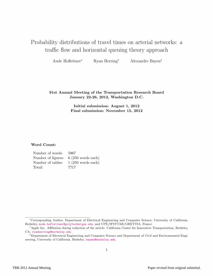
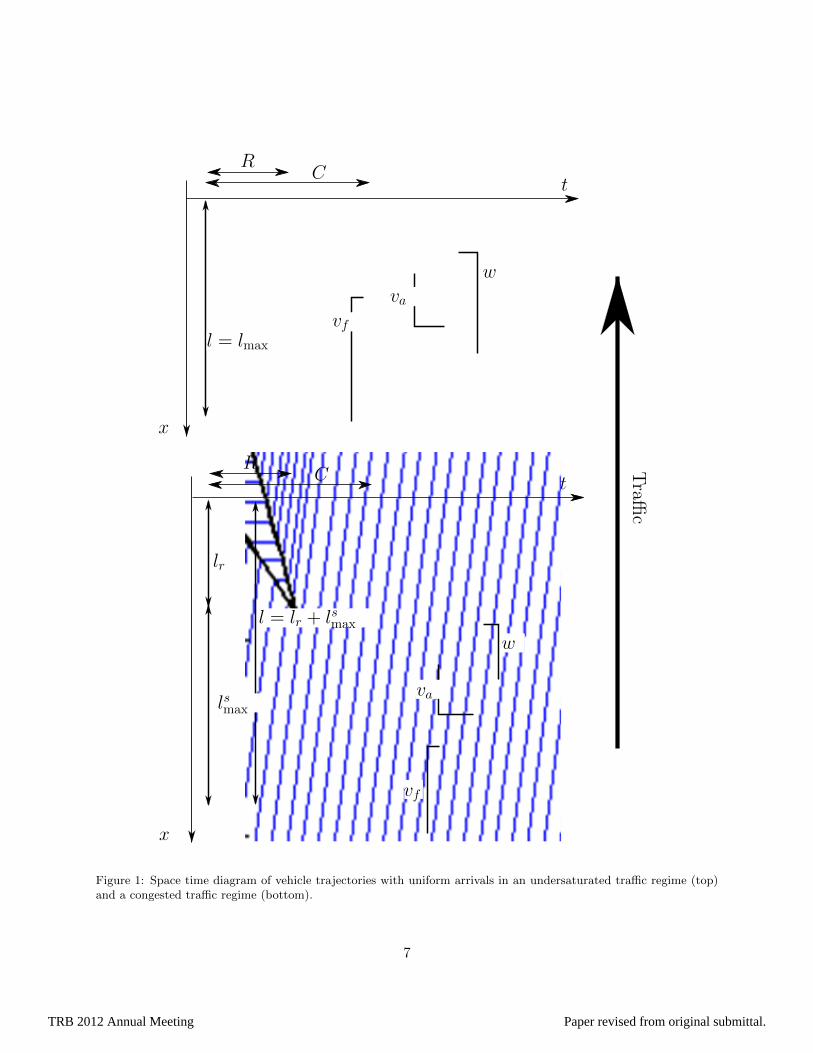
remaining queue when the light switches from green to red. Figure 1 illustrates these two regimes118

under the assumptions made in Section 2.2. The speed of formation and dissolution of the queue119

are respectively called va and w. Their expression is derived from the Rankine-Hugoniot [15]120

jump conditions and given by121

va =ρavf

ρmax − ρaand w =

ρcvfρmax − ρc

. (2)

Undersaturated regime. In this regime, the queue fully dissipates within the green time.122

This queue is called the triangular queue (from its triangular shape on the space-time diagram123

of trajectories). It is defined as the spatio-temporal region where vehicles are stopped on the124

link. Its length is called the maximum queue length, denoted lmax, which can also be computed125

from traffic theory:126

lmax = Rwvaw − va

= Rvfρmax

ρcρaρc − ρa

. (3)

Congested regime. In this regime, there exists a part of the queue downstream of the tri-127

angular queue called the remaining queue with length lr corresponding to vehicles which must128

stop multiple times before going through the intersection.129

All notations introduced up to here are illustrated for both regimes in Figure 1.130

131

Stationarity of the two regimes. Assumption 2 made earlier implies the periodicity of these132

queue evolutions. In particular, there is not a consistent increase or decrease in the length of the133

5


queue for the duration of the time interval. This assumes that the congested regime is exactly134

at saturation: the numbers of vehicles entering and exiting the link during a cycle are equal.135

At saturation, the arrival density is ρsa = C−RC ρc. The triangular queue length at saturation is136

computed by replacing ρa = ρsa in equation (3) or by noticing that the number of vehicles that137

stop in the queue (lsmaxρmax) is equal to the number of vehicles that exit the link in the duration138

of a cycle ((C −R)vfρc):139

lsmax = vfρc(C −R)/ρmax (4)

Note that saturation is an idealized notion that we assume valid for small time intervals. In140

the following, x is used to denote the distance from a location on a link to the downstream141

intersection.142

The undersaturated and congested regimes are labeled u and c respectively. A probabilistic143

model based on the assumptions formulated in this section provides the probability distribution144

function pdf of delays δx1,x2and travel times yx1,x2

between two locations x1 and x2 on a link of145

the network. They are denoted h(δx1,x2) (Section 3) and g(yx1,x2

) (Section 4) respectively. These146

pdf are parameterized by the traffic parameters: the free flow pace pf with pdf ϕp (parameterized147

by θp), the cycle time C, the red time R, the queue length at saturation lsmax and the queue148

length l. Note that l = lmax, length of the triangular queue in the undersaturated regime and149

l = lsmax + lr, sum of the length of the triangular queue at saturation and the remaining queue in150

the congested regime. This set of variables is sufficient to characterize the distribution of travel151

times resulting from the modeling assumptions.152

3 Modeling the probability distribution of stopping time153

The delay experienced by vehicles traveling on arterial networks is conditioned on two factors.154

First, the traffic conditions dictate the state of traffic experienced by all vehicles entering the155

link. Second, the time (in relation to the beginning of the signal’s cycle) at which each vehicle156

enters a link determines how much delay will be experienced in the queue due to the presence of157

the traffic signal. Under similar traffic conditions, drivers experience different delays depending158

on their arrival time. Using the assumption that the arrival density (and thus the arrival rate) is159

constant, arrival times are uniformly distributed on the duration of the light cycle. This allows160

us to derive the analytical expression, hs(δx1,x2), s ∈ {u, c} of the pdf of stopping time δx1,x2

161

between locations x1 and x2.162

In this work, we assume that we receive travel time measurements from vehicles traveling163

on the network. The vehicles are sampled uniformly in time, as is commonly done with fleets,164

and they send tuples of the form (x1, t1, x2, t2) where x1 is the location of the vehicle at t1, x2165

is the position of the vehicle at t2 and t2− t1 represents the sampling interval (usually constant166

from one measurement to another). This is representative of fleets which typically send data167

every minute in urban networks. We consider the tuples sent by the vehicles as independent.168

For example, we assume that the sampling strategy is such that we cannot reconstruct the169

trajectories of vehicles from the tuples (e.g. at each sampling time, the vehicles send tuples170

with a defined probability).171

3.1 Pdf of stopping time in the undersaturated regime172

In the undersaturated regime, we call ηux1,x2the fraction of the vehicles entering the link during173

a cycle that experience a delay between x1 and x2. The remaining vehicles entering the link in174

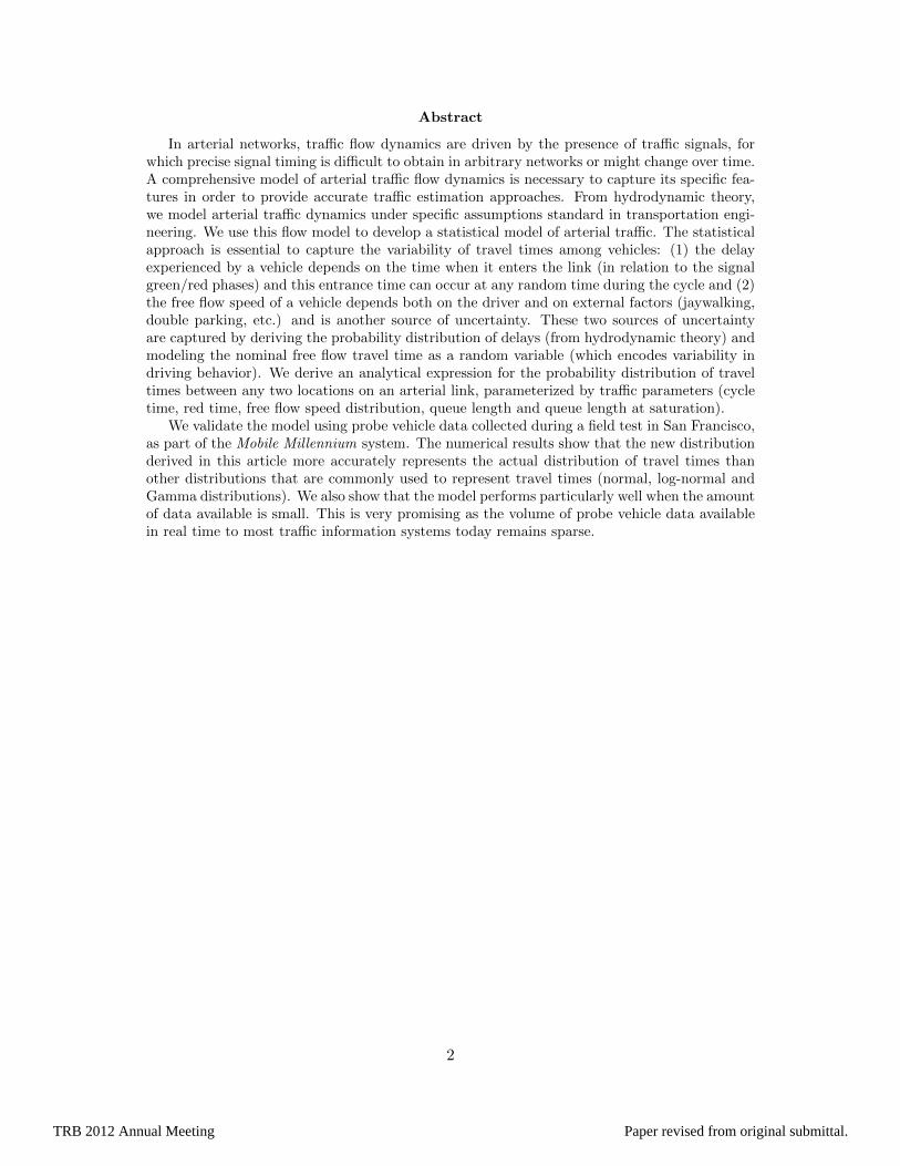
a cycle travel from x1 to x2 without experiencing any delay. The proportion ηux1,x2is computed175

as the ratio of vehicles joining the queue between x1 and x2 over the total number of vehicles en-176

tering the link in one cycle (Figure 2). The number of vehicles joining the queue between x1 and177

x2 is the number of vehicles stopped between x1 and x2:(min(lmax, x1)−min(lmax, x2)

)ρmax.178

The number of vehicles entering the link is vfCρa. The proportion of vehicles delayed between179

6


RC

RC T

raffic

t

x

t

x

l = lmax

w

vf

va

l = lr + lsmax

lr

w

vf

valsmax

Figure 1: Space time diagram of vehicle trajectories with uniform arrivals in an undersaturated traffic regime (top)and a congested traffic regime (bottom).

7


Traffi

c

t

x

x2

x1

x

(x1 − x2)ρmax

δu(x2)

δu(x1)

Cvfρa

Figure 2: The proportion of delayed vehicles ηux1,x2is the ratio between the number of vehicles joining the queue

between x1 and x2 over the total number of vehicles entering the link in one cycle. The trajectories highlighted inpurple represent the trajectories of vehicles delayed between x1 and x2.

x1 and x2 is thus ηux1,x2= (min(x1, lmax)−min(x2, lmax)) ρmax

vfCρa. Multiplying the nominator and180

denominator by lmax, using equation (3) to eliminate ρa and equation (4), we have the expression181

of ηux1,x2in terms of the model parameters R, C and lsmax and the state variable l = lmax:182

ηux1,x2=

min(x1, lmax)−min(x2, lmax)

lmax

(R

C+

(1− R

C

)lmax

lsmax

).

The first factor scales the proportion of stopping vehicles as a function of the measurement183

locations. The second factor represents the proportion of stopping vehicles if x1 is upstream of184

the queue and x2 is at the intersection. As the queue length lmax tends to zero, the fraction185

of stopping vehicles tends to R/C. When the queue length increases, the fraction of stopping186

vehicles increases linearly until it reaches one at saturation (lmax = lsmax).187

The stopping time experienced when stopping at x is denoted by δu(x) for the undersaturatedregime. Because the arrival of vehicles is homogenous, the delay δu(x) increases linearly withx. At the intersection (x = 0), the delay is maximal and equals the duration of the red lightR. At the end of the queue (x = lmax) and upstream of the queue (x ≥ lmax), the delay is null.Thus the expression of δu(x) is as follows:

δu(x) = R

(1− min(x, lmax)

lmax

).

Given that the arrival of vehicles is uniform in time, the distribution of the location where188

the vehicles reach the queue between x1 and x2 is uniform in space. For vehicles reaching the189

queue between x1 and x2, the probability to experience a delay between locations x1 and x2 is190

uniform. The uniform distribution has support [δu(x1), δu(x2)], corresponding to the minimum191

and maximum delay between x1 and x2.192

8


The stopping time of vehicles between x1 and x2 is a random variable with a mixture distri-bution with two components. The first component represents the vehicles that do not experienceany stopping time between x1 and x2 (mass distribution in 0), the second component representsthe vehicles reaching the queue between x1 and x2 (uniform distribution on [δu(x1), δu(x2)]).We note 1A the indicator function of set A,

1A(x) =

{1 if x ∈ A0 if x /∈ A

The Dirac distribution centered in a, used to represent a mass probability is denoted Dir{a}(·).193

The pdf of total delay between x1 and x2 (Figure 3, left) reads:

ht(δx1,x2) = (1− ηux1,x2

)Dir{0}(δx1,x2) +

ηux1,x2

δu(x2)− δu(x1)1[δu(x1),δu(x2)](δx1,x2

)

The cumulative distribution function of total delay Ht(·) reads:

Ht(δx1,x2) =

0 if δx1,x2 < 0(1− ηux1,x2

) if δx1,x2∈ [0, δu(x1)]

(1− ηux1,x2) + ηux1,x2

δx1,x2−δu(x1)

δu(x2)−δu(x1) if δx1,x2∈ [δu(x1), δu(x2)]

1 if δx1,x2> δu(x2)

3.2 Pdf of stopping time in the congested regime194

For the congested regime, as for the undersaturated regime, the pdf of stopping time is computedby deriving the delay experienced between x1 and x2 for each arrival time in a cycle. The distancetraveled by vehicles in the queue in the duration of a light cycle is lsmax. We call ns the maximumnumber of stops experienced by the vehicles in the remaining queue between the locations x1

and x2:

ns =

⌈min(x1, lr)−min(x2, lr)

lsmax

⌉.

In this article, we do not model specifically queue spill-over to upstream links. However, this195

vital component is indirectly taken into account by the flexibility of a statistical model. Indeed, a196

queue spill-over has the effect to reduce the flow that can exit the upstream links and change the197

behavior on these links accordingly. The statistical model will automatically learn from the data198

the new parameters of the dynamics. The delay experienced at location x when reaching the199

triangular queue at x is readily derived from the expression of the delay in the undersaturated200

regime, noticing that the delay for x o, the remaining queue is R:201

δc(x) =

R if x ≤ lr

Rlr+lsmax−x

lsmaxif x ∈ [lr, lr + lsmax]

0 if x ≥ lr + lsmax

The details of the derivation are given in [22] (Section 4.3 and Appendix A). We summarize202

the derivations, classified depending on the location of the positions x1 and x2 with respect to the203

remaining (lr) and saturation (lsmax) queue lengths. The analytical results are also summarized204

in Table 1.205

1. x1 Upstream – x2 Remaining (x1 ≥ lr + lsmax, x2 ≤ lr): We define the critical location xc byxc = x2 +nsl

smax. Vehicles reaching the triangular queue upstream (resp. downstream) of xc

stop ns (resp. ns−1) times in the remaining queue on the road segment [x1, x2]. The vehicles

9


experience a delay uniformly distributed on [δmin, δmax] with δmin = (ns − 1)R + δc(xc) andδmax = nsR+ δc(xc) = δmin +R. The pdf of stopping time reads:

ht(δx1,x2) =

1

δmax − δmin1[δmin,δmax](δx1,x2

),δmin = δc(xc) + (ns − 1)R,δmax = δc(xc) + nsR

.

2. x1 Triangular – x2 Triangular (x1, x2 ≥ lr): Given that the path is upstream of the remainingqueue, this case is similar to the undersaturated regime, where derivations are updated toaccount for the fact that the triangular queue starts at x = lr. We adapt the notation fromSection 3.1 and denote by ηcx1,x2

the fraction of the vehicles entering the link in a cycle thatexperience delay between locations x1 and x2.

ηcx1,x2=

min(x1 − lr, lsmax)−min(x2 − lr, lsmax)

lsmax

.

This delay is uniformly distributed on [δc(x1), δc(x2)]. The remainder do not stop betweenx1 and x2. The pdf of stopping time reads:

ht(δx1,x2) = (1− ηcx1,x2)Dir{0}(δx1,x2) +

ηcx1,x2

δc(x2)− δc(x1)1[δc(x1),δc(x2)](δx1,x2

).

3. x1 Remaining – x2 Remaining (x1, x2 ≤ lr): We define the critical location xc by xc =x2 + (ns − 1)lsmax. The vehicles reaching the queue between x1 and xc stop ns times in theremaining queue between x1 and x2, their stopping time is nsR. The reminder of the vehiclesstop ns − 1 times in the remaining queue and their stopping time is (ns − 1)R. The pdf ofstopping time reads:

ht(δx1,x2) =

x1 − xclsmax

Dir{nsR}(δx1,x2) +

(1− x1 − xc

lsmax

)Dir{(ns−1)R}(δx1,x2

).

4. x1 Triangular – x2 Remaining (x1 ∈ [lr, lr + lsmax], x2 ≤ lr): We define the critical location206

xc by xc = x2 + nslsmax.207

� If x1 ≥ xc, a fraction (x1 − xc)/lsmax of the vehicles entering the link in a cycle join the208

triangular queue between x1 and xc. They stop once in the triangular queue and ns times209

in the remaining queue. Among these vehicles, the stopping time is uniformly distributed210

on [δc(x1)+nsR, δc(xc)+nsR]. A fraction (xc−lr)/lsmax of the vehicles entering the link in211

a cycle join the triangular queue between xc and lsmax. Among these vehicles, the stopping212

time is uniformly distributed on [δc(xc) + (ns − 1)R, nsR]. The remainder of the vehicles213

reach the remaining queue between lr and x1 − lsmax and their stopping time is nsR. The214

pdf of stopping time reads:215

ht(δx1,x2) =x1 − xclsmax

1[δc(x1)+nsR, δc(xc)+nsR](δx1,x2)

δc(xc)− δc(x1)stop between x1 and xc

+xc − lrlsmax

1[δc(xc)+(ns−1)R,nsR](δx1,x2)

R− δc(xc)stop between xc and lr

+

(1− x1 − lr

lsmax

)Dir{nsR}(δx1,x2

). stop between lr and x1 − lsmax

� If x1 ≤ xc, a fraction (x1 − lr)/lsmax of the vehicles entering the link in a cycle join the216

triangular queue between x1 and lr. They stop once in the triangular queue and ns−1 times217

in the remaining queue. Among these vehicles, the stopping time is uniformly distributed218

on [δc(x1) + (ns− 1)R, nsR]. A fraction 1− (xc− lr)/lsmax of the vehicles entering the link219

10


in a cycle join the remaining queue between lr and xc − lsmax. The stopping time of these220

vehicles is nsR. The remainder of the vehicles experiences a stopping time of (ns − 1)R.221

The pdf of stopping time reads:222

ht(δx1,x2) =

x1 − lrlsmax

1[δc(x1)+(ns−1)R,nsR](δx1,x2)

R− δc(x1)stop between x1 and lr

+

(1− xc − lr

lsmax

)Dir{nsR}(δx1,x2

) stop between lr and xc − lsmax

+xc − x1

lsmax

Dir{(ns−1)R}(δx1,x2). stop between xc − lsmax and x1 − lsmax

4 Probability distributions of travel times and estimation223

from sparsely sampled probe vehicles224

4.1 Travel time distributions225

Along the path between x1 and x2, the travel time yx1,x2is a random variable, written as the226

sum of two independent random variables: the delay δx1,x2 experienced between x1 and x2 and227

the free flow travel time of the vehicles yf ; x1,x2 . The free flow travel time is proportional to228

the distance of the path and the free flow pace pf such that yf ; x1,x2= pf (x1 − x2). We have229

yx1,x2= δx1,x2

+ yf ; x1,x2.230

We model the differences in traffic behavior by considering the free flow pace pf as a random231

variable with distribution ϕp and domain of definition Dϕp . For convenience, we define the232

extension of ϕ as being zero on R\Dϕp (the complement of the domain of definition), which do233

not change the distribution of the random variable pf . With a slight abuse of notation, we still234

call this extension ϕ.235

Using a linear change of variables, we derive the probability distribution ϕyx1,x2of free flow236

travel time yf ; x1,x2 between x1 and x2:237

pf ∼ ϕp(pf )⇒ ϕyx1,x2(yf ; x1,x2

) = ϕp(yf ; x1,x2

x1 − x2

)1

x1 − x2

To derive the pdf of travel times we use the following fact:238

Fact 1 (Sum of independent random variables). If X and Y are two independent random239

variables with respective pdf fX and fY , then the pdf fZ of the random variable Z = X + Y is240

given by the convolution product of fX and fY , denoted fZ(z) = (fX ∗ fY ) (z) and defined as241

fZ(z) =∫RfX(t)fY (z − t) dt.242

This classical result in probability is derived by computing the conditional pdf of Z given X243

and then integrating over the values of X according to the total probability law.244

For each regime s ∈ {u, c}, the probability distribution of travel times reads:

gs(yx1,x2) =

(hs ∗ ϕyx1,x2

)(yx1,x2

).

We derive the general expression of the travel time distributions when vehicles experience a245

delay with mass probability in ∆ and when vehicles experience a delay with uniform distribution246

on [δmin, δmax]. These expressions enable the computation of the pdf of travel times using the247

linearity of the convolution operator.248

Travel time distribution when the delay has a mass probability in ∆:249

11


Case Trajectories Weight Dist. Support

Case 1x1 ≥ lr + lsmax,x2 ≤ lr,xc = x2 + nsl

smax

All 1 Unif.[(ns − 1)R+ δc(xc),nsR+ δc(xc)]

Case 2x1 ≥ lr,x2 ≥ lr

No stop between x1 and x2P(s̄x1 , s̄x2)×(1− ηcx1,x2

)Mass {0}

Reach the (triangular)queue between x1 and x2

P(s̄x1 , s̄x2)×ηcx1,x2

Unif. [δc(x2), δc(x1)]

Case 3x1 ≤ lr,x2 ≤ lr,xc = x2 + (ns − 1)lsmax

Reach the (remaining)queue between x1 and xc

P(s̄x1 , s̄x2)×x1 − xclsmax

Mass {nsR}

Reach the (remaining)queue between xc andx1 − lsmax

P(s̄x1 , s̄x2)×xc − x1 + lsmax

lsmax

Mass {(ns − 1)R}

Case 4ax1 ∈ [lr, lr + lsmax],x2 ≤ lr,xc = x2 + nsl

smax,

xc ≤ x1

Reach the (triangular)queue between x1 and xc

P(s̄x1 , s̄x2)×x1 − xclsmax

Unif.[nsR+ δc(x1),nsR+ δc(xc)]

Reach the (triangular)queue between xc and lr

P(s̄x1 , s̄x2)×xc − lrlsmax

Unif.[(ns − 1)R+ δc(xc),nsR]

Reach the (remaining)queue between lr andx1 − lsmax

P(s̄x1 , s̄x2)×lr − x1 + lsmax

lsmax

Mass {nsR}

Case 4bx1 ∈ [lr, lr + lsmax],x2 ≤ lr,xc = x2 + nsl

smax,

xc ≥ x1

Reach the (triangular)queue between x1 and lr

P(s̄x1 , s̄x2)×x1 − lrlsmax

Unif.[(ns − 1)R+ δc(x1),nsR]

Reach the (remaining)queue between lr andxc − lsmax

P(s̄x1 , s̄x2)×lr − xc + lsmax

lsmax

Mass {nsR}

Reach the (remaining)queue between xc − lsmax

and x1 − lsmax

P(s̄x1 , s̄x2)×xc − x1lsmax

Mass {(ns − 1)R}

Table 1: The pdf of measured delay is a mixture distribution. The different components and their associated weightdepend on the location of stops of the vehicles with respect to the queue length and sampling locations.

12


The stopping time is ∆. This corresponds to trajectories with ns stops (ns ≥ 0) in the250

remaining queue. This includes the non stopping vehicle in the undersaturated regime, when251

the remaining queue has length zero. The travel time distribution is derived as252

g(yx1,x2) =

(Dir{∆} ∗ ϕyx1,x2

)(yx1,x2

)

= ϕyx1,x2(yx1,x2

−∆). (5)

Travel time distribution when the delay is uniformly distributed on [δmin, δmax]:253

Vehicles experience a uniform delay between a minimum and maximum delay respectively254

denoted δmin and δmax. The probability of observing a travel time yx1,x2is given by255

g(yx1,x2) =

1

δmax − δmin

∫ +∞

−∞1[δmin,δmax](yx1,x2

− z) ϕyx1,x2(z) dz. (6)

The integrand is not null if and only if yx1,x2 − z ∈ [δmin, δmax], i.e. if and only if z ∈256

[yx1,x2 − δmax, yx1,x2 − δmin]. Since ϕyx1,x2(z) is equal to zero for z ∈ R \ Dϕ, the integrand is257

not null if and only if z ∈ [yx1,x2− δmax, yx1,x2

− δmin]⋂Dϕ.258

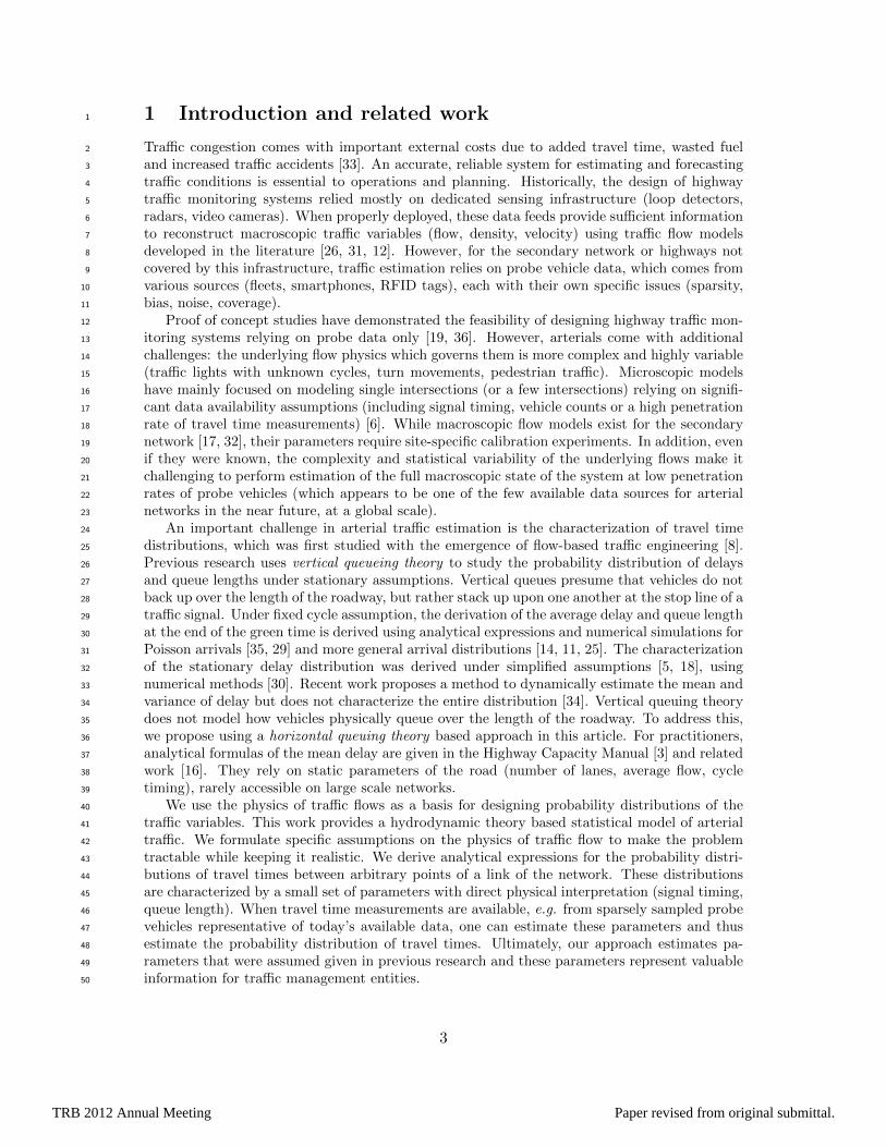
259

As an illustration, we derive the probability distribution of travel times on a partial link in the260

undersaturated regime, for a pace distribution with support on R+. In this article, we denote261

by support the set of points where the function is not zero. We write the delay distribution262

as a mixture of mass probabilities and uniform distributions with two components. The first263

component, with weight 1 − ηux1,x2, represents the delay distribution of the vehicles which do264

not stop between x1 and x2. It is a mass distribution in 0. The second component, with weight265

ηux1,x2, represents the delay distribution of the vehicles who do stop between x1 and x2. It is266

a uniform distribution with support [δu(x1), δu(x2)]. The probability distribution of delay is267

illustrated Figure 3 (left) with different line styles for the two components. We use the linearity268

of the convolution to convolve each component of the mixture with the probability distribution269

of free flow travel times ϕyx1,x2. The pdf of travel times are computed according to (5) and (6) for270

the non-stopping and the stopping vehicles respectively and are illustrated Figure 3 (center). We271

sum the pdf of travel times of the non-stopping and the stopping vehicles with their respective272

weights (1 − ηux1,x2and ηux1,x2

) to obtain the pdf of travel times between locations x1 and x2273

for all the vehicles entering the link in a cycle (Figure 3, right). The probability distribution of274

travel times reads:275

gu(yx1,x2) =

0 if yx1,x2≤ 0,

(1− ηux1,x2)ϕyx1,x2

(yx1,x2) if yx1,x2

∈ [0, δu(x1)],(1− ηux1,x2

)ϕyx1,x2(yx1,x2)

+ηux1,x2

δu(x2)−δu(x1)

yL,0−δu(x1)∫0

ϕyx1,x2(z) dz

if yx1,x2 ∈ [δu(x1), δu(x2)],

(1− ηux1,x2

)ϕyx1,x2(yx1,x2)

+ηux1,x2

δu(x2)−δu(x1)

yL,0−δu(x1)∫yL,0−δu(x2)

ϕyx1,x2(z) dz

if yx1,x2≥ δu(x2).

The derivations are similar in the congested regime: we convolve each component of the276

stopping time distribution with the pdf of free flow travel times ϕyx1,x2. We recall that for the277

different cases described in Section 3.2, the delay is a mixture of mass probabilities and uniform278

distributions and thus either equation (5) or (6) is used on each component.279

13


0 10 20 300

0.05

0.1

0.15

0.2

0.25

0.3

Delay (s)

pd

fPdf of delays

0 20 40 600

0.01

0.02

0.03

0.04

0.05

Travel time (s)p

df

Components of the pdf of travel times

Component 1: not stoppingComponent 2: stopping

0 20 40 600

0.01

0.02

0.03

0.04

0.05

Travel time (s)

pd

f

Pdf of travel times

Sum: travel time distribution

Figure 3: Probability distributions of travel times between arbitrary locations in the undersaturated regime. Thefigure represents the pdf of travel times between x1 and x2 where both x1 and x2 are in the triangular queue, withδu(x1) = 10s and δu(x2) = 30s and ηux1,x2

= 0.7. The free flow travel time between x1 and x2 is a random variablewith Gamma distribution. The mean free flow travel time is 10 seconds and the standard deviation is 3s.

For example, the probability distribution of link travel times (Case 1, x1 = L length of the280

link, x2 = 0) is computed via equation (6) and reads281

gc(yL,0) =

0 if yL,0 ≤ δmin,

1δmax−δmin

∫ yL,0−δmin

0ϕyL,0(z)dz if yL,0 ∈ [δmin, δmax],

1δmax−δmin

∫ yL,0−δmin

yL,0−δmaxϕyL,0(z) dz if yL,0 ≥ δmax.

with δmin = δc(nslsmax) + (ns − 1)R, δmax = δc(nsl

smax) + nsR and ns =

⌈lrlsmax

⌉.282

4.2 Learning traffic conditions from sparsely sampled probe vehicles283

From traffic flow theory, we derived a probability distribution of travel times between arbitrary284

locations on an arterial link. These distributions are parameterized by the network parameters285

(average red time R, average cycle time C, driving behavior θp and saturation queue length286

lsmax) and the level of congestion represented by the queue length lmax. As probe vehicles report287

their location periodically in time, the duration between two successive location reports x1 and288

x2 represents a measurement of the travel time of the vehicle on its path from x1 to x2. We289

use these travel time observations from probe vehicles to learn the parameters of the travel time290

distributions.291

Common sampling rates for probe vehicles are around one minute and probe vehicles typically292

traverse several links between successive location reports. It is possible to optimally decompose293

the path travel time to estimate the travel time spent on each link of the path [20]. In this article,294

we assume that this decomposition has already been achieved and we focus on the estimation295

of the pdf of travel times. Since probe vehicles may report their location at any point x1 and296

x2, they provide partial link travel time measurements that allow for the estimation of the297

independent parameters of each link: the red time R, the queue length lmax, the fraction of298

stopping vehicles on the link among the vehicles entering the link in one cycle ηuL,0 and the299

driving behavior θp. The estimation of the parameters of link i is done by maximizing the300

likelihood (or more conveniently the log-likelihood) of the (partial) link travel times of this link301

with respect to these parameters. Note that the parameters of the travel time distribution (Ri,302

14


ηuL,0, li and θip) do not depend on the locations x1 and x2 of measurement j. In particular, we303

learn the travel time distributions using travel time measurements which span different portions304

of the link, i.e. the locations x1 and x2 depend on the index of the measurement (j), even305

though we do not explicit this dependency for notational simplicity. Let (yjx1,x2)j=1:Ji represent306

the set of (partial link) travel times allocated to link i. The estimation problem is given by:307

minimizeRi,ηuL,0,l

i,θip

Ji∑j=1

− ln(gi(yjx1,x2)) (7)

s.t. ηuL,0 ∈ [0, 1], li ∈ [0, Li].

Additional constraints and bounds may be added to limit the feasible set to physically308

acceptable values of the parameters and improve the estimation when little data is available.309

The optimization problem (7) is not convex but it is a small scale optimization problem (feasible310

set of dimension five). Numerous optimization techniques can be used to solve this problem311

including global optimization algorithms [23, 37]. Moreover, since the parameters represent312

physical parameters, they can be bounded to limit the feasible set to a compact set (of dimension313

five). It is thus possible to do a grid search. The grid search algorithm defines a grid on the314

bounded feasible set and evaluates the objective function for each set of parameters defined by315

the grid. We keep the B best set of parameters, associated with the lowest values of the objective316

function and perform a first or a second order optimization algorithm [10] from this best set of317

parameters. In the implementation of the algorithm used to produce the results of Section 5,318

we set B = 4 and used the active-set algorithm in the Matlab [1] optimization toolbox, which319

is a second order optimization algorithm based on Sequential Quadratic Programming [9].320

5 Numerical experiments and results321

The model presented in this article relies on assumptions on the dynamics of traffic flows on322

each link of the network to derive probability distributions of travel times. The goal of this323

section is to show numerically that these travel time distributions, derived from the physics of324

traffic flows, represent the empirical distribution of travel times more accurately than classical325

distributions such as normal, log-normal or Gamma distributions.326

We consider four classes of distributions: the traffic distribution derived in this article, the327

normal distribution, the log-normal distribution and the Gamma distribution. For each class328

of distributions, we test the hypothesis that link travel times are distributed according to this329

distribution (the complementary hypothesis is that the travel times are not distributed according330

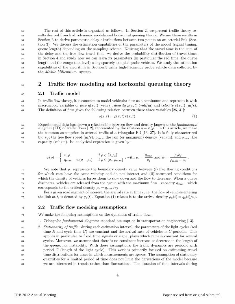
to this distribution). We use data collected during a field experiment from the 29th of June331

to the 1st of July 2010 as part of the Mobile Millennium project [2, 7]. Twenty drivers, each332

carrying a GPS device, drove for 3 hours (3:15pm to 6:15pm) around two distinct loops in San333

Francisco. The first loop was 1.89 miles long and the second one 2.31 miles long. The GPS334

devices recorded the location of the vehicles every second and provided detailed information on335

the trajectories of the drivers. From this detailed data, we extract link travel times.336

For each link of the network, we compute the maximum likelihood estimates of the dis-337

tribution parameters for each class of distributions. This learning of distribution parameters338

is performed using a fraction of the link travel times collected by the drivers. We vary the339

percentage of available data used for the training of the distributions to study the influence of340

the amount of data required to learn the parameters accurately. For each class of distribution,341

we test the hypothesis H0: the link travel times are distributed according to the distribution on342

the validation link travel times using the Kolmogorov-Smirnov test [28], also referred to as K-S343

test. The K-S test is a standard non-parametric test to state whether samples are distributed344

15


1st loop

2nd loop

Figure 4: Experimental set-up of the field experiment representing the two distinct loops in downtown San Francisco,CA.

according to an hypothetical distribution (in opposition to other tests like the T-test that tests345

uniquely the mean, or the chi-squared test that assumes that the data is normally distributed).346

The test is based on the K-S statistics which is computed as the maximum difference between347

the empirical and the hypothetical cumulative distributions. The test provides a p-value which348

informs us on the goodness of the fit. Low p-values indicate that the data does not follow the349

hypothetical distribution. For each hypothetical distribution, Figure 5 (left) shows the average350

p-value of the links of the network as the percentage of training data increases. The hypothesis351

H0 is rejected for p-values inferior to the significance level α. The significance level α corre-352

sponds to the percentage of Type-I error allowed by the test (rejecting the null hypothesis when353

it is actually true). Figure 5 (right) shows the evolution of the percentage of links that passes the354

K-S test at significance level α = 0.1. Both figures show that the traffic distribution represents355

a better fit of the travel time distributions than any of the other distributions tested in this356

article. We notice that the relative superiority of the traffic model is more significant when little357

data is available. This may be a sign of the robustness of the model when little data is available358

(because of the intrinsic structure of the distributions representing the physical model). This359

is precisely the goal of the algorithm (and model), which was specifically created to handle low360

volumes of probe data. We also notice that the log-normal model performs well compared to361

the normal or the Gamma distribution.362

We analyze the differences of the traffic and the log-normal by studying the empirical dis-363

tribution of travel times. Figure 6 (left) shows the hypothetical and empirical distribution of364

travel times. The traffic distribution captures the specific characteristics of traffic dynamics.365

We can see a peak in the distribution representing the vehicles that do not stop on the link366

and travel at their free flow speed. For higher travel times, the distribution is approximately367

uniform, representing the vehicles that are delayed on the link, between a minimum delay (0)368

and a maximum delay (the duration of the red time). As for the log-normal distribution, it369

cannot capture these specifics of the travel time distribution and the parameters are harder to370

interpret.371

Due to light synchronization, some links have arrivals with platoons, and thus do not follow372

the hypothesis of constant arrivals. On these links, delays are not uniformly distributed among373

16


30 40 50 60 70 80 90 100

0.1

0.15

0.2

0.25

Percentage of training data

Ave

rag

e p

val

ue

TrafficNormalLog normalGamma

30 40 50 60 70 80 90 10020

25

30

35

40

45

50

55

Percentage of training data

Per

cen

tag

e o

f lin

ksw

ith

p v

alu

e ab

ove

0.1

Figure 5: Goodness of fit of the model depending on the percentage of training data used to learn the parameters.(Left) Average p-value of the links of the network for the different hypothetical distributions (traffic, normal, log-normal and Gamma). (Right) Percentage of links that pass the KS test with a significance level α = 0.1.

Link 1

20 40 60 80 1000

0.01

0.02

0.03

0.04

0.05

Travel time (s)

pd

f

Histogram of the data (50 points)Estimated traffic pdfEstimated Log normal pdf

20 40 60 80 1000

0.5

1

1.5

Travel time (s)

cdf

Estimated traffic cdfEstimated Log normal cdfEmpirical cdf

Link 2

10 20 30 40 50 60 70 80 900

0.02

0.04

0.06

Travel time (s)

pd

f

Histogram of the data (28 points)Estimated traffic pdfEstimated Log normal pdf

10 20 30 40 50 60 70 80 900

0.5

1

1.5

Travel time (s)

cdf

Estimated traffic cdfEstimated Log normal cdfEmpirical cdf

Figure 6: Comparison of the traffic and the log-normal distributions with the empirical distribution of travel timeson two links of the network. The figure represents both the pdf and the cdf of the traffic (solid blue line) and log-normal (dashed red line) distributions. The histograms on the top figures represent interval counts of the probe traveltimes, normalized so that the area of the histogram sums to one. The cumulated histograms (bottom figures) are thecumulated distributions of the histograms. The black line with circles represents the empirical cumulative distribution(Kaplan-Meier estimate [24]) of the travel times collected by the probes. (Left, link 1) Both distributions capturethe long tail of the distribution but only the traffic distribution is able to represent the peak in the pdf due to thenon stopping vehicles and to estimate accurately the maximum delay. (Right, link 2) On this link, we notice veryfew travel times between 35 and 50 seconds, likely due to important synchronization with the upstream link. Noneof the traffic or log-normal distribution is able to capture this. However, the traffic distribution models accuratelythe peak due to the non stopping vehicles and estimate the maximum delay.

17


the stopping vehicles and the derivations of the queuing model have to be adapted [4]. Basically,374

the delay function δr(x) (r ∈ {u, c}, see Section 3) is piecewise linear and the derivations of the375

statistical distributions must be updated accordingly, adding parameters to the model. Figure 6376

(right) represents the empirical and hypothetical distribution of travel times for a link with377

platoon arrivals. We can see that there are very few vehicles with a travel time between 30 and378

50 seconds, representing a time interval during which there is very few arrivals on the links,379

likely when the upstream signal is red. We notice that the log-normal distribution does not380

capture this characteristics of the distribution either. Moreover, the traffic model provides an381

estimation of the red time, the free flow speed and the fraction of stopping vehicles (representing382

congestion) which is important information for traffic management and operations.383

6 Conclusion384

In this article, we derived a parametric probability distribution of travel times between arbitrary385

locations on an arterial link. This probability distribution is derived from hydrodynamic theory386

and represents the dynamics of traffic flow on arterial links. In particular, it captures the delay of387

vehicles due to the presence of a queue that forms and dissipates periodically because of the traffic388

signal. These distributions are parameterized by physical parameters: the red time, the cycle389

time, the parameters of the free flow pace, the queue length and the saturation queue length.390

Depending on the data available, these parameters may not be estimated independently, but we391

can always retrieve the duration of the red time, the level of congestion and the parameters of392

the free flow pace . The queue length can also be estimated from probe vehicles reporting their393

location at any location on the link.394

The goodness of fit of the distributions was tested on probe data collected during a field395

test in San Francisco. The numerical results show the superiority of the traffic distribution396

to represent the distribution of travel times compared to “classic” distributions (normal, nog-397

normal and Gamma distributions), commonly used to represent the distribution of travel times.398

The traffic distribution performs particularly well (in comparison with the other distributions)399

when little data is available.400

The numerical analysis shows that the uniform arrivals is the most restrictive assumption on401

which this work is based, as it does not take into account signal synchronization. We are cur-402

rently working on a generalization of the proposed approach in which vehicles arrive in platoons403

of homogeneous density. Note that this generalization does not invalidate the methodology pre-404

sented in this article. In particular, the probability distribution of stopping times will remain a405

mixture of discrete mass probabilities and uniform distributions.406

The probability distribution of travel times are finite mixture distributions [20]. Each com-407

ponent of the mixture corresponds to a type of delay: stopping or not stopping for the under-408

saturated regime or depending on the location of the vehicle (Table 1) in the congested regime.409

The estimation of transition probabilities representing the probability of a type of delay on a410

link given the type of delay on the upstream link would allow to compute route travel time411

distributions with a Markov chain approach.412

Acknowledgements413

The authors wish to thank Pieter Abbeel from UC Berkeley for his valuable contribution and414

feedback on the model presented in this article. We thank the California Center for Innovative415

Transportation (CCIT) staff for their contributions to develop, build, and deploy the system416

infrastructure of Mobile Millennium on which this article relies and for their help in the logistical417

planning of the field test described in this article. This research was supported by the Federal418

and California DOTs, Nokia, Center for Future Urban Transport at UC Berkeley (a Volvo419

18


International Center of Excellence) and the Center for Information Technology Research in the420

Interest of Society (CITRIS).421

References422

[1] MATLAB. http://mathworks.com.423

[2] The Mobile Millennium Project. http://traffic.berkeley.edu.424

[3] Highway Capacity Manual. TRB, National Research Council, Washington, D.C., 2000.425

[4] R. E. Allsop. An analysis of delays to vehicle platoons at traffic signals. In Procedings of426

the fourth international symposium on the Theory of Traffic Flow, University of Karlsruhe,427

Germany, 1968.428

[5] R. E. Allsop. Delay at fixed time traffic signals-I: Theoretical analysis. Transportation429

Science, 6:280–285, 1972.430

[6] X. Ban, R. Herring, P. Hao, and A. Bayen. Delay pattern estimation for signalized in-431

tersections using sampled travel times. In Proceedings of the 88th Annual Meeting of the432

Transportation Research Board, Washington, D.C., January 2009.433

[7] A. Bayen, J. Butler, and A. Patire et al. Mobile Millennium final report. Technical434

report, University of California, Berkeley, CCIT Research Report UCB-ITS-CWP-2011-435

6, To appear in 2011.436

[8] D. S. Berry and D. M. Belmont. Distribution of vehicle speeds and travel times. Proc. 2nd437

Berkeley Sympos. Math. Statist. Probab., pages 589–602, 1951.438

[9] P.T. Boggs and J.W. Tolle. Sequential quadratic programming. Acta numerica, 4(1):51,439

1995.440

[10] S.P. Boyd and L. Vandenberghe. Convex optimization. Cambridge Univ Pr, 2004.441

[11] M. S. Van Den Broek, J. S. H. Van Leeuwaarden, I. Adan, and O. J. Boxma. Bounds and442

approximations for the fixed-cycle traffic-light queue. Transportation Science, 40(4):484496,443

2006.444

[12] C. Daganzo. The cell transmission model: A dynamic representation of highway traffic445

consistent with the hydrodynamic theory. Transportation Research B, 28(4):269–287, 1994.446

[13] C. Daganzo and N. Geroliminis. An analytical approximation for the macroscopic fun-447

damental diagram of urban traffic. Transportation Research Part B: Methodological,448

42(9):771–781, 2008.449

[14] J. N. Darroch. On the traffic-light queue. The Annals of Mathematical Statistics, 35(1):pp.450

380–388, 1964.451

[15] L. C. Evans. Partial Differential Equations. Graduate Studies in Mathematics, V. 19.452

American Mathematical Society, Providence, RI, 1998.453

[16] D. Fambro and N. Rouphail. Generalized delay model for signalized intersections and454

arterial streets. Transportation Research Record: Journal of the Transportation Research455

Board, 1572:112–121, January 1997.456

[17] N. Geroliminis and C. Daganzo. Macroscopic modeling of traffic in cities. In Proceedings of457

the 86th Annual Meeting of the Transportation Research Board, Washington, D.C., January458

2007.459

[18] D. Heidemann. Queue length and delay distributions at traffic signals. Transportation460

Research Part B: Methodological, 28(5):377–389, 1994.461

19


[19] J. Herrera, D. Work, R. Herring, X. Ban, Q. Jacobson, and A. Bayen. Evaluation of462

traffic data obtained via GPS-enabled mobile phones: The Mobile Century field experiment.463

Transportation Research Part C: Emerging Technologies, 18(4):568–583, August 2010.464

[20] A. Hofleitner and A. Bayen. Optimal decomposition of travel times measured by probe465

vehicles using a statistical traffic flow model. IEEE Intelligent Transportation System466

Conference (IEEE ITSC ’11), October 2011.467

[21] A. Hofleitner, L. El Ghaoui, and A. Bayen. Online least-squares estimation of time vary-468

ing systems with sparse temporal evolution and application to traffic estimation. 50th469

Conference on Decision and Control (CDC 2011).470

[22] A. Hofleitner, R. Herring, and A. Bayen. A hydrodynamic theory based statistical model471

of arterial traffic. Technical Report UC Berkeley, UCB-ITS-CWP-2011-2, http: // www.472

eecs. berkeley. edu/ ~ aude/ papers/ traffic_ distributions. pdf , January 2011.473

[23] R. Horst and H. Tuy. Global optimization: deterministic approaches. Journal of the474

Operational Research Society, 45(5):595–596, 1994.475

[24] E. L. Kaplan and Paul Meier. Nonparametric estimation from incomplete observations.476

Journal of the American Statistical Association, 53(282):pp. 457–481, 1958.477

[25] J. S. H. Van Leeuwaarden. Delay analysis for the fixed-cycle traffic-light queue. Trans-478

portation Science, 40(2):189199, 2006.479

[26] M. Lighthill and G. Whitham. On kinematic waves. II. A theory of traffic flow on long480

crowded roads. Proceedings of the Royal Society of London. Series A, Mathematical and481

Physical Sciences, 229(1178):317–345, May 1955.482

[27] H. K. Lo, E. Chang, and Y. C. Chan. Dynamic network traffic control. Transportation483

Research Part A: Policy and Practice, 35(8):721–744, 2001.484

[28] F. J. Massey. The Kolmogorov-Smirnov test for goodness of fit. Journal of the American485

Statistical Association, 46(253):68–78, 1951.486

[29] A. J. Miller. Settings for Fixed-Cycle traffic signals. Operations Research, 14(4), December487

1963.488

[30] K. Ohno. Computational algorithm for a fixed cycle traffic signal and new approximate489

expressions for average delay. Transportation Science, 12(1):29–47, 1978.490

[31] P. Richards. Shock waves on the highway. Operations Research, 4(1):42–51, February 1956.491

[32] A. Skabardonis and N. Geroliminis. Real-time estimation of travel times on signalized492

arterials. In Proceedings of the 16th International Symposium on Transportation and Traffic493

Theory, University of Maryland, College Park, MD, July 2005.494

[33] TTI. Texas Transportation Institute: Urban Mobility Information: 2007 Annual Urban495

Mobility Report. http://mobility.tamu.edu/ums/, 2007.496

[34] F. Viti and H. J. Van Zuylen. The dynamics and the uncertainty of queues at fixed and497

actuated controls: A probabilistic approach. Journal of Intelligent Transportation Systems:498

Technology, Planning, and Operations, 13(1), 2009.499

[35] F. V. Webster. Traffic signal settings. Road Research Technical Paper No. 39, Road500

Research Laboratory, England, published by HMSO, 1958.501

[36] D. B. Work, S. Blandin, O-P Tossavainen, B. Piccoli, and A. M. Bayen. A traffic model502

for velocity data assimilation. Applied Mathematics Research eXpress, 2010(1):1–35, 2010.503

[37] A. Zhigljavsky and A. Zilinskas. Stochastic global optimization. Springer, 2007.504

20


Probability distributions of travel times on arterial...

Documents

Transcript of Probability distributions of travel times on arterial...