RCGSIDM, INDIAN INSTITUTE OF TECHNOLOGY, KHARAGPUR.

2011

SIMULATION LAB

ASSIGNMENT 6

[PROBABILITY DISTRIBUTIONS] SUBMITTED BY: PRASHANT PRASAD 11ID60R09

ADHAR KASHYAP 11ID60R17

SUDHA DAS KHAN 11ID60R18

PRANAV MISHRA 11ID60R20

K. BABURAO 11ID60R26

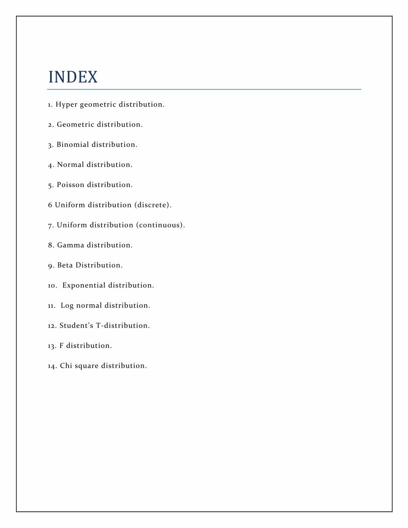
INDEX

1. Hyper geometric distribution.

2. Geometric distribution.

3. Binomial distribution.

4. Normal distribution.

5. Poisson distribution.

6 Uniform distribution (discrete).

7. Uniform distribution (continuous).

8. Gamma distribution.

9. Beta Distribution.

10. Exponential distribution.

11. Log normal distribution.

12. Student’s T-distribution.

13. F distribution.

14. Chi square distribution.

HYPER GEOMETRIC DISTRIBUTION

DEFINITION

A random variable X follows the hyper geometric distribution with

parameters N, m and n if its probability mass function is given by:

Where is the binomial coefficient; it is non-negative when

.

The hyper geometric distribution is a discrete probability distribution that describes the number

of successes in a sequence of ‘n’ draws from a finite population without replacement, just as

the binomial distribution describes the number of successes for draws with replacement.

APPLICATION

The classical application of the hyper geometric distribution is sampling without replacement.

Example: a pot with two types of marbles, black ones and white ones. Define drawing a white

marble as a success and drawing a black marble as a failure (analogous to the binomial

distribution). If the variable N describes the number of all marbles in the pot(see contingency

table below) and m describes the number of white marbles, then N − m corresponds to the

number of black marbles. In this example X is the random variable whose outcome is k, the

number of white marbles actually drawn in the experiment. This situation is illustrated by the

following contingency table:

drawn not drawn total

white marbles k m − k m

black marbles n − k N + k − n −

m N − m

Total n N − n N

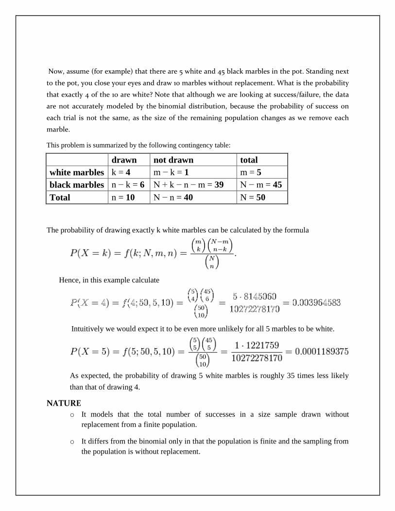
Now, assume (for example) that there are 5 white and 45 black marbles in the pot. Standing next

to the pot, you close your eyes and draw 10 marbles without replacement. What is the probability

that exactly 4 of the 10 are white? Note that although we are looking at success/failure, the data

are not accurately modeled by the binomial distribution, because the probability of success on

each trial is not the same, as the size of the remaining population changes as we remove each

marble.

This problem is summarized by the following contingency table:

drawn not drawn total

white marbles k = 4 m − k = 1 m = 5

black marbles n − k = 6 N + k − n − m = 39 N − m = 45

Total n = 10 N − n = 40 N = 50

The probability of drawing exactly k white marbles can be calculated by the formula

Hence, in this example calculate

Intuitively we would expect it to be even more unlikely for all 5 marbles to be white.

As expected, the probability of drawing 5 white marbles is roughly 35 times less likely

than that of drawing 4.

NATURE

o It models that the total number of successes in a size sample drawn without

replacement from a finite population.

o It differs from the binomial only in that the population is finite and the sampling from

the population is without replacement.

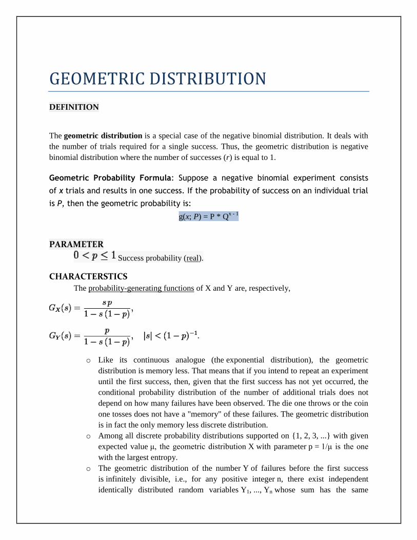
GEOMETRIC DISTRIBUTION

DEFINITION

The geometric distribution is a special case of the negative binomial distribution. It deals with

the number of trials required for a single success. Thus, the geometric distribution is negative

binomial distribution where the number of successes (r) is equal to 1.

Geometric Probability Formula: Suppose a negative binomial experiment consists

of x trials and results in one success. If the probability of success on an individual trial

is P, then the geometric probability is:

g(x; P) = P * Qx - 1

PARAMETER

Success probability (real).

CHARACTERSTICS

The probability-generating functions of X and Y are, respectively,

o Like its continuous analogue (the exponential distribution), the geometric

distribution is memory less. That means that if you intend to repeat an experiment

until the first success, then, given that the first success has not yet occurred, the

conditional probability distribution of the number of additional trials does not

depend on how many failures have been observed. The die one throws or the coin

one tosses does not have a "memory" of these failures. The geometric distribution

is in fact the only memory less discrete distribution.

o Among all discrete probability distributions supported on {1, 2, 3, ...} with given

expected value μ, the geometric distribution X with parameter p = 1/μ is the one

with the largest entropy.

o The geometric distribution of the number Y of failures before the first success

is infinitely divisible, i.e., for any positive integer n, there exist independent

identically distributed random variables Y1, ..., Yn whose sum has the same

distribution that Y has. These will not be geometrically distributed unless n = 1;

they follow a negative binomial distribution.

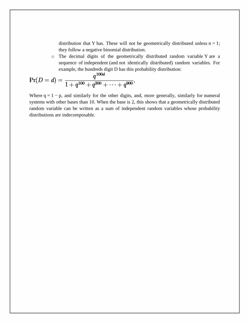
o The decimal digits of the geometrically distributed random variable Y are a

sequence of independent (and not identically distributed) random variables. For

example, the hundreds digit D has this probability distribution:

Where q = 1 − p, and similarly for the other digits, and, more generally, similarly for numeral

systems with other bases than 10. When the base is 2, this shows that a geometrically distributed

random variable can be written as a sum of independent random variables whose probability

distributions are indecomposable.

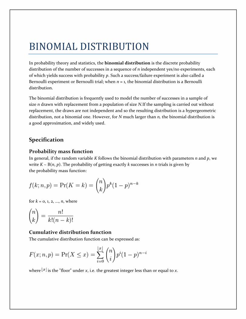
BINOMIAL DISTRIBUTION

In probability theory and statistics, the binomial distribution is the discrete probability

distribution of the number of successes in a sequence of n independent yes/no experiments, each

of which yields success with probability p. Such a success/failure experiment is also called a

Bernoulli experiment or Bernoulli trial; when n = 1, the binomial distribution is a Bernoulli

distribution.

The binomial distribution is frequently used to model the number of successes in a sample of

size n drawn with replacement from a population of size N.If the sampling is carried out without

replacement, the draws are not independent and so the resulting distribution is a hypergeometric

distribution, not a binomial one. However, for N much larger than n, the binomial distribution is

a good approximation, and widely used.

Specification

Probability mass function

In general, if the random variable K follows the binomial distribution with parameters n and p, we

write K ~ B(n, p). The probability of getting exactly k successes in n trials is given by

the probability mass function:

for k = 0, 1, 2, ..., n, where

Cumulative distribution function

The cumulative distribution function can be expressed as:

where is the "floor" under x, i.e. the greatest integer less than or equal to x.

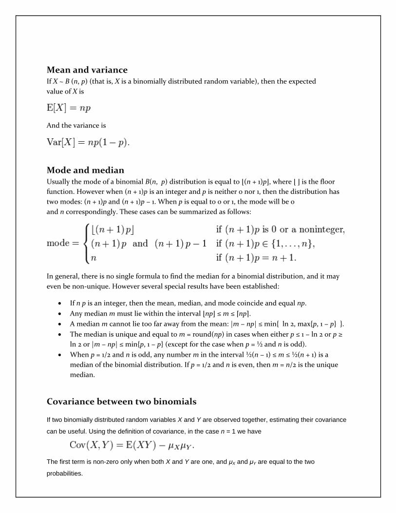
Mean and variance If X ~ B (n, p) (that is, X is a binomially distributed random variable), then the expected

value of X is

And the variance is

Mode and median Usually the mode of a binomial B(n,  p) distribution is equal to ⌊(n + 1)p⌋, where ⌊ ⌋ is the floor

function. However when (n + 1)p is an integer and p is neither 0 nor 1, then the distribution has

two modes: (n + 1)p and (n + 1)p − 1. When p is equal to 0 or 1, the mode will be 0

and n correspondingly. These cases can be summarized as follows:

In general, there is no single formula to find the median for a binomial distribution, and it may

even be non-unique. However several special results have been established:

If n p is an integer, then the mean, median, and mode coincide and equal np.

Any median m must lie within the interval ⌊np⌋ ≤ m ≤ ⌈np⌉.

A median m cannot lie too far away from the mean: |m − np| ≤ min{  ln 2, max{p, 1 − p}  }.

The median is unique and equal to m = round(np) in cases when either p ≤ 1 − ln 2 or p ≥

ln 2 or |m − np| ≤ min{p, 1 − p} (except for the case when p = ½ and n is odd).

When p = 1/2 and n is odd, any number m in the interval ½(n − 1) ≤ m ≤ ½(n + 1) is a

median of the binomial distribution. If p = 1/2 and n is even, then m = n/2 is the unique

median.

Covariance between two binomials

If two binomially distributed random variables X and Y are observed together, estimating their covariance

can be useful. Using the definition of covariance, in the case n = 1 we have

The first term is non-zero only when both X and Y are one, and μX and μY are equal to the two

probabilities.

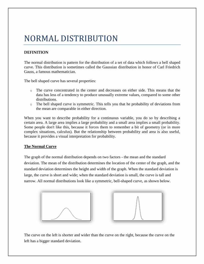
NORMAL DISTRIBUTION

DEFINITION

The normal distribution is pattern for the distribution of a set of data which follows a bell shaped

curve. This distribution is sometimes called the Gaussian distribution in honor of Carl Friedrich

Gauss, a famous mathematician.

The bell shaped curve has several properties:

o The curve concentrated in the center and decreases on either side. This means that the

data has less of a tendency to produce unusually extreme values, compared to some other

distributions.

o The bell shaped curve is symmetric. This tells you that he probability of deviations from

the mean are comparable in either direction.

When you want to describe probability for a continuous variable, you do so by describing a

certain area. A large area implies a large probability and a small area implies a small probability.

Some people don't like this, because it forces them to remember a bit of geometry (or in more

complex situations, calculus). But the relationship between probability and area is also useful,

because it provides a visual interpretation for probability.

The Normal Curve

The graph of the normal distribution depends on two factors - the mean and the standard

deviation. The mean of the distribution determines the location of the center of the graph, and the

standard deviation determines the height and width of the graph. When the standard deviation is

large, the curve is short and wide; when the standard deviation is small, the curve is tall and

narrow. All normal distributions look like a symmetric, bell-shaped curve, as shown below.

The curve on the left is shorter and wider than the curve on the right, because the curve on the

left has a bigger standard deviation.

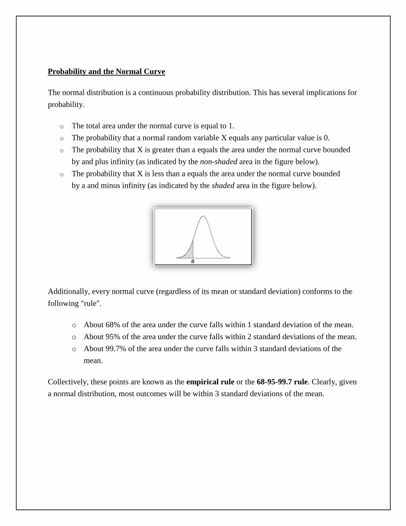
Probability and the Normal Curve

The normal distribution is a continuous probability distribution. This has several implications for

probability.

o The total area under the normal curve is equal to 1.

o The probability that a normal random variable X equals any particular value is 0.

o The probability that X is greater than a equals the area under the normal curve bounded

by and plus infinity (as indicated by the non-shaded area in the figure below).

o The probability that X is less than a equals the area under the normal curve bounded

by a and minus infinity (as indicated by the shaded area in the figure below).

Additionally, every normal curve (regardless of its mean or standard deviation) conforms to the

following "rule".

o About 68% of the area under the curve falls within 1 standard deviation of the mean.

o About 95% of the area under the curve falls within 2 standard deviations of the mean.

o About 99.7% of the area under the curve falls within 3 standard deviations of the

mean.

Collectively, these points are known as the empirical rule or the 68-95-99.7 rule. Clearly, given

a normal distribution, most outcomes will be within 3 standard deviations of the mean.

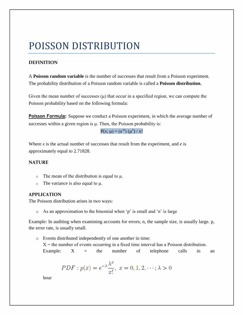
POISSON DISTRIBUTION

DEFINITION

A Poisson random variable is the number of successes that result from a Poisson experiment.

The probability distribution of a Poisson random variable is called a Poisson distribution.

Given the mean number of successes (μ) that occur in a specified region, we can compute the

Poisson probability based on the following formula:

Poisson Formula: Suppose we conduct a Poisson experiment, in which the average number of

successes within a given region is μ. Then, the Poisson probability is:

P(x; μ) = (e-μ

) (μx) / x!

Where x is the actual number of successes that result from the experiment, and e is

approximately equal to 2.71828.

NATURE

o The mean of the distribution is equal to μ.

o The variance is also equal to μ.

APPLICATION

The Poisson distribution arises in two ways:

o As an approximation to the binomial when ‘p’ is small and ‘n’ is large

Example: In auditing when examining accounts for errors; n, the sample size, is usually large. p,

the error rate, is usually small.

o Events distributed independently of one another in time:

X = the number of events occurring in a fixed time interval has a Poisson distribution.

Example: X = the number of telephone calls in an

hour

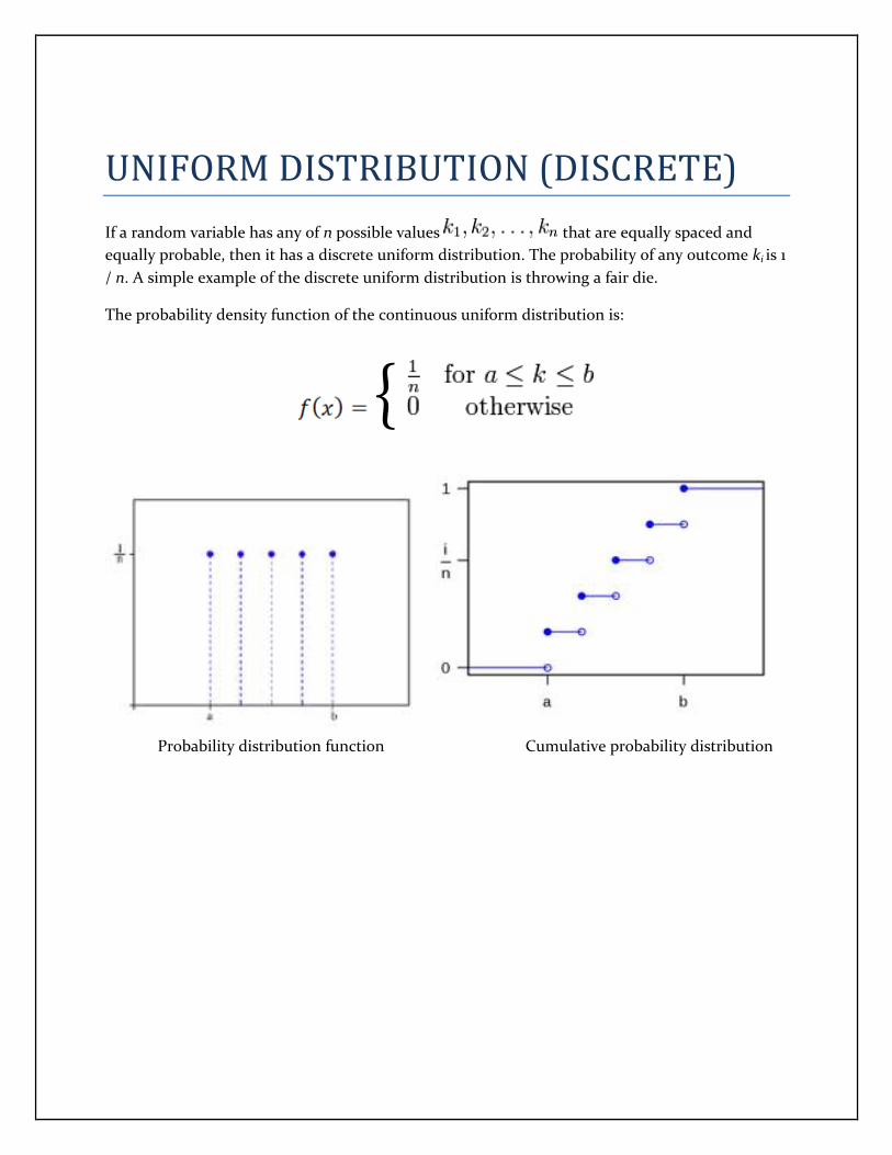
UNIFORM DISTRIBUTION (DISCRETE)

If a random variable has any of n possible values that are equally spaced and

equally probable, then it has a discrete uniform distribution. The probability of any outcome ki is 1

/ n. A simple example of the discrete uniform distribution is throwing a fair die.

The probability density function of the continuous uniform distribution is:

{

Probability distribution function Cumulative probability distribution

UNIFORM DISTRIBUTION (CONTINUOUS)

In probability theory and statistics, the continuous uniform distribution or rectangular

distribution is a family of probability distributions such that for each member of the family, all

intervals of the same length on the distribution's support are equally probable.

The probability density function of the continuous uniform distribution

is:

Probability distribution function Cumulative probability distribution

Application: One of the most important applications of the uniform distribution is in the generation of

random numbers. That is, almost all random number generators generate random numbers on

the (0, 1) interval.

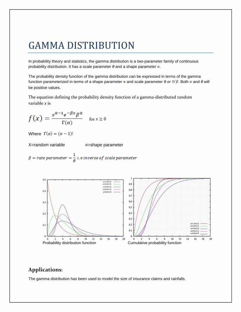
GAMMA DISTRIBUTION

In probability theory and statistics, the gamma distribution is a two-parameter family of continuous

probability distribution. It has a scale parameter θ and a shape parameter .

The probability density function of the gamma distribution can be expressed in terms of the gamma

function parameterized in terms of a shape parameter and scale parameter θ or 1/ . Both and θ will

be positive values.

The equation defining the probability density function of a gamma-distributed random

variable x is

for

Where

X=random variable =shape parameter

Probability distribution function Cumulative probability function

Applications:

The gamma distribution has been used to model the size of insurance claims and rainfalls.

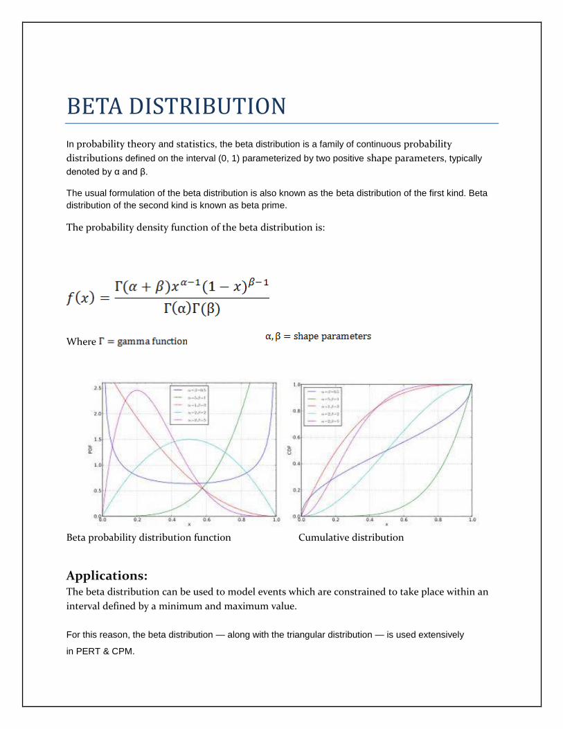
BETA DISTRIBUTION

In probability theory and statistics, the beta distribution is a family of continuous probability

distributions defined on the interval (0, 1) parameterized by two positive shape parameters, typically

denoted by α and β.

The usual formulation of the beta distribution is also known as the beta distribution of the first kind. Beta

distribution of the second kind is known as beta prime.

The probability density function of the beta distribution is:

Where

Beta probability distribution function Cumulative distribution

Applications: The beta distribution can be used to model events which are constrained to take place within an

interval defined by a minimum and maximum value.

For this reason, the beta distribution — along with the triangular distribution — is used extensively

in PERT & CPM.

EXPONENTIAL DISTRIBUTION

In probability theory and statistics, the exponential distribution (a.k.a. negative exponential

distribution) is a family of continuous probability distributions. It describes the time between

events in a Poisson process, i.e. a process in which events occur continuously and independently

at a constant average rate.

Characterization

Probability density function

The probability density function (pdf) of an exponential distribution

is

Alternatively, this can be defined using the Heaviside step function, H(x).

Here λ > 0 is the parameter of the distribution, often called the rate parameter. The distribution is

supported on the interval [0, ∞). If a random variable Xhas this distribution, we write X ~

Exp(λ).The exponential distribution exhibits infinite divisibility.

Cumulative distribution function

The cumulative distribution function is given by

Alternatively, this can be defined using the Heaviside step function,

H(x).

Properties

Mean, variance, and median

The mean or expected value of an exponentially distributed random variable X with rate

parameter λ is given by

In light of the examples given above, this makes sense: if you receive phone calls at an average

rate of 2 per hour, then you can expect to wait half an hour for every call.

The variance of X is given by

The median of X is given by

Where, ln refers to the natural logarithm. Thus the absolute difference between the mean and

median is

In accordance with the median-mean inequality.

Applications

Occurrence of EVENTS The exponential distribution occurs naturally when describing the lengths of the inter-

arrival times in a homogeneous Poisson process.

Exponential variables can also be used to model situations where certain events occur

with a constant probability per unit length, such as the distance between mutations on a

DNA strand, or between roadkills on a given road.

In queuing theory, the service times of agents in a system (e.g. how long it takes for a bank

teller etc. to serve a customer) are often modeled as exponentially distributed variables.

In physics, if you observe a gas at a fixed temperature and pressure in a uniform

gravitational field, the heights of the various molecules also follow an approximate

exponential distribution. This is a consequence of the entropy property mentioned below.

In hydrology, the exponential distribution is used to analyze extreme values of such

variables as monthly and annual maximum values of daily rainfall and river discharge

volumes.

LOG NORMAL DISTRIBUTION

In probability theory, a log-normal distribution is a probability distribution of a random variable

whose logarithm is normally distributed. If X is a random variable with a normal distribution,

then Y = exp(X) has a log-normal distribution; likewise, if Y is log-normally distributed, then X =

log(Y) is normally distributed. (This is true regardless of the base of the logarithmic function: if

loga(Y) is normally distributed, then so is logb(Y), for any two positive numbers a, b ≠ 1.

A variable might be modeled as log-normal if it can be thought of as the multiplicative product of

many independent random variables each of which is positive. For example, in finance, the

variable could represent the compound return from a sequence of many trades (each expressed as

its return + 1); or a long-term discount factor can be derived from the product of short-term

discount factors. In wireless communication, the attenuation caused by shadowing or slow fading

from random objects is often assumed to be log-normally distributed: see log-distance path loss

model.

μ and σ In a log-normal distribution, the parameters denoted μ and σ, are the mean and standard

deviation, respectively, of the variable’s natural logarithm (by definition, the variable’s logarithm

is normally distributed). On a non-logarithmized scale, μ and σ can be called the location

parameter and the scale parameter, respectively.

Characterization

Probability density function

The probability density function of a log-normal distribution

is:

This follows by applying the change-of-variables rule on the density function of a normal

distribution.

Cumulative distribution function

where erfc is the complementary error function, and Φ is the standard normal cdf.

Properties

Location and scale

For the log-normal distribution, the location and scale properties of the distribution are more

readily treated using the geometric mean and geometric standard deviation than the arithmetic

mean and standard deviation.

Geometric moments The geometric mean of the log-normal distribution is eμ. Because the log of a log-normal variable

is symmetric and quantiles are preserved under monotonic transformations, the geometric mean

of a log-normal distribution is equal to its median.The geometric mean (mg) can alternatively be

derived from the arithmetic mean (ma) in a log-normal distribution by:

The geometric standard deviation is equal to eσ.

Arithmetic moments

If X is a lognormally distributed variable, its expected value (E - which can be assumed to

represent the arithmetic mean), variance (Var), and standard deviation (s.d.) are

Equivalently, parameters μ and σ can be obtained if the expected value and variance are known:

For any real or complex number s, the sth moment of log-normal X is given by

A log-normal distribution is not uniquely determined by its moments E[Xk] for k ≥ 1, that is, there

exists some other distribution with the same moments for all k. In fact, there is a whole family of

distributions with the same moments as the log-normal distribution.

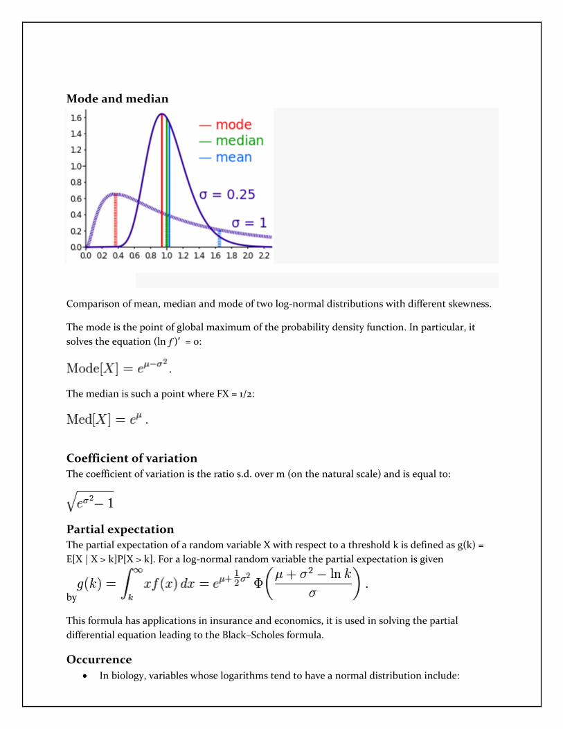
Mode and median

Comparison of mean, median and mode of two log-normal distributions with different skewness.

The mode is the point of global maximum of the probability density function. In particular, it

solves the equation (ln ƒ)′ = 0:

The median is such a point where FX = 1/2:

Coefficient of variation

The coefficient of variation is the ratio s.d. over m (on the natural scale) and is equal to:

Partial expectation

The partial expectation of a random variable X with respect to a threshold k is defined as g(k) =

E[X | X > k]P[X > k]. For a log-normal random variable the partial expectation is given

by

This formula has applications in insurance and economics, it is used in solving the partial

differential equation leading to the Black–Scholes formula.

Occurrence

In biology, variables whose logarithms tend to have a normal distribution include:

o Measures of size of living tissue (length, height, skin area, weight);The length of

inert appendages (hair, claws, nails, teeth) of biological specimens, in the direction

of growth;[citation needed]

o Certain physiological measurements, such as blood pressure of adult humans

(after separation on male/female subpopulations).

o Subsequently, reference ranges for measurements in healthy individuals are more

accurately estimated by assuming a log-normal distribution than by assuming a

symmetric distribution about the mean.

In hydrology, the log-normal distribution is used to analyze extreme values of such

variables as monthly and annual maximum values of daily rainfall and river discharge

volumes.

In finance, in particular the Black–Scholes model, changes in the logarithm of exchange

rates, price indices, and stock market indices are assumed normal (these variables behave

like compound interest, not like simple interest, and so are multiplicative).

In Reliability analysis, the lognormal distribution is often used to model times to repair a

maintainable system.

It has been proposed that coefficients of friction and wear may be treated as having a lognormal

distribution.

STUDENT’S T- DISTRIBUTION

DEFINITION

According to the central limit theorem, the sampling distribution of a statistic (like a sample

mean) will follow a normal distribution, as long as the sample size is sufficiently large.

Therefore, when we know the standard deviation of the population, we can compute a z-score,

and use the normal distribution to evaluate probabilities with the sample mean.

But sample sizes are sometimes small, and often we do not know the standard deviation of the

population. When either of these problems occur, statisticians rely on the distribution of the t

statistic(also known as the t score), whose values are given by:

t = [ x - μ ] / [ s / sqrt( n ) ]

where x is the sample mean, μ is the population mean, s is the standard deviation of the sample,

and n is the sample size. The distribution of the t statistic is called the t distribution or

the Student t distribution.

Degrees of Freedom

There are actually many different t distributions. The particular form of the t distribution is

determined by its degrees of freedom. The degree of freedom refers to the number of

independent observations in a set of data.

When estimating a mean score or a proportion from a single sample, the number of independent

observations is equal to the sample size minus one. Hence, the distribution of the t statistic from

samples of size 8 would be described by a t distribution having 8 - 1 or 7 degrees of freedom.

Similarly, a t distribution having 15 degrees of freedom would be used with a sample of size 16.

NATURE

The t distribution has the following properties:

o The mean of the distribution is equal to 0 .

o The variance is equal to v / ( v - 2 ), where v is the degrees of freedom (see last

section) and v> 2.

o The variance is always greater than 1, although it is close to 1 when there are

many degrees of freedom. With infinite degrees of freedom, the t distribution is

the same as the standard normal distribution.

APPLICATION

The t distribution can be used with any statistic having a bell-shaped distribution (i.e.,

approximately normal). The central limit theorem states that the sampling distribution of a

statistic will be normal or nearly normal, if any of the following conditions apply.

o The population distribution is normal.

o The sampling distribution is symmetric, unimodal, without outliers, and the sample

size is 15 or less.

o The sampling distribution is moderately skewed, unimodal, without outliers, and the

sample size is between 16 and 40.

o The sample size is greater than 40, without outliers.

The t distribution should not be used with small samples from populations that are not

approximately normal.

EXAMPLE: Suppose scores on an IQ test are normally distributed, with a mean of 100.

Suppose 20 people are randomly selected and tested. The standard deviation in the sample group

is 15. What is the probability that the average test score in the sample group will be at most 110?

Solution:

To solve this problem, we will work directly with the raw data from the problem. We will not

compute the t score; the T Distribution Calculator will do that work for us. Since we will work

with the raw data, we select "Sample mean" from the Random Variable dropdown box. Then, we

enter the following data:

o The degrees of freedom are equal to 20 - 1 = 19.

o The population mean equals 100.

o The sample mean equals 110.

o The standard deviation of the sample is 15.

We enter these values into the T Distribution Calculator. The calculator displays the cumulative

probability: 0.996. Hence, there is a 99.6% chance that the sample average will be no greater

than 110.

F-DISTRIBUTION

DEFINITION

The distribution of all possible values of the f statistic is called an F distribution, with v1 = n1 - 1

andv2 = n2 - 1 degrees of freedom.

The curve of the F distribution depends on the degrees of freedom, v1 and v2. When describing an

F distribution, the number of degrees of freedom associated with the standard deviation in the

numerator of the f statistic is always stated first. Thus, f(5, 9) would refer to an F distribution

with v1= 5 and v2 = 9 degrees of freedom; whereas f(9, 5) would refer to an F distribution

with v1 = 9 and v2 = 5 degrees of freedom. Note that the curve represented by f(5, 9) would differ

from the curve represented by f(9, 5).

PARAMETER

degree of freedom

NATURE

The F distribution has the following nature:

The mean of the distribution is equal to v2 / ( v2 - 2 ) for v2 > 2.

The variance is equal to [ 2 * v22 * ( v1 + v1 - 2 ) ] / [ v1 * ( v2 - 2 )

2 * ( v2 - 4 ) ] for v2 > 4.

EXAMPLE: Find the cumulative probability associated with each of the f statistics from

Example 1, above.

Solution: To solve this problem, we need to find the degrees of freedom for each sample. Then,

we will use the F Distribution Calculator to find the probabilities.

The degrees of freedom for the sample of women are equal to n - 1 = 7 - 1 = 6.

The degrees of freedom for the sample of men are equal to n - 1 = 12 - 1 = 11.

Therefore, when the women's data appear in the numerator, the numerator degrees of

freedom v1 is equal to 6; and the denominator degrees of freedom v2 is equal to 11. And, based

on the computations shown in the previous example, the f statistic is equal to 1.68. We plug these

values into the F Distribution Calculator and find that the cumulative probability is 0.78.

On the other hand, when the men's data appear in the numerator, the numerator degrees of

freedom v1 is equal to 11; and the denominator degrees of freedom v2 is equal to 6. And, based

on the computations shown in the previous example, the f statistic is equal to 0.595. We plug

these values into the F Distribution Calculator and find that the cumulative probability is 0.22.

CHI SQUARE DISTRIBUTION

Definition If Z1, ..., Zk are independent, standard normal random variables, then the sum of their squares,

is distributed according to the chi-squared distribution with k degrees of freedom. This is usually

denoted as

The chi-squared distribution has one parameter: k — a positive integer that specifies the number

of degrees of freedom (i.e. the number of Zi’s)

The chi-squared distribution is a special case of the gamma distribution.

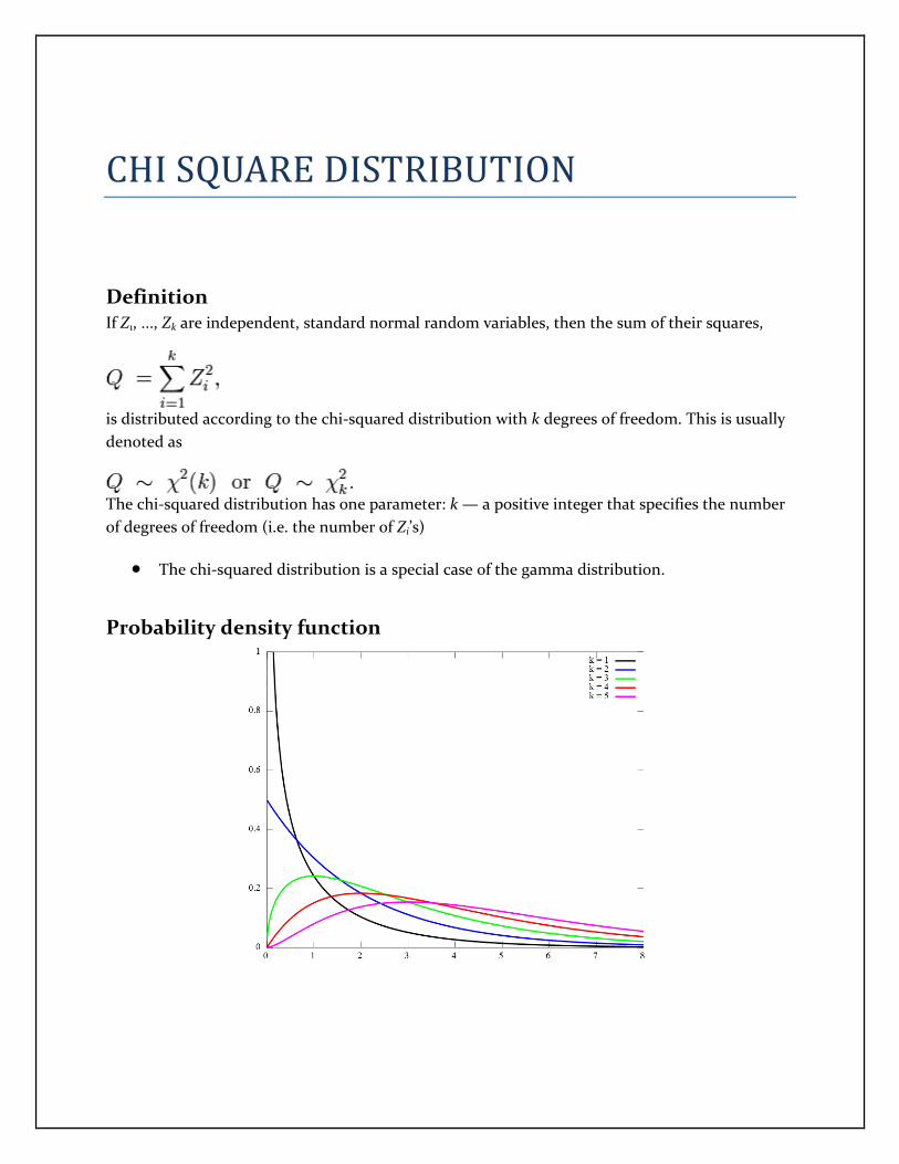
Probability density function

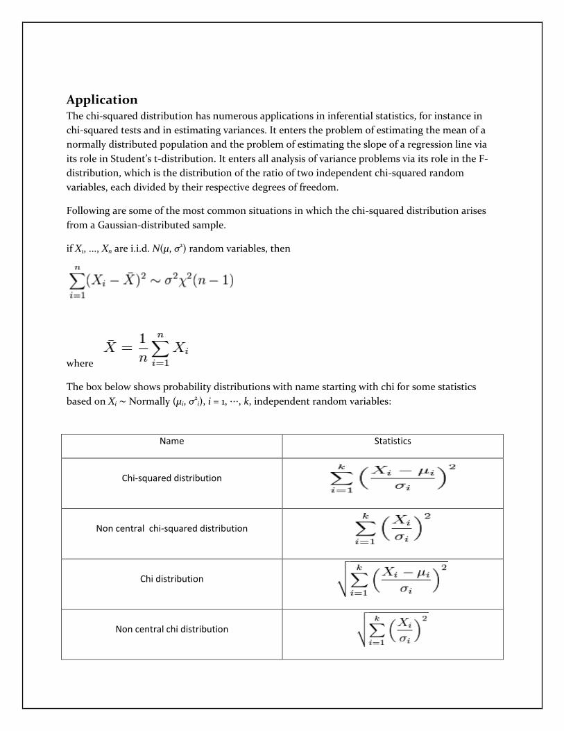
Application The chi-squared distribution has numerous applications in inferential statistics, for instance in

chi-squared tests and in estimating variances. It enters the problem of estimating the mean of a

normally distributed population and the problem of estimating the slope of a regression line via

its role in Student’s t-distribution. It enters all analysis of variance problems via its role in the F-

distribution, which is the distribution of the ratio of two independent chi-squared random

variables, each divided by their respective degrees of freedom.

Following are some of the most common situations in which the chi-squared distribution arises

from a Gaussian-distributed sample.

if X1, ..., Xn are i.i.d. N(μ, σ2) random variables, then

where

The box below shows probability distributions with name starting with chi for some statistics

based on Xi ∼ Normally (μi, σ2

i), i = 1, ⋯, k, independent random variables:

Name Statistics

Chi-squared distribution

Non central chi-squared distribution

Chi distribution

Non central chi distribution

Table of Χ2 Value Vs. P-Value The p-value is the probability of observing a test statistic at least as extreme in a chi-squared

distribution. Accordingly, since the cumulative distribution function (CDF) for the appropriate

degrees of freedom (df) gives the probability of having obtained a value less extreme than this

point, subtracting the CDF value from 1 gives the p-value. The table below gives a number of p-

values matching to χ2 for the first 10 degrees of freedom.

A p-value of 0.05 or less is usually regarded as statistically significant, i.e. the observed deviation

from the null hypothesis is significant.

REFERENCE

1. http://www.wolframalpha.com/input/?i=inverse+p+%3D+1+-+e^-l

2. http://stattrek.com/Lesson2/Normal.aspx?Tutorial=Stat

3. http://en.wikipedia.org/wiki/Poisson_distribution