QBM117Business Statistics

Probability and Probability Distributions

Continuous Probability Distributions

1

Objectives• To differentiate between a discrete probability

distribution and a continuous probability distribution

• To introduce the probability density function and its relationship to a continuous random variable

• To introduce the uniform distribution

• To introduce the normal distribution

• To introduce the standard normal random variable

• Use the standard normal tables to find probabilities2

Continuous Random Variables

• A continuous random variable has an infinite number of possible values.

• It can assume any value in an interval.

• We cannot list all the possible values of a continuous random variable.

3

Continuous Probability Distribution

• A continuous random variable has an infinite number of possible values.

• It is not possible to calculate the probability that a continuous random variable will take on a specific value.

• Instead we calculate the probability that a continuous random variable will lie in a specific interval.

4

Probability Density Function

• A smooth curve is used to represent the probability distribution of a continuous random variable.

• The curve is called a probability density function and is denoted by .)(xf

5

• A probability density function must satisfy two conditions:

1. is non-negative,

2. The total area under the curve is equal to 1

( )f x

( )f x

( )f x

( ) 0f x

6

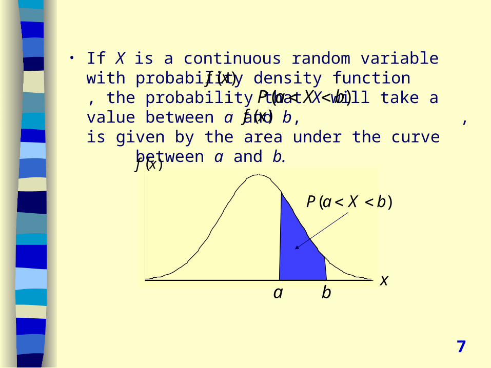
• If X is a continuous random variable with probability density function , the probability that X will take a value between a and b, , is given by the area under the curve between a and b.

( )f x( )P a X b

( )f x

( )f x

xa b

( )P a X b

7

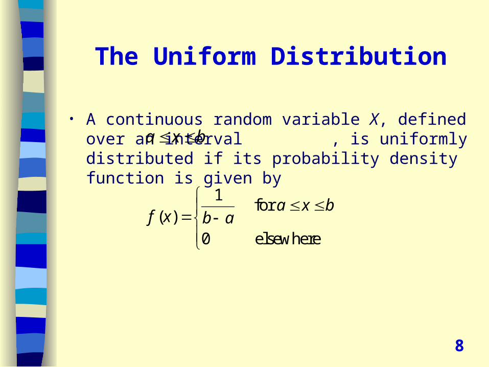
The Uniform Distribution

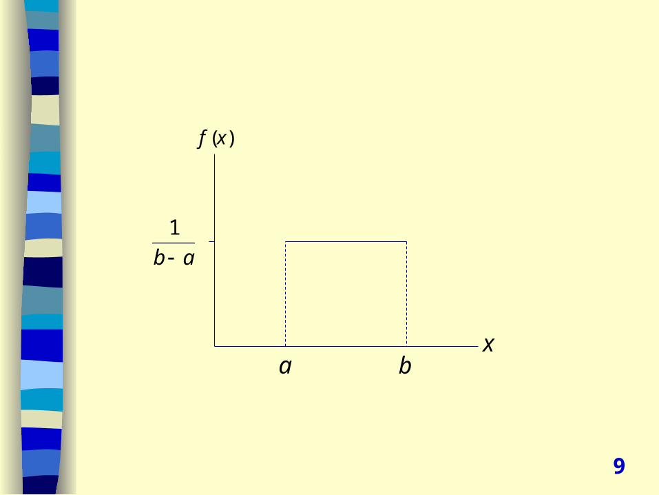
• A continuous random variable X, defined over an interval , is uniformly distributed if its probability density function is given by

1 for

( )0 elsewhere

a x bf x b a

a x b

8

a b

1

b a

( )f x

x

9

10

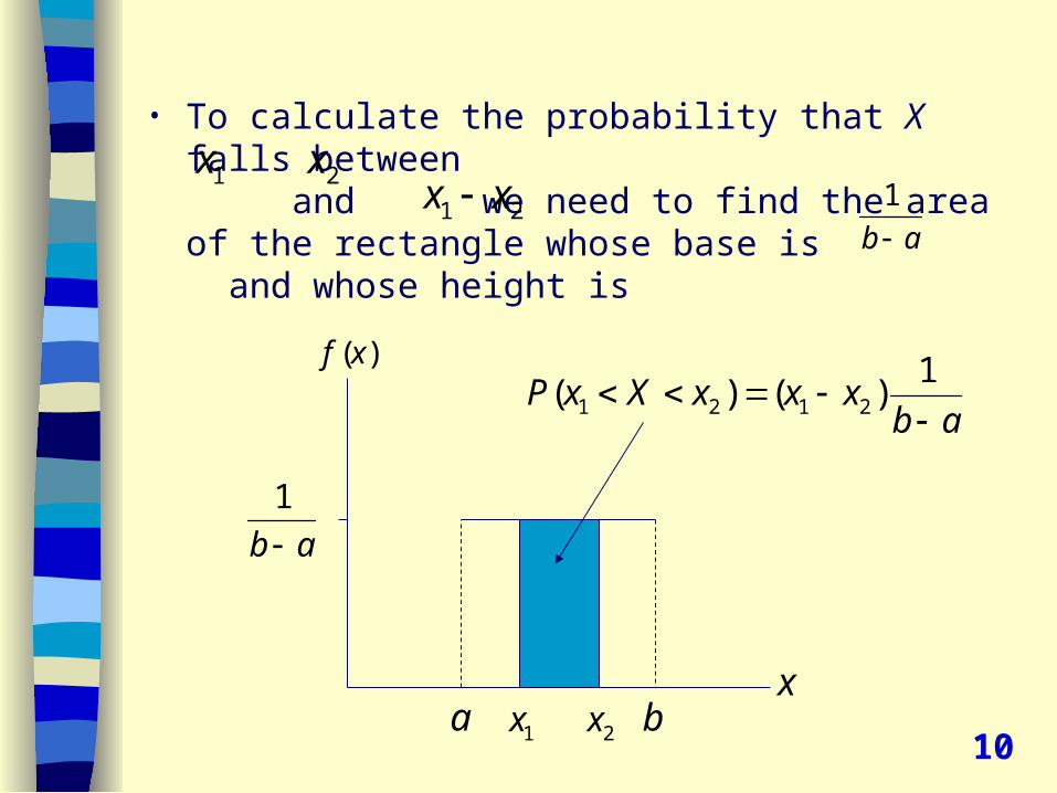
• To calculate the probability that X falls between and we need to find the area of the rectangle whose base is and whose height is

1x 2x

( )f x

xa b

1

b a

1x 2x

1 2x x 1

b a

1 2 1 2

1( ) ( )P x X x x x

b a

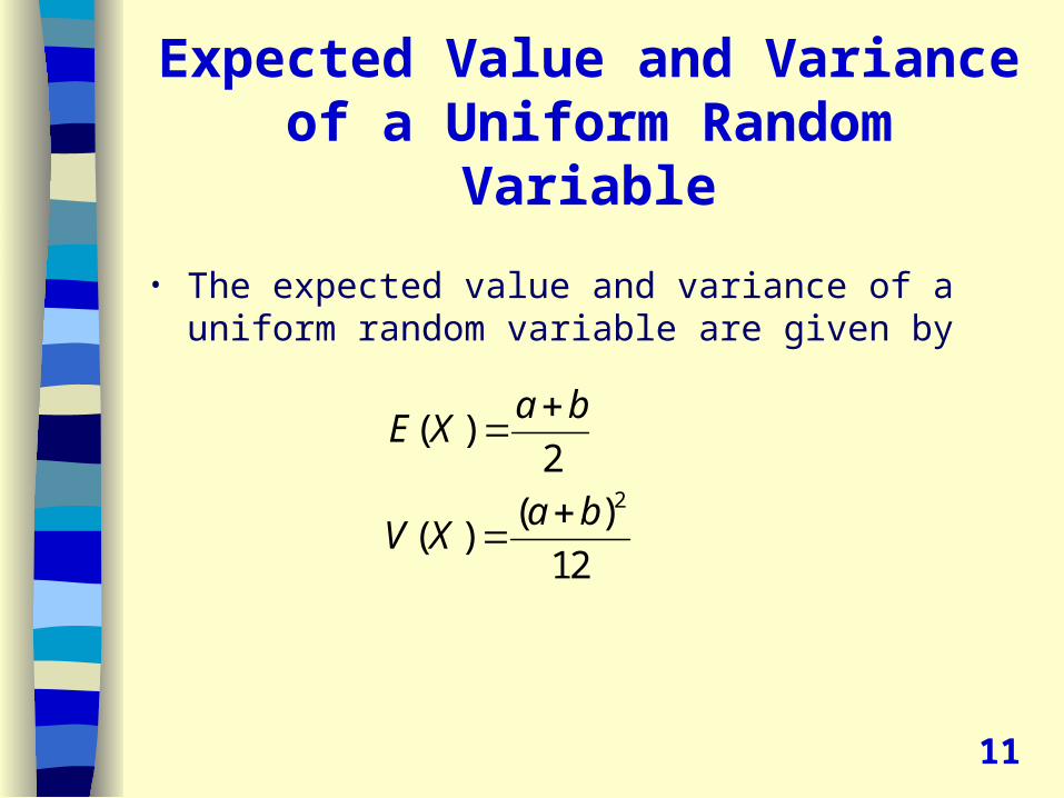
Expected Value and Variance of a Uniform Random Variable

• The expected value and variance of a uniform random variable are given by

11

2

( )2

( )( )

12

a bE X

a bV X

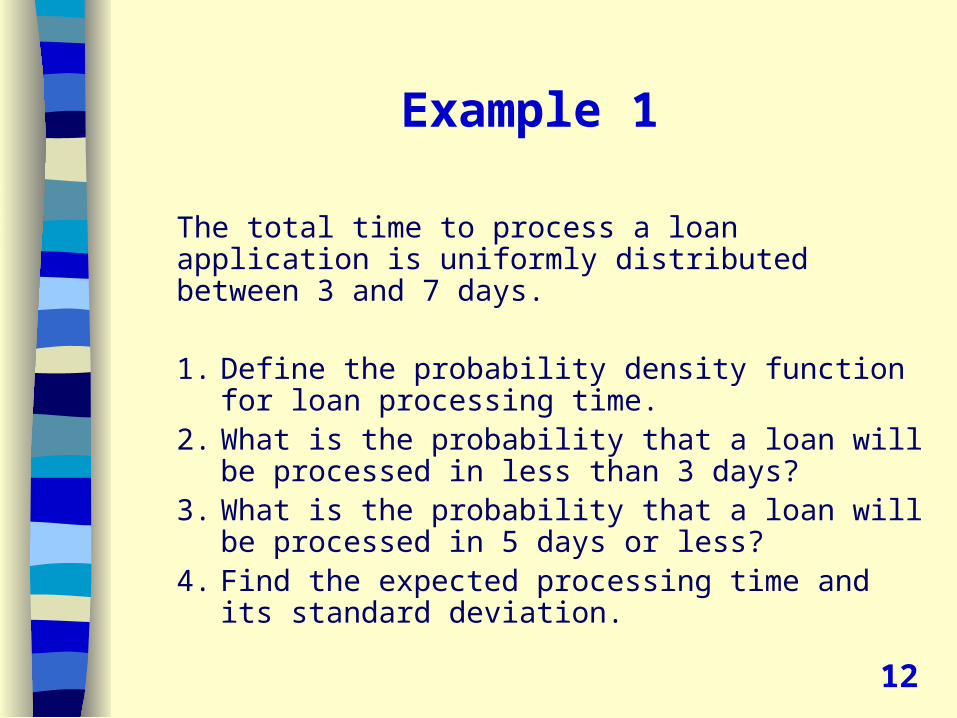
Example 1

The total time to process a loan application is uniformly distributed between 3 and 7 days.

1. Define the probability density function for loan processing time.

2. What is the probability that a loan will be processed in less than 3 days?

3. What is the probability that a loan will be processed in 5 days or less?

4. Find the expected processing time and its standard deviation.

12

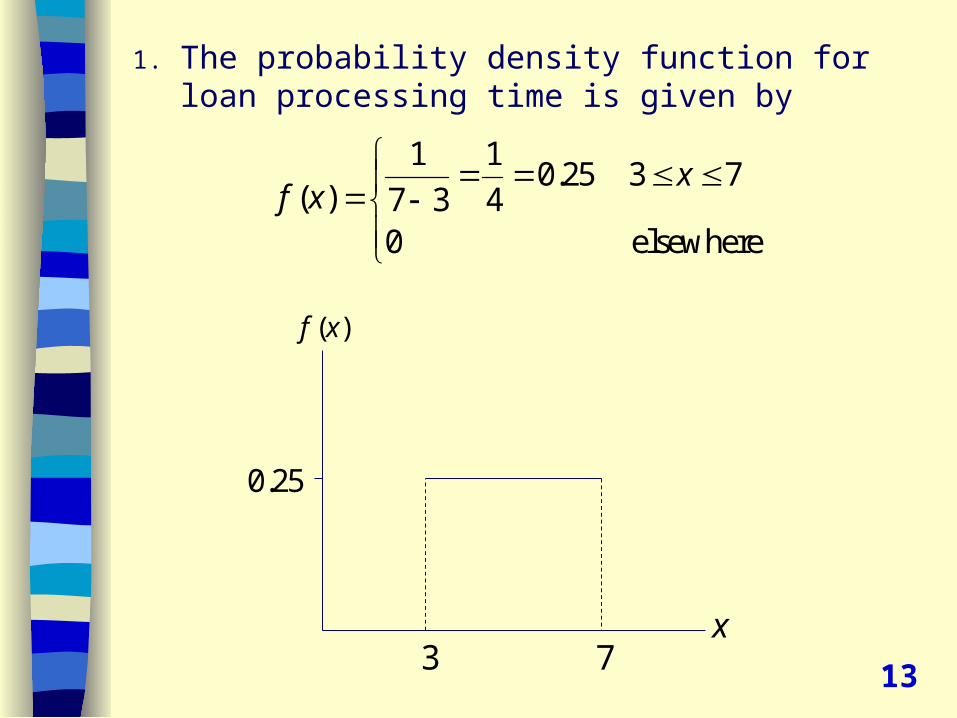
1. The probability density function for loan processing time is given by

1 10.25 3 7

( ) 7 3 40 elsewhere

xf x

( )f x

x3 7

0.25

13

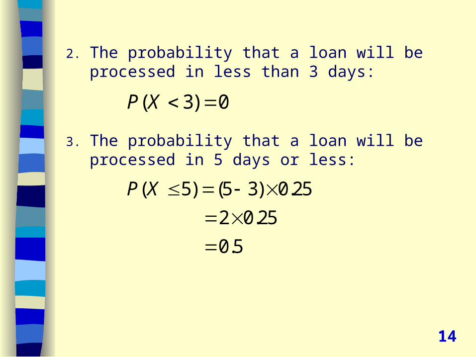
2. The probability that a loan will be processed in less than 3 days:

3. The probability that a loan will be processed in 5 days or less:

( 3) 0P X

( 5) (5 3) 0.25

2 0.25

0.5

P X

14

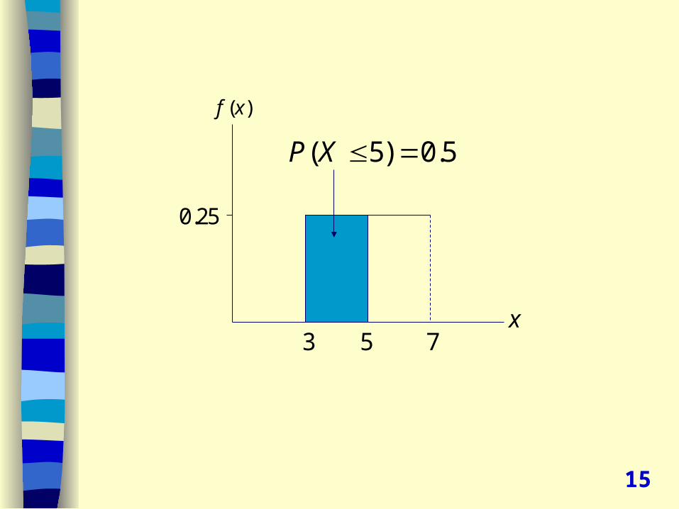
( )f x

x3 7

0.25

5

( 5) 0.5P X

15

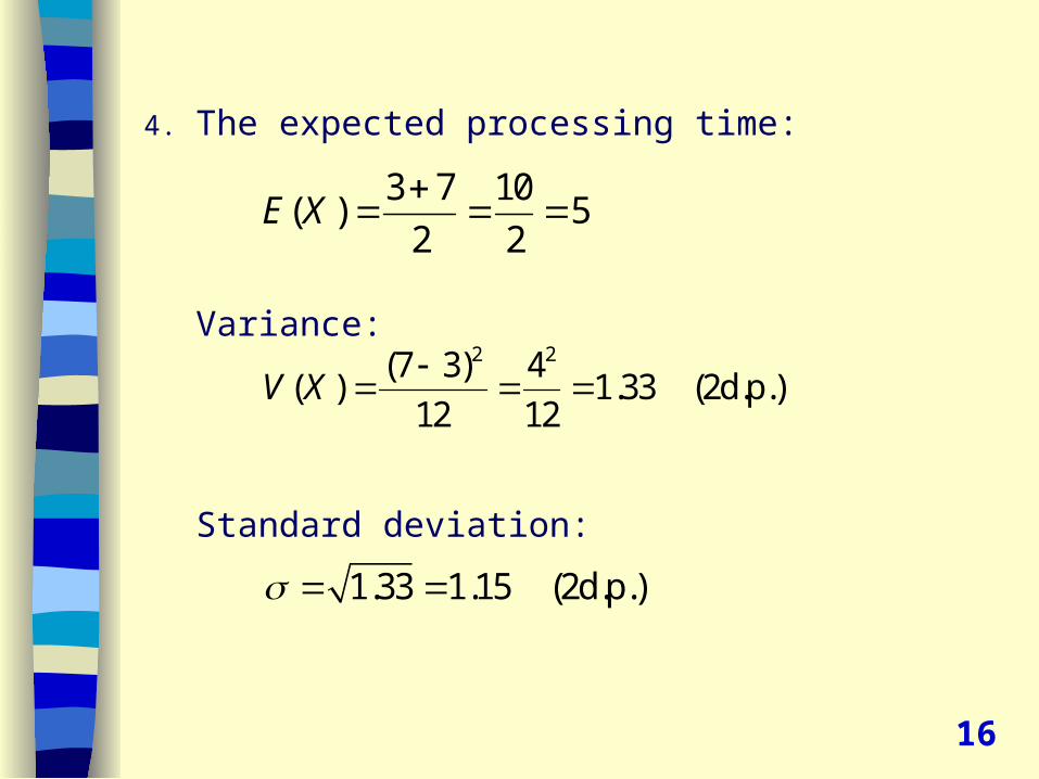
4. The expected processing time:

Variance:

Standard deviation:

3 7 10( ) 5

2 2E X

2 2(7 3) 4( ) 1.33 (2d.p.)

12 12V X

1.33 1.15 (2d.p.)

16

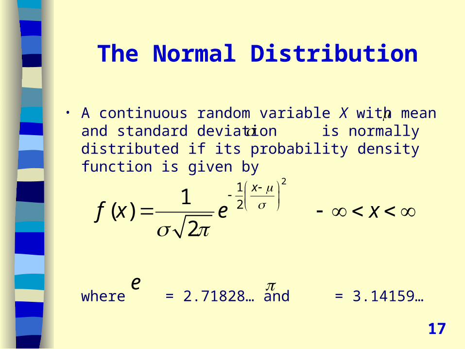
The Normal Distribution

• A continuous random variable X with mean and standard deviation is normally distributed if its probability density function is given by

where = 2.71828… and = 3.14159…

17

21

21( )

2

x

f x e x

e

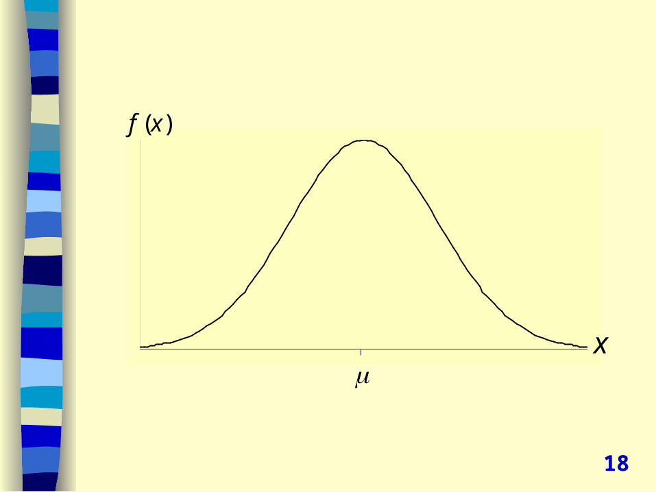
( )f x

x

18

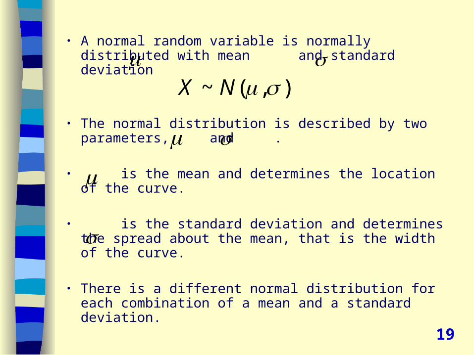
• A normal random variable is normally distributed with mean and standard deviation

• The normal distribution is described by two parameters, and .

• is the mean and determines the location of the curve.

• is the standard deviation and determines the spread about the mean, that is the width of the curve.

• There is a different normal distribution for each combination of a mean and a standard deviation.

19

~ ( , )X N

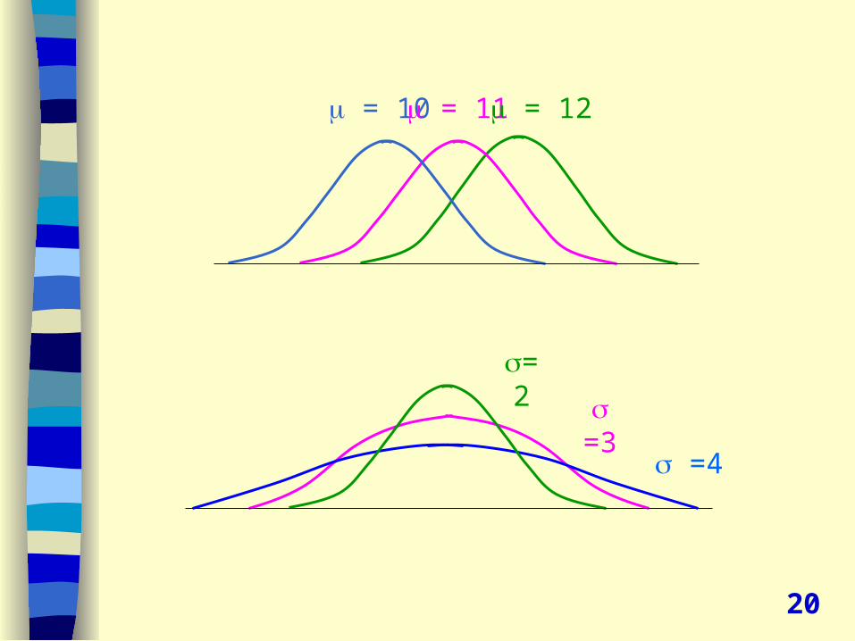
= 10 = 11 = 12

= 2

=3 =4

20

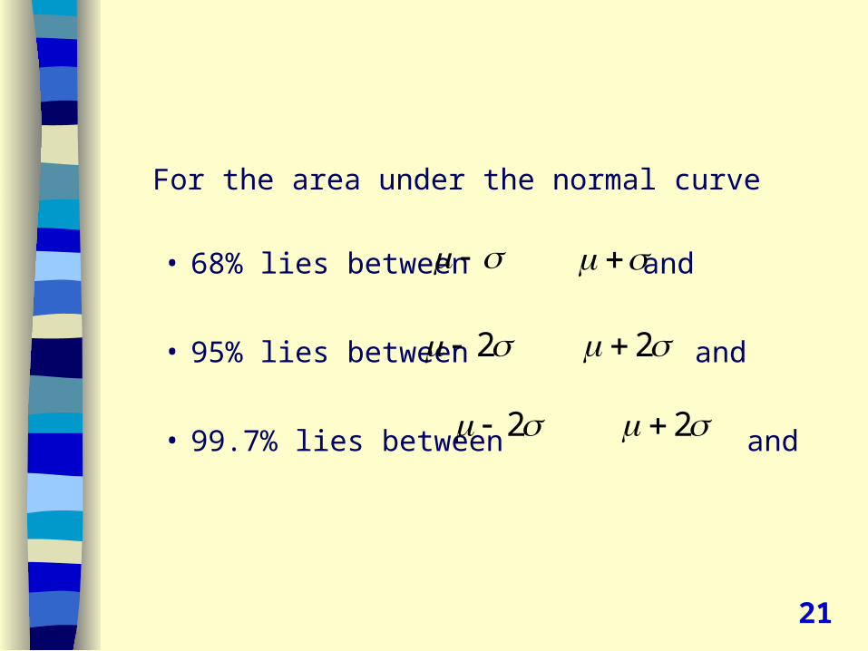
For the area under the normal curve

• 68% lies between and

• 95% lies between and

• 99.7% lies between and

2 2

2 2

21

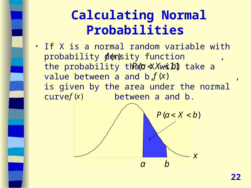
Calculating Normal Probabilities

• If X is a normal random variable with probability density function , the probability that X will take a value between a and b, , is given by the area under the normal curve between a and b.

( )f x( )P a X b

( )f x

( )f x

xa b

( )P a X b

22

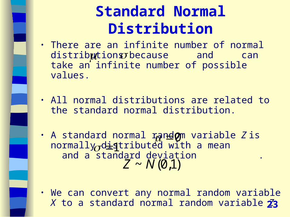
Standard Normal Distribution

• There are an infinite number of normal distributions because and can take an infinite number of possible values.

• All normal distributions are related to the standard normal distribution.

• A standard normal random variable Z is normally distributed with a mean and a standard deviation .

• We can convert any normal random variable X to a standard normal random variable Z.

23

0 1

~ (0,1)Z N

Standard Normal Probability Table

• Areas under the standard normal probability density function have been calculated and are available in Table 3 of Appendix 3 of the text.

• This table gives the probability that the standard normal random variable Z lies between 0 and z.

24

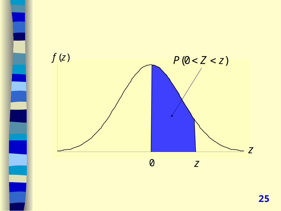
0 z

(0 )P Z z ( )f zz

25

Using Table 3

• Always draw a diagram.

• Shade in the area representing the probability you are trying to find.

26

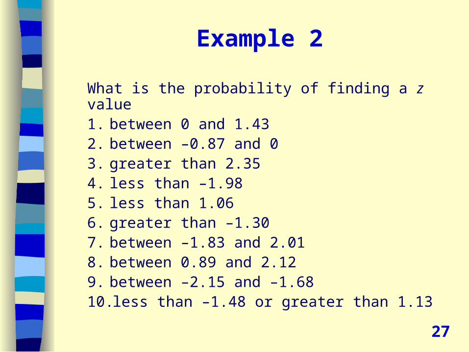
Example 2

What is the probability of finding a z value1. between 0 and 1.432. between –0.87 and 03. greater than 2.354. less than –1.985. less than 1.066. greater than –1.307. between –1.83 and 2.018. between 0.89 and 2.129. between –2.15 and –1.6810. less than –1.48 or greater than 1.13

27

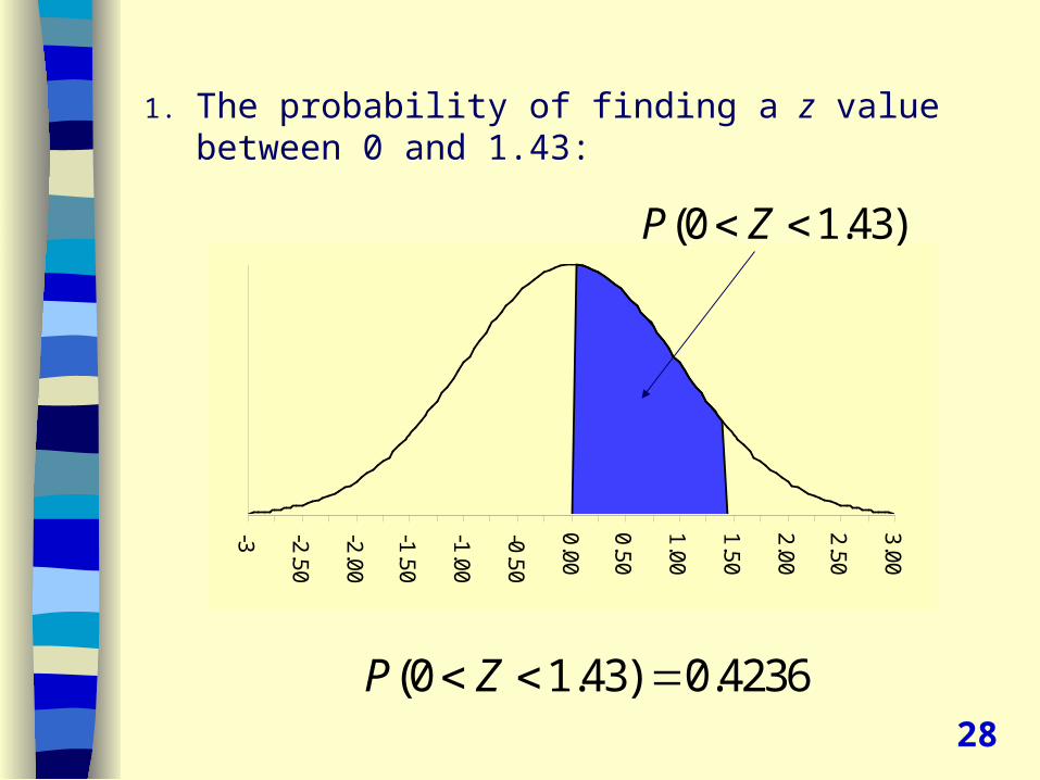
1. The probability of finding a z value between 0 and 1.43:

-3 -2.50

-2.00

-1.50

-1.00

-0.50

0.00

0.50

1.00

1.50

2.00

2.50

3.00

(0 1.43)P Z

(0 1.43) 0.4236P Z 28

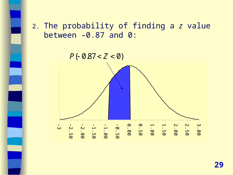
2. The probability of finding a z value between –0.87 and 0:

-3 -2.50

-2.00

-1.50

-1.00

-0.50

0.00

0.50

1.00

1.50

2.00

2.50

3.00

( 0.87 0)P Z

29

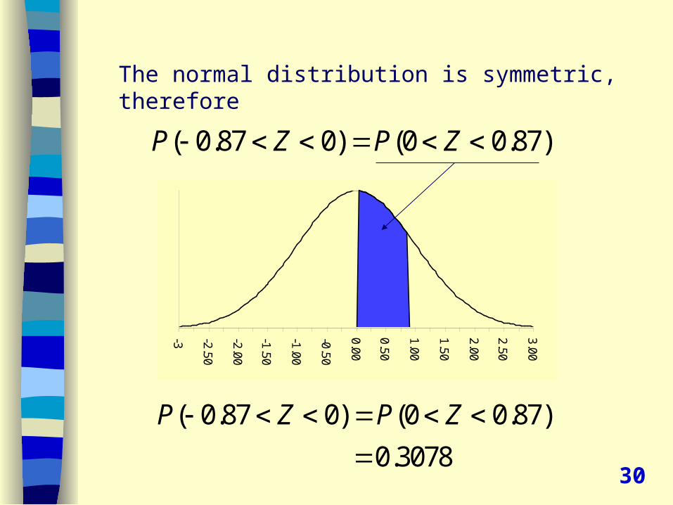
The normal distribution is symmetric, therefore

( 0.87 0) (0 0.87)P Z P Z

-3 -2.50

-2.00

-1.50

-1.00

-0.50

0.00

0.50

1.00

1.50

2.00

2.50

3.00

( 0.87 0) (0 0.87)

0.3078

P Z P Z

30

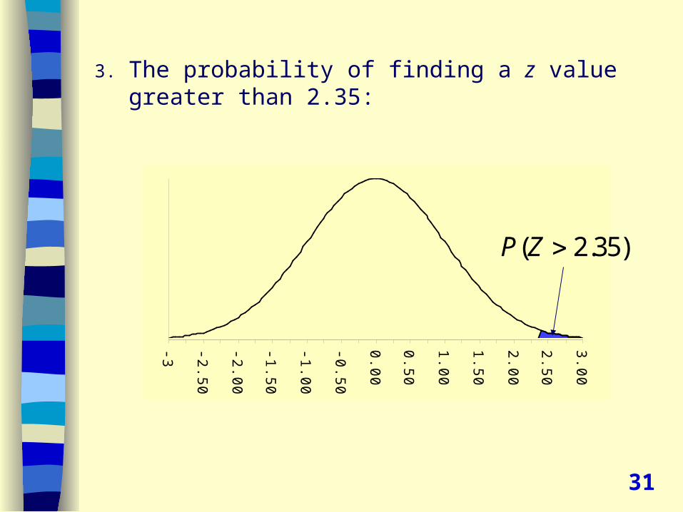
3. The probability of finding a z value greater than 2.35:

-3 -2.50

-2.00

-1.50

-1.00

-0.50

0.00

0.50

1.00

1.50

2.00

2.50

3.00

( 2.35)P Z

31

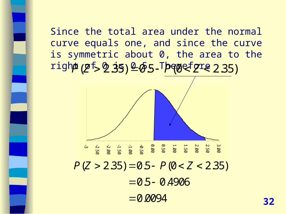
Since the total area under the normal curve equals one, and since the curve is symmetric about 0, the area to the right of 0 is 0.5. Therefore

( 2.35) 0.5 (0 2.35)P Z P Z

-3 -2.50

-2.00

-1.50

-1.00

-0.50

0.00

0.50

1.00

1.50

2.00

2.50

3.00

( 2.35) 0.5 (0 2.35)

0.5 0.4906

0.0094

P Z P Z 32

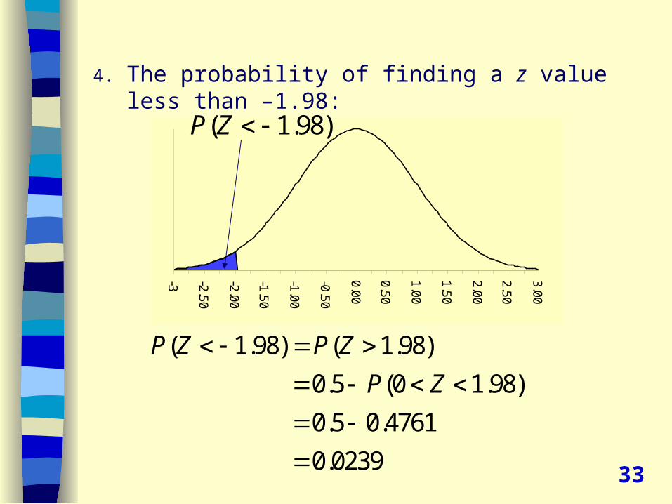
4. The probability of finding a z value less than –1.98:

-3 -2.50

-2.00

-1.50

-1.00

-0.50

0.00

0.50

1.00

1.50

2.00

2.50

3.00( 1.98)P Z

( 1.98) ( 1.98)

0.5 (0 1.98)

0.5 0.4761

0.0239

P Z P Z

P Z

33

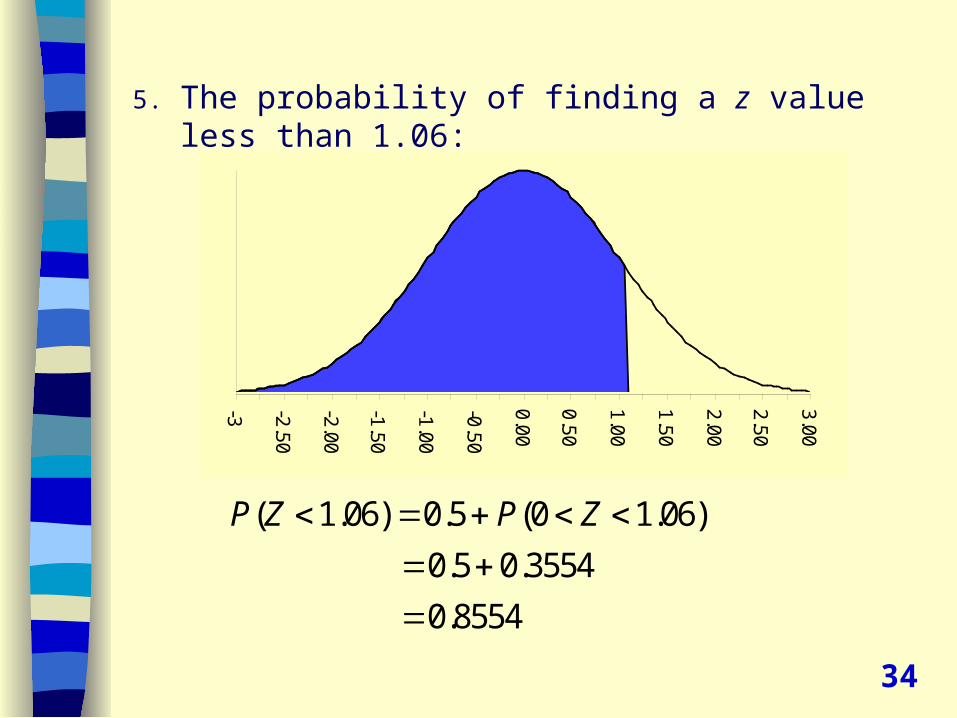
5. The probability of finding a z value less than 1.06:

-3 -2.50

-2.00

-1.50

-1.00

-0.50

0.00

0.50

1.00

1.50

2.00

2.50

3.00

( 1.06) 0.5 (0 1.06)

0.5 0.3554

0.8554

P Z P Z

34

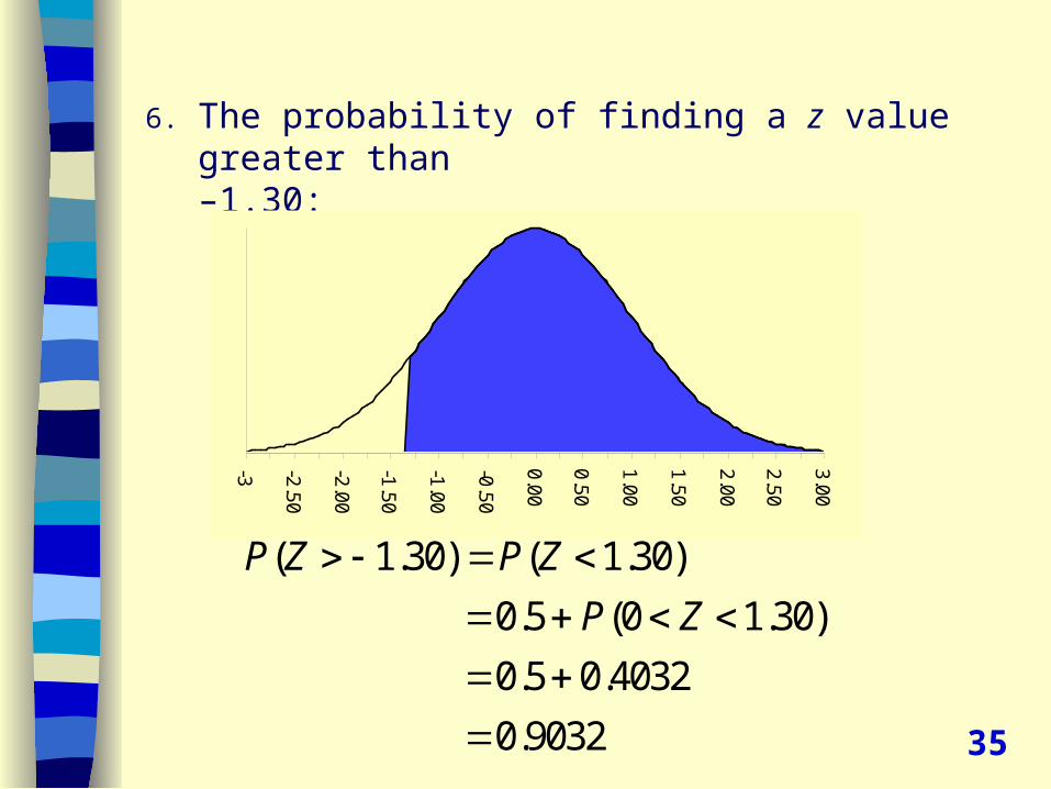
6. The probability of finding a z value greater than –1.30:

-3 -2.50

-2.00

-1.50

-1.00

-0.50

0.00

0.50

1.00

1.50

2.00

2.50

3.00

( 1.30) ( 1.30)

0.5 (0 1.30)

0.5 0.4032

0.9032

P Z P Z

P Z

35

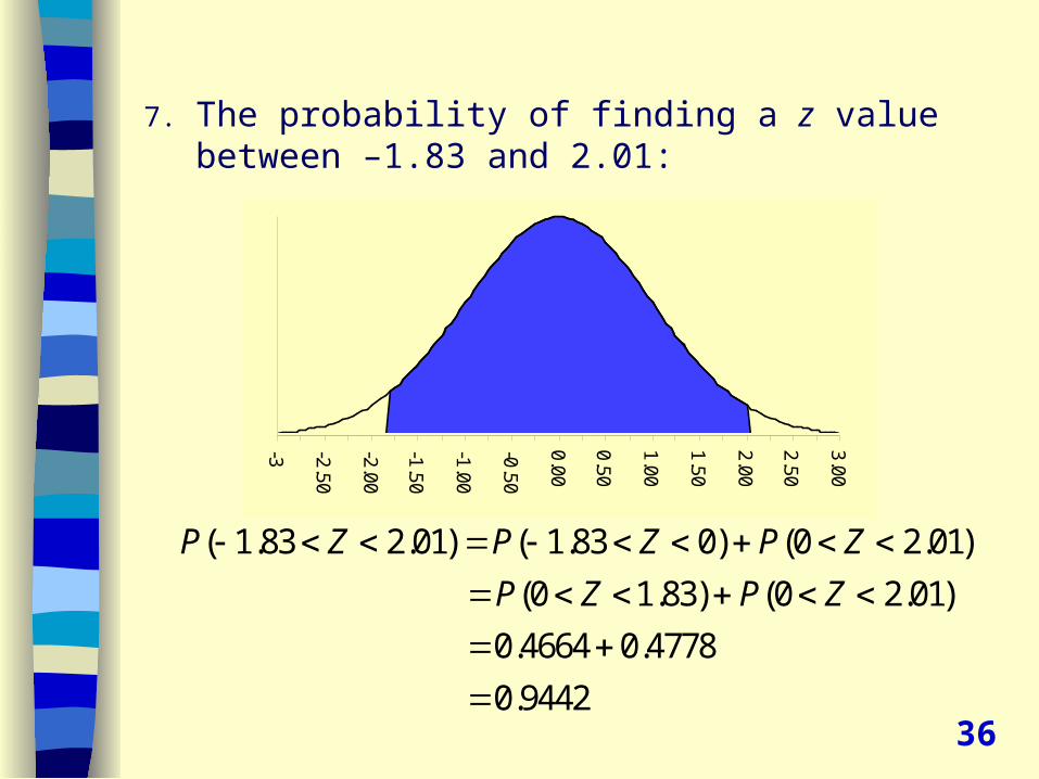
7. The probability of finding a z value between –1.83 and 2.01:

-3 -2.50

-2.00

-1.50

-1.00

-0.50

0.00

0.50

1.00

1.50

2.00

2.50

3.00

( 1.83 2.01) ( 1.83 0) (0 2.01)

(0 1.83) (0 2.01)

0.4664 0.4778

0.9442

P Z P Z P Z

P Z P Z

36

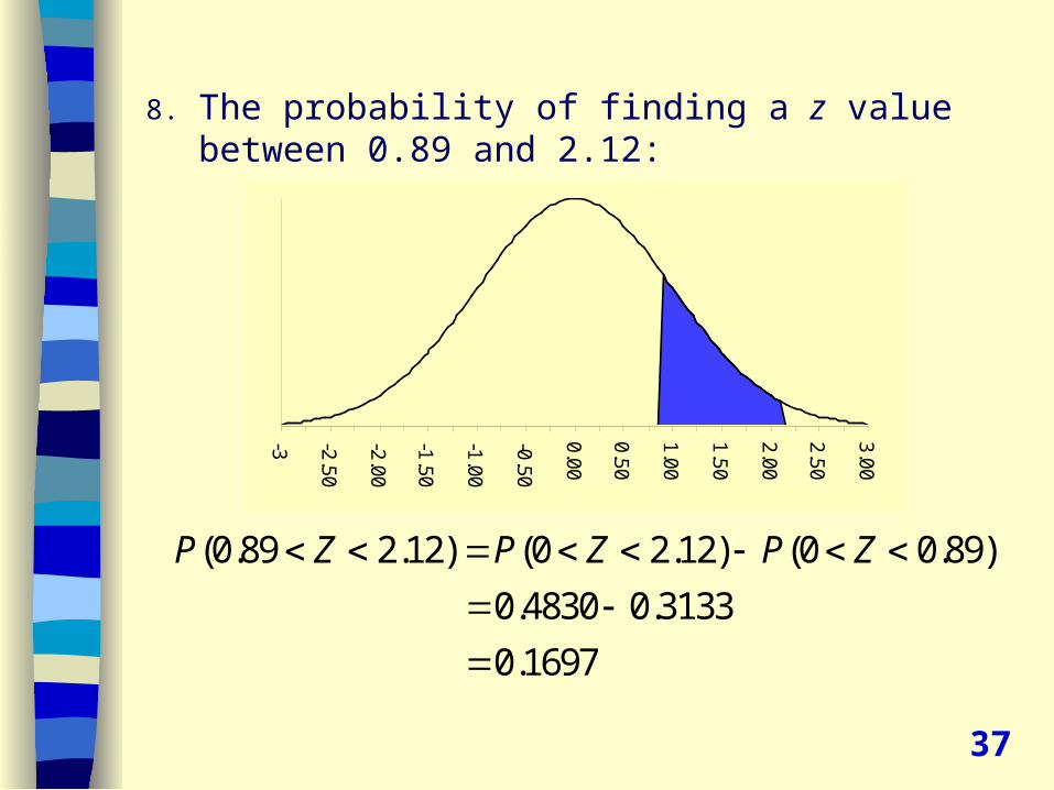
8. The probability of finding a z value between 0.89 and 2.12:

-3 -2.50

-2.00

-1.50

-1.00

-0.50

0.00

0.50

1.00

1.50

2.00

2.50

3.00

(0.89 2.12) (0 2.12) (0 0.89)

0.4830 0.3133

0.1697

P Z P Z P Z

37

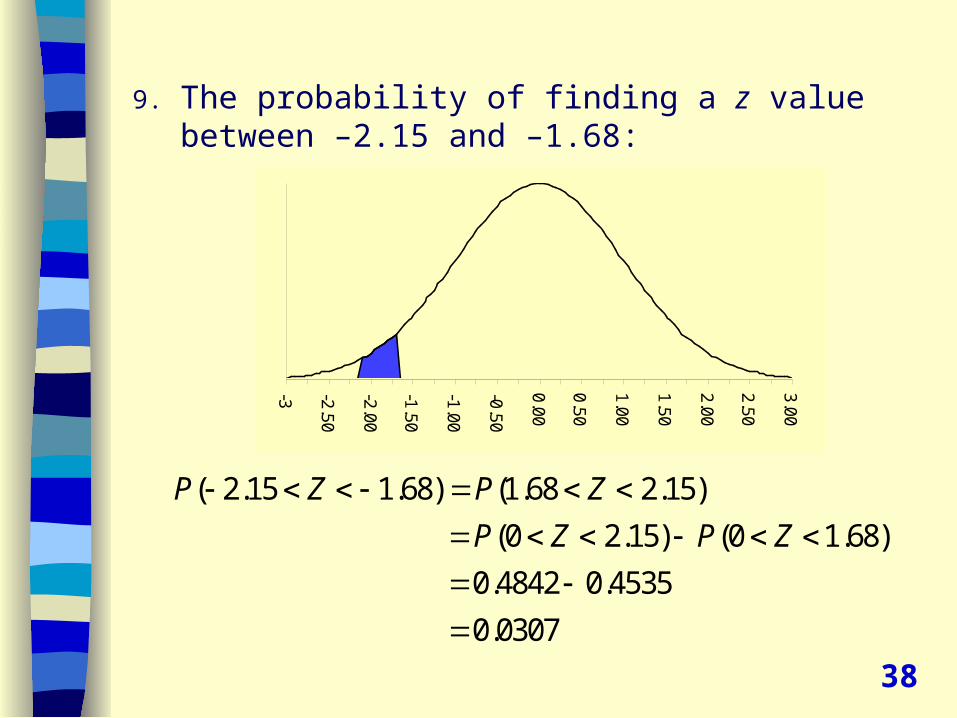
9. The probability of finding a z value between –2.15 and –1.68:

-3 -2.50

-2.00

-1.50

-1.00

-0.50

0.00

0.50

1.00

1.50

2.00

2.50

3.00

( 2.15 1.68) (1.68 2.15)

(0 2.15) (0 1.68)

0.4842 0.4535

0.0307

P Z P Z

P Z P Z

38

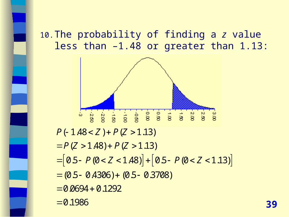
10. The probability of finding a z value less than –1.48 or greater than 1.13:

( 1.48 ) ( 1.13)

( 1.48) ( 1.13)

0.5 (0 1.48) 0.5 (0 1.13)

(0.5 0.4306) (0.5 0.3708)

0.0694 0.1292

0.1986

P Z P Z

P Z P Z

P Z P Z

39

Reading for next lecture

• Chapter 5, reread section 5.7

Exercises

• 5.50• 5.51• 5.52

40