Primer on Analyzing Animal Sounds: Figures and Sample Sounds Jack Bradbury & Sandra Vehrencamp...
85
Primer on Analyzing Animal Sounds: Figures and Sample Sounds Jack Bradbury & Sandra Vehrencamp Cornell University
-
Upload
zachery-jardine -
Category
Documents
-
view
219 -
download
0
Transcript of Primer on Analyzing Animal Sounds: Figures and Sample Sounds Jack Bradbury & Sandra Vehrencamp...
Primer on Analyzing Animal Sounds:
Figures and Sample Sounds
Jack Bradbury & Sandra Vehrencamp
Cornell University
Recording Sounds• A sound is a propagated disturbance in the
ambient pressure of a medium (air, water, etc.)
• Each region of higher-than ambient pressure is matched by a following region of lower-than average pressure
• A microphone converts the variations in pressure created by a passing sound wave into electrical signals that mimic the rise and fall of sound pressure at the microphone
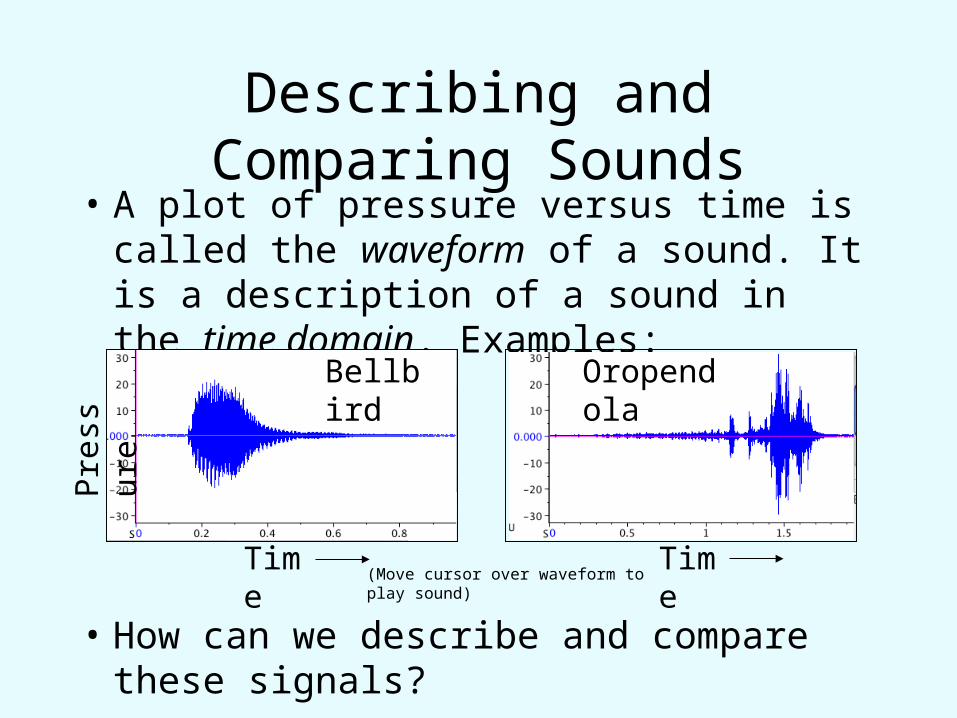
Describing and Comparing Sounds• A plot of pressure versus time is called the
waveform of a sound. It is a description of a sound in the time domain. Examples:
• How can we describe and compare these signals?
Pre
ssur
e
Time Time
Bellbird Oropendola
(Move cursor over waveform to play sound)

Simple Waveforms• The simplest type of signal one could ever
record is a single sine wave that does not change in either amplitude or frequency:
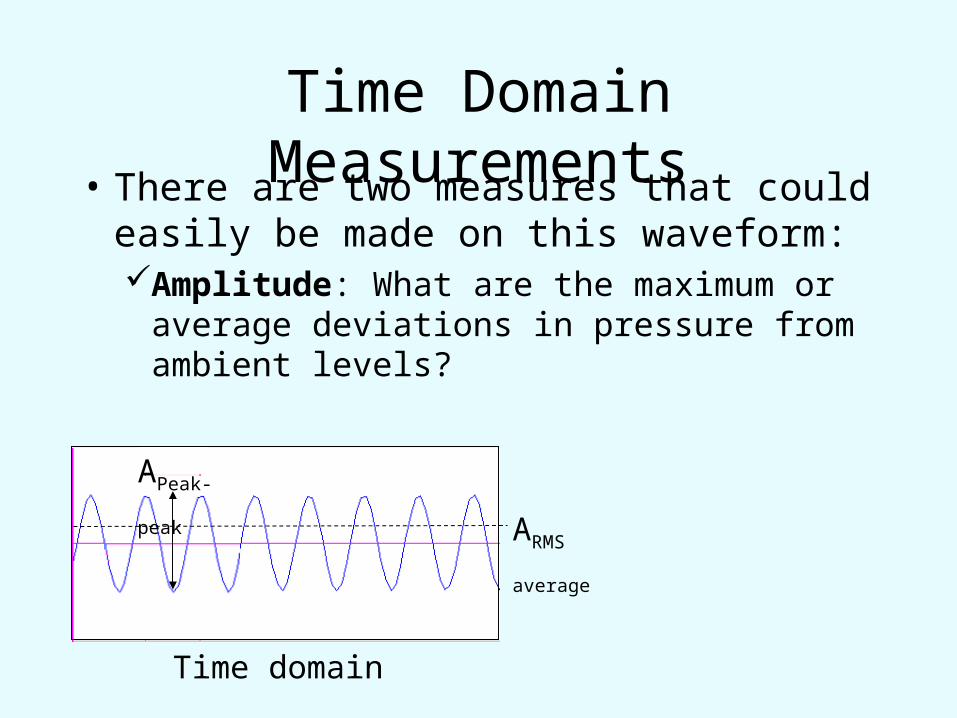
Time Domain Measurements• There are two measures that could easily be
made on this waveform:Amplitude: What are the maximum or average
deviations in pressure from ambient levels?
Time domain
APeak-peak
ARMS average
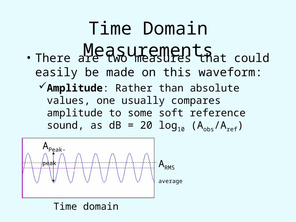
Time Domain Measurements• There are two measures that could easily be
made on this waveform:Amplitude: Rather than absolute values, one
usually compares amplitude to some soft reference sound, as dB = 20 log10 (Aobs/Aref)
Time domain
APeak-peak
ARMS average
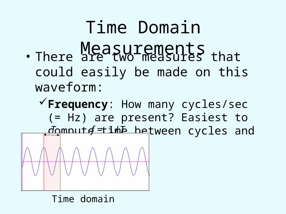
Time Domain Measurements• There are two measures that could easily be
made on this waveform:Frequency: How many cycles/sec (= Hz) are
present? Easiest to compute time between cycles and take reciprocalT
Time domain
f = 1/T
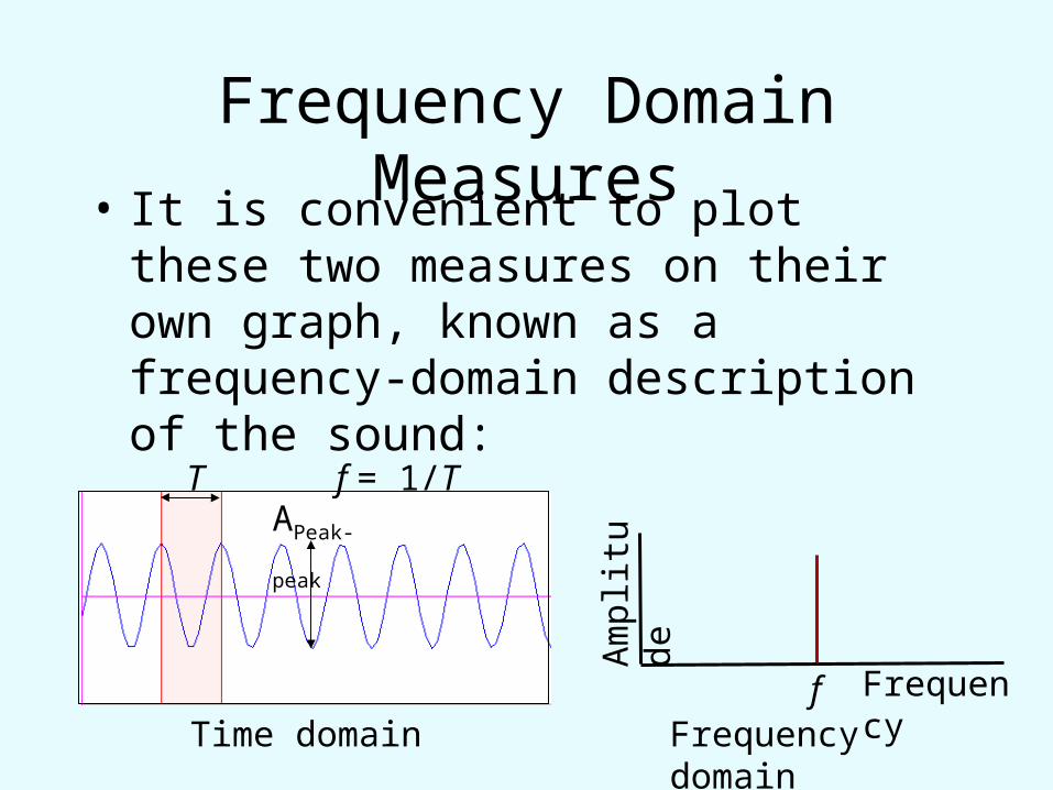
Frequency Domain Measures• It is convenient to plot these two measures
on their own graph, known as a frequency-domain description of the sound:
Am
plit
ude
Frequency
T
Time domain Frequency domain
f = 1/T
f
APeak-peak
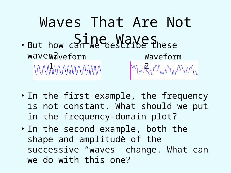
Waves That Are Not Sine Waves• But how can we describe these waves?
• In the first example, the frequency is not constant. What should we put in the frequency-domain plot?
• In the second example, both the shape and amplitude of the successive “waves” change. What can we do with this one?
Waveform 1 Waveform 2
Fourier Analysis• There is hope!
Any continuous waveform can be broken down into a set of pure sine waves with frequency and amplitude values that can be computed or measured (Fourier analysis).
Frequency-domain plots provide us with a very powerful way to describe and compare any set of sounds.
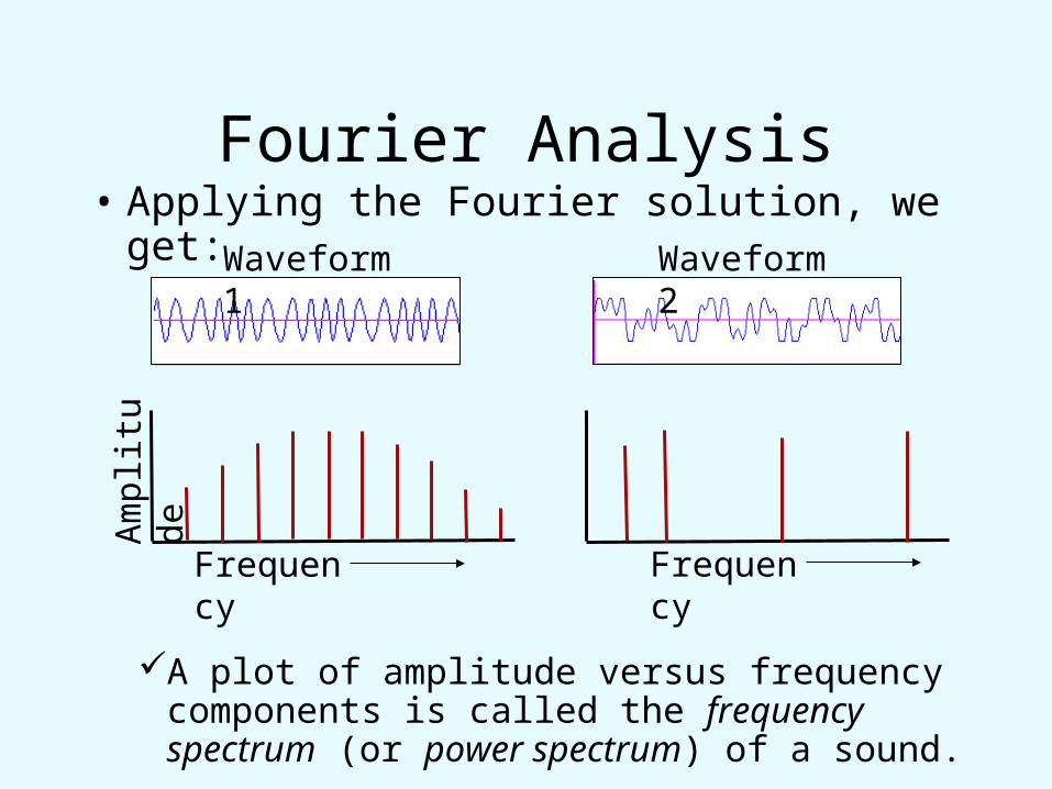
Fourier Analysis• Applying the Fourier solution, we get:
A plot of amplitude versus frequency components is called the frequency spectrum (or power spectrum) of a sound.
Am
plit
ude
Frequency Frequency
Waveform 1 Waveform 2

Fourier Analysis• But what do we do if the waveform keeps
changing during the signal, like in this lark sparrow song?
Pre
ssur
e
Time
(Move cursor over waveform to play sound)

Fourier Analysis• But what do we do if the waveform keeps
changing during the signal, like in this lark sparrow song?
• The solution is to break the song into homogeneous segments and create a frequency spectrum for each segment.
Pre
ssur
e
Time
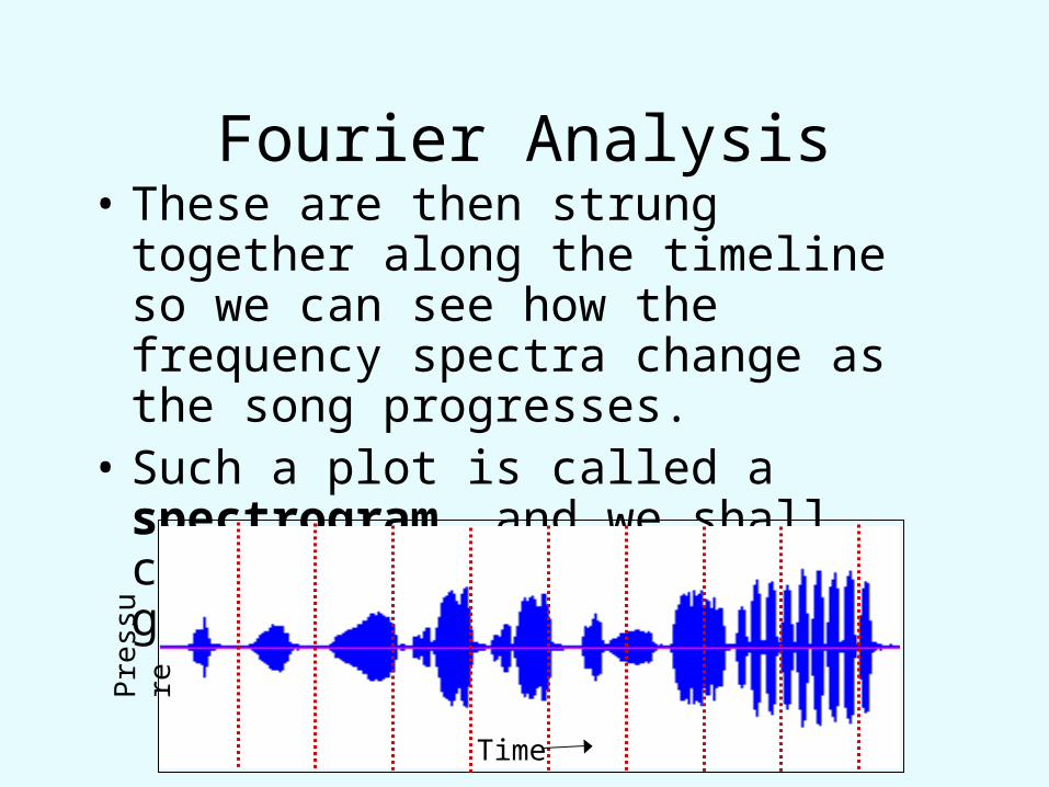
Fourier Analysis• These are then strung together along the
timeline so we can see how the frequency spectra change as the song progresses.
• Such a plot is called a spectrogram, and we shall come back to how these are generated.
Pre
ssur
e
Time
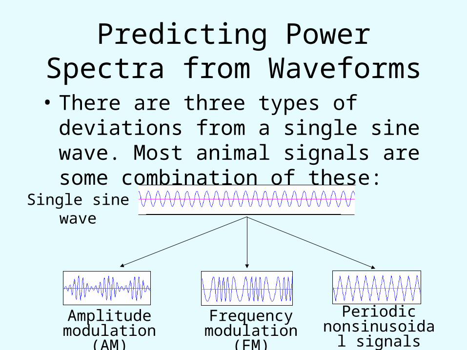
Predicting Power Spectra from Waveforms
• There are three types of deviations from a single sine wave. Most animal signals are some combination of these:
Single sine wave
Amplitude modulation (AM)
Frequency modulation (FM)
Periodic nonsinusoidal
signals

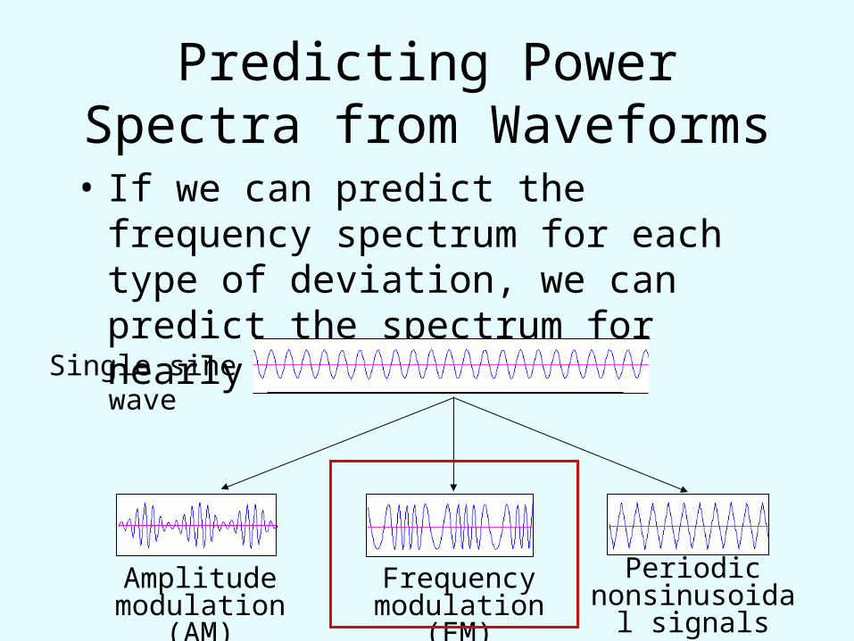
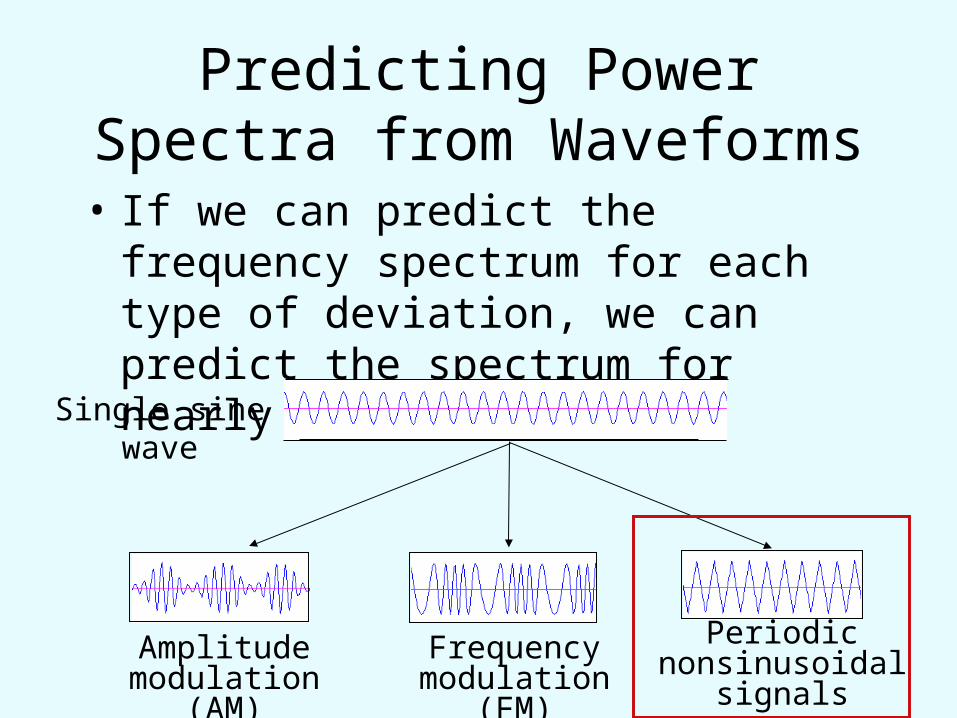
Predicting Power Spectra from Waveforms
• If we can predict the frequency spectrum for each type of deviation, we can predict the spectrum for nearly any signal.
Single sine wave
Amplitude modulation (AM)
Frequency modulation (FM)
Periodic nonsinusoidal
signals
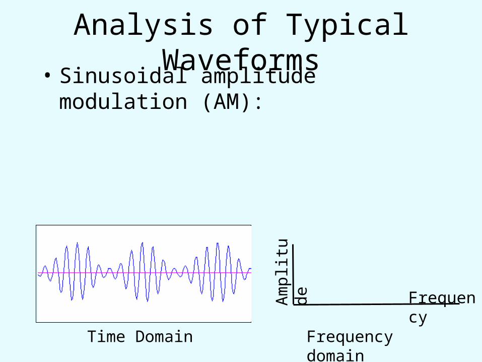
Analysis of Typical Waveforms• Sinusoidal amplitude modulation (AM):
Am
plit
ude
Frequency
Time Domain Frequency domain
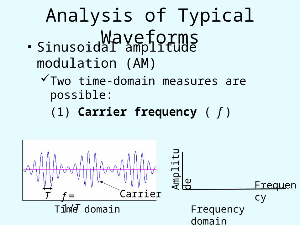
Analysis of Typical Waveforms• Sinusoidal amplitude modulation (AM)
Two time-domain measures are possible:
(1) Carrier frequency ( f )
Am
plit
ude
Frequency
Time domain Frequency domainT f = 1/T Carrier
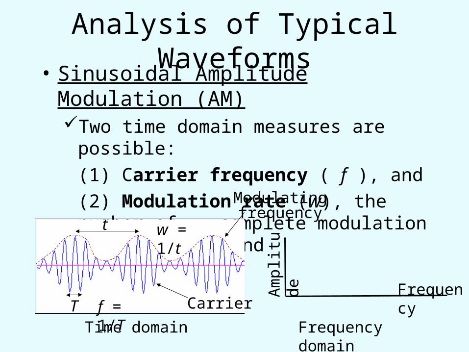
Analysis of Typical Waveforms• Sinusoidal Amplitude Modulation (AM)
Two time domain measures are possible:
(1) Carrier frequency ( f ), and
(2) Modulation rate (w), the number of complete modulation cycles per second
Am
plit
ude
Frequency
Time domain Frequency domainT f = 1/T
t w = 1/t
Carrier
Modulating frequency
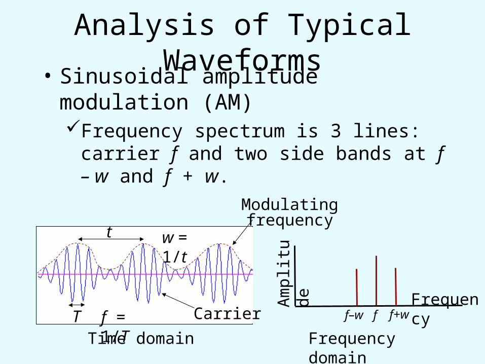
Analysis of Typical Waveforms• Sinusoidal amplitude modulation (AM)
Frequency spectrum is 3 lines: carrier f and two side bands at f – w and f + w.
Am
plit
ude
Frequency
Time domain Frequency domain
fT f = 1/T
t w = 1/t
f–w f+wCarrier
Modulating frequency
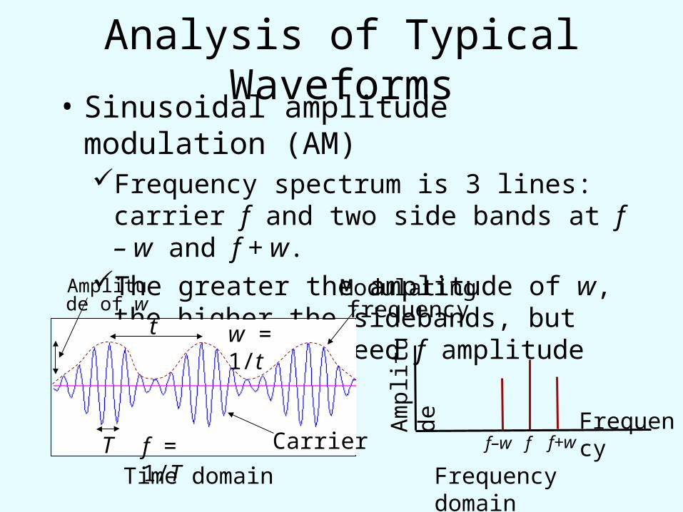
Analysis of Typical Waveforms• Sinusoidal amplitude modulation (AM)
Frequency spectrum is 3 lines: carrier f and two side bands at f – w and f + w.
The greater the amplitude of w, the higher the sidebands, but these never exceed f amplitude
Am
plit
ude
Frequency
Time domain Frequency domain
fT f = 1/T
t w = 1/t
f–w f+wCarrier
Modulating frequency
Amplitude of w
Predicting Power Spectra from Waveforms
• If we can predict the frequency spectrum for each type of deviation, we can predict the spectrum for nearly any signal.
Single sine wave
Amplitude modulation (AM)
Frequency modulation (FM)
Periodic nonsinusoidal
signals
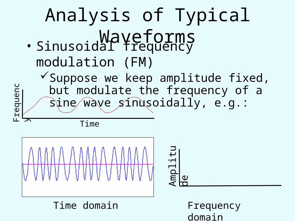
Analysis of Typical Waveforms• Sinusoidal frequency modulation (FM)
Suppose we keep amplitude fixed, but modulate the frequency of a sine wave sinusoidally, e.g.:
Am
plit
ude
Time domain Frequency domain
Fre
quen
cy
Time
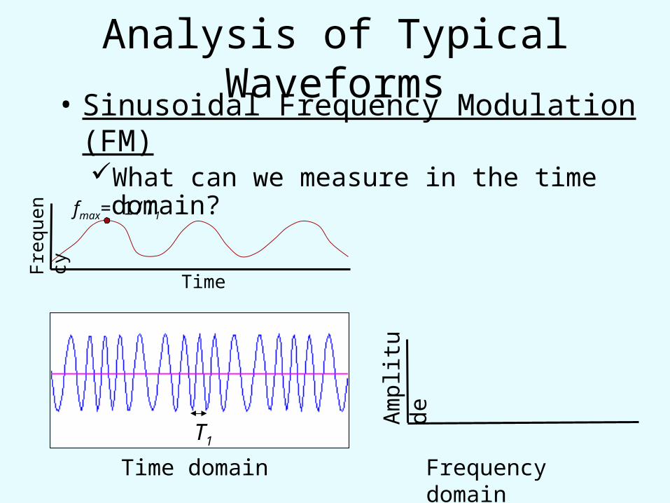
Analysis of Typical Waveforms• Sinusoidal Frequency Modulation (FM)
What can we measure in the time domain?
Am
plit
ude
Time domain Frequency domain
Fre
quen
cy
Time
T1
fmax= 1/T1
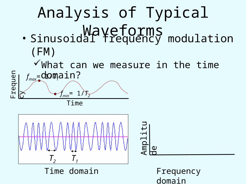
Analysis of Typical Waveforms• Sinusoidal frequency modulation (FM)
What can we measure in the time domain?
Am
plit
ude
Time domain Frequency domain
Fre
quen
cy
Time
T2 T1
fmax= 1/T1
fmin= 1/T2
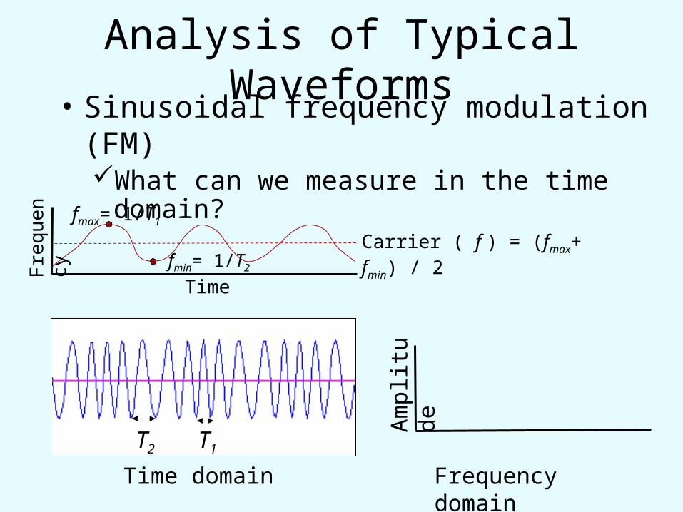
Analysis of Typical Waveforms• Sinusoidal frequency modulation (FM)
What can we measure in the time domain?
Am
plit
ude
Time domain Frequency domain
Fre
quen
cy
Time
T2 T1
fmax= 1/T1
fmin= 1/T2
Carrier ( f ) = (fmax+ fmin) / 2
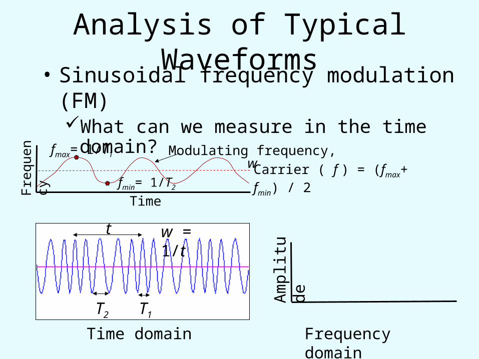
Analysis of Typical Waveforms• Sinusoidal frequency modulation (FM)
What can we measure in the time domain?
Am
plit
ude
Time domain Frequency domain
Modulating frequency, w
Fre
quen
cy
Time
T2 T1
fmax= 1/T1
fmin= 1/T2
t w = 1/t
Carrier ( f ) = (fmax+ fmin) / 2
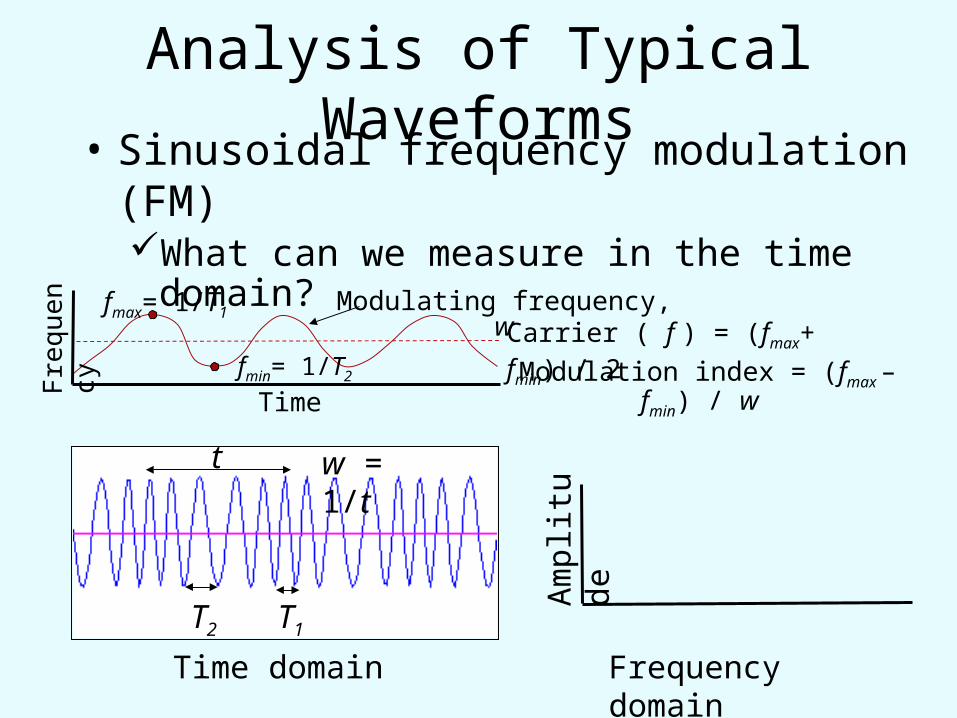
Analysis of Typical Waveforms• Sinusoidal frequency modulation (FM)
What can we measure in the time domain?
Am
plit
ude
Time domain Frequency domain
Modulating frequency, w
Fre
quen
cy
Time
T2 T1
fmax= 1/T1
fmin= 1/T2
t w = 1/t
Modulation index = (fmax – fmin) / w
Carrier ( f ) = (fmax+ fmin) / 2
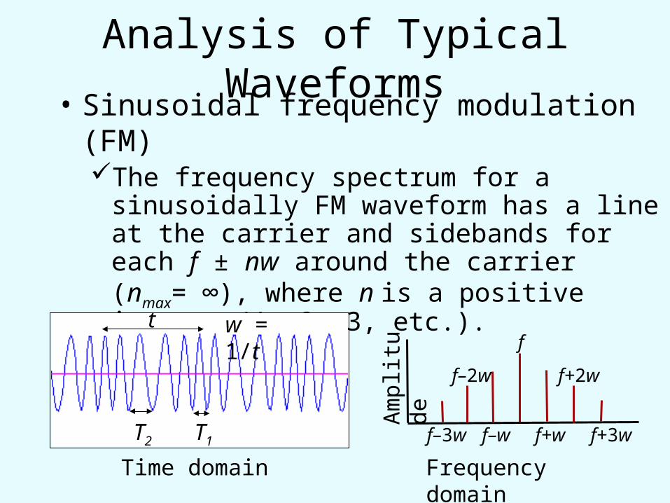
Analysis of Typical Waveforms• Sinusoidal frequency modulation (FM)
The frequency spectrum for a sinusoidally FM waveform has a line at the carrier and sidebands for each f ± nw around the carrier (nmax= ∞), where n is a positive integer (1, 2, 3, etc.).
Am
plit
ude
Time domain Frequency domain
f
f–w f+wT2 T1
t w = 1/t
f–2w
f–3w
f+2w
f+3w
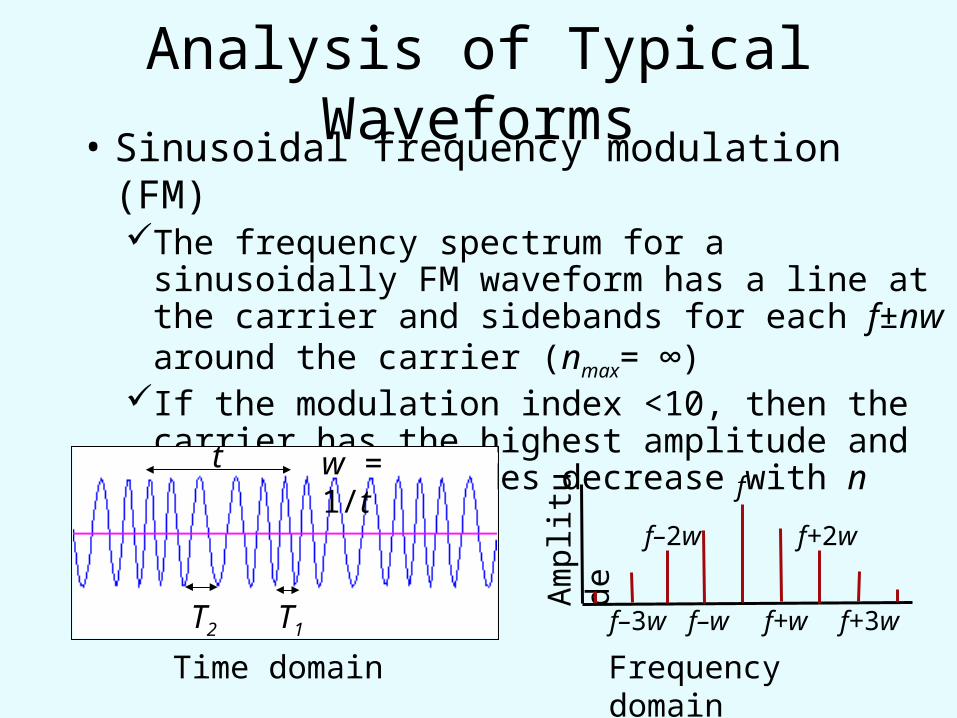
Analysis of Typical Waveforms• Sinusoidal frequency modulation (FM)
The frequency spectrum for a sinusoidally FM waveform has a line at the carrier and sidebands for each f±nw around the carrier (nmax= ∞)
If the modulation index <10, then the carrier has the highest amplitude and sideband amplitudes decrease with n
Am
plit
ude
Time domain Frequency domain
f
f–w f+wT2 T1
t w = 1/t
f–2w
f–3w
f+2w
f+3w
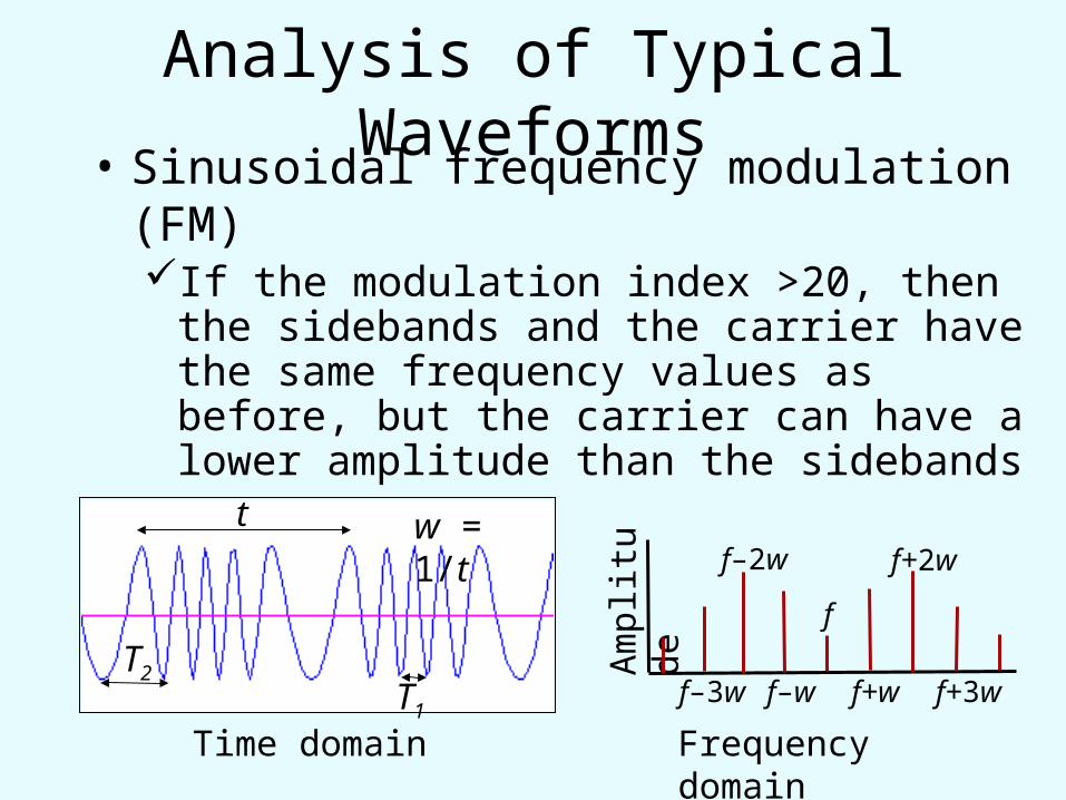
Analysis of Typical Waveforms• Sinusoidal frequency modulation (FM)
If the modulation index >20, then the sidebands and the carrier have the same frequency values as before, but the carrier can have a lower amplitude than the sidebands
Am
plit
ude
Time domain Frequency domain
f
f–w f+w
f–2w
f–3w
f+2w
f+3wT2
T1
t w = 1/t
Predicting Power Spectra from Waveforms
• If we can predict the frequency spectrum for each type of deviation, we can predict the spectrum for nearly any signal.
Single sine wave
Amplitude modulation (AM)
Frequency modulation (FM)
Periodic nonsinusoidal
signals
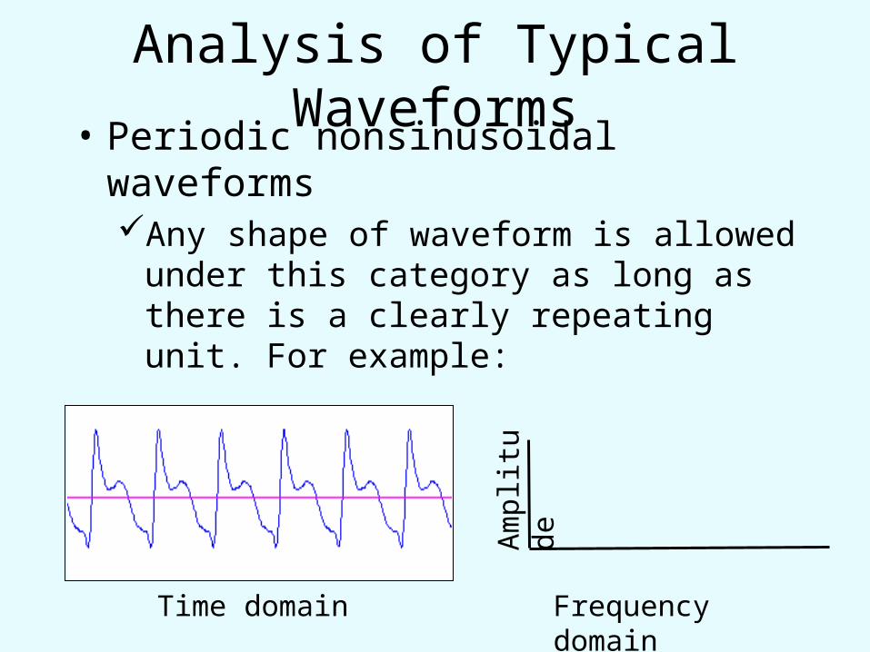
Analysis of Typical Waveforms• Periodic nonsinusoidal waveforms
Any shape of waveform is allowed under this category as long as there is a clearly repeating unit. For example:
Am
plit
ude
Time domain Frequency domain
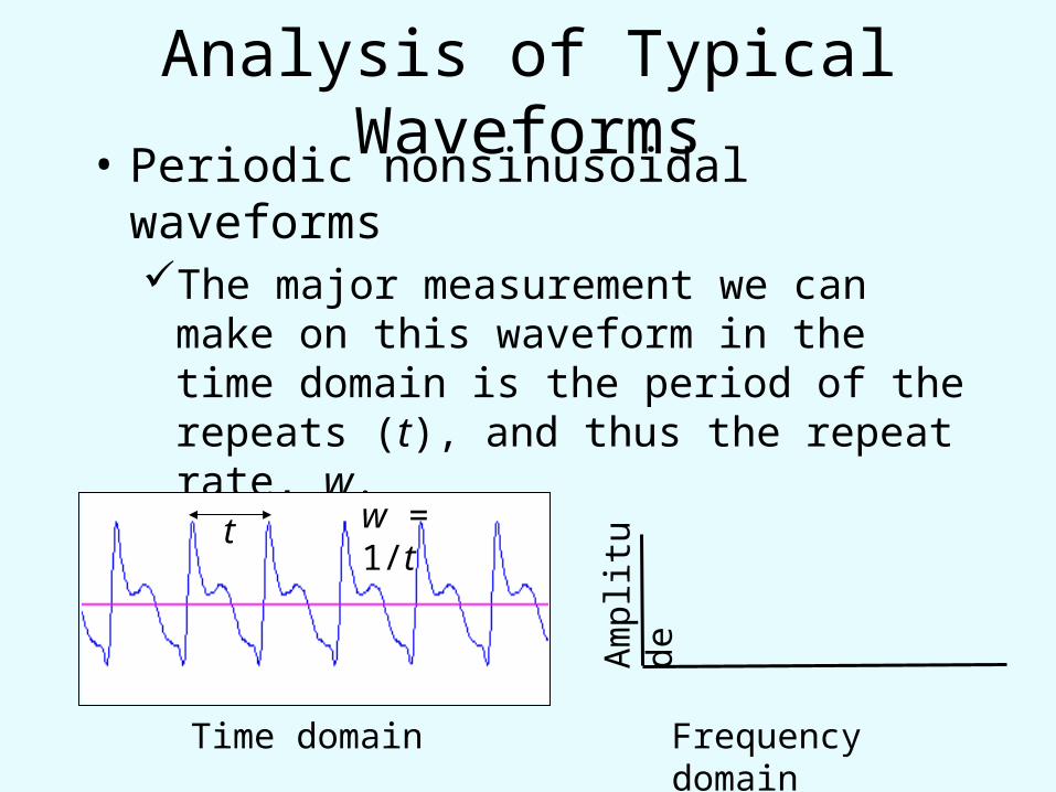
Analysis of Typical Waveforms• Periodic nonsinusoidal waveforms
The major measurement we can make on this waveform in the time domain is the period of the repeats (t), and thus the repeat rate, w.
Am
plit
ude
Time domain Frequency domain
t w = 1/t
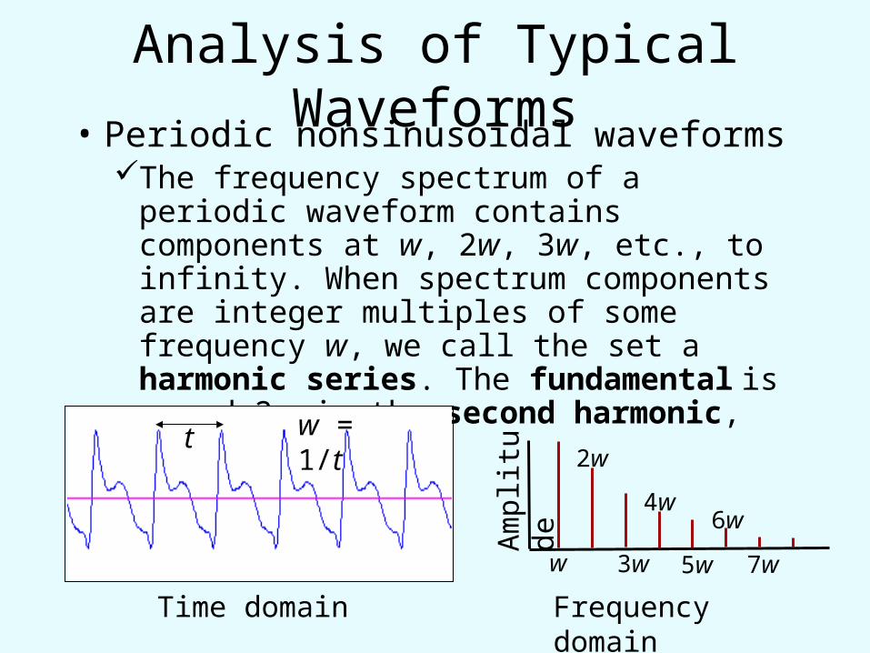
Analysis of Typical Waveforms• Periodic nonsinusoidal waveforms
The frequency spectrum of a periodic waveform contains components at w, 2w, 3w, etc., to infinity. When spectrum components are integer multiples of some frequency w, we call the set a harmonic series. The fundamental is w and 2w is the second harmonic, etc.
Am
plit
ude
Time domain Frequency domain
2w
w 3w 5w
4w6w
7w
t w = 1/t
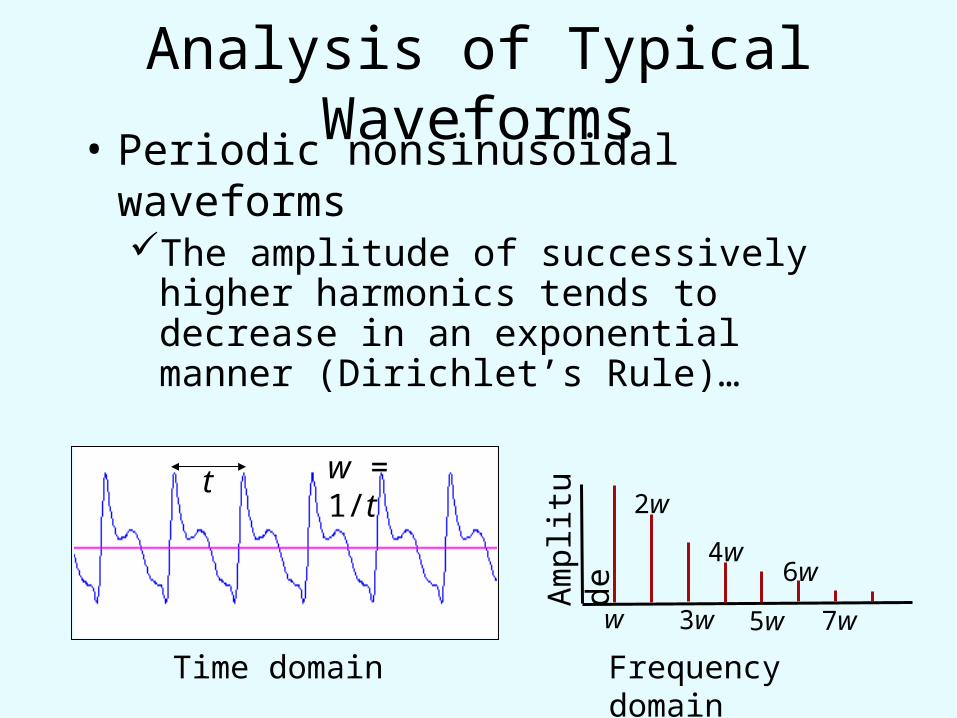
Analysis of Typical Waveforms• Periodic nonsinusoidal waveforms
The amplitude of successively higher harmonics tends to decrease in an exponential manner (Dirichlet’s Rule)…
Am
plit
ude
Time domain Frequency domain
2w
w 3w 5w
4w6w
7w
t w = 1/t
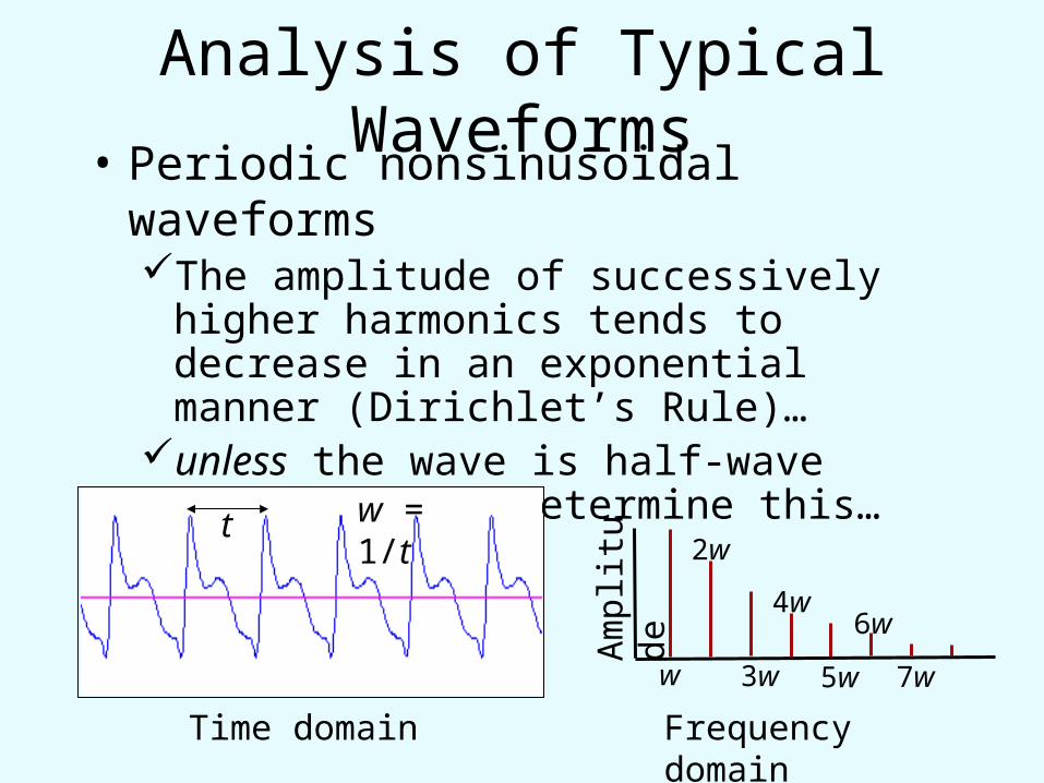
Analysis of Typical Waveforms• Periodic nonsinusoidal waveforms
The amplitude of successively higher harmonics tends to decrease in an exponential manner (Dirichlet’s Rule)…
unless the wave is half-wave symmetric. To determine this…
Am
plit
ude
Time domain Frequency domain
2w
w 3w 5w
4w6w
7w
t w = 1/t
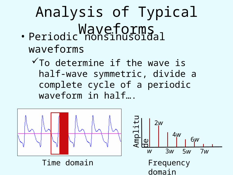
Analysis of Typical Waveforms• Periodic nonsinusoidal waveforms
To determine if the wave is half-wave symmetric, divide a complete cycle of a periodic waveform in half….
Am
plit
ude
Time domain Frequency domain
2w
w 3w 5w
4w6w
7w
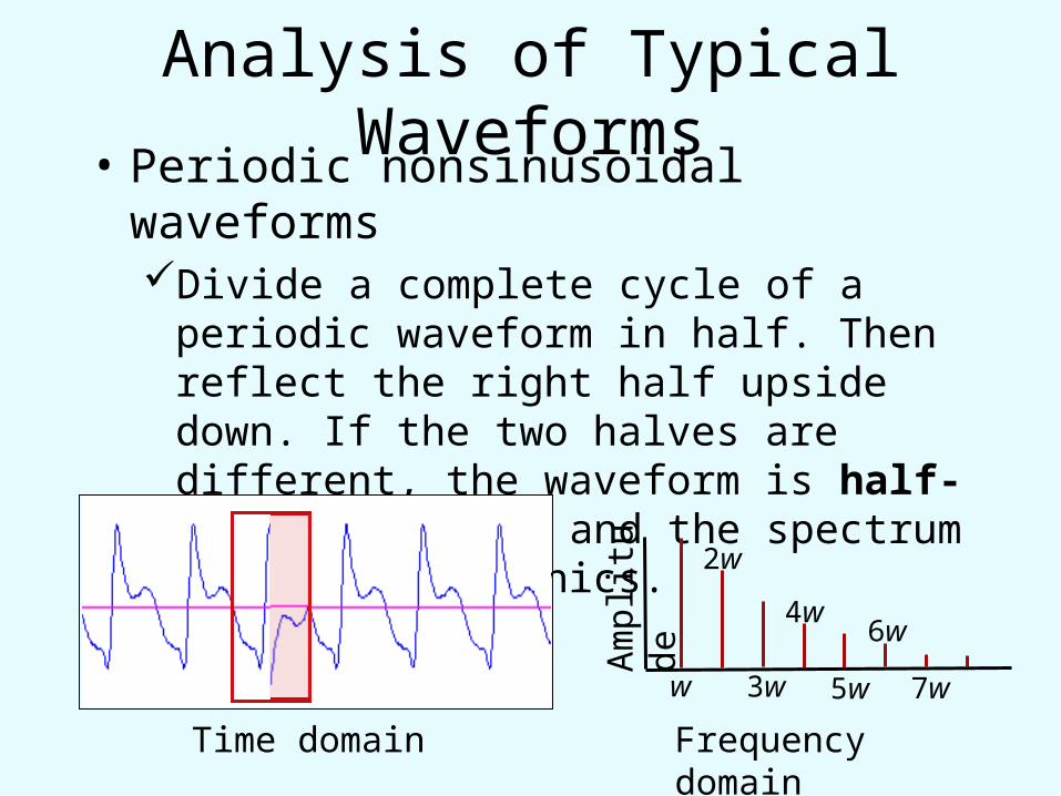
Analysis of Typical Waveforms• Periodic nonsinusoidal waveforms
Divide a complete cycle of a periodic waveform in half. Then reflect the right half upside down. If the two halves are different, the waveform is half-wave asymmetric and the spectrum shows all harmonics.
Am
plit
ude
Time domain Frequency domain
2w
w 3w 5w
4w6w
7w
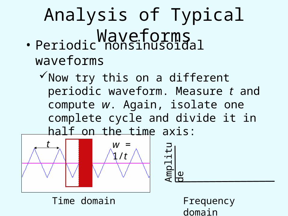
Analysis of Typical Waveforms• Periodic nonsinusoidal waveforms
Now try this on a different periodic waveform. Measure t and compute w. Again, isolate one complete cycle and divide it in half on the time axis:
Am
plit
ude
Time domain Frequency domain
t w = 1/t

Analysis of Typical Waveforms• Periodic nonsinusoidal waveforms
Now flip the right half upside down. If the two halves are the same, the waveform is half-wave symmetric and the amplitudes of all even harmonics are zero. Only odd harmonics are present to follow Dirichlet’s Rule.
Am
plit
ude
Time domain Frequency domain
w 3w 5w 7w
t w = 1/t
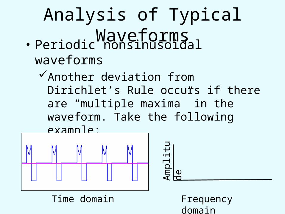
Analysis of Typical Waveforms• Periodic nonsinusoidal waveforms
Another deviation from Dirichlet’s Rule occurs if there are “multiple maxima” in the waveform. Take the following example:
Am
plit
ude
Time domain Frequency domain
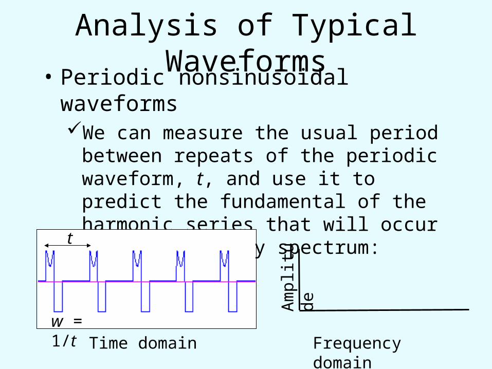
Analysis of Typical Waveforms• Periodic nonsinusoidal waveforms
We can measure the usual period between repeats of the periodic waveform, t, and use it to predict the fundamental of the harmonic series that will occur in the frequency spectrum:
Am
plit
ude
Time domain Frequency domain
t
w = 1/t
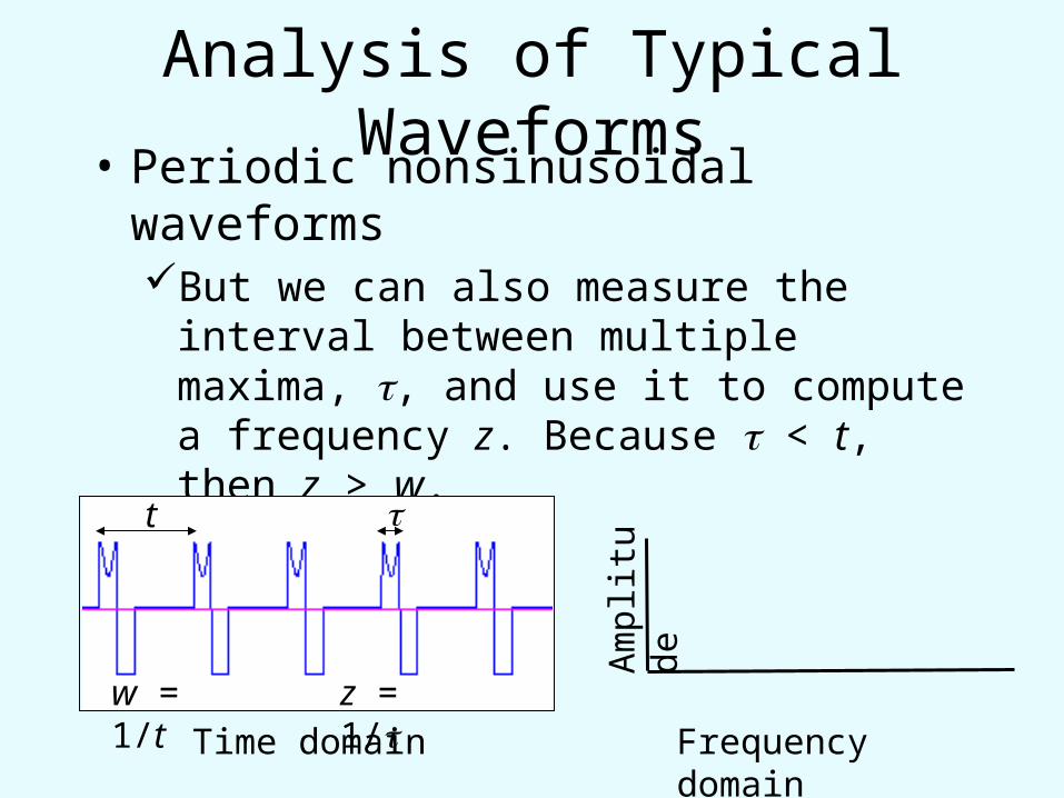
Analysis of Typical Waveforms• Periodic nonsinusoidal waveforms
But we can also measure the interval between multiple maxima, , and use it to compute a frequency z. Because < t, then z > w.
Am
plit
ude
Time domain Frequency domain
t
w = 1/t
z = 1/
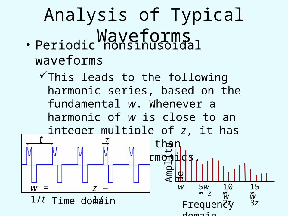
Analysis of Typical Waveforms• Periodic nonsinusoidal waveforms
This leads to the following harmonic series, based on the fundamental w. Whenever a harmonic of w is close to an integer multiple of z, it has lower amplitude than intermediate harmonics.
Am
plit
ude
Time domain Frequency domain
15ww 10w5w
t
w = 1/t
z = 1/≈ z ≈ 2z ≈ 3z
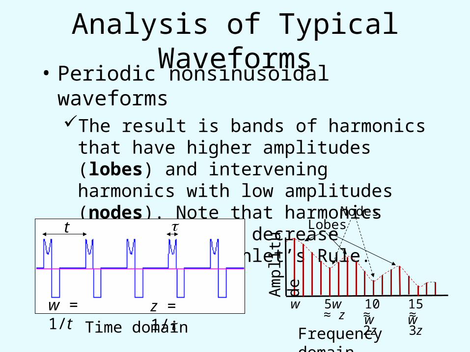
Analysis of Typical Waveforms• Periodic nonsinusoidal waveforms
The result is bands of harmonics that have higher amplitudes (lobes) and intervening harmonics with low amplitudes (nodes). Note that harmonics still gradually decrease following Dirichlet’s Rule.
Am
plit
ude
Time domain Frequency domain
15ww 10w5w
t
w = 1/t
z = 1/≈ z ≈ 2z ≈ 3z
LobesNodes
Analysis of Typical Waveforms• Compound waveforms
While a few birds can emit pure sine waves, most animal sounds are some combination of AM, FM, and/or nonsinusoidal periodic signals.
We call these compound waveforms.Compound waveforms can always be
decomposed into a set of carrier sine waves and a set of modulating sine waves. We can then use the simple rules of AM and FM to add the appropriate sidebands for each modulating sine wave around each carrier sine wave. This is the spectrum of the compound wave.
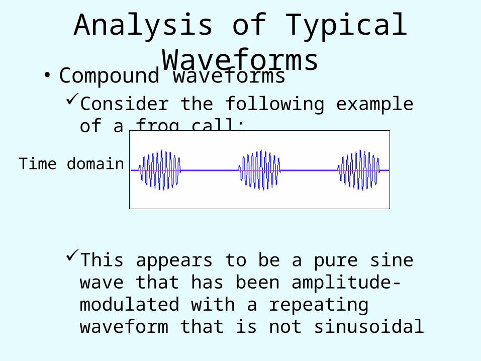
Analysis of Typical Waveforms• Compound waveforms
Consider the following example of a frog call:
This appears to be a pure sine wave that has been amplitude-modulated with a repeating waveform that is not sinusoidal
Time domain
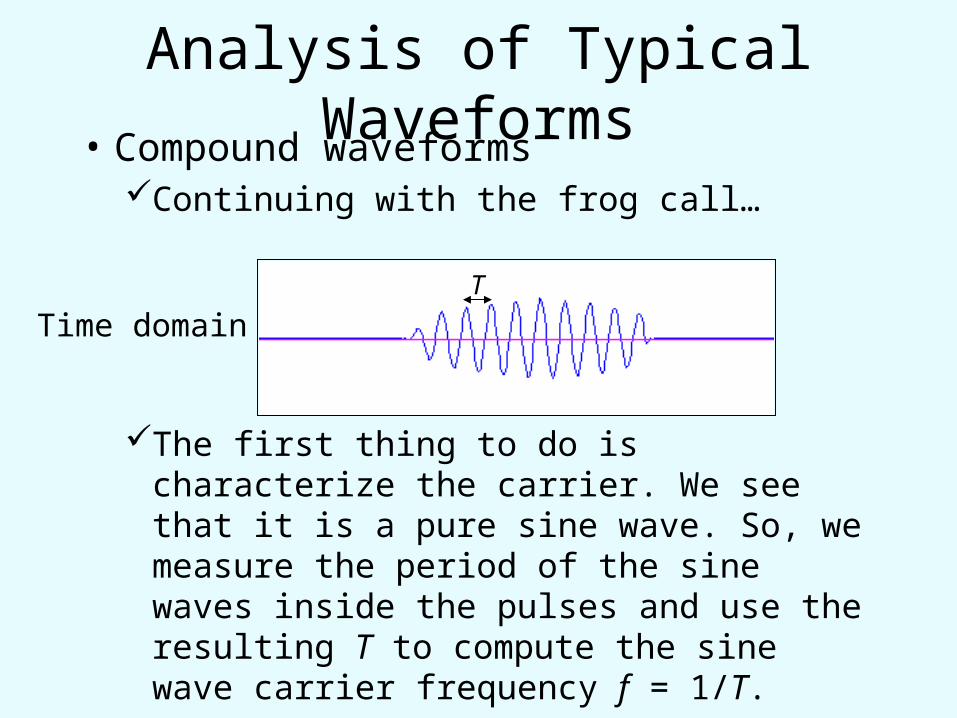
Analysis of Typical Waveforms• Compound waveforms
Continuing with the frog call…
The first thing to do is characterize the carrier. We see that it is a pure sine wave. So, we measure the period of the sine waves inside the pulses and use the resulting T to compute the sine wave carrier frequency f = 1/T.
Time domainT
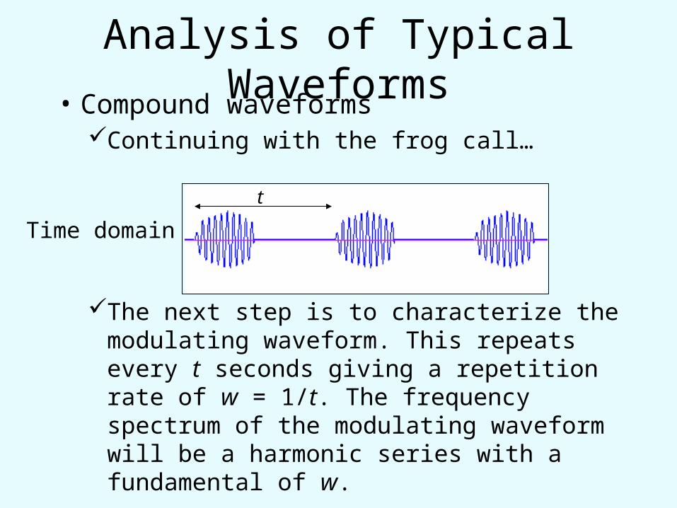
Analysis of Typical Waveforms• Compound waveforms
Continuing with the frog call…
The next step is to characterize the modulating waveform. This repeats every t seconds giving a repetition rate of w = 1/t. The frequency spectrum of the modulating waveform will be a harmonic series with a fundamental of w.
Time domain
t
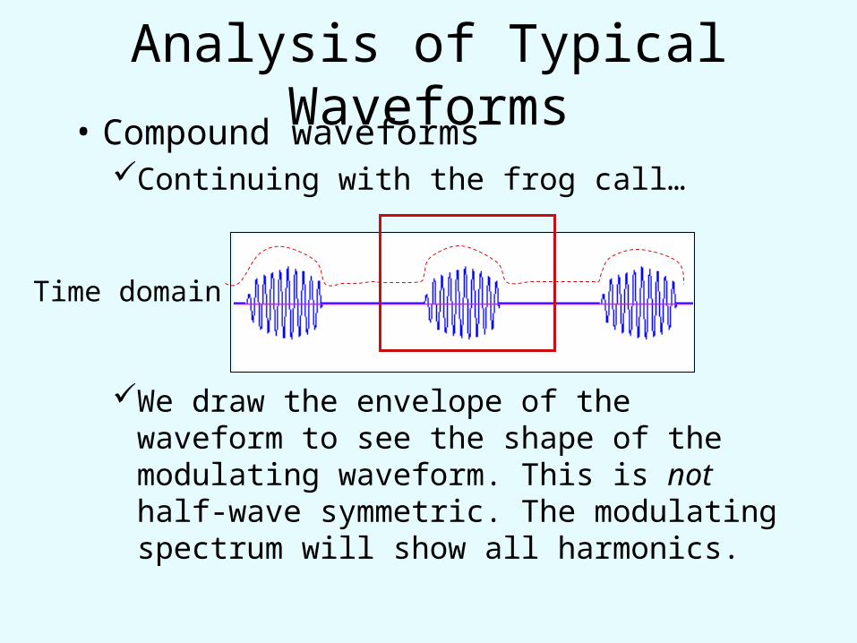
Analysis of Typical Waveforms• Compound waveforms
Continuing with the frog call…
We draw the envelope of the waveform to see the shape of the modulating waveform. This is not half-wave symmetric. The modulating spectrum will show all harmonics.
Time domain
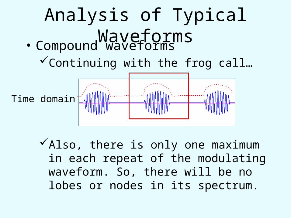
Analysis of Typical Waveforms• Compound waveforms
Continuing with the frog call…
Also, there is only one maximum in each repeat of the modulating waveform. So, there will be no lobes or nodes in its spectrum.
Time domain
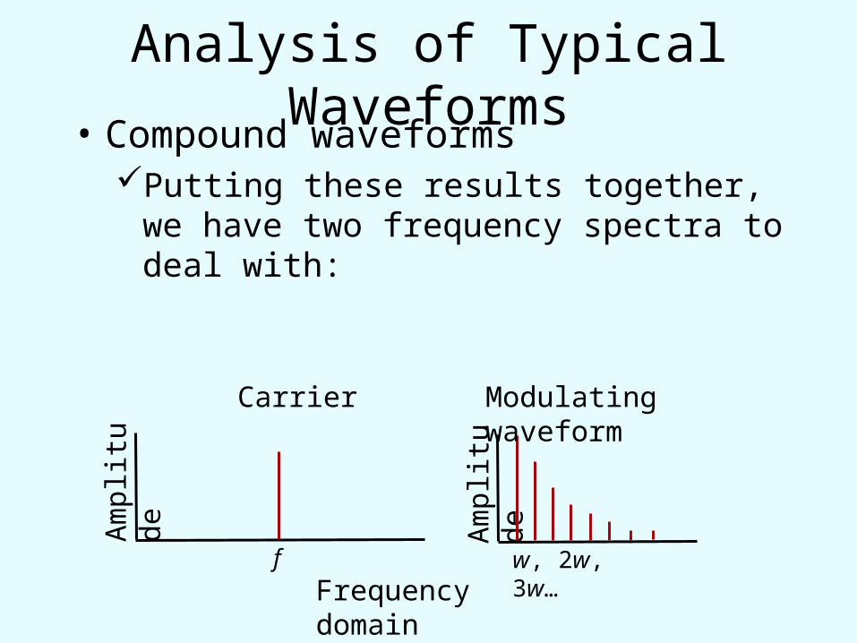
Analysis of Typical Waveforms• Compound waveforms
Putting these results together, we have two frequency spectra to deal with:
Am
plit
ude
Frequency domainf
Am
plit
ude
w, 2w, 3w…
Carrier Modulating waveform
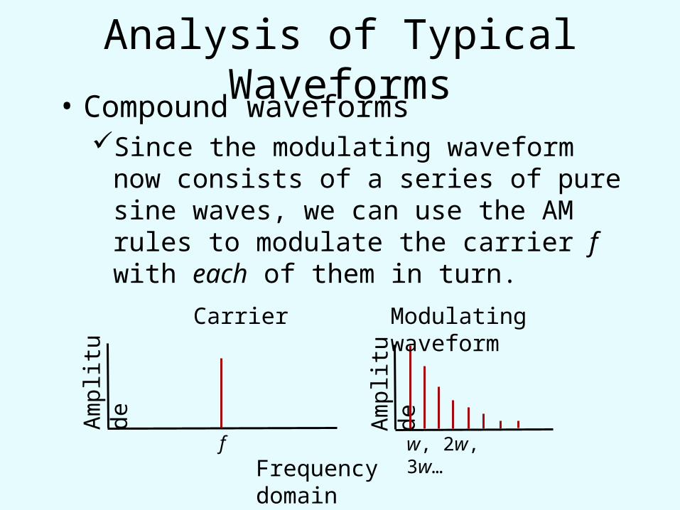
Analysis of Typical Waveforms• Compound waveforms
Since the modulating waveform now consists of a series of pure sine waves, we can use the AM rules to modulate the carrier f with each of them in turn.
Am
plit
ude
Frequency domainf
Am
plit
ude
w, 2w, 3w…
Carrier Modulating waveform
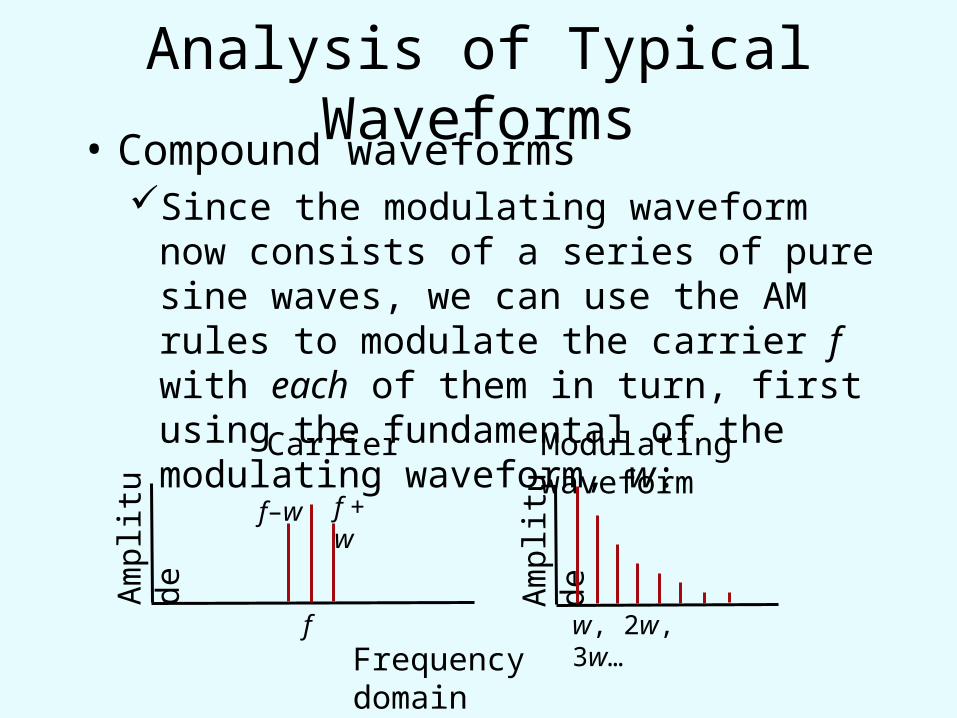
Analysis of Typical Waveforms• Compound waveforms
Since the modulating waveform now consists of a series of pure sine waves, we can use the AM rules to modulate the carrier f with each of them in turn, first using the fundamental of the modulating waveform, w:
Am
plit
ude
Frequency domainf
Am
plit
ude
w, 2w, 3w…
Carrier Modulating waveform
f + wf–w
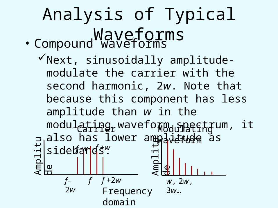
Analysis of Typical Waveforms• Compound waveforms
Next, sinusoidally amplitude-modulate the carrier with the second harmonic, 2w. Note that because this component has less amplitude than w in the modulating waveform spectrum, it also has lower amplitude as sidebands.
Am
plit
ude
Frequency domainf
Am
plit
ude
w, 2w, 3w…
Carrier Modulating waveform
f +wf–w
f–2w
f +2w
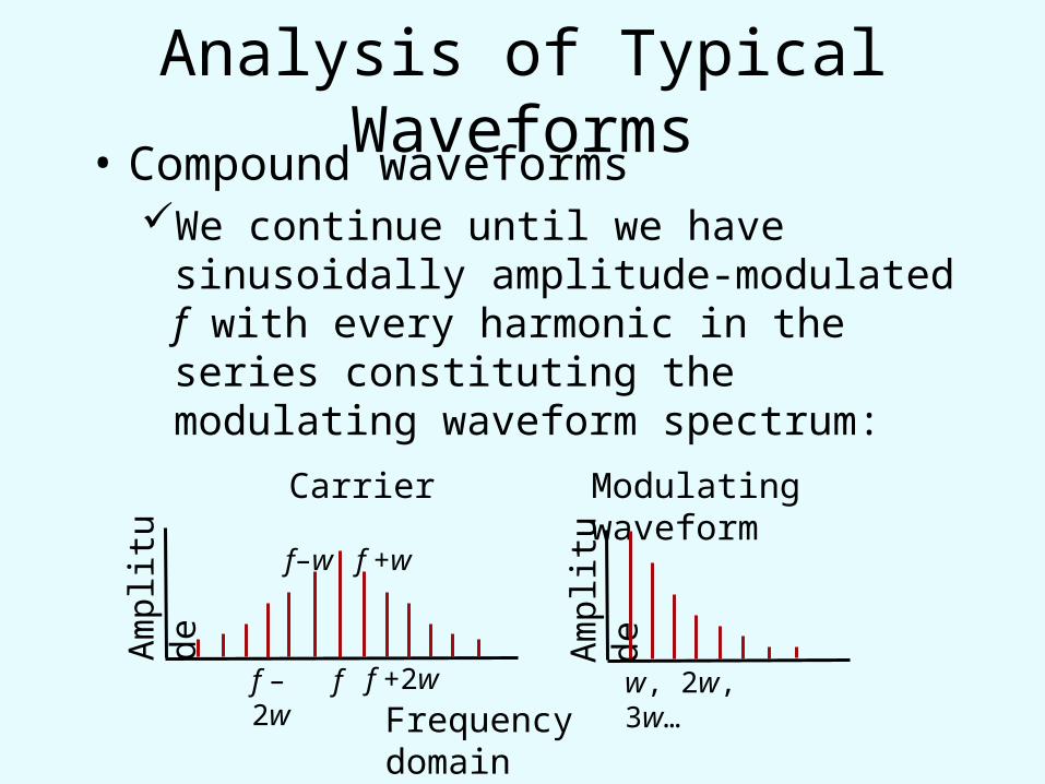
Analysis of Typical Waveforms• Compound waveforms
We continue until we have sinusoidally amplitude-modulated f with every harmonic in the series constituting the modulating waveform spectrum:
Am
plit
ude
Frequency domainf
Am
plit
ude
w, 2w, 3w…
Carrier Modulating waveform
f +wf–w
f –2w
f +2w
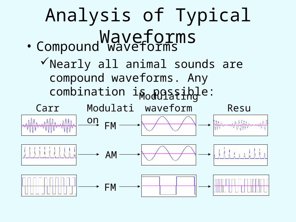
Analysis of Typical Waveforms• Compound waveforms
Nearly all animal sounds are compound waveforms. Any combination is possible:
Carrier ModulationModulating waveform Result
FM
AM
FM

The Uncertainty Principle
• Any Fourier analyzer needs several cycles of a signal to compute component frequencies.
• The more cycles of a stable frequency component that an analyzer can measure, the more accurate the measurement of that frequency.
Medium duration sample
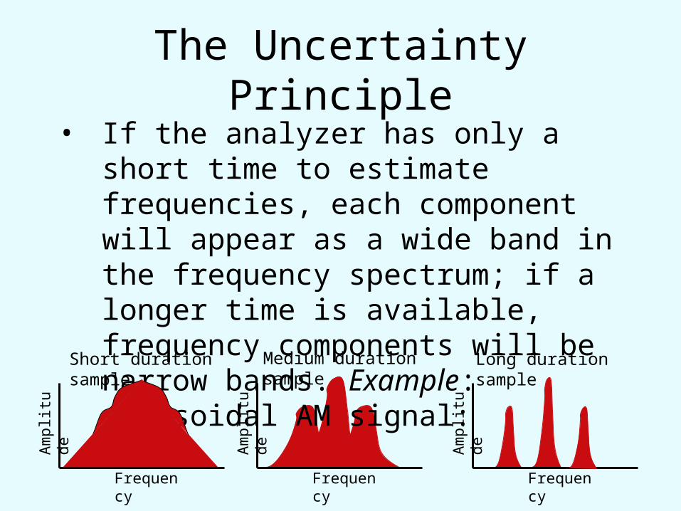
The Uncertainty Principle
• If the analyzer has only a short time to estimate frequencies, each component will appear as a wide band in the frequency spectrum; if a longer time is available, frequency components will be narrow bands. Example: sinusoidal AM signal:
Am
plit
ude
Frequency
Long duration sample
Am
plit
ude
Frequency
Am
plit
ude
Frequency
Short duration sample
Medium duration sample
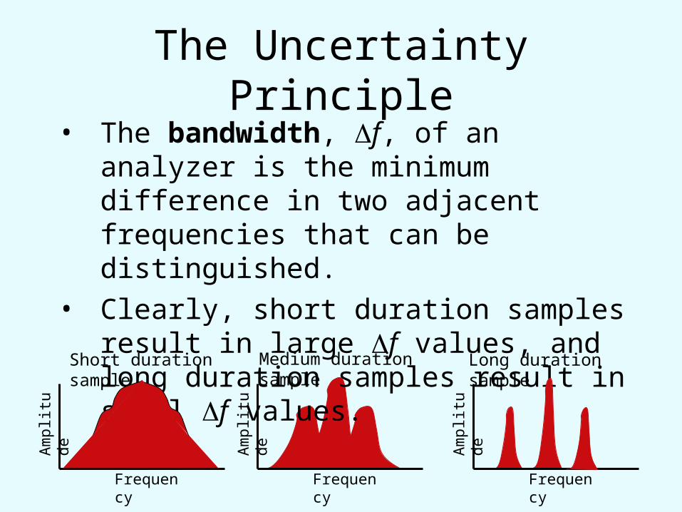
The Uncertainty Principle
• The bandwidth, f, of an analyzer is the minimum difference in two adjacent frequencies that can be distinguished.
• Clearly, short duration samples result in large f values, and long duration samples result in small f values.
Am
plit
ude
Frequency
Long duration sample
Am
plit
ude
Frequency
Am
plit
ude
Frequency
Short duration sample
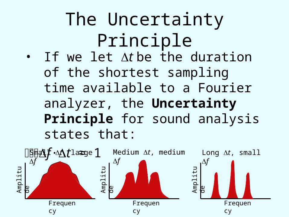
• If we let t be the duration of the shortest sampling time available to a Fourier analyzer, the Uncertainty Principle for sound analysis states that:
f·t ≈ 1
Medium t, medium f
The Uncertainty Principle
Am
plit
ude
Frequency
Long t, small f
Am
plit
ude
Frequency
Am
plit
ude
Frequency
Small t, large f

Making Spectrograms• We noted earlier that a spectrogram is
created by dividing a sound into segments, computing the frequency spectrum for each segment, and then stringing the segments together along the time axis.
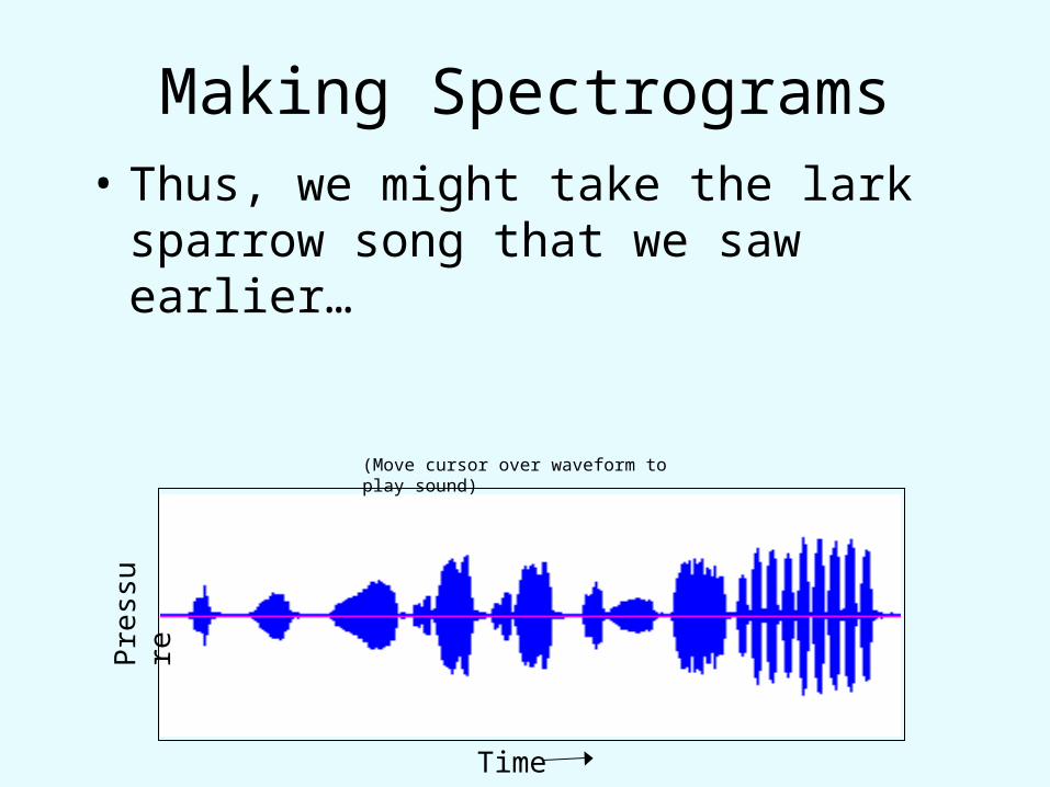
Making Spectrograms• Thus, we might take the lark sparrow song
that we saw earlier…
Pre
ssur
e
Time
(Move cursor over waveform to play sound)
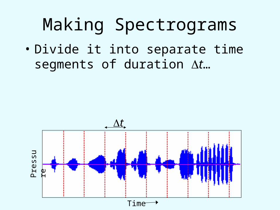
Making Spectrograms• Divide it into separate time segments of
duration t…
t
Pre
ssur
e
Time
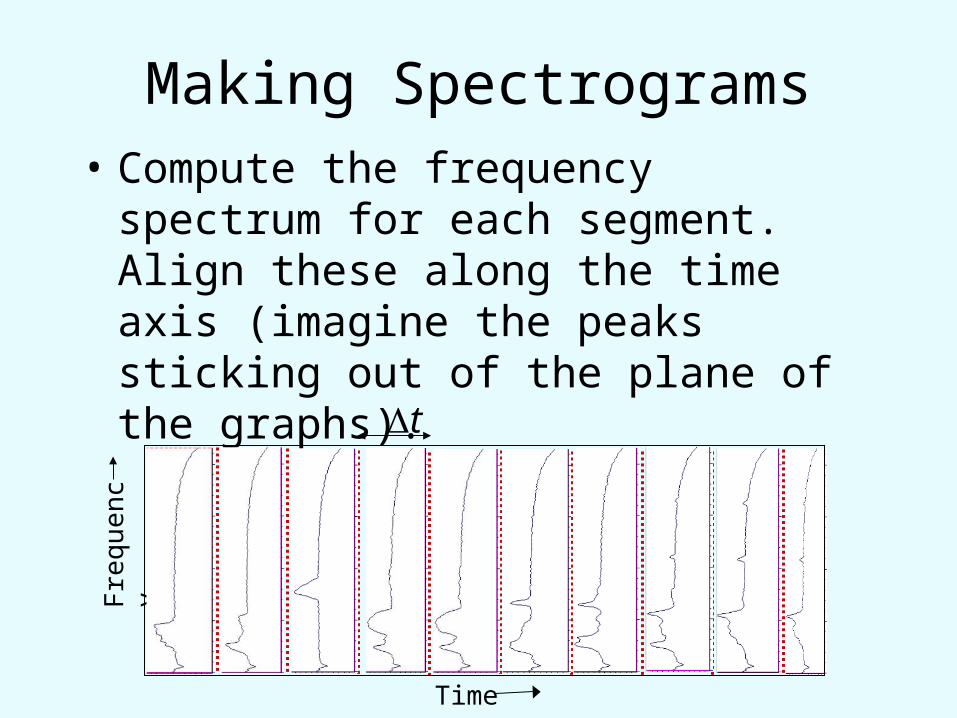
Making Spectrograms• Compute the frequency spectrum for each
segment. Align these along the time axis (imagine the peaks sticking out of the plane of the graphs).
t
Fre
quen
cy
Time
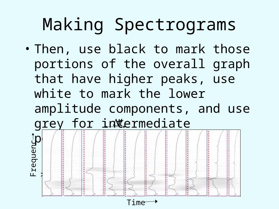
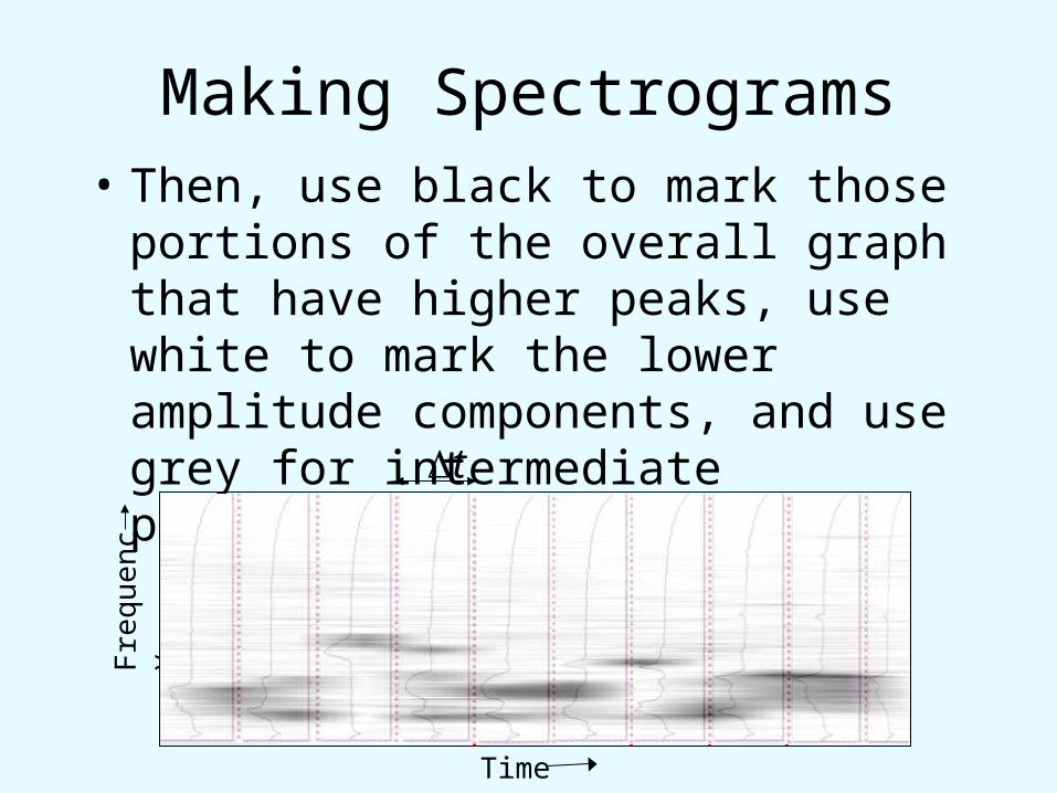
Making Spectrograms• Then, use black to mark those portions of
the overall graph that have higher peaks, use white to mark the lower amplitude components, and use grey for intermediate portions.
t
Fre
quen
cy
Time
Making Spectrograms• Then, use black to mark those portions of
the overall graph that have higher peaks, use white to mark the lower amplitude components, and use grey for intermediate portions.
t
Fre
quen
cy
Time
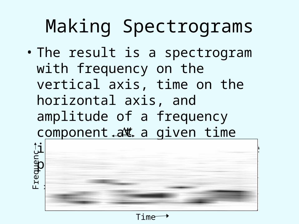
Making Spectrograms• The result is a spectrogram with frequency
on the vertical axis, time on the horizontal axis, and amplitude of a frequency component at a given time indicated by darkness on the plot.
t
Fre
quen
cy
Time
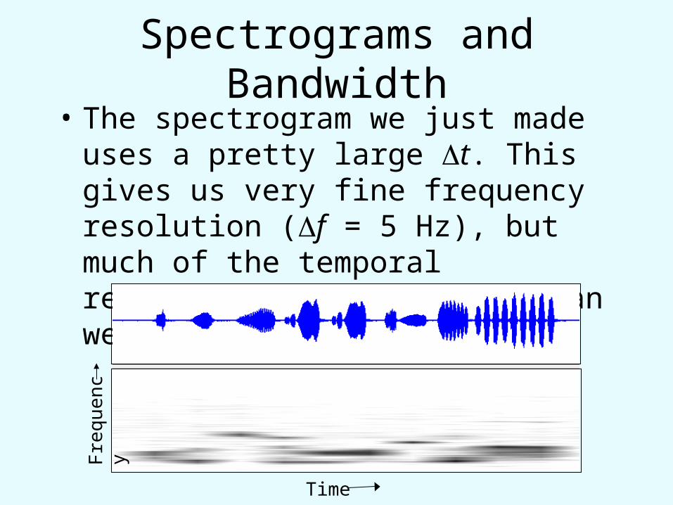
Spectrograms and Bandwidth• The spectrogram we just made uses a pretty
large t. This gives us very fine frequency resolution (f = 5 Hz), but much of the temporal resolution has been lost. Can we get by with a smaller t?
Fre
quen
cy
Time

Spectrograms and Bandwidth• Let’s decrease t by 4×. This will give us a
f = 20 Hz). This starts to restore some of the temporal pattern, and the frequency bands are still pretty thin.
Fre
quen
cy
Time

Spectrograms and Bandwidth• Let’s decrease t by 4× again. This will
give us a f = 80 Hz. We get much better temporal pattern and even some better frequency pattern because FM signals show as FM, not their components!
Fre
quen
cy
Ti×me
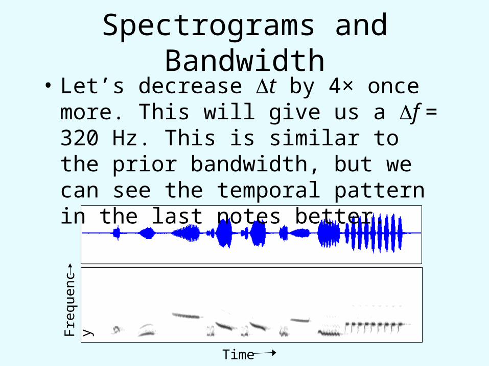
Spectrograms and Bandwidth• Let’s decrease t by 4× once more. This
will give us a f = 320 Hz. This is similar to the prior bandwidth, but we can see the temporal pattern in the last notes better.
Fre
quen
cy
Time
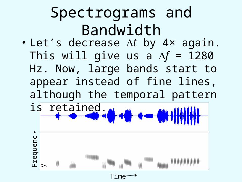
Spectrograms and Bandwidth• Let’s decrease t by 4× again. This will
give us a f = 1280 Hz. Now, large bands start to appear instead of fine lines, although the temporal pattern is retained.
Fre
quen
cy
Time
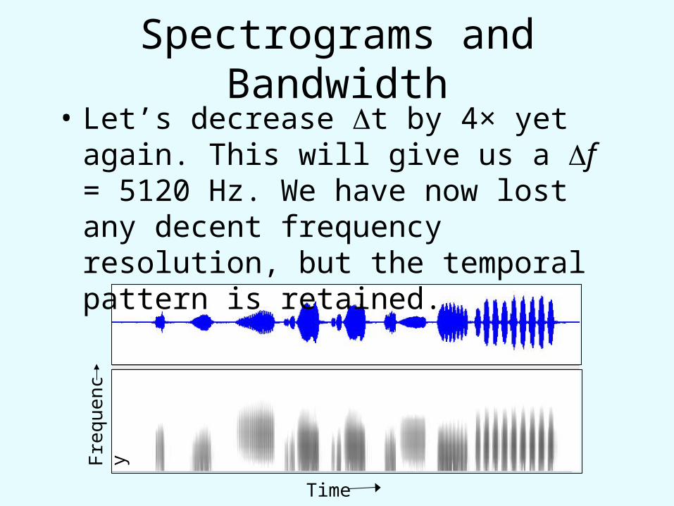
Spectrograms and Bandwidth• Let’s decrease t by 4× yet again. This will
give us a f = 5120 Hz. We have now lost any decent frequency resolution, but the temporal pattern is retained.
Fre
quen
cy
Time
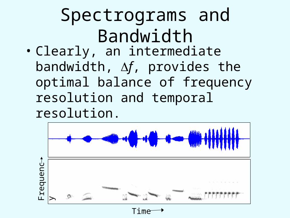
Spectrograms and Bandwidth• Clearly, an intermediate bandwidth, f,
provides the optimal balance of frequency resolution and temporal resolution.
Fre
quen
cy
Time
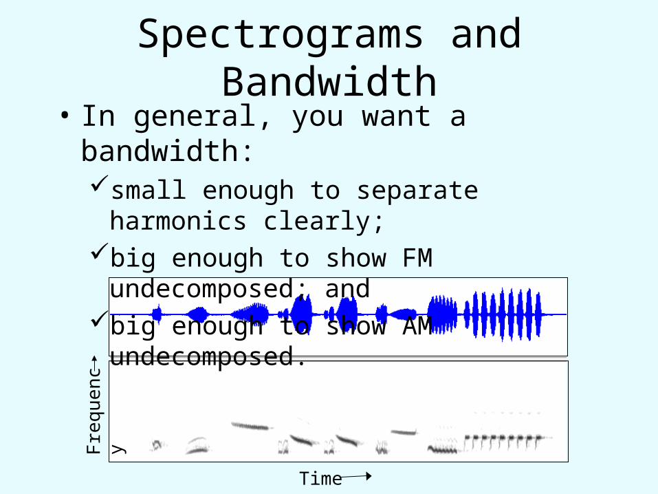
Spectrograms and Bandwidth• In general, you want a bandwidth:
small enough to separate harmonics clearly;big enough to show FM undecomposed; and big enough to show AM undecomposed.
Fre
quen
cy
Time

Digital Sound Analysis• Computers and DAT recorders sample
(digitize) the continuous rise and fall of sound amplitudes at some fixed rate and store a long column (vector) of amplitude values. Music CDs sample at 44.1 kHz.
Digital Sound Analysis• At each sample point, the computer also
digitizes the amplitude value into one of N equidistant categories. The number of categories depends on how many “bits” are used to store each value. N = 2number of bits
• Music CDs store 16 bits/sample and thus divide the full amplitude range into 216 = 65,536 possible values.
Digital Sound Analysis• The higher the sampling rate and the higher
the bit depth, the more accurately the digital recording captures the original sound.
• However, increasing sampling rate or bit depth or both increases the size of the digital file that must be stored.
• In stereo recording, two columns of numbers must be stored, taking up even more memory.

Digital Sound Analysis• Nyquist frequency: A digital recorder or
computer must be able to take at least 2 samples/cycle to be able to identify each frequency.
• Thus, if you digitize your sounds at R samples/sec, you will be unable to properly capture any component with frequency >R/2. This latter value is called the Nyquist frequency.
Digital Sound Analysis• Aliasing: If you do not sample your sounds
at a high enough rate, any frequency in the sounds that is higher than half the sampling rate is aliased. This means you will see an artifact in your spectrograms consisting of an inverted version of what the sounds should have looked like if you had sampled at a sufficiently high rate. Not nice!
Digital Sound Analysis• Digital Bandwidths: In most computer
sound analysis programs, you do not set the bandwidth f directly, but instead set the segment duration, t.
• Instead of setting a time, you indicate t by specifying the number of consecutive sample points to be used for each frequency spectrum in the spectrogram. This is often called “frame size.”
Digital Sound Analysis• Windowing: If you cut a sound directly
into segments (a rectangular window) to make a spectrogram, you introduce artifacts at the beginning and end of each segment.
• This occurs because, with rectangular windows, each segment begins with no sound and is suddenly switched “on” and suddenly “off.” The frequency spectrum of sudden onsets and offsets must contain a wide smear of frequencies.

Digital Sound Analysis• Windowing: To reduce artifacts, most
analyzers use “tapered” cutting windows (Hann, Blackman, etc.) that turn the segment off and on slowly.
Lark Sparrow
f = 320 Hz
Rectangular window
Lark Sparrow
f = 320 Hz
Blackman window