HEC MONTRÉAL

Mortgage and Mortgage-Backed Securities Valuation

par

Yann Foucault

Sciences de la gestion (Option Ingénierie financière)

Mémoire présenté en vue de l’obtention du grade de maîtrise ès sciences en gestion

(M. Sc.)

Mai 2019 © Yann Foucault, 2019

iii

Abstract

Mortgage Backed-Securities are exposed to prepayment risk, both from prepayment and

default occurring in the underlying pool of mortgages. The probability of such events is

modelled using intensity functions: prepayment is mostly driven by the current level of

interest rates relative to the mortgage contractual rate; default is primarily driven by the

ratio of the mortgage outstanding balance relative to the housing value. Interest rates are

assumed to follow an Ornstein-Uhlenbeck process, as in Vasicek. Housing prices are

modeled using a geometric Brownian motion, correlated with the interest rate process. In

order to capture a wide range of possible states for the interest rate and housing price

variables over the long life of a mortgage, a Markov chain is used, based on two grids,

one for the interest rates and one for the housing prices. To ensure housing prices do not

fall outside the bounds of the grid in spite of the housing price long-term upward drift,

only the stochastic part of the housing price dynamics gets deployed on the grid. A

mortgage is then valued using dynamic programming. The drift part of the housing price

process is calculated off-line and added at each time step to the diffusion part. The state

variable dynamics parameters are estimated using maximum likelihood. We fit the

prepayment intensity functions parameters to the observed prepayment rates by

minimizing squared differences. The model has been stress-tested and turns out to be

robust even in extreme scenarios such as negative interest rates.

Keywords : Mortgage, MBS, valuation, prepayment, default, Vasicek, geometric

Brownian motion, interest rates, housing prices, Markov chain.

iv

Table of contents

Abstract…………………………………………………………………………………iii

Table of contents………………………………………………………………………..iv

List of tables and figures………………………………………………………………..v

Acknowledgement………………………………………………………………………vi

Mortgage and Mortgage-Backed Securities Valuation………………………………….1

References……………………………………………………………………………...27

Appendices….………………………………………………………………………….28

v

List of Tables and Figures

Table 1: Housing log-return and interest-rate process parameter estimates

Figure 1: Historical spread between 15-year mortgage rate and LIBOR 1-Month (1991-

2017)

Figure 2: Model Prepayment Rate vs Historical CPR time series (FN 890404 Pool

example)

Figure 3: Impact of increasing απ on discount and premium mortgage values.

Figure 4: Student's t-test to assess reasonableness of housing and interest-rate parameter

estimates

Figure 5: Simulated Housing and Interest Rate Parameter Mean Squared Standard

Deviation vs. Sample Variance

Figure 6: Simulated Housing Parameter Estimates

Figure 7: Simulated Interest Rate Parameter Estimates

Figure 8: Simulated Correlation Parameter Estimates

Figure 9: Baseline parameters stress-testing

Figure 10: Prepayment parameters stress-testing

Figure 11: Prepayment parameters stress-testing (continued)

Figure 12: Default parameters stress-testing

Figure 13: Recovery, Ornstein-Uhlenbeck and Housing log-return process parameters

stress-testing

vi

Acknowledgement

I would like to thank my thesis advisor, Geneviève Gauthier, who patiently led me through

the process of building a model, from simpler to more complex, and taught me how to go

from the core mathematical equations to the code implementation, rather than the other

way around.

I am also very grateful to the PwC partnership, who trusted me and allowed me to

transition from an accounting to a quantitative finance role, while I was completing this

master’s diploma. A special thanks to Louis Alain, my former coach and now mentor, and

to Allen Ho, our financial risk management team partner.

Finally, I must express my profound gratitude to Phi Yen, for supporting and encouraging

a lifelong learner, who may be a bit too passionate about studying for his own good.

Mortgage and Mortgage-Backed Securities Valuation

August 4, 2019

1 Literature review

About two households out of three own their home in Canada or the US.1 A key factorbehind so high a homeownership rate lies in relatively low mortgage rates. Banks can offeraffordable rates to mortgagors, in part thanks to the existence of a secondary market. Onsuch a market, banks can quickly offload and turn into cash the mortgages they issue. Mort-gages are split, aggregated and packaged into tradeable securities, called mortgage-backedsecurities (“MBS”). Investors purchasing MBS need accurate risk-sensitive models to pricewhat they buy.

In practice, valuation models available to investors are either very simplified, using adeterministic one-size-fit-all linear prepayment model;2 or highly complex and linked to theswaption market,3 which may or may not be relevant to investors who do not use swaptionsto hedge their exposure to mortgage prepayment.

It may be useful to explore alternative valuation models that faithfully reflect the randomnature of interest rates, housing prices, prepayment and default events; incorporate stableestimates of the parameters governing the probability distribution thereof; and remain rela-tively simple numerically.

Extensive literature has been dedicated to valuing MBS. An early focus has been on therisk of early termination. At first, the emphasis was on the risk of prepayment. A singlestate variable, the interest rate, was considered (for example in Schwartz and Torous (1989)or Stanton (1995)). Then, the risk of default was also incorporated, and a second state

1For Canada, see Statistics Canada, at https://www150.statcan.gc.ca/n1/pub/11-402-x/2011000/chap/fam/fam-eng.htm. For the US, see U.S. Census Bureau, Homeownership Rate forthe United States [RHORUSQ156N], retrieved from FRED, Federal Reserve Bank of St. Louis;https://fred.stlouisfed.org/series/RHORUSQ156N, June 2, 2019.

2For a description of the PSA Prepayment Model developed by the Public Securities Association for the USin 1985 and still widely in use, see https://en.wikipedia.org/wiki/PSA prepayment model. For a Canadianequivalent tailored to National Housing Act (“NHA”) MBS, see a description of the Linear LiquidationModel at https://iiac.ca/wp-content/uploads/IIAC-MBS-Committee-NHA-MBS-Linear-Liquidation-Model-v-1.1.pdf.

3For a description of the LIBOR Market Model, used for example by Bloomberg in their MBS valuationfunctions, see Brigo and Mercurio (2007).

1

variable, the house price, was introduced (see Schwartz and Torous (1992) or Stanton et al.(2005)).

In such papers, the interest rate is modeled using a Cox-Ingersoll-Ross mean-revertingsquare-root process, and, where applicable, housing prices are assumed to follow a geometricBrownian motion correlated with the interest-rate Brownian.

For the prepayment or default function, reduced-form models have been developed, as inSchwartz and Torous (1992): mortgagors are assumed to be rational and to exercise theirprepayment or default option when it is optimal. Thus, they prepay their mortgage whencurrent rates fall below their mortgage contractual rate; and they default on their mortgagewhen the mortgaged house value falls below the value of the mortgage liability. The risk ofprepayment is captured by a hazard function whereby the prepayment intensity is a directfunction of the gap between the mortgage contract rate and the current mortgage marketrate. Similarly, the risk of default is captured by a hazard function whereby the defaultintensity is direct function of a mortgage outstanding balance to the value of the mortgagedhouse. In reduced-form models, prepayment and default function parameters are providedexogenously based on empirical observations (Schwartz and Torous (1992)).

Conversely, structural models have been developed by for example Stanton (1995). Stan-ton notes that the mortgagors’ default is not necessarily rational, as they do not exercisetheir prepayment or default option optimally. Friction or transaction costs are modeled andaim at capturing different, and suboptimal, observed behaviors among different mortgagors.Other stylized facts, such as seasoning patterns, are emphasized and modeled (Stanton).

Various numerical approaches have been implemented, from solving a partial differen-tial equation (or a couple of partial differential equations) to Monte Carlo simulations (asdescribed in Hull (2012)) to combining a binomial tree with a Monte Carlo simulation (asdescribed in Veronesi (2010)).

More recently, alternative interest rate models have been applied to valuing MBS, espe-cially the LIBOR-market model (LLM). The MBS is modeled as a tradable callable bond,the prepayment option of which could be hedged using swaptions, and the aim is to capturethe volatility skew observed on the swaption market. See for example Karpishan et al. (2010)or chapter 31 in Hull (2012).

We used a two-state-variable (interest rate and housing price) model. The interest rateand the housing prices respectively follow a single-factor Ornstein-Uhlenbeck process, as inVasicek (1977), and a Geometric Brownian motion correlated therewith. We modeled therisk of prepayment and default using two intensity functions, which express the rational be-havior of option holders, however combined with background prepayment and default rates,which translate non-rational observed behaviour. Also, as we adopt the perspective of aMBS pool on the US Agency TBA market for 15-year mortgages, where pools are fungible,mortgagor-specific transaction costs can be ignored, as the individual differences can rea-sonably be assumed to average out from the law of larger numbers. The burnout effect is

2

naturally expressed by the fact that the aggregate principal of the pool is reduced by earlierprepayments, so that the absolute prepayment amount at the pool level decreases as timepasses. The burnout effect may also be indirectly expressed by the lower intensity in thedefault function as the mortgage balance decreases (see equation (27)), so that prepaymentis cross-expressed by both the prepayment and the default function.

We implemented the valuation using dynamic programming and a two-dimensional grid,similar to the Markov-chain approach applied by Duan and Simonato (2001) to the valuationof American equity options.

We estimated the parameters in the interest-rate and housing price dynamics using log-likelihood and we estimated the parameters in the prepayment function using a least squareddifference approach.

2 Mortgage and Mortgage-Backed Securities (MBS)

Valuation Methodology

2.1 No prepayment

2.1.1 One mortgage

The monthly payment p of a mortgage with a face value F , a maturity of T months, and amonthly interest rate (coupon) C satisfies:

F = pT∑t=1

(1

1 + C

)t.

But∑T

t=1

(1

(1+C)

)t= 1

1+C

∑Tt=1

(1

1+C

)t−1, where we recognize a geometric series. Hence,

F = p1

1 + C

1−(

11+C

)T1− 1

1+C

= p1−

(1

1+C

)TC

. (1)

Therefore, the monthly payment is

p = FC

1−(

11+C

)T . (2)

Lemma 1. At month t, the balance is

Bt = F (1 + C)t(

1− (1 + C)T − (1 + C)T−t

(1 + C)T − 1

). (3)

Proof. Initially, B0 = F . Then, ∀t ∈ 1, T, the balance at t, noted Bt, equals the balanceat t− 1, less the payment made at t, net of the interest amount accrued over one period onthe t− 1-balance. In equation:

Bt = Bt−1 − (p− CBt−1) (4)

3

= Bt−1(1 + C)− p.

Using recursion over time yields

Bt = F (1 + C)t − pt−1∑u=0

(1 + C)u

= F (1 + C)t +FC

1−(

11+C

)T 1− (1 + C)t

C

= F (1 + C)t(

1− (1 + C)T − (1 + C)T−t

(1 + C)T − 1

).

2.1.2 Pool of mortgages

Exact calculations Consider a pool of M mortgages. Assume they are all issued at thesame issuance date, which matches the pool origination date, and share the same maturitydate. The initial face value is

F =M∑m=1

F (m).

The equations for the face value as a function of C, the total fixed payment, and the unpaidbalances at any time t are simple sums of the right-hand terms in equations (1), (2) and (3)respectively. Thus,

F =M∑m=1

p(m)1−

(1

1+C(m)

)TC(m)

(5)

P =M∑m=1

p(m) =M∑m=1

F (m) C(m)

1−(

11+C(m)

)T (6)

Bt =M∑m

B(m)t =

M∑m=1

F (m)(1 + C(m))t(

1− (1 + C(m))T − (1 + C(m))T−t

(1 + C(m))T − 1

). (7)

In practice, for Fannie Mae Single-Family MBS, coupon information available to investorsused to be limited to the pool average coupon, and some percentiles. Since January 1, 2013,individual loan-level information has been available.4 On the to-be-announced (TBA) market,such information is however pointless, as MBS security holders do not know which pool, froma cohort of thousands, will be assigned to their security. Hence the need to work with cohortaverages.

4See Fannie Mae PoolTalk c© FAQ’s, retrieved from http:www.fanniemae.com/resources/file/mbs/pdf/mbsfaqs.pdfon April 26, 2018.

4

Average-based calculations Define the original-balance-weighted average of the mort-gage coupons:

C =M∑m=1

F (m)

FC(m). (8)

Then, similar to equation (1), P , an approximation to the pool aggregate fixed payment,satisfies

F = PT∑t=1

(1

1 + C

)t.

Therefore,

P = FC

1−(

11+C

)T . (9)

As a corollary, similar to equation (3),

Bt = F (1 + C)t(

1− (1 + C)T − (1 + C)T−t

(1 + C)T − 1

). (10)

Remark The total monthly payment P , from equation (6) is different from a fixed monthlypayment calculated at the pool level using C and a maturity of T ≥ maxm(T (m)), as is donein equation (9):

P =FC

1−(

11+C

)T =

∑Mm=1 F

(m)C(m)

1−(

1

1+∑Mm′=1

F (m′)F

C(m′)

)T .In the case where all coupon rates C(m) and all maturities T (m) are the same, then C(m) = C,T (m) = T and

P =M∑m=1

F (m)C

1−(

1

1+C∑Mm′=1

F (m′)F

)T =M∑m=1

F (m)C

1−(

11+C

)T = P.

Likewise, Bt 6= Bt.Nevertheless, C, P , and Bt are reasonable approximations for C, P , and Bt when projectingthe cash flows of a pool underlying an MBS, since pooled mortgages share similar terms andcoupons.

2.1.3 Mortgage-backed security (MBS)

Principal payments are passed through integrally to MBS holders. F and Bt, as defined for apool in equations (5) and (7), or the approximation of the latter, Bt, as described in equation(10), also apply to the related MBS.Interest payments are passed through at a reduced rate C < C, net of servicing fees (paid tothe mortgage servicer) and a credit risk compensation (paid to the guarantor Agency). Based

5

on C as defined in equation (8), a reasonable projection for the MBS payment in month t isthen, from equation (4):

Pt = Bt−1(1 + C)− Bt

= Bt−1(1 + C − C + C)− Bt

= Bt−1(1 + C)− Bt − Bt−1(C − C)

= P − Bt−1(C − C).

Conclusion A bank who lends money to mortgagors will show them the coupon C, thepayment p and the resulting mortgage balance amortizing schedule made up of Bt. Suchnumbers may be “customer-friendly”, but they are not the whole story. Where does thiscoupon C come from?

2.2 Prepayment

Consider again a single mortgage.

2.2.1 Mortgage valuation

A mortgage is exposed to interest rate risk, default risk, and prepayment risk throughout itslife.

Risk-free rate The risk-free rate rt satisfies

drt = α (β − rt) dt+ σdW P,rt , (11)

where

• β is the interest rate long-term average;

• α is the speed of mean-reversion;

• W P,r is a Brownian motion under the physical probability measure P.

Housing price The housing price satisfies

dHt = µH,tHtdt+ σHHtdWP,Ht , (12)

where

• Ht is the housing price at time t, which can be proxied by some housing index;

• µH is the housing price log-return drift;

• σH is the housing price log-return volatility.

6

Moreover,

Corr(W P,rt ,W P,H

t

)= ρ ∀t > 0.

Therefore, we can write W P,H = ρW P,rt +

√1− ρ2W P,⊥

t , where W P,r and W P,⊥ are two inde-pendent Brownian motions. The state variables rt and Ht generate a filtration F, to whichis associated a σ-algebra (Ft)t≥0.

Risk-neutral world In a risk-neutral world,

WQ,rt = W P,r

t +

∫ T

0

γrsds

and

WQ,Ht = W P,H

t +

∫ T

0

γHs ds.

If the Novikov condition is satisfied, there is a probability measure Q equivalent to P suchthat

•dQdP

= exp

(−∫ T

0

γrsdWP,rs −

∫ T

0

γ⊥s dWP,⊥s − 1

2

∫ T

0

(γrs)2 + (γ⊥s )2ds

)• WQ,r and WQ,⊥ are two independent Q-Brownian motions.

Now, with respect to the Brownian associated with housing prices,

γHt =µH − rtσH

. (13)

Replacing rt with its definition (see equation (30) in section 3.1.1 further down), and usingJensen inequality and Fubini’s theorem,5 it would be possible to show that

EP[exp

(1

2

∫ T

0

(γHs ds

)2)]

<∞, (14)

so that the Novikov condition is satisfied.

Default time In continuous time, let Λ(η)t be the default intensity at time t. The default

time is

τη = inft > 0 :

∫ t

0

Λ(η)s ds > E1

where E1 is an exponential random variable of expectation 1 independent of W P,r and W P,⊥.In that case, the conditional survival probability with respect to default is

P(τη > T

Gt) = EP[exp

(−∫ T

t

Λ(η)s ds

)Gt] δτη>t, (15)

where5See for example https://math.stackexchange.com/questions/133691/can-i-apply-the-girsanov-theorem-

to-an-ornstein-uhlenbeck-process.

7

• δ is an indicator function;

• Gt = Ft ∨ H(η)t ∨ H

(π)t , with G = F ∨ H(η) ∨ H(π). H(η)

t is a σ-algebra associated with

the filtration H(η) generated by the indicator of default. H(π)t is a σ-algebra associated

with the filtration H(π) generated by the indicator of prepayment (see below). Ft is aσ-algebra associated with F, the filtration generated by the state variables rt and Ht

as already defined. The objective probability measure P is thus defined on the filteredprobability space Ω,P,G,Gt≥0.

Prepayment time Similarly, let Λ(π)t be the prepayment intensity at time t. The prepay-

ment time is

τπ = inft > 0 :

∫ t

0

Λ(π)s ds > E2,

where E2 is an exponential random variable of expectation 1 independent of W P,r, W P,⊥, andE1.The conditional survival probability with respect to prepayment

P(τπ > T

Gt) = EP[exp

(−∫ T

t

Λ(π)s ds

)Gt] δτπ>t.(16)

Risk-free discount factor Let the risk-free discount factor be

D(RF )t,T = exp

(−∫ T

t

rs ds

)Mortgage value Let t∗i = i∆t, with ∆t set to one month. A mortgage at time t∗i is worth

Vt∗i = EQ

[N∑

j=i+1

D(RF )t∗i ,t∗j

pδτη>t∗j δτπ>t∗j︸ ︷︷ ︸regular payment

+κBt∗j−1δt∗j−1<τη≤t∗j δτπ>t∗j︸ ︷︷ ︸

payment on default

+Bt∗j−1(1 + C)δt∗j−1<τπ≤t∗j δτη>t∗j︸ ︷︷ ︸

prepayment

Gt∗i

δτη>t∗i δτπ>t∗i ,(17)

where N is the total number of monthly payments stipulated in the mortgage agreement, κis the recovery rate, comprised between 0 and 1, in the event of a default, and i is a timeindex for such payments.6

6Equation (17) makes implicitly two assumptions. First, it assigns a probability of nil to the case whendefault and prepayment occur simultaneously, as both events can reasonably be considered mutually exclusive.Second, it assumes that a mortgage can only be prepaid in full, never in part. Arguably, curtailments havea much milder financial impact that full prepayment to a lender and can reasonably be ignored. Moreover,our model could still handle partial prepayments: it would suffice to subdivide a given mortgage into smallerbalances and apply equation (17) to such balances separately.

8

Using the tower property of conditional expectations and recursion,

Vt∗i = EQ[D

(RF )t∗i ,t∗i+1

pδτη>t∗i+1

δτπ>t∗i+1+ κBt∗i

δt∗i<τη≤t∗i+1δτπ>t∗i+1

+Bt∗i(1 + C)δt∗i<τπ≤t∗i+1

δτη>t∗i

Gt∗i ] δτη>t∗i δτπ>t∗i+ EQ

[D

(RF )t∗i ,t∗i+1

EQ

[N∑

j=i+2

D(RF )t∗i+1,t

∗j

pδτη>t∗j δτπ>t∗j + κBt∗j−1

δt∗j−1<τη≤t∗j δτπ>t∗j

+Bt∗j−1(1 + C)δt∗j−1<τπ≤t∗j δτη>t∗j

Gt∗i+1

]δτη>t∗i+1

δτπ>t∗i+1

Gt∗i ] δτη>t∗i δτπ>t∗i= EQ

[D

(RF )t∗i ,t∗i+1

pδτη>t∗i+1

δτπ>t∗i+1+ κBt∗i

δt∗i<τη≤t∗i+1δτπ>t∗i+1

+Bt∗i(1 + C)δt∗i<τπ≤t∗i+1

δτη>t∗i

Gt∗i ] δτη>t∗i δτπ>t∗i+ EQ

[D

(RF )t∗i ,t∗i+1Vt∗i+1

Gt∗i ] δτη>t∗i δτπ>t∗i= EQ

[D

(RF )t∗i ,t∗i+1

(p+ Vt∗i+1

)δτη>t∗i+1

δτπ>t∗i+1+ κBt∗i

δt∗i<τη≤t∗i+1δτπ>t∗i+1

+Bt∗i(1 + C)δt∗i<τπ≤t∗i+1

δτη>t∗i

Gt∗i ] δτη>t∗i δτπ>t∗i .

(18)

Further,

dQdP

Ft∗i+1

dQdP

Ft∗i

D(RF )t∗i ,t∗i+1

= exp

(−∫ t∗i+1

t∗i

γrsdWP,rs −

∫ t∗i+1

t∗i

γ⊥s dWP,⊥s − 1

2

∫ t∗i+1

t∗i

(γr)2 + (γ⊥)2ds−∫ t∗i+1

t∗i

rsds

) (19)

Time discretization Let ti =t∗i∆t

, so that ti = i for i ∈ 0, T∆t. In discrete time, equations

(11) and (21) respectively become

rti+1= rti + α (β − rti) ∆t + σ

(W P,rt∗i+1−W P,r

t∗i

)(20)

andHti+1

= Hti + µHHti∆t + σHHti

(W P,Ht∗i+1−W P,r

t∗i

). (21)

Then,

D(RF )ti,ti+1

= exp

(−∫ t∗i+1

t∗i

rs ds

)' 1

exp (rti∆t)' 1

1 + rti∆t

.

9

Similarly, discretizing equation (19) yields

dQdP

Fti+1

dQdP

Fti

D(RF )ti,ti+1

' 1

1 + γrti

W P,rt∗i+1−W P,r

t∗i︸ ︷︷ ︸'0

+ γ⊥ti

W P,⊥t∗i+1−W P,⊥

t∗i︸ ︷︷ ︸'0

+ rti∆t + 12

(γrti)

2 + (γ⊥ti )2

∆t

' 1

1 + rti∆t +1

2

(γrti)

2 + (γ⊥ti )2

∆t︸ ︷︷ ︸spread

.

Assume γr and γ⊥ are constant. We are left with the following risky discount factor underP:

Dti,ti+1=

1

1 + rti∆t + 12(γr)2 + (γ⊥)2∆t

=1

1 + (rti + S) ∆t

(22)

where S is a constant risky spread.

Also, going back to the prepayment probabilities in equation (18), from discretizing equa-tions (15) and (16) respectively, we get

EP[δτη≥t∗i+1

Gt∗i ] = P(τη > t∗i+1

Gt∗i ) ' EP[exp

(−Λ

(η)t∗i

∆t

)Gt∗i ] δτη>t∗i (23)

andEP[δτπ≥t∗i+1

Gt∗i ] = P(τπ > t∗i+1

Gt∗i ) ' EP[exp

(−Λ

(π)t∗i

∆t

)Gt∗i ] δτπ>t∗i . (24)

As a result, in a discrete time version of equation (18), a mortgage at time i∆t is worth

Vi∆t = EP[D(i∆t,(i+1)∆t)

(p+ V(i+1)∆t

)exp

(−Λ

(η)i∆t

∆t

)exp

(−Λ

(π)i∆t

∆t

)+κBi∆t

(1− exp

(−Λ

(η)i∆t

∆t

))exp

(−Λ

(π)i∆t

∆t

)+Bi∆t(1 + C)

(1− exp

(−Λ

(π)i∆t

∆t

))exp

(−Λ

(η)i∆t

∆t

)Gi∆t

]δτη>i∆tδτπ>i∆t .

(25)

Relationship between prepayment and default Recall that prepayment and defaultare assumed to be mutually exclusive. The mortgage termination time is the minimum be-tween two stopping times, τη and τπ, and is thus itself a stopping time. Default is mostlydriven by the gap between the mortgage unpaid balance and the house value: the greater thegap, the greater the probability of default, as US mortgagors may walk away from both theirhouse and mortgage, thus getting rid of a liability which is larger than their asset. Prepay-ment is mostly driven by the gap between the mortgage coupon C and current mortgage rate

10

Ct, which makes currently issued mortgages trade at par. We can therefore model defaultand prepayment as two separate functions.

Such a model handles the cases when mortgagors may both want to default and prepay.This is reflected in positive probabilities for both default and prepayment. The relativemagnitude of the default intensity rate, a function of the ratio mortgage unpaid balance tohouse price, versus the prepayment intensity rate, a function of the difference between themortgage coupon and the current mortgage rate,7 will automatically make default probabilitygreater than prepayment probability.8

2.2.2 Determining the fair coupon at inception

In equation (25), p, C, and Bt are given to the investors, and Vti does not need to equal F .But to a mortgage issuer, at ti = 0, i.e. on the issuance date, the fair coupon needs to bedetermined by setting V0 equal to F and solving for p (or C). Then, using equations (2) and(3), C (or p) and Bs,∀ s ∈ 1, T, can be found.

2.3 Default intensity function

Temporarily ignore the possibility of prepayment, and focus on default.

Recall equation (21). Housing price log-returns are modelled as following a geometricBrownian motion:

Hti+1= Hti exp

((µH,t −

σ2H

2

)∆t+ σH

(W

(P,H)t∗i+1

−W (P,H)t∗i

)). (26)

The higher the ratio of Bti — the mortgage yet unpaid balance when mortgagors may debatewhether to default at time ti+1 — to the house value Hti , the higher the mortgagors debt

relative to the backing asset, and the more likely a default. A time t0, set Ht0 =Bt0υ

, where υis the average loan-to-value ratio at origination, as observed on the market at the time of themortgage issuance.9 The one-period default intensity in equation (23) can thus be specifiedas

Λ(η)ti = aη + bη

(min

[Bti

Hti

, 1

])cη, (27)

where

• aη+bη is a positive constant background default rate, to be estimated. Its interpretationis that a default may occur for other reasons than a high unpaid balance relative to thehouse value. Such events are captured by aη;

7For details about such functions, see sections 2.3 and 2.4 further below.8This is different from Schwartz and Torous (1992), who model the interaction between default and

prepayment using two functions by part, both conditioned on housing prices and mortgage rates, and set theprobability of default (prepayment) to zero when prepayment (default) dominates default (prepayment). SeeSection 1 for more details.

9Such a ratio typically hovers around 0.8.

11

• bη, a positive constant, may have a magnifying or reducing effect, whether it is smalleror greater than 1;

• cη is a positive constant ≥ 1, since Λη is expected to be increasing and convex inBti−1

Hti;

• the minimum function ensures the default rate accelerates as cη increases.

• The interpretation of the floor set to 1 is that, when the mortgage balance is smallerthan the house value, the mortgagor has no economic incentive to default. The onlysource of default is then the constant background rate aη + bη, described further above.

Remark Going back to equation (23), observe how, the greater the ratio of Bti to Hti ,

the greater Λ(η)ti , and so the smaller the survival probability exp

(−Λ

(η)ti

)and the greater the

default rate 1− exp(−Λ

(η)ti

)and the probability of defaulting at ti+1.

2.4 Prepayment intensity function

Ignore temporarily the possibility of default. At any time tj,10 mortgagors may compare the

holding value of their mortgage, noted V(h)ti , and the prepayment or exercise value V

(e)ti . They

want to minimize their liability, so that, the wider the gap between V(h)ti and V

(e)ti , the greater

the incentive to prepay.

The prepayment intensity in equation (24) is defined as

Λ(π)ti =

(aπ + bπ

([V

(h)ti − V

(e)ti

]+)cπ)

, (28)

with aπ, bπ, and cπ, respectively similar to aη, bη, and cη as already defined in equation (27).Taking the positive part of the expression ensures that the intensity remains positive.

If the mortgagors hold to their mortgage, they owe p, the payment scheduled for tj, plusthe present value of their current mortgage remaining payments, that is Vtj+1

, from equation(17), multiplied by the one-month discounting factor Dtj ,tj+1

. If they refinance, they onlyowe CBtj−1

,11 the interest owing for the period just ended in tj, plus the expected present

value of a new mortgage, V(Ctj )

tj , the coupon of which, Ctj , makes said present value equal to

par, i.e. Btj−1, which is the opening balance for period tj.

12 We thus have that

V(h)tj = EP [Vtj+1

Gtj]Dtj ,tj+1+ p,

V(e)tj = Btj−1

(1 + C) ,

10We assume here that default or prepayment can occur at the end of a period only.11Recall that no prepayment penalty applies to mortgages underlying Fannie Mae conventional MBS.12In equation (25), Btj−1 is substituted to Vtj on the left-hand side, and the currently observed mortgage

rate Ctj , as well as a corresponding fixed payment ptj are substituted to C and p, while every remainingfuture balance Btj−1

in the sum gets updated accordingly, so that the equality is satisfied.

12

so that, equation (28) becomes

Λ(π)tj = aπ + bπ

([EP [Vtj+1

Gtj]Dtj ,tj+1+ p−Btj−1

(1 + C)]+)cπ

, (29)

where Vtj+1is obtained from equation (25).13

3 Numerical implementation

3.1 State variable dynamics and probability calculations

Such a valuation model can be implemented using a time sequence of two-dimensional grids,with one axis for the housing price diffusion term and the other axis for the interest ratediffusion term. The information from both housing prices and interest rates feeds into thedefault and prepayment functions, as defined by equations (23) and (24). Using a Markovchain, and moving backwards through such a sequence of grids from the mortgage matu-rity date to the valuation date, we can thus calculate the default probability, the prepaymentprobability and the continuation probability at each node. The value of the mortgage at eachnode is the probability-weighted average of such three values, as described in more detail inequations (36) further below. Moving back from time step to time step to the valuation dateultimately yields the mortgage present value, weighted by the different path probabilities,and discounted accordingly.

3.1.1 The interest rate dynamics

The solution to the Ornstein-Uhlenbeck equation (11) is

rt = β + e−αt (r0 − β) + σ

∫ t

0

e−α(t−s)dW (Q)s (30)

Writing the Ornstein-Uhlenbeck process as an autoregressive process of order 1, or AR(1),yields

rtj+1= e−α∆trtj + β

(1− e−α∆t

)+ σ

√1− e−2α∆t

2αZtj+1

, (31)

where Ztjj∈N are i.i.d standard normal random variables, and ∆t = 112

.

Define the diffusion term

xtj+1= σ

√1− e−2α∆t

2αZtj+1

= rtj+1−(e−α∆trtj + β

(1− e−α∆t

)),

which will become handy in calculating transition probabilities further down.

13For a detailed description of the recursive implementation of the mortgage valuation, moving backwardsfrom Vtj+1 to EP [Vtj+1

Gtj ] and Vtj , see Section 3.

13

We now build a grid for interest rate values. We center the grid around β, the distributionlong-term reverting mean. We set r(N), the upper bound of the grid, to the maximum levelobserved in US short-term interest rate empirical time series over the last 30 years, i.e. 10%,which was reached by LIBOR 1-month in March 1989. We then observe that a 33 basis pointrate decrease would save a typical $150,000-indebted Fannie Mae 15-year mortgagor $500 inannual interest payments, a difference that could trigger prepayment. So we determine thatphysical increments should be no more than 33 basis points, and we set such increments,noted ∆x, to 0.33% / 5. This yields a grid of equally spaced interest rates r(n), ranging from10% to β − (10%− β).14

Finally, ∀n ∈ 2, N − 1, we partition the vector into cells (Dn, Dn+1], with Dn =r(n−1)+r(n)

2, so that every interest rate level r(n) is the midpoint in a vector cell. Further,

set D1 = −∞ and DN+1 =∞.

3.1.2 The housing price dynamics

Turning to housing price dynamics, discretizing equation (26) gives

Htj+1= Htj exp

((µH,tj −

σ2H

2

)∆t + σH

√∆t Z

(H)tj+1

)(32)

where µH,tj = µH − γHσH = rt, with µH as defined in equation (26) and γH as defined inequation (13).

A challenge is to build a grid that is wide enough to cover every reasonable state of Htj

over up to 15 years, subject to computer memory constraints.15 A solution, suggested byDuan and Simonato [5] for equity prices S, is to define an adjusted asset price St rid of thedrift term such that

Stj = Stj exp(−µ(S)j∆t

)= S0 exp

(σS√j∆t

J∑j=1

Z(S)tj

), (33)

where S0 is the asset price at the asset valuation date and µ(S) is the drift parameter for S.

We cannot exactly replicate such a scheme since, in equation (32), the drift term µ(P,H)tj

is not a constant, but a stochastic rt. We can however build, in the same spirit, a grid forthe housing dynamic diffusion part.16

Let M , the number of elements in the housing price vector, be any odd positive integer,only subject to computer memory constraints. We build the grid of housing prices in two

14N , the number of grid points is thus a function of β. We estimate β to be 0.0174 in section 4.1. As aresult, N equals 250.

15Using MATLAB on a Windows Intel i5-7003U system at 2.60 GHz with 16 GB memory, we couldimplement, with a monthly discretization, a 250-by-180 node interest rate grid and a 49-by-180 node housingprice grid.

16Denoted ht, as defined further down in section 3.1.3.

14

steps: first, a temporary grid, where H0 coincides with a grid node; second, the final grid isobtained from slightly shifting the temporary grid, so that H0 falls exactly in the middle ofthe grid middle node.

Let’s label the temporary grid nodes C. And let the middle node C(M+12

) = H0. Fur-

ther, set the grid upper and lower bounds to C(M+12

) +√

M−12σH√

∆t

√tJ and C(M+1

2) −√

M−12σH√

∆t

√tJ respectively, where tJ = T , the mortgage fixed maturity date.17 Subdi-

vide the intervall thus bounded into M − 1 subintervalls of equal size18

∆C ≈ 2

√M−1

2σH√

∆t

√tJ

M − 1.

Then, ∀m ∈ 2,M−1, partition the vector into cells (C(m), C(m+1)], with C(m) = C(m−1)+C(m)

2,

so that, in particular, H0 = C(M2 )+C(M2 +1)

2as planned. Further, set C(1) = −∞ and C(M+1) =

∞.

Remark Rather than simply centering the housing diffusion term tree around H0, it wouldmake sense to center such a tree around H0 plus β, the interest rate long-term averageparameter, or a weighted average of such variables. However, a grid simply centered aroundH0 performs adequately, including in very high or very low interest rate environments, asevidenced in our stress test.19

3.1.3 The bivariate transition probabilities

Let p(mn,uv) be, ∀m,∀u ∈ 1,M and ∀n,∀v ∈ 1, N, the joint transition probability underthe probability measure P that both

• the housing reference price move from state H(m), at any time tj, to state H(u) at timetj+1, and

• the interest rate move from state r(n), at any time tj, to state r(v) at time tj+1.

17Setting M = 101, for example, thus yields upper and lower bounds 7.91σ apart from the middle nodesince T is fixed and equal to 15 years, regardless of the remaining term-to-maturity at the valuation date.

18See Duan and Simonato [5] for such a choice of ∆h, which helps ensure convergence.19See section 5 for stress-tests.

15

In equation,

p(mn,uv) = P(Cu < Htj+1

≤ Cu+1 andDv < rtj+1≤ Dv+1

Htj = H(m) and rtj = r(n))

= P(Cu < Htj exp

((µH,tj −

σ2

2

)∆t + σH

√∆tZtj+1

)≤ Cu+1

andDv < rtj+1≤ Dv+1

Htj = H(m) and rtj = r(n))

= P(

ln

(CuH(m)

)<

(µH,tj −

σ2

2

)∆t + σH

√∆tZtj+1

≤ ln

(Cu+1

H(m)

)andDv −

(e−α∆tr(n) + β

(1− e−α∆t

))< rtj+1

−(e−α∆tr(n) + β

(1− e−α∆t

))≤ Dv+1 −

(e−α∆tr(n) + β

(1− e−α∆t

)) Htj = H(m) and rtj = r(n))

= P(

ln

(CuH(m)

)−(r(n) + γHσH −

σ2

2

)∆t < σH

√∆tZtj+1

≤ ln

(Cu+1

H(m)

)−(r(n) + γHσH −

σ2

2

)∆t

andDv −(e−α∆tr(n) + β

(1− e−α∆t

))< rtj+1

−(e−α∆tr(n) + β

(1− e−α∆t

))≤ Dv+1 −

(e−α∆tr(n) + β

(1− e−α∆t

)) Htj = H(m) and rtj = r(n)).

(34)

Define

c(m)u = ln

(CuH(m)

)−(r(n) + γHσH −

σ2

2

)∆t

andd(n)v = Dv −

(e−α∆tr(n) + β

(1− e−α∆t

)).

Also define the housing price dynamics diffusion term

htj+1= σH

√∆t Z

(H)tj+1

= σH√

∆t

(ρZtj+1

+√

1− ρ2Z(⊥)tj+1

)with Corr

(Ztj+1

, Z(⊥)tj+1

)= 0, and Z(⊥)

tj j∈N i.i.d.N(0, 1).

16

Then, substituting c(m)u , d

(n)v , htj+1

and xtj+1into equation (34) yields

p(mn,uv) = P(d(n)v < xtj+1

≤ d(n)v+1 and c(m)

u < htj+1≤ c

(m)u+1

)= P

d(n)v

σ√

1−e−2α∆t

2α

< Ztj+1≤

d(n)v+1

σ√

1−e−2α∆t

2α

andc

(m)u

σH√

∆t

< ρZtj+1+√

1− ρ2Z(⊥)tj+1≤

c(m)u+1

σH√

∆t

)

=

∫ d(n)v+1

σ

√1−e−2α∆t

2α

d(n)v

σ

√1−e−2α∆t

2α

∫ c

(m)u+1

σH√

∆t−ρz

√1−ρ2

c(m)u

σH√

∆t−ρz

√1−ρ2

φ(z(⊥))dz(⊥)

φ(z)dz

=

∫ d(n)v+1

σ

√1−e−2α∆t

2α

d(n)v

σ

√1−e−2α∆t

2α

Φ

c(m)u+1

σH√

∆t− ρz√

1− ρ2

− Φ

c(m)u

σH√

∆t− ρz√

1− ρ2

φ(z)dz,

(35)

where φ and Φ are respectively probability density and cumulative distribution functions ofa standard normal random variable. We implement such a double integral using MATLABmvncdf function.

3.2 Mortgage valuation using dynamic programming

First, default intensity values and one-step discount factors can be calculated off-line.

For all m ∈ 1,M, for all j ∈ 1, J, and for any n ∈ 1, N, the (mn)-node default

intensity Λ(η)(m)tj can be calculated using equation (27). H

(m)tj in the equation can be recovered

from the stationary grid at each time step by combining H(m), β and tj as follows:20

H(m)tj ≈ H0 exp

((β − σ2

2

)j∆t +

((m− M + 1

2

)∆h

)).

For all n ∈ 1, N, for all j ∈ 1, J, and for any m ∈ 1,M, the (mn)-node discount

factor D(n)ti,ti+1

= 11+(r(n)+S)∆t

, from equation (22).

Then the backward algorithm can be run, starting from the maturity date.

Consider V(mn)tJ−1

, the mortgage value at time J − 1 on node (mn), where HtJ−1= H(m)

20The long term average parameter for the interest rate dynamic is used as a reasonable approximation torecover the housing prices from the stochastic interest rate rt.

17

and rtJ−1= r(n). Using equation (25) with i = J − 1 yields

VtJ−1= EP

[DtJ−1,tJ

(p+ VtJ ) exp

(−Λ

(η)tJ−1

∆t

)exp

(−Λ

(π)tJ−1

∆t

)+κBtJ−1

(1− exp

(−Λ

(η)tJ−1

∆t

))exp

(−Λ

(π)tJ−1

∆t

)+BtJ−1

(1 + C)(

1− exp(−Λ

(π)tJ−1

∆t

))exp

(−Λ

(η)tJ−1

∆t

)GtJ−1

]δτη>tiδτπ>ti .

(36)

At maturity time tJ , there is no future payment left, so VtJ = 0. Also, immediately aftertJ−1, prepayment becomes irrelevant, so that

EP[exp

(−Λ

(π)tJ−1

∆t

)]= 1.

Moreover, knowing the mortgage is still alive at tJ−1, δτη>tJ−1= 1 and δτπ>tJ−1

= 1. Equation(36) thus simplifies to

V(mn)tJ−1

= D(n)tJ−1,tJ

[p exp

(−Λ

(η)(m)tJ−1

∆t

)+ κBtJ−1

(1− exp

(−Λ

(η)(m)tJ−1

∆t

))].

Set V(uv)tJ−1

= V(mn)tJ−1

, and move one time step back, to tJ−2, where, for any of the M times Npairs (mn),

V(mn)tJ−2

= EP [DtJ−2,J−1

pδτη>tJ−1

δτπ>tJ−1+ κBtJ−2

δtJ−2<τη≤tJ−1δτπ>tJ−1

+BtJ−2(1 + C)δtJ−2<τπ≤tJ−1

δτη>tJ−1+ VtJ−1

δτη>tJ−1δτπ>tJ−1

GtJ−2

]δτη>tJ−2

δτπ>tJ−2

= D(n)tJ−2,J−1

[exp

(−Λ

(η)(m)tJ−2

∆t

)exp

(−Λ

(π)(n)tJ−2

∆t

)(p+

M∑u=1

N∑v=1

p(mn,uv)V(uv)tJ−1

)+ κBtJ−2

(1− exp

(−Λ

(η)(m)tJ−2

∆t

))exp

(−Λ

(π)(n)tJ−2

∆t

)+BtJ−2

(1 + C)(

1− exp(−Λ(π)(n)tJ−2

∆t

)exp

(−Λ

(η)(m)tJ−2

∆t

)],

(37)

where Λ(π)(n)tJ−2

is the prepayment intensity Λ(π)tJ−2

, as defined by equation (29), associated with

interest rate r(n) and continuation value∑M

u=1

∑Nv=1 p(mn,uv)V

(uv)tJ−1

. From equation (29), ∀j ∈1, J,

Λ(π)tj

(n) = aπ + bπ

(max

[EP [Vtj+1

Gtj]D(n)tj ,tj+1

+ p−Btj−1(1 + C), 0

])cπ= aπ + bπ

(max

[M∑u=1

N∑v=1

p(mn,uv)V(uv)tj+1

D(n)tj ,tj+1

+ p−Btj−1(1 + C), 0

])cπ

.

Moving further backwards until time ti yields the mortgage value Vti , as in equation (25), asat the valuation date.

18

4 Parameter estimation

4.1 Housing Price and Interest Rate Dynamics Parameter Esti-mation

Recall that a time step ∆t is equal to one month. Let k = tk, the index for such time steps,and define hk = ln(Hk). Recall the discretization for the interest dynamics from equation(31) and apply a similar discretization to equation (26) with respect to the housing pricelog-returns. We thus have

hk = hk−1 +

(µH,k−1 −

σ2H

2

)∆t + σH

√∆t Z

(H)k

and

rk = e−α∆trk−1 + β(1− e−α∆t

)+ σ

√1− e−2α∆t

2αZk

where Z(H)k k∈N and Zkk∈N are i.i.d standard normal random variable, with

Corr(Z(H)k , Zk) = ρ.

Let Σ be the variance-covariance matrix for hk and rk. Denote Σ−1 its inverse, andΣ,

its determinant. We then have

Σ =

σ2H∆t ρσH

√∆t σ

√1−e−2α∆t

2α

ρσH√

∆t σ√

1−e−2α∆t

2ασ2(

1−e−2α∆t

2α

) ,

Σ =

(1− ρ2

)σ2H∆t σ

2

(1− e−2α∆t

2α

),

and

Σ−1 =1Σ σ2

(1−e−2α∆t

2α

)−ρσH

√∆t σ

√1−e−2α∆t

2α

−ρσH√

∆t σ√

1−e−2α∆t

2ασ2H∆t

=

1

(1−ρ2)σ2H∆t

−ρ√

2α

(1−ρ2)σH√

∆t σ√

1−e−2α∆t

−ρ√

2α

(1−ρ2)σH√

∆t σ√

1−e−2α∆t

2α

(1−ρ2)σ2(1−e−2α∆t)

.

19

The joint probability density function at time k∆t

f(hk, rk)

=1√

2πΣ exp−1

2

[hk − hk−1 − (rk−1 + γHσH)∆t +

σ2H2 ∆t

rk − e−α∆trk−1 − β(1− e−α∆t

) ]′Σ−1

[hk − hk−1 − (rk−1 + γHσH)∆t +

σ2H2 ∆t

rk − e−α∆trk−1 − β(1− e−α∆t

) ]

=1√

2πΣ exp−1

2

1

(1− ρ2)σ2H∆t

(hk − hk−1 − (rk−1 + γHσH)∆t +

σ2H

2∆t

)2

− 2ρ√

2α

(1− ρ2)σH√

∆t σ√

1− e−2α∆t

(hk − hk−1 − (rk−1 + γHσH)∆t +

σ2H

2∆t

)(rk − e−α∆trk−1 − β

(1− e−α∆t

))+

2α

(1− ρ2)σ2 (1− e−2α∆t)

(rk − e−α∆trk−1 − β

(1− e−α∆t

))2.

The log-likelihood function

L(γH , σH , α, β, σ, ρ) = ln

(N∏k=1

(f(hk, rk

hk−1, rk−1

))=

N∑k=1

(ln(f(hk, rk

hk−1, rk−1

))= −N ln

(√2π)−N ln

(√1− ρ2σH

√∆t σ

√1− e−2α∆t

2α

)

− 1

2

N∑k=1

1

(1− ρ2)σ2H∆t

(hk − hk−1 − (rk−1 + γHσH)∆t +

σ2H

2∆t

)2

− 2ρ√

2α

(1− ρ2)σH√

∆t σ√

1− e−2α∆t

(hk − hk−1 − (rk−1 + γHσH)∆t +

σ2H

2∆t

)(rk − e−α∆trk−1 − β

(1− e−α∆t

))+

2α

(1− ρ2)σ2 (1− e−2α∆t)

(rk − e−α∆trk−1 − β

(1− e−α∆t

))2.

Maximizing the expression above is equivalent to minimizing its negative, without the con-stant term N ln

(√2π), that is

g(γH , σH , α, β, σ, ρ) = N ln

(√1− ρ2σH

√∆t σ

√1− e−2α∆t

2α

)

+N∑k=1

1

2 (1− ρ2)σ2H∆t

(hk − hk−1 − (rk−1 + γHσH)∆t +

σ2H

2∆t

)2

− ρ√

2α

(1− ρ2)σH√

∆t σ√

1− e−2α∆t(hk − hk−1 − (rk−1 + γHσH)∆t +

σ2H

2∆t

)(rk − e−α∆trk−1 − β

(1− e−α∆t

))+

α

(1− ρ2)σ2 (1− e−2α∆t)

(rk − e−α∆trk−1 − β

(1− e−α∆t

))2.

20

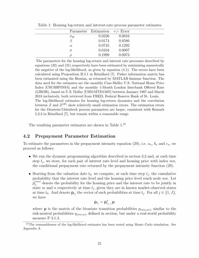
Table 1: Housing log-return and interest-rate process parameter estimates

Parameter Estimation +/- ErrorσH 0.0226 0.0016β 0.0174 0.0586α 0.0745 0.1292σ 0.0104 0.0007ρ 0.1999 0.0973

The parameters for the housing log-return and interest rate processes described byequations (32) and (31) respectively have been estimated by minimizing numericallythe negative of the log-likelihood, as given by equation (4.1). The errors have beencalculated using Proposition B.5.1 in Remillard [7]. Fisher information matrix hasbeen estimated using the Hessian, as returned by MATLAB fminunc function. Thedata used for the estimates are the monthly Case-Shiller U.S. National Home PriceIndex [CSUSHPINSA] and the monthly 1-Month London Interbank Offered Rate(LIBOR), based on U.S. Dollar [USD1MTD156N] between January 1987 and March2018 inclusively, both retrieved from FRED, Federal Reserve Bank of St. Louis.The log-likelihood estimates for housing log-return dynamics and the correlationbetween Z and Z(H) show relatively small estimation errors. The estimation errorsfor the Ornstein-Uhlenbeck process parameters are larger, consistent with Remark5.2.3 in Remillard [7], but remain within a reasonable range.

The resulting parameter estimates are shown in Table 1.21

4.2 Prepayment Parameter Estimation

To estimate the parameters in the prepayment intensity equation (29), i.e. aπ, bπ and cπ, weproceed as follows:

• We run the dynamic programming algorithm described in section 3.2 and, at each timestep tj, we store, for each pair of interest rate level and housing price with index mn,the conditional prepayment rate returned by the prepayment intensity function (29).

• Starting from the valuation date t0, we compute, at each time step tj, the cumulativeprobability that the interest rate level and the housing price level reach node mn. Letp

(mn)tj denote the probability for the housing price and the interest rate to be jointly in

state m and n respectively at time tj, given they are in known market-observed statesat time t0. And denote ptj the vector of such probabilities at time tj. For all j ∈ 1, J,we have

ptj = pᵀtj−1

p

where p is the matrix of the bivariate transition probabilities p(mn,uv), similar to therisk-neutral probabilities q(mn,uv) defined in section, but under a real-world probabilitymeasure P 3.1.3.

21The reasonableness of the log-likelihood estimates has been tested using Monte Carlo simulation. SeeAppendix A.

21

• At each time step, we compute our model monthly conditional prepayment rate, notedΨtj , as being the conditional prepayment rates returned by the prepayment intensity

function defined by equation (29) on every node mn, weighted by the probabilities p(mn)tj

to be on such nodes respectively. In equation:

Ψtj =M∑u=1

N∑v=1

pᵀp(:,uv) exp(−Λ

(uv)tj

),

where p(:,uv) is a vector column listing the transition probabilities of moving from everypair of states mn to the state uv.

• We calculate the sum of the squared differences between each element in the vector ofour model conditional probabilities Ψtj and the monthly conditional prepayment rate(“CPR”) observed on the market in the corresponding month tj.

22

• We obtain aπ, bπ and cπ estimates by minimizing such a squared difference using theMATLAB function fmincon and the interior-point algorithm.

To illustrate, consider the Fannie Mae pool with Bloomberg ticker FN 890404.23 Such apool was issued on May 1, 2012, with a 6.5% coupon. Trading above par, it is helpful in es-timating prepayment parameters, as its higher-than-market undelying coupons are expectedto trigger prepayments. Its weighted average coupon (“WAC”), or C as defined by equation(8), was 7.055% on issuance, and this is the coupon we use.

Seven years of observation are available, yielding a time series of 72 monthly conditionalprepayment rates as at April 30, 2018. Over such a period, the default rate has been nil inthe pool, based on the default rate reported by Bloomberg. This allows us to temporarilyignore the default parameters, and estimate the prepayment parameters separately.

Recall that our model stipulates, as a simplifying assumption, a constant risky spread.Observe figure 1 and note how such an assumption has held historically in the US since 1991on relatively short periods of two years or so, but should be reconsidered for longer periods.This is a limitation of our model that we acknowledge. Such an assumption is however rea-sonable for the period May 2012-April 2018, when the 15-year mortgage spread over LIBOR1-month, on a monthly basis, ranges from 174 basis points (“bps”) to 338 bps, with a 265bps average and a 43 bps standard deviation.

We first estimate the constant spread S, as defined in equation (22), by taking the differ-ence between the market average mortgage rate and the 1-month US LIBOR rates prevailingon May 1, 2012, the beginning of our estimation period.24 We estimate S to be equal to

22The market-observed CPR is obtained from Bloomberg. It is the ratio of the aggregate amount prepaidon a mortgage pool to Bt−1 − P , where B and P are as defined in equations (6) and (7), while t − 1 refersto the previous month.

23The pool CUSIP is 31410LGM8.24The mortgage rate is obtained from the Federal Reserve Bank of St. Louis. The 1-Month London Inter-

bank Offered Rate (LIBOR), based on U.S. Dollar [USD1MTD156N], from ICE Benchmark AdministrationLimited (IBA), and the US average 15-year mortgage rate were retrieved from FRED, Federal Reserve Bankof St. Louis; https://fred.stlouisfed.org/series/USD1MTD156N, June 9, 2018.

22

Figure 1: Historical spread between 15-year mortgage rate and LIBOR 1-Month (1991-2017)

2.7674%.

Then we follow the steps in the estimation procedure described further above. Minimizingthe sum of squared differences between the Ψtj values for all j ∈ 1, 72 and the 72 monthlyCPR observed on the market 25for the pool being valued yields the following estimates forfor aπ, bπ and cπ respectively: 0.000088732, 0.0011 and 1.2336.

Observe in figure 2 how the implied prepayment rates follow a much smoother trendthan the actual CPR observed for the sample pool and don’t appear to overfit. Note alsohow the model prepayment rates start high and decrease slowly from about 30% to 20%approximately, which is consistent with the historical trend, as well as the fact that muchlower interest rates than the pool coupons prevailing at the time of issuance would trigger alot of early payments.26

4.3 Default Parameters Estimation

Now that prepayment parameters have been estimated, it is possible to identify pools withnon-null default rates and estimate default parameters aη, bη and cη by minimizing thesquared difference between the monthly default rate implied by such parameters in our modeland the series of default rates observed historically.

25The CPR are obtained from Bloomberg.26Recall we are dealing with 15-year Fannie Mae MBS, which are typically backed by refinancing mortgages.

The pattern of prepayment rates starting low and increasing for two years and a half before plateauing, whichis typical of many new mortages and reflected in the well-known Public Securities Association (PSA) modelthus do not apply.

23

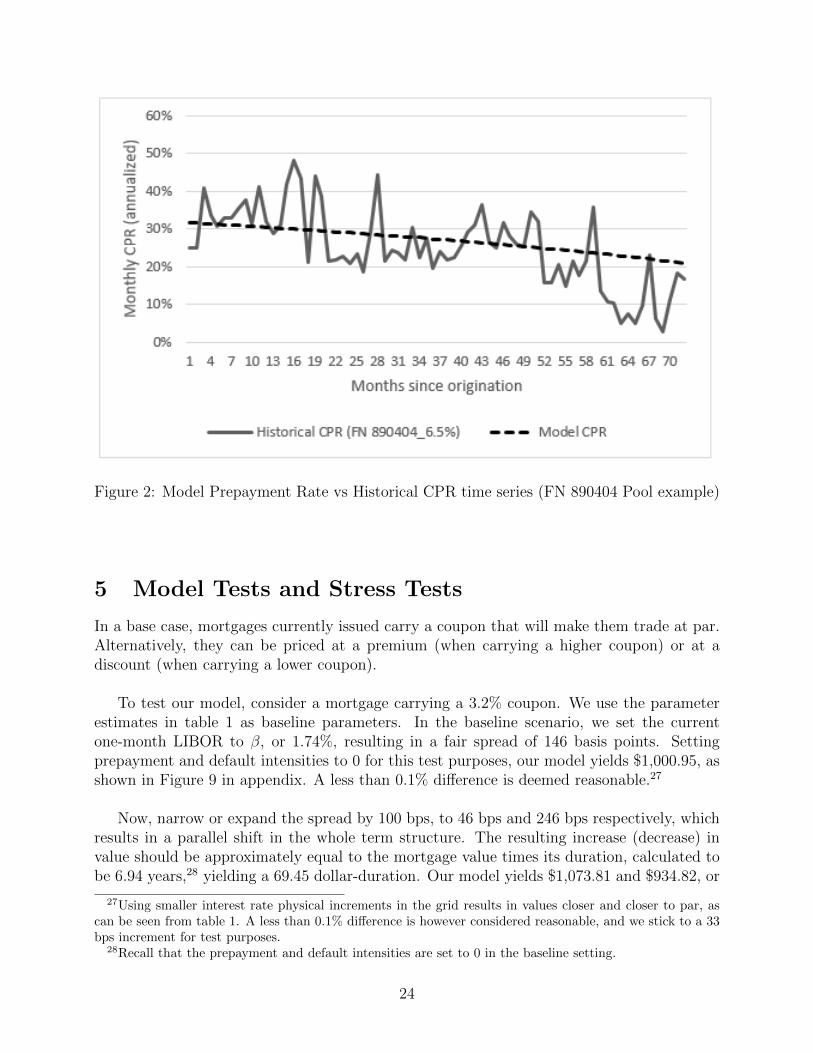
Figure 2: Model Prepayment Rate vs Historical CPR time series (FN 890404 Pool example)

5 Model Tests and Stress Tests

In a base case, mortgages currently issued carry a coupon that will make them trade at par.Alternatively, they can be priced at a premium (when carrying a higher coupon) or at adiscount (when carrying a lower coupon).

To test our model, consider a mortgage carrying a 3.2% coupon. We use the parameterestimates in table 1 as baseline parameters. In the baseline scenario, we set the currentone-month LIBOR to β, or 1.74%, resulting in a fair spread of 146 basis points. Settingprepayment and default intensities to 0 for this test purposes, our model yields $1,000.95, asshown in Figure 9 in appendix. A less than 0.1% difference is deemed reasonable.27

Now, narrow or expand the spread by 100 bps, to 46 bps and 246 bps respectively, whichresults in a parallel shift in the whole term structure. The resulting increase (decrease) invalue should be approximately equal to the mortgage value times its duration, calculated tobe 6.94 years,28 yielding a 69.45 dollar-duration. Our model yields $1,073.81 and $934.82, or

27Using smaller interest rate physical increments in the grid results in values closer and closer to par, ascan be seen from table 1. A less than 0.1% difference is however considered reasonable, and we stick to a 33bps increment for test purposes.

28Recall that the prepayment and default intensities are set to 0 in the baseline setting.

24

0.4% and 0.5% from the expected approximate values, which again is reasonable.

We stress the current interest rate to a high (low, and even negative) level and verify thatthe value make sense, falling to $711.23 (increasing to $1177.30).

If the term structure is flat, a mortgage trading at par should not be sensitive to prepay-ment. We set the prepayment background intensity parameter aπ to 1

∆tand verify than the

model yields a $1,000 value.

A mortgage trading at a premium (discount) should decrease (increase) in value as pre-payments increase and early-returned capital gets to be reinvested at a lower (higher) rate.But, assuming there is no risk of default, a mortgage value cannot fall below (rise above) par.So we set the intensity of default to zero, and vary aπ from 1

∆tto 1

1000∆tfor both a premium

and a discount mortgage. Note how aπ = 1∆t

is an extreme case, as it translates into a 63.21%monthly prepayment rate. Figure 3 shows how both mortgage values are bounded betweenpar and the no-prepayment value, and exhibit a decreasing or increasing trend to par as theprepayment rate increases (from right to left on the graph).29

Figure 3: Impact of increasing aπ on discount and premium mortgage values.

We expect the multiplying factor in Λπ, bπ as defined in equation (29) to have a similar

29For the exact values used to generate this graph, the various parameter precise settings, as well as furthercomments about the results reasonableness, please refer to the table in figure 10 in the appendix. The sameor similar tables in the appendix back all figures in this stress-testing section.

25

effect as aπ. Focusing on the premium mortgage, and setting aπ and the exponent cπ toneutral values (0 and 1 respectively), we can verify in the table labeled Figure 10 that, again,the mortgage value decreases from the no-prepayment premium value to par as bπ increases(from bottom to top in the table).

More generally, the model returns values that are consistent with our reasonable expec-tations as can be see in figures 9, 10, 11,12 and 13 in Appendix B.

26

References

[1] Damiano Brigo and Fabio Mercurio, Interest Rate Models - Theory and Practice, SecondEdition, Springer, 2007.

[2] Chris Downing, Richard Stanton and Nancy Wallace, An Empirical Test of a Two-Factor Mortgage Valuation Model: How Much Do House Prices Matter?, Real EstateEconomics, vol. 33(4), 681-710, Winter 2005.

[3] John C. Hull, Options, Futures, and Other Derivatives, 8th ed., Prentice Hall, 2012.

[4] John C. Hull and Alan D. White, Numerical Procedures for Implementing Term Struc-ture I, The Journal of Derivatives Fall 1994, 2 (1) 7-16.

[5] Jin-Chuan Duan and Jean-Guy Simonato, American Option Pricing under GARCH by aMarkov Chain Approximation, Journal of Economic Dynamics Control, 25, 1689-1718,2001.

[6] Yakov Karpishan, Ozgur Turel and Alexander Hasha, Introducing the Citi LMM TermStructure Model for Mortgages, The Journal of Fixed Income, 20, 1, 44-58, Summer2010.

[7] Bruno Remillard, Statistical Methods for Financial Engineering, CRC Press, 2013.

[8] Eduardo S. Schwartz and Walter N. Torous, Prepayment and the Valuation of Mortgage-Backed Securities, The Journal of Finance, vol. XLIV, NO.2, 375-392, June 1989.

[9] Eduardo S. Schwartz and Walter N. Torous, Prepayment, Default, and the Valuation ofMortgage Pass-Through Securities, The Journal of Business, vol. 64, issue 2, 221-239,April 1992.

[10] Richard Stanton, Rational Prepayment and the Valuation of Mortgage-Backed Securi-ties, Review of Financial Studies, 8, 677-708, 1995.

[11] Oldrich Vasicek, An equilibrium characterization of the term structure, Journal of Fi-nancial Economics (1977) vol. 5, issue 2, 177-188.

[12] Pietro Veronesi, Fixed Income Securities: Valuation, Risk, and Risk Management, JohnWiley & Sons, 2010.

27

Appendix A. Verifying the reasonableness of the housing

and interest rate process parameter estimates

We verify whether the estimates presented in section 4.1 are reasonable and our log-likelihoodformula implementation is accurate as follows:

• Using the parameters in table 1, we simulate 100 paths of monthly housing index valuesand interest rates over five years of housing prices and interest rates (resulting in 100bivariate series of 60 time points);

• We estimate the sample parameters using the log-likelihood function and minimizationapproach described above;

• We compare the parameter sample means to the theoretical parameters and test thehypothesis that they are similar using a Student’s t-test.

• We compare the sample variance for each parameter to the corresponding mean squaredstandard deviation, i.e.

S2θ

=1

n

n∑i=1

S2θi

(38)

where Sθi is the standard deviation of any given parameter θ (i.e either µH ,30 σH , β,α, σ, or ρ) across the 100 simulations performed.

As can be seen in Figure 4, the estimates appear to be reasonable at a 95% confidencelevel, except for µH and α. With respect to µH however, the sample mean is arguably rea-sonably close to the theoretical value, being 3.45% compared to 3.68%. With respect to α,the test negative result is consistent with the large estimation error noted in Table 1. Furtherwork could be devoted to explore how to better estimate Vasicek dynamic parameters. Thisis beyond the scope of this Master’s thesis.

As shown in Figure 5, S2 looks reasonably close to the sample variance for every param-eter, again except for α.

One can also verify visually in Figures 6, 7 and 8 that, except for alpha, for reasons alreadyexplained, the parameter estimates resulting from the 100 simulations performed reasonablybracket the theoretical value.

30For the purpose of this test, we used a constant housing drift parameter. Further work could be devotedto estimating the risk premium.

28

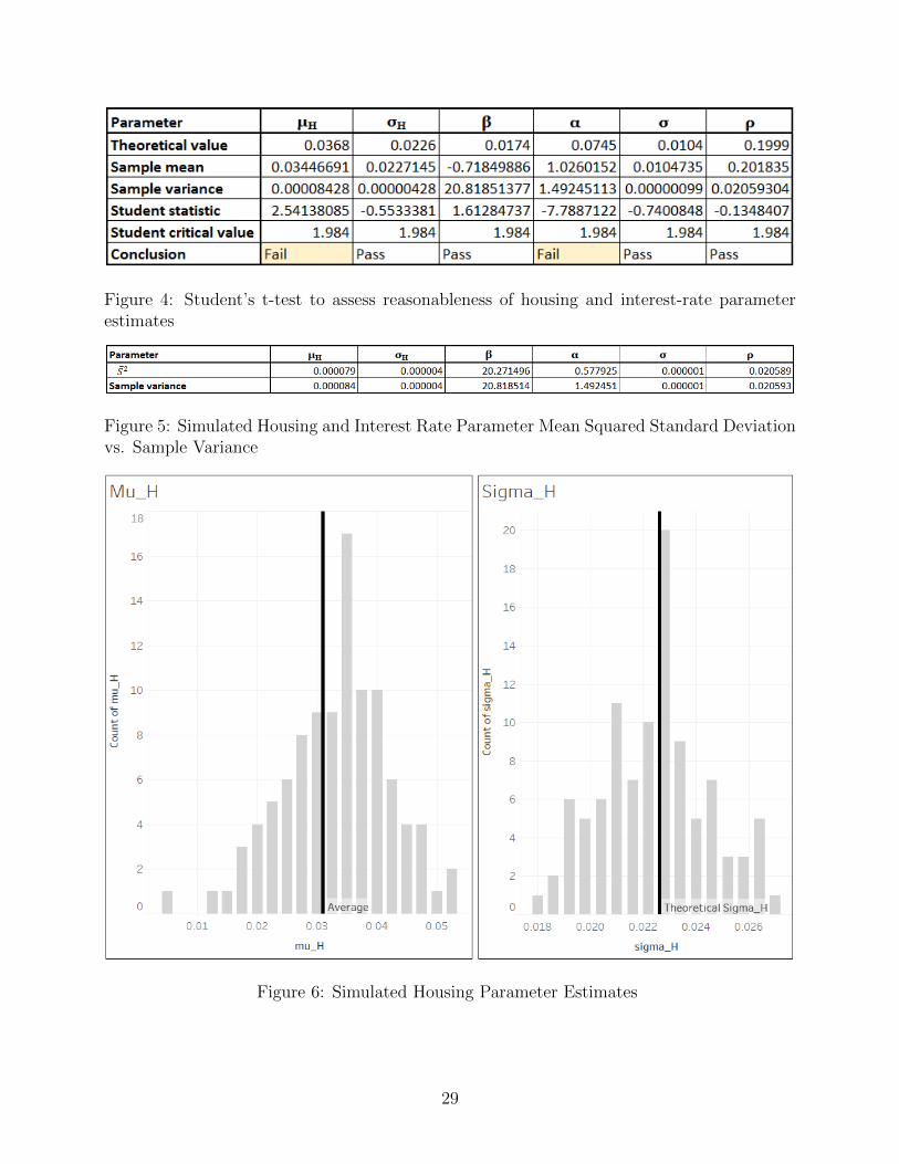
Figure 4: Student’s t-test to assess reasonableness of housing and interest-rate parameterestimates

Figure 5: Simulated Housing and Interest Rate Parameter Mean Squared Standard Deviationvs. Sample Variance

Figure 6: Simulated Housing Parameter Estimates

29

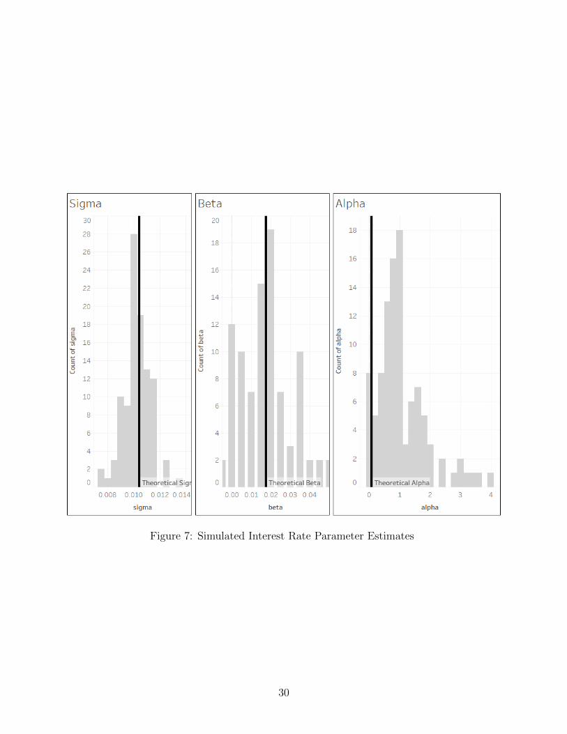
Figure 7: Simulated Interest Rate Parameter Estimates

30

Figure 8: Simulated Correlation Parameter Estimates

31

Appendix B. Stress Tests

32

Fig

ure

9:B

asel

ine

par

amet

ers

stre

ss-t

esti

ng

33

Fig

ure

10:

Pre

pay

men

tpar

amet

ers

stre

ss-t

esti

ng

34

Fig

ure

11:

Pre

pay

men

tpar

amet

ers

stre

ss-t

esti

ng

(con

tinued

)

35

Fig

ure

12:

Def

ault

par

amet

ers

stre

ss-t

esti

ng

36

Fig

ure

13:

Rec

over

y,O

rnst

ein-U

hle

nb

eck

and

Hou

sing

log-

retu

rnpro

cess

par

amet

ers

stre

ss-t

esti

ng

37