Preferences, Utility, Budget Line and Consumer Equilibriumirfanlal.yolasite.com/resources/Consumer...
58
Preferences, Utility, Budget Line and Consumer Equilibrium Consumer Theory
-
Upload
hoangkhuong -
Category
Documents
-
view
227 -
download
3
Transcript of Preferences, Utility, Budget Line and Consumer Equilibriumirfanlal.yolasite.com/resources/Consumer...

Preferences, Utility, Budget
Line and Consumer
Equilibrium
Consumer Theory
The Household’s Budget
Consumption Possibilities
A household’s consumption possibilities are constrained
by its income and the prices of the goods and services it
buys.
A household has a given amount of income to spend and
cannot influence the prices of the goods and services it
buys.
A household’s budget line describes the limits to a
household’s consumption choices.
The Household’s Budget
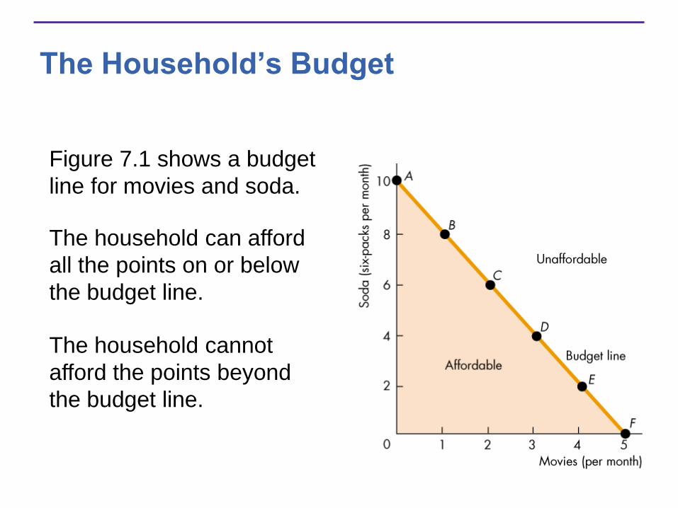
Figure 7.1 shows a budget
line for movies and soda.
The household can afford
all the points on or below
the budget line.
The household cannot
afford the points beyond
the budget line.
The Household’s Budget
Relative Price
A relative price is the price of one good divided by the
price of another good.
The price of a movie is $6 and the price of soda is $3 a
six-pack.
So the relative price of a movie is $6 per movie divided by
$3 per six-pack, which equals 2 six-packs per movie.

The Household’s Budget
A Price Change
A change in the price of
the good on the x-axis
changes the affordable
quantity of that good and
changes the slope of the
budget line.
Figure 7.2(a) shows the
rotation of a budget line
after a change in the
relative price of movies.
The Household’s Budget
Real Income
A household’s real income is the household’s income
expressed as the quantity of goods that the household can
afford to buy.
Expressed in terms of soda, Lisa’s real income is 10 six-
packs—the maximum quantity of six-packs that she can
buy.
Lisa’s real income equals her money income ($30) divided
by the price of a six-pack ($3).
The Household’s Budget
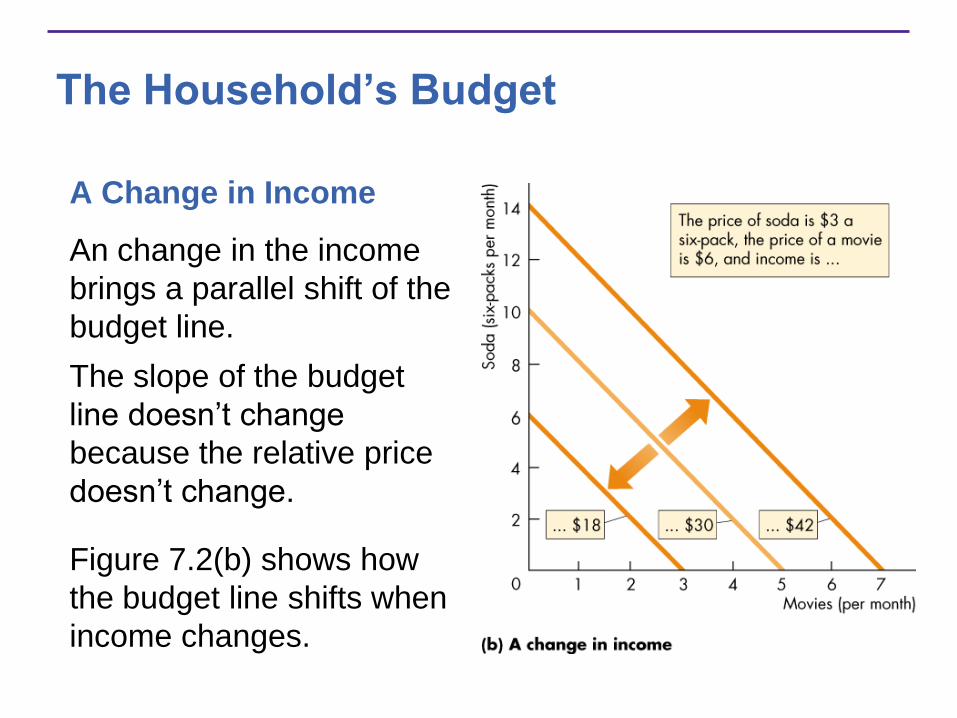
A Change in Income
An change in the income
brings a parallel shift of the
budget line.
The slope of the budget
line doesn’t change
because the relative price
doesn’t change.
Figure 7.2(b) shows how
the budget line shifts when
income changes.
Preferences and Utility
Preferences
A household’s preferences determine the benefits or
satisfaction a person receives consuming a good or
service.
The benefit or satisfaction from consuming a good or
service is called utility.
Total Utility
Total utility is the total benefit a person gets from the
consumption of goods. Generally, more consumption
gives more utility.
Preferences and Utility
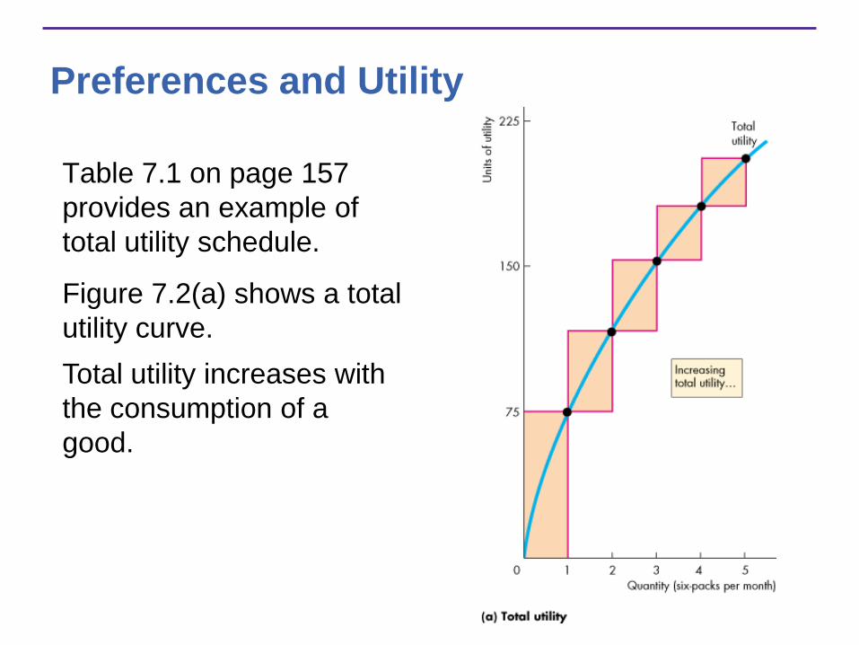
Table 7.1 on page 157
provides an example of
total utility schedule.
Figure 7.2(a) shows a total
utility curve.
Total utility increases with
the consumption of a
good.

Preferences and Utility
Marginal Utility
Marginal utility is the change in total utility that results
from a one-unit increase in the quantity of a good
consumed.
As the quantity consumed of a good increases, the
marginal utility from consuming it decreases.
We call this decrease in marginal utility as the quantity of
the good consumed increases the principle of diminishing
marginal utility.
Preferences and Utility
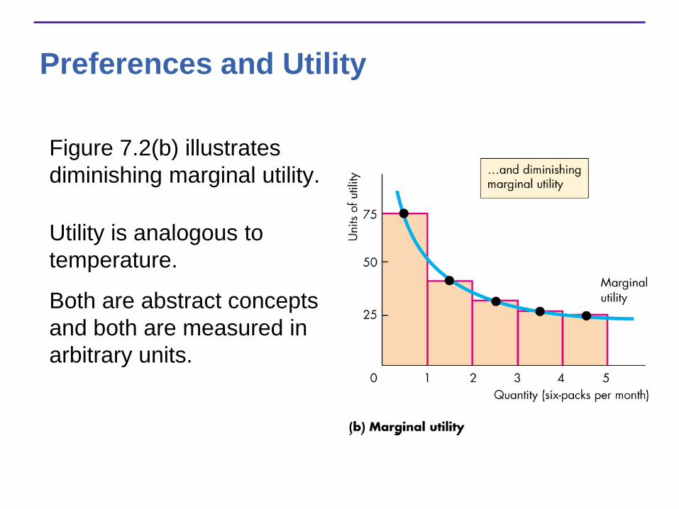
Figure 7.2(b) illustrates
diminishing marginal utility.
Utility is analogous to
temperature.
Both are abstract concepts
and both are measured in
arbitrary units.

Maximizing Utility
The key assumption of marginal utility theory is that the
household chooses the consumption possibility that
maximizes total utility.
The Utility-Maximizing Choice
We can find the utility-maximizing choice by looking at the
total utility that arises from each affordable combination.
Table 7.2 (page 158) shows an example of the utility-
maximizing combination, which is called a consumer
equilibrium.

Maximizing Utility
Equalizing Marginal Utility per Dollar
Using marginal analysis, a consumer’s total utility is
maximized by following the rule:
Spend all available income and equalize the marginal
utility per dollar for all goods.
The marginal utility per dollar is the marginal utility from
a good divided by its price.

Maximizing Utility
The Utility-Maximizing Rule:
Call the marginal utility of movies MUM .
Call the marginal utility of soda MUS .
Call the price of movies PM .
Call the price of soda PS .
The marginal utility per dollar from seeing movies is
MUM/PM .
The marginal utility per dollar from soda is MUS/PS.
Maximizing Utility
Total utility is maximized when:
MUM/PM = MUS/PS
Table 7.3 (page 159) and Figure 7.4 on the next slide
show why the utility maximizing rule works.

Maximizing Utility
If MUM/PM > MUS/PS,
then moving a dollar from
soda to movies increases
the total utility from movies
by more than it decreases
the total utility from soda,
so total utility increases.
Only when MUM/PM =
MUS/PS, is it not possible
to reallocate the budget
and increase total utility.
Maximizing Utility
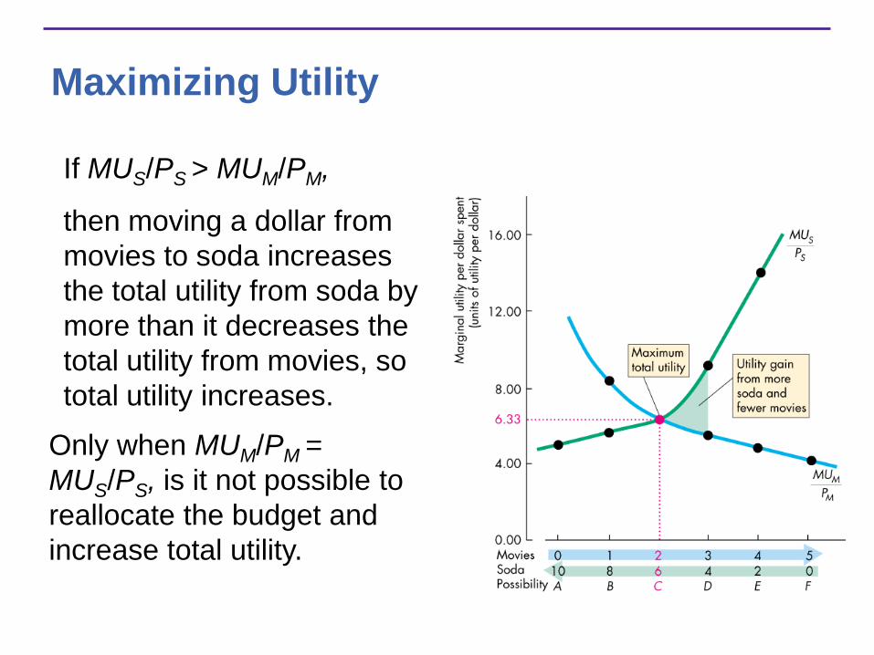
If MUS/PS > MUM/PM,
then moving a dollar from
movies to soda increases
the total utility from soda by
more than it decreases the
total utility from movies, so
total utility increases.
Only when MUM/PM =
MUS/PS, is it not possible to
reallocate the budget and
increase total utility.
Predictions of Marginal Utility Theory
A Fall in the Price of a Movie
When the price of a good falls the quantity demanded of
that good increases—the demand curve slopes
downward.
For example, if the price of a movie falls, we know that
MUM/PM rises, so before the consumer changes the
quantities consumed, MUM/PM > MUS/PS.
To restore consumer equilibrium (maximum total utility)
the consumer increases the quantity of movies consumed
to drive down the MUM and restore MUM/PM = MUS/PS.
Predictions of Marginal Utility Theory
A change in the price of one good changes the demand
for another good.
You’ve seen that if the price of a movie falls, MUM/PM
rises, so before the consumer changes the quantities
consumed, MUM/PM > MUS/PS.
To restore consumer equilibrium (maximum total utility)
the consumer decreases the quantity of soda consumed to
drive up the MUS and restore MUM/PM = MUS/PS.

Consumption Possibilities
Household consumption choices are constrained by its
income and the prices of the goods and services available.
The budget line describes the limits to the household’s
consumption choices.
Consumption Possibilities
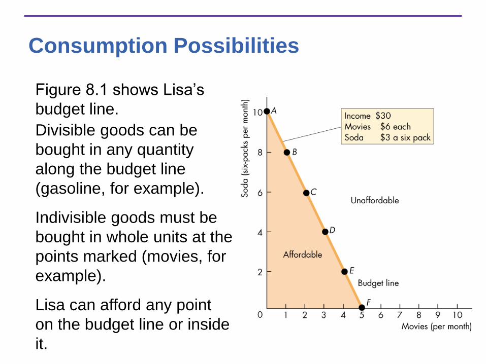
Figure 8.1 shows Lisa’s
budget line.
Divisible goods can be
bought in any quantity
along the budget line
(gasoline, for example).
Indivisible goods must be
bought in whole units at the
points marked (movies, for
example).
Lisa can afford any point
on the budget line or inside
it.
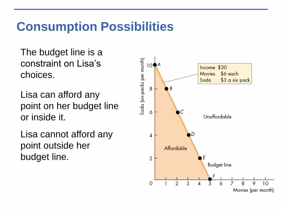
Consumption Possibilities
The budget line is a
constraint on Lisa’s
choices.
Lisa can afford any
point on her budget line
or inside it.
Lisa cannot afford any
point outside her
budget line.

Consumption Possibilities
The Budget Equation
We can describe the budget line by using a budget
equation.
The budget equation states that
Expenditure = Income
Call the price of soda PS, the quantity of soda QS, the price
of a movie PM, the quantity of movies QM, and income Y.
Lisa’s budget equation is:
PSQS + PMQM = Y.

Consumption Possibilities
A household’s real income is the income expressed as a
quantity of goods the household can afford to buy.
Lisa’s real income in terms of soda is the point on her
budget line where it meets the y-axis.
A relative price is the price of one good divided by the
price of another good.
Relative price is the magnitude of the slope of the budget
line.
The relative price shows how many sodas must be
forgone to see an additional movie.
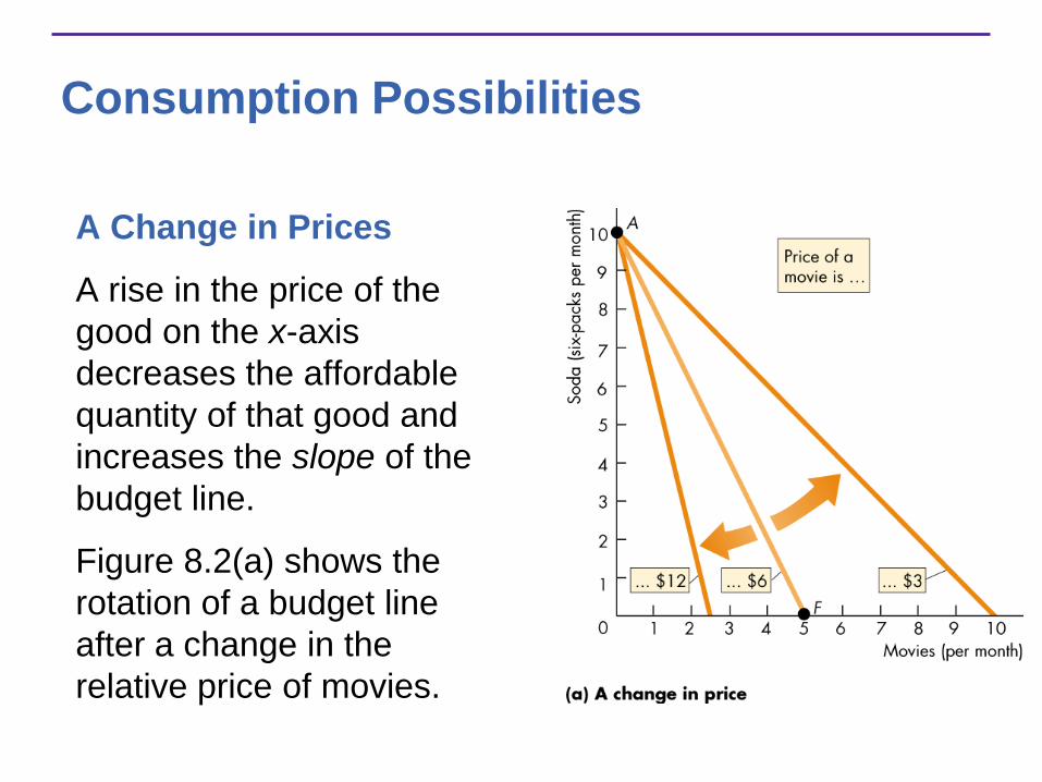
Consumption Possibilities
A Change in Prices
A rise in the price of the
good on the x-axis
decreases the affordable
quantity of that good and
increases the slope of the
budget line.
Figure 8.2(a) shows the
rotation of a budget line
after a change in the
relative price of movies.
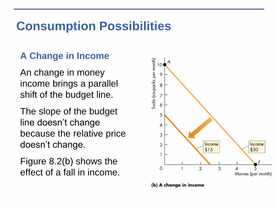
Consumption Possibilities
A Change in Income
An change in money
income brings a parallel
shift of the budget line.
The slope of the budget
line doesn’t change
because the relative price
doesn’t change.
Figure 8.2(b) shows the
effect of a fall in income.
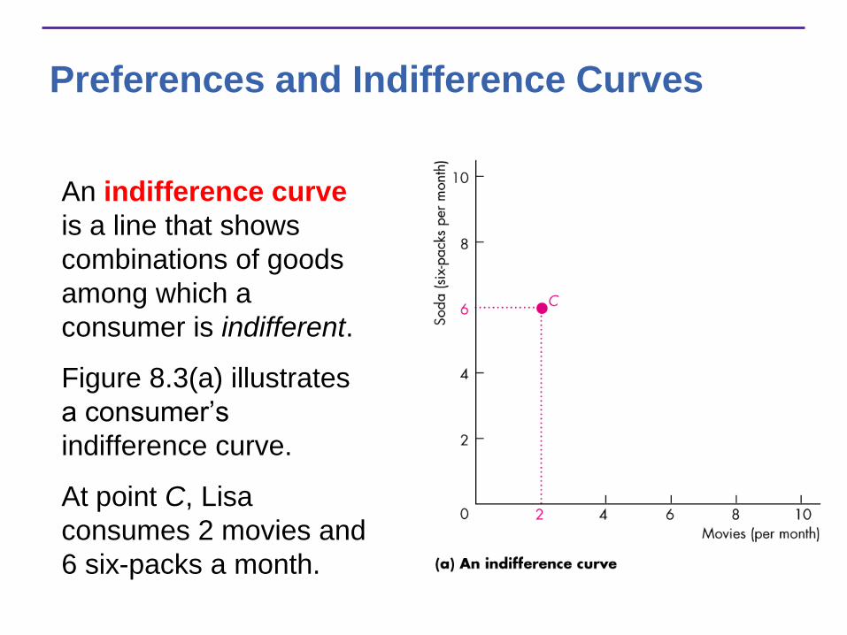
Preferences and Indifference Curves
An indifference curve
is a line that shows
combinations of goods
among which a
consumer is indifferent.
Figure 8.3(a) illustrates
a consumer’s
indifference curve.
At point C, Lisa
consumes 2 movies and
6 six-packs a month.
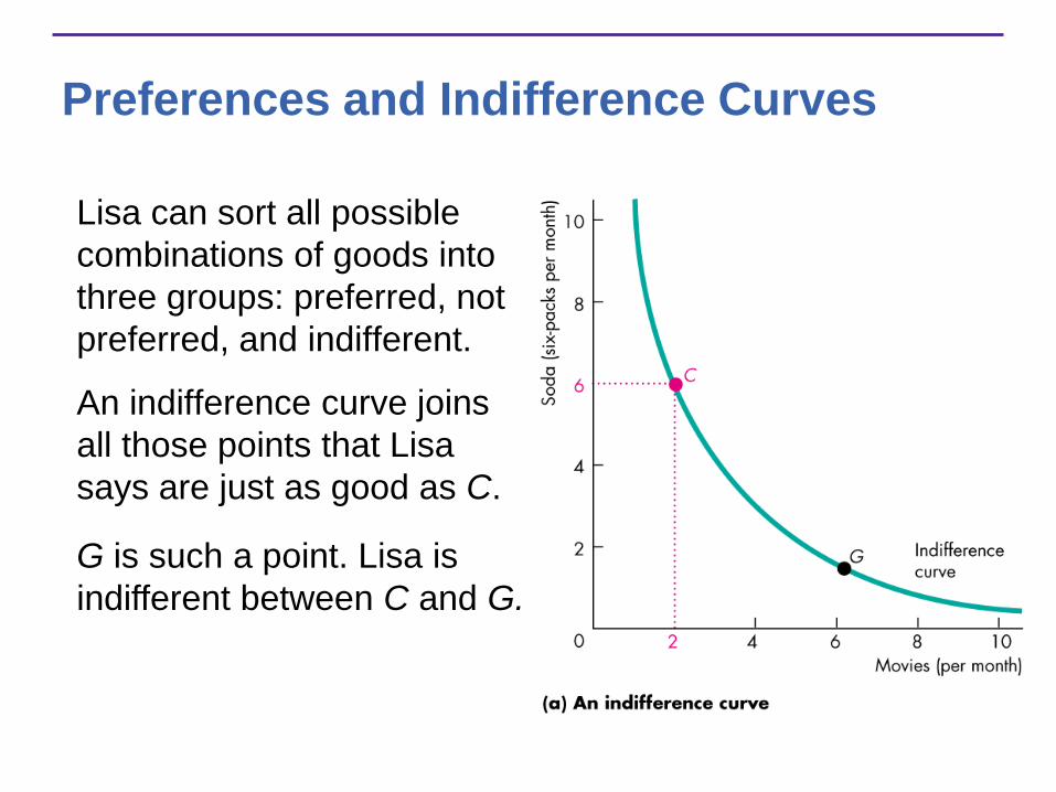
Preferences and Indifference Curves
Lisa can sort all possible
combinations of goods into
three groups: preferred, not
preferred, and indifferent.
An indifference curve joins
all those points that Lisa
says are just as good as C.
G is such a point. Lisa is
indifferent between C and G.
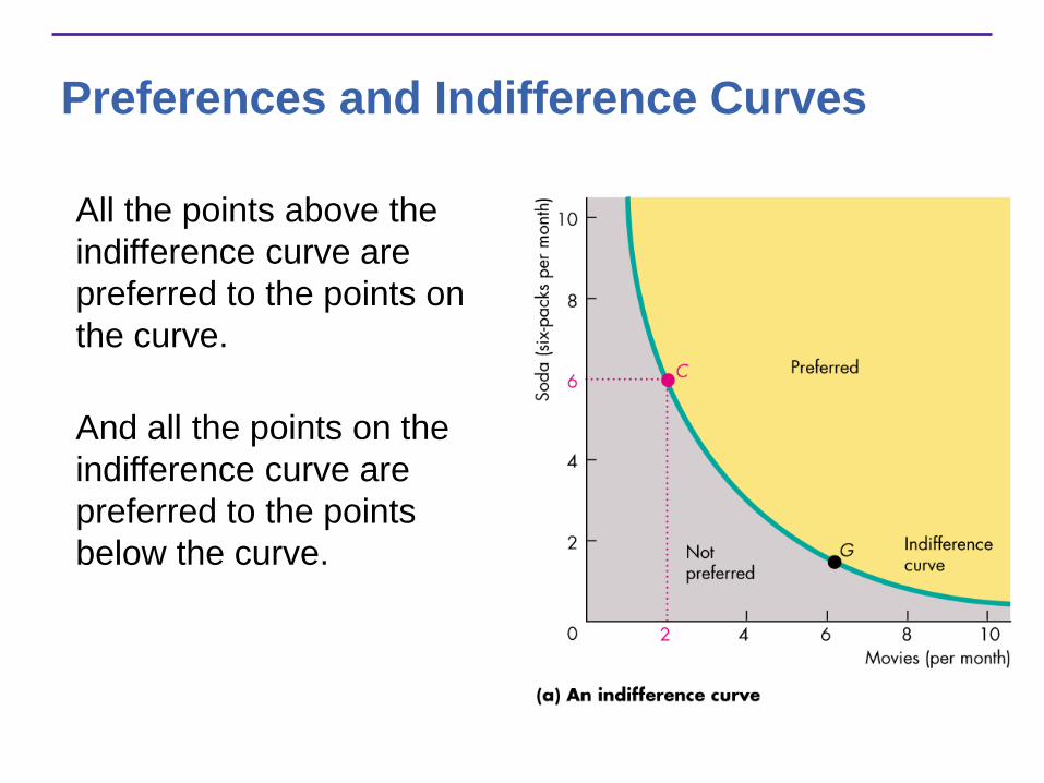
Preferences and Indifference Curves
All the points above the
indifference curve are
preferred to the points on
the curve.
And all the points on the
indifference curve are
preferred to the points
below the curve.
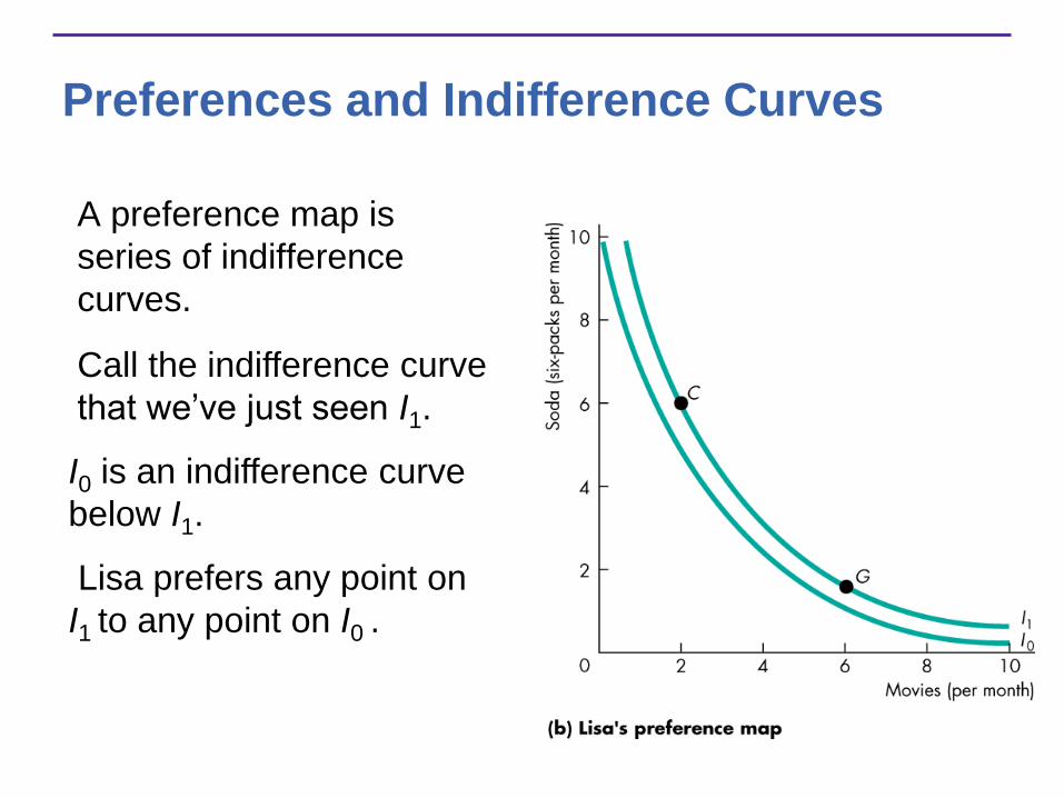
Preferences and Indifference Curves
A preference map is
series of indifference
curves.
Call the indifference curve
that we’ve just seen I1.
I0 is an indifference curve
below I1.
Lisa prefers any point on
I1 to any point on I0 .

Preferences and Indifference Curves
I2 is an indifference curve above I1.
Lisa prefers any point on I2
to any point on I1 .
For example, Lisa prefers
point J to either point C or
point G.

Preferences and Indifference Curves
Marginal Rate of Substitution
The marginal rate of substitution, (MRS) measures the
rate at which a person is willing to give up good y, (the
good measured on the y-axis) to get an additional unit of
good x (the good measured on the x-axis) and at the same
time remain indifferent (remain on the same indifference
curve).
The magnitude of the slope of the indifference curve
measures the marginal rate of substitution.
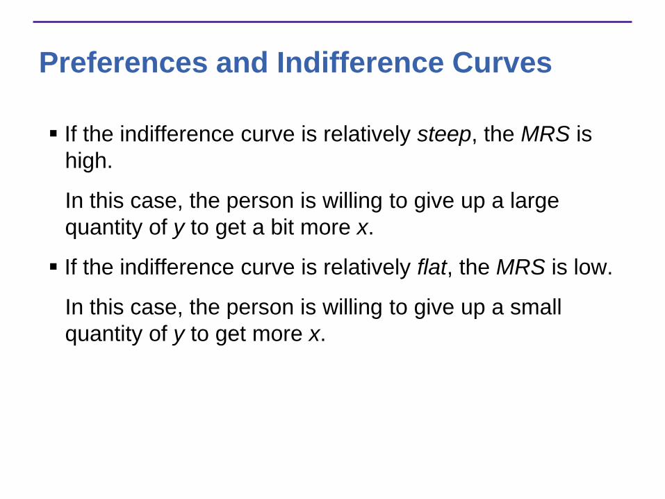
Preferences and Indifference Curves
If the indifference curve is relatively steep, the MRS is
high.
In this case, the person is willing to give up a large
quantity of y to get a bit more x.
If the indifference curve is relatively flat, the MRS is low.
In this case, the person is willing to give up a small
quantity of y to get more x.
Preferences and Indifference Curves
A diminishing marginal rate of substitution is the key
assumption of consumer theory.
A diminishing marginal rate of substitution is a general
tendency for a person to be willing to give up less of good
y to get one more unit of good x, and at the same time
remain indifferent, as the quantity of good x increases.

Preferences and Indifference Curves
Figure 8.4 shows the
diminishing MRS of
movies for soda.
At point C, Lisa is willing
to give up 2 six-packs to
see one more movie—her
MRS is 2.
At point G, Lisa is willing
to give up 1/2 a six-pack
to see one more movie—
her MRS is 1/2.
Preferences and Indifference Curves
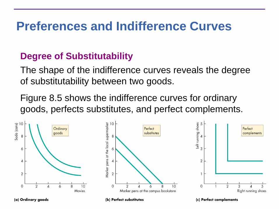
Degree of Substitutability
The shape of the indifference curves reveals the degree
of substitutability between two goods.
Figure 8.5 shows the indifference curves for ordinary
goods, perfects substitutes, and perfect complements.

Predicting Consumer Behavior
The consumer’s best affordable point is:
On the budget line
On the highest attainable indifference curve
Has a marginal rate of substitution between the two
goods equal to the relative price of the two goods
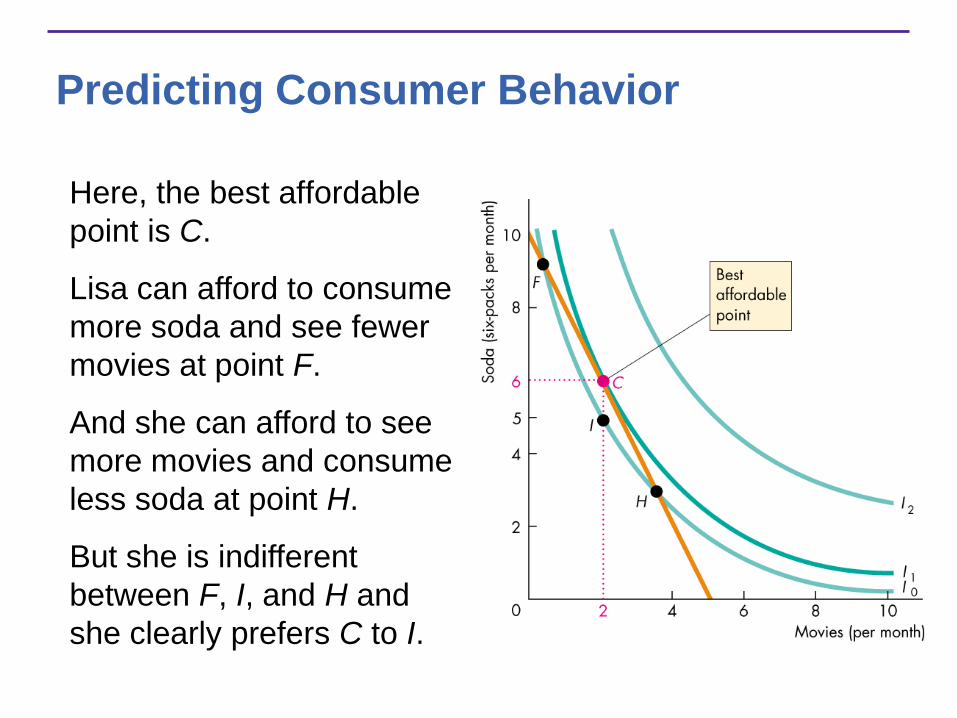
Predicting Consumer Behavior
Here, the best affordable
point is C.
Lisa can afford to consume
more soda and see fewer
movies at point F.
And she can afford to see
more movies and consume
less soda at point H.
But she is indifferent
between F, I, and H and
she clearly prefers C to I.

Predicting Consumer Behavior
At point F, Lisa’s MRS is
greater than the relative
price.
At point H, Lisa’s MRS is
less than the relative price.
At point C, Lisa’s MRS is
equal to the relative price.

Predicting …
A Change in Price
The effect of a change in the
price of a good on the quantity of
the good consumed is called the
price effect.
Figure 8.7 illustrates the price
effect and shows how the
consumer’s demand curve is
generated.
Initially, the price of a movie is $6
and Lisa consumes at point C in
part (a) and at point A in part (b).

Predicting …
The price of a movie then
falls to $3.
The budget line rotates
outward.
Lisa’s best affordable point is
now J in part (a).
In part (b), Lisa moves to point
B, which is a movement along
her demand curve for movies.

Predicting …
A Change in Income
The effect of a change in
income on the quantity of a
good consumed is called the
income effect.
Figure 8.8 illustrates the effect
of a decrease in Lisa’s income.
Initially, Lisa consumes at point
J in part (a) and at point B on
demand curve D0 in part (b).

Predicting …
Lisa’s income decreases and
her budget line shifts leftward
in part (a).
Her new best affordable point
is K in part (a).
Her demand for movies
decreases, shown by a leftward
shift of her demand curve for
movies in part (b).

Predicting Consumer Behavior
Substitution Effect and Income Effect
For a normal good, a fall in price always increases the
quantity consumed.
We can prove this assertion by dividing the price effect in
two parts:
Substitution effect
Income effect

Predicting Consumer Behavior
Initially, Lisa has an
income of $30, the price of
a movie is $6, and she
consumes at point C.
Lisa’s best affordable point
is then J.
The move from point C to
point J is the price effect.
The price of a movie falls
from $6 to $3 and her
budget line rotates outward.

Predicting Consumer Behavior
We’re going to break the
move from point C to
point J into two parts.
The first part is the
substitution effect and
the second is the
income effect.

Predicting Consumer Behavior
Substitution Effect
The substitution effect is the effect of a change in price on the quantity bought when the consumer remains indifferent between the original situation and the new situation.
Predicting Consumer Behavior
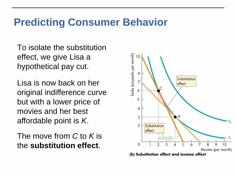
To isolate the substitution
effect, we give Lisa a
hypothetical pay cut.
Lisa is now back on her
original indifference curve
but with a lower price of
movies and her best
affordable point is K.
The move from C to K is
the substitution effect.
Predicting Consumer Behavior
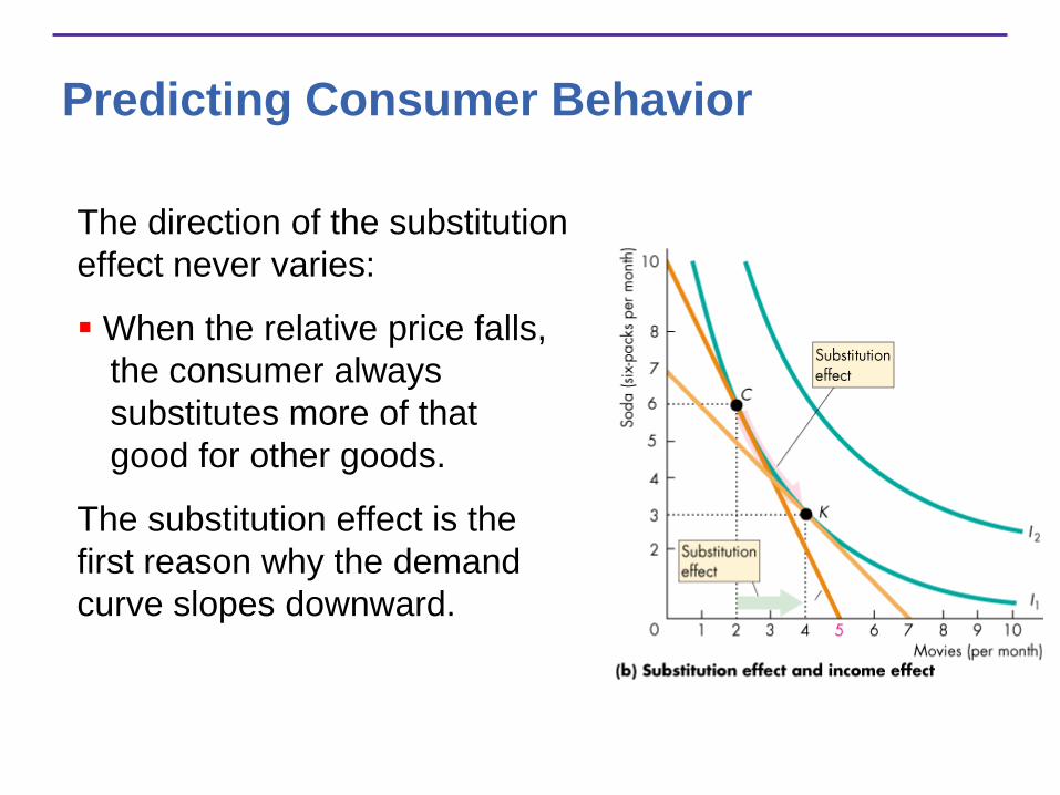
The direction of the substitution
effect never varies:
When the relative price falls,
the consumer always
substitutes more of that
good for other goods.
The substitution effect is the
first reason why the demand
curve slopes downward.

Predicting Consumer Behavior
Income Effect
To isolate the income effect,
we reverse the hypothetical
pay cut and restore Lisa’s
income to its original level
(its actual level).
Lisa is now back on
indifference curve I2 and her
best affordable point is J.
The move from K to J is
the income effect.

Predicting Consumer Behavior
For Lisa, movies are a normal
good.
When her income increases,
she sees more movies—the
income effect is positive.
For a normal good, the
income effect reinforces the
substitution effect and is the
second reason why the
demand curve slopes
downward.

Predicting Consumer Behavior
Inferior Good
For an inferior good, when income increases, the
quantity bought decreases.
For an inferior good, the income effect works against
the substitution effect.
So long as the substitution effect dominates, the
demand curve still slopes downward.
Predicting Consumer Behavior
If the negative income effect is stronger than the
substitution effect, a lower price for inferior goods brings a
decrease in the quantity demanded—the demand curve
slopes upward!
This case does not appear to occur in the real world.
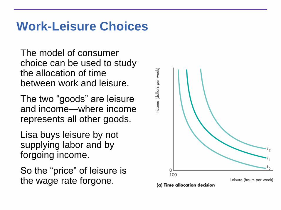
Work-Leisure Choices
The model of consumer choice can be used to study the allocation of time between work and leisure.
The two “goods” are leisure and income—where income represents all other goods.
Lisa buys leisure by not supplying labor and by forgoing income.
So the “price” of leisure is the wage rate forgone.
Work-Leisure Choices
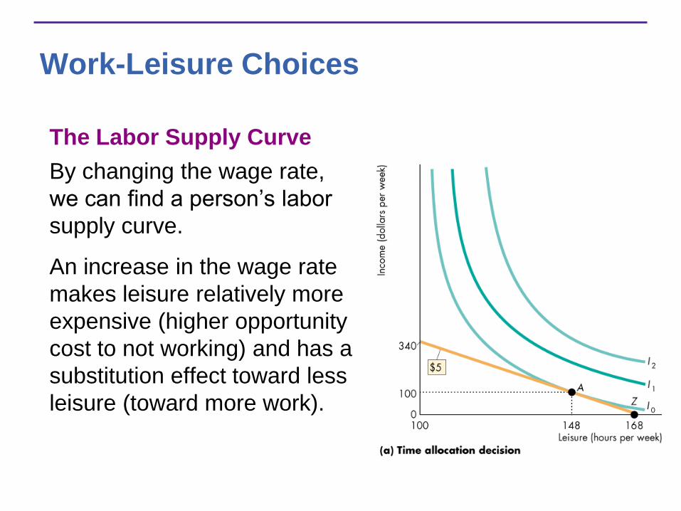
The Labor Supply Curve
By changing the wage rate,
we can find a person’s labor
supply curve.
An increase in the wage rate
makes leisure relatively more
expensive (higher opportunity
cost to not working) and has a
substitution effect toward less
leisure (toward more work).
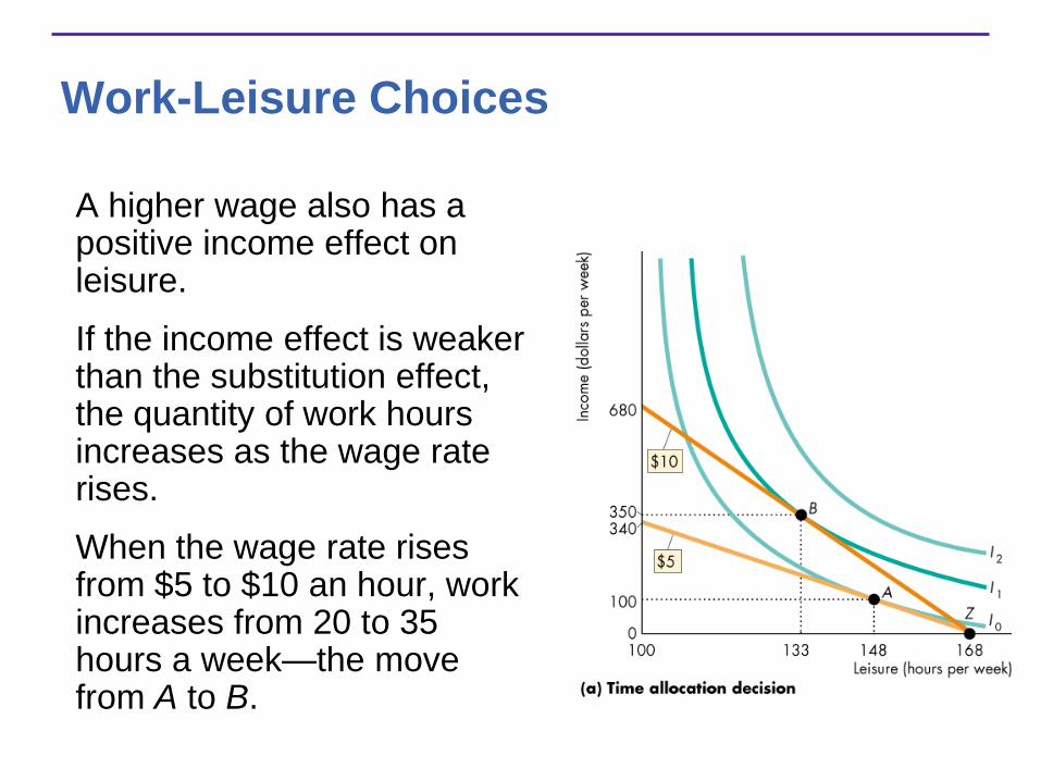
Work-Leisure Choices
A higher wage also has a positive income effect on leisure.
If the income effect is weaker than the substitution effect, the quantity of work hours increases as the wage rate rises.
When the wage rate rises from $5 to $10 an hour, work increases from 20 to 35 hours a week—the move from A to B.

Work-Leisure Choices
But if the income effect is
stronger than the substitution
effect, the quantity of work
hours decreases as the wage
rate rises.
When the wage rate rises
from $10 to $15 an hour,
work decreases from 35 to 30
hours a week —the move
from B to C.
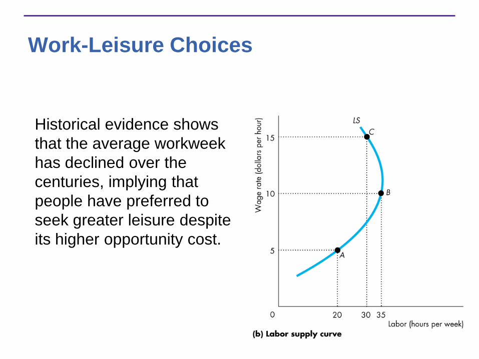
Work-Leisure Choices
Historical evidence shows
that the average workweek
has declined over the
centuries, implying that
people have preferred to
seek greater leisure despite
its higher opportunity cost.