Precision Agriculture Technology Adoption...

Precision Agriculture Technology Adoption for Cotton Production

Paxton, Kenneth W.; Mishra, Ashok K.; Chintawar, Sachin; Larson, James A.; Roberts, Roland

K.; English, Burton C.; Lambert, Dayton M.; Marra, Michele C.; Larkin, Sherry L.; Reeves, Jeanne M.; Martin, Steven W.

Correspondence to:

Ashok K. Mishra Associate Professor

Department of Agricultural Economics and Agribusiness Louisiana State University AgCenter

211 Ag. Admin. Bldg. Baton Rouge, LA 70803

Tel: 225-578-0262 Fax: 225-578-2716

E-mail: [email protected]

Selected Paper prepared for presentation at the Southern Agricultural Economics Association Annual Meeting, Orlando, FL, February 6-9, 2010

Copyright 2010 by Paxton et al.,. All rights reserved. Readers may make verbatim copies of this document for non-commercial purposes by any means, provided that this copyright notice appears on all such copies.


Kenneth W. Paxton, Professor

Louisiana State University AgCenter Baton Rouge, LA 70803

Phone: 225-578-2763 E-mail: [email protected]

Ashok K. Mishra, Associate Professor Louisiana State University AgCenter

Baton Rouge, LA 70803 Phone: 225-578-0262


Sachin Chintawar Graduate Research Assistant

Louisiana State University AgCenter Baton Rouge, LA 70803


Roland K. Roberts, Professor The University of Tennessee

308B Morgan Hall, 2621 Morgan Circle Knoxville, TN 37996-4518


James A. Larson, Associate Professor The University of Tennessee

308G Morgan Hall, 2621 Morgan Circle Knoxville, TN 37996-4518

Phone: 865-974-3716 Email: [email protected]

Burton C. English, Professor The University of Tennessee

308C Morgan Hall, 2621 Morgan Circle Knoxville, TN 37996-4518

Phone: 865-974-3716 E-mail:[email protected]

Dayton M. Lambert, Assistant Professor

The University of Tennessee 321C Morgan Hall, 2621 Morgan Circle

Knoxville, TN 37996-4518 Phone: 865-974-3716

Email: [email protected]

Michele C. Marra, Professor, North Carolina State University

Box 8109 Raleigh, NC 27695-8109

Phone: 919-515-6091 Email: [email protected]

Sherry L. Larkin, Associate Professor

University of Florida, P.O. Box 110240

Gainesville, FL 32611-0240 Phone: (352) 392-1845 Email: [email protected]

Jeanne M. Reeves, Director, Agricultural Research, Cotton Incorporated

6399 Weston Parkway Cary, NC 27513


Steven W. Martin, Associate Professor and

Extension Economist Delta Research and Extension Center

Mississippi State University Stoneville, MS 38776 Phone: 662-686-3234



Abstract

Many studies on the adoption of precision technologies have generally used logit models to explain the adoption behavior of individuals. This study investigates factors affecting the number of specific types of precision agriculture technologies adopted by cotton farmers. Particular attention is given to the influence of spatial yield variability on the number of precision farming technologies adopted, using a Count data estimation procedure and farm-level data. Results indicate that farmers with more within-field yield variability adopted a larger number of precision agriculture technologies. Younger and better educated producers and the number of precision agriculture technologies were significantly correlated. Finally, farmers using computers for management decisions also adopted a larger number of precision agriculture technologies.

Keywords: precision technologies, Poisson, Negative Binomial, count-data method, GIS, education, cotton


Introduction Precision agriculture (PA) or precision farming (PF) generally refers to a system that assesses

within-field variability in both soil and crops. Information gathered in these assessments is then

used to develop site specific management practices that optimize crop production. A wide variety

of technologies are used in collecting site specific data and deploying the site specific

management practices. Some of these technologies have been commercially available since the

late 1980s and includes yield monitoring/mapping, variable rate application, and a host of other

spatial management technologies. The adoption of precision agriculture technologies is

somewhat different from many other technologies introduced in agricultural production. A major

difference is the fact that precision agriculture technologies consist of a complex set of

technologies, each with a specific purpose (Lowenberg-DeBoer 1998, Khanna, Epouhe, and

Hornbaker 1999, Khanna 2001). Therefore, farmers may adopt one or more technologies and

evaluate those before adopting additional technologies (Byerlee and de Polanco 1986; Leathers

and Smale 1991). The most recent studies have examined the adoption of several specific

technologies (Daberkow et al. 2002; Daberkow and McBride 2000; Fountas et al. 2003; Griffin

et al. 2004).

The adoption of PA technology in cotton production has been somewhat different than in

grain crops, because cotton yield monitors were not available until the late 1990s while yield

monitors for combines were introduced in the late 1980s (Griffin et al., 2004). The unavailability

of yield monitors influenced cotton producers to use grid soil sampling or other soil mapping

techniques as an entry point for adopting precision agriculture technology (Walton et al., 2008).

Since the introduction of the cotton yield monitor, several studies have examined the adoption of

precision agriculture technologies in cotton production (Roberts et al. 2004; Banerjee et al 2008;

Larson et al. 2008; Walton et al. 2008). Most of these studies estimate the likelihood of adopting

utilizing a logit model.

This study is unique in determining the influence of various farm, operator, and location

attributes on the number of precision farming technologies adopted by farmers. Particular

attention is given to the role of spatial yield variability. The technologies evaluated include yield

mapping, variable rate application, yield monitoring, grid sampling, and others. Because

precision agriculture consists of a set of technologies that may be adopted sequentially, one must

go beyond the simple binomial logit to understand past growth and to predict future growth in

adoption. This information is critical to (1) the development of educational programs addressing

precision agriculture, and (2) anticipation of future demand by cotton producers, crop

consultants, dealerships, and equipment manufacturers.

Literature Review

Precision agriculture (PA) is an approach to re-organize the total system of agriculture

production towards one that uses fewer inputs, is more efficient, and is sustainable. The early

literature provides broad agreement that profitability and/or input cost reduction from new

innovation or technology adoption plays a key role in the extent and rate of technology adoption

(Feder et al. 1985; Rogers 1995). In 1997, Whelan et al. concluded that the desire to respond to

production variability on a fine-scale has become the goal of precision agriculture. Swinton and

Lowenberg-DeBorer (1998) conclude that because precision farming practices are site-specific,

their profitability potential is also site-specific. In a follow-up study, Lowenberg-DeBorer (1999)

showed that site-specific farming, to which most of PA technologies is geared, could reduce

whole-field yield variability. Finally, Zhang et al. (2002), while assessing the role of precision

agriculture throughout the world, concluded that the success of precision agriculture technologies

will have to be measured by economic and environmental gains.

It has long been recognized that the advancement of the PA approach depends on the

emergence and convergence of several technologies (Shibusawa 1998), including geographic

information systems (GIS), Global Positioning System (GPS), in-field remote sensing, automatic

controls, miniaturized computer components, mobile computing, and telecommunications

(Gibbons 2000). Erickson and Lowenberg-DeBorer (2000) conclude that yield monitors, GPS

receivers, and GIS mapping are useful to maintain precise records of the location, planted acres,

and yield of crops. In 2002, Cox reviewed developments in information technology that are

contributing to global improvements in crop and livestock production. In a case study of six

leading early adopters of precision agriculture technologies, Batte and Arnholt (2003) point out

that precision farming has the potential to help farmers improve input allocation decisions. The

specific role of GIS and GPS in precision farming was explored by Nemenyi et al. (2003) and

they concluded that GIS maps created by complex computing backgrounds are essential in

making effective agrotechnological decisions.

While both the potential for PA to improve sustainability (fiscal and environmental) and

the need for continual advancements in a suite of technology are critical factors to the ultimate

success of this farming approach, the behavior of individual farmers in adopting new

technologies is also of paramount importance. To that end, Roberts et al. (2000) found that the

profitability of precision farming – as assessed by cotton farmers with varying degrees of

adopting a suite of technologies – depends immensely on the degree of spatial variability of soil

attributes and yield response. In the case of precision agriculture technologies, record keeping

and documentation functions inherent in PA systems may help farmers increase yields and hence

profits. In studying adoption of PA technologies in the U.S., Daberkow and McBride (2003)

noted that farm size, human capital, risk preference, off-farm labor supply, location, and tenure

are some of the factors that affect adoption. With respect to human capital in particular,

Daberkow and McBride (2003) also noted that human capital could take the form of familiarity

with related technologies. The authors show that farmers who kept computerized financial

records are more likely to be associated with PA technologies.

In our study we advance the literature related to PA by focusing on spatial yield

variability and how that farm characteristic relates to the number of PA technologies adopted.

The focus on explaining the number of PA technologies is unique to the adoption literature and is

ideally suited to the case study, which uses a sample of cotton farmers in the Southern U.S. This

is because the production of cotton can employ a sufficient number of technologies to support

the empirical analysis.

Empirical Approach

In some cases, such as number of patents (Cincera, 1997), visits to doctors (Cameron and Trivedi

2009), and number of foreign domestic investment firms (Gopinath and Vasavada, 1999) the

count is the variable of ultimate interest. In other cases, such as medical expenditures (Cameron

and Trivedi, 2009) and the variable of ultimate interest is the continuous variable. In our case,

the data are the count of the number of precision technologies adopted by each cotton farmer.

Cameron and Trivedi (2006) point out that in such cases count data models are appropriate. To

analyze the effects of various farm, operator, and regional characteristics on the number of

precision technologies (such as yield monitors with GPS, yield monitors without GPS, soil

sampling grid, soil sampling zone, aerial photos, satellite images, soil survey maps, and handheld

GPS/PDAs), we use the method employed in patent literature (e.g., Hausman et al., (1984);

Cameron and Trivedi (1986) ; Cincera,(1997)).

In our study, the number of precision technologies adopted by a cotton farmer is a

function of a set of independent variables ( Xi ):

0ln( )i iXλ α β ′= + (1)

where λi is the number of precision technologies adopted by farm operator i. Data on the

number of precision technologies used constitute a nonnegative, integer-valued, random variable.

Several authors (e.g., Hausman et al.; Cameron and Trivedi; Cincera) have presented and

discussed count data models as an alternative method to the classical linear model.1 In the count

data models, the primary variables of interest are event counts. We consider the Poisson and the

negative binomial distributions, which are within the linear exponential family, for analyzing the

number of precision technologies used by farm operators. We will briefly describe the Poisson

and negative binomial models below.

Poisson Model

Let Yi be the observed event count (number of precision technologies used) for the ith farm

operator. The Yi are assumed to be independent and have a Poisson distribution. The parameters

β depend on a set of explanatory variables ( iX ), which are the factors affecting the number of

precision technologies used by a farm operator.

( ) ( )| exp , =1... ,i i i iE Y X X i Nλ β ′= = (2)

where iλ is the intensity-of-rate parameter when referring to the Poison distribution as [ ]ip λ .

The probability density function for the Poisson model is:

1 See Winkelmann and Zimmermann for a recent overview of count data models.

( ) ( )Pr , 0,1,2.....,!

i iYi

i i ii

eY y f Y YY

λ λ−⎡ ⎤= = = =⎢ ⎥

⎣ ⎦ (3)

The first two moments of [ ]ip λ are [ ]E Y λ= and [ ]V Y λ= ; the Poisson specification assumes

equal mean and variance. Overdispersion has a qualitatively similar consequence to failure of the

homoscedasticity assumption in the linear regression model. For linear models

with [ ]E |Y X X β= , the estimated coefficients β are interpreted as the effect of a one unit

change in regressors on the conditional mean.

The Negative Binomial Model

A drawback to the Poisson specification is the assumption of equal mean and variance of Yi, a

testable hypothesis. In the negative binomial model, which is more flexible than the Poisson,

iλ is assumed to follow a gamma distribution with parameters ( ),γ δ , where ( )β=γ iX exp and

δ is common across firms. The gamma distribution for iλ is integrated by parts to obtain a

negative binomial distribution with parameters ( ),iγ δ . Specifically,

( ) ( )

( )( ) ( ) ( )

0

1Pr f

= 11 1

i i

ii

Yi i i i

i

i i

i i

Y e dY

λ

γλ

λ λ λ

γ λ δ δγ λ δ

∞−

−

=

Γ + ⎛ ⎞ +⎜ ⎟Γ Γ + +⎝ ⎠

∫. (4)

The above framework suggests that the number of precision technologies used by a cotton

producer is expressed as a function of various farm, operator, household, and regional

characteristics. Specifically, exp( )i iXλ β ′= where Xi is a set of explanatory variables such as age

and education of the operator, farming experience, farm size, yield index, and state dummies. A

subsequent question then arises as to which model (Poisson or negative binomial) is more

appropriate. Cameron and Trivedi (2009) proposed a number of tests for the over- or under

dispersion in the Poisson regression model. They test the underlying assumption of mean-

variance equality, where the null hypothesis, ( )1 : Var i iH Y μ= is compared with the alternative

hypothesis, ( ) ( )*1 : Var i i iH Y gμ α μ= + . The function g(.) is a specified function that maps

from R+ to R+. Tests for overdispersion or underdispersion are tests of whether 0 =α .2 We use a

similar test in our study. The marginal effect of a change in an independent variable on the

conditional mean of the dependent variable was calculated using the STAT software. Cameron

and Trivedi (2009, pp. 562-566) provide a detailed explanation and interpretation of marginal

effects of the Poisson and negative binomial models. Specifically, Cameron and Trivedi (2009)

point out that the marginal effect of the ith variable (MEi)= ( )| * iE y x β .

The choice of attributes associated with the number of precision technologies used is

guided by human capital theory, farm and production characteristics, and other adoption models.

Nelson and Phelps (1980), Khaldi (1979), and Wozniak (1989) use education as a measure of

human capital to reflect the ability to innovate (either technology or insurance). In addition, other

factors affecting the adoption of precision farming technologies are driven by the literature

(Feder et al., 1985; Rogers, 1995; Deberkow and McBride, 2003). In our model, we use

financial, location, and the physical attributes of the farm firm that may also influence

profitability and, ultimately the adoption of precision agriculture technologies (Deberkow and

McBride, 2003).

2 Tests for over dispersion and under dispersion are important “Failure has consequences similar to those of heteroskedasticity in Linear Regression Model” Cameron and Trivedi (1990).

Data

Data for this analysis was obtained from a survey of cotton producers in the Southeastern part of

the United States (Alabama, Arkansas, Florida, Georgia, Louisiana, Mississippi, Missouri, North

Carolina, South Carolina, Tennessee, and Virginia). The survey utilized a questionnaire to obtain

information about producer attitudes toward and use of precision agriculture technologies.

Following Dillman’s (1978) general mail survey procedures, the questionnaire, a postage-paid

return envelope, and a cover letter were sent to each producer. A reminder post card was sent one

week after the initial mailing. Three weeks later a second mailing was sent to those not

responding to the original mailing and reminder. The mailing list of potential cotton producers

for the 2003-04 crop year was obtained from the Cotton Board in Memphis, Tennessee (Skorupa,

2004). The survey was mailed in January and February of 2005. Of the 12,245 questionnaires

mailed, 18 were returned undeliverable, 184 respondents were no longer cotton producers, and

1,215 respondents provided useable information for a response rate of 10 percent. Figure 1

provides information of the distribution of the number of precision technologies adopted by

cotton farmers in 2003-04. About 39 percent of farmers reported using one or more precision

technologies; additionally about 9 percent of cotton farmers have used 3 or more precision

technologies.

Table 1 provides definitions and summary statistics for the variables used in empirical

model. The average cotton farmer in the Southern United States is 49 years of age and has 14

years of schooling. An average cotton farmer has about 26 years of farming experience and

receives 73 percent of household income from farming. The modal cotton precision farmer used

one precision technology (Figure 1) while average precision technology use was 0.85 (Table 1).

Additionally, 54 percent of cotton farmers thought precision technologies would be profitable in

the near future. About 18 percent of the farms were located in Georgia or North Carolina

compared to 13 and 12 percent in Mississippi and Alabama. Arkansas was used as the

benchmark state in the regression.

Results

First the choice of Poisson and negative binomial model was tested and results indicated that the

null hypothesis of equal mean and variance was rejected. The test statistics (overdispersion) was

significant at the 1 percent level (Table 2, last row). Therefore, Table 2 only presents the

parameter estimates from the negative binomial model and their marginal effects. The estimated

model fits reasonably well as indicated by the 70-pecent correlation between observed and

predicted values (Table 2).

Results suggest that an additional year of age (OP_AGE) is associated with 2 percent

fewer precision technologies adopted by farmers (Table 2, 3rd column)3. This finding is

consistent the adoption literature (Feder et al., 1985; Daberkow and McBride, 2003) and with the

hypothesis that older farmers are less likely to adopt new technologies because of a lower

expected payoff from a shortened planning horizon over which the benefits can accumulate.

Results suggest that educational attainment (OP_EDUC) positively influences the

number of precision technologies adopted (Table 2). One additional year of schooling is

associated with approximately an 8 percent increase in the number of precision technologies

adopted. A plausible explanation is that many educated farmers are young and are often

hypothesized to be more willing to innovate and adopt new technologies that reduce time spent

3 Cameron and Trivedi (2009) show that another way of interpreting the marginal effect is to obtain exponentiated coefficients ( eβ ), thus one additional year in age is associated with number of PA technologies decreasing by 1.02. The Exponentiated coefficient applies to any Maximum Likelihood estimation (see Cameron and Trivedi, 2009, page: 558-564).

farming (Mishra et al., 2002). In particular, Mishra et al (2002) point out that many young

farmers are more educated and often have off-farm jobs. Our results are also consistent with the

findings of Daberkow and McBride (2003) who investigated the impact of education, in addition

to other factors, on PA technology adoption.

Mishra, El-Osta, and Johnson (1999) concluded that cash grain farms who kept

computerized financial records were more likely to be successful. In a similar vein, computer use

for financial record keeping may be an indicator of preferences toward using information

technology tools for farm management. The marginal effect of COMPFARM4 indicates that

farmers who use computers for farm management increase the number of PA technologies by 43

percent.

The 2005 Southern cotton survey queried farmers on farm planning. In particular, farmers

were asked if they planned to expand the size of their operation or acquire additional assets to

generate additional income (FARMPLAN), and 72 percent responded positively. Cotton farmers

who planned to expand their operations decreased the number of precision technologies adopted

by 21 percent. A possible explanation is that farmers planning to expand their operations may

use their resources (particularly income and labor) to purchase additional land rather than

investing it in an additional PA technology.

Future expectation of increased profits through precision technologies

(FUTURE_ADOPT) has a positive impact on the number of precision technologies adopted by

cotton farmers. The marginal effect for this variable suggests that farmers who thought precision

technologies would be profitable in the future increased the number of precision technologies

adopted by 42 percent.

4 Potential endogeneity of this variable was test using the Hausman test. Based on the statistics the null hypothesis of endogeneity was rejected.

As the share of farm income in total household income (F_INCOME) increases, the number

of precision technologies adopted by farmers increases by only 0.2 percent. This result is

consistent with the tradeoff between on-farm and off-farm labor requirements. A lower

percentage of household income earned from farming implies more household labor is employed

off the farm, and less household labor is available to evaluate and implement new technologies.

An important finding is that spatial yield variability5 (LN_SPYVAR) has a positive

impact on the number of PA technologies adopted by cotton farmers. The marginal effect

indicates that a 1 percent increase in spatial yield variability is associated with 7 percent increase

in the number of precision technologies adopted by cotton farmers in the South.

Finally, location of the farm has an important role in the number of precision

technologies adopted by cotton farmers. Cotton farmers in Mississippi and Missouri are likely to

use a higher number of PA technologies when compared to farmers in the benchmark state of

Arkansas (Table 2), while cotton farmers in Florida are likely to use fewer precision technologies

compared to farmers in Arkansas.

Conclusions This study examined the effects of various farm, operator, and regional characteristics on the

number of precision agriculture technologies adopted by cotton farmers in the southeast. A

negative binomial count model was used to analyze data collected through a 2005 survey of

cotton producers in the southeast United States. This study contributes to the literature in two

ways. First, this study uses count data estimation procedure to examine the impact of various

factors on the number of precision agriculture technologies adopted by cotton farm operators.

5 We use Larson and Roberts (2004) method to calculate spatial variability. The log of spatial yield variability is used to scale down the variable.

Second, it incorporates a measure of within-field yield variability as a factor influencing the

number of technologies adopted.

Results from this study indicate that the number of precision agriculture technologies

employed by producers is positively correlated with the educational level of the producer and

negatively correlated with the age of the operator. These results suggest that younger, better

educated producers adopt a larger number of precision agriculture technologies. Farmers using

computers for management decisions also adopted a larger number of precision agriculture

technologies. These results suggest that targeting these groups for educational programs would

increase the probabilities of success for those programs. Results of this analysis demonstrated

that farmers with more within-field yield variability adopted a larger number of precision

agriculture technologies. Within-field yield variability has long been thought of as the primary

driver of precision agriculture adoption. Results of this study confirm this long held belief.

Overall, the results obtained here help identify groups of cotton producers that are more likely to

be responsive to precision agriculture technology educational programs. These results also

identify those groups where educational programs may be used to expand precision agriculture

technology adoption.

References Batte, M. and M. W. Arnholt. “Precision Farming Adoption and Use in Ohio: Case Studies of Six Leading-edge Adopters.” Computers & Electronics in Agriculture 38(2003), 125-129. Banerjee, S., S.W. Martin, R.K. Roberts, S.L. Larkin, J.A. Larson, K.W. Paxton, B.C. English, M.C. Marra, and J.M. Reeves.2008. "A Binary Logit Estimation of Factors Affecting Adoption of GPS Guidance Systems by Cotton Producers." J. Agr. and Applied Econ. 40(2008):335-344. Byerlee, D. and E. Hesse de Polanco. “Farmers’ Stepwise Adoption of Technological Packages: Evidence from the Mexican Altiplano.” Amer. J. Agr. Econ. 68(1986):519-527. Cameron, A., and P. Trivedi. “Econometric Models Based on Count Data: A Comparison and Implications of Some Estimators and Tests.” Journal of Applied Econometrics 1(January 1986):29-53. Cameron, A., and P. Trivedi. “Regression Based Tests for overdispersion in Poisson Model.” Journal of Econometrics 46(1) (1990): 347-364. Cameron, A., and P. Trivedi. Microeconometrics Using Stata. College Station, TX. Stata Press 2009. Cincera, M. “Patents, R&D, and Technological Spillovers at the Firm Level: Some Evidence from Econometric Count Data Models.” Journal of Applied Econometrics 1(June 1997):265-80. Cox, S. “Information Technology: The Global Key to Precision Agriculture and Sustainability.” Computers & Electronics in Agriculture 36(2002), 93-111. Daberkow, S.G., J. Fernandez-Cornejo, and M. Padgitt. “Precision Agriculture Adoption Continues to Grow.” Pp. 35-38. Agricultural Outlook. Economic Research Service, USDA, Washington, D.C. November 2002. Daberkow, S.G. and W.D. McBride. “Adoption of Precision Agriculture Technologies by U.S. Farmers.” Proceedings of the 5th International Conference on Precision Agriculture, Minneapolis, MN, ASA/CSSA/SSSA, Madison, WI, July 16-19, 2000. Daberkow, S.G. and W.D. McBride. “Farm and Operator Chgaractersitics Affecting the Awareness and Adoption of Precision Agriculture Technologies in the US.” Precision Agriculture, 4(2003): 163-177. Dillman, D.A. Mail and Telephone Surveys: The Total Design Method. New York: John Wiley and Sons, 1978. Erickson, K., Lowenberg-DeBoer, J. (Eds.), Precision Farming Profitability. Purdue University, West Lafayette, IN 2000.

Feder, G., R.J. Just., D. Zilberman. “Adoption of Agricultural Innovations in Developing Countries: A Survey.” Economic Development and Cutltural Change 33(2), 1985: 255-298. Fountas, S., D.R. Ess, C.G. Sorensen, S.E. Hawkins, H.H. Pedersen, B.S. Blackmore, and J. Lowenberg-DeBoer. “Information Sources in Precision Agriculture in Denmark and the USA,” A. Werner and A. Jarfe ed. Precision Agriculture: Proceedings of the 4th European Conference on Precision Agriculture, 2003. Gibbons, G., 2000. Turning a farm art into science--an overview of precision farming. URL: http://www.precisionfarming.com. Griffin, T.W., J. Lowenberg-DeBoer, D.M. Lambert, J. Peone, T. Payne, and S.G. Daberkow. “Adoption, Profitability, and Making Better Use of Precision Farming Data.” Staff Paper #04-06. Department of Agricultural Economics, Purdue University. 2004. Hausman, J. B., H. Hall, and Z. Griliches. “Econometric Models for Count Data with an Application to the Patents-R&D relationship.” Econometrica 52(July 1984): 909-38. Khanna, M. “Sequential Adoption of Site-Specific Technologies and Its Implications for Nitrogen Productivity: A Double Selectivity Model.” Amer. J. Agr. Econ. 83(2001):35-51. Khanna, M., O.F. Epouhe, and R. Hornbaker. “Site-Specific Crop Management: Adoption of components of a Technological Package.” Rev. Agr. Econ. 21(1999):455-472. Larson, J.A., R.K. Roberts, B.C. English, S.L. Larkin, M.C. Marra, S.W. Martin, K.W. Paxton, and J.M. Reeves. 2008. "Farmer Adoption of Remotely Sensed Imagery for Precision Management in Cotton Production." Precision Agriculture 9(2008):195-208. Leathers, H.D. and M. Smale. “Baysian Approach to Explaining Sequential Adoption of Components of a Technological Package.” Amer. J. Agr. Econ. 73(1991):734-742. Roberts, R.K., B.C. English, J.A. Larson, R.L. Cochran, W.R. Goodman, S.L. Larkin, M.C. Marra, S.W. Martin, W.D. Shurley, and J.M. Reeves. “Adoption of Site-Specific Information and Variable-Rate Technologies in cotton Precision Farming.” J. Agr. Appl. Econ. 36(2004):143-158. Lowenberg-Deboer, J. “Risk management potential of precision farming technologies.” Journal of Agricultural and Applied Economics 31 (2): 1999: 275-85. Lowenberg-DeBoer, J. “Adoption Patterns for Precision Agriculture.” Technical Paper No. 982041. Warrendale, PA:Society of Automotive Engineering. 1998. Mishra, Ashok K., M.J. Morehart, Hisham S. El-Osta, James D. Johnson, and Jeffery W. Hopkins. “Income, Wealth, and Well-Being of Farm Operator Households.” Agricultural Economics Report # 812, Economic Research Service, U.S. Department of Agriculture, Washington, D.C. Sept. 2002.

Mishra,A. K., El-Osta, H., Johnson, J. D. “Factors contributing to earnings success of cash grain farms.” J. Agric. Applied Econ. 31(1999): 623–637. Nemenyi, M., P.A. Mesterhazi, Zs. Pecze, and Zs. Stepan. “The Role of GIS and GPS in Precision Farming.” Computers & Electronics in Agriculture 40(2003), 45-55. Roberts, R.K., B.C. English, J.A. Larson, R.L. Cochran, W.R. Goodman, S.L. Larkin, M.C. Marra, S.W. Martin, W.D. Shurley, and J.M. Reeves. “Adoption of Site-Specific Information and Variable-Rate Technologies in Cotton Precision Farming.” J. Agr. and Applied Econ. 36(2004):143-158. Roberts, R.K., English, B.C., Mahajanashetti, S.B. “Evaluating the returns to variable rate nitrogen application.” Journal of Agricultural and Applied Economics 32 (1) 2000, 133-143. Rogers, E.M. Diffusion of Innovations. 4th edition, Free Press, New York, 1995. Shibusawa, S. Precision Farming and Terra-mechanics. Fifth ISTVS Asia-Pacific Regional Conference in Korea, October 20-22, 1998. Skorupa, B. Cotton Board, 871 Ridgeway Loop, Ste. 100. Memphis, TN, 38120-4019. Swinton, S.M., Lowenberg-DeBoer, J., 1998. “Evaluating the profitability of site-specific farming.” Journalof Production Agriculture 11 (4) 1998 439-446. Walton, J.C., Lambert, D.M., Roberts, R.K., Larson, J. A., English, B.C., Larkin, S.L., Martin, S.W., Marra, M.C., Paxton, K.W., and Reeves, J.M. “Adoption and Abandonment of Precision Soil Sampling in Cotton Production.” J. Agr. and Resource Econ. 33(2008):428-448. Whelan, B.M., A.B. McBratney, B.C. Boydell. The Impact of Precision Agriculture. Proceedings of the ABARE Outlook Conference, “The Future of Cropping in NW NSW”, Moore, UK July 1997, p. 5. Winkelmann, R., and K. F. Zimmermann. “Recent Development in Count Data Modelling: Theory and Application.” Journal of Economic Surveys, 9(1995):1-24. Zhang, N., Wang, M. and Wang, N. “Precision agriculture—a worldwide review.” Computers & Electronics in Agriculture 36 (2002), 113–132.

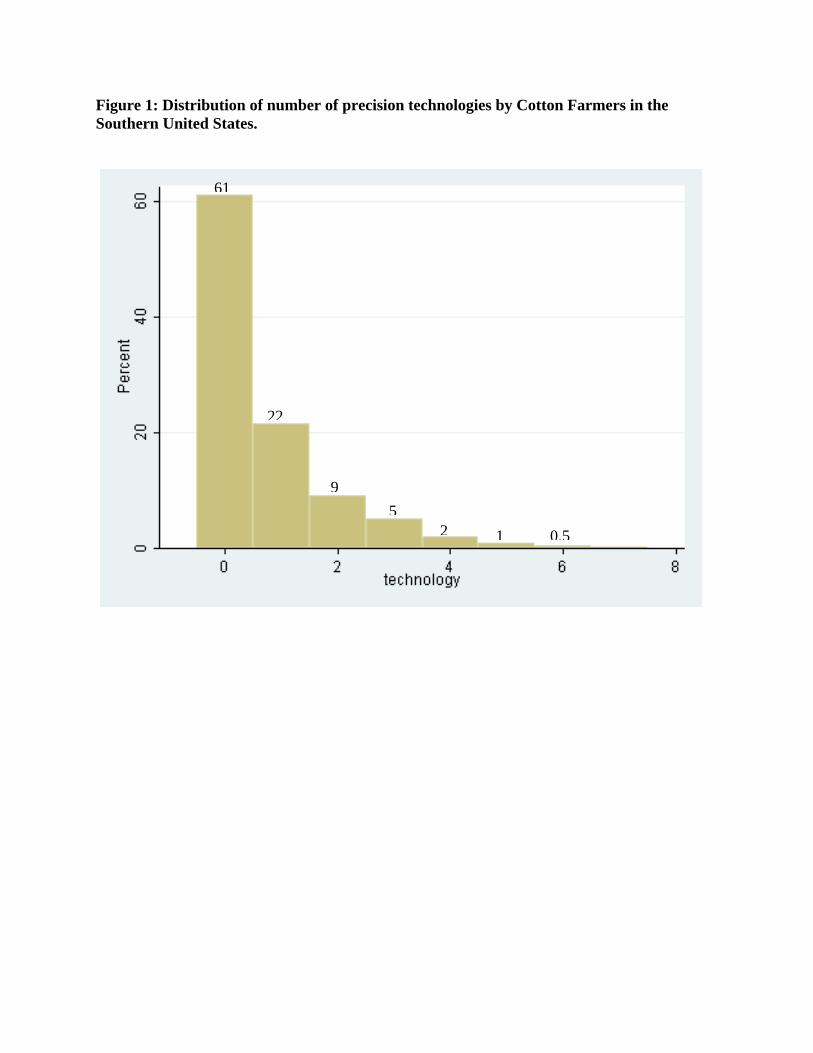
Figure 1: Distribution of number of precision technologies by Cotton Farmers in the Southern United States.

61

22

95

2 1 0.5

Table 1: Definition of variables and summary statistics Variable Definition Means

(Std. dev) NUMTECH Number of precision technology adopted 0.85

(1.204) OP_AGE Age of farm operator (years) 49.29

(11.275) F_EXPERIENCE Farming experience (years) 25.81

(11.443) OP_EDUC Formal education of farm operator (years) 14.36

(2.196) COMPFARM =1 if farmer uses computer for farm management 0.58

(0.492) SHARE_RENTED Percentage of rented acres in total operated acres 65.81

(33.772) FARMPLAN =1 if the farm operator is planning to expand size of the

operation or acquire assets to generate additional income 0.72

(0.446) FUTURE_ADOPT =1 if the farm operator thinks it would be profitable to use

precision technologies in the future 0.54

(0.498) F_INCOME Percentage of farm income in total household income 73.08

(27.814) LN_SP_YVAR Log Spatial yield variability 10.65

(1.132) S_ALABAMA Dummy variable, =1 if state is Alabama 0.12

(0.321) S_NR_CAROLINA Dummy variable, =1 if state is North Carolina 0.18

(0.383) S_FLORIDA Dummy variable, =1 if state is Florida 0.02

(0.133) S_GEORGIA Dummy variable, =1 if state is Georgia 0.18

(0.381) S_MISSISSIPPI Dummy variable, =1 if state is Mississippi 0.13

(0.339) S_LOUISIANA Dummy variable, =1 if state is Louisiana 0.07

(0.258) S_SO_CAROLINA Dummy variable, =1 if state is South Carolina 0.06

(0.238) S_MISSOURI Dummy variable, =1 if state is Missouri 0.03

(0.181) S_TENNESSEE Dummy variable, =1 if state is Tennessee 0.09

(0.280) S_VIRGINA Dummy variable, =1 if state is Virginia 0.03

(0.171) Sample 892 Source: 2005 Southern Precision Farming Survey

Table 2: Parameter estimates of factors affecting number of precision farming tools by cotton farmers in the Southern U.S.

Variable Negative Binomial Model Parameter Estimates1

Marginal effect2

Intercept -2.352*** (0.685)

--

OP_AGE -0.017** (0.008)

-0.020**

OP_EDUC 0.093*** (0.023)

0.080***

F_EXPERIENCE 0.001 (0.008)

0.001

COMPFARM 0.553*** (0.108)

0.425***

SHARE_RENTED -0.001 (0.001)

-0.001

FARMPLAN -0.233** (0.110)

-0.211**

FUTURE_ADOPT 0.530*** (0.103)

0.416***

F_INCOME 0.002** (0.001)

0.002**

LN_SPYVAR 0.078** (0.037)

0.070**

S_ALABAMA 0.078 (0.026)

0.068

S_NR_CAROLINA 0.039 (0.196)

0.034

S_FLORIDA -0.710 (0.513)

-0.437**

S_GEORGIA 0.006 (0.199)

0.006

S_MISSISSIPPI 0.509*** (0.190)

0.521***

S_LOUISIANA 0.277 (0.217)

0.266

S_SO_CAROLINA 0.344 (0.234)

0.344

S_MISSOURI 0.472* (0.269)

0.507**

S_TENNESSEE 0.103 (0.220)

0.092

S_VIRGINA 0.105 (0.309)

0.094

Wald chi Square 199.20*** Correlation between observed and predicted 70.01 Log-likelihood -970.174 Overdispersion test 33.20*** 1Numbers in parentheses are standard errors. Significance at the 10%, 5%, and 1% are indicated by single, double and triple asterisks, respectively. 2 The marginal is calculated on the sample mean. Using STATA one can obtain the effect on the conditional mean of y of a change in one of the regressors, say xj

Precision Agriculture Technology Adoption...

Documents

Transcript of Precision Agriculture Technology Adoption...