Adoption of improved citrus orchard management practices ...

PRECISION FARMING TECHNOLOGY ADOPTION
IN FLORIDA CITRUS PRODUCTION: A SURVEY AND ANALYSIS, CASE STUDY,
AND THEORETICAL REVIEW
By
BRIAN JAMES SEVIER
A DISSERTATION PRESENTED TO THE GRADUATE SCHOOL OF THE UNIVERSITY OF FLORIDA IN PARTIAL FULFILLMENT
OF THE REQUIREMENTS FOR THE DEGREE OF DOCTOR OF PHILOSOPHY
UNIVERSITY OF FLORIDA
2005

Copyright 2005
by
Brian James Sevier
This document is dedicated to my family. To my wife Danielle and son Tristan whom have endured the long hours of research and travel, data analysis and finally writing.
Danielle you have provided confidence and comfort when needed, and that little extra kick when I didn’t want to keep going!! Tristan, now that this is done we have more time
to play football in the yard and be buddies again. To Mom and Dad, who were always there to give that extra push when it was needed too. To my brother Kevin, who was
always ready to say let’s go fishing, well bro’ we finally have time to do that now.
iv
ACKNOWLEDGMENTS
I would like to acknowledge the support I have received from my graduate
committee. I have been inclined to do things “my way,” and they of course have found
ways to steer me back on track. I thank Drs. Lee, Jones, Spreen, Taylor and Schueller,
for hanging in there with me.
I would also like to acknowledge the faculty and staff of the UF/IFAS Food &
Resource Economics Department. Their support in processing surveys, developing
statistical models, and document review was unsurpassable in allowing me to finish this
dissertation and hence the degree. Special thanks go to Dr. Lisa House for endless hours
of document editing, and review and lastly thanks go to Dr. Robert Degner for making
the survey happen!

v
TABLE OF CONTENTS page
ACKNOWLEDGMENTS ................................................................................................. iv
LIST OF TABLES............................................................................................................ vii
LIST OF FIGURES ......................................................................................................... viii
ABSTRACT....................................................................................................................... ix
CHAPTER
1 INTRODUCTION ........................................................................................................1
The Florida Citrus Industry ..........................................................................................1 Overview ...............................................................................................................1
Objectives .....................................................................................................................3 Potential for Technology Adoption ..............................................................................5 Precision Agriculture ....................................................................................................6
2 TECHNOLOGY ADOPTION AND A CITRUS PRODUCER SURVEY ...............10
Objectives ...................................................................................................................10 Background.................................................................................................................10
Diffusion Theory .................................................................................................10 Technology Adoption Life Cycle ........................................................................11
Methodology...............................................................................................................15 Survey and Data Collection.................................................................................15 Sample Selection .................................................................................................15 Survey Techniques ..............................................................................................18 Questionnaire Topics...........................................................................................18
Results.........................................................................................................................20 Survey Response Rate .........................................................................................20 Survey Responses................................................................................................22
Adopted Technology Percentages ................................................................22 Responses for Non-Adoption .......................................................................23 Self-Perceived Adoption Attitude ................................................................24 Grower Demographics .................................................................................25
Discussion...................................................................................................................26 The Technology Adoption Outlook in Florida Citrus Production.......................27
vi
3 FLORIDA CITRUS GROWER TECHNOLOGY ADOPTION SURVEY – PROBIT MODEL ANAYLSIS ..................................................................................29
Objectives ...................................................................................................................29 The Probit Model Defined ..........................................................................................29
Probit Model Variables........................................................................................34 Results and Discussion ...............................................................................................35
4 GROVE XYZ – A CASE STUDY ON TECHNOLOGY ADOPTION ....................39
Introduction.................................................................................................................39 Objectives ...................................................................................................................40 Case Background ........................................................................................................40
Production Strategies Prior to Adoption..............................................................41 Business Decision Strategy.........................................................................................41
The Problem ........................................................................................................41 The Alternatives ..................................................................................................42
VRT Fertilizer Application ..........................................................................42 Irrigation and Moisture Control System.......................................................44
Adoption Decisions and Analysis...............................................................................45 What Technology Adoptions Were Made...........................................................45 The Adoption Analysis........................................................................................46
VRT Fertilizer System .................................................................................46 Irrigation Monitoring and Control System...................................................54
Discussion............................................................................................................58
5 CONCLUSIONS ........................................................................................................59
Survey Analysis and Probit Model Results ................................................................59 Case Study Analysis ...................................................................................................60 Discussion and Closing Remarks ...............................................................................61
APPENDIX
A FLORIDA CITRUS GROWER TECHNOLOGY ADOPTION SURVEY...............65
B PROBIT MODEL ANALYSIS RESULTS................................................................72
C CITRUS PRODUCING AREAS OF FLORIDA .......................................................75
LIST OF REFERENCES...................................................................................................76
BIOGRAPHICAL SKETCH .............................................................................................80
vii
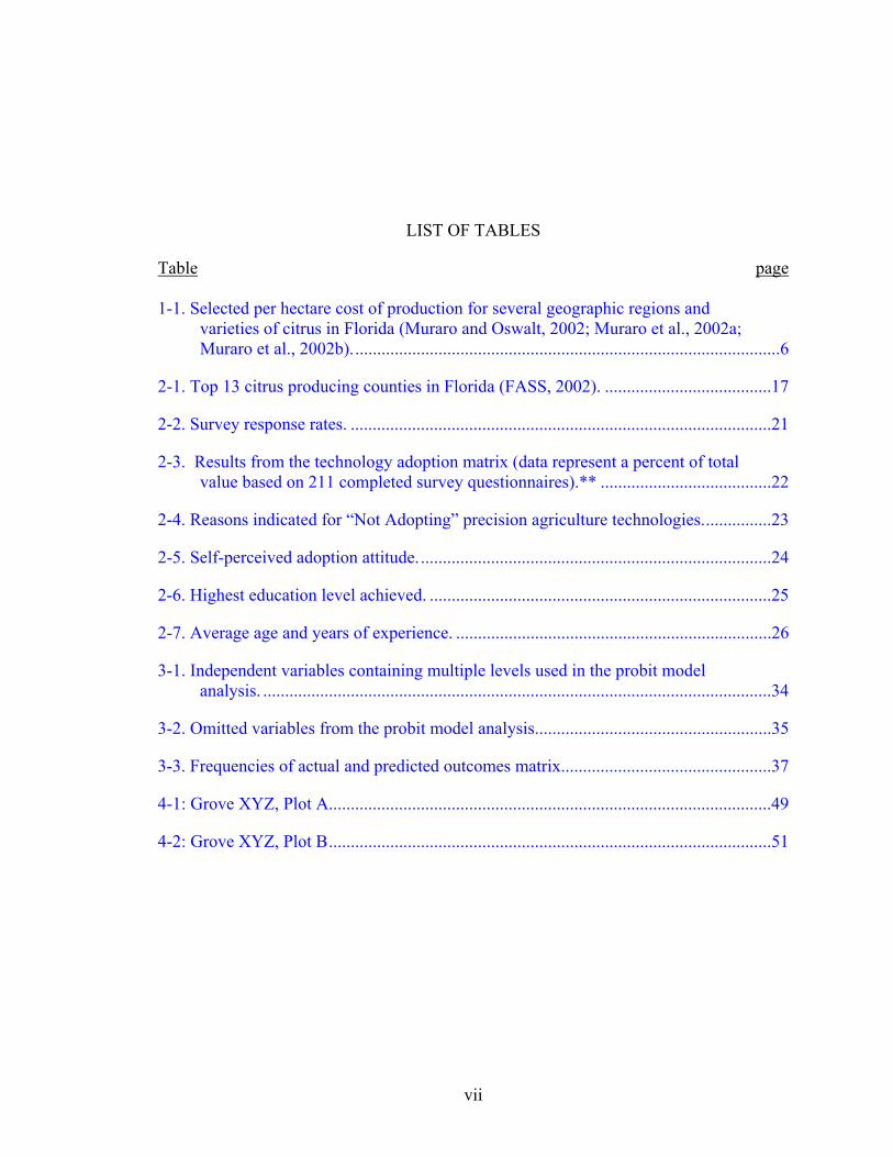
LIST OF TABLES
Table page 1-1. Selected per hectare cost of production for several geographic regions and
varieties of citrus in Florida (Muraro and Oswalt, 2002; Muraro et al., 2002a; Muraro et al., 2002b)..................................................................................................6
2-1. Top 13 citrus producing counties in Florida (FASS, 2002). ......................................17
2-2. Survey response rates. ................................................................................................21
2-3. Results from the technology adoption matrix (data represent a percent of total value based on 211 completed survey questionnaires).** .......................................22
2-4. Reasons indicated for “Not Adopting” precision agriculture technologies................23
2-5. Self-perceived adoption attitude.................................................................................24
2-6. Highest education level achieved. ..............................................................................25
2-7. Average age and years of experience. ........................................................................26
3-1. Independent variables containing multiple levels used in the probit model analysis. ....................................................................................................................34
3-2. Omitted variables from the probit model analysis......................................................35
3-3. Frequencies of actual and predicted outcomes matrix................................................37
4-1: Grove XYZ, Plot A.....................................................................................................49
4-2: Grove XYZ, Plot B.....................................................................................................51
viii
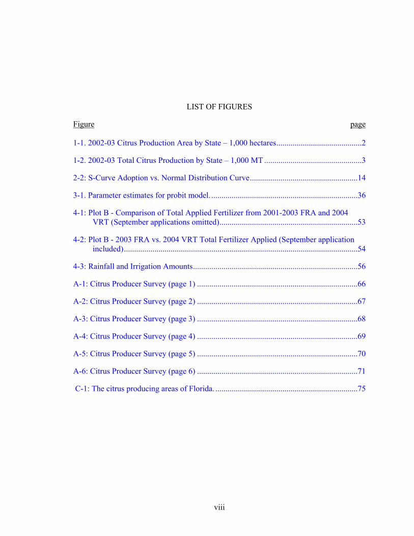
LIST OF FIGURES
Figure page 1-1. 2002-03 Citrus Production Area by State – 1,000 hectares..........................................2
1-2. 2002-03 Total Citrus Production by State – 1,000 MT ................................................3
2-2: S-Curve Adoption vs. Normal Distribution Curve.....................................................14
3-1. Parameter estimates for probit model. ........................................................................36
4-1: Plot B - Comparison of Total Applied Fertilizer from 2001-2003 FRA and 2004 VRT (September applications omitted)....................................................................53
4-2: Plot B - 2003 FRA vs. 2004 VRT Total Fertilizer Applied (September application included)...................................................................................................................54
4-3: Rainfall and Irrigation Amounts.................................................................................56
A-1: Citrus Producer Survey (page 1) ...............................................................................66
A-2: Citrus Producer Survey (page 2) ...............................................................................67
A-3: Citrus Producer Survey (page 3) ...............................................................................68
A-4: Citrus Producer Survey (page 4) ...............................................................................69
A-5: Citrus Producer Survey (page 5) ...............................................................................70
A-6: Citrus Producer Survey (page 6) ...............................................................................71
C-1: The citrus producing areas of Florida. ......................................................................75
ix
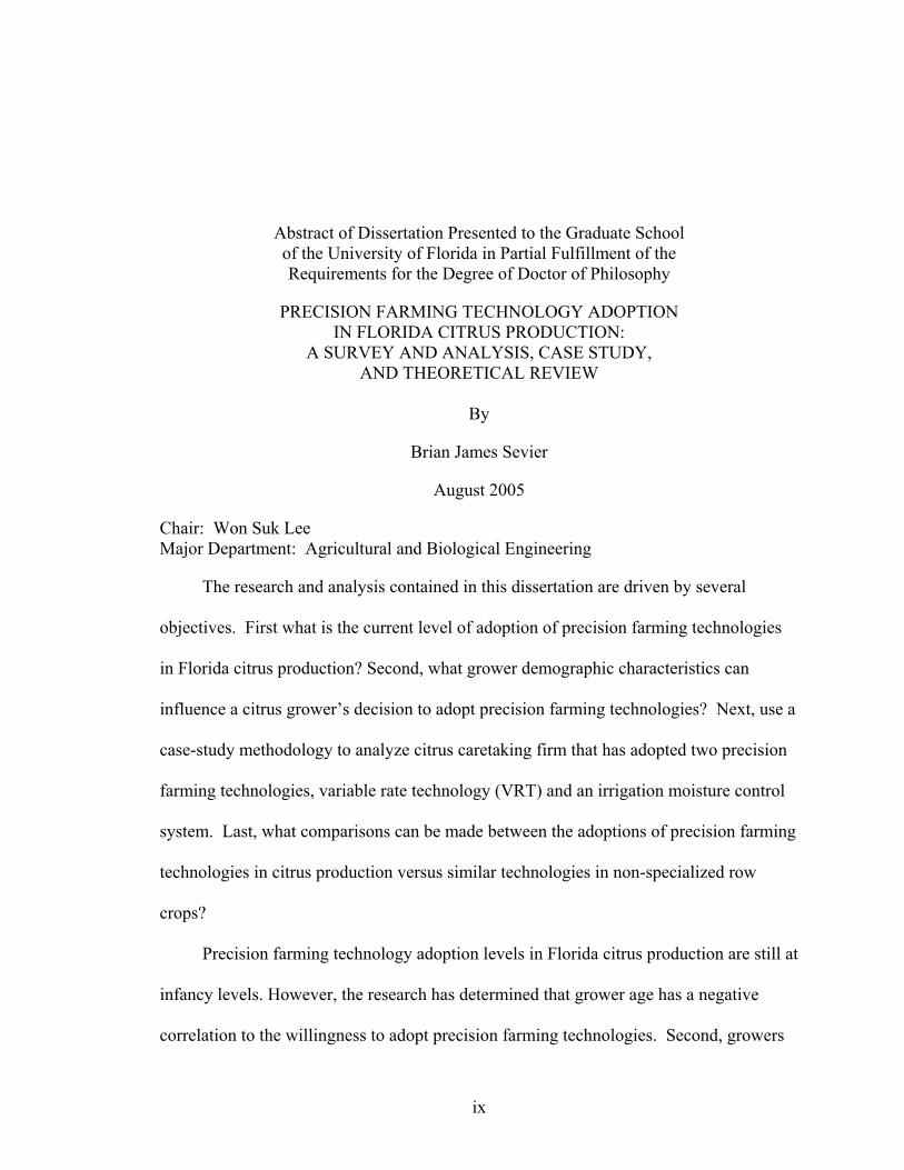
Abstract of Dissertation Presented to the Graduate School of the University of Florida in Partial Fulfillment of the Requirements for the Degree of Doctor of Philosophy
PRECISION FARMING TECHNOLOGY ADOPTION IN FLORIDA CITRUS PRODUCTION:
A SURVEY AND ANALYSIS, CASE STUDY, AND THEORETICAL REVIEW
By
Brian James Sevier
August 2005
Chair: Won Suk Lee Major Department: Agricultural and Biological Engineering
The research and analysis contained in this dissertation are driven by several
objectives. First what is the current level of adoption of precision farming technologies
in Florida citrus production? Second, what grower demographic characteristics can
influence a citrus grower’s decision to adopt precision farming technologies? Next, use a
case-study methodology to analyze citrus caretaking firm that has adopted two precision
farming technologies, variable rate technology (VRT) and an irrigation moisture control
system. Last, what comparisons can be made between the adoptions of precision farming
technologies in citrus production versus similar technologies in non-specialized row
crops?
Precision farming technology adoption levels in Florida citrus production are still at
infancy levels. However, the research has determined that grower age has a negative
correlation to the willingness to adopt precision farming technologies. Second, growers
x
managing properties with a perceived level of moderate or high in-grove spatial
variability are more likely to adopt precision farming technologies when compared to
those indicating minimal variability.
The case study analysis was performed on a citrus care taking company that has
adopted two precision farming technologies. Both the variable rate fertilizer application
and the moisture and irrigation control system have resulted in net production savings
and increased financial returns, as determined by increased marketable citrus yield.
Although still in its infancy, precision farming usage in Florida citrus faces many
barriers to adoption. The technologies in some cases are not perfected, and the buy-in by
grove owners and managers has not occurred. The potential for these precision farming
systems are existent, especially considering the pricing structure that citrus producers
operate under. They are price takers; so having the ability to decrease production costs is
one way to gain additional revenue at the margin.
1
CHAPTER 1 INTRODUCTION
The Florida Citrus Industry
Overview
Florida agriculture consists of primarily what most agriculturists consider specialty
or non-traditional crops. In the panhandle and northern end of the state, the production
area is composed primarily of soybean, peanuts, tobacco and cotton. The majority of the
production area from just north of Orlando, FL, spanning southward is dedicated to
winter vegetables and fruit, nursery and horticultural crops; and sugarcane and citrus.
Citrus was introduced to Florida between 1513 and 1563. Citrus originated in the
Orient, specifically China, and it was introduced into the New World by Christopher
Columbus via the Mediterranean. The first planting of citrus in the Americas by
Columbus was on the island of Hispaniola. Juan de Grijalva first recorded mainland
plantings in 1518 when he landed in Central America (FASS, 2003). By the year 1563,
many groves had already been established around the areas of St. Augustine and Orange
Lake in northeastern Florida. Although these groves had been established for a number
of years, commercial production did not begin until 1763. By 1890, commercial
production in Florida consumed 46,458 hectares (ha) (Jackson and Davies, 1999).
The citrus industry began to transport fruit across the Atlantic back to Great Britain
and other European countries in 1776. In the winter of 1894-1895, the citrus industry in
northern Florida experienced its first true disaster. A major freeze killed 90-95 percent of
the state’s plantings. The freeze brought the total area of citrus plantings down to 19,506
2
hectares in a single winter. Of this area, 97 percent were immature nonbearing trees. Six
more catastrophic freezes occurred between 1899 and 1962. This forced many growers
to relocate groves farther south, out of the reach of winter freezes. Much of this
relocation and expansion occurred in the 1960’s. By 1971 there were approximately
354,910 ha of citrus in Florida (Jackson and Davies, 1999).
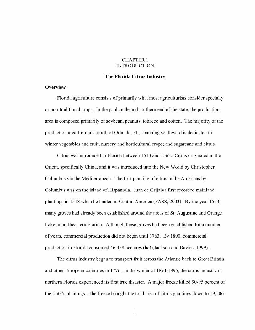
In 2002, there were 322,658 ha of citrus in commercial groves in Florida, down 4.2
percent from 2000. Bearing production area in Florida is represented in Figure 1-1 as
compared to other major citrus producing states. This figure illustrates the area in
production by state, which has mature citrus that is producing fruit for commercial sales.
Of the total production area in Florida, 81.4 percent was dedicated to orange production,
13.2 percent to grapefruit production, and the remaining 5.4 percent to specialty fruit
(e.g., tangerines, tangelos, limes, etc.) (FASS, 2002).
Texas11.0
Arizona11.0
Florida290.6
California106.3
Figure 1-1. 2002-03 Citrus Production Area by State – 1,000 hectares
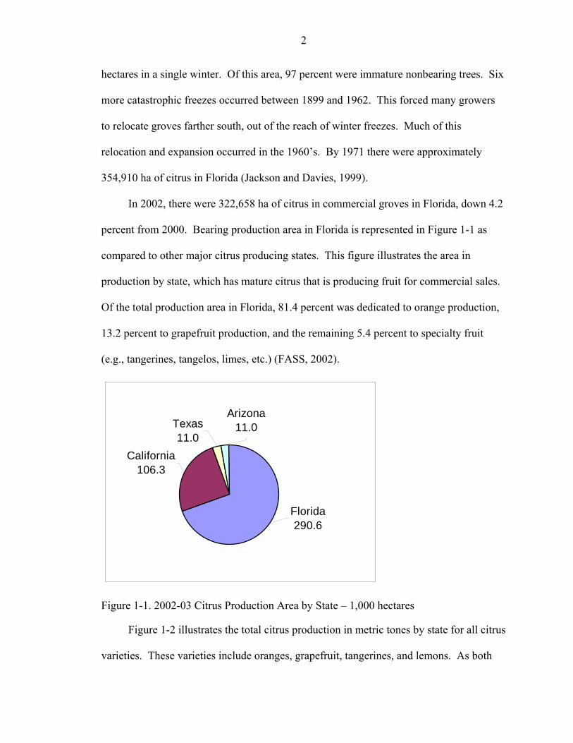
Figure 1-2 illustrates the total citrus production in metric tones by state for all citrus
varieties. These varieties include oranges, grapefruit, tangerines, and lemons. As both
3
figures reveal, Florida is the primary citrus producing state in both production area and
total production in the United States (FASS, 2003).
California3,193.3
Texas264.9
Arizona137.9
Florida10,165.9
Figure 1-2. 2002-03 Total Citrus Production by State – 1,000 MT
Objectives
There is a large amount of literature discussing the feasibility, economics, and
profitability of precision farming in agronomic crops; however there is currently no such
study on citrus. In addition, precision farming technology adoption studies have been
performed on various types of producers from many regions of the country, growing
many types of crops; again no such study has been performed on the adoption of
precision farming technologies in citrus. As illustrated in the figures above, Florida is by
far the largest producer of citrus in the United States (in both MT of yield and
commercial production area), so why wasn’t any information on the adoption of precision
farming technologies available? If the technology is available, and its effectiveness has

4
been proven in other types of cropping systems, why hadn’t Florida’s citrus producers
accepted it? Or have they?
This research study identifies the current level of adoption of precision farming
technologies in Florida citrus production, by determining “how many” growers have
adopted. Drawing from the body of literature on technology diffusion, citrus producers
will be grouped into adopter categories. These categories represent the grower’s
willingness to adopt discoveries and innovations that are presented to them. These
adopter categories assist in determining where the Florida citrus industry is in the
technology adoption life cycle, with regard to precision farming technologies.
Knowing the current level of adoption is valuable, but that only answers the
question of “how many”. The next research question that needs an answer was “who”.
In order to answer this, this study identifies grower characteristics that influence the
decision to adopt precision farming technologies. This study will also try and answer
questions like, “Does the age of the grower influence their willingness to adopt new
technologies?” or “Does the education level of the grower have an impact on their
decision to adopt site-specific crop management practices?” By answering “who”, a
demographic profile can be created for adopters of precision technologies in Florida
citrus.
In an effort to expound on “how many” and “who”, the next objective is to
determine “why”. What is the driving force that causes a citrus producer to adopt a new
technology and change their management practices? What considerations should the
grower or the firm make before deciding to invest in new technologies? These are
questions that can only be answered by a grower that has already made the adoption
5
decision. A case study analysis will be used to investigate the technology adoption
process imposed by a citrus care taking firm. By using a real company for the case study
analysis, not only can the “why” be answered, but also “what” technologies were
adopted.
Potential for Technology Adoption
There is a large potential for the adoption of precision technologies in citrus
production. Per unit costs of production of Florida citrus have been volatile, causing
producers to attempt to find ways to control this volatility. The premise behind site-
specific crop management (SSCM) technologies seems to lend itself perfectly to the
production scenario in citrus. If growers were able to manage their input applications
based on a site-specific basis, then the cost of production has the potential to be
maintained at a lower level. These inputs include herbicide, insecticide, nematicide,
fungicide, fertilization, post-bloom sprays, and irrigation. In addition there are also tree
maintenance issues with resets (newly planted nursery trees where mature trees have been
removed), topping and hedging, and chemical or mechanical mowing (Muraro and
Oswalt, 2002). If the grower is using mechanical harvesting, then chemical abscission
agents are also required to assist in removing mature fruit from trees.
Table 1-1 below, shows the annual cost of production per hectare for several types
of citrus. These figures represent the cost of production per hectare, and the percent
change from one season to the next. In all four citrus types provided in Table 1-1, the
cost of production during the 2001/02 season represents a net increase in production costs
from the 1997/98 season. Several studies have shown that the adoption of precision
agriculture technologies and practices would be biased towards crops or commodities that
are input intensive (Daberkow, 1997).

6
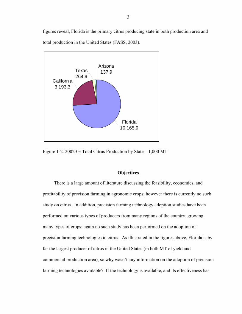
Table 1-1. Selected per hectare cost of production for several geographic regions and varieties of citrus in Florida (Muraro and Oswalt, 2002; Muraro et al., 2002a; Muraro et al., 2002b).
Indian River - Fresh White Grapefruit 97-98 98-99 99-00 00-01 01-02 per hectare cost of production $2,288.61 $2,279.67 $2,351.13 $2,407.94 $2,492.72 %change from previous season -0.39 % 3.13 % 2.42 % 3.52 %
Southwest - Processed Hamlin Oranges 97-98 98-99 99-00 00-01 01-02 per hectare cost of production $1,804.98 $1,841.38 $1,875.18 $1,900.34 $1,895.86 %change from previous season 2.02 % 1.84 % 1.34 % -0.24 %
Southwest - Fresh Red Seedless Grapefruit 97-98 98-99 99-00 00-01 01-02 per hectare cost of production $2,024.88 $2,085.49 $2,142.55 $2,136.94 $2,161.03 %change from previous season 2.99 % 2.74 % -0.26 % 1.13 %
Ridge - Processed Valencia Oranges 97-98 98-99 99-00 00-01 01-02 per hectare cost of production $1,891.98 $1,904.66 $1,935.89 $1,875.16 $1,897.20 %change from previous season 0.67 % 1.64 % -3.14 % 1.18 %
--primary data have been converted from acres to hectares
Precision Agriculture
Production practices in agriculture are constantly changing. The introduction of
site-specific crop management (SSCM), also known as precision farming, is among the
newest advances in production agriculture and mechanization. The use of multiple
technologies with traditional production practices has opened a new era of “high-tech”
farming. The use of yield monitoring, variable-rate technology (VRT) applications of
herbicide, pesticide and fertilizer, remote sensing, and soil sampling, are examples of
precision agriculture. In addition, the application of the Global Positioning System
(GPS) and geographic information systems (GIS) are major components of many
precision farming technologies. The National Research Council (NRC, 1997) defines
precision agriculture as “a management strategy that uses information technologies to
bring data from multiple sources to bear on decisions associated with crop production.”
Morgan and Ess (2003) provided the following definition for precision agriculture
“managing each crop production input…on a site-specific basis to reduce waste,
increase profits, and maintain the quality of the environment.”
7
The usefulness of precision agriculture or SSCM lies in the value of the
information. The adoption of a precision farming technology comes at a cost, and often a
high one. The efficiencies gained in production methods must outweigh the cost of
adoption, or it is economically infeasible. Precision farming technologies provide
information that is gathered from a series of interrelated components. As mentioned
above, grid sampling and yield monitoring in conjunction with GPS technologies offer a
bird’s-eye view of the production area; the grove in this study. This information is then
used to determine the spatial variability within the grove. The variability of soil
conditions, weed and pest outbreaks, and yield are then transferred into the use of
variable rate technologies to target that variability, and manage crop inputs on a site-
specific basis (Khanna et al., 2000).
Precision agriculture technologies are currently being used in the production of
cereal and grain crops; cotton, peanuts and soybean; potatoes, tomatoes, and sugar beets;
forage and grass crops; sugarcane and citrus. SSCM offers the producer an alternative to
enhancing input efficiencies over standardized production methods. These alternatives
are provided by the acquisition of information, at a cost, about spatial variability within
the production area, and then using that information to target those inputs at the locations
of the variability (Khanna et al., 2000). The purpose of precision agriculture is multifold.
First, growers seek to increase profits by maximizing yield, while simultaneously
decreasing production costs by carefully tailoring soil and crop management. Second,
producers are becoming more environmentally aware, and as a result of tailoring inputs,
more environmentally friendly practices are implemented. Potentially growers can
realize economic benefits by reducing their overall cost of production, likewise the

8
environment benefits, and what appears to be a win-win situation is a result of simply
being able to manage inputs site-specifically to production.
Daberkow and McBride (1998) in a survey study of farmers showed a low rate of
adoption of precision farming technologies. This is in spite of the potential economic and
environmental benefits. According to their results, by 1996, only 4 percent of farmers
across the US had adopted variable rate technologies, and only 6 percent had adopted
yield monitoring systems. A follow-up to the Daberkow and McBride study done in the
Midwest identified adoption levels of 12 percent on VRT systems and 10 percent on yield
monitoring (Khanna et al., 1999). The study went on to state that a number of these
“adoptions” were producers who contracted services through custom hiring instead of
purchasing the technologies outright. Farmers surveyed in their study indicated that the
reason for non-adoption included uncertainty about the payback on the high cost
investment. Last, their study indicated that farmers were intending and willing to wait on
the adoption decision, and that the adoption rates of these technologies are likely to
increase fourfold at the end of five years. The processes involved in technology diffusion
and adoption will be discussed in further detail in Chapter 2.
The following chapters of this research study will investigate the current level of
adoption of precision farming technologies in Florida citrus production. Second, the
study will investigate the demographic characteristics and variables that determine the
willingness to invest in these technologies. In an effort to expound upon the “who” and
“how many” have adopted, a case study analysis will look at the “why”, “what” and
“how” a citrus farm made the adoption decision. The research questions posed above

9
will try and determine what the current status is for precision farming in the Florida citrus
industry, and what to expect with precision farming technologies in the future.
10
CHAPTER 2 TECHNOLOGY ADOPTION AND A CITRUS PRODUCER SURVEY
Objectives
This chapter of the study is going to discuss the technology adoption life cycle as
well as the body of literature dedicated to the diffusion theory of new technologies and
innovations. In addition, this chapter will address identifying the current level of
adoption of precision farming technologies for citrus producers in the 10 largest citrus
producing counties in the state of Florida. Additionally this chapter investigates the
attitudes of adopters versus non-adopters towards technology in general. The specific
objectives for this chapter are to quantify the adoption rate of precision farming
technologies in Florida citrus production, and to determine where the industry is on the
technology life-cycle curve.
Background
Diffusion Theory
Diffusion theory is the body of work that describes the process by which
technological advances are discovered then distributed. Classical literature on the theory
of diffusion field dates back to Rogers (1962; 2003), Ruttan (1959), and Katz (1961), as
well as others even earlier. Rogers identifies four elements of the diffusion of
innovations. The first element is the “innovation” itself; the discovery of an idea,
technology, or social movement. Element two is the process by which the innovation
spreads or disseminates, hence “diffusion”. The third element is the “social system”; the
collective body or population that is encountered by this innovation. The members of the
11
social system can be individuals, firms or collective groups of either. The last element is
“time”. The diffusion of an innovation has temporal aspects that must be considered.
The innovation must travel a process of diffusion through some social system, and it must
travel the process over a period of time. Diffusion is not instantaneous and can occur
within the population by different channels of communication of the innovation (Grubler,
1998). Rogers describes the adoption process as a “…mental process through which an
individual passes from first hearing about an innovation to final adoption.” This
definition implies the affect of time on the diffusion of innovations. Geroski (2000) also
states that the diffusion process can occur rapidly, but inherently more time is spent on
the adoption of the innovation.
The diffusion of innovation is a topic that is studied by a wide variety of
disciplines. Most often economics and sociology are the fields that provide the most
attention to the subject (Fisher et al., 2000). The diffusion of innovation and the adoption
decision process, although linked, are separate and distinct processes. Diffusion is
differentiated from adoption, in that diffusion is the process by which a new product is
distributed amongst the population; adoption is the internal decision making process that
an individual or firm must go through. Many researchers, especially in the field of
economics, use binomial models to investigate technology adoption. An example of one
of the binomial models is found in Chapter 3 of this study. The life cycle of adoption and
the adoption process will be discussed in the next section of this chapter.
Technology Adoption Life Cycle
The technology adoption life cycle refers to cycle and process that an innovation
travels through to the point of adoption by some population. The population can be
12
individuals or firms; this study’s emphasis was on the adoption life cycle of precision
farming technologies and their acceptance within the Florida citrus industry.
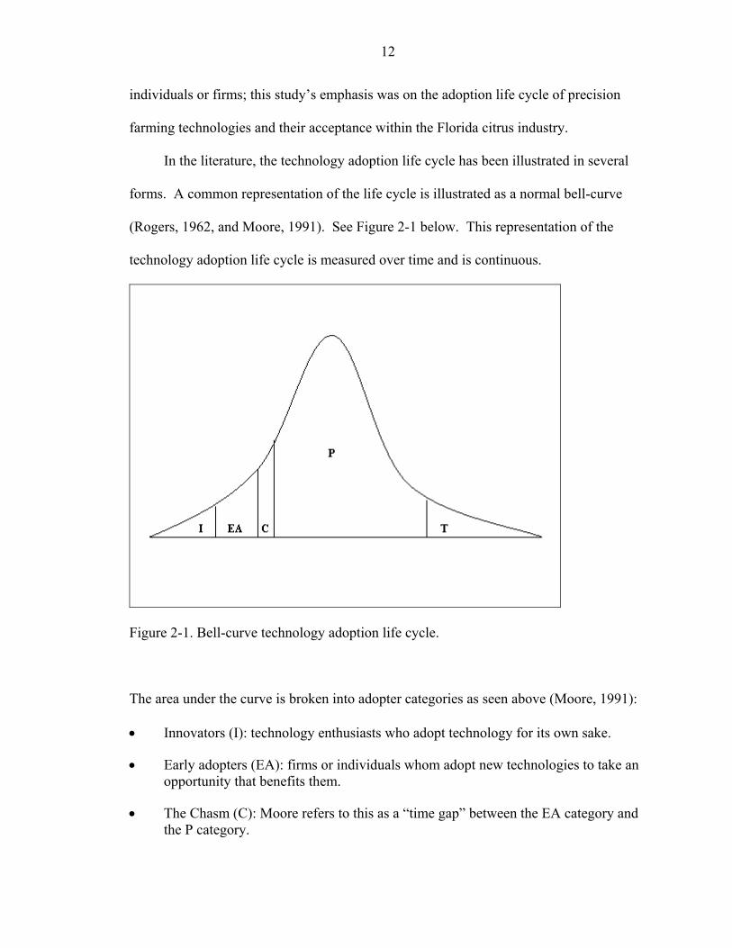
In the literature, the technology adoption life cycle has been illustrated in several
forms. A common representation of the life cycle is illustrated as a normal bell-curve
(Rogers, 1962, and Moore, 1991). See Figure 2-1 below. This representation of the
technology adoption life cycle is measured over time and is continuous.
Figure 2-1. Bell-curve technology adoption life cycle.
The area under the curve is broken into adopter categories as seen above (Moore, 1991):
• Innovators (I): technology enthusiasts who adopt technology for its own sake.
• Early adopters (EA): firms or individuals whom adopt new technologies to take an opportunity that benefits them.
• The Chasm (C): Moore refers to this as a “time gap” between the EA category and the P category.
13
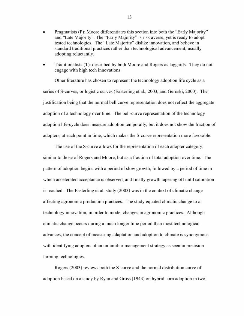
• Pragmatists (P): Moore differentiates this section into both the “Early Majority” and “Late Majority”. The “Early Majority” is risk averse, yet is ready to adopt tested technologies. The “Late Majority” dislike innovation, and believe in standard traditional practices rather than technological advancement; usually adopting reluctantly.
• Traditionalists (T): described by both Moore and Rogers as laggards. They do not engage with high tech innovations.
Other literature has chosen to represent the technology adoption life cycle as a
series of S-curves, or logistic curves (Easterling et al., 2003, and Geroski, 2000). The
justification being that the normal bell curve representation does not reflect the aggregate
adoption of a technology over time. The bell-curve representation of the technology
adoption life-cycle does measure adoption temporally, but it does not show the fraction of
adopters, at each point in time, which makes the S-curve representation more favorable.
The use of the S-curve allows for the representation of each adopter category,
similar to those of Rogers and Moore, but as a fraction of total adoption over time. The
pattern of adoption begins with a period of slow growth, followed by a period of time in
which accelerated acceptance is observed, and finally growth tapering off until saturation
is reached. The Easterling et al. study (2003) was in the context of climatic change
affecting agronomic production practices. The study equated climatic change to a
technology innovation, in order to model changes in agronomic practices. Although
climatic change occurs during a much longer time period than most technological
advances, the concept of measuring adaptation and adoption to climate is synonymous
with identifying adopters of an unfamiliar management strategy as seen in precision
farming technologies.
Rogers (2003) reviews both the S-curve and the normal distribution curve of
adoption based on a study by Ryan and Gross (1943) on hybrid corn adoption in two
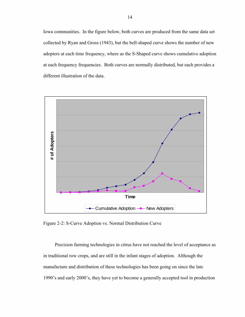
14
Iowa communities. In the figure below, both curves are produced from the same data set
collected by Ryan and Gross (1943), but the bell-shaped curve shows the number of new
adopters at each time frequency, where as the S-Shaped curve shows cumulative adoption
at each frequency frequencies. Both curves are normally distributed, but each provides a
different illustration of the data.
Time
# of
Ado
pter
s
Cumulative Adoption New Adopters
Figure 2-2: S-Curve Adoption vs. Normal Distribution Curve
Precision farming technologies in citrus have not reached the level of acceptance as
in traditional row crops, and are still in the infant stages of adoption. Although the
manufacture and distribution of these technologies has been going on since the late
1990’s and early 2000’s, they have yet to become a generally accepted tool in production

15
management. These site-specific technologies are still undergoing rapid improvements,
causing many early adopters to feel “penalized”. As witnessed in the information
technology industry, obsolescence occurs very rapidly. Early adopters are willing to be
the first to buy-in; yet they have undoubtedly paid a premium for technology that will
still undergo many evolutions of technological change and perfection. In addition,
current prices for these technologies will decrease as demand grows; allowing
manufacturers allocate more economies of scale to their production (Khanna et al, 2000).
Early adopters essentially forfeit their ability to invest in the “new and improved” next
generation of their adopted technology, at least not until their original investment has
been fully depreciated.
Methodology
Survey and Data Collection
The primary instrument used to carry out this research to determine the current
technology adoption levels was a mail survey questionnaire. The self-administered
questionnaire is an efficient and cost-effective way to collect data from a large and often
geographically disbursed group (Fowler, 2002). The first step in any survey-based
research is to identify a sample, and then a sample frame. The population of interest is
citrus producers in the state of Florida.
Sample Selection
In previous research (D’Souza et al., 1993; Daberkow and McBride, 1998; Khanna,
2001), it was determined that one of the primary barriers to adoption of alternative
production practices was the scale of the operation. In citrus production, scale can be
defined in two ways. First, scale can simply be the production area (acres or hectares) of
planted commercial citrus. Second, scale can be stated in the number of trees (total area

16
multiplied by the tree density). Tree density (trees planted per ha), is not a static variable
in the Florida citrus industry, so it is difficult to determine tree counts accurately. For
example, in the early 1970’s, average tree density for oranges and grapefruits was
approximately 198 trees per ha and 180 trees per ha, respectively. As of 2002, tree
density was approximately 326 trees per ha for citrus and 267 trees per ha for grapefruit
(FASS, 2002). Since tree density can vary so greatly, the scale was determined to be the
production area of planted commercial citrus in hectares.
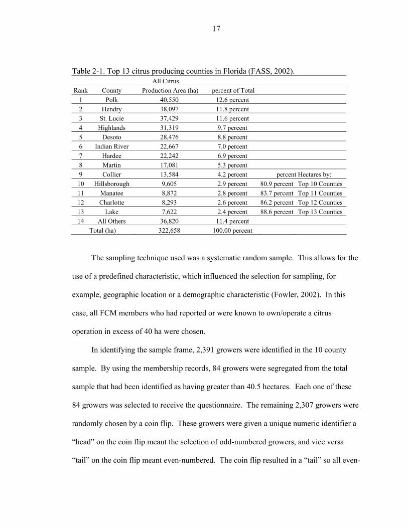
In identifying a sample, the top 10 citrus producing counties in the state were
selected based on area in citrus production. Table 2-1 itemizes each county and its
respective percentage of the total citrus production area in the state. Counties eleven
through thirteen counties were omitted from the survey sample due to the nature of the
ownership in those counties. In Lake County alone, there was an estimated 2,000
growers with relatively small groves (fewer than 4 ha per owner). This clientele would
inherently be the last group expected to adopt precision technologies based on the
assumption of scale as a barrier. A map of the geographic areas that were sampled is
provided in Appendix C.
By assuming scale to be a barrier to adoption, the focus was on growers who had
been identified in the industry as having at least 40 ha of area dedicated to citrus
production. The state’s main growers association, Florida Citrus Mutual (FCM),
provided information on growers’ scales of operation. By using FCM membership
records, small growers were segregated from large growers.
17
Table 2-1. Top 13 citrus producing counties in Florida (FASS, 2002). All Citrus
Rank County Production Area (ha) percent of Total 1 Polk 40,550 12.6 percent 2 Hendry 38,097 11.8 percent 3 St. Lucie 37,429 11.6 percent 4 Highlands 31,319 9.7 percent 5 Desoto 28,476 8.8 percent 6 Indian River 22,667 7.0 percent 7 Hardee 22,242 6.9 percent 8 Martin 17,081 5.3 percent 9 Collier 13,584 4.2 percent percent Hectares by:
10 Hillsborough 9,605 2.9 percent 80.9 percent Top 10 Counties 11 Manatee 8,872 2.8 percent 83.7 percent Top 11 Counties 12 Charlotte 8,293 2.6 percent 86.2 percent Top 12 Counties 13 Lake 7,622 2.4 percent 88.6 percent Top 13 Counties 14 All Others 36,820 11.4 percent
Total (ha) 322,658 100.00 percent
The sampling technique used was a systematic random sample. This allows for the
use of a predefined characteristic, which influenced the selection for sampling, for
example, geographic location or a demographic characteristic (Fowler, 2002). In this
case, all FCM members who had reported or were known to own/operate a citrus
operation in excess of 40 ha were chosen.
In identifying the sample frame, 2,391 growers were identified in the 10 county
sample. By using the membership records, 84 growers were segregated from the total
sample that had been identified as having greater than 40.5 hectares. Each one of these
84 growers was selected to receive the questionnaire. The remaining 2,307 growers were
randomly chosen by a coin flip. These growers were given a unique numeric identifier a
“head” on the coin flip meant the selection of odd-numbered growers, and vice versa
“tail” on the coin flip meant even-numbered. The coin flip resulted in a “tail” so all even-

18
numbered growers were then selected to receive the questionnaire. The final sample
frame was narrowed down to all of the 84 “large” growers and the remaining even-
numbered growers. This resulted in a mail survey of 1,232 growers. The use of
production area as a segregation tool and then following with a coin flip to randomize the
remaining sample resulted in what is referred to as a “systematic random sample”
(Fowler, 2002). The sample frame resulted in selecting more than 50 percent of the
member growers available in the 10 county sample.
Survey Techniques
After the randomization exercise, a unique numeric identifier was assigned to each
of the survey participants; this is a common market-research practice in order to track
respondent participation. This numeric identifier was affixed as a control number using a
self-adhesive label to all correspondence going to the respective participants. As
responses were received, the identifier was used not for data association, but simply to
remove the participant from future mailings.
Using a mail survey methodology established by D. A. Dillman (Fowler, 2002),
selected participants received a questionnaire in the mail in late March 2003. A reminder
card was sent to all of the non-respondents within 7-10 days in early April 2003. Last,
another 7-10 days after the reminder card was sent, a complete second packet was also
sent in an attempt to collect a response. Survey questionnaires were accepted for
approximately six months.
Questionnaire Topics
The primary research question was to identify the rate of technology adoption in
Florida citrus production. In order to determine this adoption rate, a response matrix was
provided to the participants (the survey instrument is included in Appendix A). The
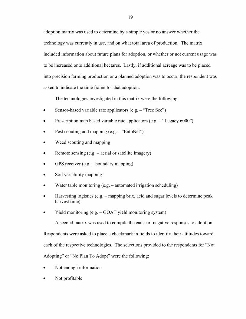
19
adoption matrix was used to determine by a simple yes or no answer whether the
technology was currently in use, and on what total area of production. The matrix
included information about future plans for adoption, or whether or not current usage was
to be increased onto additional hectares. Lastly, if additional acreage was to be placed
into precision farming production or a planned adoption was to occur, the respondent was
asked to indicate the time frame for that adoption.
The technologies investigated in this matrix were the following:
• Sensor-based variable rate applicators (e.g. – “Tree See”)
• Prescription map based variable rate applicators (e.g. – “Legacy 6000”)
• Pest scouting and mapping (e.g. – “EntoNet”)
• Weed scouting and mapping
• Remote sensing (e.g. – aerial or satellite imagery)
• GPS receiver (e.g. – boundary mapping)
• Soil variability mapping
• Water table monitoring (e.g. – automated irrigation scheduling)
• Harvesting logistics (e.g. – mapping brix, acid and sugar levels to determine peak harvest time)
• Yield monitoring (e.g. – GOAT yield monitoring system)
A second matrix was used to compile the cause of negative responses to adoption.
Respondents were asked to place a checkmark in fields to identify their attitudes toward
each of the respective technologies. The selections provided to the respondents for “Not
Adopting” or “No Plan To Adopt” were the following:
• Not enough information
• Not profitable

20
• Lack of capital
• Process/equipment not reliable
• Process/equipment too complex for laborers
• Satisfied with current practices
• Other (please specify)
Additional information was collected for the purpose of establishing demographic
profiles for adopters versus non-adopters. These questions also provided information
pertaining to the cost of production estimates for these growers for future research in
connection with the profile that is built.
These questions included the following:
• Grower demographic information (age, highest education level achieved, and grove management experience)
• Size and type of operation (hectares of fresh oranges or grapefruit, processed oranges or grapefruit, or “other” citrus)
• Counties and Water Management Districts of operation
• Types of irrigation used
• Rootstocks of respective citrus varieties as well as average age of the grove
• Personal willingness to adopt technology
• Current use of computer applications (email, internet, financial record keeping, weather networks, GIS, expert decision systems for production management, or none)
• Ability to identify the current level of in-grove variability
Results
Survey Response Rate
The analysis of the response rates followed guidelines discussed by Fowler (2002).
The raw response rate was simply the number of returned questionnaires as a percent of
21
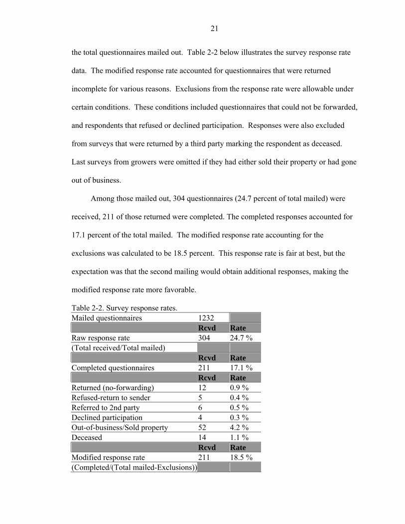
the total questionnaires mailed out. Table 2-2 below illustrates the survey response rate
data. The modified response rate accounted for questionnaires that were returned
incomplete for various reasons. Exclusions from the response rate were allowable under
certain conditions. These conditions included questionnaires that could not be forwarded,
and respondents that refused or declined participation. Responses were also excluded
from surveys that were returned by a third party marking the respondent as deceased.
Last surveys from growers were omitted if they had either sold their property or had gone
out of business.
Among those mailed out, 304 questionnaires (24.7 percent of total mailed) were
received, 211 of those returned were completed. The completed responses accounted for
17.1 percent of the total mailed. The modified response rate accounting for the
exclusions was calculated to be 18.5 percent. This response rate is fair at best, but the
expectation was that the second mailing would obtain additional responses, making the
modified response rate more favorable.
Table 2-2. Survey response rates. Mailed questionnaires 1232 Rcvd Rate Raw response rate 304 24.7 % (Total received/Total mailed) Rcvd Rate Completed questionnaires 211 17.1 % Rcvd Rate Returned (no-forwarding) 12 0.9 % Refused-return to sender 5 0.4 % Referred to 2nd party 6 0.5 % Declined participation 4 0.3 % Out-of-business/Sold property 52 4.2 % Deceased 14 1.1 % Rcvd Rate Modified response rate 211 18.5 % (Completed/(Total mailed-Exclusions))
22
Survey Responses
Adopted Technology Percentages
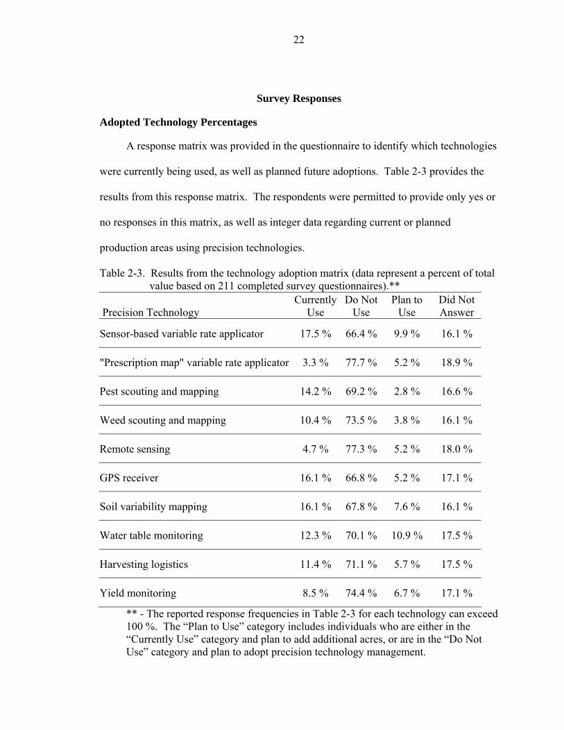
A response matrix was provided in the questionnaire to identify which technologies
were currently being used, as well as planned future adoptions. Table 2-3 provides the
results from this response matrix. The respondents were permitted to provide only yes or
no responses in this matrix, as well as integer data regarding current or planned
production areas using precision technologies.
Table 2-3. Results from the technology adoption matrix (data represent a percent of total value based on 211 completed survey questionnaires).**
Precision Technology Currently
Use Do Not
Use Plan to
Use Did Not Answer
Sensor-based variable rate applicator 17.5 % 66.4 % 9.9 % 16.1 %
"Prescription map" variable rate applicator 3.3 % 77.7 % 5.2 % 18.9 %
Pest scouting and mapping 14.2 % 69.2 % 2.8 % 16.6 %
Weed scouting and mapping 10.4 % 73.5 % 3.8 % 16.1 %
Remote sensing 4.7 % 77.3 % 5.2 % 18.0 %
GPS receiver 16.1 % 66.8 % 5.2 % 17.1 %
Soil variability mapping 16.1 % 67.8 % 7.6 % 16.1 %
Water table monitoring 12.3 % 70.1 % 10.9 % 17.5 %
Harvesting logistics 11.4 % 71.1 % 5.7 % 17.5 %
Yield monitoring 8.5 % 74.4 % 6.7 % 17.1 %
** - The reported response frequencies in Table 2-3 for each technology can exceed 100 %. The “Plan to Use” category includes individuals who are either in the “Currently Use” category and plan to add additional acres, or are in the “Do Not Use” category and plan to adopt precision technology management.

23
The data are presented as a percent of total from the 211 completed questionnaires.
Currently, the most commonly used precision agriculture technologies are the sensor-
based variable rate applicators (17.5 percent of the completed surveys indicated use), soil
variability mapping (16.1 percent), and GPS boundary mapping (16.1 percent). The least
commonly used technologies are remote sensing (e.g., aerial or satellite imagery) with its
current level of adoption at 4.7 percent and "prescription map" variable rate controllers at
3.3 percent.
Responses for Non-Adoption
A second response matrix was used to determine reasons for “Not Adopting”
precision farming technologies. The results from this matrix can be seen in table 2-4.
The respondent was permitted to make multiple selections so the data is represented as
frequency data, not a percent of total. By far, the most common response
Table 2-4. Reasons indicated for “Not Adopting” precision agriculture technologies. Precision Technology A B C D E F
Sensor-based variable rate applicator 36 17 40 9 6 65
"Prescription map" variable rate applicator 48 16 40 8 7 68
Pest scouting and mapping 45 14 33 2 5 68
Weed scouting and mapping 39 18 33 1 1 77
Remote sensing 51 19 38 3 3 60 GPS receiver 33 17 37 1 1 64 Soil variability mapping 40 13 34 3 1 61 Water table monitoring 31 13 36 7 2 69 Harvesting logistics 42 16 33 4 2 68 Yield monitoring 48 17 35 11 7 60
A – Not Enough Information B – Not Profitable C – Lack of Capital D – Process/Equipment not Reliable E – Process/Equipment too Complex for Laborers F – Satisfied with Current Practices
24
in this matrix was that producers were satisfied with their current production practices,
for all of the investigated technologies. The next most common responses were lack of
information regarding the respective technologies, and lack of capital in order to make
the investment in new technologies.
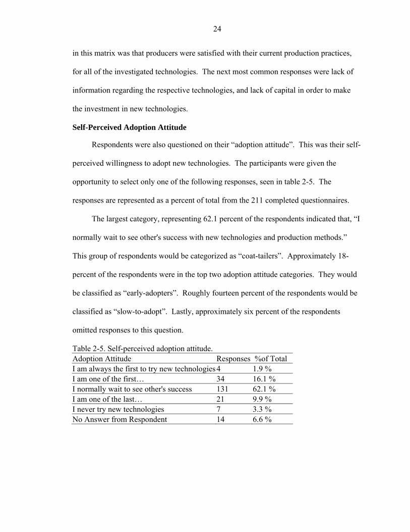
Self-Perceived Adoption Attitude
Respondents were also questioned on their “adoption attitude”. This was their self-
perceived willingness to adopt new technologies. The participants were given the
opportunity to select only one of the following responses, seen in table 2-5. The
responses are represented as a percent of total from the 211 completed questionnaires.
The largest category, representing 62.1 percent of the respondents indicated that, “I
normally wait to see other's success with new technologies and production methods.”
This group of respondents would be categorized as “coat-tailers”. Approximately 18-
percent of the respondents were in the top two adoption attitude categories. They would
be classified as “early-adopters”. Roughly fourteen percent of the respondents would be
classified as “slow-to-adopt”. Lastly, approximately six percent of the respondents
omitted responses to this question.
Table 2-5. Self-perceived adoption attitude. Adoption Attitude Responses %of Total I am always the first to try new technologies 4 1.9 % I am one of the first… 34 16.1 % I normally wait to see other's success 131 62.1 % I am one of the last… 21 9.9 % I never try new technologies 7 3.3 % No Answer from Respondent 14 6.6 %

25
Grower Demographics
The last section of the questionnaire was dedicated to the demographic profiles of
the respondents. These questions investigated the respondents’ age, years of experience
in the citrus industry, and highest level of education achieved.
The highest educational level achieved is represented as a percent of total in table
2-6. The respondent was asked to select only one maximum level. If multiple entries
were chosen, inherently the highest level was chosen during the data entry process as the
question had requested. These results are based on 211 completed questionnaires.
Approximately 81 percent of the respondents reported having had some college
education. Sixteen percent of the respondents reported a high school education or lower.
Approximately three percent of the responses were unanswered for this question.
Table 2-6. Highest education level achieved.
Education Level Responses %of Total
High school or below 34 16.1 % Some college 52 24.6 % College graduate 88 41.7 % Graduate or professional degree31 14.7 % No answer from respondent 6 2.8 %
Experience in the citrus industry was another variable analyzed to determine if it
influenced the technology adoption decision. The average reported years of experience
by the 211 respondents, was 31.4 years with a standard deviation of 15.3. The maximum
and minimum responses to this question were 85 years and 0 years of experience,
respectively. Hence there is a great deal of variability in the owners and managers of
citrus production areas, with regard to their experience in citrus production. Likewise,
the average age of the respondent was 61.1 years old with a standard deviation of 13.8.

26
The youngest respondent was 24 years old and the oldest was 92. The resulting central
tendencies for both age and years of experience are listed in table 2-7 below.
Table 2-7. Average age and years of experience. Age (yrs) Experience (yrs) Mean 61.1 31.4 Min 24 0 Max 92 85 St. Dev. 13.8 15.3
Discussion
The survey instrument was created in order to determine the current level of
adoption of precision farming technologies in Florida citrus. Based on the results from
the survey, the most commonly used precision technologies in Florida citrus production
were the sensor-based variable rate applicators and the soil variability mapping. The
least commonly used technology was remote sensing, and as indicated in open-ended
responses, this was as a result of the value of the information being far less than the cost
to acquire the information.
The most prevalent reason for not adopting new technologies was quite simply that
the respondents were satisfied with their current production practices. Anecdotally, “why
change it if it already works”.
Additionally in the survey, open-ended responses were provided for respondents to
provide additional insight as to reasons for non-adoption. Although not many growers
used this response field in the questionnaire matrix, approximately 20 respondents
indicated that the Cooperative Extension Service needed to play a larger role in
disseminating more information regarding the effectiveness and profitability of precision
farming technologies for Florida citrus producers. However, Daberkow and McBride
27
(2003) in a recent study identified that the awareness of precision agriculture
technologies has no impact on the willingness to adopt them for production management.
The Technology Adoption Outlook in Florida Citrus Production
As the survey results indicate, the adoption of precision farming technologies and
strategies have been slow at best in Florida citrus production. Research and development
by both the University of Florida and private industry continue to adapt precision farming
technologies for use in citrus production (Wei and Salyani, 2004; Annamalai and Lee,
2003; Brown, 2002; Whitney et al., 2001; Annamalai et al., 2004; Miller and Whitney,
2003; Townsend, 2004).
Citrus, being a perennial tree, is managed quite differently than the crops which
most precision farming technologies are tailored to. Although grid soil sampling and
mapping, boundary mapping using GPS technologies, and variable rate applicators using
prescription maps were conceptually easy to transition into citrus production, yield
monitoring and on-the-go sensor variable rate applicators have been slow in acceptance.
Yield monitoring, a technology that is the most widely accepted and adopted
technology in conventional row crops, has yet to be perfected in citrus. Yield monitoring
methods have been developed and tested, but primarily as a result of errors by grove
laborers the yield data has some inconsistencies (Schueller et al., 1999). The concept
established in that study should work if the issues related to grove worker operation could
be overcome.
The next step towards developing a yield monitoring system in citrus relies heavily
on the development and production of reliable mechanical harvesters. There are several
generations of mechanical harvesters in operation in Florida, but each has their own
issues before the majority of citrus producers are willing to accept them. On the other
28
hand, once the mechanical harvesting issues have been resolved, equipping these
harvesters with yield monitoring system, should overcome the grove worker issues that
Schueller et al., experienced.
29
CHAPTER 3 FLORIDA CITRUS GROWER TECHNOLOGY ADOPTION SURVEY – PROBIT
MODEL ANAYLSIS
Objectives
The survey research covered in the previous chapter simply identified the current
level of adoption of various precision farming technologies in Florida citrus production.
This section of the study will analyze the responses from the earlier survey, in order to
identify grower’s characteristics that influence the adoption of precision farming
technology. This analysis is performed by estimating a probit model to measure the
significance and correlation of the explanatory variables that influence precision farming
technology adoption.
The Probit Model Defined
Linear regression assumes that the dependent variable being tested is both
continuous and measured for all of the observations within the sample. In this survey, the
dependent variable is not continuous; instead it is a dichotomous binary variable. The
dependent variables were the 10 respective technologies, and each had 2 choices. The
choices were designed to measure current adoption and then planned adoption of the 10
technologies. Data was collected from surveys and recorded using a binary 0/1 response.
The respondent was scored a one (1) for a “yes” response to either “currently using” or
“planning to use” a technology. Alternatively, a negative response was assigned a zero
(0). Additionally, some survey respondents did not indicate a positive or negative
response; hence there is an incomplete measurement for that case. Given these
30
circumstances, linear regression is not appropriate, and an alternative means was used to
run a regression analysis on the survey data.
Linear regression models have other assumptions that are violated by the data in
this survey. Linearity is assumed, in that the dependent variable is linearly related to the
independent variables through the beta parameters. A theoretical illustration of a linear
regression model is shown in equation (1).
ikk xixi εβββ ++++= ...y 110i (1)
where - xi1, ..., xik are explanatory variables thought to influence the dependent
variable such as age, years of experience, and total production area. The
complete list of variables is provided in table 3-1
- β 0, β 1, ..., β k are parameters to be estimated
-ε i is the error term
The matrix formed by the observations on the x’s is assumed to be of full rank so
that the inverse of x'x exists. This assumption means there is no collinearity among the
explanatory variables. Homoscedastic and uncorrelated errors also require the errors to
have a constant variance and a randomly distributed error term (Greene, 1990).
In working with data that represent binary outcomes, there are several possible
methods to perform regression analysis. The linear probability model (LPM) is one of
such methods, but it also has shortcomings in dealing with heteroscedasticity and
normality. An LPM illustration can be seen in equation (2), where xi is an explanatory
variable thought to influence the dependent variable, denoted by yi ; the parameters to be
estimated β , and ε i is the error term.
iix εβ +=iy (2)
31
where - xi is the explanatory variable thought to influence the dependent variable
denoted by yi
- β is the parameter to be estimated
- ε i is the error term
Since the expected value of the dependent variable y given the independent variable
x is β x, the variance of y depends on xi, which implies that the variance of the errors
depends on x and is not constant, therefore not homoscedastic. In addition, binary values
(0/1) result in errors not being normally distributed, hence violating the normality
assumption as well. This results in the LPM not being appropriate for the analysis of this
study (Long, 1997).
The probit model is an acceptable alternative approach to analyze the binary data
collected in this study (Maddala, 1983). This model assumes that there is a response
variable of yi* with the following regression relationship seen in equation (3).
ii*i εx'y += β (3)
Normally, yi* is not observable, so a dummy variable (y) must be defined where:
y = 1 if yi* > 0
y = 0 otherwise
In the probit model, ixβ' is not defined by F(yi | xi) as traditionally seen in the linear
probability model (LPM), but instead it is defined by F(yi* | xi). From equation (3) and
the underlying dummy variable (y) we have
)'(Prob)1(Prob iii xy βε −>==
)'(1)1(Prob ii xFy β−−== (4)
where F is the cumulative density function for εi

32
The observed values for (y) are as a result of the binomial process with
probabilities given by equation (4) and can vary from trial to trial depending on the value
given by xi. This results in a likelihood function (L) of
∏∏==
−−−=10
)'(1[)'(yi
ii
yi
xFxFL ββ (5)
In equation (5) the functional form of F will depend on the assumptions made
about the distribution of errors (εi) from equation (3). In this case we assume that the
errors have a normal distribution, making this a normit or probit model. However, if the
cumulative distribution of the errors was logistic, than it would be referred to as the logit
model. In this case the probit model assumption of a normally distributed εi was applied
resulting in
∫−
∞− ⎟⎟⎠
⎞⎜⎜⎝
⎛−=−
σβ
πβ
/' 2
2exp
21)'( ix
i dttxF (6)
Scientific literature, especially within the area of econometrics, commonly
illustrates the probit model in the following form, shown in equation (7):
εβββ ++++== nn xx ...x)|1Pr(y 110 (7)
Equation (8) represents the probit model used in this study. The variable
definitions are shown in table 3-1. The dependent variable is USETECH. USETECH is
the variable name that represents the aggregation of all responses from the survey
questioning current use of precision farming technology in Florida citrus production. The
justification for aggregating the adoption of precision farming technologies is that
whether the grower uses one technology or multiple technologies, there is theoretically
only one adoption of a non-traditional production method.
33
εβββββ
ββββββ
+++++
++++++==
varmax10varmod9483726
2514exp3210)|1Pr(
xxxxx
xxxxxxy
ededed
adtadtageown (8)
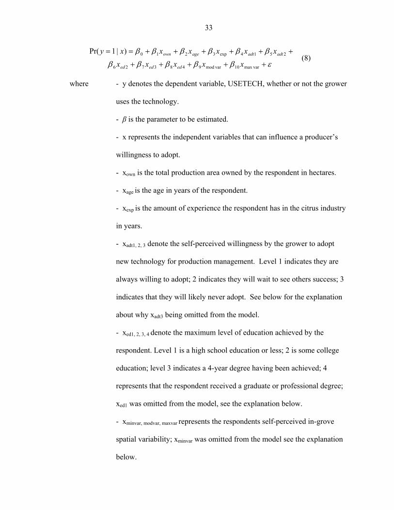
where - y denotes the dependent variable, USETECH, whether or not the grower
uses the technology.
- β is the parameter to be estimated.
- x represents the independent variables that can influence a producer’s
willingness to adopt.
- xown is the total production area owned by the respondent in hectares.
- xage is the age in years of the respondent.
- xexp is the amount of experience the respondent has in the citrus industry
in years.
- xadt1, 2, 3 denote the self-perceived willingness by the grower to adopt
new technology for production management. Level 1 indicates they are
always willing to adopt; 2 indicates they will wait to see others success; 3
indicates that they will likely never adopt. See below for the explanation
about why xadt3 being omitted from the model.
- xed1, 2, 3, 4 denote the maximum level of education achieved by the
respondent. Level 1 is a high school education or less; 2 is some college
education; level 3 indicates a 4-year degree having been achieved; 4
represents that the respondent received a graduate or professional degree;
xed1 was omitted from the model, see the explanation below.
- xminvar, modvar, maxvar represents the respondents self-perceived in-grove
spatial variability; xminvar was omitted from the model see the explanation
below.
34
- ε denotes the error term of the regression model
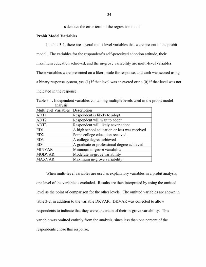
Probit Model Variables
In table 3-1, there are several multi-level variables that were present in the probit
model. The variables for the respondent’s self-perceived adoption attitude, their
maximum education achieved, and the in-grove variability are multi-level variables.
These variables were presented on a likert-scale for response, and each was scored using
a binary response system, yes (1) if that level was answered or no (0) if that level was not
indicated in the response.
Table 3-1. Independent variables containing multiple levels used in the probit model analysis.
Multilevel Variables Description ADT1 Respondent is likely to adopt ADT2 Respondent will wait to adopt ADT3 Respondent will likely never adopt ED1 A high school education or less was received ED2 Some college education received ED3 A college degree achieved ED4 A graduate or professional degree achieved MINVAR Minimum in-grove variability MODVAR Moderate in-grove variability MAXVAR Maximum in-grove variability
When multi-level variables are used as explanatory variables in a probit analysis,
one level of the variable is excluded. Results are then interpreted by using the omitted
level as the point of comparison for the other levels. The omitted variables are shown in
table 3-2, in addition to the variable DKVAR. DKVAR was collected to allow
respondents to indicate that they were uncertain of their in-grove variability. This
variable was omitted entirely from the analysis, since less than one percent of the
respondents chose this response.

35
Table 3-2. Omitted variables from the probit model analysis. Variable Name Description ADT3 Respondent never adopts ED1 A high school education or less MINVAR Minimal in-grove variability DKVAR Don’t know in-grove variability
The probit model in equation (8) was estimated using the statistical software
package LIMDEP, version 7.0 (Greene, 1995). Note that 1,232 surveys were distributed
by mail. Respondents returned more than 300 surveys, 211 were considered to be
completed and contain usable data. The estimation of the model determined that 135
observations had all of the responses completed in its entirety.
Results and Discussion
The probit model can only make estimates for responses in which every variable
measured contained a response. This being the case, the probit model could only be used
for 135 observations. The estimated model (provided in Appendix B in full detail)
indicated that three of the independent variables were statistically significant in
influencing the decision to adopt precision farming technologies, see the figure below.
The variable for the grower’s age was significant and negatively correlated to
USETECH, indicating that as the grower’s age increases, the likelihood of adopting
precision farming technologies decreased. The variables associated with the in-grove
variability resulted in two significant independent variables. The variables representing
maximum variability and moderate variability were significant and positively related to
likelihood to adopt. The positive correlation indicates that a level of variability higher
than minimum in-grove variability influenced the decision to adopt precision farming
technologies. Marginal probabilities indicate the degree to which farmers with maximum
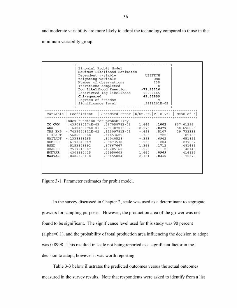
36
and moderate variability are more likely to adopt the technology compared to those in the
minimum variability group.
Figure 3-1. Parameter estimates for probit model.
In the survey discussed in Chapter 2, scale was used as a determinant to segregate
growers for sampling purposes. However, the production area of the grower was not
found to be significant. The significance level used for this study was 90 percent
(alpha=0.1), and the probability of total production area influencing the decision to adopt
was 0.8998. This resulted in scale not being reported as a significant factor in the
decision to adopt, however it was worth reporting.
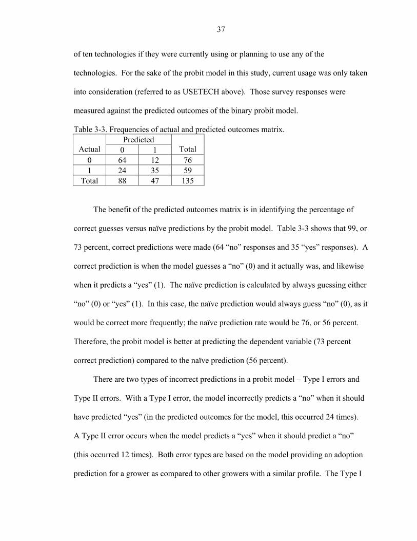
Table 3-3 below illustrates the predicted outcomes versus the actual outcomes
measured in the survey results. Note that respondents were asked to identify from a list
+---------------------------------------------+ | Binomial Probit Model | | Maximum Likelihood Estimates | | Dependent variable USETECH | | Weighting variable ONE | | Number of observations 135 | | Iterations completed 8 | | Log likelihood function -71.23216 | | Restricted log likelihood -92.50165 | | Chi-squared 42.53899 | | Degrees of freedom 9 | | Significance level .2618101E-05 | +---------------------------------------------+ +---------+--------------+----------------+--------+---------+----------+ |Variable | Coefficient | Standard Error |b/St.Er.|P[|Z|>z] | Mean of X| +---------+--------------+----------------+--------+---------+----------+ Index function for probability TC_OWN .4390390174E-03 .26705878E-03 1.644 .1002 837.61296 AGE -.1642453096E-01 .79138701E-02 -2.075 .0379 58.696296 YRS_EXP -.7439444811E-02 .11309781E-01 -.658 .5107 29.733333 LIKEADT .5686880888 .41653625 1.365 .1722 .185185 WAITADT -.1338363165 .34040528 -.393 .6942 .651851 SOMEED .6193040949 .39873538 1.553 .1204 .237037 BSED .5153843892 .37667667 1.368 .1712 .481481 GRADED .7517915387 .47205160 1.593 .1112 .148148 MODVAR .4308330425 .25950603 1.660 .0969 .414814 MAXVAR .8486323138 .39455804 2.151 .0315 .170370
37
of ten technologies if they were currently using or planning to use any of the
technologies. For the sake of the probit model in this study, current usage was only taken
into consideration (referred to as USETECH above). Those survey responses were
measured against the predicted outcomes of the binary probit model.
Table 3-3. Frequencies of actual and predicted outcomes matrix. Predicted
Actual 0 1 Total 0 64 12 76 1 24 35 59
Total 88 47 135
The benefit of the predicted outcomes matrix is in identifying the percentage of
correct guesses versus naïve predictions by the probit model. Table 3-3 shows that 99, or
73 percent, correct predictions were made (64 “no” responses and 35 “yes” responses). A
correct prediction is when the model guesses a “no” (0) and it actually was, and likewise
when it predicts a “yes” (1). The naïve prediction is calculated by always guessing either
“no” (0) or “yes” (1). In this case, the naïve prediction would always guess “no” (0), as it
would be correct more frequently; the naïve prediction rate would be 76, or 56 percent.
Therefore, the probit model is better at predicting the dependent variable (73 percent
correct prediction) compared to the naïve prediction (56 percent).
There are two types of incorrect predictions in a probit model – Type I errors and
Type II errors. With a Type I error, the model incorrectly predicts a “no” when it should
have predicted “yes” (in the predicted outcomes for the model, this occurred 24 times).
A Type II error occurs when the model predicts a “yes” when it should predict a “no”
(this occurred 12 times). Both error types are based on the model providing an adoption
prediction for a grower as compared to other growers with a similar profile. The Type I

38
error would predict the grower to “not adopt”, when actually growers of similar profiles
did adopt. Alternately, the Type II error would predict that a grower “adopt” when other
growers of a similar profile did not.
The probit model accurately predicted adoption decisions 73.3 percent of the time.
In addition, Type II error predictions only occurred 8.9 percent of the time. If this model
were to be used as a grower decision tool, more data would need to be collected in order
to validate the predictions. Although 8.9 percent is relatively low, that represents
approximately 1 in 10 incorrect predictions about whether a grower should adopt
precision farming technologies.
39
CHAPTER 4 GROVE XYZ – A CASE STUDY ON TECHNOLOGY ADOPTION
Introduction
The case study is a research strategy employed when the questions of “how” and
“why” are the goals of the investigator. Case studies are appropriate in situations where
the investigator has limited control over behavioral events and the topic focuses on a
contemporary issue versus a historical one (Yin, 2003). Case studies can assist in
answering the why question, after theoretical and statistical experimentation has
determined “what”, they do not replace these forms of experimentation, but case studies
can be used to complement them (Kennedy and Luzar, 1999). The survey discussed in
Chapter 2 of this dissertation answered the questions of “who,” “what,” “how many” and
“how much.” The goal of case study provided herein is to extend that research and to
determine the “why” related to the adoption of precision farming technologies by Grove
XYZ. Secondly, emphasis is placed on determining “how” they went about investigating
and investing in the precision technologies they chose.
Similar analyses to this case study were performed by Batte and Arnholt (2003),
where six cutting-edge farms in Ohio, who had adopted precision farming technologies.
That study used a multiple case study approach to cross-compare the six farms. Yin
(2003) indicates that the use of a single case does not decrease its validity versus multiple
case studies, as long as the single-case meets at least one of four rationales. This case fits
the third rationale that the caretaking organization at the center of this single-case or
holistic study is considered typical, or representative. The caretaking organization, other

40
than their decision to adopt precision farming technologies, is not set apart in anyway
from other caretakers. Prior to this technology adoption, their methods of managing
clients’ groves and production areas were similar to those of other caretakers who were
using traditional crop management practices without precision technologies.
Objectives
In this case study the adoption process and investment decision made by an existing
citrus caretaking organization is analyzed. Their identification has been withheld for
reasons of anonymity for their clientele. The case identifies their production practices
prior to considering the investment in precision farming technologies. In the discussion
the alternatives that were considered and the final technology adoption decision is
presented. The specific objective of this case study is to determine if the grower achieved
break even (BE) status on their investment across several precision farming technologies.
Case Background
Grove XYZ is a citrus production management company in the “Ridge” production
area of Central Florida. As a caretaker organization, their primary objective is to manage
the production, harvesting, and marketing of their clients’ citrus products. The majority
of their clients’ production capacity was targeted towards the processed orange juice
industry, however a small segment of their business, specifically tangerines, tangelos, red
grapefruit, and some oranges are sold through fresh fruit marketing channels.
The company directly controls approximately 500 hectares of citrus property that it
manages, in addition to another 1,800 hectares that it manages for its clientele. Grove
XYZ has maintained a caretaking business for fifty years. With a staff of 30 employees,
many having been with the company in excess of 15-20 years, there is quite a large

41
amount of tenure within this organization with regards to citrus production management,
and long-standing relationships with their clients.
Production Strategies Prior to Adoption
Prior to considering the adoption of precision farming technologies, XYZ followed
what most in the citrus industry consider fairly standard production practices. The grove
production manager determines, based on variety, rootstock, soil type and tree age, how
to proceed with soil amendments, tree nutrition, irrigation and necessary pesticide
applications. These production decisions were made on a grove-by-grove basis and carry
over from year to year. Production strategies change in situations of lower than expected
yield from the previous year’s harvest, future production expectations or in the case of
some weed/pest outbreak, and inclement weather such as freezes or hurricanes.
Production decisions conformed to a template that made production similar and
consistent for the entire grove, not on a site-specific basis.
Business Decision Strategy
The Problem
Grove XYZ came to a point in their organization, where the need arose to purchase
a new dry fertilizer spreader to replace a worn and obsolete spreader system. With this
purchasing decision came the opportunity to consider a variable-rate fertilizer application
spreader. Variable-rate technology (VRT) refers to the machine’s ability to vary the
applied amount of chemical while traveling through the grove. Variable-rate application
can be implemented in real-time using electronic sensors which determine tree size, or it
can be predetermined by soil sampling and then placed into a prescription map using GPS
locations to apply the predetermined rate. In this specific decision, XYZ was more
interested in considering a dry fertilizer spreader versus a VRT liquid applicator. With

42
possibly purchasing a VRT applicator, XYZ was interested in solving several production
problems:
• Resolve fertilizer application issues regarding variations in tree age.
• Realize a cost-savings by not applying a single-rate of fertilizer to immature trees in resets and also avoid applying fertilizer to skips.
• To decrease weed pressure on resets.
• Comply with Ridge Area best management practice (BMP) guidelines while still applying adequate fertilizer to high producing areas of the grove.
Secondly, XYZ was interested with better managing water resources for irrigation.
This involved both the decision to irrigate and how much irrigation to apply. Irrigation
decisions had been made by utilizing rain gauges and tensiometers located within
managed groves in conjunction with historical evapotranspiration rates, as well as
physical attributes of the trees within the grove to determine when and how much to
irrigate. In pursuing a soil monitoring system XYZ was interested in resolving the
following issues:
• Moisture monitoring for accurate irrigation scheduling.
• A tool to monitor winter stress to enhance bloom induction.
• Resolve quality concerns for fruit grown on different rootstock.
• Establish accurate measurements regarding proper irrigation management.
The Alternatives
VRT Fertilizer Application
Grove XYZ considered VRT applicators versus a standardized fixed-rate
applicator. With the use of a fixed-rate applicator, XYZ had been well aware of the
43
waste that was created by applying a single rate of materials across an entire grove. As in
many groves across the state, XYZ manages groves that contain a noticeable number of
resets or skips. Citrus trees are planted in rows, and in a mature grove that contains no
resets or skips, there are no breaks between the trees as one travels down a row with an
implement or applicator. In other words, there is a consistent string of trees in a row that
are of similar age, canopy size, tree height, and the trees have a tendency to have similar
yields from season to season.
Resets refer to a location where a tree as a result of age, disease, weather or pest
damage, or it has surpassed its optimal maturity and can no longer produce an acceptable
yield, has been replaced by a young tree. Skips refer to the location where the tree has not
been replaced and there is a “blank” spot in the row. In the scenario where a fixed-rate
applicator is being used in a grove that has a substantial number of skips or resets, the
applicator may not have the ability to stop an application where there might be a skip (no
tree at all) or a reset (a tree not needing the same application amount as a mature tree).
Hence the waste was observed by XYZ by having used a single-rate applicator in the
past.
Considering possible alternatives with regard to the VRT applicator, the decision
involved the purchase of a real-time VRT system or a prescription map-based system.
The real-time VRT system uses a system of “eyes”, and depending on the brand, this
“eye” can be based on laser, infrared or optical sensors. As the implement, in this case a
dry fertilizer spreader, travels down the rows of a grove, in “real-time” the sensors
determine the size of the next tree or even if there is a tree in the next space. If the “eye”
sees a mature tree, it applies the full amount to the location of the tree. Likewise if it sees
44
a tree of smaller size, it decreases the application amount appropriately. Lastly, if it
senses no tree at all, no material is applied to that location.
The second VRT applicator option is based on the premise of establishing a
prescription map in order to vary the rates of application. The prescription map-based
systems require the grove owner or caretaker to establish a grid sampling regime in order
to determine what materials are needed. By various methods of interpolation, a map can
be created to identify regions of variability within the grove that may need varying rates
of material. This map is then fed into a VRT applicator that is GPS controlled, and it
travels through the grove applying the prescribed rate of material to the grove based on
its location in correspondence to the prescription map.
Irrigation and Moisture Control System
The second issue that Grove XYZ needed to resolve was the irrigation and moisture
monitoring control system. XYZ began the investigation of a soil moisture sensor system
to assist with irrigation management issues. A system had recently been developed that
required the installation of soil moisture probes to monitor, log, and transmit data. These
probes measured soil capacitance to determine the moisture levels at varying depths of
the soil. The soil probes were connected to a data logger system, which was equipped
with the ability to relay data from within the grove to a centralized data storage system.
This would then allow for the grove owner or caretaker to retrieve the data pertaining to
their specific grove. Immediately XYZ recognized that not only was this going to give
them access to better data than just rainfall events and physical observation, but it was
likely going to realize a cost savings to them as well as the grove owner. For example, in
the past if a grove manager were to observe an afternoon wilt, they would have likely
irrigated. If the afternoon wilt were as a result of hot weather and excessive transpiration,

45
yet there was still sufficient moisture in the soil column, then this would have been a
false alarm and irrigation would have been applied unnecessarily. This would have
resulting wastes in pump time, pump fuel, labor requirements, and drive-time.
Admittedly, if this could be avoided the secondary benefit was that this would save water.
From a management perspective, XYZ was aware of the benefits of a system to better
inform their grove production managers in making more sound irrigation decisions.
Adoption Decisions and Analysis
What Technology Adoptions Were Made
Although XYZ was not in a position to say which VRT system was “better”, they
did feel more comfortable in determining that the real-time VRT system was a better
solution for their organization. They were more concerned with the waste associated
with materials being applied to resets and skips, where it was not needed
Grove XYZ proceeded with the decision to purchase a VRT dry fertilizer
applicator. They adopted a variable rate controller (Legacy Control System, MidTech,
Inc.) with an optic tree size sensor (CCI Eye System, Chemical Containers, Inc.). The
purchase was made in 2003 at a cost of approximately $16,000, and was placed into
production for the first fertilizer application of 2004. Since that time five (5) VRT
fertilizer applications have been made, including the January application of 2005. An
analysis on application efficiency of this adoption is presented in the following sections
of this chapter.
XYZ, with the cooperation with one of its clients, proceeded with the adoption of
an irrigation and moisture monitoring control system. The decision to purchase a soil
moisture monitoring and control system was made in April of 2003. The system is
manufactured and distributed by Agrilink Holdings Pty Ltd of Australia, and the data

46
services are maintained by AgWISE.net. The C-Probe soil moisture capacitance monitor
is manufactured and distributed by C-Probe Corporation. Both AgWISE.net and C-Probe
Corporation are subsidiaries of Agrilink International. This system was installed and
placed into operation by May of 2003, and was used to monitor soil moisture during a
“training” phase. It was placed into full production and assisting the grove manager in
irrigation scheduling and decision making in September, 2003.
The Adoption Analysis
VRT Fertilizer System
Grove XYZ provided production data from two separate groves for this portion of
the analysis. The first (Plot A) was a 70 hectare grove in the Highlands/Polk County
region of Florida. The grove is planted with early and mid varieties and Valencias. The
VRT system was implemented for two applications during the 2004 growing season from
October/2003 through September/2004. The two applications occurred on January of
2004 and March of 2004, and it was used to apply a fertilizer application. The analysis
performed and presented in Tables 4-1 and 4-2 assume that there was no change for the
costs related to equipment setup, use, time and labor. All costs were set constant to
determine the breakeven cost of the investment in the VRT spreader system.
In Table 4-1 the application data provided from XYZ is reported. In adhering to
their normal practices, for the January and March applications of 2003, the grove
manager made fertilizer recommendations of 0.44 MT/ha and 0.29 MT/ha respectively.
Having no other means to vary the application at that time, the fixed-rate applicator
applied the full amount established for that grove, on those two applications.
In 2004, the grove manager made his recommendations for the fertilizer
application, which was 0.43 MT/ha for the January fertilization. This application was
47
then made using the VRT applicator. Because the VRT system could vary the
application based on identifying resets and skips, as well as other tree age variations as
seen in the size of the tree, the full recommended application was not made. There was a
savings of 0.09 MT/ha of fertilizer applied in January 2004 from the previous year’s
January application. Likewise in 2004, there was a cost savings of approximately 20
percent from the recommended application to what was actually applied, based on the
sensor readings from the VRT. The savings of 20 percent in January 2004 related to a
cost savings of $19.94 in production costs per hectare.
In March of 2004, the grove manager’s recommendation was 0.29 MT/ha of
fertilizer. The VRT system only made an application of 0.23 MT/ha. This resulted in
0.06 MT savings of fertilizer from that same application in 2003. The savings realized
from the grove manager’s recommendation during 2004 was approximately 22 percent,
giving the grove a savings of $14.33 per hectare for fertilizer application in March of
2004.
Grove XYZ invested $15,685.00 in the MidTech Legacy Control System (with a
CCI Eye System) for their variable-rate fertilizer spreader. This investment was
scheduled for financing over seven years (or 84 months) and assumed the loan was taken
with terms of 8.00% interest per year, and loan amount equaling the full cost of the
investment. The annual financed cost of the VRT system adoption was (12 months at
$244.47/month) $2,933.64.. The cost for fertilizer was $230/MT averaged across 2003
and 2004. The average cost savings per hectare for the two fertilizer applications was
$17.14 per hectare, but XYZ was able to save a total of $34.27/ha for the entire season.
In order to recover the costs of the investment and break even (BE) on the VRT system,
48
XYZ would need to use the VRT system on 85.6 hectares to break even based on the
production costs for Plot A. This does not mean that XYZ lost money on this investment,
recall they have the ability to spread the costs of this investment over a possible 2,300 ha.
In addition, if the cost of fertilizer were to decrease to roughly $200 /MT, it would
require XYZ to implement the VRT system on approximately 98.4 ha to recover their
investment cost during that year. On the other hand if fertilizer costs were to increase to
$260 /MT, then XYZ would only need to implement its use on 75.73 ha to recover their
annual costs. The sensitivity analysis shows that the cost of adoption can be more easily
absorbed in a situation where input costs are high, because fewer hectares are required to
recover the investment cost in conjunction with higher input costs.
The analysis for Grove XYZ, Plot A assumed that this grove was the total
production area owned by a citrus producer in order to formulate the BE analysis. If this
were a grower with a production area of only 70 ha, than this grower would not have the
capacity or scale to spread the costs solely across their own production area. However,
they would have the opportunity to spread some excess capacity to other producers who
may be in a similar situation of being “too small” to afford the investment. This may be
an ideal scenario for a small to medium-sized grower to initiate a custom fertilizer service
to other small to medium-sized producers in order to breakeven on the investment.
In Table 4-2 data from another plot that is managed by XYZ is shown. This plot is
a four hectare (Plot B), planted solely in Valencias. Again for the purpose of this case
study, it is being analyzed independently from the previous plot. The data provided by
XYZ cover a four year time period. For the applications made in 2001, 2002 and 2003, a
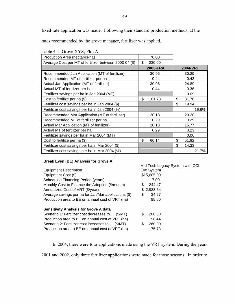
49
fixed-rate application was made. Following their standard production methods, at the
rates recommended by the grove manager, fertilizer was applied.
Table 4-1: Grove XYZ, Plot A Production Area (hectares-ha) 70.00 Average Cost per MT of fertilizer between 2003-04 ($) $ 230.00 2003-FRA 2004-VRT Recommended Jan Application (MT of fertilizer) 30.96 30.29 Recommended MT of fertilizer per ha 0.44 0.43 Actual Jan Application (MT of fertilizer) 30.96 24.89 Actual MT of fertilizer per ha 0.44 0.36 Fertilizer savings per ha in Jan 2004 (MT) 0.09 Cost to fertilize per ha ($) $ 101.73 $ 81.78 Fertilizer cost savings per ha in Jan 2004 ($) $ 19.94 Fertilizer cost savings per ha in Jan 2004 (%) 19.6%Recommended Mar Application (MT of fertilizer) 20.13 20.20 Recommended MT of fertilizer per ha 0.29 0.29 Actual Mar Application (MT of fertilizer) 20.13 15.77 Actual MT of fertilizer per ha 0.29 0.23 Fertilizer savings per ha in Mar 2004 (MT) 0.06 Cost to fertilize per ha ($) $ 66.14 $ 51.82 Fertilizer cost savings per ha in Mar 2004 ($) $ 14.33 Fertilizer cost savings per ha in Mar 2004 (%) 21.7% Break Even (BE) Analysis for Grove A
Equipment Description Mid Tech Legacy System with CCI Eye System
Equipment Cost ($) $15,685.00 Scheduled Financing Period (years) 7.00 Monthly Cost to Finance the Adoption ($/month) $ 244.47 Annualized Cost of VRT ($/year) $ 2,933.64 Average savings per ha for Jan/Mar applications ($) $ 34.27 Production area to BE on annual cost of VRT (ha) 85.60 Sensitivity Analysis for Grove A data Scenario 1: Fertilizer cost decreases to… ($/MT) $ 200.00 Production area to BE on annual cost of VRT (ha) 98.44 Scenario 2: Fertilizer cost increases to… ($/MT) $ 260.00 Production area to BE on annual cost of VRT (ha) 75.73
In 2004, there were four applications made using the VRT system. During the years
2001 and 2002, only three fertilizer applications were made for those seasons. In order to
50
properly compare VRT savings to the fixed-rate applicator, the comparison in Table 4-2
will focus on the four applications made in 2003 to the four applications made in 2004.
In January 2004, there was a savings of 0.12 MT/ha in fertilizer applied as
compared to the fertilization recommendation made by the grove manager, resulting in a
cost savings of $26.45/ha from the previous year. The applications for March and May
were quite similar, resulting in savings of 0.05 MT/ha and 0.04 MT/ha of fertilizer
applied from the 2004 recommendation, respectively. The March 2004 fertilization
saved the grower approximately $11.00/ha in production costs. Likewise, the May 2004
fertilizer application saved an additional $8.00/ha in production costs.
The final application in 2004, during September, broke away from the savings
trend as seen in the previous months. Although the application was ultimately lower than
the previous year’s application (0.89 metric tons in 2004, down from 1.06 metric tons in
2003), it was higher than the recommended application amount identified by the grove
manager. The grove manager prescribed an application of fertilizer for this grove at 0.79
MT, and the VRT system applied 0.89 MT instead, but it was still a savings of 0.04
MT/ha from the previous season’s application. The reason for this overage in application
was because the anticipated savings by the VRT system was calculated into that
application recommendation. The anticipated savings calculated by the grove manager
was not exact; however a savings was still realized. The analysis for break even was
performed on Plot B, assuming the adoption of the technology to be independent of Plot
A due to the variation in the scale of the two plots. Productions costs are spread across
the area being managed so in order to accurately reflect the cost of adoption and the
return on investment, Plot B breakeven estimates are shown in Table 4-2.

51
Table 4-2: Grove XYZ, Plot B Production Area (hectares-ha) 4.00 Average Cost per MT of fertilizer between 2003-04 ($) $ 230.00 2003-FRA 2004-VRT Recommended Jan Application (MT of fertilizer) 1.84 1.84 Recommended MT of fertilizer per ha 0.46 0.46 Actual Jan Application (MT of fertilizer) 1.84 1.38 Actual MT of fertilizer per ha 0.46 0.35 Fertilizer savings per ha in Jan 2004 (MT) 0.12 Cost to fertilize per ha ($) $ 105.80 $ 79.35 Fertilizer cost savings per ha in Jan 2004 ($) $ 26.45 Fertilizer cost savings per ha in Jan 2004 (%) 25.0%Recommended Mar Application (MT of fertilizer) 1.13 1.13 Recommended MT of fertilizer per ha 0.28 0.28 Actual Mar Application (MT of fertilizer) 1.13 0.94 Actual MT of fertilizer per ha 0.28 0.24 Fertilizer savings per ha in Mar 2004 (MT) 0.05 Cost to fertilize per ha ($) $ 64.98 $ 54.05 Fertilizer cost savings per ha in Mar 2004 ($) $ 10.93 Fertilizer cost savings per ha in Mar 2004 (%) 16.8%Recommended May Application (MT of fertilizer) 1.71 1.71 Recommended MT of fertilizer per ha 0.43 0.43 Actual Mar Application (MT of fertilzer) 1.71 1.57 Actual MT of fertilizer per ha 0.43 0.39 Fertilizer savings per ha in May 2004 (MT) 0.04 Cost to fertilize per ha ($) $ 98.33 $ 90.28 Fertilizer cost savings per ha in May 2004 ($) $ 8.05 Fertilizer cost savings per ha in May 2004 (%) 8.2%Recommended Sept Application (MT of fertilizer) 1.06 0.79 Recommended MT of fertilizer per ha 0.27 0.20 Actual Mar Application (MT of fertilzer) 1.06 0.89 Actual MT of fertilizer per ha 0.27 0.22 Fertilizer savings per ha in Sept 2004 (MT) 0.04 Cost to fertilize per ha ($) $ 60.95 $ 51.18 Fertilizer cost savings per ha in Sept 2004 ($) $ 9.78 Fertilizer cost savings per ha in Sept 2004 (%) 16.0% Break Even (BE) Analysis for Grove B
Equipment Description Mid Tech Legacy System with CCI Eye System
Equipment Cost ($) $15,685.00 Scheduled Financing Period (years) 7.00 Monthly Cost to Finance the Adoption ($/month) $ 244.47 Annualized Cost of VRT (Straight Line Depreciation) $ 2,933.64 Average savings per ha for Jan/Mar applications ($) $ 55.20 Production area to BE on annual cost of VRT (ha) 53.15
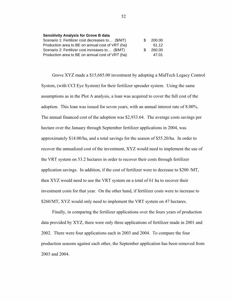
52
Sensitivity Analysis for Grove B data Scenario 1: Fertilizer cost decreases to… ($/MT) $ 200.00 Production area to BE on annual cost of VRT (ha) 61.12 Scenario 2: Fertilizer cost increases to… ($/MT) $ 260.00 Production area to BE on annual cost of VRT (ha) 47.01
Grove XYZ made a $15,685.00 investment by adopting a MidTech Legacy Control
System, (with CCI Eye System) for their fertilizer spreader system. Using the same
assumptions as in the Plot A analysis, a loan was acquired to cover the full cost of the
adoption. This loan was issued for seven years, with an annual interest rate of 8.00%.
The annual financed cost of the adoption was $2,933.64. The average costs savings per
hectare over the January through September fertilizer applications in 2004, was
approximately $14.00/ha, and a total savings for the season of $55.20/ha. In order to
recover the annualized cost of the investment, XYZ would need to implement the use of
the VRT system on 53.2 hectares in order to recover their costs through fertilizer
application savings. In addition, if the cost of fertilizer were to decrease to $200 /MT,
then XYZ would need to use the VRT system on a total of 61 ha to recover their
investment costs for that year. On the other hand, if fertilizer costs were to increase to
$260/MT, XYZ would only need to implement the VRT system on 47 hectares.
Finally, in comparing the fertilizer applications over the fours years of production
data provided by XYZ, there were only three applications of fertilizer made in 2001 and
2002. There were four applications each in 2003 and 2004. To compare the four
production seasons against each other, the September application has been removed from
2003 and 2004.

53
As shown in Figure 4-1, for the January through May fertilizer applications over
the four years, there were similar recommendations and applications made in 2001 and
2002, 5.56 and 5.43 metric tons, respectively. There was a slight decrease in the
application recommendation in 2003 to 4.68 metric tons, which was the same
recommendation also for 2004. In 2004, the VRT system for these three comparable
applications applied a total of 3.89 metric tons.
5.56 5.43
4.68
3.89
0
1
2
3
4
5
6
metric tons
2001 2002 2003 2004Year
Figure 4-1: Plot B - Comparison of Total Applied Fertilizer from 2001-2003 FRA and 2004 VRT (September applications omitted)
In Figure 4-2, the comparison is between the 2003 and 2004 seasons, where 4 full
fertlizer applications were made. In this chart, it is evident that even with the 13-percent
overage, the VRT system still has a positive net savings of applied fertilizer in 2004 over
the same four fertilizer applications made in 2003. There were 5.74 metric tons applied
in 2003, versus a savings of nearly one metric ton to 4.78 MT applied in 2004.

54
5.74
4.78
0
1
2
3
4
5
6
metric tons
2003 2004
Year
Figure 4-2: Plot B - 2003 FRA vs. 2004 VRT Total Fertilizer Applied (September application included)
Irrigation Monitoring and Control System
Grove XYZ invested in the C-Probe and Weather Station system manufactured and
distributed by Agrilink Holdings Pty Ltd of Australia and its subsidiaries. The
investment was made by the grove owner and had a total cost installed of approximately
$6,800 in 2003. The moisture monitoring system is comprised of a series of C-Probe ™
soil moisture probes. They measure soil capacitance through a series of sensors within
each probe at multiple depths in the soil column. These sensors measure the volumetric
soil moisture content and then transfer the data using both analog and digital telemetry,
where it is then uploaded into the AgWISE ™ software system, which can be accessed
online (AgWISE ™, 2005).
55
The AgWISE ™ software package then allows the data from the C-Probes ™ to be
graphed and displayed. Depending on the geographic region of the grower, in this case in
Central Florida, the grove manager can establish irrigation templates that are best suited
for the soil types of the grove. Since the sensors measure soil moisture as a consistent
value over time, it can be displayed as a trend line graph. The value of the information
lies in the trend line itself. The trend of soil moisture shows daytime and nighttime
differentials, as well as rainfall and irrigation events.
The software can then be manipulated to allow for irrigation templates to be
established, based on how the grove manager observes water uptake by the tree, as well
as what the fill capacity is at certain depths within the root zone. This utility is not only
helpful with the management of irrigation during summer months, but also during winter
months where the grower can “stress” the citrus tree by limiting moisture availability,
which can then assist in bud induction during the late winter (Townsend, 2004).
XYZ and the grove owner had the system installed in April of 2003. The system
was in place and used to monitor their existing irrigation strategies, during a “training
phase”. For the 2004 season beginning in October 2003, the system was used for all
irrigation decisions. This training phase allowed the grove manager to determine fill
capacities for their specific soils at the various, as well as fine tune the navigation and
manipulations that the AgWISE.net ™ software would permit.
In Figure 4-3 one can see the rainfall and irrigation data from this grove for the
time period from 2001 through 2004. The rainfall data were collected by a FAWN
remote weather station (FAWN, 2005). The Florida Automated Weather Network
(FAWN) system was developed by the University of Florida, IFAS Extension Service. It
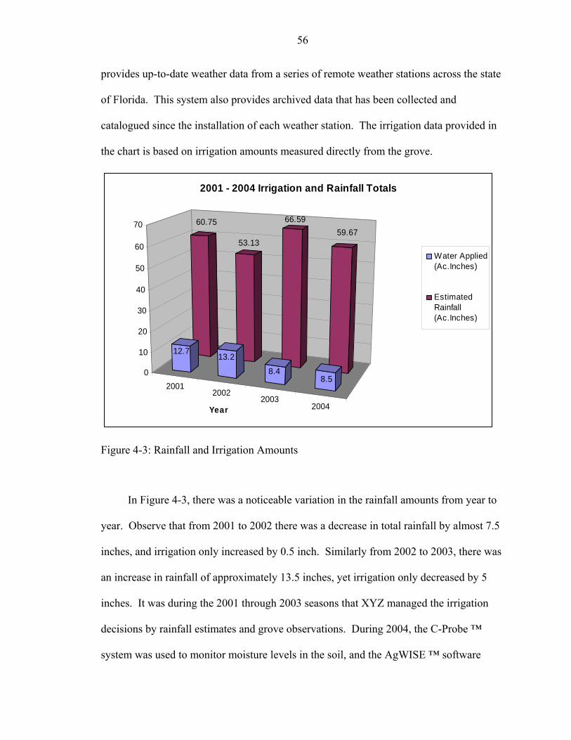
56
provides up-to-date weather data from a series of remote weather stations across the state
of Florida. This system also provides archived data that has been collected and
catalogued since the installation of each weather station. The irrigation data provided in
the chart is based on irrigation amounts measured directly from the grove.
20012002
20032004
60.75
53.13
66.5959.67
12.713.2
8.48.5
0
10
20
30
40
50
60
70
Year
2001 - 2004 Irrigation and Rainfall Totals
Water Applied(Ac.Inches)
EstimatedRainfall(Ac.Inches)
Figure 4-3: Rainfall and Irrigation Amounts
In Figure 4-3, there was a noticeable variation in the rainfall amounts from year to
year. Observe that from 2001 to 2002 there was a decrease in total rainfall by almost 7.5
inches, and irrigation only increased by 0.5 inch. Similarly from 2002 to 2003, there was
an increase in rainfall of approximately 13.5 inches, yet irrigation only decreased by 5
inches. It was during the 2001 through 2003 seasons that XYZ managed the irrigation
decisions by rainfall estimates and grove observations. During 2004, the C-Probe ™
system was used to monitor moisture levels in the soil, and the AgWISE ™ software
57
managed the data in irrigation templates. In 2004, there was a decline in rainfall by
roughly 7 inches from the previous year, yet irrigation remained constant. Recall in
2002, with a marked decrease in rainfall, the irrigation system was turned on more
frequently to make-up for the lack of rain. In 2004, this same scenario occurred but there
was not an “irrigate reaction” on the part of the grove manager. Ultimately since the
grove manager could now visualize the moisture levels in the soil column, there were
little to no unnecessary irrigations. This ability to monitor the moisture levels in the soil
allowed the grove manager to make more effective decisions about when and how much
to irrigate this grove.
Coinciding with the ability to make more effective decisions regarding the
timeliness of irrigations, XYZ was able to eliminate some expenses related to irrigation
control. From 2003 to 2004, there was a decrease by 5.5-percent in the amount of labor
required to manage the irrigation system, providing a cost savings of approximately $200.
Likewise, there was a savings of approximately $4,200 in fuel expenses related to
running the irrigation pumps. Not only was there a cost savings realized by the grove
owner, but the ability to more effectively irrigate resulted in a marked increase in crop
yield from that grove. The analysis on the irrigation system adoption differed greatly
from the VRT adoption due to the nature of the equipment. The irrigation and moisture
control system is composed of both fixed equipment costs as well as variable equipment
costs related to the number of C-Probes ™ required to operate effectively. This being the
case, per hectare cost of production is not as easily reported as seen in the VRT adoption
analysis previously in this chapter.
58
Discussion
The VRT fertilizer system is now being used on approximately 550 hectares of
total managed production area of approximately 2,300 hectares. They have not moved
their entire management area into VRT application at this time. From a management
perspective they feel that this would not be a wise decision since not all of their managed
groves have the tree size variability issues. They still maintain fixed-rate applications on
their properties that have consistent tree size and ages. It is also worth noting that XYZ
has encountered a decrease in VRT spreader effectiveness of properties and groves that
have an increased topographic profile. The less hills and inclines are better suited for the
effectiveness of the VRT in distributing the fertilizer.
In Chapter 2, there was a discussion related to the scale of the grove being a
determinant in the adoption of precision farming technologies. Data for Plot B provided
in Table 4-2 was only a 4 hectare (10 acre) grove. This scenario of contracting services
from a caretaker who utilizes precision farming technologies, allows the smaller grove
owners to now “adopt” a once unachievable level of technology. The costs of a VRT
system are quite high when compared to the holdings of a relatively small grove owner.
With regard to the irrigation and moisture control system, there are still some fine-
tuning concerns that the grove manager is focusing on, yet they are equally pleased with
the cost savings and water savings related to its installation. The grower made the
investment in this technology adoption, but providing greater irrigation control to XYZ
resulted in a single year improvement in internal fruit quality.
References made to Agrilink, C-Probe ™and AgWISE ™ were used only to
identify technology adoptions made by the grower/caretaker in this case study. There are
in no way a positive referral by the investigator in this study.
59
CHAPTER 5 CONCLUSIONS
Survey Analysis and Probit Model Results
This study investigated the current level of adoption of precision farming
technologies in Florida citrus production. To date, no study had been done on adoption
levels in Florida citrus. Secondly the study identified the demographic characteristics and
variables that determined the willingness to make the investment decision in these
technologies, by Florida citrus producers.
The most frequently adopted technologies were the sensor-based variable rate
applicators, soil variability mapping, and GPS boundary mapping. The least commonly
used technologies were remote sensing (e. g., aerial or satellite imagery) with its current
level of adoption and "prescription map" variable rate controllers. With regard to reasons
for non-adoption, the most common response was that producers were satisfied with their
current production practices, for all of the investigated technologies. The next most
common responses were lack of information regarding the respective technologies, and
lack of capital in order to make the investment in new technologies. The largest
percentage of the respondents indicated that, “I normally wait to see other's success with
new technologies and production methods.”
The probit model analysis determined that the variables most likely to influence the
willingness to adopt precision farming technologies were:
• Grower age: a negative correlation to the willingness to adopt
60
• Maximum and moderate variability: marginal probabilities indicate that farmers are more likely to adopt the technology compared to those in the minimum variability group.
Lastly, the probit model accurately predicted adoption decisions 73.3 percent of the
time. In addition, Type II error predictions resulting in a mistaken decision to invest only
occurred 8.9 percent of the time.
Case Study Analysis
In an effort to expound upon the “who” and “how many” have adopted, a case
study analysis investigated the “why” and “how” an individual firm in the citrus
production industry made the adoption decision. Citrus Caretakers, Inc. has a VRT
fertilizer system that is now being used on approximately 550 hectares (1,350 acres) of
their total managed production area. Collectively they manage approximately 2,300
hectares (5,600 acres) of groves that they both own and/or manage through direct
partnerships and contracts. They have not moved their entire management area into VRT
application at this time, and have only implemented its use on groves that have tree size
and density variability issues.
The breakeven analyses performed on Plot A and B were treated as though they
were owned by separate independent growers. This allowed for the analyses to determine
what the breakeven production area would need to be in order for the cost of the
investment to be recovered during each production year. In addition it is worth noting
that a small to medium-sized grower with an entrepreneurial spirit could use this
investment opportunity to create a custom application service in order to fill the excess
capacity required to breakeven on the investment by hiring themselves out to other small
growers.

61
With regard to the irrigation and moisture control system, CCI feels that there are
still some fine-tuning concerns that the grove manager is focusing on, yet they are
equally pleased with the cost savings and water savings related to its installation. The
grove owner made the investment in this technology adoption, but providing greater
irrigation control to CCI resulted in a single year improvement in fruit quality. This
positive change in fruit quality netted an immediate return on that investment by doubling
the total marketable yield.
Discussion and Closing Remarks
There are three criteria that must be met in order to justify the investment and
adoption of site-specific technologies. First, there must be a significant in-grove level of
variability, which affects crop yield. Second, this in-grove variability must be identified
and quantified. Lastly, the variability measured must be handled by the modification of
production practices and strategies in order to increase profit and decrease environmental
impacts (Plant, 2001).
In citrus, depending on the production region, in-grove variability may be rather
minimal. The case study analyzed in Chapter 4 of this study, identified a grove for
irrigation moisture control analysis, in which there were nine differentiable soil types, yet
all were various types of sand. As far as management practices were concerned for the
caretaker in that study, they were all managed as a single consistent soil type. There are
regions within the state’s production areas that do encounter varying soil types that must
be managed separately. This soil variability would be one qualifying criterion for
technology adoption, as long as the caretaker can measure and quantify the variability.
The third criterion for adoption seems to be problematic though. As indicated from the
survey results in Chapter 2 of this study, more than 60-percent of the respondents for
62
each of the ten technologies investigated, indicated that they were “satisfied with their
current practices”. This nullifies the third criterion identified by Plant (2001), that in
order to adopt, you must be willing to adapt and modify production management
strategies.
Referring back to the case study analysis in Chapter 4, Grove XYZ decided to
adopt a variable rate fertilizer spreader for the sole purpose of resolving tree size and
density issues. They encountered an issue that may be representative of a large
production area of the state. With the onslaught of hurricanes that Florida faced in 2004,
there was a significant amount of tree damage seen across the state. As a result, many
grove owners and caretakers began removing damaged trees and placing resets into those
damaged groves. As XYZ realized, a VRT fertilizer system using an “eye” sensor system
became an immediate solution to handling the fertilization of properties having
inconsistent tree sizes and densities. This adoption did however coincide with the need to
replace a worn and obsolete single-rate fertilizer applicator, so there was an economic
consideration and need before the adoption was made. Likewise as noted in the case
study, XYZ only uses this VRT fertilizer system on groves that “need” the varied
application rates.
The adoption of precision farming technologies is still in the “Early Adopter”
category with regard to Florida citrus production. As indicated in Chapter 2, the survey
results from the citrus producer survey show that only 18-percent of the respondents were
using one of the ten investigated precision farming technologies. On the other hand, 62-
percent of those respondents report their willingness to wait on other growers’ success
with the ten technologies. It is believed that the development of more generally accepted
63
mechanical harvesting systems (with yield monitoring capabilities) will induce a higher
willingness to adopt precision farming technologies. Yield monitoring has been the
highest percentage of adoption in the production of conventional cropping systems.
Identifying areas of high or low yield can assist in the measurement and observation of
in-grove variability. This in turn would assist in the adoption of VRT fertilization
systems.
Further investigation needs to be performed on the geographic distribution of
precision farming adopters. There may be some correlation between the growers’
location and their willingness to adopt, especially where certain SSCM equipment cannot
be used on very hilly terrain. In addition to the study on the geographic distribution of
adopters, research needs to be done on comparing fresh fruit producers versus processed
fruit producers. It is unlikely that there is a large percentage of precision farming adopters
associated with citrus production moving through fresh fruit marketing channels.
In addition, follow-up case studies should be performed on more precision
technology adopters, in order to cross-compare the success of the adoption decision
between those growers. Getting this information into publication outlets in the citrus
industry may assist in future adoptions by other growers.
The largest potential for immediate options appears to be the VRT sensor-based
fertilizer systems and chemical sprayers. In real-time, they have the ability to apply
varying levels of chemical inputs on trees of varied size and density. This in turn results
in an immediate savings with regard to inputs and the cost of total production per acre.
The technology with the second greatest potential for adoption would likely be
mechanized harvesters with on board yield monitoring capabilities. In production areas

64
where soil type is the least favorable for optimal moisture control, joint systems such as
C-Probe ™ and AgWISE ™, are an additional technologies that should be considered for
adoption.
65
APPENDIX A FLORIDA CITRUS GROWER TECHNOLOGY ADOPTION SURVEY
The following six pages represent the actual survey questionnaire that was
distributed and used to collect data for this study.
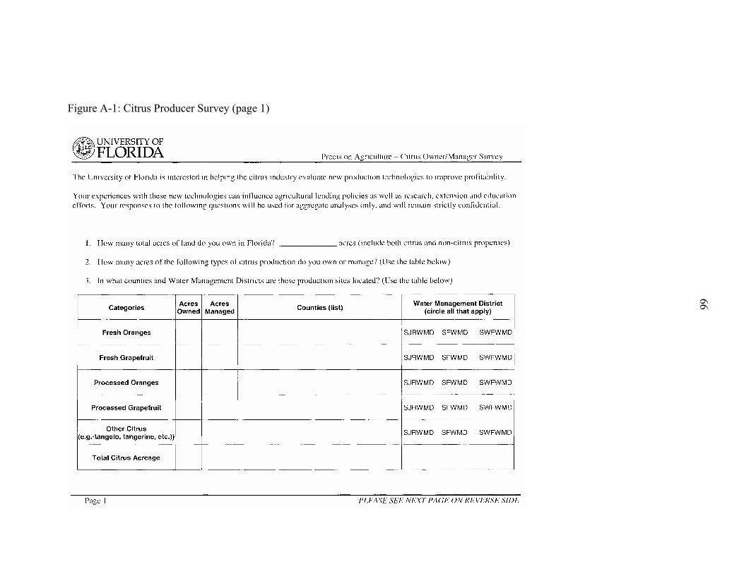
66
Figure A-1: Citrus Producer Survey (page 1)
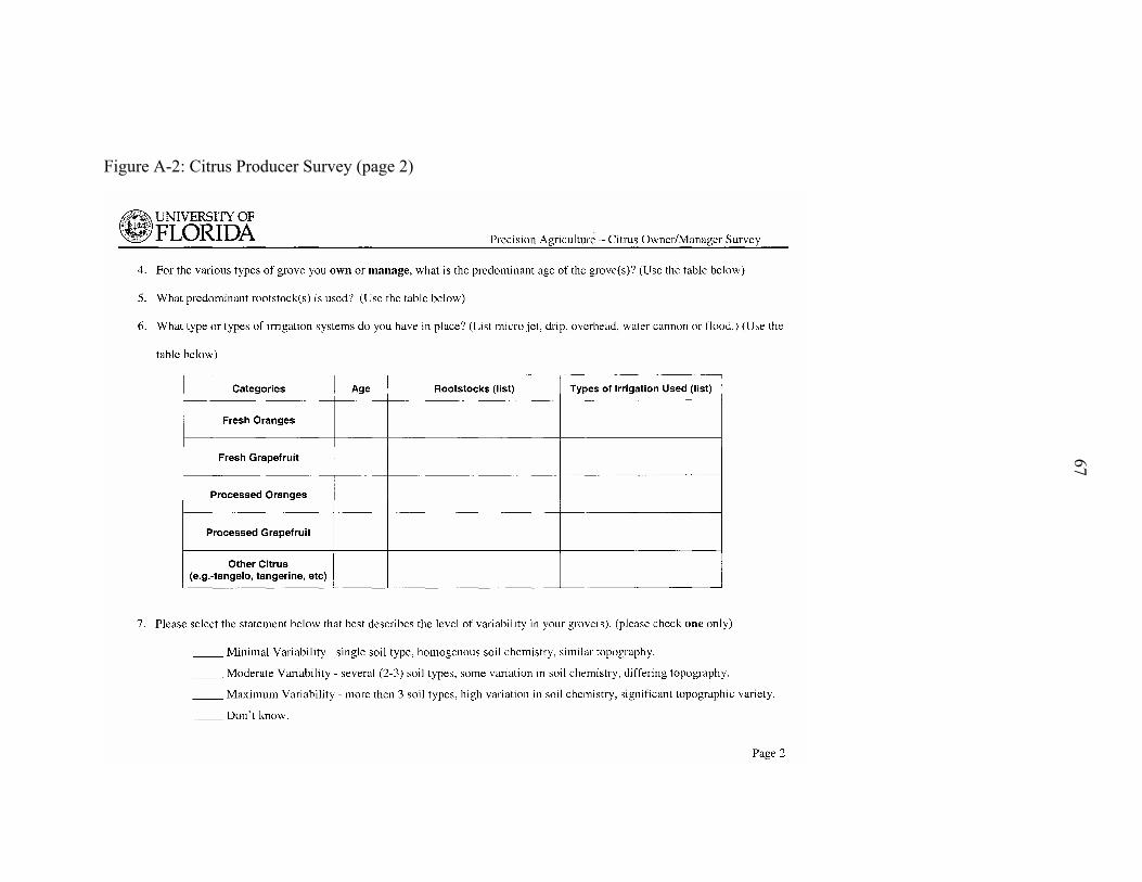
67
Figure A-2: Citrus Producer Survey (page 2)
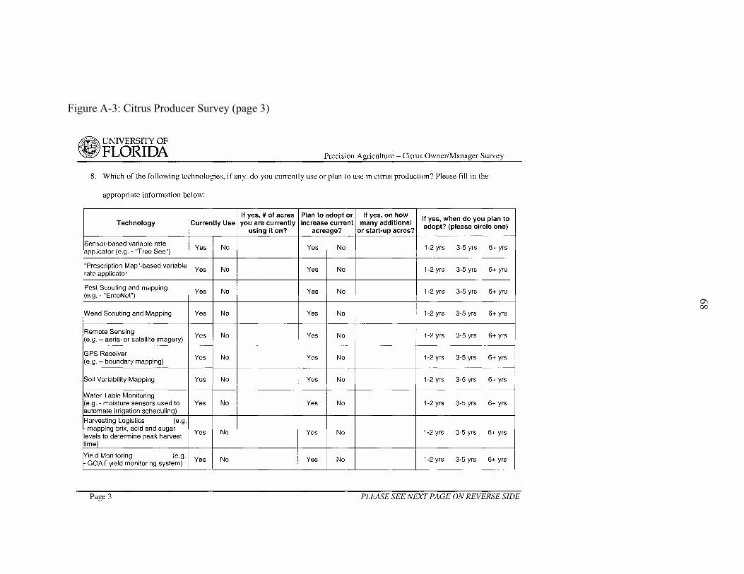
68
Figure A-3: Citrus Producer Survey (page 3)
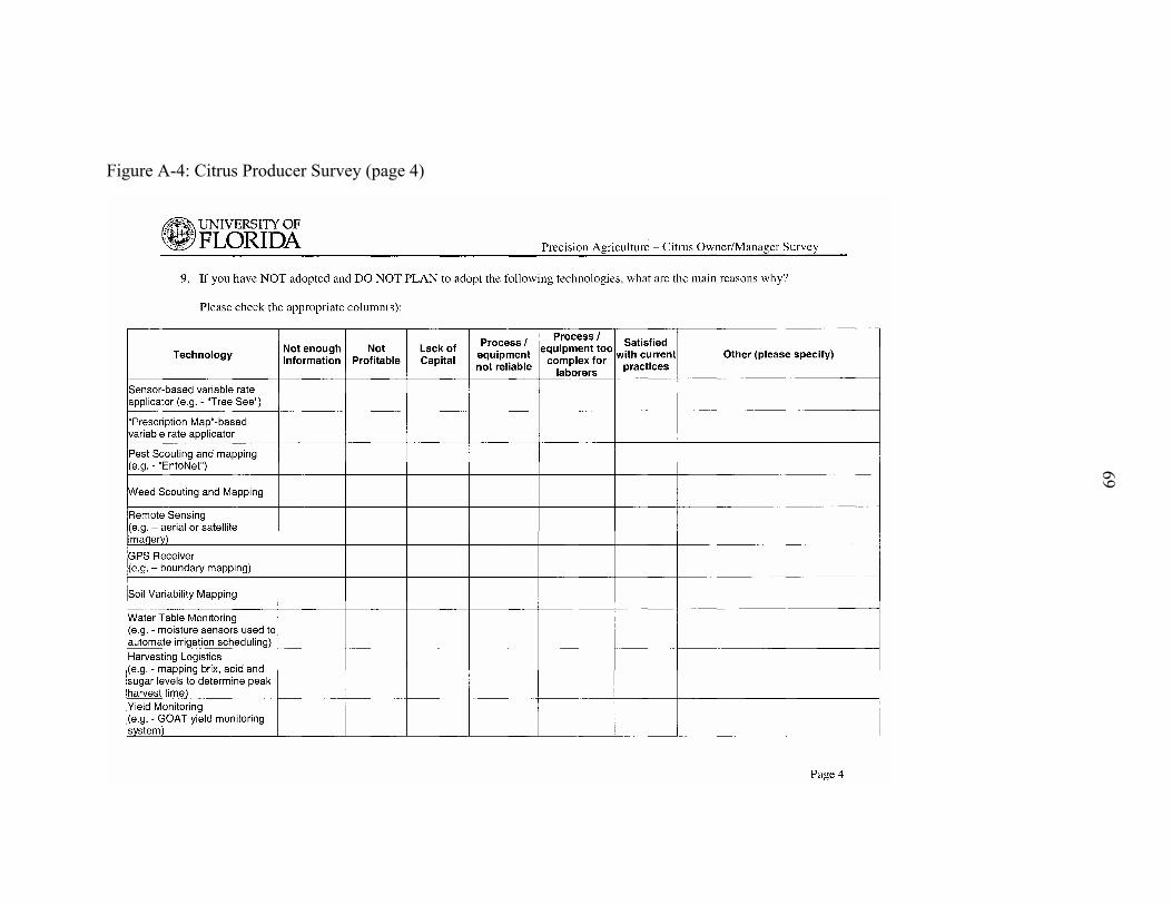
69
Figure A-4: Citrus Producer Survey (page 4)

70
Figure A-5: Citrus Producer Survey (page 5)
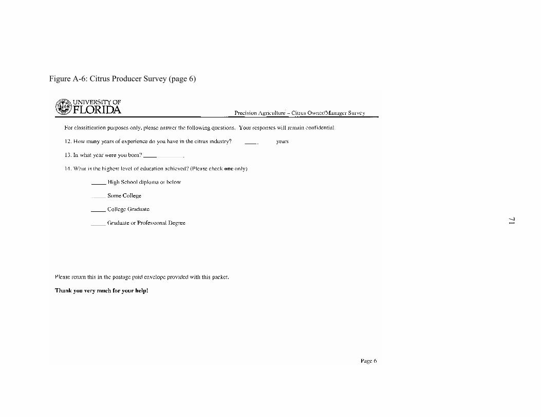
71
Figure A-6: Citrus Producer Survey (page 6)
72
APPENDIX B PROBIT MODEL ANALYSIS RESULTS
The probit model analysis was performed using the statistical software package
LIMDEP, version 7.0 (Greene, 1995).

73
+-----------------------------------------------------------------------+
| Dependent variable is binary, y=0 or y not equal 0 |
| Ordinary least squares regression Weighting variable = none |
| Dep. var. = USETECH Mean= .4370370370 , S.D.= .4978672035 |
| Model size: Observations = 135, Parameters = 10, Deg.Fr.= 125 |
| Residuals: Sum of squares= 26.19664518 , Std.Dev.= .45779 |
| Fit: R-squared= .211296, Adjusted R-squared = .15451 |
| Model test: F[ 9, 125] = 3.72, Prob value = .00036 |
| Diagnostic: Log-L = -80.8808, Restricted(b=0) Log-L = -96.9029 |
| LogAmemiyaPrCrt.= -1.491, Akaike Info. Crt.= 1.346 |
+-----------------------------------------------------------------------+
+---------+--------------+----------------+--------+---------+----------+
|Variable | Coefficient | Standard Error |b/St.Er.|P[|Z|>z] | Mean of X|
+---------+--------------+----------------+--------+---------+----------+
TC_OWN .1611888556E-04 .11095516E-04 1.453 .1463 837.61296
AGE .2975581064E-03 .24367421E-02 .122 .9028 58.696296
YRS_EXP -.3942252586E-02 .36000163E-02 -1.095 .2735 29.733333
LIKEADT .3048825378 .13132816 2.322 .0203 .185185
WAITADT .2893071501E-01 .10880994 .266 .7903 .651851
SOMEED .3212441544 .12816781 2.506 .0122 .237037
BSED .3302916708 .11808518 2.797 .0052 .481481
GRADED .3544126782 .14818655 2.392 .0168 .148148
MODVAR .2004367428 .85718669E-01 2.338 .0194 .414814
MAXVAR .3588914937 .12008715 2.989 .0028 .170370

74
+---------------------------------------------+
| Binomial Probit Model |
| Maximum Likelihood Estimates |
| Dependent variable USETECH |
| Weighting variable ONE |
| Number of observations 135 |
| Iterations completed 8 |
| Log likelihood function -71.23216 |
| Restricted log likelihood -92.50165 |
| Chi-squared 42.53899 |
| Degrees of freedom 9 |
| Significance level .2618101E-05 |
+---------------------------------------------+
+---------+--------------+----------------+--------+---------+----------+
|Variable | Coefficient | Standard Error |b/St.Er.|P[|Z|>z] | Mean of X|
+---------+--------------+----------------+--------+---------+----------+
Index function for probability
TC_OWN .4390390174E-03 .26705878E-03 1.644 .1002 837.61296
AGE -.1642453096E-01 .79138701E-02 -2.075 .0379 58.696296
YRS_EXP -.7439444811E-02 .11309781E-01 -.658 .5107 29.733333
LIKEADT .5686880888 .41653625 1.365 .1722 .185185
WAITADT -.1338363165 .34040528 -.393 .6942 .651851
SOMEED .6193040949 .39873538 1.553 .1204 .237037
BSED .5153843892 .37667667 1.368 .1712 .481481
GRADED .7517915387 .47205160 1.593 .1112 .148148
MODVAR .4308330425 .25950603 1.660 .0969 .414814
MAXVAR .8486323138 .39455804 2.151 .0315 .170370
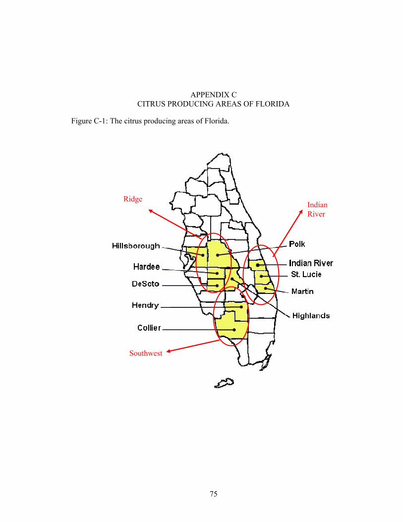
75
APPENDIX C CITRUS PRODUCING AREAS OF FLORIDA
Figure C-1: The citrus producing areas of Florida.
Ridge Indian River
Southwest
76
LIST OF REFERENCES
Agrilink Holdings Pty Ltd. 2005. http://www.agrilink-int.com . Australia.
AgWISE ™. 2005. http://www.agwise.net. Agrilink Holdings Pty Ltd. Australia.
Annamalai, P. and W.S. Lee. 2003. Citrus yield mapping using machine vision. ASAE Paper No. 031002. St. Joseph, MI.: ASAE.
Annamalai, P., W.S. Lee, and T.F. Burks. 2004. Color visions system for estimating citrus yield in real-time. ASAE Paper No. 043054. St. Joseph, MI.: ASAE.
Batte, M.T. and M.W. Arnholt. 2003. Precision farming adoption and use in Ohio: case studies of six leading-edge adopters. Computers and Electronics in Agriculture. 38 (2003): 125-139.
Brown, G.K. 2002. Mechanical harvesting systems for the Florida citrus juice industry. ASAE Paper No. 021108. St. Joseph, MI.: ASAE.
Daberkow, S. 1997. Adoption rates for selected crop management practices: Implications for precision farming. Choices. 3rd Quarter, 1997: 26-30.
Daberkow, S., and W. D. McBride. 1998. Socioeconomic profiles of early adopters of precision agriculture technologies. J. of Agribusiness. 16,2 (Fall 1998): 151-168.
Daberkow, S., and W. D. McBride. 2003. Farm and operator characteristics affecting the awareness and adoption of precision agriculture technologies in the US. Precision Agriculture. 4 (2003): 163-177.
D’Souza, G., D. Cyphers, and T. Phipps. 1993. Factors affecting the adoption of sustainable agricultural practices. Agr. and Res. Econ. Rev. October, 1993: 159-165.
Easterling, W.E., N. Chhetri, and X. Niu. 2003. Improving the realism of modeling agronomic adaptation to climate change: simulating technological substitution. Climatic Change. 60 (2003): 149-173.
Fisher, D.K., J. Norvell, S. Sonka, and M.J. Nelson. 2000. Understanding technology adoption through system dynamics modeling: implications for agribusiness management. Intl. Food & Agribus. Mgmt. Rev. 3 (2000) 281-296.
77
Florida Agricultural Statistics Service (FASS). 2002. Commercial Citrus Inventory - 2002. Orlando, FL: Florida Department of Agriculture and Consumer Affairs and USDA-Agricultural Marketing Service and National Agricultural Statistics Service.
Florida Agricultural Statistics Service (FASS). 2003. Citrus Summary 2002 - 2003. Orlando, FL: Florida Department of Agriculture and Consumer Affairs and USDA-Agricultural Marketing Service and National Agricultural Statistics Service.
Florida Automated Weather Network (FAWN). 2005. http://fawn.ifas.ufl.edu/ .University of Florida, Institute of Food and Agricultural Sciences.
Fowler, F. J., Jr. 2002. Survey Research Methods, 3rd ed. Thousand Oaks, CA: Sage Publications.
Geroski, P.A. 2000. Models of technology diffusion. Research Policy. 29 (2000): 603-625.
Greene, W. H. 1990. Models for Binomial Outcomes - Probit and Logit Models. In Econometric Analysis. 662-713. New York, NY: Macmillan Publishing.
Greene, W.H. 1995. LIMDEP Version 7.0. Bellport, NY: Econometric Software.
Grubler, A. 1998. Technology and global change. Cambridge: Cambridge Univ Press.
Jackson, L. K. and F. S. Davies. 1999. Citrus Growing in Florida. 4th ed. Gainesville, FL: University Press of Florida.
Katz, E. 1961. The social itinerary of technical change: two studies on the diffusion of innovation. Human Organization. 20 (1961): 70-82.
Kennedy, P.L. and E.J. Luzar. 1999. Toward methodological inclusivism: the case for case studies. Rev. of Agric. Econ. 21 (2) 1999: 579-591.
Khanna, M. 2001. Sequential adoption of site-specific technologies and its implications for nitrogen productivity: A double selectivity model. Amer. J. Agr. Econ. 83 (1): 35-51.
Khanna, M. ,O.F. Epouhe, and R. Hornbaker. 1999. Site-specific crop management: adoption patterns and trends. Rev. of Agric. Econ. 21 (2) 1999: 455-472.
Khanna, M., M. Isik, and A. Winter-Nelson. 2000. Investment in site-specific crop management under uncertainty: implications for nitrogen pollution control and environmental policy. Agricultural Economics. 24 (2000): 9-21.
Long, J. Scott. 1997. Regression Models for Categorical and Limited Dependent Variables. Thousand Oaks, CA: Sage Publications.
78
Maddala, G.S. 1983. Limited-Dependent and Qualitative Variables in Econometrics. New York, NY: Cambridge University Press.
Miller, W.M. and J.D. Whitney. 2003. A test program to assess VRT granular fertilizer applications for citrus. ASAE Paper No. 031126. St. Joseph, MI.: ASAE.
Morgan, M., and D. Ess. 2003. The Precision-Farming Guide for Agriculturists; 2nd. edition. Moline, IL: John Deere Publishing.
Moore, G.A. 1991. Crossing the Chasm. New York, NY: Harper Business.
Muraro, R. P., and W. C. Oswalt. 2002. Budgeting costs and returns for central Florida citrus production, 2001-02. Food and Resource Economics, Economic Information Report EI 02-9. Gainesville, FL: University of Florida.
Muraro, R. P., F. M. Roka, and R. E. Rouse. 2002a. Budgeting costs and returns for southwest Florida citrus production, 2001-02. Food and Resource Economics, Economic Information Report EI 02-10. Gainesville, FL: University of Florida.
Muraro, R. P., J. W. Hebb, and E. W. Stover. 2002b. Budgeting costs and returns for Indian River citrus production, 2001-02. Food and Resource Economics, Economic Information Report EI 02-11. Gainesville, FL: University of Florida.
National Research Council (NRC). 1997. Precision agriculture in the 21st century: geospatial and information technologies in crop management. Washington, DC: National Academy Press.
Plant, R.E. 2001. Site-specific management: the application of information technology to crop production. Computers and Electronics in Agric. 20 (2001): 9-29.
Rogers, E.M. 1962. Diffusion of Innovations. New York, NY: The Free Press of Glencoe, Macmillan.
Rogers, E.M. 2003. Diffusion of Innovations; 5th ed.. New York, NY. The Free Press.
Ruttan, V.W. 1959. Usher and shumpeter on invention, innovation, and technological change. Qaurt. Journal of Econ. 73 (1959): 596-606.
Ryan, B. and N.C. Gross. 1943. The diffusion of hybrid seed corn in two Iowa communities. Rural Sociology. 8 (1943):15-24.
Schueller, J.K., J.D. Whitney, T.A. Wheaton, W.M. Miller, and A.E. Turner. 1999. Low-cost automatic yield mapping in hand-harvested citrus. Computers and Electronics in Agric. 23 (1999): 145-153.
Townsend, C. 2004.Irrigation templates for Florida citrus. Proc. Fla. State Hort Soc. 117 (2004):100-103.

79
Wei, J. and M. Salyani. 2004. Development of a laser scanner for measuring tree canopy characteristics: Phase 1 prototype development. Trans. of ASAE. 47 (6) 2004: 2101-2107.
Whitney, J.D., Q. Ling. W.M. Miller, and T.A. Wheaton. 2001. A DGPS yield monitoring system for Florida citrus. Applied Eng in Agric. 17 (2) 2001: 115-119.
Yin, R.K. 2003. Case Study Research Design and Methods, 3rd ed. Thousand Oaks, CA: Sage Publications.
80
BIOGRAPHICAL SKETCH
Brian James Sevier, born September 1974, in Salisbury, Maryland, is seeking the
degree of Doctor of Philosophy in the College of Agriculture and Life Sciences,
agricultural operations management, in the Agricultural and Biological Engineering
Department.
Brian completed his Masters of Agribusiness (MAB) from the University of
Florida, Food & Resource Economics Department in 2000. Brian also received his
Bachelor of Science (BS) in food and resource economics specializing in agribusiness
management, as well as a minor in business administration from the University of Florida
in 1999.
Brian currently is employed by the University of Florida, Food and Resource
Economics Department as a Coordinator, Economic Analysis. In this position he serves
as the Department’s Business and Operations Manager.
Brian was married to wife Danielle in 1997, and they have a son Tristan, who was
born in 2002.