Optimal Space Lower Bounds for all Frequency Moments David Woodruff Based on SODA 04 paper.
Portfolio Selection and Lower Partial Moments
Alexander Wojt
Royal Institute of Technology Department of Mathematics
Stockholm, Sweden


Abstract
In this thesis lower partial moments (LPM) are introduced as risk measures in portfolio optimization (mean-LPM optimization). LPM has several features making it a more suitable risk measure for the investor compared to variance. Empirical tests will be carried out to compare mean-variance optimization with mean-LPM optimization. The results will be discussed in light of a robustness analysis under a resampled efficiency framework (Michaud, 1998) performed in order to discuss the models´ sensitivities to estimation errors.

V
Table of Contents
1 Introduction ................................................................................................................................... 1
2 The Concept of Risk and Return .................................................................................................. 3
2.1 Rate of Return ....................................................................................................................... 3
2.2 Risk Measures ....................................................................................................................... 4
2.2.1 Value at Risk and Expected Shortfall ....................................................................... 6
2.2.2 Lower Partial Moments ............................................................................................ 7
3 Classical Portfolio Theory ........................................................................................................... 11
3.1 Deriving the Efficient Frontier ............................................................................................ 12
3.2 Duality ................................................................................................................................. 15
3.3 Limitations of Classical Portfolio Theory ........................................................................... 17
4 Beyond Classical Portfolio Theory ............................................................................................. 19
4.1 The Need for a New Theory ................................................................................................ 19
4.2 Mean-LPM Portfolio Theory ............................................................................................... 20
4.3 Utility Theory ...................................................................................................................... 23
4.3.1 Utility Theory and Classical Portfolio Theory ....................................................... 23
4.3.2 Utility Theory and Mean-LPM Portfolio Theory ................................................... 25
4.4 Multi-Period Mean-Variance Optimization ........................................................................ 28
5 Empirical Tests ............................................................................................................................ 31
5.1 Data .................................................................................................................................... 31
5.2 Back-Testing Mean-Variance Portfolio Theory and Mean-LPM Portfolio Theory ........... 32
VI
6 Robustness Analysis .................................................................................................................... 39
6.1 Robustness .......................................................................................................................... 39
6.2 Resampling .......................................................................................................................... 43
6.3 The Black-Litterman Model ................................................................................................ 50
6.4 Shrinkage Estimation of the Covariance Matrix ................................................................. 58
7 Conclusions................................................................................................................................... 64
7.1 Conclusions ........................................................................................................................ 64
7.2 Future Analysis................................................................................................................... 65
References ............................................................................................................................................ 66

VII
Acknowledgments
I would like to thank my supervisor Filip Lindskog for his ideas and guidance throughout the preparation of this thesis. I am also grateful to my family and friends for their continuous support.

VIII

1
Chapter 1
Introduction
In the beginning of the last century, Louis Bachelier published his PhD thesis, “Theory of Speculation” at Sorbonne, Paris (Bachelier, 1900). It was the first time someone had tried to develop ideas in finance with rigorous mathematics. His thesis came to be a prominent work upon which many of the financial models and theories of today are partly built. Among these theories is the portfolio theory developed by Harry Markowitz (1952). Markowitz was a pioneer in the field of quantitative portfolio selection and was awarded the Nobel Prize in 1990. Using his model an investor can weight his portfolio in a way that maximizes the expected return for a given risk.
This breakthrough was a major step forward for financial mathematics. The theory did however not meet the same enthusiasm outside academia. Practitioners often found the resulting set of asset weights unintuitive and thus did not consider the model a practical tool for investment purposes. This is one of the main dilemmas with portfolio theory and the idea with this thesis is to find a way to bring portfolio theory closer to practitioners.
More specifically, the aim of this thesis is to look at an alternative risk measure and examine whether it could be suitable for portfolio optimization. Markowitz used variance as measure of risk in his original paper but in this thesis variance will be replaced by lower partial moments (LPM). The hypothesis is that the theoretical benefits of using lower partial moments that will be discussed will yield satisfactory results when the model is tested on historical data. The change of risk measure will furthermore allow for a relaxation of the normal distribution assumption necessary when using variance as risk measure.
The entry of LPM in portfolio theory has mainly been driven by Bawa (1975), Fishburn (1977) and Nawrocki (1991, 1992 and 1999). This thesis can partly be seen as a development of their ideas.
The outline of this thesis is as follows: In Chapter 2 the concepts of risk and return are introduced. In Chapter 3 classical portfolio theory is derived and discussed. In Chapter 4 mean-LPM portfolio theory is introduced. In Chapter 5 empirical tests are simulated. In Chapter 6 a robustness analysis is performed on the methods used in Chapter 5. In Chapter 7 summary and conclusions are stated.

2
3
Chapter 2
The Concept of Risk and Return
There is a saying that goes “there is no such thing as a free lunch”, meaning that if an investor wants higher returns he needs to take on lager risks. There is however no clear-cut definition of risk. Intuitively, risk is something that takes into account the probability as well as the severity of an event. People know that to win they need to bet, and to win big they need to bet a lot. In financial terms, large returns are often associated with large risks. Harry Markowitz was the first person to quantify this risk – return relationship in an optimization framework that came to be the foundation of modern portfolio theory (Markowitz, 1952). Using his theory an investor can pick out assets and weight his portfolio to maximize the expected portfolio return for a given portfolio risk. At the core of the theory lies the understanding of risk and return. In this chapter the rate of return and different ways of measuring risks will be introduced. This will encompass the basis needed for a comprehensive understanding of the portfolio theory that will be developed in later chapters.
2.1 Rate of Return
Portfolio theory is about maximizing the return for a given risk. The natural way of measuring return
is by first defining the initial value 0V of a portfolio.
0 010
n k
kkV h S
== ≥∑
1( ,..., )nh h=h is a vector with the units of the
n assets held in the portfolio. Notice that some
elements in h can be negative, that is, short selling is to some extent allowed. The value of asset k at
time t is k
tS . The vector of asset values at this time can be expressed as
1( ,..., )n
t tS S=
tS . The value of
the portfolio at time 1t = is
1 11
n k
kkV h S
==∑
4
The weight and the return of asset k can be expressed as
0
0
k
kk
h S
Vω =
1 0
0
k k
k k
S Sr
S
−=
The portfolio return pr can now be written in the following way
1 0 0 1 01 0 1 1
10 0 0 0
( ) ( )n n
k k k k k
k k nTk k
p k kkk
h S S h S S SV V
r rV V V S
ω= =
=
− −−
= = = = =∑ ∑
∑ ω r
1( ,..., )T
nω ω=ω 1( ,..., )T
nr r=r
The way that returns are normally measured is pretty straightforward. The value of the portfolio today is compared with the value of the portfolio yesterday, the percentage change is the return of the portfolio. This is the most common way to measure returns of portfolios and it will be the choice of measure for the rest of this thesis. It should however be mentioned that there are other ways of measuring returns, for example by use of upper partial moments (Cumova et al., 2004) which however will not be discussed.
2.2 Risk Measures
In this section the topic of risk measurement will be discussed. In the portfolio theory developed by Markowitz risk is measured by standard deviation. Definition 1 Given a random variable X with expected value µ the standard deviation σ of
X is given by
2[( ) ]E Xσ µ= −
For a continuous distribution where the random variable X has a probability
density ( )p x the standard deviation can be expressed as
2( ) ( )x p x dxσ µ= −∫
with
( )xp x dxµ = ∫
The most frequently used estimator of σ is * 2
1
1( )
1
n
i
i
s x xn =
= −− ∑ where 1,..., nx x
is the sample
5
and 1
1 n
i
i
x xn =
= ∑ is its mean where n is the number of observations. Standard deviation is often used in
portfolio optimization as well as in other fields where a simple measure of risk is needed. Sometimes
variance is discussed instead of standard deviation and the two are related such that 2( )var X σ= .
Nonetheless, as Markowitz has argued (Markowitz, 1959) a better measure of risk ought to be variance below a certain reference point. Variance measures the variation around a mean. However, variations don´t necessarily have to be bad if they are above a certain threshold. To deal with this limitation of variance, semi-variance was introduced. Definition 2 If X is a random variable with cumulative distribution function ( )XF x
and the
reference level is τ , semi-variance is given by
2 2( ) (max( ,0) ) ( ) ( )X XSV F E X x dF x
τ
τ τ τ−∞
= − = −∫
It is intuitive that in the case of portfolio optimization downside risk should be minimized and not upside risk. Minimizing standard deviation would mean minimizing upside risk as well. The discussion of downside risk measures will continue by examining two commonly used downside risk measures, Value at Risk (VaR) and Expected Shortfall (ES). Companies face a wide range of risks. Let´s consider a company consisting of n units. The loss variable for the units will be 1,..., nL L and for the whole firm 1 ... nL L L= + + .
The amount of cash the company is required to hold (decided internally by risk management or externally by regulators) is decided by the risk measure ρ . Depending on how acceptable the risk is,
the firm must hold a certain amount of buffer capital. If the risk is acceptable 0ρ ≤ shall hold and if
not, 0ρ ≥ is the additional amount of capital that needs to be added to the buffer capital for the risk to be acceptable. Different families of risk measures have been defined but one of the families of measures that frequently appear in the literature is the family of coherent risk measures (Acerbi et al., 2001). A coherent risk measure is supposed to be a “good” measure of risk, in the sense that it has four desirable properties. Definition 3 A risk measure ρ is called a coherent risk measure if it satisfies Axiom 1-4 where
1Z and 2Z
are random variables.
Axiom 1 – Monotonicity If 1 2Z Z≤ then 1 2( ) ( )Z Zρ ρ≥
Axiom 2 – Sub-Additivity 1 2 1 2( ) ( ) ( )Z Z Z Zρ ρ ρ+ ≤ +
Axiom 3 – Positive Homogeneity If 0α ≥ then ( ) ( )Z Zρ α αρ=
Axiom 4 – Translation Invariance If α ∈R then ( ) ( )Z Zρ α ρ α+ = −

6
Convex risk measures constitute another family of risk measures that were introduced by Föllmer and Scheid (2002). According to their definition convex risk measures take into account the fact that large positions may be exposed to liquidity risk. If a position is increased the risks may increase in a non-linear way. To deal with this Föllmer and Scheid relaxed Axiom 2 and 3 in Definition 3 and replaced them with a convexity axiom
Axiom 5 – Convexity 1 2 1 2( (1 ) ) ( ) (1 ) ( )Z Z Z Zρ λ λ λρ λ ρ+ − ≤ + − for any (0,1)λ∈
Axiom 1, 4 and 5 together defines a convex risk measure. In this thesis different risk measures will be discussed and they will not necessarily be convex or coherent.
2.2.1 Value at Risk and Expected Shortfall
During the last 20 years one of the most popular ways for financial institutions to assess risk has been through Value at Risk (VaR). VaR measures the worst expected loss given a certain confidence level and time horizon. For example, a portfolio with a VaR equal to $1 million given a confidence level of 5% and a time horizon of one week means that the probability that the loss of the portfolio will exceed $1 million in one week is less than 5%. VaR can furthermore be expressed more formally.
Definition 4 Assume that the stochastic loss X follows the distribution XF . Given (0,1)α ∈ ,
( )VaR Xα is given by the smallest number x so that the probability that the loss X
exceeds x is not greater than 1 α− .
( ) inf : ( ) 1VaR X x P X xα α= ∈ > ≤ −R
inf :1 ( ) 1Xx F x α= ∈ − ≤ −R
inf : ( )Xx F x α= ∈ ≥R
The measure grew in popularity among professionals because of its simplicity and could often (and still can) be found on the financial statements of major financial institutions. However, in 1999 VaR was for the first time sharply criticized in the article by Artzner et al. (Artzner et al., 1999) where the definitions of a coherent measure of risk were outlined (Definition 3). VaR does not satisfy the sub-additivity axiom and use of VaR could thereby lead to excess risk taking. VaR could for example suggest that diversification should be decreased in order to reduce risk, something that contradicts empirical tests and fundamental financial theory. Because of the limitations and the weaknesses of VaR new ways of assessing risk have emerged. One such way which has slowly started to get foothold outside academia is expected shortfall (also called Tail Expected Loss or Conditional Value at Risk). Instead of looking at what is likely to happen, expected shortfall (ES) takes into account how bad things will go when they will really go bad. This is done by examining the conditional expectation and investigating the expected loss of a portfolio when the loss is bigger than a certain threshold value. Definition 5 Given the stochastic loss X and (0,1)α ∈ Expected Shortfall (ES) is given by
( ) ( | ( ))ES X E X X VaR Xα α= ≥

7
A common way to rewrite the expression for ES is
[ ( ), ]
[ ( ), ]
( )
( ) ( | ( ))
( ( ))
( ( ))
1( ( ))
1
1( )
1
q X
q X
X
q X
ES X E X X VaR X
E X X
P L q L
E X X
xdF x
α
α
α
α α
α
α
α
∞
∞
∞
= ≥
Ι=
≥
= Ι−
=− ∫
where
[ ( ), ]
1 ( )( )
0 ( )q X
for X q XX
for X q Xα
α
α∞
>Ι =
≤
As was the case with VaR, ES returns an easily interpreted value that gives the investor a sense of how bad things can go. Risk management is often focused on extreme risks that can ruin a company or a portfolio, and these risks are captured in ES. A more general definition of ES is given by General Expected Shortfall (GES) which is not limited to the case where the stochastic loss X follows a continuous distribution. Definition 6 Consider the stochastic loss X . If (0,1)α ∈ General Expected Shortfall (GES) is
given by
( )[ ( ), ]
1( ) ( ( )) ( )(1 ( ( )))
1 q XGES X E X X q X P X q Xαα α αα
α ∞= Ι + − − ≥−
GES is a coherent risk measure along the lines of Definition 3. Furthermore, when the distribution of
the stochastic loss X is continuous it holds that ( ) ( )ES X GES Xα α= .
There are several other measures of risks than VaR or ES, but for asset managers VaR and ES have played an important role and it is vital to understand their strengths and weaknesses when discussing other risk measures and their use in portfolio optimization. Before discussing portfolio optimization another risk measure will be introduced, lower partial moments. In later chapters the differences between portfolio optimization based on variance and lower partial moments will be analyzed.
2.2.2 Lower Partial Moments
The concept of moments in mathematics originally comes from the world of physics. Mean and variance are moments of the first and second order but it is possible to make a more general definition of moments.
8
Definition 7 If X is a random variable with cumulative distribution function ( )XF x and
reference level τ the moment of degree n is
, ( ( )) (( ) ) ( ) ( )n n
n X XF x E X x dF xτµ τ τ∞
−∞
= − = −∫
The special case when the reference level τ equals the mean of the distribution is called the central moment. The first moment around zero is thus the mean of the distribution and the second central moment is the variance. Normalized central moments are also introduced
,
(( ) )( ( ))
n
n X n
E XF xτ
τµ
σ−
=
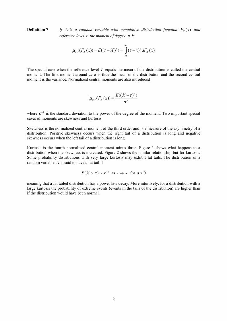
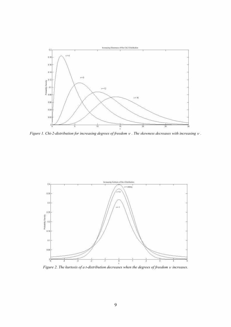
where nσ is the standard deviation to the power of the degree of the moment. Two important special cases of moments are skewness and kurtosis. Skewness is the normalized central moment of the third order and is a measure of the asymmetry of a distribution. Positive skewness occurs when the right tail of a distribution is long and negative skewness occurs when the left tail of a distribution is long. Kurtosis is the fourth normalized central moment minus three. Figure 1 shows what happens to a distribution when the skewness is increased. Figure 2 shows the similar relationship but for kurtosis. Some probability distributions with very large kurtosis may exhibit fat tails. The distribution of a random variable X is said to have a fat tail if
( ) ~P X x x α−> as x → ∞ for 0a > meaning that a fat tailed distribution has a power law decay. More intuitively, for a distribution with a large kurtosis the probability of extreme events (events in the tails of the distribution) are higher than if the distribution would have been normal.
9
Figure 1. Chi-2-distribution for increasing degrees of freedom ν . The skewness decreases with increasing ν .
Figure 2. The kurtosis of a t-distribution decreases when the degrees of freedom ν increases.
10
So far the general definition of moments and some of their features have been considered. Lower Partial Moments (LPM) can be said to be to moments what semi-variance is to variance. LPM simply examines the moment of degree n below a certain threshold τ . LPM was first defined by Fishburn (Fishburn, 1977) Definition 8 If τ is a chosen reference level, n is the degree of the moment and X is a random
variable with cumulative distribution ( )XF x the Lower Partial Moments (LPM)
are given by
, ( ) (max( ,0) ) ( ) ( )n n
n X XLPM F E X x dF x
τ
τ τ τ−∞
= − = −∫
In practice LPM can for m observations be estimated by the following expression
*, , ,
1
1(max(0, ))
mn
n i i t
t
LPM Xm
τ τ=
= −∑
LPM is a family of risk measures specified by τ and n . τ is often set to the risk free rate or simply to zero. By choosing the degree of the moment an investor can specify the measure to suit his risk aversion. Intuitively, large values of n will penalize large deviations more than low values. Semi-variance is a special case of LPM for which the degree of the moment is set to two.
11
Chapter 3
Classical Portfolio Theory
In previous chapters the theory necessary to derive and understand classical portfolio theory (mean-variance portfolio theory) was outlined. This is a theory of investment which explains how an investor should weight his portfolio to maximize the return for a given risk. In the original paper of Markowitz (Markowitz, 1952) the risk measure used is variance. The consequences of using variance as risk measure will in detail be discussed later but the immediate advantage is that the mathematical derivation will be rather straightforward. Mean-variance portfolio theory as discussed in Markowitz (Markowitz, 1952) rests on a set of assumptions.
1. Short-selling is allowed. 2. Investors are rational and risk averse. 3. There are no transaction costs or bid-ask spreads. 4. The size of a position in an asset is not limited. 5. Investors care only about the risk and the return of assets.
6. The return vector r is multivariate normal distributed. The goal of each rational investor is either to minimize the risk (variance) for a chosen return or to maximize the return for a chosen level of risk. Later a proof will be derived showing that these problems (Problem 1 and Problem 2) lead to equivalent solutions. Problem 1:
Minimize the risk of the portfolio for a given expected portfolio return. Problem 2:
Maximize the expected return of the portfolio for a given portfolio risk. In these problems an additional constraint forcing the weights to sum to one will be added.
12
3.1 Deriving the Efficient Frontier
Before looking into the details of the optimal allocation problem some matrix algebra which will be used in this chapter is reviewed. If A and B are matrices, 1η and 2η are vectors and c is a scalar the following relations hold.
( )( )
( )
( )
TT
T T T
T T T
T T
A A
A B A B
AB B A
cA cA
=
+ = +
=
=
If A is invertible it holds that
1 1( ) ( )T TA A− −=
If A is symmetric it holds that
TA A= If A is invertible and symmetric it holds that
1 1 1 11 2 1 2 2 1 2 1( ) ( )T T T T T TA A A A− − − −= = =η η η η η η η η
The analytical solution of the optimization problem that comes with classical portfolio theory in the form of Problem 1 will now be derived1. Consider the single-period optimal allocation problem with 2n ≥ risky assets. The return of asset k is
kr and ( )E =r µ with 1( ,..., )T
nr r=r and 1( ,..., )T
nµ µ=µ . Thus, the expected portfolio return can
be written as ( )T T
pr E= =ω r ω µ . In mean-variance portfolio theory the measure of risk is variance,
1 1 ,1 1 1 1
( ) ( ... ) ( , )n n n n
p n n j j k k j k j k
j k j k
var r var r r cov r rω ω ω ω ω ω= = = =
= + + = = Σ∑∑ ∑∑
This can be expressed more compactly
1,1 1, 1
1
,1 ,
( ) ( ,..., )n
T
p n
n n n n
var r
ωω ω
ω
Σ Σ = = Σ
Σ Σ
ω ω
L
M O M M
L
1 The derivation of the theory and the discussion in this chapter is based on lecture notes by Filip Lindskog from the course “Portfolio Theory and Risk Management” taught in 2008 at the Royal Institute of Technology as well as lecture notes from the course “Financial Markets: Theory & Evidence”, taught by Thomas Renström in 2002 at the University of Rochester (http://www.econ.rochester.edu/Wallis/Renstrom/Eco217.html). The original analytical derivation of the problem can be found in Merton (1972).
13
Σ is the covariance matrix with , ,j k j k j kρ σ σΣ = and ,
cov( , )j k
j k
j k
r rρ
σ σ= . The optimal allocation
problem can now be formulated. The solution will return the vector of optimal asset weights * * *
1( ,..., )T
nω ω=ω .
Problem 1 can be expressed as a quadratic optimization problem (referred to as 1( )m v− for mean-
variance. Sub-index 1 refers to Problem 1)
The factor 1
2will make calculations easier and will not affect the optimization problem. The problem
can be solved analytically by forming the Lagrange function.
1 2 1 2
1( , , ) ( ) 1 )
2T T T
prγ γ γ γ= Σ + − + −L ω ω ω ω µ ( ω 1
1γ and 2γ are Lagrange multipliers. To find optimal weights the Lagrange function is differentiated
with respect to ω .
1 2 1 2( , , )γ γ γ γ∇ = Σ − −ωL ω ω µ 1
By letting this equal zero an expression for the optimal weights is found.
* 1 12 1γ γ− −= Σ + Σω 1 µ
Consequently, the conditions of the problem can be expressed in the following way
* 1 11 2
T T Tγ γ− −= Σ + Σµ ω µ µ µ 1
* 1 1
1 2T T Tγ γ− −= Σ + Σ1 ω 1 µ 1 1
Using the constraints, 1T =ω 1 and T
pr=ω µ , the equations above can be rewritten as
1 2pr a bγ γ= +
1 21 b cγ γ= +
where 1Ta −= Σµ µ ,
1Tb −= Σµ 1 and 1Tc −= Σ1 1 . 1γ and 2γ can now be explicitly expressed.
1
1min
2. . ( )
1
T
T
T
p
s t m v
r
Σ
− =
=
ω ω ω
ω 1
ω µ
14
1 2
pr c b
ac bγ
−=
− 2 2
pa r b
ac bγ
−=
−
If this is inserted in the expression for *ω an expression for the optimal portfolio weights is found.
1 1 1 1
* 1 1 11 22 2 2 2
( )p p
p
r c b a r b b b c br g g
ac b ac b ac b ac b
− − − −− − −− − Σ − Σ Σ − Σ
= Σ + Σ = + = Σ +− − − −
1 µ µ 1ω µ 1 µ 1
where
1 2
pcr bg
ac b
−=
− 2 2
pa brg
ac b
−=
−
This is the solution to the problem 1( )m v− . By inserting the optimal portfolio weights in the
expression for variance the relationship between mean and variance of optimal portfolios when the expected portfolio return varies can be examined.
2*2 * *
2
2p pTcr br a
ac bσ
− += ∑ =
−ω ω
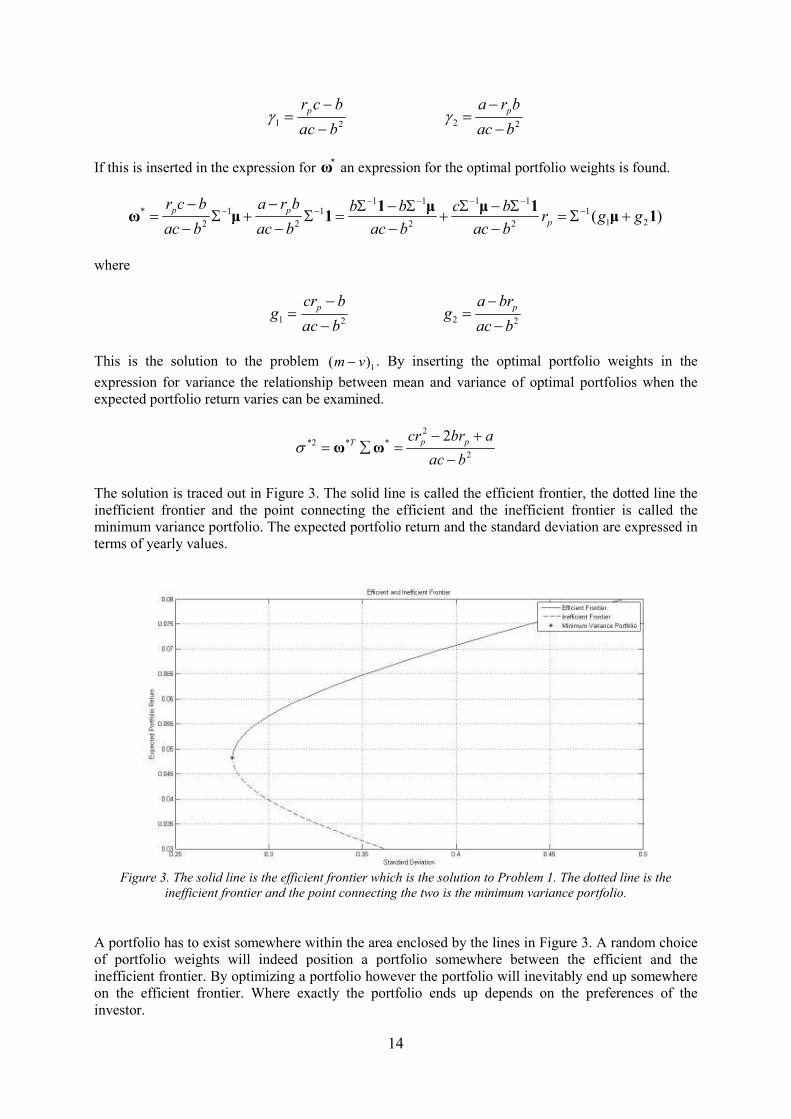
The solution is traced out in Figure 3. The solid line is called the efficient frontier, the dotted line the inefficient frontier and the point connecting the efficient and the inefficient frontier is called the minimum variance portfolio. The expected portfolio return and the standard deviation are expressed in terms of yearly values.
Figure 3. The solid line is the efficient frontier which is the solution to Problem 1. The dotted line is the
inefficient frontier and the point connecting the two is the minimum variance portfolio.
A portfolio has to exist somewhere within the area enclosed by the lines in Figure 3. A random choice of portfolio weights will indeed position a portfolio somewhere between the efficient and the inefficient frontier. By optimizing a portfolio however the portfolio will inevitably end up somewhere on the efficient frontier. Where exactly the portfolio ends up depends on the preferences of the investor.
15
3.2 Duality
As mentioned earlier, Problem 1 and Problem 2 are equivalent in the sense that they have the same solution, the problems are said to be dual. Duality is a common feature in optimization theory and it is often useful when trying to find solutions that need less computations. Problem 2 can be solved in a similar way that Problem 1 was solved. The optimization problem 2( )m v− is written as
The Lagrange function is formed
21 2 1 2( , , ) ( ) (1 )T T T
pλ λ λ σ λ= + − Σ + −L ω ω µ ω ω ω 1
The Lagrange function is differentiated with respect to ω . By letting this equal zero an expression for the optimal weights is derived.
1 2 1 2
1 2
* 1 121 2
1 1
( , , ) 2 0
2
1( ) ( )2 2
f f
λ λ λ λ
λ λ
λλ λ
− −
∇ = − Σ − =
⇒ Σ = −
⇒ = Σ − = Σ +
ωL ω µ ω 1
ω µ 1
ω µ 1 µ 1
This looks similar to the solution of the problem 1( )m v− . When 1 1f g= and 2 2f g= the problems
should lead to equivalent solutions. The Lagrange multipliers 1λ and 2λ are found by inserting *
ω in
the equations for the constraints.
1 1 1*
2 2 21 1 1
1 12 2
1 1
2 1
( ) ( ) ( )2 2 2
1 1( ) ( ) 1
2 2
1( 2 )
T T
T T T T
T T b c
bc
λ λ λλ λ λ
λ λλ λ
λ λ
− − −
− −
Σ Σ Σ= − = − = −
= Σ − Σ = − =
⇒ = −
ω 1 µ 1 1 µ 1 1 µ 1 1
µ 1 1 1
The second constraint can now be used to find a second relation between 1λ and 2λ .
2
2
max
. .( )
1
T
T
T
p
s tm v
σ
−=
Σ =
ω ω µ
ω 1
ω ω

16
[ ]2
1 1
2 2
1 1
1
1 1 1* *
2 2 2 21 1 1 1
1 1 1 1 2 12 2 2 22 2
2 2 22 2 22 2
2
1( ) ( ) ( ) ( )
2 2 2 2
1 1
4 4
1 12
4 4
1
4
T T
T T
T T T T T T
pa b b c a b c
λ λ λ λλ λ λ λ
λ λ λ λ λλ λ
λ λ λ λ λ σλ λ
λσ
− − −
− − − − −
Σ Σ ΣΣ = − Σ − = − −
= − Σ − = Σ − Σ − Σ + Σ
= − − + = − + =
⇒ =
ω ω µ 1 µ 1 µ 1 µ 1
µ 1 µ 1 µ µ µ 1 1 µ 1 1
2
1 1
1 1
1 1 1
22
2 1 12 2
2 2 2 2211
2 2
2 22 2 22 2 2 2 2 2
1 1 12 2 ( 2 ) ( 2 )
4
4 4 42 41 1
4 4
4 4 44 4 (4 )
p p
p p
p p p
a b c a b b c bc c
b b bb ba a
c c c
b b ba a a
c c c c c c
λ λ λ λσ
λ λ λλσ σ
λ λσ λ σ λ λ σ
− + = − − + −
− + − − = − + = −
⇒ = − + ⇒ − = − ⇒ − = −
1
2
2 22
12 2 21 4( 1) 4( 1)4 p p p
ac b
ac b ac bc
c c c
c
λ λσ σ σ
−− −
⇒ = = ⇒ =− − −
This is inserted in the expression for 2λ
2 2
2 1 2 2
1 2 1( 2 )
4( 1) 1p p
b ac b ac bb b
c c c c c cλ λ
σ σ
− −= − = − = −
− −
Finally, inserting 1λ and 2λ in the expression for the optimal weights a deterministic expression for the
optimal weights is found.
2
2
* 1 12
2 21 1
2 2
2 2 2 221 1
2 2 2 2 2
1
( 1)1 1( )2 2
2 24 1 4 1
1 1 1 11 11
1
p
p p
p p p p
p
ac bb
c c
ac b ac b
c c
c c c cac bb b
ac b c ac b c ac b c ac b
σλλ λ
σ σ
σ σ σ σ
σ
− −
− −
− −
− = Σ − = Σ − − −
− −
− − − −− = Σ − − = Σ + − − − − − −
ω µ 1 µ 1
µ 1 µ
( )11 2f f−
= Σ +
1
µ 1
As mentioned before, the problems 1( )m v− and 2( )m v− yield the same solution when
1 1f g= and 2 2f g= . Using the first relation yields
17
2 2 2 2 2 2 22 2
2 2 2 2 2
1 ( ) 2 21
( )p p p p p p p
p p
c cr b cr b c r bcr b ac b cr br ac
ac b ac b ac b c bc a ac b
σσ σ
− − − − + + − − += ⇒ − = ⇒ = =
− − − − −
This relation is the same as the relation found when solving the problem 1( )m v− . The same result is
obtained by using 2 2f g= . The proof is completed, 1( )m v− and 2( )m v− have the same solution.
3.3 Limitations of Classical Portfolio Theory
Two of the limitations of classical portfolio theory will now be discussed. First (i), the use of means and variances in portfolio theory is not always feasible. In fact it can be shown that this is only reasonable when the distribution of r is approximated by a multivariate normal distribution or if the investor has a quadratic utility function. If the distribution of r is approximated by a multivariate normal distribution an investor will only have to observe the mean and variance, there is nothing else he can observe even if he wanted to. If the investor has a quadratic utility function he won´t care about other factors than means and variances, even if they did exist (e.g. higher moments). This will be covered in more detail in Chapter 4.3. Second (ii), the covariance matrix Σ and the mean vector µ are not observable and have to be estimated. This is often done using historical data. However, one cannot use too old data since it will be irrelevant and a bad prediction of an asset´s future movement. Thus investors are often forced to use less data which could lead to large estimation errors. This will be covered in more detail in Chapter 6. By replacing variance as measure of risk the normality assumptions in classical portfolio theory will be relaxed. The first step is to introduce portfolio optimization with LPM as measure of risk.

18

19
Chapter 4
Beyond Classical Portfolio Theory
In the last chapter the concept of portfolio theory was developed and in the end some of its limitations were discussed. The questions that now have to be answered are; “is classical portfolio theory good
enough?” and second; “if it is not good enough, what can we do about it?”. These questions will be answered with the limitation (i) of classical portfolio theory in mind from the discussion in Chapter 3.3.
4.1 The Need for a New Theory
Initially the first question from the last paragraph will be addressed. If asset returns were normally distributed the variance and the mean would be the only parameters an investor would need in order to describe the distribution. To be more specific, the return vector r must be multivariate normally distributed. The random space Z has a multivariate normal distribution if its components
kZ are
independent and if ~ (0,1)kZ N . A random vector 1( ,..., )T
nX X=X has a multivariate normal
distribution with mean 1( ,..., )T
nµ µ=µ and covariance matrix Σ if
A= +X µ Z
where A satisfies the relation TAA = Σ . If this would be the case and if empirical tests would confirm
this then mean-variance portfolio theory would not suffer from limitation (i). However, the assumption that the distribution of the return vector is multivariate normally distributed is not always supported by empirical tests. To better understand how to test whether an asset has a normal distribution one of the most common tests will be made on the return of the currency pair USD/FJD (United States Dollars to Fiji Dollars). A Q-Q-plot is a graphical method to compare two distributions with one another. What is done is basically that the quantiles of two distributions are plotted against one another. Similar distributions will plot along a straight line. However, comparing our unknown distribution with the normal distribution a normal probability plot which relies on the same theory as the Q-Q-plot will be used. The data set will be plotted against a theoretical normal distribution and if the distribution is normal it should result in the data being plotted
20
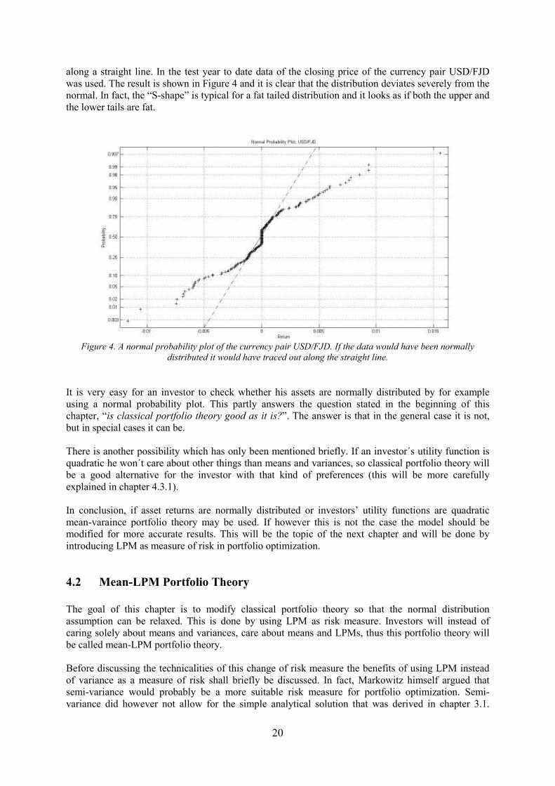
along a straight line. In the test year to date data of the closing price of the currency pair USD/FJD was used. The result is shown in Figure 4 and it is clear that the distribution deviates severely from the normal. In fact, the “S-shape” is typical for a fat tailed distribution and it looks as if both the upper and the lower tails are fat.
Figure 4. A normal probability plot of the currency pair USD/FJD. If the data would have been normally
distributed it would have traced out along the straight line. It is very easy for an investor to check whether his assets are normally distributed by for example using a normal probability plot. This partly answers the question stated in the beginning of this chapter, “is classical portfolio theory good as it is?”. The answer is that in the general case it is not, but in special cases it can be. There is another possibility which has only been mentioned briefly. If an investor´s utility function is quadratic he won´t care about other things than means and variances, so classical portfolio theory will be a good alternative for the investor with that kind of preferences (this will be more carefully explained in chapter 4.3.1). In conclusion, if asset returns are normally distributed or investors’ utility functions are quadratic mean-varaince portfolio theory may be used. If however this is not the case the model should be modified for more accurate results. This will be the topic of the next chapter and will be done by introducing LPM as measure of risk in portfolio optimization.
4.2 Mean-LPM Portfolio Theory
The goal of this chapter is to modify classical portfolio theory so that the normal distribution assumption can be relaxed. This is done by using LPM as risk measure. Investors will instead of caring solely about means and variances, care about means and LPMs, thus this portfolio theory will be called mean-LPM portfolio theory. Before discussing the technicalities of this change of risk measure the benefits of using LPM instead of variance as a measure of risk shall briefly be discussed. In fact, Markowitz himself argued that semi-variance would probably be a more suitable risk measure for portfolio optimization. Semi-variance did however not allow for the simple analytical solution that was derived in chapter 3.1.
21
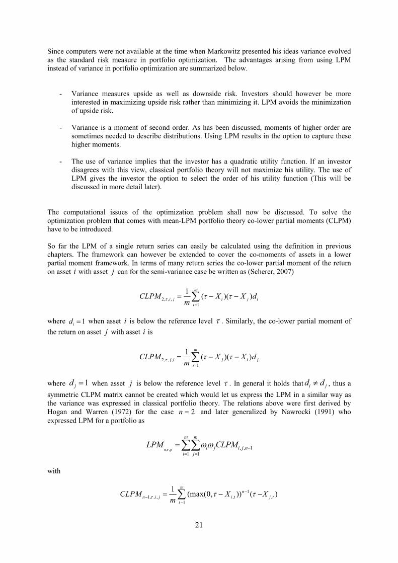
Since computers were not available at the time when Markowitz presented his ideas variance evolved as the standard risk measure in portfolio optimization. The advantages arising from using LPM instead of variance in portfolio optimization are summarized below.
- Variance measures upside as well as downside risk. Investors should however be more interested in maximizing upside risk rather than minimizing it. LPM avoids the minimization of upside risk.
- Variance is a moment of second order. As has been discussed, moments of higher order are
sometimes needed to describe distributions. Using LPM results in the option to capture these higher moments.
- The use of variance implies that the investor has a quadratic utility function. If an investor disagrees with this view, classical portfolio theory will not maximize his utility. The use of LPM gives the investor the option to select the order of his utility function (This will be discussed in more detail later).
The computational issues of the optimization problem shall now be discussed. To solve the optimization problem that comes with mean-LPM portfolio theory co-lower partial moments (CLPM) have to be introduced. So far the LPM of a single return series can easily be calculated using the definition in previous chapters. The framework can however be extended to cover the co-moments of assets in a lower partial moment framework. In terms of many return series the co-lower partial moment of the return on asset i with asset j can for the semi-variance case be written as (Scherer, 2007)
2, , ,1
1( )( )
m
i j i j i
i
CLPM X X dm
τ τ τ=
= − −∑
where 1id = when asset i is below the reference level τ . Similarly, the co-lower partial moment of
the return on asset j with asset i is
2, , ,1
1( )( )
m
j i j i j
i
CLPM X X dm
τ τ τ=
= − −∑
where 1jd = when asset j is below the reference level τ . In general it holds that i jd d≠ , thus a
symmetric CLPM matrix cannot be created which would let us express the LPM in a similar way as the variance was expressed in classical portfolio theory. The relations above were first derived by Hogan and Warren (1972) for the case 2n = and later generalized by Nawrocki (1991) who expressed LPM for a portfolio as
, , , , 11 1
n p
m m
i j i j n
i j
LPM CLPMτ
ωω −= =
=∑∑
with
11, , , , ,
1
1(max(0, )) ( )
mn
n i j i t j t
t
CLPM X Xm
τ τ τ−−
−
= − −∑

22
As mentioned above, CLPM is in general not symmetric. This implies that
1, , , 1, , ,n i j n j iCLPM CLPMτ τ− −≠ i j≠
However, as Nawrocki (1991) shows, calculating CLPM as a symmetric measure yields good results,
and since it will make computations easier his assumption will be used. This means that the CLPM
between two assets can be expressed in terms of LPM as
( )1
* *, , , , , , , ,
nn i j n i n j i jCLPM LPM LPMτ τ τ ρ=
Where ,i jρ is the correlation between asset i and asset j . Recalling how the variance was expressed
,1 1
( )m m
T
p j k j k
j k
var r ω ω= =
= Σ = Σ∑∑ ω ω
It is clear that LPM can be expressed as
, , 1, , ,1 1
n p
m mT
i j n i j
i j
LPM CLPM Lτ τωω −
= =
= =∑∑ ω ω
where sub-index p refers to the LPM for the portfolio. Furthermore the matrix L is introduced
1, ,1,1 1, ,1,
1, , ,1 1, , ,
n n m
n m n m m
CLPM CLPM
L
CLPM CLPM
τ τ
τ τ
− −
− −
=
L
M O M
L
The optimization problem that should be solved can now be written as
. .( )
1
T
T
p
T
min L
s tm LPM
r
−=
=
ωω ω
ω µ
ω 1
Since L is symmetric the problem is almost identical to the one solved in the case of mean-variance optimization. The only difference is that the covariance matrix is replaced by the matrix L.

23
4.3 Utility Theory
Utility theory is a theory about ranking levels of wealth. It has slowly been changing the framework of portfolio theory by focusing on the maximization of expected utility instead of on the maximization of return for a given risk. In a sense, to work with utility in portfolio theory gives the investor more choice to shape a portfolio in a way that will maximize his personal utility. In this chapter the basics behind utility theory will be explained. It will also be shown how mean-LPM portfolio optimization goes hand in hand with expected utility maximization. Consider a utility function ( )u x where x is wealth and ( )u x can be thought of as the “happiness” of
owning x . A utility function will in general be concave, reflecting the fact that investors experience diminishing marginal utility. This means that the wealthier a person is, the less an extra dollar will improve his utility. Thus the following must hold, as for all concave functions
( (1 ) ) ( ) (1 ) ( )u ax a y au x a u x+ − ≥ + − (0,1)a∈
Furthermore, ( )u x should be twice differentiable and in general, ( ) 0u x ≥ and ´ ( ) 0u x ≤ . The Arrow-Pratt measure of absolute risk aversion r is moreover defined as
´ ( )( )
( )
u cr c
u c= −
This measure explains how the risk aversion changes with the level of wealth. For example,
( ) ln( )u x x= implies that 1
rx
= meaning that the risk aversion declines the wealthier an investor is2.
The certainty equivalent C is also defined
( ) ( ( ))u C E u X=
Thus the amount that can be gotten for certain,C , has the same level of utility as the expected utility of the amount X .
It should be noticed that in general the absolute values given by utility functions cannot really be interpreted; instead the utilities of wealth are ranked. Next it will be shown that classical portfolio theory is congruent with an investor with quadratic utility function3 and later that mean-LPM portfolio theory offers much more variety for investors.
4.3.1 Utility Theory and Classical Portfolio Theory
The return pr of a portfolio can in a one period model be expressed as T
pr =ω r . This means that the
value of the portfolio at time 1t = will have grown from 0V to 0 1(1 )TV V+ =ω r . This implies that
the optimization problem of interest in the expected utility framework is
2 Example taken from D. G. Lueneberger, 1998, Investment Science, Oxford University Press, p.233 3 The theory behind this part is inspired by the lecture notes in the course Portfolio Theory and Risk Management, by Filip Lindskog at the Royal Institute of Technology, 2008.

24
0max ( (1 ))
. . ( )
1
T
T
E V
s t EU
+ =
ωω r
ω 1
where ( )EU stands for expected utility. By assuming that the investor has a quadratic utility function on the form
221( )
2
cu x c x= −
The expression for the expected utility function can be rewritten in the following way
222 0
0 1 0
222 0
1 0 1
2 22 22 0 2 0
1 0 1 0 2 0
22 21 0 1 0 2 0
2 0 2 22 0 2 0
( (1 )) (1 ) ((1 ) )2
(1 ) (1 )2
( ) ( )2 2
1 1 1( )
2 2 2
T T T
T T T
T T T
T T T
c VE V cV E E
c VcV cV E Var
c V c VcV cV c V
cV cV c Vc V
c V c V
+ = + − +
= + − + + +
= − + − − + Σ
−= − + − − Σ
ω r ω r ω r
ω µ ω r ω r
ω µ ω µ ω ω
ω µ ω µ ω ω
where the following relation was used
2 2 2( ) ( ) ( )var X E X E X= −
Introducing the constant
21 0 2 0
22 0
cV c V
c Vφ
−=
the expression for the expected utility can be written as
20
1 1( (1 )) ( )
2 2T T T TE V φ+ = − − Σω r ω µ ω µ ω ω
Hence the problem ( )EU can be rewritten as
21 1max ( )
2 2. . ( )
1
T T T
T
s t EU
φ − − Σ =
ω ω µ ω µ ω ω
ω 1

25
This optimization problem can be solved in exactly the same way as the duality problem in Chapter 3.2 was solved. To avoid tedious algebra the solution is simply stated. The optimal set of weights in the problem ( )EU will be identical to those in the problem 1( )m v− if the problem is solved for
2
2p
b ac b c br
c ac b c c
φ − − = + − +
Looking at this expression, b
c is identified as the expression for the minimum variance portfolio
shown in Figure 3. The expression for the variance when solving the problem 1( )m v− was
2
*2 * *2
2p pTcr br a
ac bσ
− += ∑ =
−ω ω
The minimum variance portfolio is found by letting the derivative equal zero and solving for pr .
*2
0 p
p
br
r c
σ∂= ⇒ =
∂
Thus the solution to the problem ( )EU is an efficient portfolio if b cφ > . To sum up, in this chapter it was shown that maximizing the expected utility of an investor with quadratic utility function yields the same optimal weights as when solving the mean-variance portfolio problem. In this sense, mean-variance portfolio theory is very limited, since it can only optimize portfolios of one kind of investors.
4.3.2 Utility Theory and Mean-LPM Portfolio Theory
In this chapter it will be shown that in the case of mean-LPM optimization, the investor is no longer forced to have one specific utility function. To realize how mean-LPM optimization and utility theory are related the article by Fishburn (1977) was studied where he developed this relation. Consider the distributions F and G . Furthermore, assume that the investor makes his investment decision entirely based on ( )Fµ , ( )Fρ , ( )Gµ and ( )Gρ where ρ is a risk measure and µ is the
mean of the distribution. Furthermore, consider a real valued function ( , )u µ ρ , increasing in µ and
decreasing in ρ . It holds that
F Gf if and only if
( ( ), ( )) ( ( ), ( ))u F F u G Gµ ρ µ ρ> where F Gf is read “F is preferred to G ”. The last relation should hold if and only if
( ) ( ) ( ) ( )x dF x x dG xψ ψ∞ ∞
−∞ −∞
>∫ ∫
26
where ( )xψ is a real-valued function. Then there exists constants 1c , 2c and 3c such that
1 2
1 2 3
( )( )n
c c x for xu x
c c x c x for x
ττ τ
+ ≥= + − − <
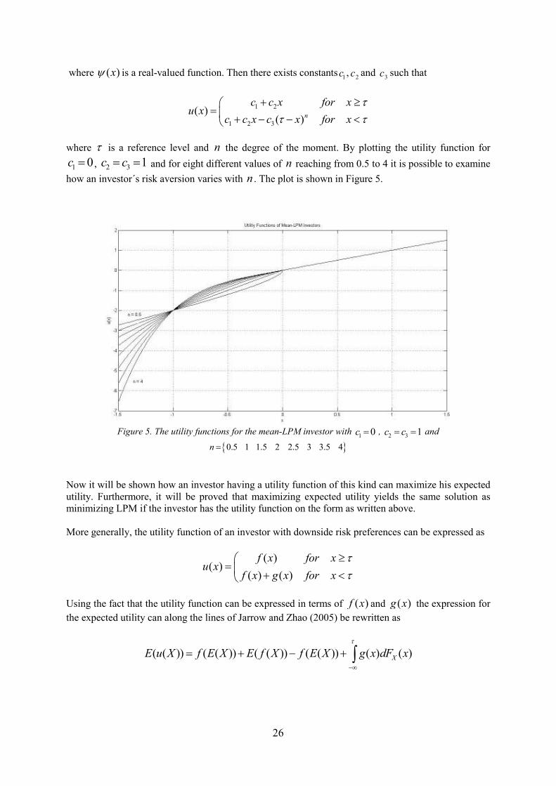
where τ is a reference level and n the degree of the moment. By plotting the utility function for
1 0c = , 2 3 1c c= = and for eight different values of
n reaching from 0.5 to 4 it is possible to examine
how an investor´s risk aversion varies with n . The plot is shown in Figure 5.
Figure 5. The utility functions for the mean-LPM investor with 1 0c = , 2 3 1c c= =
and
0.5 1 1.5 2 2.5 3 3.5 4n =
Now it will be shown how an investor having a utility function of this kind can maximize his expected utility. Furthermore, it will be proved that maximizing expected utility yields the same solution as minimizing LPM if the investor has the utility function on the form as written above. More generally, the utility function of an investor with downside risk preferences can be expressed as
( )( )
( ) ( )
f x for xu x
f x g x for x
ττ
≥= + <
Using the fact that the utility function can be expressed in terms of ( )f x and ( )g x the expression for the expected utility can along the lines of Jarrow and Zhao (2005) be rewritten as
( ( )) ( ( )) ( ( )) ( ( )) ( ) ( )XE u X f E X E f X f E X g x dF x
τ
−∞
= + − + ∫
27
Where X follows the distribution XF , ( ( ))f E X is a function of the expected return,
( ( )) ( ( ))E f X f E X− incorporates the risk in term of variation and ( ) ( )Xg x dF x
τ
−∞∫
is a measure of
downside risk. The calculations are simplified by defining
( ( )) ( ( )) ( ( ))f SD X f E X E f X= − where 2 2( ) ( ) ( )SD X E X E X= −
The downside risk measure of X following the distribution XF is defined as
( ) ( )X XDRM g x dF x
τ
−∞
= − ∫
Thus in the case where LPM is used as downside risk measure it holds that
, ( )X n XDRM LPM Fτ=
Now the expected utility can be rewritten
,( ( )) ( ( )) ( ( )) ( )n XE u X f E X f SD X LPM Fτ= − −
As mentioned before, the 1( )m v− problem will give the same solutions as when maximizing an
investor´s quadratic utility function. It can be shown that maximizing the expected utility expressed as above will give the same solutions as when solving the problem ( )m LPM− . That is, for the expected
utility function above the solution *ω will be the same for both optimization problems
max ( ( ))
. .( )
1
p
T
p
T
E u r
s tEU LPM
r
−=
=
ω
ω µ
ω 1
,min ( )
. .( )
1
n X
T
p
T
LPM F
s tm LPM
r
τ
−=
=
ω
ω µ
ω 1
Let´s look at the proof derived by Jarrow and Zhao (2005). Their proof holds not only for LPM but for all kinds of downside risk measures for which the utility function can be expressed in terms of ( )f x
and ( )g x as was done on the previous page.
Suppose that *pr solves ( )EU LPM− but not ( )m LPM− . Then there must exist a pr
• satisfying the
conditions shared by both problems such that *( ) ( )p pE r E r• ≥ , *( ) ( )p pSD r SD r• ≤ and
*, ,( ) ( )p p
n nr rLPM F LPM Fτ τ• ≤ . The expected utility can then be written as
,( ( )) ( ( )) ( ( )) ( )p
p p p n rE u r f E r f SD r LPM Fτ •
• • •= − −
28
Since f is increasing and f and LPM are non-decreasing, it must hold that *( ( )) ( ( ))p pE u r E u r• > .
This contradicts that *pr solves ( )EU LPM− . Thus, if a set of weights solve one of the problems they
will also solve the other one. Thus the m-LPM optimization is congruent with the maximization of expected utility. An investor does have some choice regarding his utility function and risk aversion in contrast to the case of classical portfolio optimization. The power utility function an investor experiences in the mean-LPM model is also more realistic than the quadratic utility function experienced by the 1( )m v− investor.
However, above the reference level τ the investor is assumed to be risk neutral. This is acknowledged as one of the mean-LPM model´s main weaknesses. In this chapter LPM was introduced as a risk measure in portfolio optimization instead of variance. As has been discussed, LPM has several features which make it superior as a risk measure to variance. It was moreover shown that using mean-LPM portfolio optimization allows the investor to have a wide range of utility functions which is a clear advantage to classical portfolio theory where investors are assumed to have quadratic utility functions.
4.4 Multi-Period Mean Variance Optimization
When deriving the optimization problem 1( )m v− in Chapter 3.1 the assumption that the investor
made his choice of weights at time 0t = and evaluated the result of the portfolio at time 1t = was made. Thus the problem was a single-period problem. In reality, investors often invest over longer time horizons where they will have to rebalance their portfolios according to movements in the markets and to new information. Because of this a multi-period model emerged and the topic has been developed by Smith (1967), Samuelson (1969) and lately by Li and Ng (2000) to name a few. Li and Ng (2000) extended the analytical solution of the single-period case to the more general multi-period model and our theoretical review will be based partly on their work and partly on Rudoy (2009). The aim of this chapter is to extend the theory of the single-period model in a natural way.
The objective for an investor will be to maximize terminal wealth given an equality constraint on the variance. In this formulation the budget constraint is relaxed to make calculations easier to follow. The optimization problem 1( )mp can be expressed as
0 1 1 0
0
1
, ,..., 10
1
12
1 00
max
. . ( )
var
N
NT
t k k
k
NT
t k k
k
E
s t mp
σ
−
−
+=
−
+=
=
∑
∑
ω ω ω ω r
ω r
Where 1k k k k −= ∆ = −r x x x and kx is the vector of asset values at period k . The problem 1( )mp
cannot be solved directly using dynamic programming techniques, however, as Li and Ng (2000) show a technique called the principle of separable embedding can be used that will yield the optimal portfolios. When using this technique a related problem 2( )mp is solved instead of directly solving the
problem 1( )mp .
29
0 1 1 0
21 1
, ,..., 1 1 20 0
max ( )N
N NT T
t N k k N k k
k k
E mpγ λ−
− −
+ += =
−
∑ ∑ω ω ω ω r ω r
The optimal weights 0 1 1, , ..., N −ω ω ω for the problem 2( )mp will be optimal for the problem 1( )mp
for an appropriate choice of Nγ and
Nλ . Furthermore, Rudoy (2009) identifies the value function
* 2( )N N N N N NJ r r rγ λ= −
where
1 1 1( )T
N N N N Nr r − − −= + −ω x x
The problem 2( )mp is rewritten below for the special case 1t N= −
( ) ( )( ) ( )( )
( ) ( )( )( )
1 1 1 1
1 1
1
1
2
2
1 1 1 1 1 1
21 1 1 1 1 1 1 1 1
1 1 1
max ( ) max
max ( ) ( )
max 2
max
N N N N
N N
N
N
t N N t N N N N
T T
t N N N N N N N N N N
TT T
N N N N N N N N N N N N N N N N
T
N N N N N N N
E J r E r r
E r r
r E r r E
r r
ω γ λ
γ λ
γ γ λ λ
γ γ λ
− − − −
− −
−
−
− − − − − −
− − − − − − − − −
− − −
= −
= + − − + −
= + − − − − −
= + −
ω
ω
ω
ω
ω x x ω x x
ω x x ω x x x x ω
ω m2
1 1 1 1 1 1 12 T T
N N N N N N N Nr Sλ λ− − − − − − −− −ω m ω ω
where
( )
( )( )( )1
1
1 1
1 1 1
N
N
N t N N
T
N t N N N N
E
S E
−
−
− −
− − −
= −
= − −
m x x
x x x x
The optimal set of weights is found by letting the derivative of the expression above equal zero and
solving for *1N−ω . This yields
( )* 11 1 1 1 1 1
12 ( ) ( )
2N N N N N N N N
N
r Sγ λλ
−− − − − − −= −ω x m x
Making the same calculations the solution for *2N−ω is found which is expressed in a similar way as
*1N−ω . By recursion it can be shown that in the general case,
( )* 11( , ) 2 ( ) ( )
2k k k N N k k k k k
N
r r Sγ λλ
−= −ω x x m x
with
30
( )( ) ( )( )( )( )( )( )
11 1 1 1
11 1 1 1 1
11 1 1 1 1 1
( )
( )
( )
k
k
k
T
k k t k k k k
T
k k t k k k k k k
TT
k k t k k k k k k k k
v E v S
E v S
S E v S
−+ + + +
−+ + + + +
−+ + + + + +
= −
= − −
= − − −
x m m
m x m m x x
x m m x x x x
To reach a solution for the problem 1( )mp a way to calculate ( )k kv x , ( )k km x and ( )k kS x first needs
to be found. Then Nλ ,
Nγ and 20σ will be chosen so that the problems 1( )mp and 2( )mp will be
equivalent. The former issue has to be dealt with numerically, and this can be done by using a Monte Carlo based algorithm described in Rudoy (2009). Regarding the second issue it is first noticed that it´s not necessary to work with both the parameters
Nλ and Nγ but enough to work with the factor
N
N
λγ
in front of the quadratic term in the formulation of 2( )mp . Consequently, Nγ can be set to one.
To find a relationship between Nλ and 2
0σ we recall that *1N−ω could be expressed on the form
*1 1
1N N
Nλ− −=ω c . Similarly, all sets of weights can be expressed as the factor 1
Nλ multiplied with
some vector kc . This relation is used when rewriting the expression for the variance from the
formulation of problem 1( )mp .
( ) ( )0 0 0
1 1 120 1 1 1
0 0 0
1var var var
N N NT T T
t k k t k k k t k k k
k k kN
σλ
− − −
+ + += = =
= = − = −
∑ ∑ ∑ω r ω x x c x x
This yields the relationship between Nλ and 2
0σ .
( )0
1
10
0
varN
T
t k k k
k
Nλσ
−
+=
−
=∑c x x
This is again calculated by means of Monte Carlo optimization. Using this relationship a solution to the problem 1( )mp can be reached.
The derivation of this multi-period model was made to show that a single-period model is not necessarily the optimal choice. However, the single-period model can be repeated over several time steps to create a simplified multi-period model. This will be the case in the following chapter where empirical tests will be performed. It is however important to be aware of the difference between a multi-period model and a repeated single-period model. A multi-period model optimizes with respect to the final wealth, while a repeated single-period model will simply maximize wealth over each time step. The results of these methods are not necessarily the same.

31
Chapter 5
Empirical Tests
In previous chapters the tools necessary for our analysis were developed. In this chapter mean-variance optimization will be compared to mean-LPM optimization. This will be done by back-testing the two methods and see how they perform on real data.
5.1 Data
For the empirical analysis three indices will be used, the S&P 500 (asset 1), Roger´s International Commodities Index (asset 2) and the Nasdaq Telecommunications Index (asset 3). These indices together consist of a wide range of different assets. The distributions and the normal probability plots of the returns of approximately 850 trading days (with last trading day on 06/11/09) are shown in Figure 6. Figure 6 clearly shows that the return distributions of the three securities seem to exhibit fat tails, the “S-shaped” normal probability plots are typical signs of these. When comparing the performance of classical portfolio theory with mean-LPM portfolio theory it will be shown if the latter manages to account for these deviations from normality and yield higher returns.

32
Figure 6. The distributions and normal probability plots of the returns of Rogers International Commodities
Index, the S&P 500 and the Nasdaq Telecommunications Index.
5.2 Back-Testing Classical Portfolio Theory and Mean-LPM Portfolio Theory
Initially three investors will be compared. The first investor has an equally weighted portfolio of the three assets. This is a kind of reference portfolio. It is clearly a bad sign if for example none of the other investors can beat the reference portfolio. The second investor has mean-variance beliefs and the third investor has mean-LPM beliefs initially of second order (mean-LPM(2)). The reference level τwill in all further tests equal zero. This is motivated by the fact that the Federal Reserve´s benchmark interest rate at the moment is very close to zero. At each date, the investors estimate the parameters they need for the optimization. This is done by using historical data from the previous 150 trading days. The investors then optimize their weights, and buy the assets accordingly. At the next trading day, the investors sell all their assets, redo the process and buy new proportions of the assets according to updated optimal weights (The assumption of no transaction costs still holds). The set of data used is the same as in Chapter 5.1. Basically this is a single period model that is recalculated at each time step. At first the analysis was performed without a constraint on short-selling. This however led to unrealistic long and short positions. Hence a short-sell constraint was added and an additional constraint that each investor was required to hold at least 5% of his wealth in each asset was imposed. Because of these restrictions the analytical solutions derived in chapter 3.1 and 4.2 cannot be used. Instead, a numerical optimization method for quadratic optimization problems was used (quadprog in Matlab). All investors were assumed to have an initial amount of $1000 to spend and the result can be seen in Figure 7. In Figure 8 a closer look is taken on the relationship between the mean-variance investor and the mean-LPM(2) investor. Clearly the portfolio value of the mean-LPM(2) investor is more volatile.
33
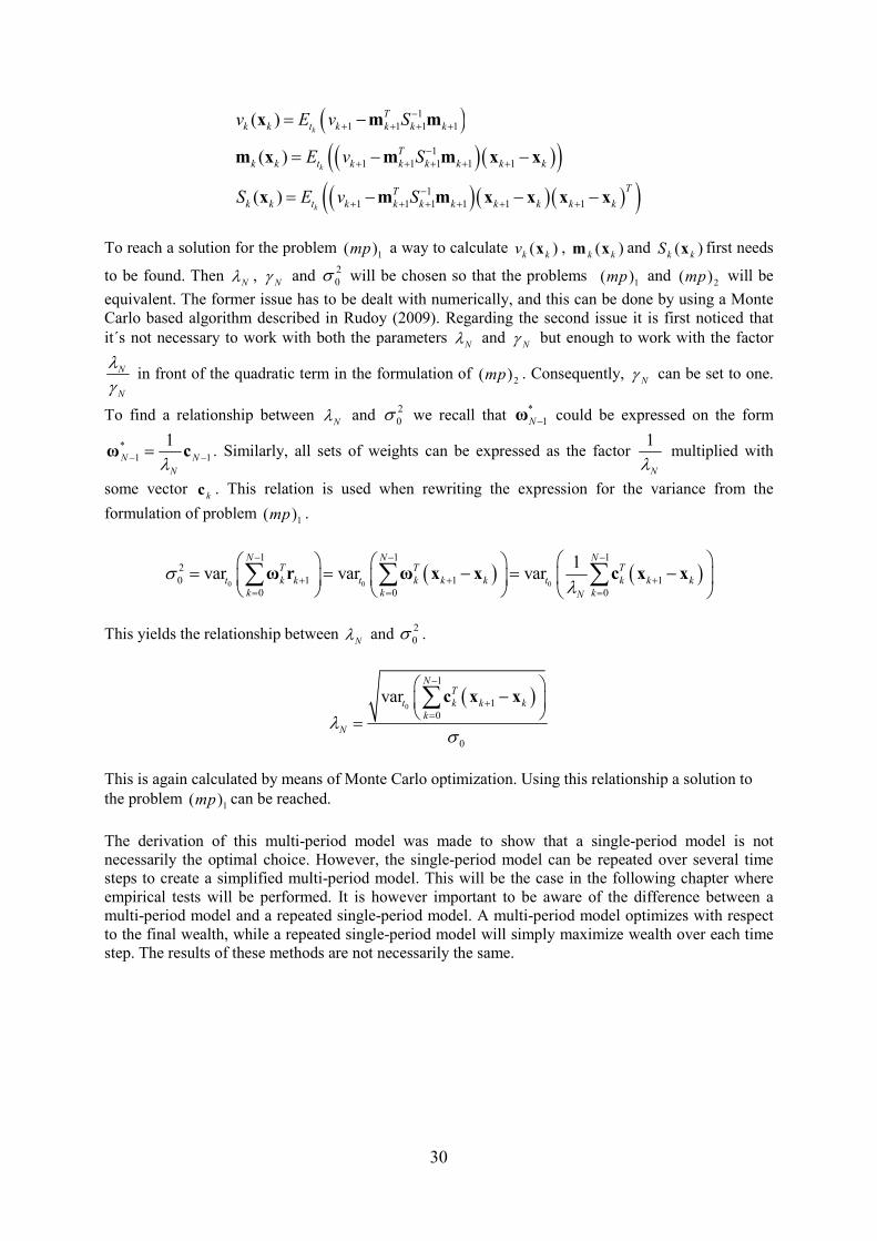
Figure 7. The outcome of the trading simulation. Surprisingly, the investor that weighted his assets equally was
best off. The mean-variance optimizer and the mean-LPM(2) optimizer followed each other closely.
Figure 8. This figure is a zoom of the mean-variance and mean-LPM(2) portfolio simulations from Figure 7.
Clearly it can be seen how mean-LPM(2) optimization leads to more volatile portfolio values.

34
Figure 7 shows that the investor that weighted his assets equally was best off. The other two, the optimizers, had similar returns over the period. However, the value of the mean-LPM(2) optimizer´s portfolio seems to fluctuate a bit more. A summary of more detailed results are shown in Table 1. Equally weighted portfolio Mean-variance portfolio Mean-LPM(2) portfolio
Return (daily) 0.031% 0.023% 0.023% Standard deviation
(on daily returns)
1.1% 1.5% 2.7%
LPM(2), [] 1.2 95.4 310.0
Table 1. Results of the trading simulation shown in Figure 7.
The weights of the two optimizing investors will also be analyzed in more detail. In Figure 9 the weights of the mean-variance optimizer can be seen. This figure clearly demonstrates one of the problems with mean-variance optimization, most of the time the money is put in one single asset, in this case in asset 2. The weights of the mean-LPM(2) investor is shown in Figure 10. Clearly the weights are less extreme in the sense that not all money is put in one or two of the assets. Looking at the results in Table 1 the mean-LPM(2) investor seems to hold a slightly riskier portfolio than the mean-variance investor. However, the fact that the mean-variance investor puts almost all his money in one asset is a big risk in itself which is not accounted for in the risk measures used.
Figure 9. The weights of the mean-variance investor during the trading period.
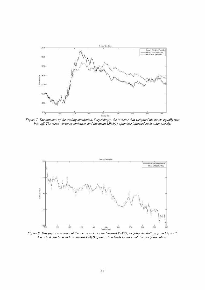
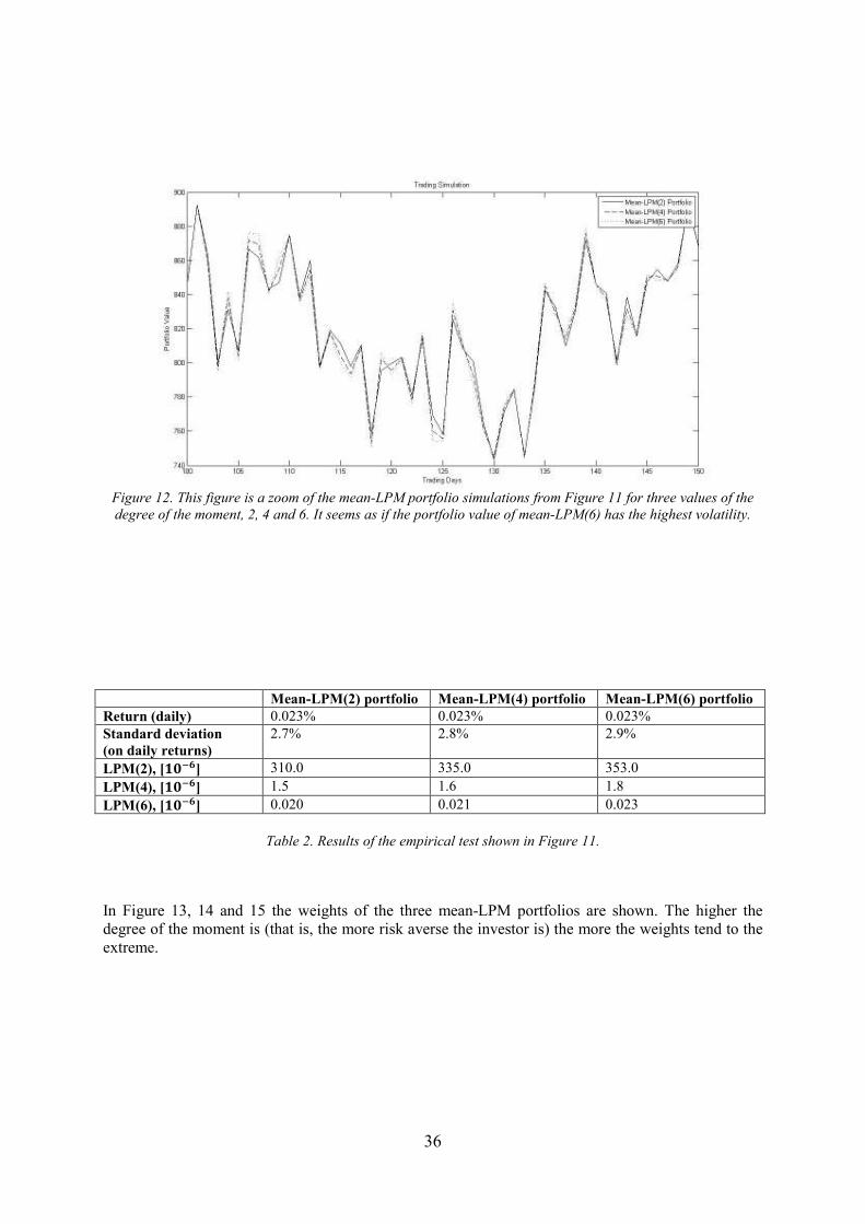
The empirical analysis is now extended to mean-LPM optimizing investors with varying risk aversion. For 2, 4 and 6 degrees of the moment the mean-LPM portfolios are shown in Figure 10. The differences between the portfolios are hardly seen, and Table 2 shows that the risk and return for the different portfolios differ only slightly.

35
Figure 10. The weights of the mean-LPM(2) investor during the trading period.
Figure 11. Mean-LPM portfolio values for three investors with different degree of the moment, 2, 4 and 6. There
is hardly any difference at all between the performances of the portfolios.
36
Figure 12. This figure is a zoom of the mean-LPM portfolio simulations from Figure 11 for three values of the
degree of the moment, 2, 4 and 6. It seems as if the portfolio value of mean-LPM(6) has the highest volatility.
Table 2. Results of the empirical test shown in Figure 11.
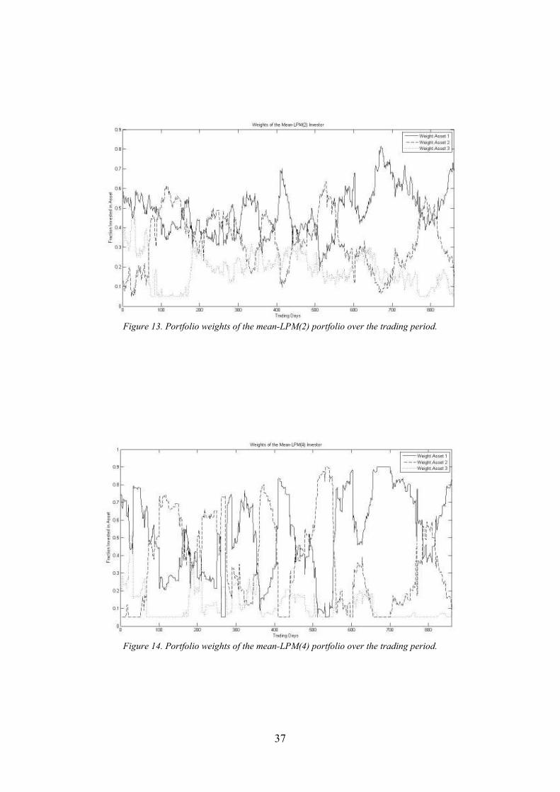
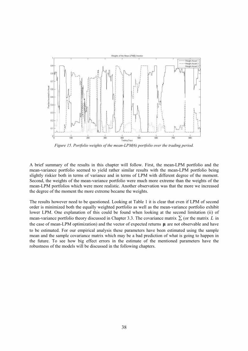
In Figure 13, 14 and 15 the weights of the three mean-LPM portfolios are shown. The higher the degree of the moment is (that is, the more risk averse the investor is) the more the weights tend to the extreme.
Mean-LPM(2) portfolio Mean-LPM(4) portfolio Mean-LPM(6) portfolio Return (daily) 0.023% 0.023% 0.023% Standard deviation
(on daily returns) 2.7% 2.8% 2.9%
LPM(2), [] 310.0 335.0 353.0 LPM(4), [] 1.5 1.6 1.8 LPM(6), [] 0.020 0.021 0.023
37
Figure 13. Portfolio weights of the mean-LPM(2) portfolio over the trading period.
Figure 14. Portfolio weights of the mean-LPM(4) portfolio over the trading period.
38
Figure 15. Portfolio weights of the mean-LPM(6) portfolio over the trading period.
A brief summary of the results in this chapter will follow. First, the mean-LPM portfolio and the mean-variance portfolio seemed to yield rather similar results with the mean-LPM portfolio being slightly riskier both in terms of variance and in terms of LPM with different degree of the moment. Second, the weights of the mean-variance portfolio were much more extreme than the weights of the mean-LPM portfolios which were more realistic. Another observation was that the more we increased the degree of the moment the more extreme became the weights.
The results however need to be questioned. Looking at Table 1 it is clear that even if LPM of second order is minimized both the equally weighted portfolio as well as the mean-variance portfolio exhibit lower LPM. One explanation of this could be found when looking at the second limitation (ii) of mean-variance portfolio theory discussed in Chapter 3.3. The covariance matrix ∑ (or the matrix L in the case of mean-LPM optimization) and the vector of expected returns µ are not observable and have to be estimated. For our empirical analysis these parameters have been estimated using the sample mean and the sample covariance matrix which may be a bad prediction of what is going to happen in the future. To see how big effect errors in the estimate of the mentioned parameters have the robustness of the models will be discussed in the following chapters.
39
Chapter 6
Robustness Analysis
Looking at the results from Chapter 5 two conclusions can be draw. First, mean-LPM optimization did not yield significantly better portfolios in terms of risk and return. Second, both mean-LPM and mean-variance optimization were clearly bad investment strategies compared to the equally weighted portfolio strategy. After the discussions in Chapter 2, 3 and 4 where the theory behind portfolio optimization was outlined this chapter will try to explain how it failed the empirical tests in the last chapter. Since the difference in terms of risk and return between mean-variance optimization and mean-LPM optimization was relatively small most of this chapter will discuss the robustness of mean-variance optimization. In Chapter 6.2 however both models will be compared and discussed.
6.1 Robustness
The de facto problem with mean-variance optimization that is known by practitioners and that occured in the last chapter is that all wealth is placed in a few assets and that the results (the efficient frontier and the portfolio weights) are sensitive to small changes in the estimated parameters µ and Σ . In fact,
Michaud (1989) goes as far as saying that mean-variance optimization is error-maximizing. “MV
optimization significantly overweighs those securities that have large estimated returns, negative
correlations and small variances. These securities are, of course, the ones most likely to have large
estimation errors”. This implies that if mean-variance optimization should yield good results the input parameters need to be estimated very accurately. In Chapters 6.3 and 6.4 two methods of doing this will be outlined. It is also important to mention that there is no clear-cut definition of robustness. Intuitively however, robustness is seen as the sensitivity of the output as a result of changes in the input. Optimally, small changes in the input parameters should yield small changes in the output parameters (the efficient frontier and the set of weights). To begin with however, a more general model of making portfolios more robust will be analyzed. The model was developed by König and Tüntücü (2004). They reformulate a more robust portfolio optimization problem by maximizing the worst-case scenario in the following way
40
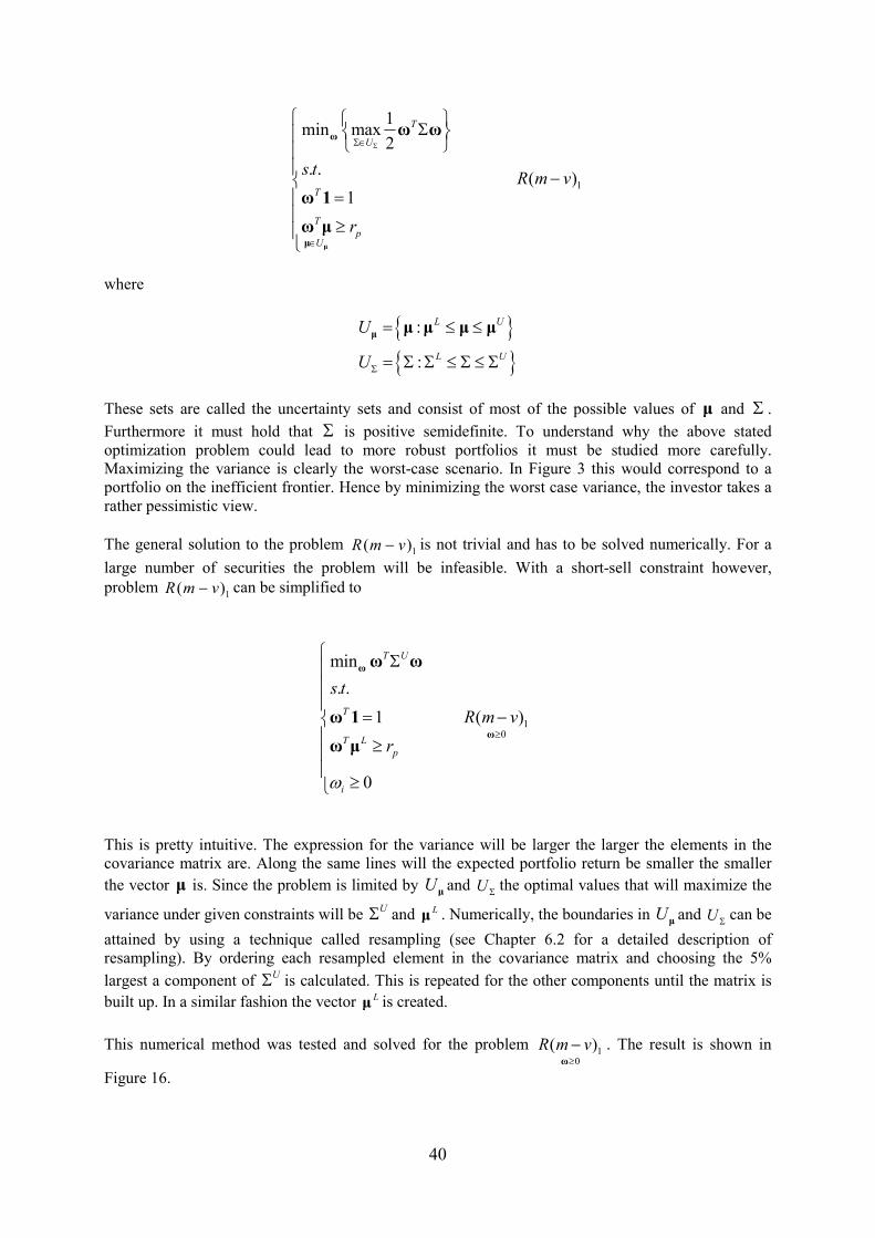
1
1min max
2
. . ( )1
T
U
T
T
pU
s tR m v
r
ΣΣ∈
∈
Σ
−
=
≥ µ
ω
µ
ω ω
ω 1
ω µ
where
:
:
L U
L U
U
UΣ
= ≤ ≤
= Σ Σ ≤ Σ ≤ Σ
µ µ µ µ µ
These sets are called the uncertainty sets and consist of most of the possible values of µ and Σ .
Furthermore it must hold that Σ is positive semidefinite. To understand why the above stated optimization problem could lead to more robust portfolios it must be studied more carefully. Maximizing the variance is clearly the worst-case scenario. In Figure 3 this would correspond to a portfolio on the inefficient frontier. Hence by minimizing the worst case variance, the investor takes a rather pessimistic view. The general solution to the problem 1( )R m v− is not trivial and has to be solved numerically. For a
large number of securities the problem will be infeasible. With a short-sell constraint however, problem 1( )R m v− can be simplified to
10
min
. .
1 ( )
0
T U
T
T L
p
i
s t
R m v
r
ω
≥
Σ
= − ≥
≥
ω
ω
ω ω
ω 1
ω µ
This is pretty intuitive. The expression for the variance will be larger the larger the elements in the covariance matrix are. Along the same lines will the expected portfolio return be smaller the smaller the vector µ is. Since the problem is limited by U
µand U Σ the optimal values that will maximize the
variance under given constraints will be UΣ and Lµ . Numerically, the boundaries in Uµand U Σ can be
attained by using a technique called resampling (see Chapter 6.2 for a detailed description of resampling). By ordering each resampled element in the covariance matrix and choosing the 5%
largest a component of UΣ is calculated. This is repeated for the other components until the matrix is built up. In a similar fashion the vector Lµ is created. This numerical method was tested and solved for the problem 1
0
( )R m v≥
−ω
. The result is shown in
Figure 16.
41
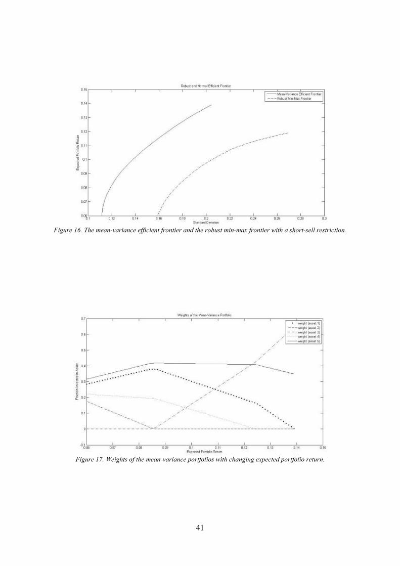
Figure 16. The mean-variance efficient frontier and the robust min-max frontier with a short-sell restriction.
Figure 17. Weights of the mean-variance portfolios with changing expected portfolio return.
42
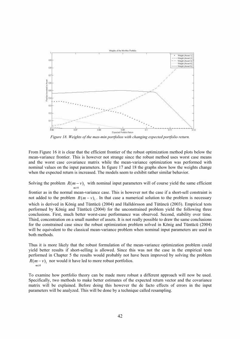
Figure 18. Weights of the max-min portfolios with changing expected portfolio return.
From Figure 16 it is clear that the efficient frontier of the robust optimization method plots below the mean-variance frontier. This is however not strange since the robust method uses worst case means and the worst case covariance matrix while the mean-variance optimization was performed with nominal values on the input parameters. In figure 17 and 18 the graphs show how the weights change when the expected return is increased. The models seem to exhibit rather similar behavior. Solving the problem 1
0
( )R m v≥
−ω
with nominal input parameters will of course yield the same efficient
frontier as in the normal mean-variance case. This is however not the case if a short-sell constraint is not added to the problem 1( )R m v− . In that case a numerical solution to the problem is necessary
which is derived in König and Tüntücü (2004) and Halldórsson and Tütüncü (2003). Empirical tests performed by König and Tüntücü (2004) for the unconstrained problem yield the following three conclusions. First, much better worst-case performance was observed. Second, stability over time. Third, concentration on a small number of assets. It is not really possible to draw the same conclusions for the constrained case since the robust optimization problem solved in König and Tüntücü (2004) will be equivalent to the classical mean-variance problem when nominal input parameters are used in both methods. Thus it is more likely that the robust formulation of the mean-variance optimization problem could yield better results if short-selling is allowed. Since this was not the case in the empirical tests performed in Chapter 5 the results would probably not have been improved by solving the problem
10
( )R m v≥
−ω
nor would it have led to more robust portfolios.
To examine how portfolio theory can be made more robust a different approach will now be used. Specifically, two methods to make better estimates of the expected return vector and the covariance matrix will be explained. Before doing this however the de facto effects of errors in the input parameters will be analyzed. This will be done by a technique called resampling.

43
6.2 Resampling
In this chapter the effects of estimation errors when using the sample mean and the sample covariance matrix will be discussed. This will be done by using a technique called resampling. Basically the method can be thought of as small errors being added to the “true” parameters. The effect of these added errors will thereafter be analyzed first by looking at the effect on the efficient frontiers and second by looking at the effect on the portfolio weights. This analysis will be performed to realize how estimation errors in Chapter 5 may have affected the results. The method will now be explained in more detail. By using resampling it can graphically be shown how the estimation errors in µ and ∑ affects the efficient frontier. Resampling works the following way. Assume that the input parameters have been estimated using T observations from m securities resulting in a T m× matrix consisting of the data.
This yields the parameters *0µ and
*0∑ . Next, a new T m× matrix is created by randomly drawing one
row at the time from the original matrix until the whole matrix has been filled with data (one row can
be drawn many times). The parameters are thereafter estimated again, resulting in *1µ and
*1∑ . This
process is repeated n times. For each of the estimated pairs of parameters optimal weights are
calculated. When plotting the efficient frontiers however, *0µ and
*0∑ are used. Since the optimized
weights are not optimal for *0µ and
*0∑ all the resampled frontiers will plot below the original frontier.
Resampling is thus used as a way of observing the effects of errors in the parameter estimates. The data used consists of the daily closing prices of the indices used for the empirical tests in Chapter 5.2. The last 150 trading days have been used which is a realistic number if we want to make sure that the data is still relevant. In Figure 20 the resampled efficient frontiers of the mean-variance investor are shown. Small errors in the parameters seem to shift the efficient frontier rather much. The following tests will all be made with a short-sell constraint. This is crucial for the results. Allowing short-selling yields resampled frontiers that can be seen in Figure 19. It is clear that a short-sell constraint has a strong influence on the portfolios. It is however hard to make comparations with mean-LPM efficient frontiers based on these kinds of plots. To deal with this a technique developed by Michaud (1998) called resampled efficiency will be used. This method calculates an average of all the resampled efficient frontiers based on their weights. Thus the average set of weights that will constitute the portfolio number m along the average resampled efficient frontier is expressed as
,1
1 nresampled
m i m
in =
= ∑ω ω
where n is the number of resampled frontiers and ,i mω is the portfolio number m along one of the
resampled frontiers. Using this relation an average resampled efficient frontier can be traced out. This will then plot below the original efficient frontier. The result of this when applied to Figure 20 can be seen in Figure 21. To make it comparable with the following plots the length scale on the vertical axis is of the same size in Figure 21, 23, 25 and 27. The procedure is repeated for the mean-LPM efficient frontiers with 2, 3 and 4 degrees of freedom respectively. The results are shown in Figure 22-27. For clarity the original efficient frontier has been marked with stars in Figure 20, 22, 24 and 26. The distance between the original efficient frontier and the average resampled efficient frontier is a sign of robustness. The smaller the distance, the less sensitive the frontier is for changes in the input data and the more robust the method is.
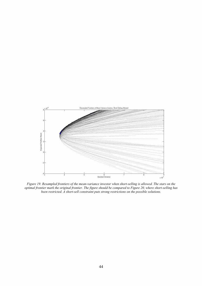
44
F
Figure 19. Resampled frontiers of the mean-variance investor when short-selling is allowed. The stars on the
optimal frontier mark the original frontier. The figure should be compared to Figure 20, where short-selling has
been restricted. A short-sell constraint puts strong restrictions on the possible solutions.
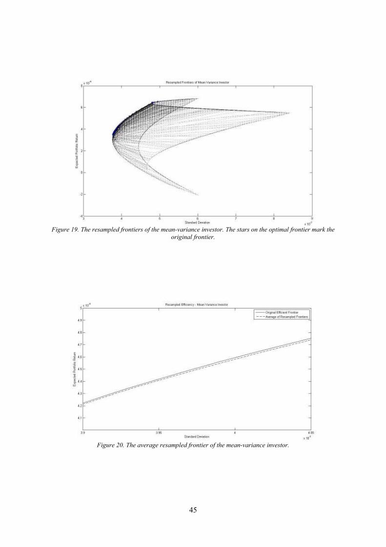
45
Figure 19. The resampled frontiers of the mean-variance investor. The stars on the optimal frontier mark the
original frontier.
Figure 20. The average resampled frontier of the mean-variance investor.
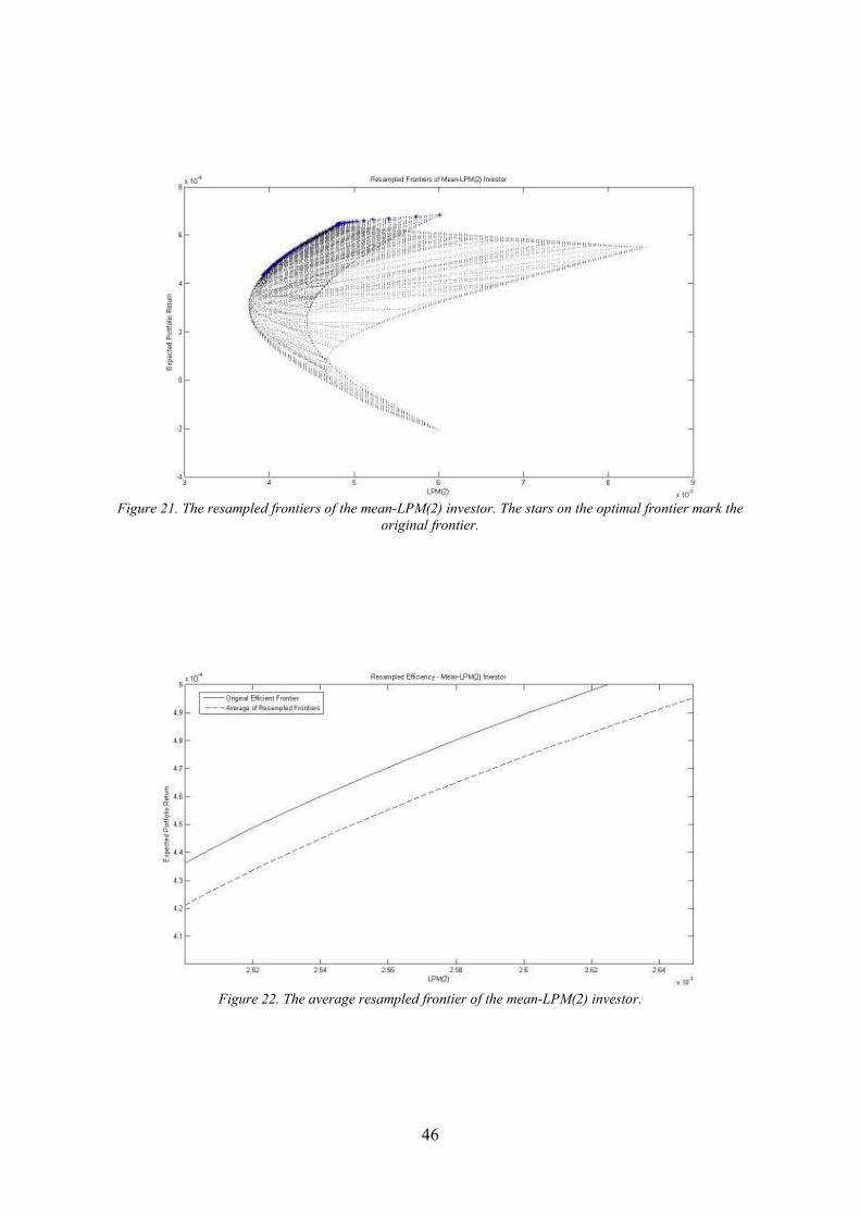
46
Figure 21. The resampled frontiers of the mean-LPM(2) investor. The stars on the optimal frontier mark the
original frontier.
Figure 22. The average resampled frontier of the mean-LPM(2) investor.
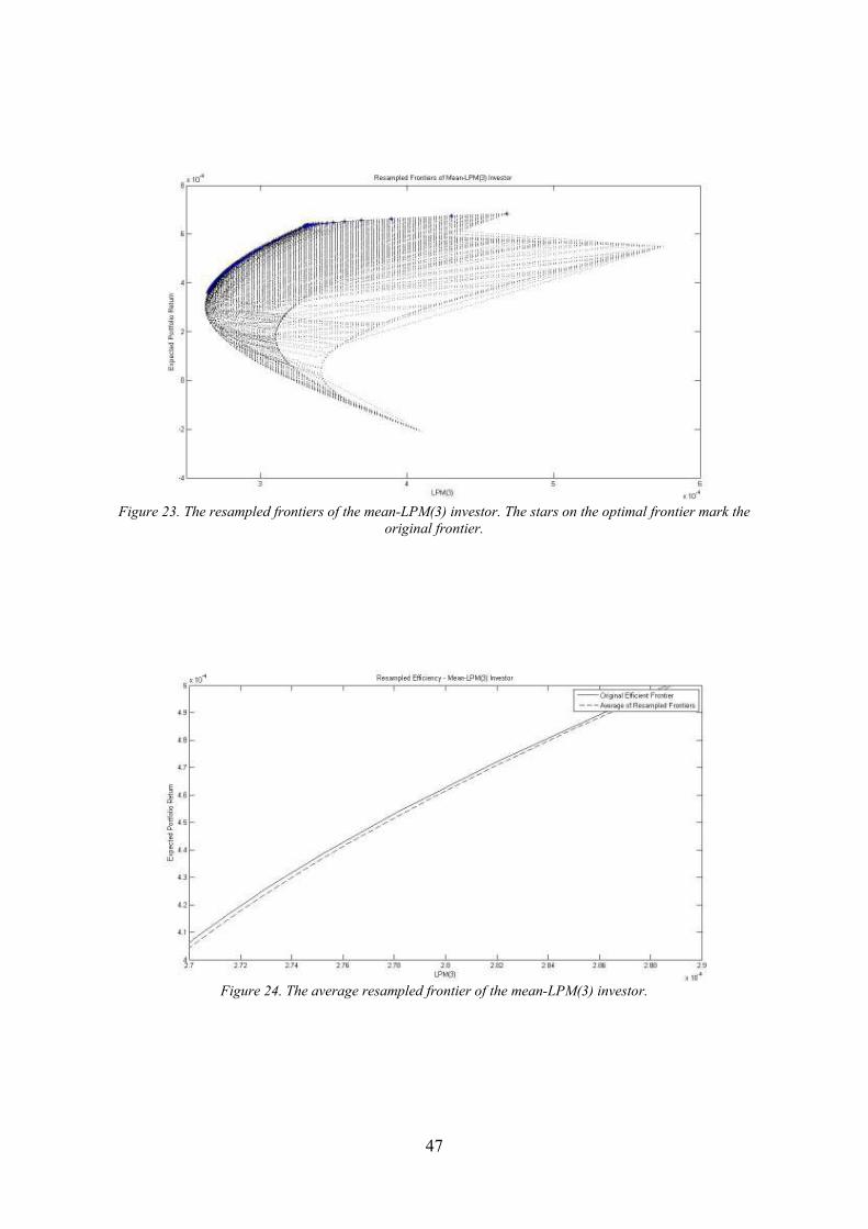
47
Figure 23. The resampled frontiers of the mean-LPM(3) investor. The stars on the optimal frontier mark the
original frontier.
Figure 24. The average resampled frontier of the mean-LPM(3) investor.
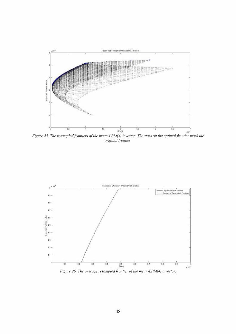
48
Figure 25. The resampled frontiers of the mean-LPM(4) investor. The stars on the optimal frontier mark the
original frontier.
Figure 26. The average resampled frontier of the mean-LPM(4) investor.

49
Looking at Figure 20, 22, 24 and 26 it seems as if the higher the degree of the moment the more robust the optimization method will be. The distance between the original efficient frontier and the resampled efficient frontier seems to get smaller each time the degree of the moment is increased. Mean-variance optimization seems to have the same robustness as mean-LPM optimization with a degree of the moment somewhere between 3 and 4. However, since the risk measures are different we should be a bit careful before drawing too general conclusions of the robustness tests performed above.
Another way of trying to capture how the estimation error affects portfolios is by looking at how the weights change for the resampled portfolios. The result can be seen in Figure 27. What is interesting to notice in the figure is the variance of the weights. Optimally small changes in the parameters should give rise to small changes in the weights. Looking at Figure 27 this is however not the case. The variance of the weights from Figure 27 are summarized in Table 3 below.
Figure 27. Distributions of the weights of the mean-variance investor and the mean-LPM investor with 2, 3 and
4 degrees of the moment.
Weight 1 Weight 2 Weight 3
Variance
Mean-Variance 0.0454 0.0270 0.0307 Mean-LPM(2) 0.0793 0.0462 0.0822 Mean-LPM(3) 0.0418 0.0229 0.0283 Mean-LPM(4) 0.0136 0.0094 0.0106
Table 3. Variance of the weights when the different models were tested using resampling.
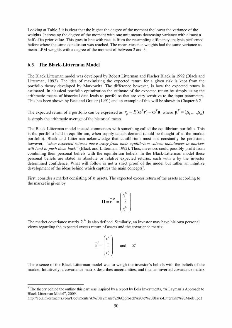
50
Looking at Table 3 it is clear that the higher the degree of the moment the lower the variance of the weights. Increasing the degree of the moment with one unit means decreasing variance with almost a half of its prior value. This goes in line with results from the resampling efficiency analysis performed before where the same conclusion was reached. The mean-variance weights had the same variance as mean-LPM weights with a degree of the moment of between 2 and 3.
6.3 The Black-Litterman Model
The Black Litterman model was developed by Robert Litterman and Fischer Black in 1992 (Black and Litterman, 1992). The idea of maximizing the expected return for a given risk is kept from the portfolio theory developed by Markowitz. The difference however, is how the expected return is estimated. In classical portfolio optimization the estimate of the expected return by simply using the arithmetic means of historical data leads to portfolios that are very sensitive to the input parameters. This has been shown by Best and Grauer (1991) and an example of this will be shown in Chapter 6.2.
The expected return of a portfolio can be expressed as ( )T T
pr E= =ω r ω µ where 1( ,..., )T
nµ µ=µ
is simply the arithmetic average of the historical mean. The Black-Litterman model instead commences with something called the equilibrium portfolio. This is the portfolio held in equilibrium, when supply equals demand (could be thought of as the market portfolio). Black and Litterman acknowledge that equilibrium must not constantly be persistent, however, “when expected returns move away from their equilibrium values, imbalances in markets
will tend to push them back” (Black and Litterman, 1992). Thus, investors could possibly profit from combining their personal beliefs with the equilibrium beliefs. In the Black-Litterman model these personal beliefs are stated as absolute or relative expected returns, each with a by the investor determined confidence. What will follow is not a strict proof of the model but rather an intuitive development of the ideas behind which captures the main concepts4. First, consider a market consisting of n assets. The expected excess return of the assets according to the market is given by
1M
M
M
n
r
r
= =
Π r M
The market covariance matrix MΣ is also defined. Similarly, an investor may have his own personal views regarding the expected excess return of assets and the covariance matrix.
1I
I
I
n
r
r
=
r M and IΣ
The essence of the Black-Litterman model was to weigh the investor´s beliefs with the beliefs of the market. Intuitively, a covariance matrix describes uncertainties, and thus an inverted covariance matrix
4 The theory behind the outline this part was inspired by a report by Eola Investments, “A Layman´s Approach to Black Litterman Model”, 2009. http://eolainvestments.com/Documents/A%20laymans%20Approach%20to%20Black-Litterman%20Model.pdf
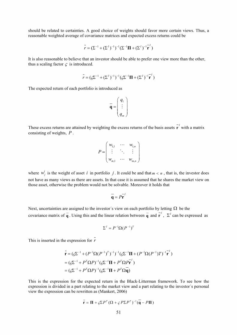
51
should be related to certainties. A good choice of weights should favor more certain views. Thus, a reasonable weighted average of covariance matrices and expected excess returns could be
1 1 1 1 1( ( ) ) ( ( ) )II Ir − − − − −= Σ + Σ Σ + ΣΠ r%
It is also reasonable to believe that an investor should be able to prefer one view more than the other, thus a scaling factor ς is introduced.
1 1 1 1 1( ( ) ) ( ( ) )
II Ir ς ς− − − − −= Σ + Σ Σ + ΣΠ r% The expected return of each portfolio is introduced as
1
m
q
q
=
q M
These excess returns are attained by weighting the excess returns of the basis assets I
r with a matrix consisting of weights, P .
1,1 1,
,1 ,
n
m m n
w w
P
w w
=
L
M O M
L
where i
jw is the weight of asset i in portfolio j . It could be and thatm n< , that is, the investor does
not have as many views as there are assets. In that case it is assumed that he shares the market view on those asset, otherwise the problem would not be solvable. Moreover it holds that
I
P=q r
Next, uncertainties are assigned to the investor´s view on each portfolio by letting Ω be the
covariance matrix of q . Using this and the linear relation between q and I
r , IΣ can be expressed as
1 1( )I TP P− −Σ = Ω
This is inserted in the expression for r%
1 1 1 1 1 1 1 1 1
1 1 1
1 1 1
( ( ( ) ) ) ( ( ( ) ) )
( ) ( )
( ) ( )
IT
IT T
T T
P P P P T
P P P P
P P P
ς ς
ς ς
ς ς
− − − − − − − − −
− − −
− − −
= Σ + Ω Σ + Ω
= Σ + Ω Σ + Ω
= Σ + Ω Σ + Ω
r Π r
Π r
Π q
%
This is the expression for the expected return in the Black-Litterman framework. To see how the expression is divided in a part relating to the market view and a part relating to the investor´s personal view the expression can be rewritten as (Mankert, 2006)
1( ) ( )T TP P P Pς ς −= + Σ Ω + Σ −r Π q Π%

52
Written on this form it is clear that the first part expresses the views of the market while the second
part expresses the views of the investor. Recall for example the relation I
P=q r . If the views of the investor equals the views of the market (which happened if the investor didn´t have any personal
views at all) then I
=r Π and thus P=q Π and the expected return will equal the expected return according to the market view.
To get a better understanding of the Black-Litterman model a numerical example will be discussed. Assume that the data is the same as in Chapter 6.2. Our personal views about the three assets need to be specified. Suppose that we believe that asset 1 will outperform asset 3 with 1% on a yearly basis. Furthermore, assume that we think that asset 2 will have an excess return of 2% on a yearly basis.
Since the universe of assets only consists of three assets, the matrix P and the vector q that
summarize our views about the market are given by
1 0 1
0 1 0P
− =
1%
2%
=
q
Π is the mean of historical returns and Σ is the well known sample covariance matrix. The parameter ς is often calculated as the ratio between the number of views (two in this example) and the number
of assets (three in this example) (Mankert, 2006). Thus, 2
3
n
mς = = . The matrix Ω associates risk
with our personal views about the market. Ω is assumed to be diagonal, that is, the correlation between views are zero. He and Litterman (1999) express Ω as
( ( ) )Tdiag P PςΩ = Σ
assuming that the variance of our views will be proportional to the variance of the asset returns. The input parameters to the Black-Litterman model are now determined and the efficient frontier can now be plotted. The result can be seen in Figure 28 and to have something to compare with the efficient frontier when the sample mean was used as input parameter is plotted as well. Clearly, our personal views mattered quite a lot since the frontiers in Figure 28 look pretty different. Subsequently the same robustness tests as in the last chapter was performed. First resampling was used to create 1000 frontiers (Figure 29 and 31) and then the theory behind resampled efficiency was used to find an average of the resampled frontiers (Figure 30 and 32).
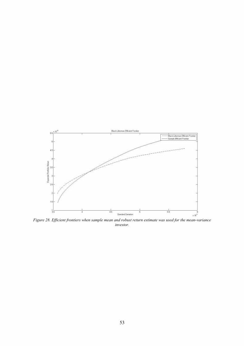
53
Figure 28. Efficient frontiers when sample mean and robust return estimate was used for the mean-variance
investor.
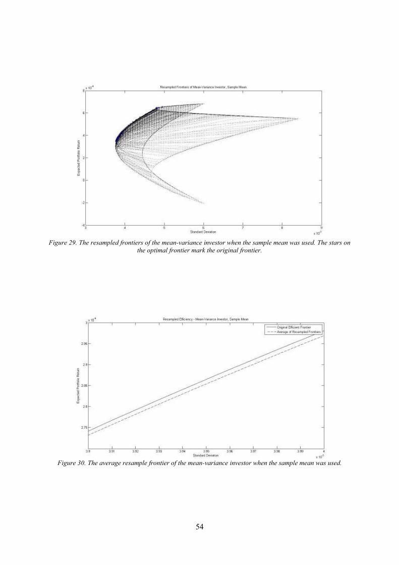
54
Figure 29. The resampled frontiers of the mean-variance investor when the sample mean was used. The stars on
the optimal frontier mark the original frontier.
Figure 30. The average resample frontier of the mean-variance investor when the sample mean was used.

55
Figure 31. The resampled frontiers of the mean-variance investor when the Black-Litterman mean was used. The
stars on the optimal frontier mark the original frontier.
Figure 32. The average resampled frontier of the mean-variance investor when the Black-Litterman mean was
used.
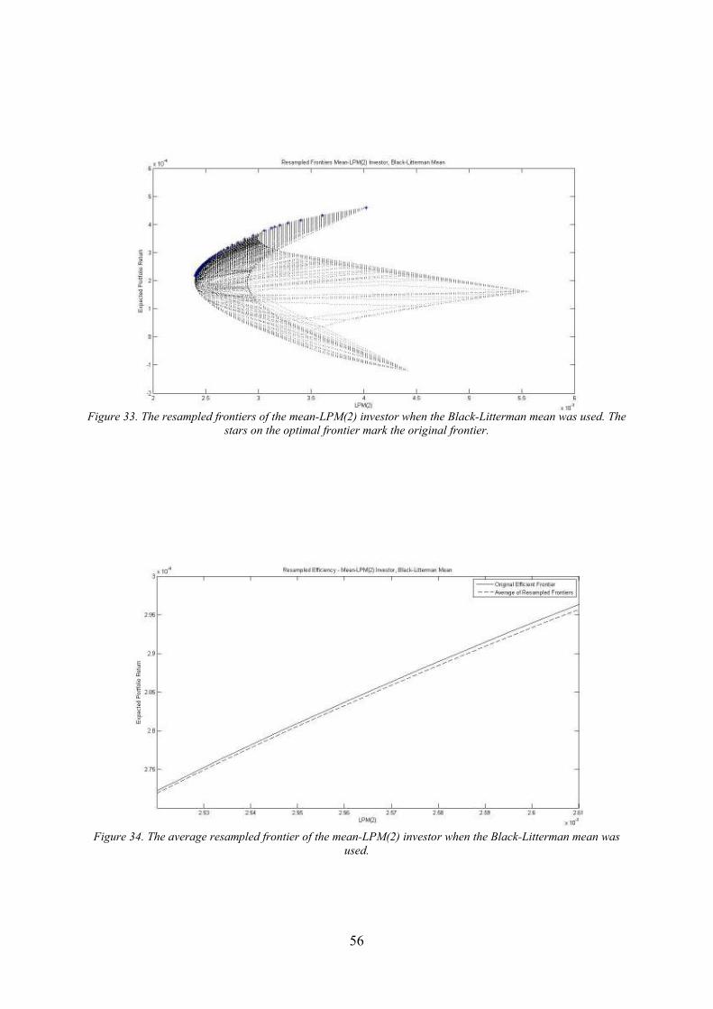
56
Figure 33. The resampled frontiers of the mean-LPM(2) investor when the Black-Litterman mean was used. The
stars on the optimal frontier mark the original frontier.
Figure 34. The average resampled frontier of the mean-LPM(2) investor when the Black-Litterman mean was
used.
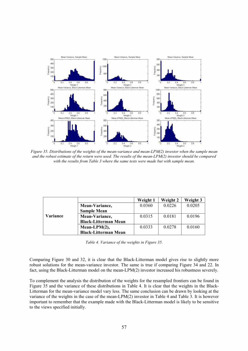
57
Figure 35. Distributions of the weights of the mean-variance and mean-LPM(2) investor when the sample mean
and the robust estimate of the return were used. The results of the mean-LPM(2) investor should be compared
with the results from Table 3 where the same tests were made but with sample mean.
Variance
Weight 1 Weight 2 Weight 3
Mean-Variance,
Sample Mean
0.0360 0.0226 0.0205
Mean-Variance,
Black-Litterman Mean
0.0315 0.0181 0.0196
Mean-LPM(2),
Black-Litterman Mean
0.0333 0.0278 0.0160
Table 4. Variance of the weights in Figure 35.
Comparing Figure 30 and 32, it is clear that the Black-Litterman model gives rise to slightly more robust solutions for the mean-variance investor. The same is true if comparing Figure 34 and 22. In fact, using the Black-Litterman model on the mean-LPM(2) investor increased his robustness severely. To complement the analysis the distribution of the weights for the resampled frontiers can be found in Figure 35 and the variance of these distributions in Table 4. It is clear that the weights in the Black-Litterman for the mean-variance model vary less. The same conclusion can be drawn by looking at the variance of the weights in the case of the mean-LPM(2) investor in Table 4 and Table 3. It is however important to remember that the example made with the Black-Litterman model is likely to be sensitive to the views specified initially.
58
6.4 Shrinkage Estimation of the Covariance Matrix
Even if it was empirically shown by Chopra and Ziemba (1993) that errors in risk estimates are less significant than errors in return estimates the estimation of covariance matrices is still significant and important to be aware off. In practice, fund managers often end up with a larger number of assets than data observations and this will make estimation errors significant. In classical portfolio optimization the sample covariance estimator is used. An element of the sample covariance matrix is estimated according to
*, , ,
1
1( )( )
1
NT
i ji j i k j k
k
x x x xN =
Σ = − −− ∑
where N is the number of historical observations. It has been shown by Jobson and Korkie (1980) that the sample estimator is biased with considerable estimation errors when the number of assets is large and the number of observations is small. Since this scenario is often present when using financial data, methods to better estimate the covariance matrix have been developed. An estimation method developed by Ledoit and Wolf (2003) will now be discussed. Before going through the details of their estimation method the ideas behind Sharpe´s (1963) single index model will be developed. This is one of the simplest models to characterize asset returns where the returns only depend on one factor, usually a market index
mf .
i i i m ir fα β ε= + + for 1,...,i N=
( , )
( )i m
i
m
cov r r
var rβ =
Where
mr is the market return and iα is a constant. Moreover the following assumptions hold
2
2
( ) 0
( )
( , ) 0
( , ) 0
( )
i
m
i
i
i j
i m
m f
E
var
cov for i j
cov f
var f
ε
ε
ε σ
ε ε
ε
σ
=
=
= ≠
=
=
The covariance matrix of the asset returns can then be expressed as
2
m
T
f εσΦ = +Σββ
Where εΣ is the covariance matrix of
iε . The estimated version of Φ is expressed as
* 2* * * *
m
T
fF εσ= +Σβ β
The reason why the single index model was explained is because in the article by Ledoit and Wolf the estimated covariance matrix is a weighted average of the covariance matrix F and the sample
covariance matrix *Σ
59
The tricky part is to chose α optimally. The solution is found by minimizing the distance L between
the estimated covariance matrix *Ψ and the true covariance matrix Σ.
2* *( ) (1 )L Fα α α= + − Σ − Σ
The calculations are not hard but tedious so we turn directly to the answer,
( )
* * *, , ,
1 1*
2* * *, , , ,
1 1
Var( ) Cov( , )
Var( )
N N
i j i j i j
i j
N N
i j i j i j i j
i j
F
F
α = =
= =
Σ − Σ
=
−Σ + Ψ −Σ
∑∑
∑∑
According to Theorem 1 in Ledoit and Wolf (2003) *α can be expressed as
*2
1 1
T T
π ρα
γ−
= + Ο
Where T is the number of assets and ρ , π and γ can be expressed as
,1 1
N N
i j
i j
π π= =
=∑∑ with ( )*, ,AsyVari j i jTπ = Σ
( )*AsyVar t is an abbreviation for the asymptotic variance of the estimator *t and is basically the
variance of the estimator *t when the number of observation the estimate is based on tends to infinity.
The same holds for ( )* *AsyCov ,b t where *b and *t are arbitrary estimators which will be used
below.
,1 1
N N
i j
i j
ρ ρ= =
=∑∑ with ( )* *, , ,AsyCov ,i j i j i jT F Tρ = Σ
,1 1
N N
i j
i j
γ γ= =
=∑∑ with ( )2*, , ,i j i j i jγ = Ψ −Σ
By using π ρ
κγ−
=
the asymptotically optimal shrinkage estimator can be expressed as
* *(1 )FT T
κ κ+ − Σ
To reach an estimation of κ the parameters ρ , π and γ first need to be estimated. In Ledoit and Wolf
(2003) these are given by
* * *(1 )Fα αΨ = + − Σ

60
( )( )( )2* *. ., , , ,
1
1 T
i ji j i t j t i j
t
x x x xT
π=
= − − −Σ∑
*,
*, *
, ,1
1
i j
Ti j
i j t
t
for i j
for i jT
π
ρρ
=
=
= ≠
∑
If *,j mΣ is the covariance of the return of asset j with the return of the market and mx the average return
of the market then
* * * * * *, , , , , , , , ,* *
, , , , , , ,*2,
( ) ( ) ( )( )( )( )
i j mj m m m i t i m m m j t i m j m m tm i ji j t m t i t j t i j i j
m m
x x x x x xx x x x x x Fρ
Σ Σ − +Σ Σ − −Σ Σ −= − − − − Σ
Σ
And finally
( )2* *, , ,i j i j i jFγ = −Σ
The derivation of the robust estimate of the covariance matrix according to Ledoit and Wolf (2003) was not trivial. To get a better sense of how their estimate performs versus the sample covariance matrix it will numerically be tested on the same set of data that was used in Chapter 6.2. In these examples the mean-LPM investor will not be considered since the estimation technique developed by Ledoit and Wolf (2003) was specifically made for the covariance matrix. In Figure 36 the efficient frontier when using the robust estimate of the covariance matrix plots below the efficient frontier drawn when using the sample estimate of the covariance matrix.
Figure 36. The efficient frontiers of the mean-variance investor when the sample estimate of the covariance
matrix was used compared with when the robust estimate of the covariance matrix was used.

61
Figure 37. The resampled frontiers of the mean-variance investor when using the sample covariance matrix. The
stars on the optimal frontier mark the original frontier.
Figure 38. The average of resampled frontiers of the mean-variance investor when using the sample covariance
matrix.
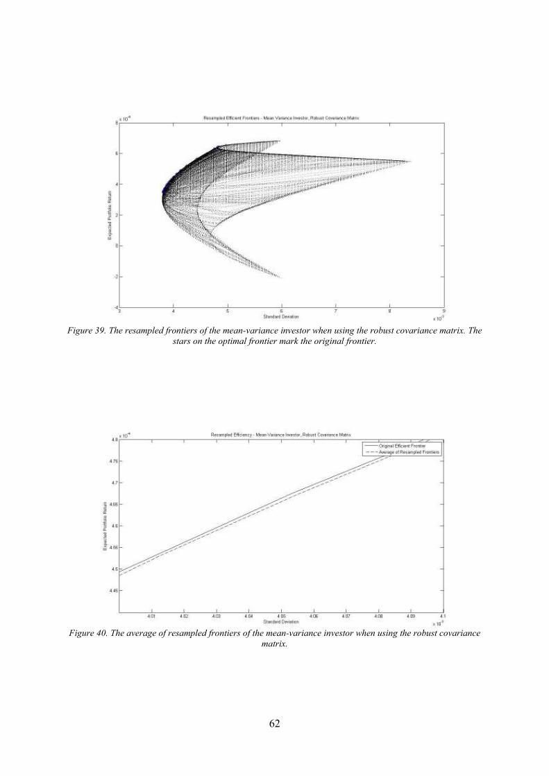
62
Figure 39. The resampled frontiers of the mean-variance investor when using the robust covariance matrix. The
stars on the optimal frontier mark the original frontier.
Figure 40. The average of resampled frontiers of the mean-variance investor when using the robust covariance
matrix.
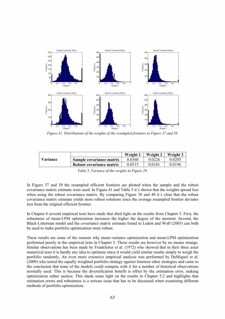
63
Figure 41. Distributions of the weights of the resampled frontiers in Figure 37 and 39.
Table 5. Variance of the weights in Figure 29.
In Figure 37 and 39 the resampled efficient frontiers are plotted when the sample and the robust covariance matrix estimate were used. In Figure 41 and Table 5 it´s shown that the weights spread less when using the robust covariance matrix. By comparing Figure 38 and 40 it´s clear that the robust covariance matrix estimate yields more robust solutions since the average resampled frontier deviates less from the original efficient frontier. In Chapter 6 several empirical tests have made that shed light on the results from Chapter 5. First, the robustness of mean-LPM optimization increases the higher the degree of the moment. Second, the Black-Litterman model and the covariance matrix estimate found in Ledoit and Wolf (2003) can both be used to make portfolio optimization more robust. These results are some of the reasons why mean-variance optimization and mean-LPM optimization performed poorly in the empirical tests in Chapter 5. These results are however by no means strange. Similar observations has been made by Frankfurter et al. (1972) who showed that in their three asset numerical tests it is hardly any idea to optimize since it would yield similar results simply to weigh the portfolio randomly. An even more extensive empirical analysis was performed by DeMiguel et al. (2009) who tested the equally weighted portfolio strategy against fourteen other strategies and came to the conclusion that none of the models could compete with it for a number of historical observations normally used. This is because the diversification benefit is offset by the estimation error, making optimization rather useless. This sheds some light on the results in Chapter 5.2 and highlights that estimation errors and robustness is a serious issue that has to be discussed when examining different methods of portfolio optimization.
Variance
Weight 1 Weight 2 Weight 3
Sample covariance matrix 0.0360 0.0226 0.0205 Robust covariance matrix 0.0315 0.0181 0.0196
64
Chapter 7
Conclusions
7.1 Conclusions
In this thesis the mean-variance optimization problem was first discussed. This model was extended to mean-LPM portfolio optimization which had some theoretically favorable features which mean-variance optimization lacked. The models were empirically tested and they had a similar performance in terms of risk and return, the mean-LPM model however being slightly riskier. They were both outperformed by an equally weighted portfolio strategy. This raised a serious question whether the optimization methods were reliable. A robustness analysis was performed to provide some answers and to examine whether the models could be affected severely by estimation errors. The following conclusions were drawn. Even if mean-LPM optimization has some superior features over mean-variance optimization the models yield similar returns while mean-LPM optimization was slightly riskier in terms of standard deviation and LPM of degree 2, 4 and 6. Mean-LPM optimization did have the desirable feature of avoiding extreme allocations. This was not the case for mean-variance allocation, where all wealth was put in one asset over almost the whole trading period. Both optimization methods performed worse than the equally weighted portfolio and they were also riskier in terms of the same risk measures as mentioned above. A robustness analysis showed that the higher the degree of the moment the more robust were the mean-LPM optimization. One method of estimating the expected return was tested and results showed that the portfolios were indeed more robust both for mean-variance and for mean-LPM(2) investors. The same tests were performed on a method for estimating covariance matrices, again with the result that resulting mean-variance portfolios were more robust. In summary, mean-LPM optimization does provide the investor with some beneficial features. However, both mean-LPM and mean-variance optimization are sensitive to estimation errors. The robustness of the methods can indeed be improved by using modern estimation techniques. However, in our tests the optimization methods yielded so bad results that the question whether it is worthwhile to optimize remains open.

65
7.2 Future Analysis
For future improvements of the results in this thesis to be made several different topics could be developed further. The analysis could be extended to include more assets to examine whether this affects the performance of the models. The methods could in addition be tested on more periods of different time scales. An interesting topic could also be to examine different multi-period models and see whether they would outperform the single-period model used in this thesis. The more robust estimation techniques could be used in the back-testing simulation which would possibly show their real strengths. With that said, there are many interesting topics that could be developed further.
66
References
1. Artzner, P., Delbaen, F., Eber, J., Heath, D., (1999), “Coherent Measures of Risk”, Mathematical Finance, v9, n3 (July), 203-28.
2. Acerbi, C., Tasche, D., (2001), “Expected Shortfall: a natural coherent alternative to Value at
Risk”, Economic Notes, Volume 31.
3. Bachelier, L., (1900), “Théorie de la Spéculation”, Annales Scientifiques de l’École Normale Supérieure, 3 (18), 143–210.
4. Bawa, V. S., (1975), “Optimal Rules for Ordering Uncertain Prospects”, Journal of Financial Economics, 2, 95-121.
5. Black, F., Litterman, R., (1992), “Global Portfolio Optimization”, Financial Analysts Journal, September pp. 28-43.
6. Best, M. J., Grauer, R. R., (1991), “On the Sensitivity of Mean-Variance-Efficient Portfolios to
Changes in Asset Means: Some Analytical and Computational Results”, The Review of Financial Studies, Vol. 4, No. 2, pp. 315-342.
7. Chopra, V. K., Ziemba, W. T., (1993), “The Effects of Errors in Means, Variances and
Covariances on Optimal Portfolio Choice”, Journal of Portfolio Management, v19(2), 6-12. 8. Cumova, D., Moreno, D., Nawrocki, D., (2006), “The Critical Line Algorithm for UPM-LPM
Parametric General Asset Allocation Problem With Allocation Boundaries and Linear
Constraints”, London UK: Palgrave Macmillan: Risk and Portfolio Management: The New Frontier. 9. DeMiguel, V., Garlappi, L., Uppal, R., (2009), ”Optimal Versus Naïve Diversification: How
Inefficient is the 1/N Portfolio Strategy?”, Review of Financial Studies, 22(5), 1915-1953. 10. Fishburn, P-C., (1977), “Mean Risk Analysis with Below Target Returns”, The American
Economic Review. 11. Frankfurter, G. M., Phillips, H. E., Seagle, J. P., (1971), “Portfolio Selection: The Effects of
Uncertain Means, Variances and Covariances”, Journal of Finance and Quantitative Analysis, 6, 1252-1262.

67
12. Föllmer, H., Schied, A., (2002), “Convex measures of risk and trading constraints”, Finance Stochast. 6, 429-447. 13. Halldórsson, B. V., Tütüncü, R. H., (2003), “An Interior-Point Method for a Class of Saddle-
Point Problems”, Journal of Optimization Theory and Applications 116(3), 559–590. 14. He, G., Litterman, R., (1999), “The Intuition Behind Black-Litterman Model Portfolios”,
Goldman Sachs Asset Management, Working paper. 15. Hogan,W. W., Warren, J.M., (1972), "Computation of the Efficient Boundary in the E-S Portfolio
Selection Model", Journal of Financial and Quantitative Analysis, 7, 1881-96. 16. Jarrow, R., Zhao, F., 2006, “Downside Loss Aversion and Portfolio Management”, Management
Science, volume 52, issue 4, April. 17. König, M., Tüntücü, R. H., (2004), ”Robust Asset Allocation”, Annals of Operations Research,
132, 132-157. 18. Li, D., Ng, W., (2000), “Optimal Dynamic Portfolio Selection: Multiperiod Mean-Variance
Formulation”, Mathematical Finance, 10(3):387-406. 19. Ledoit, O., Wolf, M., (2003), “Improved Estimation of the Covariance Matrix of Stock Returns”
Journal of Empirical Finance , 10 (5), 603-621.
20. Mankert, C., (2006), “The Black Litterman Model: mathematical and behavioral finance
approaches towards its use in practice”, Licentiate Thesis, Royal Institute of Technology, Stockholm.
21. Markowitz, H. M., (1952), “Portfolio Selection”, The Journal of Finance 7(1), March. 22. Markowitz, H. M., (1959), “Portfolio Selection: Efficient Diversification of Investments”, John Wiley & Sons, Inc. 23. Merton, R. C., (1972), “An Analytical Derivation of the Efficient Portfolio Frontier”, The Journal
of Financial and Quantitative Analysis, Vol. 7, No. 4, 1851-1872. 24. Michaud, R., (1989), “The Markowitz Optimization Enigma: Is Optimized Optimal?”, Financial
Analysts Journal 45, 31–42. 25. Michaud, R., (1998), “Efficient Asset Management: A Practical Guide to Stock Portfolio
Optimization and Asset Allocation”, Oxford University Press. 26. Nawrocki, D. N., (1991), "Optimal Algorithms And Lower Partial Moment: Ex Post
Results", Applied Economics, v23(3), 465-470. 27. Nawrocki, D. N., (1992), "The Characteristics of Portfolios Selected By n-Degree Lower
Partial Moment", International Review of Financial Analysis, v1(3), 195-210. 28. Nawrocki, D. N., (1999), "A Brief History Of Downside Risk Measures", Journal of Investing, v8
(3), 9-25. 29. Rudoy, M. B., (2009), “Multistage Mean-Variance Portfolio Selection in Cointegrated Vector
Autoregressive Systems”, Partial fulfillment of the requirements for the degree Doctor of Philosophy, Massachusetts Institute of Technology.

68
30. Samuelson, P. A., (1969), “Lifetime Portfolio Selection by Dynamic Stochastic Programming”, The Review of Economics and Statistics 50, 239–246. 31. Scherer, B., (2007), “Portfolio Construction and Risk Budgeting”, 3rd edition, Riskbooks. 32. Sharpe, W., (1963), “A Simplified Model for Portfolio Analysis”, Management Science, 79, 277-231. 33. Smith, K. V., (1967), “A Transition Model for Portfolio Revision”, Journal of Finance 22, 425–439.