polen.itu.edu.trİSTANBUL TECHNICAL UNIVERSITY INSTITUTE OF SCIENCE AND TECHNOLOGY Ph.D. Thesis by...

İSTANBUL TECHNICAL UNIVERSITY INSTITUTE OF SCIENCE AND TECHNOLOGY

Ph.D. Thesis by Pınar TEYMÜR

Department : Civil Engineering

Programme: Structural Engineering

JUNE 2009

RETROFITTING OF VULNERABLE REINFORCED

CONCRETE FRAMES WITH SHOTCRETE WALLS

İSTANBUL TECHNICAL UNIVERSITY INSTITUTE OF SCIENCE AND TECHNOLOGY

Ph.D. Thesis by Pınar TEYMÜR, M.Sc.

(501992332)

Date of submission: 10 March 2009 Date of defence examination: 8 June 2009

Co-Supervisor (Chairman): Prof. Dr. Sumru PALA Co-Supervisor : Assist. Prof. Dr. Ercan YÜKSEL

Members of the Examining Committee Prof. Dr. H. Faruk KARADOĞAN (ITU) Prof. Dr. Feridun ÇILI (ITU) Prof. Dr. Tuncer ÇELİK (Beykent U.) Prof. Dr. Erdal İRTEM (Balıkesir U.) Assoc. Prof. Dr. Cem YALÇIN (BU)

JUNE 2009

RETROFITTING OF VULNERABLE REINFORCED

CONCRETE FRAMES WITH SHOTCRETE WALLS

Tez Danışmanı : Prof. Dr. Sumru PALA Yrd. Doç. Dr. Ercan YÜKSEL

Diğer Jüri Üyeleri : Prof. Dr. H. Faruk KARADOĞAN (İTÜ) Prof. Dr. Feridun ÇILI (İTÜ)

Prof. Dr. Tuncer ÇELİK (Beykent Ü.) Prof. Dr. Erdal İRTEM (Balıkesir Ü.) Doç. Dr. Cem YALÇIN (BÜ)

HAZİRAN 2009

İSTANBUL TEKNİK ÜNİVERSİTESİ FEN BİLİMLERİ ENSTİTÜSÜ

DOKTORA TEZİ Pınar TEYMÜR

(501992332)

Tezin Enstitüye Verildiği Tarih : 10 Mart 2009 Tezin Savunulduğu Tarih : 08 Haziran 2009

PÜSKÜRTME BETON PANELLER İLE DEPREM DAYANIMI DÜŞÜK BETONARME ÇERÇEVELERİN GÜÇLENDİRİLMESİ

v

FOREWORD

I wish to express my gratitude to my co-supervisors Prof.Dr. Sumru Pala and Assist.Prof.Dr.Ercan Yuksel for their ideas, enthusiasm and encouragement. I am grateful for their guidance, support and assistance they have given me during my PhD. I would also like to thank Prof. Dr. Faruk Karadoğan and Prof. Dr. Feridun Çılı for his valuable inputs, suggestions and his support throughout the preparation of this thesis.

I would like to thank the technicians at the Structural and Earthquake Engineering Laboratory for their invaluable technical assistance without them the experimental work would not have happened. I would like to express my thanks to Mahmut Şamlı and Hakan Saruhan, C.E., MSc for all the help with my experiments. I would like to thank Research Assist. Kıvanç Taşkın for his help during the tests.

Special thanks must go to Dr. Cüneyt Vatansever who has helped me during the experiments and his friendship is appreciated. I would like to thank Assist.Prof. Dr. Rui Pinho especially for his contributions on the usage of SeismoStruct program and his guidance. I am indebted to him for providing me with the opportunity to conduct research in ROSE School, Italy.

I would also like to thank the technicians of Structural Materials Laboratory and Assist.Prof.Dr. Hasan Yıldırım for all their help. I would like to thank Assoc.Prof.Dr. Hüseyin Yıldırım and Alternatif Zemin firm as without their help last two specimens could not be prepared.

I would like to acknowledge the financial supports of TUBİTAK and ITU BAP division are appreciated.

Finally I would like to thank my twin sister Assit.Prof.Dr. Berrak Teymur, my father Prof.Dr.Mevlut Teymur and my mother Duygu Teymur, Chemical Engineer, MSc, for their encouragement, faith, morale support and assistance during my difficult times.

March 2009 Pınar TEYMUR

vii

TABLE OF CONTENTS

Page FOREWORD ..............................................................................................................v TABLE OF CONTENTS ........................................................................................vii ABBREVIATIONS ...................................................................................................ix LIST OF TABLES ....................................................................................................xi LIST OF FIGURES ................................................................................................xiii LIST OF SYMBOLS ...............................................................................................xix ÖZET ........................................................................................................................xxi SUMMARY ...........................................................................................................xxiii 1. INTRODUCTION ................................................................................................. 1

1.1. General ...............................................................................................................1 1.2. Objectives and Scope ........................................................................................2 1.3. Organization of the Thesis ................................................................................3

2. SEISMIC RETROFIT FOR REINFORCED CONCRETE BUILDING STRUCTURES ......................................................................................5

2.1. System Strengthening and Stiffening ...............................................................5 2.1.1 Shear walls .................................................................................................6 2.1.2 Carbon fiber reinforced polymer (CFRP) applied on the infill wall ..........6 2.1.3 Braced frames ............................................................................................7 2.1.4 Moment resisting frames ...........................................................................8 2.1.5 Diaphragm strengthening ...........................................................................8

2.2. Enhancing Deformation Capacity ....................................................................8 2.2.1 Column strengthening ................................................................................9 2.2.2 Local stress reductions .............................................................................10 2.2.3 Supplemental support ...............................................................................10

2.3. Reducing Earthquake Demands ......................................................................10 2.3.1 Base isolation ...........................................................................................10 2.3.2 Energy dissipation systems ......................................................................11 2.3.3 Mass reduction .........................................................................................11

2.4. Rehabilitation Methods for Unreinforced Masonry Walls .............................11 2.4.1 Surface treatment .....................................................................................11 2.4.2 Injection grouting .....................................................................................13 2.4.3 Jacketing ..................................................................................................14 2.4.4 Reinforcing bars .......................................................................................14 2.4.5 Mechanical anchors .................................................................................15

2.5. What is Shotcrete ............................................................................................16 2.5.1 Types of shotcrete according to the application process……..................17 2.5.2 Usage of shotcrete ....................................................................................18 2.5.3 Types of shotcrete ....................................................................................18

3. TEST PROGRAM AND MATERIAL CHARACTERIZATION …................21 3.1. Test Specimens ...............................................................................................21 3.2. Test Setup, Instrumentation and Data Acquisition .........................................31

viii

3.2.1. Test setup and loading system .................................................................31 3.2.2. Instrumentation and data acquisition ......................................................32

3.3. Load Pattern ....................................................................................................35 3.4. Material Tests .................................................................................................36

3.4.1. Concrete tests ..........................................................................................37 3.4.2. Steel reinforcement tests .........................................................................38

4. EXPERIMENTAL RESULTS ............................................................................39 4.1. Test Results of Specimen 1 .............................................................................39 4.2. Test Results of Specimen 2 .…........................................................................42 4.3. Test Results of Specimen 2S ...........................................................................45 4.4. Test Results of Specimen 3 .............................................................................52 4.5. Test Results of Specimen 4 .............................................................................58 4.6. Test Results of Specimen 4S ...........................................................................60 4.7. Test Results of Specimen 5 .............................................................................68 4.8. Test Results of Specimen 6 .............................................................................74 4.9. Test Results of Specimen 7 .............................................................................81 4.10. Test Results of Specimen 8 ...........................................................................89 4.11. Evaluation of the Test Results ......................................................................95

4.11.1. Failure modes ........................................................................................95 4.11.2. Lateral load carrying capacity ...............................................................97 4.11.3. Initial stiffness .....................................................................................102 4.11.4. Cumulative energy dissipation ............................................................103 4.11.5. Equivalent damping characteristics ....................................................107 4.11.6. Lateral stiffness ...................................................................................109 4.11.7 Rotation of the panels...........................................................................112

5. ANALYTICAL STUDIES USING THE FINITE ELEMENT METHOD ...115 5.1. Nonlinear Static Analysis using SeismoStruct .............................................116 5.2. Description of Element Types Used .............................................................117 5.3. Material Models ............................................................................................117

5.3.1. Material model used for steel reinforcement ........................................118 5.3.2. Material model used for concrete ..........................................................119

5.4. Inelastic Infill Panel Element ........................................................................121 5.5. Comparison of the Results of Analysis with Experimental Results .............130

5.5.1. Specimen 1 ............................................................................................133 5.5.2. Specimen 3 ............................................................................................136 5.5.3. Specimen 5 ............................................................................................140 5.5.4. Specimen 6 ............................................................................................145 5.5.5. Specimen 7 ............................................................................................149

6. PARAMETRIC STUDIES ................................................................................155 6.1. The Effect Panel Thickness ..........................................................................155 6.2. The Effect of the Distance between the Panel and the Frame ......................163 6.3. Panel Concrete Compressive Strengths ........................................................167 6.4. Application of the Retrofitting Technique to a Representative Frame .........170

7. CONCLUSIONS .................................................................................................189 REFERENCES .......................................................................................................193 VITA ........................................................................................................................201

ix

ABBREVIATIONS

AC : Alternative Current CFRP : Carbon Fiber Reinforced Polymer DC : Direct Current ED : Energy Dissipation EDU : Energy Dissipation Units FEMA : Federal E M Agency FRP : Fiber Reinforced Polymer FRS : Fiber-Reinforced Shotcrete LRB : Lead Rubber Bearings LVDT : Linear Variable Displacement Transducers MTS : Material Test System RC : Reinforced Concrete SFRS : Steel Fiber-Reinforced Shotcrete STEEL : Structural and Earthquake Engineering Laboratory SWAT : Soil and Water Assessment Tool TEC : Turkish Earthquake Code URM : Unreinforced Masonry Wall

xi

LIST OF TABLES

Page No

Table 3.1: Test specimens ...................................................................................23Table 3.2: LVDTs used for bare frame ..............................................................33Table 3.3: LVDTs used for fully infilled frame ..................................................33Table 3.4: LVDTs used for partially infilled frame ............................................35Table 3.5: Steps of the loading protocol .............................................................36Table 3.6: Concrete mix proportions for frame concrete ....................................37 Table 3.7: Concrete mix proportions for shotcrete panel concrete .....................37 Table 3.8: The average concrete compressive strengths for frames ...................37Table 3.9: The average concrete compressive strengths for panels ....................38Table 3.10: Mechanical properties of steel bars ..................................................38Table 4.1: Width of cracks in mm at specific story drifts ...................................42Table 4.2: Width of cracks in mm at specific story drifts ...................................45Table 4.3: Width of cracks in mm at specific story drifts ...................................49Table 4.4: Effect of strengthening in general ......................................................49Table 4.5: Maximum base shears recorded during the tests ...............................50Table 4.6: Initial stiffness of the specimens ........................................................50Table 4.7: Width of cracks in mm at specific story drifts ...................................56Table 4.8: Effect of strengthening in general ......................................................57Table 4.9: Maximum base shears observed during the tests ...............................57Table 4.10: Initial stiffness of the specimens ......................................................57Table 4.11: Width of cracks in mm at specific story drifts .................................65Table 4.12: Effect of strengthening in general ....................................................65Table 4.13: Maximum base shears observed during the tests .............................66 Table 4.14: Initial stiffness of the specimens ......................................................66Table 4.15: Width of cracks in mm at specific story drifts .................................71Table 4.16: Effect of strengthening in general ....................................................72Table 4.17: Maximum base shears occurred during the tests .............................72Table 4.18: Initial stiffness of the specimens ......................................................72Table 4.19: Width of cracks in mm at specific story drifts .................................78Table 4.20: Effect of strengthening in general ....................................................79Table 4.21: Maximum base shears observed during the tests .............................79Table 4.22: Initial stiffness of the specimens ......................................................79Table 4.23: Width of cracks in mm at specific story drifts .................................86Table 4.24: Effect of strengthening in general ....................................................87Table 4.25: Maximum base shears occurred during the tests .............................87Table 4.26: Initial stiffness of the specimens ......................................................87Table 4.27: Width of cracks in mm at specific story drifts .................................92Table 4.28: Effect of strengthening in general ....................................................93

xii

Table 4.29: Maximum base shears observed during the tests .............................93 Table 4.30: Initial stiffness of the specimens ......................................................93 Table 4.31: Effect of retrofitting on general quantities .......................................96 Table 4.32: Maximum base shears observed during the tests .............................97 Table 4.33: Initial stiffness of the specimens ....................................................103 Table 5.1: Input parameters for steel reinforcement .........................................118 Table 5.2: Input parameters for concrete ..........................................................120 Table 5.3: Input parameters for the infill model ................................................123 Table 5.4: Suggested and limit values for empiric parameters .........................126 Table 5.5: Input parameters of the shear spring ................................................127 Table 5.6: Limit strain values to define damage states in structural members according to TEC 2007 .....................................................132 Table 5.7: Damage levels for Specimen 1 .........................................................135 Table 5.8: Damage levels for Specimen 3 .........................................................139 Table 5.9: Damage levels for Specimen 5 .........................................................143 Table 5.10: Damage levels for Specimen 6 .......................................................147 Table 5.11: Damage levels for Specimen 7 .......................................................151 Table 6.1: The change in the thickness of the panel .........................................155 Table 6.2: The change in the distance between the column and the panel ........163 Table 6.3: The dimensions and reinforcement of the columns .........................172 Table 6.4: The reinforcement of the beams .......................................................172 Table 6.5: Concentrated mass values at each floor levels .................................173 Table 6.6: Forces applied during pushover analysis ..........................................174 Table 6.7: Earthquake records ...........................................................................175

xiii

LIST OF FIGURES

Page No

Figure 2.1: Global modification of the structural system Thermou and Elnashai (2006) ..................................................................................5Figure 2.2: Local modification of structural components, Thermou and Elnashai (2006) ...................................................................................9Figure 3.1: General view of the fully infilled frame ...........................................21Figure 3.2: General view of the partially infilled frame .....................................22Figure 3.3: Geometry of the specimens ..............................................................25Figure 3.4: Reinforcement details of the frame ..................................................26Figure 3.5: Reinforcement details of the panel ...................................................26Figure 3.6: Repairing process of the damaged bare frames ................................28Figure 3.7: Construction of the shotcrete panels .................................................29Figure 3.8: Specimen 6 and 7 having pre-reverse deflection on beam ...............30Figure 3.9: Construction of Specimen 8 ….........................................................30Figure 3.10: Test setup ........................................................................................31Figure 3.11: Locations of LVDTs on bare frames ..............................................34Figure 3.12: Locations of LVDTs on fully infilled frames .................................34Figure 3.13: Locations of LVDTs on partially infilled frames ...........................34Figure 3.14: Loading protocol ............................................................................36Figure 4.1: Lateral load-top displacement curve of Specimen 1 ........................40Figure 4.2: Envelope curve of Specimen 1 .........................................................40Figure 4.3: Calculation of rotation at the ends of the columns ...........................41Figure 4.4: Rotation at the bottom end of the right and left column ...................41Figure 4.5: Rotation at the top end of the right and left column .........................41Figure 4.6: Crack pattern of Specimen 1 at the end of test .................................42Figure 4.7: Lateral load-top displacement curve of Specimen 2 .........................43Figure 4.8: Envelope curve of Specimen 2 .........................................................43Figure 4.9: Rotation at the bottom end of the right and left column ...................44Figure 4.10: Rotation at the top end of the right and left column .......................44Figure 4.11: Crack pattern of Specimen 2 at the end of test ...............................44Figure 4.12: Lateral load-top displacement curve of Specimen 2S ....................45Figure 4.13: Envelope curve of Specimen 2S .....................................................46Figure 4.14: Rotation at the bottom end of the right and left column ................46 Figure 4.15: Rotation at the top end of the right and leftcolumn ........................46Figure 4.16: Panel displacement .........................................................................47Figure 4.17: Specimen 2S at the end of test .......................................................48 Figure 4.18: Crack pattern of Specimen 2S at the end of test ............................48 Figure 4.19: Comparison of envelope curves of Specimen 2S and Specimen 1 .....................................................................................49

xiv

Figure 4.20: The comparison of cumulative energy dissipation capacities of Specimens 1 and 2S ........................................................................50 Figure 4.21: Cumulative energy dissipation capacities of Specimens 1 and 2S at various story drifts .................................................................51 Figure 4.22: Lateral load-top displacement curves of Specimen 3 .....................52 Figure 4.23: Envelope curve of Specimen 3 .......................................................53 Figure 4.24: Rotation at the bottom end of the right and left column .................53 Figure 4.25: Rotation at the top end of the right and left column .......................53 Figure 4.26: Panel displacement .........................................................................54 Figure 4.27: Specimen 3 at the end of test ..........................................................55 Figure 4.28: Crack pattern of Specimen 3 at the end of test ...............................55 Figure 4.29: Comparison of envelope curves of Specimens 3 and 1 with analytical bare 3 .............................................................................56 Figure 4.30: The comparison of cumulative energy dissipation capacities of Specimens 1 and 3 ..........................................................................57 Figure 4.31: Cumulative energy dissipation capacities of Specimens 1 and 3 at various story drifts ......................................................................58 Figure 4.32: Lateral load-top displacement curve of Specimen 4 .......................59 Figure 4.33: Rotation at the bottom end of the right and left column .................59 Figure 4.34: Rotation at the top end of the right and left column .......................59 Figure 4.35: Crack pattern of Specimen 4 at the end of test ...............................60 Figure 4.36: Lateral load-top displacement curve of Specimen 4S .....................61 Figure 4.37: Envelope curve of Specimen 4S .....................................................61 Figure 4.38: Rotation at the bottom end of the right and left column .................62 Figure 4.39: Rotation at the top end of the right and left column .......................62 Figure 4.40: Panel horizontal displacement at top ..............................................62 Figure 4.41: Panel horizontal displacement at middle ........................................63 Figure 4.42: Panel horizontal displacement at bottom ........................................63 Figure 4.43: Specimen 4S at the end of test ........................................................64 Figure 4.44: Crack pattern of Specimen 4S at the end of test .............................64 Figure 4.45: Comparison of envelope curves of Specimens 4S and 1 with analytical bare 4S ...........................................................................65 Figure 4.46: The comparison of cumulative energy dissipation capacities of Specimens 1 and 4S ........................................................................66 Figure 4.47: Cumulative energy dissipation capacities of Specimens 1 and 4S at various story drifts .................................................................67 Figure 4.48: Lateral load-top displacement curve of Specimen 5 ......................68 Figure 4.49: The envelope curve of Specimen 5 .................................................69 Figure 4.50: Rotation at the bottom end of the right and left column .................69 Figure 4.51: Rotation at the top end of the right and left column .......................69 Figure 4.52: Specimen 5 at the end of test .........................................................70 Figure 4.53: Crack pattern of Specimen 5 at the end of test ..............................71 Figure 4.54: Comparison of envelope curves of Specimens 5 and 1 with analytical bare 5 .............................................................................72 Figure 4.55: The comparison of cumulative energy dissipation capacities of Specimens 1 and 4S ........................................................................73 Figure 4.56: Cumulative energy dissipation capacities of Specimens 1 and 5 at various story drifts ......................................................................73 Figure 4.57: Lateral load-top displacement curve of Specimen 6 ......................75 Figure 4.58: The envelope curve of Specimen 6 ................................................75

xv

Figure 4.59: Rotation at the bottom end of the right and left column .................76Figure 4.60: Rotation at the top end of the right and left column .......................76Figure 4.61: Panel displacement .........................................................................76Figure 4.62: Specimen 6 at the end of test ..........................................................77Figure 4.63: Crack pattern of Specimen 6 at the end of test ...............................78Figure 4.64: Comparison of envelope curves of Specimens 6 and 1 with analytical bare 6 ..............................................................................79Figure 4.65: The comparison of cumulative energy dissipation capacities of Specimens 1 and 6 ..........................................................................80Figure 4.66: Cumulative energy dissipation capacities of Specimens 1 and 6 at various story drifts ...................................................................80Figure 4.67: Lateral load-top displacement curve of Specimen 7 .......................82Figure 4.68: The envelope curve of Specimen 7 .................................................82Figure 4.69: Rotation at the bottom end of the right and left column .................83Figure 4.70: Rotation at the top end of the right and left column .......................83Figure 4.71: Panel horizontal displacement at top ..............................................83Figure 4.72: Panel horizontal displacement at middle ........................................84Figure 4.73: Panel horizontal displacement at bottom ........................................84Figure 4.74: Specimen 7 at the end of test ..........................................................85Figure 4.75: Crack pattern of Specimen 7 at the end of test ...............................85Figure 4.76: Comparison of envelope curves of Specimens 7 and 1 with analytical bare 7 .............................................................................86Figure 4.77: The comparison of cumulative energy dissipation capacities of Specimens 1 and 7 ..........................................................................87Figure 4.78: Cumulative energy dissipation capacities of Specimens 1 and 7 at various story drifts ...................................................................88Figure 4.79: Lateral load-top displacement curve of Specimen 8 ......................89Figure 4.80: The envelope curve of Specimen 8 .................................................90Figure 4.81: Rotation at the bottom end of the right and left column .................90Figure 4.82: Rotation at the top end of the right and left column .......................90Figure 4.83: Panel displacement .........................................................................91Figure 4.84: Specimen 8 at the end of test ..........................................................92Figure 4.85: Crack pattern of Specimen 8 at the end of test ...............................92Figure 4.86: Comparison of envelope curves of Specimens 8 and 1 with analytical bare 8 .............................................................................93Figure 4.87: The comparison of cumulative energy dissipation capacities of Specimens 1 and 8. .........................................................................94Figure 4.88: Cumulative energy dissipation capacities of Specimens1 and 8 at various story drifts ......................................................................94Figure 4.89: The comparison of envelope curves of Specimens 1, 2S and 3 ….98Figure 4.90: The comparison of envelope curves of Specimens 2S and 3 with analytical 3_2S ...............................................................................98Figure 4.91: The comparison of envelope curves of Specimens 1, 4S and 5 .....99Figure 4.92: The comparison of envelope curves of Specimens 1, 3 and 6 ......100Figure 4.93: The comparison of envelope curves of Specimens 3 and 6 with analytical 3_6 ...............................................................................100Figure 4.94: The comparison of envelope curves of Specimens 1, 5 and 7 ......101Figure 4.95: The comparison of envelope curves of Specimens 1, 6 and 7 ......101Figure 4.96: The comparison of envelope curves of Specimens 1, 3, 5 and 8 ..102Figure 4.97: The comparison of envelope curves of Specimens 1, 3, 5 and 8

xvi

with analytical 3_8 and analytical 1_8 .……………....................102 Figure 4.98: Initial stiffnesses of the specimens ...............................................103 Figure 4.99: Cumulative energy dissipation capacities at various story drifts . 104 Figure 4.100: The comparison of cumulative energy dissipation capacities of Specimens 1, 2S and 3 ................................................................104 Figure 4.101: The comparison of cumulative energy dissipation capacities of Specimens 1, 4S and 5 ................................................................105 Figure 4.102: The comparison of cumulative energy dissipation capacities of Specimens 1, 3 and 6 ..................................................................105 Figure 4.103: The comparison of cumulative energy dissipation capacities of Specimens 1, 5 and 7 ..................................................................106 Figure 4.104: The comparison of cumulative energy dissipation capacities of Specimens 1, 6 and 7 ..................................................................106 Figure 4.105: The comparison of cumulative energy dissipation capacities of Specimens 1, 3, 5 and 8 ..............................................................107 Figure 4.106: Dissipated and strain energy .…………………….…………….108 Figure 4.107: Equivalent damping for various tests ………………………….108 Figure 4.108: The comparison of lateral stiffnesses of Specimen 1, 2S and 3 .109 Figure 4.109: The comparison of lateral stiffnesses of Specimen 1, 4S and 5 .109 Figure 4.110: The comparison of lateral stiffnesses of Specimen 1, 3 and 6 ...110 Figure 4.111: The comparison of lateral stiffnesses of Specimen 1, 5 and 7 ...110 Figure 4.112: The comparison of lateral stiffnesses of Specimen 1, 6 and 7 ...111 Figure 4.113: The comparison of lateral stiffnesses of Specimen 1, 3, 5 and 8111 Figure 4.114: Calculation of rotation of the shotcrete panel .…………………112 Figure 4.115: The rotation of the panel for Specimen 3 ……………………...113 Figure 4.116: The rotation of the panel for Specimen 5 ……………………...113 Figure 4.117: The rotation of the panel for Specimen 8 ……………………...114 Figure 5.1: Fibre analysis approach ..................................................................116 Figure 5.2: Gauss Integration points in beam column elements ………….......117 Figure 5.3: Strut model used .............................................................................122 Figure 5.4: General characteristics of the proposed model for cyclic axial behaviour of masonry, Crisafulli, 1997 .………………………….122 Figure 5.5: Analytical response for cyclic shear response of mortar joints ..…127 Figure 5.6: Change in the strut area …………………………………………..129 Figure 5.7: Frame model used in SeismoStruct ………………………………131 Figure 5.8: Infilled frame models used in SeismoStruct .……………………..131 Figure 5.9: Definition of frame element names and the loadings in the mathematical model used in SeismoStruct .………………………132 Figure 5.10: The displacement pattern applied to Specimen 1 ……………….133 Figure 5.11: Comparison of the hysteretic curves of the experimental and analytical results of Specimen 1 .………………………………..133 Figure 5.12: Comparison of the envelope curves of the experimental and analytical results of Specimen 1 .………………………………..134 Figure 5.13: Damage states obtained at drift levels at certain drift levels at Specimen 1 ……………………………………………………...136 Figure 5.14: Damages occurred at the end of the analysis at Specimen 1 ……136 Figure 5.15: The displacement pattern applied to Specimen 3 ……………….137 Figure 5.16: Comparison of the hysteretic curves of the experimental and analytical results of Specimen 3 .………………………………..137 Figure 5.17: Comparison of the envelope curves of the experimental and

xvii

analytical results of Specimen 3 .…………………………….….138Figure 5.18: Damage states obtained at drift levels at certain drift levels at Specimen 3 …………………………………………………..….140Figure 5.19: Damage occurred at the end of the analysis at Specimen 3 .….....140Figure 5.20: The displacement pattern applied to Specimen 5 …………….....141Figure 5.21: Comparison of the hysteretic curves of the experimental and analytical results of Specimen 5 .………………………………..141Figure 5.22: Comparison of the envelope curves of the experimental and analytical results of Specimen 5 .………………………………..142Figure 5.23: Damage states obtained at drift levels at certain drift levels at Specimen 5 ……………………………………………………...144Figure 5.24: Damage occurred at the end of the analysis at Specimen 5 .…….145Figure 5.25: The displacement pattern applied to Specimen 6 ……………….145Figure 5.26: Comparison of the hysteretic curves of the experimental and analytical results of Specimen 6 .………………………………..146Figure 5.27: Comparison of the envelope curves of the experimental and analytical results of Specimen 6 .………………………………..146Figure 5.28: Damage states obtained at drift levels at certain drift levels at Specimen 6 ……………………………………………………...148Figure 5.29: Damage occurred at the end of the analysis at Specimen 6 .….....149Figure 5.30: The displacement pattern applied to Specimen 7 ……………….149Figure 5.31: Comparison of the hysteretic curves of the experimental and analytical results of Specimen 7 .………………………………..150Figure 5.32: Comparison of the envelope curves of the experimental and analytical results of Specimen 7 .………………………………..150Figure 5.33: Damage states obtained at drift levels at certain drift levels at Specimen 7 ……………………………………………………...152Figure 5.34: Damage occurred at the end of the analysis at Specimen 7 .…….153Figure 6.1: Lateral load-top displacement curves for the infill panel thickness changes in Specimen 3 ………………………………...156Figure 6.2: Envelope curves for the thickness changes in Specimen 3 .………156Figure 6.3: Initial stiffness of Specimen 3 for the change in panel thickness ...157Figure 6.4: The comparison of cumulative energy dissipation capacities of Specimen 3 for the change in panel thickness .…………...………158Figure 6.5: Base shear-top displacement curves for the infill panel thickness changes in Specimen 3 ………………………………...159Figure 6.6: Envelope curves for the thickness changes in Specimen 3 ………159Figure 6.7: Lateral load-top displacement curves for the infill panel thickness changes in Specimen 5 ……………………………..….160Figure 6.8: Envelope curves for the thickness changes in Specimen 5 ………160Figure 6.9: Initial stiffness of Specimen 5 for the change in panel thickness ...161Figure 6.10: The comparison of cumulative energy dissipation capacities of Specimen 5 for the change in panel thickness ..…………………162Figure 6.11: The gap, a, and the distance between the inside face of the columns, L, in the model used .…….……………………………163Figure 6.12: Lateral load-top displacement curves for the gap size changes in Specimen 5 …………………………………………………...164Figure 6.13: Envelope curves for the gap size changes in Specimen 5 ..….…..165Figure 6.14: The comparison of cumulative energy dissipation capacities of Specimen 5 for the gap size changes .……………………….......166

xviii

Figure 6.15: Base shear-top displacement curves for the infill panel concrete compressive changes in Specimen 3 .……………….…168 Figure 6.16: Envelope curves for the infill panel concrete compressive changes in Specimen 3 ……………………………………..…...168 Figure 6.17: Initial stiffness of Specimen 3 for the infill panel concrete compressive changes ………………………………………..…..169 Figure 6.18: The comparison of cumulative energy dissipation capacities of Specimen 3 for the infill panel concrete compressive changes ....170 Figure 6.19: The representative frame ……………………………………..…171 Figure 6.20: Retrofitting of the frame by shotcreted walls …………………...171 Figure 6.21: Cross section of the column .………………………………….....172 Figure 6.22: Cross section of the typical beam ……………………………….172 Figure 6.23: Constitutive models used in analytical study .…………………...173 Figure 6.24: First mode shapes of bare and retrofitted frame ………………...174 Figure 6.25: Base shear-top displacement and base shear/total weight-top displacement/total height diagram .……………………………...175 Figure 6.26: The acceleration record of Erzincan Earthquake .……………….176 Figure 6.27: The acceleration record of İzmit Earthquake .…………………...176 Figure 6.28: The acceleration record of Düzce Earthquake .………………….176 Figure 6.29: “Service” type acceleration records .…………….……………....177 Figure 6.30: “Design” type acceleration records .…………….……………….177 Figure 6.31: Design spectrum defined in TEC, 2007 .………………………...173 Figure 6.32: Time versus top displacement graphs for bare and retrofitted frame under service earthquakes ……………………………..…179 Figure 6.33: Time versus base shear force graphs for bare and retrofitted frame under service earthquakes ………………………………..180 Figure 6.34: Time versus top displacement graphs for bare and retrofitted frame under design earthquakes .………………………………..181 Figure 6.35: Time versus base shear force graphs for bare and retrofitted frame under design earthquakes .……………………………..…182 Figure 6.36: Comparison of the maximum story displacements of the frame with and without shotcrete panel for service and design earthquakes .…………………………………………………..…183 Figure 6.37: Comparison of the maximum interstorey drift of the frame with and without shotcrete panel for service and design earthquakes .…………………………………………………..…183 Figure 6.38: Comparison of the maximum interstorey shear force of the frame with and without shotcrete panel for service and design earthquakes .…………………………………………………..…184 Figure 6.39: Performance of the bare and retrofitted systems under design earthquakes .……………………………………………………..185 Figure 6.40: Comprasion of the reinforcement strains of some critical sections with and without shotcrete panel for design Düzce earthquake .……………………………………………………...186 Figure 6.41: Comprasion of the reinforcement strains of some critical sections with and without shotcrete panel for design Erzincan earthquake ………………………………………………………187

xix

LIST OF SYMBOLS

a1 : Transition Curve Shape Calibrating Coefficients a2 : Transition Curve Shape Calibrating Coefficients A1 : Strut Area 1 A2 : Strut Area 2 bw : Equivalent width of the strut D : Longitudinal Bar Diameter dm : Diagonal of the infill panel Dr : Lateral Displacement for Retrofitted Specimen Dur : Lateral Displacement for Unretrofitted Specimen EcIc : Bending stiffness of the columns Em : Initial Young modulus of wall Es : Modulus of Elasticity of Reinforcement Esp : Post-yield Stiffness ex1 : Plastic unloading stiffness factor ex2 : Repeated cycle strain factor fc : Compressive Strength of Concrete fmax : Maximum Stress of Reinforcement fmθ : Compressive strength of wall Fr : Lateral Resistance for Retrofitted Specimen ft : Tensile Strength of Concrete ft : Tensile strength of wall Fu : Lateral Resistance for Unretrofitted Specimen fult : Ultimate Stress Capacity fy : Yield Stress of Reinforcement H : Specimen Height hw : Height of the infill panel hz : Equivalent contact length KA : Strut stiffness KS : Shear stiffness kc : Confinement factor L : Transverse Reinforcement Spacing li(t) : Load Factor P : Kinematic/isotropic Weighing Coefficient Pi : The applied load in a nodal position i Pi

0 : Nominal Load Pmax : Maximum Load Pultimate : Ultimate Load r : Spurious Unloading Corrective Parameter R0 : Transition Curve Initial Shape Parameter t : Infill Panel Thickness x : Column Width Xoi : Horizontal offsets

xx

Yoi : Vertical offsets Z : Actual contact length αch : Strain inflection factor αre : Strain reloading factor αs : Reduction shear factor βa : Complete unloading strain factor βch : Stress inflection factor δ : Displacement ∆max : Maximum Displacement ∆ultimate : Ultimate Displacement ε1 : Strut area reduction strain of wall ε2 : Residual strut area strain of wall εc : Strain at peak stress εcl : Closing strain of wall εm : Strain at maximum stress of wall εsu : Ultimate Strain of Reinforcement εult : Ultimate Strain Capacity γ : Specific weight γplr : Reloading stiffness factor γplu : Zero stress stiffness factor γun : Starting unloading stiffness factor γs : Proportion of stiffness assigned to shear Λ : Dimensionless relative stiffness parameter µ : Friction coefficient µ : Strain Hardening Parameter τmax : Maximum shear strength τ0 : Shear bond strength θ : Angle of the diagonal strut with respect to the beams

xxi

DEPREM GÜVENLİĞİ YETERSİZ BETONARME ÇERÇEVELERİN

PÜSKÜRTME BETON PANELLER İLE GÜÇLENDİRİLMESİ

ÖZET

Deprem güvenliği yetersiz olan yığma ve betonarme binaların güçlendirilmesinde kullanılmakta olan yöntemlerden biri, sistemde var olan dolgu duvarlara püskürtme beton uygulamasıdır. Bu uygulamadan yola çıkarak, püskürtme beton ve hasır donatı ile oluşturulan panellerin, betonarme çerçevelerin güçlendirilmesinde kullanılması konusu bu tez çalışmasında ele alınmıştır. Çalışma, deneysel ve analitik olmak üzere iki bölümden meydana gelmektedir.

Püskürtme beton ile oluşturulan panelin çerçeve davranışına katkısı, deneysel çalışma ile araştırılmıştır. Ülkemizdeki binaların çoğunluğunu temsil edebilmek amacıyla, deprem güvenliği yetersiz, güçlü kiriş/zayıf kolonlardan oluşan bir betonarme çerçeve ele alınmış ve bu çerçeve yaklaşık ½ geometrik ölçekle küçültülerek deney numunesinin boyutları ve kesit özellikleri belirlenmiştir. Bu betonarme çerçeveler, içerisine klasik tuğla duvar yerine hasır donatı ve ıslak karışımlı püskürtme beton ile oluşturulmuş paneller yerleştirilerek güçlendirilmiştir. Toplam sekiz adet numune üretilmiştir. Numunelerden biri panelsiz bırakılan yalın çerçeve, bir diğeri ise içerisine geleneksel betonarme perde yerleştirilen perdeli çerçevedir. Bu şekilde üretilen yalın çerçeve ve perdeli çerçeve referans çerçevesi olarak kullanılmıştır. Numunelerden dört tanesi hasarsız betonarme çerçevenin, püskürtme beton ve hasır donatı ile oluşturulan paneller ile güçlendirilmesi ile elde edilen standart deney numuneleridir. Son iki numune ise, önceden hasar verilmiş ve tamir edilmiş betonarme çerçevenin püskürtme beton ve hasır donatı ile oluşturulan paneller ile güçlendirilmesi ile elde edilen deney numuneleridir. Numuneler, panelin çerçeveye bağlantısı bakımından iki gruba ayrılmaktadır. Birinci grup numunelerde, panel tüm çevresi boyunca çerçeveye bağlanmıştır. İkinci grup numunelerde ise panel sadece alt ve üstten kirişlere bağlanmış, kolonlara mesafeli olarak yerleştirilmiştir. Tek katlı, tek açıklıklı olarak üretilen numuneler, kolonlar üzerine etkiyen sabit eksenel yükler ile kiriş hizasından etkiyen tersinir tekrarlı yatay yükler etkisinde denenmiştir.

Çalışmanın kuramsal bölümünde; yapı sistemlerinin doğrusal olmayan analizini yapan SeismoStruct programı kullanılarak, deneysel olarak incelenen numunelerin kuramsal modelleri oluşturulmuştur. Bu kuramsal modellerde elde edilen kesit ve sistem davranışlarına ait büyüklükler, deneysel sonuçlar ile karşılaştırılmış ve yorumlanmıştır.

Deneysel ve kuramsal çalışmalar sonucunda; önerilen güçlendirme yönteminin betonarme çerçevenin yatay yük taşıma kapasitesi, yatay rijitlik ve enerji sönümleme özelliklerini önemli ölçüde arttırdığı görülmüştür. Önerilen yöntemin, binaların

xxii

depreme karşı güçlendirmesinde hızlı, kolay ve ucuz bir teknik olarak kullanılabileceği düşünülmektedir.

xxiii

RETROFITTING OF VULNERABLE REINFORCED CONCRETE FRAMES

WITH SHOTCRETE PANELS

SUMMARY

Application of shotcrete concrete on the walls within the existing vulnerable reinforced concrete and masonry buildings is a known retrofitting technique. As an alternative to this application, construction of shotcrete infill panels in bare reinforced concrete frames is aimed in this thesis. The suggested method can be beneficial against conventional shear wall, when formwork and workmanship is expensive and accessing to the work area is difficult. The study consists of experimental and analytical parts.

In the experimental part, to evaluate the effectiveness of this retrofitting technique, an experimental research program was accomplished. Infill panels made from wet-mixed shotcrete in lieu of a traditional masonry are used in vulnerable reinforced concrete frames. The frames were chosen to represent weak column/strong beam type structures that were very common in Turkey especially for the buildings constructed before the two latest earthquake codes. The experimental work is composed of strengthening of four undamaged and two damaged frames with shotcrete panels and a bare frame and a conventional shear wall specimens as a reference. Nearly ½ scale, one bay- one story specimens were tested under constant vertical loads acting on the columns and lateral reversed cycling loads. The infill panels are connected to the surrounding reinforced concrete frame in two different ways. In the first case, full integration along four edges of the infill panel is achieved. In the second case, the infill panel is connected only to the beams of the frame having a distance between the columns and edges of the infill panel. To evaluate effectiveness of the proposed technique, response parameters of the retrofitted frame experiments were compared with those of the bare frame’s and the conventional shear wall’s.

In the analytical part of the thesis, SeismoStruct, a nonlinear finite element computer analysis program, has been used to generate the theoretical models of the tested specimens. The sectional and overall behaviors of the frames obtained from experimental and analytical works are compared with each other.

The experimental and analytical studies show that the proposed retrofitting technique for vulnerable reinforced concrete frames increases the lateral load carrying capacity, the lateral rigidity and the energy dissipation capacity of the system. It is considered that the suggested technique can be used as an efficient, easy and cost effective method in retrofitting the existing vulnerable reinforced concrete buildings.

1

1. INTRODUCTION

1.1 General

The existence of many vulnerable reinforced concrete buildings in earthquake prone

areas built before the current Turkish earthquake code, presents one of the most

serious problems facing Turkey, especially in Istanbul today. During 1999 Kocaeli

Earthquake, buildings had greater damage than expected at that magnitude of an

earthquake in the city. Since then researchers have been trying to find out cheap and

easily applicable strengthening solutions for the vulnerable reinforced concrete (RC)

and masonry buildings.

The experiments carried on, show that infill walls increase the lateral load carrying

capacity and the lateral stiffness of the structures, (Klingner and Bertero, 1978,

Govindan et al. 1986, Al-Chaar et al. 1996, Lee and Woo 2002). It can be stated that

when the necessary precautions are taken, the infill walls can be used to strengthen

the building against lateral loads, (Sugano and Fujimura, 1980, Zarnic and

Tomazevic, 1984, Altin et al. 1992).

Strengthening a damaged RC frame with forming a thin concrete wall on the existing

masonry walls (Zarnic and Tomazevic 1988, Yuksel et al. 1998a and 1998b) or using

shotcrete on special wall-like structures in lieu of masonry walls (Mourtaja et al.

1998) showed that, these kinds of easily applicable retrofitting techniques increases

lateral load carrying capacity and lateral rigidity of the structure.

Strengthening of infill walls using shotcrete is typically used in strengthening of

damaged and/or undamaged masonry buildings in Turkey as stated in the studies of

Wasti et al. (1997), Celep (1998), Aydoğan and Öztürk (2002). In this thesis, using

shotcrete panels in lieu of traditional masonry walls in reinforced concrete buildings

is proposed and the overall responses of these frames responding in-plane lateral

loading are investigated.

2

1.2 Objectives and Scope

In this study wet-mixed sprayed concrete is used to form an infill wall within a

vulnerable RC frame. Nearly ½ scale, one story, one bay specimens were tested

under constant vertical loads acting on the columns and lateral reversed cycling

loads. The experimental work is composed of testing one bare frame for reference,

six vulnerable RC frames by forming an infill wall using wet-mixed sprayed concrete

and one conventional shear wall. In four of them, the walls are connected to the

frames through shear studs used at four edges of them to create strong bond between

walls and the members of the frames. In three of them; the walls are connected only

to the beams through shear studs used at two edges of the infill wall, while the other

two edges are distanced to the columns. One of the specimens from each group is

slightly damaged and repairing of cracks has taken place before strengthening with

shotcrete panels. Pre-reverse deflection is applied to the beam during construction of

the shotcrete panel for the other two.

The main objectives of this research are:

1) To find out fast, cheap and adequate retrofitting techniques for vulnerable RC

structures,

2) To set up and conduct a test program to investigate the behaviour of RC

frames infilled with wet-mixed shotcrete panels, and to characterize the

strength and stiffness behaviour of these frames responding to in-plane lateral

loading.

In order to fulfill the objectives stated above, the following summarizes the work

done in this study as undertaken in chronological order:

1) State the need for retrofitting the vulnerable RC frames and the advantages of

using wet-mixed shotcrete (this will be stated in the upcoming literature

review)

2) Select a reasonable testing scale considering the capacities of the testing

facilities in Structural and Earthquake Engineering Laboratory of Istanbul

Technical University (STEEL).

3) Conduct the standard material tests for the four different materials used,

namely: frame concrete, shotcrete concrete, frame steel and panel steel.

3

4) Perform the main experimental program to investigate the effect of the

shotcrete panel addition to the system.

5) A finite element program, named as SeismoStruct is used to develop an

analytical model which is used for modelling the response of RC frames

retrofitted with shotcrete panels. The experimental results were verified using

the analytical models in the program.

6) Investigate the effects of the proposed retrofitting technique on a

representative frame by using the analytical model developed for the response

of the shotcrete wall,

1.3 Organization of the Thesis

This thesis is composed of seven chapters. Following this chapter, Chapter 2

explores the other retrofitting techniques as well as the types of shotcrete and tries to

state the advantages of using wet-mixed shotcrete that is used in this study.

The experimental program is given in Chapter 3. The geometry and reinforcement

details of the specimens, the data acquisition and loading system, and the results of

material tests are also presented. The experimental results which discuss the effect of

retrofitting the RC frames with wet-mixed shotcrete panels are given briefly in

Chapter 4.

The analytical model used is explained in Chapter 5 and also the proposed model is

verified using the experimental results. By using the analytical models developed, a

parametric study is performed in Chapter 6. The panel thickness, the concrete

compressive strength of the panel, the distance between the frame and the panel are

the parameters that are examined in this study. The effect of the proposed retrofitting

technique on a 2D frame of building representing the typical reinforced concrete

frame type structures in Turkey is also discussed in this chapter. Finally, conclusions

are presented in Chapter 7.

5

2. SEISMIC RETROFIT FOR REINFORCED CONCRETE BUILDING STRUCTURES

The ways to enhance the seismic capacity of existing structures are usually considered in

two main ideas. First one is based on increasing the strength and stiffness of the

structural system which can be done by major modifications to it. These modifications

include the addition of structural walls, steel braces. The second way is based on

deformation capacity of the components of the system. Here the ductility of components

with inadequate capacities is increased and their specific limit states are satisfied.

Retrofitting of each component of the system involves methods like the addition of

concrete, steel or fiber reinforced polymer (FRP) jackets to columns for confinement.

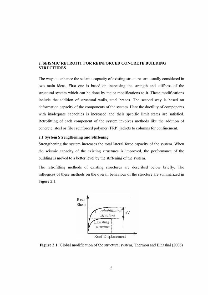
2.1 System Strengthening and Stiffening

Strengthening the system increases the total lateral force capacity of the system. When

the seismic capacity of the existing structures is improved, the performance of the

building is moved to a better level by the stiffening of the system.

The retrofitting methods of existing structures are described below briefly. The

influences of these methods on the overall behaviour of the structure are summarized in

Figure 2.1.

Figure 2.1: Global modification of the structural system, Thermou and Elnashai (2006)

6

The methods listed below are some of the repair and strengthening methods used for

existing concrete structures.

2.1.1 Shear walls

Placing of reinforced concrete shear walls into an existing building is one of the most

common methods used as repair and strengthening of structures. Although it increases

the strength and stiffness of vulnerable buildings it is necessary to evacuate the habitants

of the building during the construction.

Shear walls are efficient in controlling the overall lateral drifts and thereby reducing

damage in frame members. Application of shear walls involves partial or total infilling

of some of the bays of the frame. Existing infill walls can also be turned into shear walls

and shotcrete can be used instead of regular concrete to increase the adherence between

the existing and new material. To reduce time and cost, precast panels can be used as

well.

Many research on structural walls and results of detailed applications have been

reported, (Sugano and Fujimura 1980, Yuzugullu 1980, Higashi et al. 1980, Altin et al.

1992, Pincheira and Jirsa 1995, Frosh et al. 1996, Lombard et al. 2000, Inukai and

Kaminosono 2000). The results show that the response of panels with the structure

depends mainly on the application details. Proper anchorage of re-bars to beams and

closely spaced mesh increases the deformation abilities and the strength is increased by

full continuity between levels. If there is poor detailing and lack of load transfer between

old and new members, this may lead to brittle failure of infill panels or reduction of

ductility of the system.

One down side of the method is the need to strengthen the foundations. The

strengthening is necessary, so that the foundations can resist the increased weight of the

structure and the overturning moment. The application of this technique is usually

costly, disruptive and unsuitable for building with an insufficient foundation system.

2.1.2 Carbon fiber reinforced polymer (CFRP) applied on the infill wall

Another method used in the rehabilitation of reinforced concrete structures is

strengthening infill walls with fiber reinforced polymers (FRP). This technique improves

the seismic performance of structures in terms of strength, stiffness and energy

7

dissipation capacity. When it is compared with other techniques, it is very simple and

fast to apply and it is an efficient method because evacuation of the building is not

required during the process, however it is expensive.

Marshall and Sweeney (2004) tested the effect of FRP strengthening. They observed that

the failure mode of wall sections has also been changed by the different FRP

configurations. As can be seen by these tests, FRP composites can be applied to

increase the strength and change the failure mode of masonry walls in shear.

Erol et al. (2004, 2005, 2006 and 2008) performed a series of tests for examining the

differences between the structural behaviour of infilled RC frames strengthened by

CFRP fabric with different connection details. They observed that, the existence of

CFRP keeps the brittle wall to fall apart and hence contributes to the overall in-plane and

out- of-plane stability of structure during the load reversals.

2.1.3 Braced frames

Bracing frames with steel is one of the other methods to strengthen. However it does not

provide as much strength and stiffness as the shear walls method. Mass of braced frames

is less than the shear walls’ and they do not increase the building mass significantly.

Therefore seismic forces induced by the lateral load do not increase. Steel bracings are

usually installed between existing members and an improvement for the foundation

system might not be necessary.

It is difficult to connect bracing steel members to the existing concrete structure and the

connections are vulnerable during earthquakes. The addition of steel bracing is effective

for the strengthening and stiffening of existing buildings. In the selected bays of an RC

frame, to increase the lateral resistance of the structure, concentric or eccentric bracings

can be used.

Successful results of usage of steel bracing to upgrade RC structures have been reported

by several researches; (Sugano and Fujimura 1980, Higashi et al. 1984, Badoux and

Jirsa 1990, Miranda and Bertero 1990, Bush et al. 1991, Teran-Gilmore et al. 1995,

Pincheira and Jirsa 1995, Goel and Masri 1996). After the 1985 Michoacan Earthquake a

series of RC buildings retrofitted with steel bracing have been reported with no

structural damage (Del Valle 1980, Foutch et al. 1988).

8

Taşkın et al. (2007) have examined effects of different types of bracings with different

geometrical characteristics on the behavior of the system. In this study, instead of using

conventional bracing system, a new concept has been tested and compared with the

other systems. This approach is called as "Disposable Knee Bracing" and parametric

analytical studies done giving successful results. As expected bracing has increased the

horizontal load carrying capacity and energy absorption capacity, and most importantly,

reduced the amount of damage on the main structure. After obtaining these promising

results Yorgun et al. (2008) have done the experiments of these analytical models and

come up with close results.

To increase damping; shear links and passive energy dissipation devices may also be

used with bracings (Okada et al., 1992, Martinez-Romero, 1993). The addition of post-

tensioned rods, which will yield at smaller deformations to the system, will allow energy

dissipation at early stage of a large event. The initial brace prestressing induces

additional forces in the structure and the internal force distribution is modified. These

need to be considered for serviceability limit states.

2.1.4 Moment resisting frames

Moment resisting frames placed in buildings improve strength of the structure. Its

advantage is that they occupy minimum floor space. However they have large lateral

drift capacity when compared to the building they are placed in and this limits their use

and cause the main problem for the system.

2.1.5 Diaphragm strengthening

Diaphragm strengthening uses methods such as topping slabs, metal plates laminated

onto the top of the slab surface, bracing diaphragms below the concrete slabs and

increasing the existing nailing in the covering. The covering can be replaced with

stronger material or for buildings with timber diaphragms they could be replaced with

plywood.

2.2 Enhancing Deformation Capacity

To enhance deformation capacity; column jacketing, strengthening and providing

additional supports at places subjected to deformation are used. Below these will be

explained in detail.

9

The methods to increase the deformation capacity of existing structures are described

below briefly. How these methods affect the behaviour of the structure is summarized in

Figure 2.2.

Figure 2.2: Local modification of structural components, Thermou and Elnashai (2006).

2.2.1 Column strengthening

For building with strong beam-weak column configurations, column strengthening is

necessary as it will permit larger drifts and story mechanisms to be formed. In the

seismic performance of a structure, column retrofitting is often critical as columns

should not be the weakest components in the building structure. To increase the shear

and flexural strength of columns, column jacketing may be used so that columns will not

be damaged. The welding of the links between the new and existing reinforcement bars

only need specialist knowledge. Rodriguez and Park (1991), Al-Chaar et al. (1996),

Bousias et al. (2005), observed good results in their research.

Confining of columns with continuous steel plates and with fiber reinforced plastic

fibers are the two techniques that jacketing can be made. Recent research has also shown

the applications of composites especially fiber reinforced polymer (FRP) materials used

as jackets when retrofitting columns. As these jackets confine the columns, column

failure due to forming of a plastic hinge zone is prevented. The uncertainty of the bond

between the jacket and the original member is the main disadvantage of this method.

Jacketing up of the slab has to be done before the construction of the jacketing of the

column. If it is not done, then the load sharing does not take place until some large

10

seismic displacement has occurred. Until then this can cause considerable cracking, even

under small frequent earthquakes.

2.2.2 Local stress reductions

Local stress reductions are applied to the elements which do not effect the performance

of the building primarily. These can be done by demolition of local members that are not

stiff and introducing joints between face of the column and adjacent architectural

elements.

2.2.3 Supplemental support

Supplemental bearing supports are used on the gravity load bearing structural elements

which are not effective in resisting lateral force induced by an earthquake.

2.3 Reducing Earthquake Demands

Reducing earthquake demands involve new and expensive special protective systems

which modify the demand spectrum of the building while other methods improve the

capacity of the building. The special protective systems are appropriate to use for

important buildings such as historical buildings or for buildings which accommodate

valuable equipments and machinery.

Base isolation, energy dissipation systems and mass reduction are the methods used in

reducing earthquake demands will be explained briefly below.

2.3.1 Base isolation

In the upgrading of historical monuments, seismic isolation is accepted because it causes

minimal disturbances. It is also applied in the upgrading of RC structures which are

critical and need to be operational after seismic events. The aim of base isolation is to

isolate the structure from the ground motion during earthquakes. This is achieved by

installing bearings between the superstructure and its foundation. As most bearings have

good energy dissipation characteristics, this method is effective for relatively stiff

buildings with low rises and heavy loads.

Kawamura et al. (2000), applied seismic isolation technique to two middle-rise

reinforced concrete buildings in Japan. One is a 16 story building, which was upgraded

by lead rubber bearings (LRB's) were installed in their mid-height in 22 columns on the

8th story. Due to the reduction of seismic force by isolation, strengthening of the

11

structure is not necessary. The other building has 7 stories and is supported on piles,

where base isolation method was adopted. After cutting off the head of piles, rubber and

sliding isolators were installed in parallel. Therefore strengthening of the super structure

has come to be unnecessary.

Base or seismic isolation methods are efficient in reducing response acceleration and

interstorey drift which minimize structural and nonstructural damage.

2.3.2 Energy dissipation systems

Another method is using energy dissipation units (EDUs). These systems are used to

reduce the displacement demands on the structure by the energy dissipation and are most

effective when used in structures with great lateral deformation capacity. Frame

structures are appropriate for these systems. These systems can also be used to protect

critical systems and contents in a building.

Energy dissipation equipments are added to a structure via installing frictional,

hysteretic or visco-elastic dampers as parts of braced frames. Many researchers have

studied these energy dissipation methods, (Gates et al. 1990, Pekcan et al. 1995, Fu

1996, Tena-Colunga et al. 1997, Munshi 1998, Kunisue et al. 2000 and Kawamura et al.

2000). However, these methods are expensive and the application of them to all

structures is costly.

2.3.3 Mass reduction

Mass reduction which decreases the natural period of the building is one of the methods

used to lessen the demand on buildings. It can be done by removing some of the stories

in the building.

2.4 Rehabilitation Methods for Unreinforced Masonry Walls

Various rehabilitation methods for unreinforced masonry walls (URM) exist and they

can be listed as surface treatment, injection grouting, jacketing, internal reinforcement

and mechanical fasteners. They will be explained in detail below.

2.4.1 Surface treatment Surface treatment can be done by various materials and procedures. The most common

types of surface treatment involve using reinforced plaster, shotcrete and ferrocement

which are applied on top of a metal grid that is anchored to the existing wall. Hutchinson

12

et al. (1984) conducted experiments on various surface coatings to determine their

effectiveness in restoring and improving the in-plane strength of a damaged masonry

wall. They have concluded that they are usually effective.

Ferrocement is ideal for low cost housing since it is cheap and can be done with

unskilled workers. It consists of closely spaced multiple layers of mesh of fine rods

placed in a high strength (15-30 MPa) cement mortar layer of 10-50 mm thick. The

reinforcement ratio used is 3-8%. Usage of ferrocement improves both in-plane and out-

of-plane behavior of the wall. In-plane inelastic deformation capacity is improved as the

mesh helps confining the masonry units after cracking. Abrams and Lynch (2001) used

this retrofitting technique in a static cyclic test and observed that the in-plane lateral

resistance is increased by a factor of 1.5. Out-of-plane stability is improved as

ferrocement increases the ratio of the wall height-to-thickness.

Sheppard and Terceli (1980) used a thin layer of cement plaster which is applied over

high strength steel reinforcement for retrofitting. The steel reinforcement is usually

arranged as diagonal bars or vertical and horizontal meshes. This technique improves the

in-plane resistance in diagonal tension and static cyclic tests by a factor of 1.25 to 3. In

this method, the degree of masonry damage, strength of the cement mortar, thickness of

layer, the reinforcement quantity and how it is bonded with the retrofitted wall effect

how much improvement is achieved in strength.

Onto the masonry wall surface, shotcrete is sprayed over a mesh of reinforcement. When

shotcrete is compared with other cast in-situ jackets, it is more convenient and cost less.

Shotcrete thickness changes according to seismic conditions and it is at least 6 cm (Kahn

1984, Hutchison et al. 1984, Karantoni and Fardis 1992, Tomazevic 2000, Abrams and

Lynch 2001). Shear dowels which are 6 to 13 mm in diameter and 25 to 120 mm in

length are fixed into holes in the masonry wall using epoxy or cement grout. These are

used to transfer the shear stresses between shotcrete and masonry.

Some researchers think that epoxy is required to be used on the brick as to develop the

bond between shotcrete and the wall. Kahn (1984) has shown that dowels did not

improve the response of composite panels or the bond between brick and shotcrete. He

13

has also observed that wetting the surface of the wall before the application of shotcrete

did not affect the cracking or ultimate load. It slightly effects the inelastic deformations.

Using shotcrete on the retrofitted walls increases its ultimate load considerably. Kahn

(1984) used a 90 mm thick shotcrete on one side of the wall in a diagonal tension test

and found the ultimate load of URM panels to increase by a factor of 6.25. In a static

cyclic test conducted by Abrams and Lynch (2001), the ultimate load of the retrofitted

specimen increased by a factor of 3. They have observed contrary to Kahn (1984) that

the increase in the cracking load was irrelevant in a diagonal tension test after shotcrete

application.

Along with the advantages given above, there are some disadvantages in the application

of the shotcrete such as the need for special equipment, skill and the significant waste in

material due to rebound.

Application of shotcrete on the wall is assumed to resist lateral force applied to a

retrofitted wall and the brick masonry is ignored (Hutchison et al. 1984, Abrams and

Lynch 2001). This is reasonable as the flexural and shear strength of the reinforced

shotcrete can be more than that of the URM wall, but cracking in the masonry can occur

as the strains in the reinforcement in the shotcrete exceed yield. This can compromise

the performance objective for the immediate occupancy or operations to be continued

after a seismic event.

2.4.2 Injection grouting

Injection grouting is another method used as rehabilitation of unreinforced masonry

walls. It is usually applied to repair small cracks or to fill ungrouted cores. The main

purpose of injections is to restore the original integrity of the retrofitted wall and to fill

the voids and cracks, which are present in the masonry due to physical and chemical

deterioration and/or mechanical actions.

Epoxy is used for small cracks or small holes (less than 2 mm wide) and sand cement

mixed grout is used for larger holes (Calvi and Magenes 1994, Schuller et al. 1994). The

results of four clay brick walls which were repaired using injection grouting tested show

that the original strength of the wall prior to its damage was restored (Manzouri et al.

1996).

14

Holes and cracks are present in the masonry walls as it weakens due mechanical actions

or physical and chemical deterioration. Injection grouting is used to fill these and to re-

establish the integrity of the wall. Whether the grout mix can be injected which depends

on it mechanical and chemical properties or the method used affect the success of the

retrofit of the wall.

Schuller et al. (1994) found that a cement based grout injection can restore about 80% of

the compressive strength of the unretrofitted masonry. Other researchers reported that 80

to 110% of in-plane stiffness and 80 to 140% of in-plane lateral resistance of the

unretrofitted wall can be restored with that kind of injection (Sheppard and Terceli 1980,

Calvi and Magenes 1994, Manzouri et al. 1996). Also, the interface shear bond of multi-

wythe stonewalls can be amplified by a factor of 25-40 (Hamid et al. 1999). If epoxy is

used as an injection material, the retrofitted wall is usually stiffer than the unretrofitted

one, then the increase in stiffness which is 10-20% is much less than the increase in

strength. Lateral resistance of the retrofitted wall increases by a factor of 2-4.

2.4.3 Jacketing

Jacketing forms a frame around the damaged wall with cast in-place concrete or external

steel elements. For the existing URM buildings, steel plates or tubes can be used as

external reinforcement which can be attached directly to the existing diaphragm and

wall. Cracking in the masonry structure will occur in a seismic event and when this

reaches sufficient amount, the jacketed steel system will have comparable stiffness and

be effective (Hamid et al. 1994, Rai and Goel 1996).

Taghdi (2000a, 2000b) showed that the lateral in-plane resistance of the retrofitted wall

increases by a factor of 4.5 with the usage of vertical and diagonal bracing. This increase

is limited as the masonry is crushed and the vertical strips are buckled. The external steel

system presents an effective energy dissipation mechanism (Rai and Goel 1996, Taghdi

2000a, 2000b).

2.4.4 Reinforcing bars

Reinforcing bars are usually used in hollow walls where cores will be opened and a steel

bar will be placed inside and grouted. Prestressed tendons can also be used to improve

the performance of the wall (Lissel et al. 1998). The holes opened are vertical which

15

extent from the top of the wall to the basement wall. When it is grouted with the

reinforcing bar inside it, it provides a "homogeneous" structural element (Plecnik et al.

1986). This vertical column provides strength to the wall with a capacity to resist both

in-plane and out-of-plane loading and it is anchored to the roof and floors with lateral

ties.

The grout consists of a binder material like cement, polyester or epoxy and a filler

material like sand. Plecnik et al. (1986) have performed shear tests on cement grout

specimens which were 30% weaker than the ones with sand/epoxy or sand/polyester

grouts. When the cost is considered, it is better to use polyester keeping the volume ratio

of sand to polyester 1:1 and 2:1. Shear resistance depends on the volume ratios of the

components for cement-based grout. The best type of grout has a volume ratio of cement

to lime to sand of 1:0.125:1.

Abrams and Lynch (2001) used the reinforcing bars method to double the resistance of

URM wall in a static cyclic test. They have observed that even though the lateral

displacement achieved was high, the energy dissipated was limited. One advantage of

using this system as a retrofit method is that, it will not alter the appearance of wall

surface or the function of the building as it is done externally. The main disadvantage of

this method is that, it creates zones with widely varying stiffness and strength.

2.4.5 Mechanical anchors

Mechanical anchors or ties can be used between the wall and the surrounding structure

to provide better transfer of forces and continuity. Main disadvantage of this method is

that, steel bars corrode. Lissel and Shrive (2003) overcome this problem by introducing

fiber reinforced plastic.

Post-tensioning can be used to retrofit structures like historical monuments. This method

involves a compressive force applied to masonry wall which counteracts the tensile

stresses resulting from lateral loads. In the last ten years, there have been many

researches on post-tensioning globally (Karantoni and Fardis 1992, Ingham et al. 1998,

Lissel et al. 1999, Foti and Monac 2000, Laursen et al. 2002, Lissel and Shrive 2003,

Rosenboom and Kowalsky 2004, Schultz et al. 2003).

16

In and out of plane ultimate behaviors of wall, cracking load and distribution improve

when vertical post-tensioning is applied. Some basic calculations of principle stresses

show that the horizontal post tensioning improves the resistance. However the

experimental test performed by Page and Huizer (1994) did not prove these calculations.

Karantoni and Fardis (1992) show that horizontal post-tensioning of spandrels did not

significantly improve the building behavior by a linear finite element model they have

done. They also show that when horizontal and vertical post-tensioning is combined

together, the resulting positive effect is higher than the sum of the individual effects of

the two directions post-tensioning.

The methods discussed in this section need rigorous work and in some cases involve the

use of expert workmanship. They could be disruptive to the normal operation of a

building and some methods can add up to 15 cm thickness to the wall which could

require foundations to be improved. These may increase the inertial forces generated by

an earthquake.

2.5 What is Shotcrete

Spraying of concrete is applied first in the United States as early as 1907 and has been

known since. The product used was named “gunite” which was sprayed with easily

operated compressed air pumps. In some cases, instead of conventional concrete

shotcrete is used for its convenience, cost or time saving. It can be used when formwork

is expensive or not practical and access to the work area is difficult, thin layers or

variable thicknesses are required or normal casting techniques cannot be employed.

Shotcrete requires a small, portable plant for manufacture and placement and can be

applied in areas where limited access is available to make repairs in structures.

When shotcrete is accurately applied, it will show good bonding characteristics to

existing concrete, rock, steel and be a structurally sound and durable construction

material. If physical properties of shotcrete are compared with concrete or mortar with

the same composition, it is similar and sometimes better than them. It has low

absorption, good resistance to weathering and some chemical attacks, and high strength.

17

2.5.1 Types of shotcrete according to the application process

Types of shotcrete depend on which technique is used during its application. These are

dry and wet mix processes that will be explained in detail below.

a) Dry-mix process:

The dry-mix process is a method where the cement and aggregate are mixed either at a

site-based plant or pre-mixed and filled dried into silos or bags. This mixed material is

placed into a dry-mix sprayed concrete pump and by the help of compressed air, it is

brought to the nozzle. At the nozzle, the water necessary for hydration is added

depending on the judgment of the operator.

Dry-mix system is simple and it has been used in the past as there could be few

mechanical and mix design issues which can go wrong. The disadvantages of this

method are the dust generated from the system which has an impact on the environment,

the cost of wear of components of the machine used and the rebound of the material. The

rebound from the surface can be between 15% to 40%, and it can be reduced with the

usage of additives and admixtures. The capacity of machines effect the performance and

the properties of the sprayed concrete vary. The reason is the materials may not be

mixed properly, the cement-water ratios are unknown and changes and the mix might be

hydrated before it is brought to the pump.

b) Wet-mix process

As in the case of conventional concrete, a ready-mixed concrete is used. Therefore it is

possible to control the ratio of cement and water mixed, and the quality. The concrete

from the ready mix plant is placed into the pump, pushed through with pressure and at

the nozzle air is added at a rate between 7 to 15 m3/min, and the pressure used is 7 bars.

To achieve good compaction and adherence to the surface, the air is added to increase

the speed of the concrete.

The advantages of this method are 5 to 10% of aggregate rebound occurs, as low dust is

produced the working environment is better, and as admixtures are used, thick layers are

produced. Ratio of water to cement is controlled and can be as low as 0.37, and the

concrete can be considered as a permanent element of the structure. As the materials are

mixed before, change in quality is minimized and the effect of the operator is reduced.

18

Capacity of the output varies from 4 to 25 m3/hr, it is possible to add steel/synthetic

fibres and additives. The listed advantages make this method economical.

The disadvantages of the wet-mix are that the cleaning costs, limited conveying distance

which is maximum 300 m and the need for mix design. Also if it is not mixed on site,

the mixing plant has to be given the volumes of the mixtures and it has to be controlled

thoroughly.

2.5.2 Usage of shotcrete

Shotcrete can be used in other applications like repair of buildings, bridges, in

underground excavations, slope and surface protection, and in new structures.

Shotcrete is commonly used for repair of fire and earthquake damage and deterioration

and encasing structural steel for fireproofing. The repair of structural members such as

beams, columns, strengthening walls and connections is common for structures damaged

by an earthquake. It can also be used to repair the damaged surface of steel, wood or

concrete structures if the surfaces can be reached.

Shotcrete can be used to save time when thin sections and large areas are present in the

construction of new structures. These structures are pools, tanks, floors, walls and

domes. Zynda (2007) published a report about constructing a four-story parking garage

using shotcrete and precast beams, columns, and architectural walls. The project was

completed in record time with shotcrete application. Shotcrete was used throughout the

project, starting with the original shoring needed, the structural shear walls, and the 9.1

m-high retaining walls. Shotcrete is also used in forming and construction of structural

shotcrete walls and foundation walls, (Robbins 2004 and Von der Hofen 2008).

2.5.3 Types of shotcrete There are different types of shotcrete like fiber-reinforced, silica-fume, polymer-

modified and accelerated. These will be explained briefly below.

a) Fiber-reinforced shotcrete

When shotcrete is subjected to tensile stresses or strains, it will crack like the concrete if

it is not reinforced. Therefore fibers are added to the shotcrete mixtures to increase

capacity of energy absorption, impact resistance and ductility of the material. This

19

composite material will have an increased ultimate strength. Steel, glass or synthetic

fibers can be used in shotcrete.

• Steel fibers have been used since the late 1950s. Uniform distribution of fibers in

a mixture was caused by problems in mixing and handling them earlier. These

have been minimized by keeping the ratio of length to diameter low of the fibers

produced, surface deformations and improved shape.

• Glass-fibers and a resin binder are used together to obtain glass fiber reinforced

shotcrete. The application of this type of concrete requires a special gun and

equipment. This process is used extensively in the construction of lightweight

panels for building cladding and special architectural features and is usually

applied in a plant production situation.

• Nylon, polypropylene, polyethylene, polyester and rayon make synthetic fibers.

Decreasing the width of shrinkage cracks in the material is the primary benefit of

adding synthetic fibers to shotcrete.

b) Silica-fume shotcrete

Silica-fume which is a fine non-crystalline pozzolanic material that is mostly made up of

silica is used in shotcrete to increase strength. It also decreases permeability and enhance

cohesion and adhesion. Advantages of using silica-fume shotcrete are to improve the

bond strength between shotcrete and applied surfaces and cohesion. Thicker layers of

shotcrete can be applied in a single pass to surfaces whether vertical or overhead.

When silica-fume shotcrete is used, the rebound is significantly reduced and the action

of flowing water is reduced. Also this type of shotcrete can have more resistance to

aggressive chemicals.

Silica-fume shotcrete can be used in polymer modified and accelerated shotcrete

applications. It can be used in many applications instead of ordinary shotcrete due to its

high performance in bonding and strength.

Silica-fume shotcrete is used in construction of tunnels with fibers to control shrinkage

cracking.

20

c) Polymer-modified shotcrete

There are two methods to introduce polymers into shotcrete which are to use polymer

material as a binder and to form a continuous polymer matrix with replacing mixing

water with a polymer. In the first method, the shotcrete becomes a polymer shotcrete and

in the second one which is more common is to add a polymer emulsion to the hydraulic-

cement mixture and it is named as polymer-portland-cement shotcrete.

The polymers used in shotcrete improve tensile and flexural strengths, improve bonding

and reduce absorption.

d) Accelerated shotcrete

Accelerating admixtures are used in shotcrete to rapidly set shotcrete. These are

powdered materials added to dry-mix shotcrete which are called super-accelerators.

They can be powdered or liquid admixtures used in dry and wet-mix shotcrete. In the

wet-mix shotcrete usually the accelerator are added at the nozzle.

Accelerated shotcrete are used in tunnel support and linings, seawalls, dams, roof

construction, slope protection and water-retaining structures such as canals, thick

concrete sections, rapid repairs and sealing leaks.

21

3. TEST PROGRAM AND MATERIAL CHARACTERIZATION

This chapter describes the experimental test program that was carried out at STEEL

to evaluate the performance of a structural system consisting of shotcrete panel in

existing vulnerable RC frames. All test specimens are single story, single bay frames.

One bare frame and a conventional shear wall, three fully and three partially infilled

RC frames with shotcrete panels were tested. Description of the test specimens, test-

setup, data acquisition, instrumentation and material properties are presented here.

3.1 Test Specimens

In this study, panels made from wet-mixed shotcrete in lieu of a traditional masonry

are used to form an infill wall within existing vulnerable RC frame as shown in

Figure 3.1 and Figure 3.2. The RC frames were chosen to represent the weak

column/strong beam type structures that were very common in Turkey especially for

the buildings constructed before 1998 Turkish Earthquake Code. The specimens had

non-seismic details such as large spacing of hoops, no hoop in beam-column

connection region and no use of 135° seismic hooks.

Figure 3.1: General view of the fully infilled frame

22

Figure 3.2: General view of the partially infilled frame

Tested specimens are summarised in Table 3.1.

Foundations of the specimens are fixed to the adapter foundation through 28 φ50 mm

holes with φ39 mm anchorage bolts as shown in Figure 3.3. Depending on the

experiences obtained from other infilled frame experiments, the rocking and global

sliding of the frame does not occur during the experiments. Therefore the number of

φ39 mm anchorage bolts is enough to assume that the connection of foundation of

the specimens is similar to fixed supports.

One story, one bay nearly half-scale RC frames with a portion of slab on top and a

foundation at the bottom has been constructed in the laboratory. The cross sectional

dimensions of columns and beam of the frames are 20 cm by 25 cm and 20 cm by

32.5 cm, respectively. The height and the width of the frames are 152.5 cm and 220

cm, respectively. The height of the shotcrete panel is 170 cm and the width is 170 cm

and 130 cm. The dimensions and the reinforcement detail of the frames are given in

Figures 3.3 and 3.4. The details of panels are given in Figure 3.5. Longitudinal

reinforcement of the frames consist of 16 mm steel bars which have average yield

stress of 270 N/mm2, and the wire mesh used in the panels has a diameter of 4.5 mm

and yield stress of 320 N/mm2. The reinforcement ratio of the column and the panel

are %1.6 and %0.2 respectively.

Tab

le 3

.1: T

est s

peci

men

s

Spec

imen

Ty

pe

Fram

e co

nditi

on

Gap

spac

e be

twee

n pa

nel a

nd c

olum

ns

Pre-

reve

rse

defle

ctio

n

28 d

ay c

oncr

ete

com

pres

sive

st

reng

th (M

Pa)

Und

amag

ed

Dam

aged

&

repa

ired

Fr

ame

Pane

l

Spec

imen

1

YES

N

O

NO

N

O

16

-

Spec

imen

3

YES

N

O

NO

N

O

10

22

Spec

imen

5

YES

N

O

YES

N

O

12

35

Spec

imen

6

YES

N

O

NO

Y

ES

14

25

Spec

imen

7

Y

ES

NO

Y

ES

YES

12

25

δ δ

23

Table 3.1: Test specim

ens (contd.)

Specimen

Type Fram

e condition G

ap space between

panel and columns

Pre-reverse deflection

28 day concrete com

pressive strength (M

Pa)

Undam

aged D

amaged &

repaired

Frame

Panel

Specimen 2

YES

NO

N

O

NO

16

-

Specimen 2S

NO

Y

ES N

O

NO

16

35

Specimen 4

YES

NO

N

O

NO

12

Specimen 4S

NO

Y

ES Y

ES N

O

12 35

Specimen 8

YES

NO

N

O

NO

12

40

24

20

20

20 20

60

260

A

A

20

20

2525

Φ50

Col

umn

Cen

tre

30

260

38 17

0

220

32.5

12 20.5

120

b a

d c

20

20

20 20

60

260

AA

20

20

25

25Φ

50

Col

umn

Cen

tre

30

260

38

130220

32.5

12 20.5

120

b a

d c

2020

Fi

gure

3.3

: Geo

met

ry o

f the

spec

imen

s

25

26

B-B KESITI

120

205

325

mm

310 200 310820 mm

3? 16

10? 10

? 6/2003φ16

10φ10

φ6/200

Section b-b

250

200

25020

04? 16 5? 16

? 6 /200 ? 6 /200

C-C KESITI D-D KESITI

4φ16 5φ16

φ6/200 φ6/200

Section c-c Section d-d

120

205

325

mm

A-A KESITI

310 200 310820 mm

2? 16

1? 1610? 10

? 6/2002φ16

1φ1610φ10

φ6/200

Section a-a

130

5 φ4.5

Section e-e

Figure 3.4: Reinforcement details of the frame

Figure 3.5: Reinforcement details of the panel

Section A

5cm

A

170cm

Wire mesh Q 106/106

27

Longitudinal reinforcement of the columns continues to the bottom of the

foundations of the specimens which are 38 cm thick. There is no lap-splice at the

level of foundation.

Specimen 1 is the bare frame which is tested as a reference specimen.

Specimens 2 and 4 are the bare frames which are tested up to a certain damage level,

before constructing the shotcrete panel in Specimens 2S and 4S. These bare frames

are tested till 10.5 cm-displacement which is the displacement level at which the

main reinforcement yield. These damaged bare frames are repaired by injection of

epoxy into the cracks which were formed at different locations of the columns

following the subsequent steps below;

- 10 cm deep holes are drilled at the edge of the cracks,

- the steel dowels are fixed into these holes by using epoxy resin as can be seen

in Figures 3.6b and 3.6c,

- at least 8 hours later, the epoxy resin are injected into these dowels and all

these cracks are filled with epoxy resin as can be seen in Figures 3.6d and

3.6e.

After that, a wire mesh (Q 106/106) consisting of Ф4.5 mm steel bars is placed at the

center axis of the frame. Full contact of the panel is established by lapping the infill

reinforcement to the anchorages placed in the frame members. The anchorages used

are Ф10 mm steel bars which are placed in the beam of the frame 20 cm apart from

each other in partially infilled frames by epoxy resin. In fully infilled frames, the

anchorages are placed in the beam and the columns 30 cm apart from each other. The

lengths of the anchorages are 35 cm; 25 cm of it is in the panel while 15 cm is in the

beam. By using wet-mixed sprayed concrete, 5 cm thick RC panel is formed as

shown in Figure 3.7. The panel formed is attached to the frame by all sides to form

Specimen 2S while in Specimen 4S, the panel is attached only to the beams and the

panel is placed 20 cm to the columns.

Construction of Specimens 3, 5, 6 and 7 are identical except that the RC frames were

not damaged.

Specimen 5 is identical to Specimen 4S in which the shotcrete panel is only

connected to the beams, not connected to the columns and is placed 20 cm away

28

from the columns as shown in Figure 3.7. Shotcrete panel is constructed in a non-

damaged frame. While deciding the width of this panel, the region on the beam

where moment is supposed to be small under lateral and vertical loads is taken into

account.

Figure 3.6: Repairing process of the damaged bare frames

Although the construction of Specimens 6 and 7 are similar to the others explained

above, pre-reverse deflection is applied to the beam during construction of the

shotcrete panel as can be seen in Figure 3.8. Before constructing the shotcrete panel,

special screws are placed symmetrically to the right and left side of the beam in the

middle between the foundation and the floor. Pre-reverse deflection applied to both

specimens is 7.4 mm and it was applied with mechanical force which is produced by

the screws. The idea behind the amount of the pre-reverse deflection is that after the

application of the pre-reverse deflection, the cracks that will occur in beams and

columns to be small in width and therefore no special repairing will be needed.

Considering this fact, some calculations are done and the reasonable amount of the

pre-reverse deflection is found to be 1/300-1/250 of the span. In Specimen 6, the

(a)

(b) (c)

(d) (e)

29

panel is connected to the surrounding frame by all its four sides, while in Specimen 7

the panel is connected only to the beams.

During the process, the deflection is continuously measured in the middle of the

beam with a displacement transducer. As expected, shear cracks at columns and

flexural cracks at the tension side of the beam occurred during pre-reverse deflection

process. The amount of deflection is 7.4 mm which is almost 1/260 of the span. The

maximum crack width occurred is 0.1 mm on the columns and 0.4 mm on the beam.

By applying the pre-reverse deflection to the beam; the shotcrete panel and the frame

around it, are supposed to work together for a long time ensuring that the lateral

loads are transferred better through the system.

Figure 3.7: Construction of the shotcrete panels

30

Specimen 8 is a typical shear wall having the same reinforcement as the shotcrete

panels which can be seen in Figure 3.9. Two layers of formwork are used and the

concrete is poured from right beside the beam. The concrete of the shear wall is

prepared in Construction Materials Laboratory of ITU Civil Engineering Faculty.

After removing the formwork of the shear wall, some gaps were present at the upper

side of the wall where the concrete is poured from. Therefore these gaps are fixed

with “repairing mortar”.

Figure 3.8: Specimens 6 and 7 having pre-reverse deflection on beam

Figure 3.9: Construction of Specimen 8

Special screws

31

3.2 Test Setup, Instrumentation and Data Acquisition

Test setup, instrumentation and data acquisition system are described in this section.

Details of the test setup including figures and experimental requirements are given in

the following subsections.

3.2.1 Test setup and loading system

A typical test-setup is shown in Figure 3.10. Axial load which is kept constant

throughout the test is applied on the columns and lateral cycling load imposed as

displacement reversals is applied to the specimen by means of a hydraulic jack and

two MTS 250 kN-capacity hydraulic actuators that are placed at the beam level,

respectively.

Figure 3.10: Test setup

The physical capacities of one actuator for load are ±250 kN and for displacement is

±300 mm. Controlling of actuators are force-based or displacement-based. The data

collected during the tests are force and displacement of the actuators, and the

displacements taken by the linear variable displacement transducers (LVDT)

connected to various positions on the specimen. Displacement-based load protocol

32

was used during the tests. The high sensitive LVDT which has measured top

displacement of the specimen was assigned as the control displacement.

The axial loading system works independently from the lateral loading system. The

axial loads acting on two columns of the specimen are the support reactions of the

rigid steel beam placed on top of the specimen. The required axial load level is

controlled by a hydraulic jack and a load cell placed on steel beam. The intensity of

the axial load which is kept constant throughout the test is 20 % of the axial load

carrying capacity of columns.

3.2.2 Instrumentation and data acquisition

LVDTs are placed on some critical positions to measure the displacements and

deformations of the specimens. The applied load and displacement of the hydraulic

actuator are also measured and recorded. The LVDTs are connected to a TML ASW

50C switch-box and TDS 302 data logger, which provide AC power, signal

amplification, AC-to-DC conversion and electrical balancing.

The number of LVDTs used, their types and the measurement purpose are listed in

Table 3.2 and their places are shown in Figure 3.11 for bare frame; in Table 3.3 and

in Figure 3.12 for fully infilled frames and in Table 3.4 and in Figure 3.13 for

partially infilled frames. The rotation of the columns and the wall, the relative

displacement of the whole specimen and the frame, the target displacement which is

watched through two channels that is the relative top displacement of the specimen,

the top displacements of the column and the wall, the out of plane behaviour of the

specimen, elongation and shortening of the wall are measured. For the specimens

with pre-reversed beam, six more LVDTs are placed on the specimens. The two of

them are for measuring the displacement of reversely deflected beam and four of

them are for measuring the axial deformation of the columns.

33

Table 3.2: LVDTs used for bare frame

Name LVDT type Measurement purpose Attached to T1 CDP5 Top displacement Reference frame T2 CDP25 Top displacement Reference frame T3 CDP5 Displacement of the whole system Reference frame T4 CDP5 Displacement of the frame Reference frame T5 CDP25 Column displacement Reference frame T6 CDP25 Out of plane displacement Reference frame T7 CDP10 Column lower rotation Specimen T8 CDP10 Column lower rotation Specimen T9 CDP10 Column lower rotation Specimen T10 CDP10 Column lower rotation Specimen T11 CDP10 Column upper rotation Specimen T12 CDP10 Column upper rotation Specimen T13 CDP5 Column upper rotation Specimen T14 CDP5 Column upper rotation Specimen

Table 3.3: LVDTs used for fully infilled frame

Name LVDT type Measurement purpose Attached to

T1 CDP25 Top displacement Reference frame T2 CDP100 Top displacement Reference frame T3 CDP5 Panel displacement Reference frame T4 CDP25 Column displacement Reference frame T5 CDP100 Panel front diagonal Specimen T6 CDP5 Panel back diagonal Specimen T7 CDP50 Displacement of the frame Reference frame T8 CDP25 Displacement of the whole system Reference frame T9 CDP25 Right column lower rotation Specimen T10 CDP25 Right column lower rotation Specimen T11 CDP25 Panel rotation Specimen T12 CDP25 Panel rotation Specimen T13 CDP25 Panel rotation Specimen T14 CDP25 Left column lower rotation Specimen T15 CDP25 Left column lower rotation Specimen T16 CDP10 Out of plane displacement Reference frame T17 CDP10 Right column upper rotation Specimen T18 CDP10 Right column upper rotation Specimen T19 CDP10 Left column upper rotation Specimen T20 CDP10 Left column upper rotation Specimen

34

Front view

T11 T12 T13 T14T5

T1T2

T7 T8 T9 T10T3

Back view

T4

T6

Figure 3.11: Locations of LVDTs on bare frames

Front View

T20 T19 T18 T17

T16 T4 T3

T2T1

T15 T14 T13 T12 T11 T10 T9 T8

T5

Back View

T7

T6

Figure 3.12: Locations of LVDTs on fully infilled frames

Front view

T9

T2 T1

T3

T6

T8 T10 T11

T12 T13 T14 T15

T16 T17T18 T19

T20

T21

T22

T5

T7

Back view

T4 T5

T23

Figure 3.13: Locations of LVDTs on partially infilled frames

35

Table 3.4: LVDTs used for partially infilled frame

Name LVDT type Measurement purpose Attached to

T1 CDP25 Top displacement Reference frame T2 CDP100 Top displacement Reference frame T3 CDP5 Displacement of the whole system Reference frame T4 CDP5 Displacement of the frame Reference frame T5 CDP5 Displacement of the frame Reference frame T6 CDP100 Column displacement Reference frame T7 CDP50 Out of plane Reference frame T8 CDP25 Right column lower rotation Specimen T9 CDP25 Right column lower rotation Specimen

T10 CDP25 Left column lower rotation Specimen T11 CDP25 Left column lower rotation Specimen T12 CDP25 Right column upper rotation Specimen T13 CDP25 Right column upper rotation Specimen T14 CDP25 Left column upper rotation Specimen T15 CDP25 Left column upper rotation Specimen T16 CDP10 Panel rotation Reference frame T17 CDP10 Panel rotation Reference frame T18 CDP10 Panel rotation Reference frame T19 CDP10 Displacement of the bottom part of panel Reference frame T20 CDP25 Displacement of the middle part of panel Reference frame T21 CDP25 Displacement of the top part of panel Reference frame T22 CDP10 Panel front diagonal Specimen T23 CDP10 Panel back diagonal Specimen

3.3 Load Pattern

Since the loading is to simulate the effect of seismic action, reversed cycling loading

is applied to all specimens. Displacement reversals with increasing intensity are

applied to the specimens by actuators. Up to 0.467 mm top displacement, the target

values are applied once on the specimens observing the elastic behaviour of the

specimens. After this step, each displacement cycle is repeated thrice for both

forward and backward cycles. At the end of each displacement target, the occurred

cracks are marked.

The details of the loading protocol are presented in Table 3.5 and Figure 3.14.

36

Table 3.5: Steps of the loading protocol

Load level Top displacement Relative Story Drift [mm] δ/H 1 0.035 0.000025 2 0.070 0.000050 3 0.140 0.000100 4 0.280 0.000200 5 0.350 0.000250 6 0.467 0.000300 7 0.700 0.000500 8 1.400 0.001000 9 2.800 0.002000 10 3.500 0.002500 11 4.200 0.003000 12 4.900 0.003500 13 5.600 0.004000 14 7.000 0.005000 15 10.500 0.007500 16 14.000 0.010000 17 28.000 0.020000 18 42.000 0.030000

-45

-30

-15

0

15

30

45

Step

Top

Disp

lace

men

t (m

m)

δ/H=3%

δ/H=2%

δ/H=1%

Figure 3.14: Loading protocol

3.4 Material Tests

Samples of materials used in the specimens were tested to determine their

mechanical properties because success of the numerical models is highly dependent

on correctly defining the material characteristics.

37

3.4.1 Concrete tests

Mix proportions of concrete used for constructing the frames and the shotcrete panels

are given in Table 3.6 and Table 3.7, respectively. Compressive strengths of the

concrete were obtained from compressive tests on standard cylinders (150 mm*300

mm) taken at various stages of the construction. Minimum of three standard

cylinders were tested for each specimen. The compressive strength of the concrete

used in the numerical models was the average values obtained from these tests.

Results are summarised in Table 3.8 for the frame concrete and in Table 3.9 for the

shotcrete panel concrete.

All cylinders were tested at the Construction Materials Laboratory of ITU Civil

Engineering Faculty using a 5000 kN capacity Amsler compression press. Concrete

cylinders were loaded in compression at a rate of 0.02 mm/min.

Table 3.6: Concrete mix proportions for frame concrete

Material Weight for one cubic meter Portland Cement 300 kg (32.5 R)

Water 140 kg Sand 690 kg

Gravel 1070 kg (No:1)

Table 3.7: Concrete mix proportions for shotcrete panel concrete

Material Weight for one cubic meter Portland Cement 400 kg (42.5 R)

Water 300 kg Sand 900 kg

Gravel 600 kg (No:2)

Table 3.8: The average concrete compressive strengths for frames

Name of specimen

Number of samples

Compressive strength [MPa]

1 3 16 2 3 16 3 4 10 4 3 12 5 3 12 6 3 14 7 3 12 8 3 12

38

Table 3.9: The average concrete compressive strengths for panels

3.4.2 Steel reinforcement tests

Tensile tests were carried out to determine the mechanical characteristics of each

type of reinforcing bar used in the specimens. All the samples were tested at the

Material Testing Laboratory of ITU Civil Engineering Faculty using Amsler testing

machine of 200 kN tension capacity. Free length between the two heads of the

machine was chosen as 10φ. Locations of the bars tested in test specimens are given

below:

1) φ16 bars are used as longitudinal reinforcement for the columns and the

beams,

2) φ10 bars are used as longitudinal reinforcement for the slabs and dowel bars,

3) φ6 bars are used as stirrups for frames.

Three samples were taken from each type of reinforcement. Mechanical properties of

these bars obtained from the tests are summarised in Table 3.10. Values given in the

table are the average of the three samples tested.

Table 3.10: Mechanical properties of steel bars

Name of specimen

No. of samples

Compressive strength [MPa]

2S 3 35 3 3 22

4S 3 35 5 3 35 6 3 25 7 3 25 8 3 40

Diameter [mm] φ16 φ10 φ6 σy [MPa] 270 290 325

σmax [MPa] 420 450 481 εsu [mm/mm] 0.25 0.30 0.35

39

4. EXPERIMENTAL RESULTS

Although there are several measurement points on the specimens, the top

displacements versus base shear relationships and some of the graphs drawn for the

critical sections and damage modes are selected to be presented here. Through

Section 4.1 to 4.9, the results are also compared with Specimen 1 (bare frame)

results. Since some of the specimens don’t have the same concrete compressive

strength unintentionally as presented in Table 3.1; the analytical bare frame, which is

explained in detail in Chapter 5, having identical concrete compressive strength as

the retrofitted specimens are also introduced into the comparison of envelope curve

diagrams. This will help to have a more accurate comparison and evaluation of the

test results. In Section 4.10; all specimens are compared with each other according to

their failure modes, lateral load carrying capacity, initial stiffness, dissipated energy,

ductility and stiffness.

4.1 Test Results of Specimen 1

This specimen is the bare frame used as a reference frame and the effect of the

different strengthening methods is compared and discussed with this specimen’s

results. The types of the LVDTs and what was measured by them on the bare frame

was given in Table 3.2 and Figure 3.11.

The largest displacement applied to the specimen was 42 mm in both pulling and

pushing displacement cycles. The axial load applied on each column was 165 kN

which equals to 20% of the axial load carrying capacity of the column.

Base shear versus top displacement diagram is given in Figure 4.1. The maximum

strengths in tension and compression are 133 kN and 123 kN, respectively, obtained

at 28 mm cycles which correspond to 2% story drift. The envelope curve of the base

shear-top displacement relationship is also given in Figure 4.2. The data of envelope

curve are calculated as the average of the three cycles at each target displacement

levels given in Table 3.5. As it is seen in Figure 4.2, the maximum story drift reached

40

is 3% where the lateral load carrying capacities of the frame are 104 kN and 86 kN in

tension and compression, respectively.

-50 -40 -30 -20 -10 0 10 20 30 40 50-200

-100

0

100

200B

ase

Shea

r [k

N]

Displacement [mm] Figure 4.1: Base shear-top displacement curve of Specimen 1

-56 -42 -28 -14 0 14 28 42 56-200

-100

0

100

200-0.04 -0.03 -0.02 -0.01 0.00 0.01 0.02 0.03 0.04

Bas

e Sh

ear

[kN

]

Displacement [mm]

Drift

Figure 4.2: Envelope curve of Specimen 1

Rotation at the critical sections is calculated as the sum of displacement values (∆1,

∆2), measured from the two LVDTs placed at 12.5 cm from the end of the column,

divided by the column width, x, as seen in Figure 4.3.

The rotation is calculated using Equation 4.1;

θ = (∆1+∆2) / x (4.1)

41

Figure 4.3 Calculation of rotation at the ends of the columns

In Figures 4.4, base shear versus bottom end rotation of right (the one that is near to

the actuator) and left columns and in Figures 4.5 base shear versus top end rotation

of the right and left columns are given, respectively.

The maximum rotations obtained at the column sections are about 0.02 radian. At the

top end of the right column when the rotation is 0.01 radian, the corresponding load

at that level is 133 kN. At the bottom end of the right column when the rotation is

0.01 radian, the corresponding load at that level is 106 kN.

-0.04 -0.02 0.00 0.02 0.04-200

-100

0

100

200

Bas

e Sh

ear

[kN

]

Rotation

-0.04 -0.02 0.00 0.02 0.04-200

-100

0

100

200

Bas

e Sh

ear

[kN

]

Rotation

Figure 4.4: Rotation at the bottom end of the right and left column

-0.04 -0.02 0.00 0.02 0.04-200

-100

0

100

200

Bas

e Sh

ear

[kN

]

Rotation-0.04 -0.02 0.00 0.02 0.04

-200

-100

0

100

200

Bas

e Sh

ear

[kN

]

Rotation Figure 4.5: Rotation at the top end of the right and left column

Before deformationAfter deformation

42

Crack pattern of the specimen after test is given in Figure 4.6 and Table 4.1 shows

the width of cracks at specific drift ratios.

Figure 4.6: Crack pattern of Specimen 1 at the end of test

Table 4.1: Width of cracks in mm at specific story drifts

Crack no Drift = 1% Drift = 2% Drift = 3% 1 1.6 3.0 - 2 0.6 1.4 >3.5 3 0.1 0.1 0.2 4 1.2 2.5 - 5 0.5 0.9 0.9 6 0.2 0.9 - 7 0.15 1.4 3.4 8 0.3 1.0 >3.5 9 0.1 1.4 3.5 10 - 0.2 0.9


This is a bare frame which is tested up to a certain damage level before strengthening

with shotcrete panel to form Specimen2S. The types of the LVDTs and what was

measured by them on the bare frame was given in Table 3.2 and Figure 3.11.

The specimen was tested up to 10.5 mm which is the displacement level at which the

longitudinal reinforcement of the columns started to yield in previous experiments.

The axial load applied on each column was 162.5 kN which equals to 20% of the

axial load carrying capacity the column.

Push Pull

1 23 4

5

6 78

9

10

43

Base shear versus top displacement diagram is given in Figure 4.7. The envelope

curve of the hysteretic response of the specimen is given in Figure 4.8.

-50 -40 -30 -20 -10 0 10 20 30 40 50-200

-100

0

100

200

Bas

e Sh

ear

[kN

]

Displacement [mm]

Figure 4.7: Base shear-top displacement curve of Specimen 2

-56 -42 -28 -14 0 14 28 42 56-200

-100

0

100

200-0.04 -0.03 -0.02 -0.01 0.00 0.01 0.02 0.03 0.04

Bas

e Sh

ear

[kN

]

Displacement [mm]

Drift

Figure 4.8: Envelope curve of Specimen 2

In Figures 4.9, bottom end rotation of right and left columns and in Figures 4.10, top

end rotation of right and left columns versus base shear are given, respectively.

Inelastic behaviour has started at bottom ends of the columns, while top ends stayed

elastic.

44

-0.04 -0.02 0.00 0.02 0.04-200

-100

0

100

200

Bas

e Sh

ear

[kN

]

Rotation-0.04 -0.02 0.00 0.02 0.04

-200

-100

0

100

200

Bas

e Sh

ear

[kN

]

Rotation


-0.04 -0.02 0.00 0.02 0.04-200

-100

0

100

200

Bas

e Sh

ear

[kN

]

Rotation-0.04 -0.02 0.00 0.02 0.04

-200

-100

0

100

200

Bas

e Sh

ear

[kN

]

Rotation

Figure 4.10: Rotation at the top end of the right and left column

Crack pattern of the specimen after test is given in Figure 4.11. Table 4.2 shows the

width of cracks at specific drift ratios.


Push Pull

6

55 3

8

1

2

7 4

45

Table 4.2: Width of cracks in mm at specific story drift

Crack No: Drift = 0.5% 1 0.6 2 0.2 3 0.8 4 0.8 5 0.9 6 0.6 7 0.9 8 0.5

4.3 Test Results of Specimen 2S

The observed cracks of Specimen 2 was repaired with epoxy resin and retrofitted

with a shotcrete panel and named as Specimen 2S. The types of the LVDTs and what

was measured by them for the specimen are given in Table 3.3 and Figure 3.12.

The largest displacement applied was 28 mm. The axial load applied on each column

was 162.5 kN which equals to 20% of the axial load carrying capacity of the column.


strengths in tension and compression are 342 kN and 394 kN, respectively, occurred

at 2% story drift which is also the maximum story drift reached. The ultimate lateral

load carrying capacities corresponding to the maximum drifts of the frame are 166

kN and 249 kN in tension and compression, respectively. The envelope curve of the

hysteretic response of the specimen is given in Figure 4.13.

-30 -20 -10 0 10 20 30-400

-300

-200

-100

0

100

200

300

400

Bas

e Sh

ear

[kN

]

Displacement [mm]

Figure 4.12: Base shear-top displacement curve of Specimen 2S

46

-42 -28 -14 0 14 28 42-400

-300

-200

-100

0

100

200

300

400-0.03 -0.02 -0.01 0.00 0.01 0.02 0.03

Drift

Bas

e Sh

ear

[kN

]

Displacement [mm]

Figure 4.13: Envelope curve of Specimen 2S

In Figures 4.14, bottom end rotation of right and left column and in Figures 4.15, top

end rotation of right and left columns versus base shear are given, respectively. At

the top end of the right column when the rotation is 0.01 radian, the corresponding

load at that level is 250 kN. At the bottom end of the right column when the rotation

is 0.01 radian, the corresponding load at that level is 290 kN.

-0.04 -0.02 0.00 0.02 0.04-400-300-200-100

0100200300400

Bas

e Sh

ear

[kN

]

Rotation

-0.04 -0.02 0.00 0.02 0.04-400-300-200-100

0100200300400

Bas

e Sh

ear

[kN

]

Rotation Figure 4.14: Rotation at the bottom end of the right and left column

-0.04 -0.02 0.00 0.02 0.04-400-300-200-100

0100200300400

Bas

e Sh

ear

[kN

]

Rotation

-0.04 -0.02 0.00 0.02 0.04-400-300-200-100

0100200300400

Bas

e Sh

ear

[kN

]


47

The observed maximum displacement in the shotcrete panel is 5 mm in pushing and

10 mm in pulling sides as seen in Figure 4.16. Figure 4.17 shows the specimen at the

end of the test and the crack patterns of all specimens at the ultimate state are given

in Figure 4.18.

-30 -20 -10 0 10 20 30-400

-300

-200

-100

0

100

200

300

400B

ase

Shea

r [k

N]

Displacement [mm]

Figure 4.16: Panel displacement

Nominal shear stress of the shotcrete panel is calculated using Equation 4.2,

τ = eft

s

AQ

(4.2)

where Qs is the specific load obtained. Aeft is the total area, which is the sum of cross

sections of the panel and columns, which resist the shear forces.

Maximum load that has occurred at the end of the pushing displacement cycles was

342.5 kN and in the pulling displacement cycles was 393.5 kN. The nominal shear

stresses corresponding to these values are 1850 kN/mm2 and 2127 kN/mm2. The first

cracks observed in the system were the shear crack at the bottom end of the column

which was closer to the actuators that have been repaired by epoxy injection, the

shear crack at the top of the same column and the separation of this column from

beam. These cracks were observed during the displacement cycle of +0.467 mm. The

load was reported as 107 kN where the nominal shear stress is 578 kN/mm2. The first

separation between the panel and the frame members occurred during the

displacement cycle of +0.7 mm. The load was reported as 132 kN where the nominal

shear stress is 713 kN/mm2 at that state. The first diagonal crack was observed on

48

the panel during the -0.467 mm cycles. In that cycle, the load was 55 kN. Maximum

displacement of the panel recorded was 5 mm in the positive displacement cycles and

10 mm in the negative ones. The widths of the cracks observed are given in Table

4.3.

Figure 4.17: Specimen 2S at the end of test

Figure 4.18: Crack pattern of Specimen 2S at the end of test

1

2

38

6

5

4

79

Push Pull

49


Crack No: Drift = 1% Drift = 2% 1 1.4 2 0.3 >3.5 3 >3.5 >3.5 4 1.6 5 >3.5 >3.5 6 1.6 7 >3.5 >3.5 8 >3.5 >3.5 9 >3.5 >3.5

Comparison of the results of the retrofitted frame with shotcrete panel with the bare

frames’ are given below. In Figure 4.19 and Tables 4.4 and 4.5, the comparison of

the load carrying capacity; in Table 4.6 the comparison of initial stiffnesses, in

Figure 4.20 and 4.21 the comparison of energy dissipation capacities of both frames

are summarised.

-56 -42 -28 -14 0 14 28 42 56-400

-300

-200

-100

0

100

200

300

400-0.04 -0.03 -0.02 -0.01 0.00 0.01 0.02 0.03 0.04

Bas

e Sh

ear

[kN

]

Displacement [mm]

Specimen 1 Specimen 2S

Drift

Figure 4.19: Comparison of envelope curves of Specimen 2S and Specimen 1

Table 4.4: Effect of strengthening in general Specimen

name Failure mode +P max

(kN) +∆ max

(mm) -P max

(kN) −∆ max

(mm) +Pult

(kN) -Pult

(kN) ∆ulti

(mm)

Specimen 1 Bending + Shear failure at column ends 133 28 -123 -28 104 -86 42

Specimen 2S Shear failure at column ends 342 28 -394 -28 166 -249 28

50

In Table 4.4, +Pmax and –Pmax indicates the maximum loads occurred during pushing

and pulling cycles, while +∆max is the displacement corresponds to +Pmax and -∆max

the displacement corresponds to -Pmax during the experiment. +Pult and –Pult are

residual lateral load carrying capacity of the system at the end of the test. ∆ult is the

displacement level at which the experiment ends.

Table 4.5: Maximum base shears recorded during the tests

Maksimum load [kN]

Proportion ratio Specimen name

Push Pull Push Pull Specimen 1 133 -123 1.0 1.0

Specimen 2S 342 -394 2.6 3.2

Table 4.6: Initial stiffness of the specimens

0 10 20 30 40 500

20000

40000

60000

80000

Cum

ulat

ive

Ene

rgy

Dis

sipa

tion

[kN

mm

]

Displacement [mm]


Figure 4.20: The comparison of cumulative energy dissipation capacities of

Specimens 1 and 2S

Specimen name Initial stiffness [kN/mm]

Proportion ratio

Specimen 1 22.0 1.0 Specimen 2S 231.0 10.7

51

0

10000

20000

30000

40000

50000

60000

70000

0.01 0.02 0.03

Drift

Cum

ulat

ive

Ene

rgy

Diss

ip[k

Nm

m]

Specimen 2SSpecimen 1

Cum

ulat

ive

Ene

rgy

Dis

sipa

tion

[kN

mm

]

Figure 4.21: Cumulative energy dissipation capacities of Specimens 1 and 2S at

various story drifts

The results are summarised below:

• The lateral stiffness of the frames, right before the first cracks occurred in the

system, increased by 10.7 times for Specimen 2S compared with the bare frame’s

as seen in Table 4.6.

• The lateral load carrying capacity increased by between 2.6 to 3.2 times for the

specimens with shotcrete panel compared with the bare frame’s as seen in Figure

4.19 and Table 4.4 and 4.5.

• Comparison of Figures 4.14 and 4.15 with Figures 4.4 and 4.5,

• At the top end of the right column when the rotation is 0.01 radian, the

corresponding load at that level for Specimen 1 is 133 kN while for

Specimen 2S is 250 kN which is almost 1.9 times of the bare frame’s,

• At the bottom end of the right column when the rotation is 0.01 radian,

the corresponding load at that level for Specimen 1 is 106 kN while for


• The cumulative energy dissipation of the Specimen 2S at 1% story drift are 10

times, at 2% story drift are 5.5 times compared to the bare frame’s shown in

Figure 4.20 and 4.21.

52


This is the RC frame retrofitted with shotcrete panel which is connected to frame at

all four sides. The types of the LVDTs and what was measured by them for

Specimen 3 are given in Table 3.3 and Figure 3.12.


was 112.5 kN which equals to 20% of the axial load carrying capacity the column.



at 10.5 mm cycles which correspond to 0.75% story drift. The maximum story drift

reached is 1%. The lateral load carrying capacities corresponding to maximum story

drift reached are 165 kN and 136 kN in tension and compression, respectively.

The envelope curve of the hysteretic response of the specimen is given in Figure

4.23.

-30 -20 -10 0 10 20 30-400

-300

-200

-100

0

100

200

300

400

Bas

e Sh

ear

[kN

]

Displacement [mm]

Figure 4.22: Base shear-top displacement curves of Specimen 3

53

-42 -28 -14 0 14 28 42-400

-300

-200

-100

0

100

200

300

400-0.03 -0.02 -0.01 0.00 0.01 0.02 0.03

Drift

Bas

e Sh

ear

[kN

]

Displacement [mm] Figure 4.23: Envelope curve of Specimen 3

In Figures 4.24, bottom end rotation of right and left columns and in Figures 4.25,

top end rotation of the right and left columns versus base shear are given,

respectively.

-0.04 -0.02 0.00 0.02 0.04-400-300-200-100

0100200300400

Bas

e Sh

ear

[kN

]

Rotation

-0.04 -0.02 0.00 0.02 0.04-400-300-200-100

0100200300400

Bas

e Sh

ear

[kN

]

Rotation


-0.04 -0.02 0.00 0.02 0.04-400-300-200-100

0100200300400

Bas

e Sh

ear

[kN

]

Rotation-0.04 -0.02 0.00 0.02 0.04

-400-300-200-100

0100200300400

Bas

e Sh

ear

[kN

]


54

-30 -20 -10 0 10 20 30-400

-300

-200

-100

0

100

200

300

400

Bas

e Sh

ear

[kN

]

Displacement [mm] Figure 4.26: Panel displacement

Maximum load that has occurred at the end of the positive displacement cycles was

290 kN and in negative displacement cycles was 279 kN. The nominal shear stresses

corresponding to these values are 1568 kN/mm2 and 1508 kN/mm2. The first

separation between the panel and the frame members and also the first diagonal crack

observed during the +1.4 mm cycles. The load was reported as 85 kN where the

nominal shear stress corresponds to 460 kN/mm2 at that state. In the later cycles,

several cracks occurred parallel to this crack. The first shear crack occurred at the

upper end of the right column during +2.8 mm cycles. The load was reported as 147

kN where the nominal shear stress corresponds to 795 kN/mm2 at that state.

Maximum displacement of the panel recorded was 6 mm in the positive displacement

cycles and 5.5 mm in the negative ones shown in Figure 4.26.

The specimen after test can be seen in Figure 4.27. Cracks occurred in the pulling

and pushing cycles are seen in Figure 4.28. Table 4.7 shows the width of cracks at

specific drift ratios.

55

Figure 4.27: Specimen 3 at the end of test


1

2

3

4

5

6

7

8

Push Pull

56


Crack no: Drift = 1% 1 >3.5 2 2.0 3 >3.5 4 0.8 5 >3.5 6 0.9 7 >3.5 8 1.0

Comparisons of the results of the retrofitted frame with shotcrete panel with the bare

frames’ are given below.

In Figure 4.29 and Tables 4.8 and 4.9, the comparison of the load carrying capacity;

in Table 4.10 the comparison of initial stiffnesses, in Figure 4.30 and 4.31 the

comparison of energy dissipation capacities of both frames are summarised. Since

Specimen 1 and 3 don’t have the same concrete compressive strength, an analytical

calculation is done to interpret the behavior of Specimen 3 as a bare frame

introduced in Figure 4.29 and named as “analytical bare 3”.

-56 -42 -28 -14 0 14 28 42 56-400

-300

-200

-100

0

100

200

300

400-0.04 -0.03 -0.02 -0.01 0.00 0.01 0.02 0.03 0.04

Bas

e Sh

ear

[kN

]

Displacement [mm]

Specimen 1 Analytical Bare 3 Specimen 3

Drift

Figure 4.29: Comparison of envelope curves of Specimens 3 and 1 with analytical

bare 3

57


Name Failure Mode +P max (kN)

+∆ max (mm)

-P max (kN)

−∆ max (mm)

+Pult (kN)

-Pult (kN)

∆ulti (mm)

Specimen 1 Bending + Shear failure at column ends 133 28.0 -123 -28.0 104 -86 42

Specimen 3 Shear failure at column ends 291 10.5 -279 -10.5 165 -136 14

Table 4.9: Maximum base shears observed during the tests


0 10 20 30 40 500

20000

40000

60000

80000

Cum

ulat

ive

Ene

rgy

Dis

sipa

tion

[kN

mm

]

Displacement [mm]

Specimen 1 Specimen 3


Specimens 1 and 3

Maksimum load [kN]


Push Pull Push Pull Specimen 1 133 -123 1.0 1.0 Specimen 3 291 -279 2.2 2.3


Proportion ratio

Specimen 1 22.0 1.0 Specimen 3 184.0 8.5

58

0

10000

20000

30000

40000

50000

60000

70000

0.01 0.02 0.03

Drift

Cum

ulat

ive

Ene

rgy

Diss

ip[k

Nm

m]

Specimen 3Specimen 1

Cum

ulat

ive

Ene

rgy

Dis

sipa

tion

[kN

mm

]

Figure 4.31: Cumulative energy dissipation capacities of Specimens 1 and 3 at




system, increased by 8.5 times for Specimen 3 compared with the bare frame’s as

shown in Table 4.10.

• The lateral load carrying capacity increased by between 2.2-2.3 times for the

specimens with shotcrete panel compared with the bare frame’s shown in Figure

4.29 and Table 4.8 and 4.9.

• Comparison of Figures 4.24 and 4.25 with Figures 4.4 and 4.5, it can be seen that

at the top and bottom end of the right column the rotation did not reach 0.01

radian like the specimens.

• The energy dissipation of the Specimen 3 at 1% story drift is 10 times compared

to the bare frame’s shown in Figure 4.30 and 4.31.


This is a bare frame which is tested up to a certain damage level before strengthening

with shotcrete panel to form Specimen 4S. The types of the LVDTs and what was

measured by them for Specimen 4 are given at Table 3.2 and Figure 3.11.


was 132.5 kN which is 20% of the axial load carrying capacity of the column.

59

Base shear versus top displacement diagram is given in Figure 4.32.

-50 -40 -30 -20 -10 0 10 20 30 40 50-200

-100

0

100

200

Bas

e Sh

ear

[kN

]

Displacement [mm]


In Figures 4.33 bottom end rotation of right and left columns and in Figures 4.34 top

end rotation of right and left column versus base shear are given, respectively.

Cracks occurred in the pulling and pushing cycles are seen in Figure 4.35.

-0.04 -0.02 0.00 0.02 0.04-200

-100

0

100

200

Bas

e Sh

ear

[kN

]

Rotation

-0.04 -0.02 0.00 0.02 0.04-200

-100

0

100

200

Bas

e Sh

ear

[kN

]


-0.04 -0.02 0.00 0.02 0.04-200

-100

0

100

200

Bas

e Sh

ear

[kN

]

Rotation

-0.04 -0.02 0.00 0.02 0.04-200

-100

0

100

200

Bas

e Sh

ear

[kN

]


60


4.6 Test Results of Specimen 4S

The observed cracks of Specimen 4 are repaired with epoxy resin and retrofitted with

a shotcrete panel that is not connected to the columns and named as Specimen 4S.

The types of the LVDTs and what was measured by them for the specimen are given

in Table 3.4 and Figure 3.13.





at 28 mm cycles which correspond to 2% story drift. The maximum story drift

reached is 3%. The ultimate lateral load carrying capacities of the frame are 120 kN

and 118 kN in tension and compression, respectively.

The envelope curve of the hysteretic response of the specimen is given in Figure

4.37.

Push Pull

61

-50 -40 -30 -20 -10 0 10 20 30 40 50-300

-200

-100

0

100

200

300

Bas

e Sh

ear

[kN

]

Displacement [mm]

Figure 4.36: Base shear-top displacement curve of Specimen 4S

-56 -42 -28 -14 0 14 28 42 56-300

-200

-100

0

100

200

300-0.04 -0.03 -0.02 -0.01 0.00 0.01 0.02 0.03 0.04

Bas

e Sh

ear

[kN

]

Displacement [mm]

Drift

Figure 4.37: Envelope curve of Specimen 4S

In Figures 4.38, bottom end rotation of right and left columns and in Figures 4.39,

top end rotation of the right and left column versus base shear are given,

respectively. At the top end of the right column, the rotation did not reach 0.01

radian like the other specimens. At the bottom end of the right column when the

rotation is 0.01 radian, the corresponding load at that level is 150 kN.

62

-0.06 -0.04 -0.02 0.00 0.02 0.04 0.06-300

-200

-100

0

100

200

300

Bas

e Sh

ear

[kN

]

Rotation

-0.06 -0.04 -0.02 0.00 0.02 0.04 0.06-300

-200

-100

0

100

200

300

Bas

e Sh

ear

[kN

]


-0.06 -0.04 -0.02 0.00 0.02 0.04 0.06-300

-200

-100

0

100

200

300

Bas

e Sh

ear

[kN

]

Rotation

-0.06 -0.04 -0.02 0.00 0.02 0.04 0.06-300

-200

-100

0

100

200

300

Bas

e Sh

ear

[kN

]


-50 -40 -30 -20 -10 0 10 20 30 40 50-300

-200

-100

0

100

200

300

Bas

e Sh

ear

[kN

]

Displacement [mm]

Figure 4.40: Panel horizontal displacement at top

63

-50 -40 -30 -20 -10 0 10 20 30 40 50-300

-200

-100

0

100

200

300

Bas

e Sh

ear

[kN

]

Displacement [mm]

Figure 4.41: Panel horizontal displacement at middle

-50 -40 -30 -20 -10 0 10 20 30 40 50-300

-200

-100

0

100

200

300

Bas

e Sh

ear

[kN

]

Displacement [mm]

Figure 4.42: Panel horizontal displacement at bottom

Maximum load observed at the end of the positive displacement cycles was 290 kN

and in negative displacement cycles was 285 kN. The nominal shear stresses

corresponding to these values are 1758 kN/mm2 and 1727 kN/mm2. The first shear

crack occurred at lower end of the left column and the beam during -2.8 mm cycles.

The load was reported as 116 kN where the nominal shear stress corresponds to 703

kN/mm2 at that state. Bottom-right corner of the panel has crushed during + 7.0 mm.

The load was reported as 124 kN where the nominal shear stress corresponds to 670

kN/mm2 at that state. Diagonal cracks of the panel occurred during + 28.0 mm.

64

Maximum displacement of the panel recorded was 10.5 mm in the positive

displacement cycles and 14 mm in the negative ones can be seen in Figure 4.40. In

Figure 4.41 and 4.42, the displacements occurred at the middle and at the bottom of

the wall can be seen. The specimen after test can be seen in Figure 4.43. The

observed cracks in the pulling and pushing cycles are seen in Figure 4.44. Table 4.11

shows the width of cracks at specific drift ratios.

Figure 4.43: Specimen 4S at the end of test

Figure 4.44: Crack pattern of Specimen 4S at the end of test

1 2

3

4

5

6 7

Push Pull

65


Crack no: Drift = 1% Drift = 2% 1 1.2 >3.5 2 0.6 0.9 3 0.4 0.9 4 1.0 1.0 5 0.3 1.2 6 0.7 1.0 7 - 1.4


frames’ are given below.

In Figure 4.45 and Tables 4.12 and 4.13, the comparison of the load carrying

capacity; in Table 4.14 the comparison of initial stiffnesses, in Figure 4.46 and 4.47

the comparison of energy dissipation capacities of both frames are summarised.

Since Specimen 1 and 4S don’t have the same concrete compressive strength, an

analytical calculation is done to interpret behavior of Specimen 4S as a bare frame

introduced in Figure 4.45 and named as “analytical bare 4S”.

-56 -42 -28 -14 0 14 28 42 56-400

-300

-200

-100

0

100

200

300

400-0.04 -0.03 -0.02 -0.01 0.00 0.01 0.02 0.03 0.04

Bas

e Sh

ear

[kN

]

Displacement [mm]

Specimen 1 Analytical Bare 4S Specimen 4

Drift

Figure 4.45: Comparison of envelope curves of Specimens 4S and 1 with analytical bare 4S


Name Failure Mode +P max (kN)

+∆ max (mm)

-P max (kN)

−∆ max (mm)

+Pult (kN)

-Pult (kN)

∆ult (mm)


Specimen 4S Shear failure at column ends 236 28 -190 -28 120 -118 42

66



0 10 20 30 40 500

20000

40000

60000

80000

Cum

ulat

ive

Ene

rgy

Dis

sipa

tion

[kN

mm

]

Displacement [mm]



Specimens 1 and 4S

Maksimum load [kN]


Push Pull Push Pull Specimen 1 133 -123 1.0 1.0

Specimen 4S 236 -190 1.8 1.5

Specimen Name Initial stiffness [kN/mm]

Proportion Ratio

Specimen 1 22.0 1.0 Specimen 4S 223.0 10.3

67

0

10000

20000

30000

40000

50000

60000

70000

0.01 0.02 0.03

Drift

Cum

ulat

ive

Ene

rgy

Diss

ip[k

Nm

m]

Specimen 4SSpecimen 1

Cum

ulat

ive

Ene

rgy

Dis

sipa

tion

[kN

mm

]

Figure 4.47: Cumulative energy dissipation capacities of Specimens 1 and 4S at




system, increased by 10 times for Specimen 4S compared with the bare frame’s

as shown in Table 4.12.


specimens with shotcrete panel compared with the bare frame’s Figure 4.45 and

Table 4.12 and 4.13.

• Comparison of Figures 4.38 and 4.39 with Figures 4.4 and 4.5;

• At the top end of the right column, the rotation didnot reach 0.01 radian

like the other specimens.




• The energy dissipation of the Specimen 4S at 1% story drift are 4.9 times, at 2%

story drift are 2.7 times, at 3% story drift are 1.7 times compared to the bare

frame’s shown in Figure 4.46 and 4.47.

68


This specimen is an undamaged RC frame retrofitted with a shotcrete panel that is

connected only to the beams. The types of the LVDTs and what was measured by

them for the Specimen 5 are given in Table 3.4 and Figure 3.13.





at 28 mm cycles which correspond to 2% story drift. The maximum story drift

reached is 3%. The ultimate lateral load carrying capacities of the frame are 77 kN

and 89 kN in tension and compression, respectively. The envelope curve of the

hysteretic response of the specimen is given in Figure 4.49.

-50 -40 -30 -20 -10 0 10 20 30 40 50-300

-200

-100

0

100

200

300

Bas

e Sh

ear

[kN

]

Displacement [mm]


69

-56 -42 -28 -14 0 14 28 42 56-300

-200

-100

0

100

200

300-0.04 -0.03 -0.02 -0.01 0.00 0.01 0.02 0.03 0.04

Drift

Bas

e Sh

ear

[kN

]

Displacement [mm] Figure 4.49: The envelope curve of Specimen 5


end rotation of the right and left column versus base shear are given, respectively. At


load at that level is 200 kN. At the bottom end of the right column when the rotation

is 0.01 radian, the corresponding load at that level is 200 kN.

-0.06 -0.04 -0.02 0.00 0.02 0.04 0.06-300

-200

-100

0

100

200

300

Bas

e Sh

ear

[kN

]

Rotation

-0.06 -0.04 -0.02 0.00 0.02 0.04 0.06-300

-200

-100

0

100

200

300

Bas

e Sh

ear

[kN

]

Rotation


-0.06 -0.04 -0.02 0.00 0.02 0.04 0.06-300

-200

-100

0

100

200

300

Bas

e Sh

ear

[kN

]

Rotation

-0.06 -0.04 -0.02 0.00 0.02 0.04 0.06-300

-200

-100

0

100

200

300

Bas

e Sh

ear

[kN

]


70

The maximum force response that has occurred at the end of the positive

displacement cycles was 217 kN and in negative displacement cycles was 207 kN.

The nominal shear stresses corresponding to these values are 1173 kN/mm2 and 1119

kN/mm2. The separation at the ends of the right column and the shear crack at the

right end of the beam occurred during the +2.8 mm cycles. In that cycle, the load was

118 kN where the nominal shear stress corresponds to 715 kN/mm2. The first

diagonal crack observed on the panel, the separation at the ends of the left column

and the shear crack at the left end of the beam occurred during the –2.8 mm cycles.

In that cycle, the load was 131 kN where the nominal shear stress corresponds to 794

kN/mm2.


and pushing cycles are seen in Figure 4.53. Table 4.15 summarises the width of

cracks at specific drift ratios.


71



Crack No: Drift = 1% Drift = 2% Drift = 3% 1 2.5 2.5 2.5 2 1.3 1.8 2.5 3 >3.5 >3.5 >3.5 4 1.7 1.8 >3.5 5 0.4 1.6 3 6 0.3 1.0 2.5 7 0.7 1.8 >3.5 8 0.7 3.0 >3.5 9 0.7 0.8 2.5 10 0.6 0.8 0.9 11 - 0.9 2.7 12 - - 3.5





are summarised. Since Specimen 1 and 5 don’t have the same concrete compressive

strength, an analytical calculation is done to interpret behavior of Specimen 5 as a

bare frame introduced in Figure 4.54 and named as “analytical bare 5”.

12

34

5

6

78

9

1011

12

Push Pull

72

-56 -42 -28 -14 0 14 28 42 56-400

-300

-200

-100

0

100

200

300

400-0.04 -0.03 -0.02 -0.01 0.00 0.01 0.02 0.03 0.04

Bas

e Sh

ear

[kN

]

Displacement [mm]


Drift


bare 5


name Failure mode +P max (kN)

+∆ max (mm)

-P max (kN)

−∆ max (mm)

+Pult (kN)

-Pult (kN)

∆ult (mm)


Specimen 5 Shear failure at column ends 217 28 -207 -28 77 -89 42



Maksimum Load [kN]

Proportion Ratio Specimen Name



Proportion ratio


73

0 10 20 30 40 500

20000

40000

60000

80000

Cum

ulat

ive

Ene

rgy

Dis

sipa

tion

[kN

mm

]

Displacement [mm]



Specimens 1 and 5

0

10000

20000

30000

40000

50000

60000

70000

1 2 3

Drift

Cum

ulat

ive

Ene

rgy

Diss

ip[k

Nm

m]


Cum

ulat

ive

Ene

rgy

Dis

sipa

tion

[kN

mm

]





system, increased by 8.7 times for Specimen 5 compared with the bare frame’s,

Table 4.18.


specimens with shotcrete panel compared with the bare frame’s, Figure 4.54 and


74




Specimen 5 is 200 kN which is almost 1.5 times of the bare frame’s,




• The energy dissipation of the Specimen 5 at 1% story drift are 5.2 times, at 2%

story drift are 2.7 times, at 3% story drift are 1.7 times compared to the bare

frame’s shown in Figure 4.55 and 4.56.


This is the undamaged RC frame, retrofitted with shotcrete panel that is connected to

frame at all four sides after a pre-reverse deflection applied to the beam. The types of

the LVDTs and what was measured by them for the Specimen 6 are given at Table

3.3 and Figure 3.12.


was 147 kN which equals to 20% of the axial load carrying capacity the column.


strengths in tension is 374 kN obtained at 28 mm cycles which correspond to 2%

story drift and in compression is 359 kN obtained at 10.5 mm cycles. The maximum

story drift reached is 2%. The ultimate lateral load carrying capacities of the frame

are 132 kN and 110 kN in tension and compression, respectively. The envelope curve

of the hysteretic response of the specimen is given in Figure 4.58.

75

-30 -20 -10 0 10 20 30-400

-300

-200

-100

0

100

200

300

400

Bas

e Sh

ear

[kN

]


-42 -28 -14 0 14 28 42-400

-300

-200

-100

0

100

200

300

400-0.03 -0.02 -0.01 0.00 0.01 0.02 0.03

Bas

e Sh

ear

[kN

]

Displacement [mm]

Drift

Figure 4.58: The envelope curve of Specimen 6


end rotation of the right and left columns versus base shear are given, respectively.

At the top end of the right column when the rotation is 0.01, the corresponding load

at that level for Specimen 6 is 330 kN. At the bottom end of the right column when

the rotation is 0.01 radian, the corresponding load at that level for Specimen 6 is 386

kN.

δ

δ

76

-0.04 -0.02 0.00 0.02 0.04-400-300-200-100

0100200300400

Bas

e Sh

ear

[kN

]

Rotation

-0.04 -0.02 0.00 0.02 0.04-400-300-200-100

0100200300400

Bas

e Sh

ear

[kN

]

Rotation


-0.04 -0.02 0.00 0.02 0.04-400-300-200-100

0100200300400

Bas

e Sh

ear

[kN

]

Rotation-0.04 -0.02 0.00 0.02 0.04

-400-300-200-100

0100200300400

Bas

e Sh

ear

[kN

]

Rotation


-30 -20 -10 0 10 20 30-400

-300

-200

-100

0

100

200

300

400

Bas

e Sh

ear

[kN

]

Displacement [mm]



374 kN and in negative displacement cycles was 358.5 kN. The nominal shear

stresses corresponding to these values are 2022 kN/mm2 and 1938 kN/mm2. The first

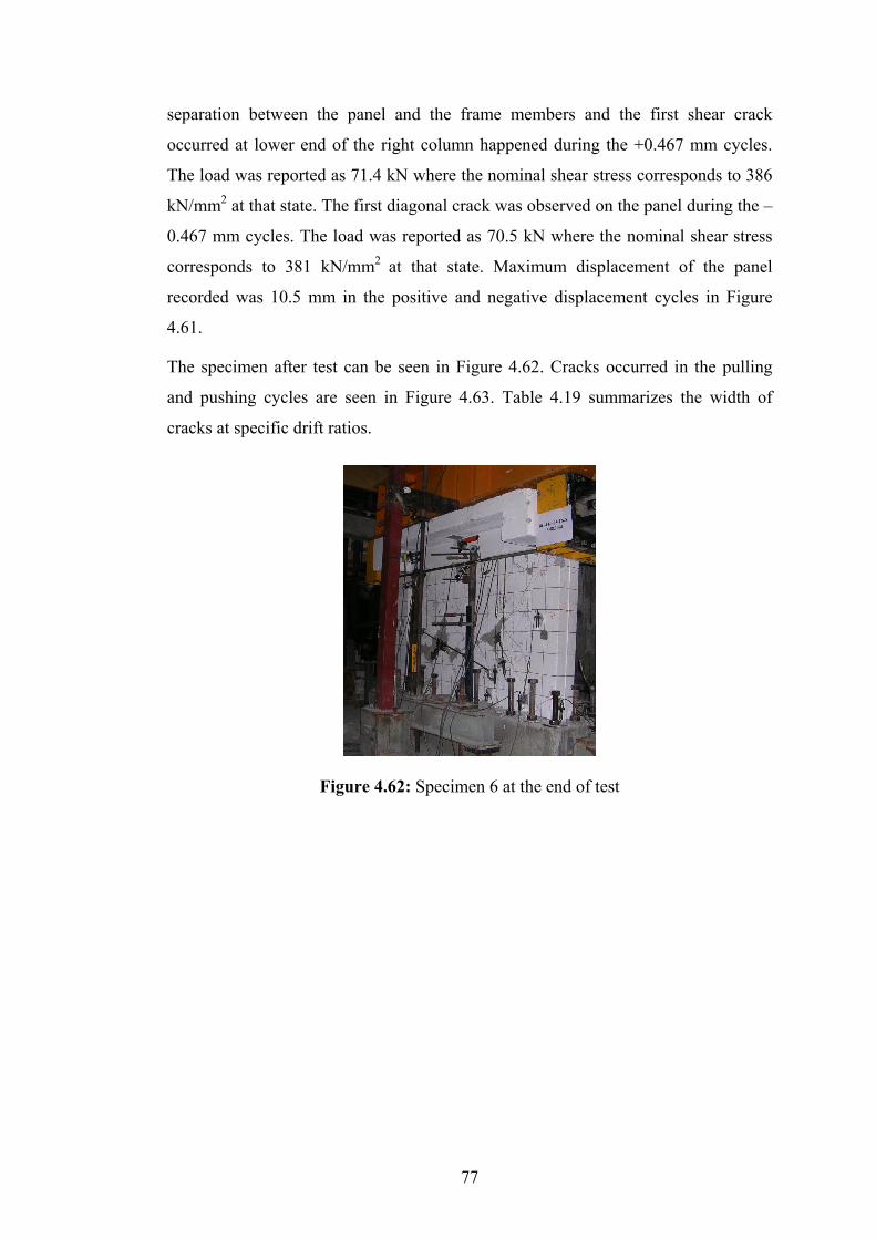
77

separation between the panel and the frame members and the first shear crack

occurred at lower end of the right column happened during the +0.467 mm cycles.

The load was reported as 71.4 kN where the nominal shear stress corresponds to 386

kN/mm2 at that state. The first diagonal crack was observed on the panel during the –

0.467 mm cycles. The load was reported as 70.5 kN where the nominal shear stress

corresponds to 381 kN/mm2 at that state. Maximum displacement of the panel

recorded was 10.5 mm in the positive and negative displacement cycles in Figure

4.61.


and pushing cycles are seen in Figure 4.63. Table 4.19 summarizes the width of



78



Crack no: Drift = 1% Drift = 2% Crack

no: Drift = 1% Drift = 2%

1 1.6 2.5 11 0.4 >3.5 2 1.6 1.6 12 1.2 1.8 3 <3.5 13 1.2 3.5 4 1.2 >3.5 14 0.8 >3.5 5 2.5 >3.5 15 0.3 2.0 6 1.2 1.2 16 1.0 <3.5 7 2.5 >3.5 17 0.7 2.0 8 0.7 >3.5 18 0.3 3.5 9 3.0 >3.5 19 - 2.5 10 0.3 <3.5 20 - 2.0








12

3

456

7

8

9

10

11 12

13

14

15

16 17

18

19

20

Push Pull

79

-56 -42 -28 -14 0 14 28 42 56-400

-300

-200

-100

0

100

200

300

400-0.04 -0.03 -0.02 -0.01 0.00 0.01 0.02 0.03 0.04

Bas

e Sh

ear

[kN

]

Displacement [mm]


Drift


bare 6



(kN) +∆ max

(mm) -P max

(kN) −∆ max

(mm) +Pult

(kN) -Pult

(kN) ∆ult

(mm)

Specimen 1 Bending + Shear failure at column ends 133 28 -123 -28.0 104 -86 42

Specimen 6 Shear failure at column ends 374 28 -359 -10.5 132 -110 28



Maksimum load [kN]




Proportion ratio


δ

80

0 10 20 30 40 500

20000

40000

60000

80000C

umul

ativ

e E

nerg

y D

issi

patio

n [k

Nm

m]

Displacement [mm]



Specimens 1 and 6

0

10000

20000

30000

40000

50000

60000

70000

0.01 0.02 0.03

Drift

Cum

ulat

ive

Ene

rgy

Diss

ip[k

Nm

m]


Cum

ulat

ive

Ene

rgy

Dis

sipa

tion

[kN

mm

]


various drifts




Table 4.22.




δ

δ

81








• The energy dissipation of the Specimen 6 at 1% story drift are 9.7 times, at 2%

story drift are 5.2 times compared to the bare frame’s shown in Figure 4.65 and

4.66.


This is the undamaged RC frame, retrofitted with shotcrete panel that is connected

only to the beams after a pre-reverse deflection applied to the beam. The types of the

LVDTs and what was measured by them for the Specimen 7 are given in Table 3.4

and Figure 3.13.




strengths in tension is 209 kN obtained at 28 mm cycles which correspond to 2%

story drift and in compression is 211 kN obtained at 10.5 mm cycles. The maximum

story drift reached is 3%. The ultimate lateral load carrying capacities of the frame

are 45 kN and 42 kN in tension and compression, respectively. The envelope curve

of the hysteretic response of the specimen is given in Figure 4.68.

82

-50 -40 -30 -20 -10 0 10 20 30 40 50-300

-200

-100

0

100

200

300

Bas

e Sh

ear

[kN

]


-56 -42 -28 -14 0 14 28 42 56-300

-200

-100

0

100

200

300-0.04 -0.03 -0.02 -0.01 0.00 0.01 0.02 0.03 0.04

Bas

e Sh

ear

[kN

]

Displacement [mm]

Drift





load at that level for Specimen 7 is 205 kN. At the bottom end of the right column

when the rotation is 0.01 radian, the corresponding load at that level for Specimen 7

is 210 kN.

δ

δ

83

-0.06 -0.04 -0.02 0.00 0.02 0.04 0.06-300

-200

-100

0

100

200

300

Bas

e Sh

ear

[kN

]

Rotation

-0.06 -0.04 -0.02 0.00 0.02 0.04 0.06-300

-200

-100

0

100

200

300

Bas

e Sh

ear

[kN

]

Rotation


-0.06 -0.04 -0.02 0.00 0.02 0.04 0.06-300

-200

-100

0

100

200

300

Bas

e Sh

ear

[kN

]

Rotation-0.06 -0.04 -0.02 0.00 0.02 0.04 0.06

-300

-200

-100

0

100

200

300

Bas

e Sh

ear

[kN

]

Rotation


-50 -40 -30 -20 -10 0 10 20 30 40 50-300

-200

-100

0

100

200

300

Bas

e Sh

ear

[kN

]

Displacement [mm]

Figure 4.71: Panel horizontal displacement at top

84

-50 -40 -30 -20 -10 0 10 20 30 40 50-300

-200

-100

0

100

200

300

Bas

e Sh

ear

[kN

]

Displacement [mm] Figure 4.72: Panel horizontal displacement at middle

-50 -40 -30 -20 -10 0 10 20 30 40 50-300

-200

-100

0

100

200

300

Bas

e Sh

ear

[kN

]

Displacement [mm]

Figure 4.73: Panel horizontal displacement at bottom

The maximum force response that has occurred at the end of the positive

displacement cycles was 209 kN and in negative displacement cycles was 211 kN.

The nominal shear stresses corresponding to these values are 1267 kN/mm2 and 1279

kN/mm2. The separation at the end of the left column occurred during the -0.7 mm

cycles. In that cycle, the load was 54 kN. The shear crack at the upper end of the

right column occurred during the +4.2 mm cycles. In that cycle, the load was 131 kN

where the nominal shear stress correspond to 794 kN/mm2. The first diagonal crack

observed on the panel occurred during the +2.8 mm cycles. In that cycle, the load

85

was 106 kN where the nominal shear stress correspond to 642 kN/mm2. Maximum

displacement of the panel recorded was 25 mm in the positive displacement cycles

and 25 mm in the negative ones can be seen in Figure 4.71. In Figure 4.72 and 4.73,

the displacements occurred at the middle and at the bottom of the wall can be seen.


and pushing cycles are seen in Figure 4.75. Table 4.23 summarizes the width of




Push Pull

1

23

4 56 7

8

9 10

86


Crack no: Drift = 1% Drift = 2% 1 1.8 3.5 2 2.0 3.5 3 1.4 0.8 4 2.5 3.5 5 3.5 >3.5 6 3.0 >3.5 7 0.7 3.5 8 2.5 >3.5 9 0.7 >3.5 10 0.3 1.4 11 2.0 >3.5 12 - 3.5 13 - 1.8 14 - 1.8








-56 -42 -28 -14 0 14 28 42 56-400

-300

-200

-100

0

100

200

300

400-0.04 -0.03 -0.02 -0.01 0.00 0.01 0.02 0.03 0.04

Bas

e Sh

ear

[kN

]

Displacement [mm]


Drift


bare 7

δ

87


name Failure mode +P max (kN)

+∆ max (mm)

-P max (kN)

−∆ max (mm)

+Pult (kN)

-Pult (kN)

∆ulti (mm)

Specimen 1 Bending + Shear failure at column ends 133 28 -123 -28.0 104 -86 42

Specimen 7 Shear failure at column ends 209 28 -211 -10.5 45 -52 42

Table 4.25: Maximum base shears recorded during the tests


0 10 20 30 40 500

20000

40000

60000

80000

Cum

ulat

ive

Ene

rgy

Dis

sipa

tion

[kN

mm

]

Displacement [mm]



Specimens 1 and 7

Maksimum load [kN]




Proportion ratio


δ

88

0

10000

20000

30000

40000

50000

60000

70000

0.01 0.02 0.03

Drift

Cum

ulat

ive

Ene

rgy

Diss

ip[k

Nm

m]


Cum

ulat

ive

Ene

rgy

Dis

sipa

tion

[kN

mm

]






Table 4.26.











• The energy dissipation of the Specimen 7 at 1% story drift are 4.3 times,

at 2% story drift are 2.6 times, at 3% story drift are 1.7 times compared to

the bare frame’s shown in Figure 4.77 and 4.78.

δ

89


This specimen is a conventional shear wall used as a reference frame and the effect

of the different strengthening methods is compared and discussed with this

specimen’s results. The types of the LVDTs and what was measured by them for

Specimen 8, are given at Table 3.3 and Figure 3.12.




strengths in tension is 329 kN obtained at 10.5 mm cycles which correspond to

0.75% story drift and in compression is 275 kN obtained at 3.5 mm cycles. The

maximum story drift reached is 1%. The ultimate lateral load carrying capacities of

the frame are 261 kN and 129 kN in tension and compression, respectively. The

envelope curve of the hysteretic response of the specimen is given in Figure 4.80.

-30 -20 -10 0 10 20 30-400

-300

-200

-100

0

100

200

300

400

Bas

e Sh

ear

[kN

]

Displacement [mm]


90

-42 -28 -14 0 14 28 42-400

-300

-200

-100

0

100

200

300

400-0.03 -0.02 -0.01 0.00 0.01 0.02 0.03

Bas

e Sh

ear

[kN

]

Displacement [mm]

Drift




the top and bottom end of the right column, the rotation didnot reach 0.01 radian like

the other specimens.

-0.04 -0.02 0.00 0.02 0.04-400-300-200-100

0100200300400

Bas

e Sh

ear

[kN

]

Rotation

-0.04 -0.02 0.00 0.02 0.04-400-300-200-100

0100200300400

Bas

e Sh

ear

[kN

]


-0.04 -0.02 0.00 0.02 0.04-400-300-200-100

0100200300400

Bas

e Sh

ear

[kN

]

Rotation

-0.04 -0.02 0.00 0.02 0.04-400-300-200-100

0100200300400

Bas

e Sh

ear

[kN

]


91

-30 -20 -10 0 10 20 30-400

-300

-200

-100

0

100

200

300

400

Bas

e Sh

ear

[kN

]

Displacement [mm]



329 kN and in negative displacement cycles was 275 kN. The nominal shear stresses

corresponding to these values are 1778 kN/mm2 and 1486 kN/mm2. The first

separation between the panel and the frame members happened during the +0.7 mm

cycles. The load was reported as 191 kN where the nominal shear stress corresponds

to 1032 kN/mm2 at that state. The first diagonal crack and the first shear crack at the

upper end of the left column was observed on the panel during the –0.467 mm

cycles. Maximum displacement of the panel recorded was 5 mm in the positive

displacement cycles and 0.4 mm in the negative ones shown in Figure 4.83.


and pushing cycles are seen in Figure 4.85. Table 4.27 shows the width of cracks at

specific drift ratios.

92




Crack no: Drift = 1% 1 >3.5 2 >3.5 3 >3.5 4 1.0 5 >3.5 6 0.9 7 >3.5 8 >3.5 9 1.2



1

2 3

4

5

6

7

8

9

Push Pull

93






-56 -42 -28 -14 0 14 28 42 56-400

-300

-200

-100

0

100

200

300

400-0.04 -0.03 -0.02 -0.01 0.00 0.01 0.02 0.03 0.04

Bas

e Sh

ear

[kN

]

Displacement [mm]


Drift


bare 8



(kN) +∆ max

(mm) -P max

(kN) −∆ max

(mm) +Pult

(kN) -Pult

(kN) ∆ult

(mm)


Specimen 8 Shear failure at column ends 329 10.5 -275 -3.5 261 -129 14



Maksimum load [kN]




Proportion ratio


94

0 10 20 30 40 500

20000

40000

60000

80000C

umul

ativ

e E

nerg

y D

issi

patio

n [k

Nm

m]

Displacement [mm]



Specimens 1 and 8

0

10000

20000

30000

40000

50000

60000

70000

0.01 0.02 0.03

Drift

Cum

ulat

ive

Ene

rgy

Diss

ip[k

Nm

m]


Cum

ulat

ive

Ene

rgy

Dis

sipa

tion

[kN

mm

]






Table 4.30.

95




• Comparison of Figures 4.81 and 4.82 with Figures 4.4 and 4.5; at the top and

bottom end of the right column, the rotation did not reach 0.01 radian like the

other specimens.

• The energy dissipation of the Specimen 8 at 1% story drift is 10.8 times

compared to the bare frame’s shown in Figure 4.87 and 4.88.

4.11 Evaluation of the Test Results

The comparison of results of the six test specimens with shotcrete panel and one

shear wall specimen to the bare frame (Specimen 1) and within each other are

explained briefly below. Each specimen is evaluated according to the parameters

stated in Table 3.1. Failure modes, load carrying capacities, initial stiffnesses, energy

dissipation capacities and lateral stiffnesses are discussed here.

4.11.1 Failure modes

Table 4.31 summarizes the maximum loads, the ultimate loads frames carried in pull

and push cycles and the failure modes occurred. These data are taken from the

experimental study. As can be seen in the table; bending and shear failure at column

ends occurred in the bare frame, while generally shear failure at column ends

observed in the retrofitted frames. This is because the specimens have low shear

strength properties to represent the building stock of Turkey. No matter how strong

wet-mixed sprayed concrete panels were, the ultimate failure mode of the systems

were controlled by the existing shear capacity of the outer frames. All of the

strengthened frame experiments were ended due to severe shear cracks occurring at

the end of the columns.

On the web of short beams which exist on the right and left side of the panel in the

case of partially infilled specimen, some 0.2 mm-width shear cracks are observed.

The cracks are seen first at 0.2% story drift. At the end of the tests, the width of these

cracks increased to 0.5 mm. However these kinds of cracks are not observed at the

same region of the fully infilled specimens.

96

Table 4.31: Effect of retrofitting on general quantities

Specimen

Type Failure m

ode +P

max

(kN)

+∆ m

ax (m

m)

-P m

ax (kN

) −∆

max

(mm

) +P

ult (kN

) -P

ult (kN

) ∆

ult (m

m)

1

B

ending + Shear failure at column ends

133.0 28.0

-123.0 -28.0

104.0 -86.0

42.0

3

Shear failure at column ends

291.0 10.5

-279.0 -10.5

165.0 -136.0

14.0

5

Shear failure at colum

n ends 217.0

28.0 -207.0

-28.0 77.0

-89.0 42.0

6 δ


n ends 374.0

28.0 -359.0

-10.5 132.0

-110.0 28.0

7

δ


n ends 209.0

28.0 -211.0

-10.5 45.0

-52.0 42.0

2S

Shear failure at column ends

342.0 28.0

-394.0 -28.0

166.0 -249.0

28.0

4S


n ends 236.0

28.0 -190.0

-28.0 120.0

-118.0 42.0

8


n ends 329.0

10.5 -275.0

-3.5 261.0

-129.0 14.0

97

4.11.2 Lateral load carrying capacity

Table 4.32 summarizes the maximum loads carried by the retrofitted RC frames in

push and pull cycles. The lateral load carrying capacity increases are also calculated

and presented in proportion ratios compared with that of the bare frame’s.


Maximum load [kN] Ratio to Specimen 1 Specimen Push Pull Push Pull

1 133 -123 1.0 1.0 3 291 -279 2.2 2.3 5 217 -207 1.6 1.7 6 374 -359 2.8 2.9 7 209 -211 1.6 1.7 2S 342 -394 2.6 3.2 4S 236 -190 1.8 1.5 8 329 -275 2.5 2.2

The lateral load carrying capacity increased between 2.2 to 3.2 times for the

specimens with shotcrete panel that were fully connected to the frame, and between

1.6 to 1.8 times for the specimens with shotcrete panel with a gap between the panel

and the columns compared with the bare frame’s. Because the frames were pre-

damaged, the capacity differences between push and pull cycles both for Specimen

2S and 4S has occurred. The specimen with the shear wall shows the same amount of

increase with the fully connected shotcrete panel ones. Pre-reverse deflection seems

to make a 30% increase in the lateral load carrying capacity of the specimen for the

specimens with shotcrete panel fully connected to the frame and no significant effect

on the specimens which have shotcrete panels that are connected only to the beams.

The comparison of the envelope curves of the hysteretic responses of the two fully

connected shotcrete panel specimens to the bare frame’s are given in Figure 4.89.

98

-56 -42 -28 -14 0 14 28 42 56-400

-300

-200

-100

0

100

200

300

400-0.04 -0.03 -0.02 -0.01 0.00 0.01 0.02 0.03 0.04

Bas

e Sh

ear

[kN

]

Displacement [mm]

Specimen 1 Specimen 3 Specimen 2S

Drift

Figure 4.89: The comparison of envelope curves of Specimens 1, 2S and 3

Although Specimen 2S was a representative of a damaged frame, its performance

was higher than Specimen 3. It is attributed to the higher compressive strength of

outer frame and wet-mixed sprayed concrete panel. For this reason in Figure 4.90,

the analytical solution of Specimen 3 with using the frame and the shotcrete panel

concrete compressive strength of Specimen 2S, named as “analytical 3_2S”, are

sketched with Specimen 2S and 3.

-56 -42 -28 -14 0 14 28 42 56-400

-300

-200

-100

0

100

200

300

400-0.04 -0.03 -0.02 -0.01 0.00 0.01 0.02 0.03 0.04

Bas

e Sh

ear

[kN

]

Displacement [mm]

Specimen 2S Analytical 3_2S Specimen 3

Drift

Figure 4.90: The comparison of envelope curves of Specimens 2S and 3 with

analytical 3_2S

99

The two shotcrete specimens, which are connected only to the beams, are given in

Figure 4.91.

-56 -42 -28 -14 0 14 28 42 56-400

-300

-200

-100

0

100

200

300

400-0.04 -0.03 -0.02 -0.01 0.00 0.01 0.02 0.03 0.04


Bas

e Sh

ear

[kN

]

Displacement [mm]

Drift

Figure 4.91: The comparison of envelope curves of Specimens 1, 4S and 5

The pre-reverse effect on the load carrying capacities can be seen in Figure 4.92 for

fully connected shotcrete panel specimens. Since the concrete compressive strengths

of Specimen 3 and 6 are not the same, Specimen 3’s behaviour is predicted

analytically using Specimen 6’s concrete strengths, named as “analytical 3_6”, and

introduced as an envelope curve in Figure 4.93. In Figure 4.94 for shotcrete

specimens, which are connected only to the beams are presented. In Figure 4.95 only

the pre-reversed beam specimens are compared within each other.

100

-56 -42 -28 -14 0 14 28 42 56-400

-300

-200

-100

0

100

200

300

400-0.04 -0.03 -0.02 -0.01 0.00 0.01 0.02 0.03 0.04

Bas

e Sh

ear

[kN

]

Displacement [mm]

Specimen 1 Specimen 6 Specimen 3

Drift

Figure 4.92: The comparison of envelope curves of Specimens 1, 3 and 6

-56 -42 -28 -14 0 14 28 42 56-400

-300

-200

-100

0

100

200

300

400-0.04 -0.03 -0.02 -0.01 0.00 0.01 0.02 0.03 0.04

Bas

e Sh

ear

[kN

]

Displacement [mm]

Specimen 6 Analytical 3_6 Specimen 3

Drift

Figure 4.93: The comparison of envelope curves of Specimens 3 and 6 with analytical 3_6

δ

101

-56 -42 -28 -14 0 14 28 42 56-400

-300

-200

-100

0

100

200

300

400-0.04 -0.03 -0.02 -0.01 0.00 0.01 0.02 0.03 0.04

Bas

e Sh

ear

[kN

]

Displacement [mm]


Drift


-56 -42 -28 -14 0 14 28 42 56-400

-300

-200

-100

0

100

200

300

400-0.04 -0.03 -0.02 -0.01 0.00 0.01 0.02 0.03 0.04


Bas

e Sh

ear

[kN

]

Displacement [mm]

Drift


The comparison of shotcrete walls with the shear wall (Specimen 8) is given in

Figure 4.96. Since the concrete compressive strengths of Specimen 1, 3 and 8 are not

the same, Specimen 1 and 3’s behaviours are predicted analytically using Specimen

8’s concrete strengths and introduced as envelope curves in Figure 4.97.

δ

δ

δ

102

-56 -42 -28 -14 0 14 28 42 56-400

-300

-200

-100

0

100

200

300

400-0.04 -0.03 -0.02 -0.01 0.00 0.01 0.02 0.03 0.04

Specimen 1 Specimen 8 Specimen 5 Specimen 3

Bas

e Sh

ear

[kN

]

Displacement [mm]

Drift

Figure 4.96: The comparison of envelope curves of Specimens 1, 3, 5 and 8

-56 -42 -28 -14 0 14 28 42 56-400

-300

-200

-100

0

100

200

300

400-0.04 -0.03 -0.02 -0.01 0.00 0.01 0.02 0.03 0.04

Analyical Bare 1_8 Specimen 8 Specimen 5 Analytical 3_8

Bas

e Sh

ear

[kN

]

Displacement [mm]

Drift

Figure 4.97: The comparison of envelope curves of Specimens 1, 3, 5 and 8 with

analytical 3_8 and analytical 1_8

4.11.3 Initial stiffness

Table 4.33 compares the initial stiffness of the eight specimens in this study and the

increases given as proportion ratios to that of the bare frame’s are also presented. The

initial stiffness values are calculated as the slope of the line joining the points of the

maximum loads in push and pull cycle occurred during initial stages.

103


The damaged and undamaged frames strengthened in this study yield the following

results: The lateral stiffness of the frames right before the first cracks occurred in the

system increased by 10 times for the damaged frames Specimen 2S and 4S, and 8.5

times for undamaged frames Specimen 3 and 5 compared with the bare frame’s. The

pre-reversed shotcrete panel specimens also showed almost the same amount of

increase in stiffness while the shear wall has increased the stiffness of the frame 20

times.

In Figure 4.98 initial stiffness of the specimens are compared in graphic format.

0

100

200

300

400

500

Initi

al S

tiffn

ess [

kN/m

m]

Specimen 1Specimen 3Specimen 5Specimen 6Specimen 7Specimen 2SSpecimen 4SSpecimen 8

Figure 4.98: Initial stiffnesses of the specimens

4.11.4 Cumulative energy dissipation

As shown in Figure 4.99, the cumulative energy dissipation of the specimens with

shotcrete walls that are fully connected to the frame; are 10 and 5 times higher than

the bare frame’s at 1% and 2% story drift, respectively. For the specimens with gaps;

cumulative energy dissipation values are 4, 2.5 and 1.7 times higher than the bare

Specimen Initial stiffness [kN/mm]

Ratio to Specimen 1

1 21.6 1.0 3 183.9 8.5 5 188.5 8.7 6 249.9 11.6 7 179.3 8.3 2S 230.9 10.7 4S 223.3 10.3 8 444.0 20.5

104

frame’s at 1%, 2% and 3% story drift, respectively. The specimen with the shear wall

shows the same amount of energy dissipation with the fully connected shotcrete

panel one and could only make 1% story drift.

0

10000

20000

30000

40000

50000

60000

70000

1 2 3

Drift

Cum

ulat

ive

Ene

rgy

Diss

ipat

ion

[k

Specimen 1Specimen 3Specimen 5Specimen 6Specimen 7Specimen 2SSpecimen 4SSpecimen 8

Figure 4.99: Cumulative energy dissipation capacities at various story drifts

The comparison of the cumulative energy dissipation capacities of the two fully

connected shotcrete panel specimens to the bare frame’s are given in Figure 4.100

and for the two shotcrete specimens, which are connected only to the beams are

given in Figure 4.101.

0 10 20 30 40 500

20000

40000

60000

80000

Cum

ulat

ive

Ene

rgy

Dis

sipa

tion

[kN

mm

]

Displacement [mm]



Specimens 1, 2S and 3

% % %

105

0 10 20 30 40 500

20000

40000

60000

80000

Cum

ulat

ive

Ene

rgy

Dis

sipa

tion

[kN

mm

]

Displacement [mm]



Specimens 1, 4S and 5

The pre-reverse effect on the load carrying capacities can be seen in Figure 4.102 for

fully connected shotcrete panel specimens and in Figure 4.103 for shotcrete

specimens, which are connected only to the beams, with and without pre-reverse of

the beam and in Figure 4.104 only the results of pre-reversed beam specimens are

given.

0 10 20 30 40 500

20000

40000

60000

80000

Cum

ulat

ive

Ene

rgy

Dis

sipa

tion

[kN

mm

]

Displacement [mm]



Specimens 1, 3 and 6

δ

106

0 10 20 30 40 500

20000

40000

60000

80000C

umul

ativ

e E

nerg

y D

issi

patio

n [k

Nm

m]

Displacement [mm]




0 10 20 30 40 500

20000

40000

60000

80000

Cum

ulat

ive

Ene

rgy

Dis

sipa

tion

[kN

mm

]

Displacement [mm]




The comparison of shotcrete walls with the shear wall is given in Figure 4.105.

δ

δ

δ

107

0 10 20 30 40 500

20000

40000

60000

80000

Cum

ulat

ive

Ene

rgy

Dis

sipa

tion

[kN

mm

]

Displacement [mm]



Specimens 1, 3, 5 and 8

4.11.5 Equivalent damping characteristics

Hysteretic damping, ξhysteretic, has been determined for the specimens through the

hysteresis lateral load-top displacement curves. Paying attention on the stabilized

loops, some average equivalent viscous damping ratios which can be used in the

rehabilitation design stage of existing structures were obtained.

The lower and upper limits suggested above have been calculated through the

formula which is given in Equation 4.3.

Deq hysteretic

S

W0.05 0.05

4 Wξ = + βξ = + β×

π

(4.3)

where β is a coefficient between 0.33–1.0 in FEMA 273 (1997) and WD and WS are

indicating the energy dissipated in one cycle of preferably stabilized displacement

and the strain energy at the corresponding displacement given in Figure 4.106 as

Priestley et al., 2007 suggessted.

108

Figure 4.106: Dissipated and strain energy

The constant value of 0.05 in Eq. 4.3 represents the viscous damping of reinforced

concrete building inherently exist in the structure and ξhysteretic can be taken

approximately as 10% of critical damping depending on the tests results summarized

and the diagrams that are given in Figure 4.107. One can easily find by the

corresponding factors for these damping ratios to define the redesign demand curves

referring the standard one, which may have some minor differences from source to

source, FEMA 273, 1997, NEHRP, 2000.

0.00

0.05

0.10

0.15

0.20

0 10 20 30 40 50

Displacement (mm)

Perc

enta

ge o

f Cri

tical

Dam

without pre-reverse deflectionbare framewith pre-reverse deflectionLi ( ih d fl i )

Figure 4.107: Equivalent damping for various tests

It can be concluded that the damping ratio can definitely be taken as higher than 5%

of critical damping which is being suggested by current codes, TEC 1997 and 2007.

The suggested equivalent viscous damping for rehabilitation design stage is between

Force

Displacem ent

W D

W S

S

Dhysteretic W

Wπ

ξ4

=

1% 2% 3%

Story Drift

109

8-16% of critical damping depending on the type of modification. At 1% story drift,

the observed percentage of critical damping values are 10.5% and 13.5% for without

and with pre-reverse deflection on the beam, respectively

4.11.6 Lateral stiffness

The comparison of the lateral stiffness of the two fully connected shotcrete panel

specimens to the bare frame’s are given in Figure 4.108 and for the two shotcrete

specimens, which are connected only to the beams are given in Figure 4.109.

0.00 0.01 0.02 0.030

100

200

300

400

Lat

eral

Stif

fnes

s [kN

/mm

]

Drift


Figure 4.108: The comparison of lateral stiffnesses of Specimens 1, 2S and 3

0.00 0.01 0.02 0.030

100

200

300

400

Lat

eral

Stif

fnes

s [kN

/mm

]

Drift

Specimen 1 Specimen 4S Specimen 5

Figure 4.109: The comparison of lateral stiffnesses of Specimens 1, 4S and 5

110

The pre-reverse effect on stiffness can be seen in Figure 4.110 for fully connected

shotcrete panel specimens and in Figure 4.111 for shotcrete specimens, which are

connected only to the beams, with and without pre-reverse of the beam and in Figure

4.112 only the results of pre-reversed beam specimens are given.

0.00 0.01 0.02 0.030

100

200

300

400

Lat

eral

Stif

fnes

s [kN

/mm

]

Drift


Figure 4.110: The comparison of lateral stiffnesses of Specimens 1, 3 and 6

0.00 0.01 0.02 0.030

100

200

300

400

Lat

eral

Stif

fnes

s [kN

/mm

]

Drift



δ

δ

111

0.00 0.01 0.02 0.030

100

200

300

400

Lat

eral

Stif

fnes

s [kN

/mm

]

Drift



The comparison of shotcrete walls with the shear wall is given in Figure 4.113.

0.0000 0.0025 0.0050 0.0075 0.01000

200

400

600

800

1000

Lat

eral

Stif

fnes

s [kN

/mm

]

Drift


Figure 4.113: The comparison of lateral stiffnesses of Specimens 1, 3, 5 and 8

The lateral stiffness is almost the same for all the test specimens after 1% drift ratio.

The pre-reverse is not very effective on the stiffnesses.

δ

δ

112

4.11.7 Rotation of the panels

The panel base rotations of Specimens were obtained using the measuring system

given in Figure 4.114. In the figure; ∆1 and ∆2 correspond to the measured shortening

and elongation of the related cross section, while x is the distance between them.

The rotation is calculated using Equation 4.4;

θ = (∆1+∆2) / x (4.4)

∆1 ∆2

x

after deformation

before deformation

Figure 4.114: Calculation of rotation of the shotcrete panel

Base rotation of the shotcrete panel versus base shear relations are given for

Specimens 3, 5 and 8 in Figures 4.115, 4.116 and 4.117, respectively. The graphs are

drawn and compared for 1% story drift. From the figures, it can easily be concluded

that the response of Specimens 3 and 8 are similar and linear elastic. However in the

case of Specimen 5, stable hysteretic loops were observed.

For the 1% story drift level, in Specimens 3 and 8 rotation amplitudes are relatively

small, while in Specimen 5 the amplitude of the rotation is relatively higher

compared to the others and response shows inelastic excursion.

113

-0.010 -0.005 0.000 0.005 0.010-400

-300

-200

-100

0

100

200

300

400

Bas

e Sh

ear

[kN

]

Strain Figure 4.115: The rotation of the panel for Specimen 3

-0.010 -0.005 0.000 0.005 0.010-300

-200

-100

0

100

200

300

Bas

e Sh

ear

[kN

]

Rotation

Figure 4.116: The rotation of the panel for Specimen 5

114

-0.010 -0.005 0.000 0.005 0.010-400

-300

-200

-100

0

100

200

300

400

Bas

e Sh

ear

[kN

]

Displacement [mm] Figure 4.117: The rotation of the panel for Specimen 8

115

5. ANALYTICAL STUDIES USING THE FINITE ELEMENT METHOD

There are several suggested numerical models to represent the effect of the infill

walls on the behaviour of the infilled frames which are adapted in several computer

programs. ANSYS, ABAQUS, DIANA, SAP2000, OpenSees, IDARC, SeismoStruct

are some of these programs. In this study, the overall effect of the shotcrete wall on

the system behavior is investigated. For this reason, SeismoStruct which has a macro

approach for the problem considered is preferred. SeismoStruct models the infill wall

with some diagonal braces which is a new approach that gives the opportunity to

obtain a more acceptable result compared with the experimental studies, (Crisafulli,

1997).

This chapter presents detailed information about the program used to model the

experiments tested during the course of this research analytically. The analyses were

carried out to predict the load versus drift relations and the failure modes of the

specimens. Smyrou et al. (2006), Casarotti and Pinho (2007), Pinho et al. (2007),

Cattari and Lagomarsino (2006), Mellal et al. (2003), Kutanis et al. (2007), Crowley

and Pinho (2006), Negulescu et al. (2003), Nogueiro et al. (2003), Calvi et al. (2006),

Priestley et al. (2007) have studied SeismoStruct and have achieved success in

modelling analytically reinforced concrete and steel structure behaviour.

In SeismoStruct, the diagonal braces representing the infill wall and the parameters

for defining these braces are designed originally for modelling the brick walls. The

model is developed by Crisafulli (1997) and adopted to SeismoStruct by Blandon

(2005). In this model, the hysteretic behaviour of masonry in compression is defined

by Sargin’s (1971) equation which is originally proposed for concrete. The behaviour

in tension is assumed to be linear. Since there is not sufficient experimental data

related to the cyclic axial behaviour of masonry, Crisafulli used experimental data

obtained from concrete specimens to calibrate the model. He also tested concrete

specimens under cyclic compression to obtain experimental data and used these

results to calibrate the analytical model of inner loops of the hysteretic behaviour in

compression.

116

In this study, the parameters of the diagonal braces which are used to model the

shotcrete panel are taken from the material tests which were presented in Chapter 3.

While deciding on these parameters, several, necessary discussions have been done

with the developer of SeismoStruct, namely Assist.Prof.Dr. Rui Pinho (2006). Since

global response is aimed in this study rather than the local effects of the infill wall,

by correct calibration of the parameters, the analysis can be valid.

One of the advantages of SeismoStruct is that the interaction between the wall and

the surrounding frame can be modelled by defining extra nodes both in the beam and

the columns.

5.1 Nonlinear Static Analysis Using SeismoStruct

Inelastic beam-column elements are used in the program. To allow more accurate

evaluation of structural damage distribution, material inelasticity is assumed to

spread along the member length and across the cross section. This is explicitly

represented by implementing a fibre modelling approach as shown in Figure 5.1.

Figure 5.1: Fibre analysis approach

The loading pattern of the experiments is applied in static time-history analysis. In

static time-history analysis, the applied loads (displacement, force or a combination

of both) can vary independently in the pseudo-time domain, according to a

prescribed load pattern. The applied load Pi in a nodal position i is given by

Pi = li(t) Pi0, i.e. a function of the time-dependent load factor li(t) and the nominal

load Pi0. This type of analysis is typically used to model static testing of structures

subjected to various force or displacement patterns.

In the finite element analysis of the tested specimens that are the single story, single

bay RC frames infilled with shotcrete panels, strut modelling is used.

117

5.2 Description of Element Types Used

Inelastic frame elements were used for modelling the RC frame. These are the 3D

beam-column elements capable of modelling members of space frames having

geometric and material nonlinearities. The sectional stress-strain state of beam-

column elements is obtained through the integration of the nonlinear uniaxial

material response of the individual fibres in which the section has been subdivided.

Local geometric nonlinearity (beam-column effects) is also comprised within the

formulation of this element.

If a sufficient number of fibres (200-400 in spatial analysis) are employed, the

distribution of material nonlinearity across the section area is accurately modelled,

even in the highly inelastic range. Two integration Gauss points as shown in Figure

5.2 per element are then used for the numerical integration of the governing

equations of the cubic formulation. If a sufficient number of elements are used such

as 5-6 per structural member, the spread of inelasticity along member length can be

accurately estimated.

Figure 5.2: Gauss integration points in beam column elements

5.3 Material Models

Some of the defined parameters which are used in the material models are taken from

the tests done to get the characteristic values of the materials. The average values of

several tests are used both for concrete and reinforcement. For those parameters

which cannot be determined from the tests, these values are taken from the interval

given in the manual of the program itself.

118

5.3.1 Material model used for steel reinforcement

Monti-Nutti steel model is used to model the reinforcement in the frame. It is a

uniaxial steel model initially programmed by Monti et al. (1996). It uses the

Menegotto and Pinto (1973) stress-strain relationship together with the isotropic

hardening rules proposed by Filippou et al. (1983). An additional memory rule

proposed by Fragiadakis (2001) is also introduced, for higher numerical

stability/accuracy under transient seismic loading.

Eleven model-calibrating parameters summarised in Table 5.1 must be defined in

order to fully describe the mechanical characteristics of steel reinforcement.

Table 5.1: Input parameters for steel reinforcement

Parameter Definition Es Modulus of elasticity fy Yield strength µ Strain hardening parameter R0 Transition curve initial shape parameter a1 Transition curve shape calibrating coefficients a2 Transition curve shape calibrating coefficients P Kinematic/isotropic weighing coefficient r Spurious unloading corrective parameter L Transverse reinforcement spacing D Longitudinal bar diameter γ Specific weight

These are:

1- Modulus of elasticity – Es: This is the initial elastic stiffness of the material. The

value is taken from Table 3.10 which summarises the material test results.

2- Yield strength – fy: This is the stress at yield. The value is taken from Table 3.10.

3- Strain hardening parameter - µ: This is the ratio between the post-yield stiffness

(Esp) and the initial elastic stiffness (Es) of the material. The former is defined as

Esp=(fult - fy)/(εult - fy/Es), where fult and εult represent the ultimate or maximum

stress and strain capacity of the material, respectively. This value is calculated

from the reinforcement material test results.

4- Transition curve initial shape parameter - R0: This is the initial (first loading

cycle) value of the parameter R, that controls the shape of the transition curve

between initial and post-yield stiffness, necessary to accurately represent

119

Baushinger effects and pinching of the hysteretic loops. The default value is 20.

The default value is taken into account during the analysis.

5- Transition curve shape calibrating coefficients - a1 & a2: These are the two

coefficients used to calibrate the changes that must be applied to parameter R0 in

order to obtain the updated transition curve shape parameter Rn. Whilst a1 is

usually adopted with an invariable value of 18.5, a2 might range between 0.05 and

0.15. The default values are 18.5 and 0.15 for coefficients a1 and a2, respectively.

The default value is taken into account for a1 and 0.05 for a2 during the analysis.

6- Kinematic/isotropic weighing coefficient – P: This is the weighing coefficient

used in this model to define the degree to which kinematic and isotropic hardening

are introduced in the stress-strain cyclic response characteristics of the material. A

value close to unity implies a kinematic-dominated hardening behaviour, whilst a

value close to zero is employed when isotropic hardening controls the response of

the material. P is taken as 0.9 during the analysis.

7- Spurious unloading corrective parameter – r: This is the threshold for small

strain reversals, defined as a percentage of the strain measured at the end of a

loading cycle, used to prevent the occurrence of spurious strain unloading cycles.

Typical values of r vary between 2.5 and 5 percent. r is taken as 2.5% during the

analysis.

8- Transverse reinforcement spacing and longitudinal bar diameter - L & D: These

two parameters are required for the definition of the slenderness ratio (L/D) of the

longitudinal reinforcement which in turn is used to calibrate the buckling

behaviour of this steel model. L is the spacing between the transverse

reinforcement and D is the diameter of the longitudinal bars. L is 200 mm and D is

16 mm as shown in Figure 3.4.

9- Specific weight – γ: This is the specific weight of the material.

Es, fy, µ, L and D are taken from the material test results for the reinforcement given

in detail in Chapter 3, while R0, a1, a2, P and r are predicted from the test results.

5.3.2 Material model used for concrete

Nonlinear constant confinement concrete model is used to model the concrete

surrounded by stirrups. This is a uniaxial nonlinear constant confinement model,

120

initially programmed by Madas (1993) that follows the constitutive relationship

proposed by Mander et al. (1988) and the cyclic rules proposed by Martinez-Rueda

and Elnashai (1997). The confinement effects provided by the lateral transverse

reinforcement are incorporated through the rules proposed by Mander et al. (1988)

whereby constant confining pressure is assumed throughout the entire stress-strain

range.

Five model-calibrating parameters summarised in Table 5.2 must be defined in order

to fully describe the mechanical characteristics of confined concrete:

Table 5.2: Input parameters for concrete

Parameter Definition fc Compressive strength ft Tensile strength εc Strain at peak stress kc Confinement factor γ Specific weight

These are:

1- Compressive strength – fc: This is the cylinder compressive strength of the

material. The value is taken from Table 3.8 which summarises the material test

results for frame concrete.

2- Tensile strength – ft: This is the tensile strength capacity of the material. Usually it

can be estimated as ft= kt(fc)1/2, where kt varies from 0.5 (concrete in direct tension)

to 0.75 (concrete in flexural tension), as suggested by Priestley et al. (1996). When

this value is reached, the concrete is assumed to abruptly lose its tensile resistance,

without any sort of tension softening. This values is taken as 0.1*fc.

3- Strain at peak stress - εc: This is the strain corresponding to the point of

unconfined peak compressive strength, fc. This value is taken from the material test

result of frame concrete.

4- Confinement factor – kc: This is the constant confinement factor, defined as the

ratio between the confined and unconfined compressive stress of the concrete, and

used to scale up the stress-strain relationship throughout the entire strain range. Since

the unconfined compressive stress of the concrete is known, the confined

compressive stress of the concrete is calculated from equation proposed by Mander

et al. (1988).

121

5- Specific weight - γ: This is the specific weight of the material.

fc, ft and εc are taken from the material test results conducted for concrete given in

detail in Chapter 3.

5.4 Inelastic Infill Panel Element

The effect of infill materials on the overall structural behavior of infilled frames was

investigated previously by many researchers. There are mainly two approaches to

model infilled frames. In the first approach the infill panel is modelled by plane

stress, shell elements which are interconnected at their nodes using a series of

nonlinear springs and struts to represent the shear and normal stresses interaction

between the blocks along the mortar head and bed joints. In the second approach, the

infill wall is modelled by diagonal struts with equivalent properties determined from

experimental tests. Several variations of the diagonal strut modelling have been

proposed including the use of multiple struts or truss-shaped struts in lieu of a single

strut, nonlinear properties, varying effective areas throughout the loading history and

the use of actual load-deflection paths.

Inelastic infill panel element is a four-node masonry panel element developed and

initially programmed by Crisafulli (1997) and implemented in SeismoStruct by

Blandon (2005), for the modelling of the nonlinear response of infill panels in

framed structures. Each panel is represented by six strut members; each diagonal

direction features two parallel struts to carry axial loads across two opposite diagonal

corners and a third and a fourth one to carry the shear from the top to the bottom of

the panel. This latter strut only acts across the diagonal that is on compression; hence

its "activation" depends on the deformation of the panel. The axial load struts use the

masonry strut hysteretic model, while the shear strut uses a dedicated bilinear

hysteretic rule.

Four internal nodes are employed to account for the actual points of contact between

the frame and the infill panel (i.e. to account for the width and height of the columns

and beams, respectively), whilst four dummy nodes are introduced with the objective

of accounting for the contact length between the frame and the infill panel as can be

seen in Figure 5.3. These dummy nodes with 2 translational degrees of freedom per

node are required to define one end of the strut members, which is not connected to

122

the corners of the panel. All the internal forces are transformed to the exterior four

nodes.

Figure 5.3: Strut model used

In order to fully characterise this type of element, the following parameters need to

be defined:

- Strut Curve Parameters, employed in the definition of the masonry strut hysteretic

model as shown in Figure 5.4, which is modelled with the infill panel strut response

curve.

Figure 5.4: General characteristics of the proposed model for cyclic axial behaviour of infill wall, Crisafulli (1997)

The model which defines the cyclic axial behaviour of the wall is composed by five

hysteretic rules which are:

• Envelope curve in compression (Rule 1)

123

• Unloading from the envelope curve (Rule 2)

• No stress (Rule 3)

• Reloading after complete unloading (Rule 4 and 5)

• Unloading and reloading from inside loops (small hysteretic cycle)

These rules are explained in detail in Crisafulli (1997).

Input parameters needed for the infill model are summarized in Table 5.3. Below,

these will be explained in detail.

Table 5.3: Input parameters for the infill model

Parameter Definition Em Initial young's modulus fmθ Compressive strength ft Tensile strength εm Strain at maximum stress εult Ultimate strain εcl Closing strain ε1 Strain of initial reduction of area for the strut ε2 Strain for the residual of strut's area γun Factor to calculate Eun (unloading stiffness) αre Strain reloading factor αch Factor to calculate uch βa Factor to calculate upl βch Factor to calculate fch γplu Factor to calculate eplui, eplu γplr Factor to calculate eplr ex1 Exponent to calculate eplu ex2 Exponent to calculate fch

Seventeen parameters are needed in order to fully characterise this response curve.

These are:

1- Initial Young modulus – Em: The elastic modulus represents the initial slope of

the stress-strain curve. It is related to the compressive strength of the material

(fmθ), and the values can range: 400fmθ<Em<1000fmθ, as summarised in Crisafulli

(1997). Em is taken as approximately as 1000fmθ in the analysis. Since the wall is

reinforced concrete, the maximum limit value for Em is taken.

2- Compressive strength - fmθ: This compressive strength refers to the diagonal

capacity of the infill panel, that is, it refers to the capacity of the masonry in the

direction of the principal stress f1, which, typically, is assumed to coincide with

124

the diagonal that links two opposite corner. If no diagonal compression test

results are available, then the resistance of the masonry in the normal direction fn,

is defined by adapting the failure theory proposed by Mann and Müller (1982),

Crisafulli (1997) whom developed the following equation: fmθ = fn / sin2θ. The

value is taken from Table 3.9 which summarises the material test results for

shotcrete concrete.

3- Tensile strength – ft: The tensile strength represents the tensile strength of the

masonry or the bond-strength of the interface between frame and infill panel. ft is

taken as 0.01 for the analysis.

4- Strain at maximum stress -εm: This parameter represents the strain at maximum

stress and influences, via the modification of the secant stiffness, the ascending

branch of the stress-strain curve. This value is taken from the material test result

of shotcrete concrete.

5- Ultimate strain -εult: This strain is used to control the descending branch of the

stress-strain curve, modelled with a parabola so as to obtain better control of the

strut's response (Crisafulli, 1997). For relative large values, the decrease of the

compressive strength becomes smoother and the analyses more stable. This value

is taken from the material test result of shotcrete concrete.

6- Closing strain -εcl: This parameter defines the strain after which the cracks

partially close allowing compression stresses to develop. Its values may vary

between 0 and 0.003, as suggested by Crisafulli (1997). εcl is taken as 0.003 for

Specimen 3, 6, 5 and 7 during the analysis.

7- Strut area reduction strain and Residual strut area strain -ε1 and ε2: These are

the two strains associated to the reduction of the strut area. These parameters are

difficult to find experimental supporting evidence for considering the empirical

nature of the strut area reduction scheme. Reasonable values of ε1 may be in the

range of 0.0003 to 0.0008 whilst for ε2 values in between 0.0006 and 0.016 may

be considered. ε1 and ε2 are taken as 0.004 and 0.005 for Specimen 3, 0.01 and

0.02 for Specimen 6, 0.05 and 0.07 for Specimen 5 and 0.01 and 0.02 for

Specimen 7 during the analysis, respectively.

125

8- Empirical parameters: The masonry infill strut model requires nine empirical

curve-calibrating factors to be defined, as proposed by Crisafulli (1997). Table

5.4 summarizes the suggested and limit values for these parameters.

- starting unloading stiffness factor (γun), is used to define the starting unloading

stiffness modulus as a proportion of its loading counterpart. Its value may

typically vary between 1.5 and 2.5 (though any value above unity constitutes a

valid entry). γun is taken as 1.7 for Specimen 3 and 6, 1.5 for Specimen 5 and 7

during the analysis.

- strain reloading factor (αre), is employed to predict the strain at which the loop

reaches the envelope after unloading. Its typical value ranges from 0.2 and 0.4

(though any value above zero constitutes a valid entry). αre is taken as 0.2 for


- strain inflection factor (αch), utilised in the computation of the strain at which

the reloading curve should feature an inflection point, effectively controlling, in

this way, the loops’ fatness. Its value may be found within the interval of 0.1 to

0.7. αch is taken as 0.35 for Specimen 3 and 6, 0.3 for Specimen 5 and 7 during

the analysis.

- complete unloading strain factor (βa), used in the definition of the plastic

deformation after complete unloading. Its values typically range between 1.5 and

2.0 (though any value above zero constitutes a valid entry). βa is taken as 2 for


- stress inflection factor (βch), employed in the computation of the stress at which

the reloading curve should feature an inflection point. Its value may be found

within the interval of 0.5 to 0.9. βch is taken as 0.6 for Specimen 3 and 6, 0.9 for

Specimen 5 and 7 during the analysis.

- zero stress stiffness factor (γplu), utilised to define, as a proportion of its initial

counterpart (Em), the stiffness at zero stress, after complete unloading has taken

place. Its value may be found within the interval of 0 to 1. γplu is taken as 1.0 for

Specimen 3 6, 5 and 7 during the analysis.

- reloading stiffness factor (γplr), used to define, as a proportion of its loading

counterpart, the reloading stiffness modulus, after complete loading has taken

126

place. Its value may typically vary between 1.1 and 1.5 (though any value above

unity constitutes a valid entry). γplr is taken as 1.1 for Specimen 3 and 6, 1.5 for

Specimen 5 and 7 during the analysis.

- plastic unloading stiffness factor (ex1), employed to define, as a proportion of its

loading counterpart, the unloading tangent modulus corresponding to the plastic

strain. Values ranging from 1.5 and 3.0 have been used (though any value above

zero constitutes a valid entry). ex1 is taken as 3 for Specimen 3 6, 5 and 7 during

the analysis.

- repeated cycle strain factor (ex2), utilised in the computation of the strain that

the envelope curve should reach after inner cycling. Its value may typically vary

between 1.0 and 1.5 (though any value above zero constitutes a valid entry). ex2 is

taken as 3 for Specimen 3 6, 5 and 7 during the analysis.

Em, fmθ, ft, εm, εult, εcl, ε1, ε2 were taken from the material test results for the

shotcrete concrete given in detail in Chapter 3. αre, αch, βa, βch, γplu, γplr, γun , ex1, ex2

are also predicted from the values taken from the interval given in the manual

depending on the test results.

Table 5.4: Suggested and limit values for empiric parameters

Constant Suggested Values Limit Values αre 0.2-0.4 >0 αch 0.3-0.6 0.1-0.7 βa 1.5-2.0 >0 βch 0.6-0.7 0.5-0.9 γplu 0.5-0.7 0-1.0 γplr 1.1-1.5 ≥1.0 γun 1.5-2.5 ≥1.0 ex1 1.5-2.0 ≥0 ex2 1.0-1.5 ≥0

- Shear Curve Parameters, employed in the definition of the masonry strut

hysteretic model, which is modelled with the infill panel shear response curve.

Cyclic shear behaviour of the shear struts are implemented in order to represent the

shear behaviour of the infill panel when the failure is given by the loss of bonding

along the mortar joints given in Figure 5.5. The model consists of two simple rules

and includes the axial load in the masonry as a variable in the shear strength. These

rules are

127

• Elastic response – Rule 1,

• Sliding – Rule 2.

These rules are explained in detail in Crisafulli (1997).

Figure 5.5: Analytical response for cyclic shear response of mortar joints

Table 5.5 gives the input parameters needed for modelling the shear spring.

Table 5.5: Input parameters of the shear spring

Parameter Definition τ0 Shear bond strength µ Friction coefficient τmax Maximum shear resistance αs Reduction shear factor

Four parameters need to be defined in order to fully characterise this response curve:

1- Shear bond strength - τ0: A range of 0.1 to 1.5 MPa values can be found in the

literature from the experimental studies done to find out shear bond strength.

From these research initiatives, several empirical expressions have been

proposed, dependent on different parameters, but their use must be cautious

considering the numerous variables that affect the shear bond strength. µ is taken

as 1.0 for Specimen 3 6, 5 and 7 during the analysis.

2- Friction coefficient -µ: Different researchers presented values of µ that range

from 0.1 to 1.2. ). µ is taken as 0.3 for Specimen 3 6, 5 and 7 during the analysis.

128

3- Maximum shear strength - τmax: This is the largest shear stress that may be

mobilised by the infill panel and, as stated above, it will depend on the failure

mechanism (shear friction failure, diagonal tension failure, compression failure)

developed in the latter. In the absence of additional and more precise

information, users may assume this value to be equal to the sum of τ0 and the

product of µ by the normal compressive strength of the masonry units. The value

is taken from Chapter 3 which summarises the material test results for shotcrete

panel.

4- Reduction shear factor -αs: This empirical parameter represents the ratio between

the maximum shear stress and the average stress in the panel, and may range

between 1.4 and 1.65 (Crisafulli, 1997). αs is taken as 1.4 for Specimen 3, 6, 5

and 7 during the analysis.

τmax is taken from the material test results for the shotcrete concrete given in detail in

Chapter 3. τo, µ and αs are also predicted from the values taken from the interval

given in the manual depending on the test results.

- Infill panel thickness (t), which may be considered as equal to the width of the

panel bricks alone or also include the contribution of the plaster.

- Out-of-plane failure drift, introduced in percentage of storey height, and which

dictates the de-activation of the element (i.e. once the panel, not the frame,

reaches a given out-of-plane drift, the panel no longer contributes to the

structure's resistance nor stiffness, since it is assumed that it has failed by means

of an out-of-plane failure mechanism). This value is taken as 0.1% for all the

specimens.

- Strut area 1 (A1), defined as the product of the panel thickness and the

equivalent width of the strut (bw), which normally varies between 10% and 40%

of the diagonal of the infill panel (dm), as concluded by many researchers based

on experimental data and analytical results. A1 is predicted from the behaviour of

the wall during the test.

- Strut area 2 (A2), introduced as percentage of A1, and which aims at accounting

for the fact that due to cracking of the infill panel, the contact length between the

frame and the infill decreases as the lateral and consequently the axial

displacement increases, affecting thus the area of equivalent strut. It is assumed

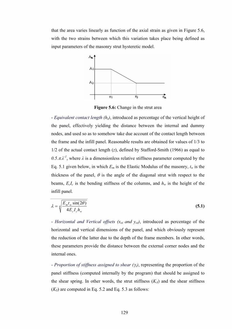
129

that the area varies linearly as function of the axial strain as given in Figure 5.6,

with the two strains between which this variation takes place being defined as

input parameters of the masonry strut hysteretic model.

Figure 5.6: Change in the strut area

- Equivalent contact length (hz), introduced as percentage of the vertical height of

the panel, effectively yielding the distance between the internal and dummy

nodes, and used so as to somehow take due account of the contact length between

the frame and the infill panel. Reasonable results are obtained for values of 1/3 to

1/2 of the actual contact length (z), defined by Stafford-Smith (1966) as equal to

0.5.π.λ-1, where λ is a dimensionless relative stiffness parameter computed by the

Eq. 5.1 given below, in which Em is the Elastic Modulus of the masonry, tw is the

thickness of the panel, θ is the angle of the diagonal strut with respect to the

beams, EcIc is the bending stiffness of the columns, and hw is the height of the

infill panel.

44

)2sin(

wcc

wm

hIEtE θ

λ = (5.1)

- Horizontal and Vertical offsets (xoi and yoi), introduced as percentage of the

horizontal and vertical dimensions of the panel, and which obviously represent

the reduction of the latter due to the depth of the frame members. In other words,

these parameters provide the distance between the external corner nodes and the

internal ones.

- Proportion of stiffness assigned to shear (γs), representing the proportion of the

panel stiffness (computed internally by the program) that should be assigned to

the shear spring. In other words, the strut stiffness (KA) and the shear stiffness

(KS) are computed in Eq. 5.2 and Eq. 5.3 as follows:

130

m

mmssA d

EAK

2)1( γ−= (5.2)

θγ 2cosm

mmsss d

EAK = (5.3)

- Specific weight (γ), representing the volumetric weight of the panel.

xoi, yoi, hz and tw are taken from the material test results for the shotcrete concrete

given in detail in Chapter 3, while A1 and A2 is predicted from the behaviour of the

wall during the test. γs is also predicted from the values taken from the interval given

in the manual depending on the test results.

5.5 Comparison of the Results of Analysis with Experimental Results

The analytical model prepared in SeismoStruct is shown in Figure 5.7 and 5.8.

Columns and beam are divided into 8 and 10 pieces, respectively as shown in Figure

5.9. The frame is idealized to have fixed type support. Three degrees of freedom, the

translational displacements, u, v and the rotation, θ, are considered at each node of

the frame and of the external and internal nodes of the wall.

For modelling the frame with the wall which is not connected to the columns, the xoi

and yoi are defined according to geometric properties of the wall. Although these

parameters are originally used to define the dimensions of the wall depending on the

depth of the frame elements, the obtained results show that it can also be used to

model these types of infill walls as well.

The analytical model was subjected to constant vertical point loads on the columns

and lateral displacement pattern which is acting at the centre of the loading beam as

shown in Figure 5.9.

Analytical studies start with modelling the bare frame first and then move onto the

shotcrete panel specimens. In the cross sections of the frame, unconfined and

confined concrete properties are taken into account by using existing models in the

program. A nonlinear response model existing in the program is assigned to the

reinforcements. Longitudinal reinforcement properties such as quantity, diameter and

coordinates and diameter and spacing of lateral reinforcement are introduced. The

shotcrete panel is modelled by diagonal braces corresponding to the infill wall model

131

in the program. Although there are several parameters existing in the program to

define the response of infill walls, the three parameters namely compressive strength,

tensile strength and shear resistance are the most effective ones.

The comparisons of the experimental and analytical results are presented only for

retrofitted non-damaged type frame specimens because the program is not capable of

modelling pre-damaged type frames.

Figure 5.7: Frame model used in SeismoStruct

Figure 5.8: Infilled frame models used in SeismoStruct

132

Figure 5.9: Definition of frame element names and the loadings in the mathematical model used in SeismoStruct

Damage states for structural members defined in Turkish Earthquake Code (TEC,

2007) are introduced to the program. Strain limits used to define damage states in

structural members are given in Table 5.6. At the end of the analysis, the program

produces reports about the damage states of the sections, which material inside this

section has reached the limit strain and at what stage of loading does the damage

occurred.

Table 5.6: Limit strain values to define damage states in structural members according to TEC 2007

Damage States in Structural Members Strain Limit Place of Deformation

Minimum Damage Limit (MNc) <- 0.0035 The outer-most fibre of the concrete of the

section Minimum Damage

Limit (MNs) > 0.01 Longitudinal reinforcement

Safety Limit (GVc) < -0.0085 The outer fibre of the concrete within the transversal reinforcement

Safety Limit (GVs) > 0.040 Longitudinal reinforcement

Collapse Limit (GCc) < -0.011 The outer fibre of the concrete within the transversal reinforcement

Collapse Limit (GCs) > 0.060 Longitudinal reinforcement

c = concrete, s = steel,

compression (-), tension (+) in strain limits

Constant Axial Forces on the Columns

Displacement Protocol

1

2 3

4

5

6

7

8 9 10 11 12 13 14 15 16 17 18 19

20

21

22

23

2425

26

0 500 1000 1500 2000 2500 3000

133

5.5.1 Specimen 1

The displacement history applied to Specimen 1 (bare frame) in the experimental

study is given in Figure 5.10. This loading protocol was applied to the analytical

model as well.

0 500 1000 1500 2000 2500 3000-50-40-30-20-10

01020304050

Top

Dis

plac

emen

t [m

m]

Step

Figure 5.10: The displacement pattern applied to Specimen 1

The comparison of the experimental and analytical results for Specimen 1 is given as

hysteretic loops in Figure 5.11 and as envelope curves in Figure 5.12. The envelope

curves are obtained by taking the average of load values corresponding to the three

cycles of the target displacements.

-50 -40 -30 -20 -10 0 10 20 30 40 50-200

-100

0

100

200

Bas

e Sh

ear

[kN

]

Displacement [mm]

Experimental Analytical

Figure 5.11: Comparison of the hysteretic curves of the experimental and analytical

results of Specimen 1

134

-50 -40 -30 -20 -10 0 10 20 30 40 50-200

-100

0

100

200B

ase

Shea

r [k

N]

Displacement [mm]


Figure 5.12: Comparison of the envelope curves of the experimental and analytical


As seen from Figure 5.11 analytical study overestimates strength values at the initial

displacement cycles. The maximum load occurred in the system is captured quiet

well in the analysis. But the descending branch slope of the analytical results is

steeper than the experimental results.

Table 5.7 summarizes the damage states observed in the analytical work. The table

summarizes the location of damage and which type of material is damaged. The

strain values are also given at the state of the damage. The bold lines in the table

match with the experimental result. The analytical results show almost the exact step

and position of damage like it has been observed during the experiment.

Figure 5.13 shows the damage states obtained at drift levels. For the pushing cycles,

“yield” has occurred first at the bottom and top end of the right column at 0.35% drift

levels. Unconfined concrete has reached “minimum damage limit” first at the bottom

and top end of the right and the left columns at 0.75% drift level. Reinforcement has

reached “minimum damage limit” first at the bottom end of the right column at

1.00% drift levels. Unconfined concrete has reached “safety and collapse limit” first

at the bottom end of the left column at 2.00% drift level. For the pulling cycles, at

0.35% drift level, yield occurred at the bottom and top end of the left column.

Unconfined concrete has reached “minimum damage limit” first at the bottom end of

the right column at 1.00% drift level. Reinforcement has reached “minimum damage

limit” at the bottom part and top end of the left column, and also at end of the beam

135

at 2.00% drift levels. At the same drift level unconfined concrete has reached “safety

and collapse limit” at the bottom end of the right column.

Table 5.7: Damage levels for Specimen 1

Target Displacement [mm] Performance Level

Element name

Place of damage Damage type Strain

At the end of 2nd cycle of +4.9 yield 1 Bottom end Steel 0.002404At the end of 3rd cycle of +4.9 yield 8 Top end Steel 0.002373At the end of 1st cycle of +5.6 yield 1 Top end Steel 0.002116At the end of 1st cycle of -5.6 yield 26 Bottom end Steel 0.002114At the end of 1st cycle of -5.6 yield 26 Top end Steel 0.002279At the end of 2nd cycle of -5.6 yield 18 Right end Steel 0.002161At the end of 3rd cycle of -5.6 yield 18 Left end Steel 0.002270At the end of 1st cycle of +7.0 yield 8 Bottom end Steel 0.002203At the end of 1st cycle of +10.5 MNc 26 Bottom end Unc Conc -0.003720At the end of 1st cycle of +10.5 MNc 1 Top end Unc Conc -0.003510At the end of 1st cycle of +10.5 MNc 8 Top end Unc Conc -0.003650At the end of 1st cycle of -10.5 yield 19 Top end Steel 0.002301At the end of 1st cycle of -10.5 yield 19 Bottom end Steel 0.002406At the end of 3rd cycle of +10.5 MNc 19 Top end Unc Conc -0.003630At the end of 1st cycle of +14 MNs 1 Bottom end Steel 0.010224At the end of 1st cycle of +14 MNc 26 Top end Unc Conc -0.003710At the end of 1st cycle of -14 MNc 1 Top end Unc Conc -0.003500At the end of 1st cycle of +28 MNs 1 Top end Steel 0.010800At the end of 1st cycle of +28 MNs 8 Top end Steel 0.010119At the end of 1st cycle of +28 MNs 26 Bottom end Steel 0.010309At the end of 1st cycle of +28 MNc 8 Top end Unc Conc -0.003550At the end of 1st cycle of +28 MNs 8 Top end Steel 0.010418At the end of 1st cycle of +28 MNc 19 Bottom end Unc Conc -0.003580At the end of 1st cycle of +28 GVc 26 Bottom end Unc Conc -0.008640At the end of 1st cycle of +28 MNs 26 Top end Steel 0.010137At the end of 1st cycle of +28 MNs 19 Top end Steel 0.010674At the end of 1st cycle of +28 GCc 26 Bottom end Unc Conc -0.011280At the end of 1st cycle of -28 GVc 1 Bottom end Unc Conc -0.008980At the end of 1st cycle of -28 GCc 1 Bottom end Unc Conc -0.012110At the end of 1st cycle of -28 MNs 19 Bottom end Steel 0.010281At the end of 2nd cycle of +28 MNc 7 Top end Unc Conc -0.003520At the end of 2nd cycle of -28 MNc 25 Bottom end Unc Conc -0.003530At the end of 2nd cycle of -28 MNs 18 Right end Steel 0.010040At the end of 3rd cycle of -28 MNs 18 Left end Steel 0.010046At the end of 1st cycle of -42 yield 25 Bottom end Steel 0.002105At the end of 2nd cycle of +42 MNc 2 Bottom end Unc Conc -0.003510At the end of 2nd cycle of +42 MNc 2 Top end Unc Conc -0.003510At the end of 3rd cycle of -42 MNc 25 Top end Unc Conc -0.003520

136

-150

-100

-50

0

50

100

150

-0.04 -0.03 -0.02 -0.01 0 0.01 0.02 0.03 0.04

Drift

Bas

e Sh

ear

[kN

]

yieldMNc

MNs

MNc yield

GVc, GCc

MNs,GVc, GCc

Figure 5.13: Damage states obtained at drift levels at certain drift levels at Specimen 1

Figure 5.14 shows the frame at the end of loading history. The “collapse limit” is

attained at the bottom ends of the columns.

Mn Gv Gc

Figure 5.14: Damages occurred at the end of the analysis of Specimen 1

5.5.2 Specimen 3

The displacement history applied to Specimen 3 (fully infilled frame) in the

experimental study is given in Figure 5.15. This loading protocol was used for the

analytical model as well.

137

0 500 1000 1500 2000 2500 3000 3500-20

-10

0

10

20

Top

Dis

plac

emen

t [m

m]

Step Figure 5.15: The displacement pattern applied to Specimen 3


hysteretic loops in Figure 5.16 and as envelope curves in Figure 5.17.

-20 -10 0 10 20-300

-200

-100

0

100

200

300

Bas

e Sh

ear

[kN

]

Displacement [mm]




138

-20 -10 0 10 20-300

-200

-100

0

100

200

300B

ase

Shea

r [k

N]

Displacement [mm]




As seen from Figure 5.16, analytical study predicts strength values at the initial

displacement cycles quiet well. The maximum load occurred in the system is

underestimated in the analysis. But the ultimate strength values are captured by

analytical results agrees well with the experimental results.

Table 5.8 summarizes the damage states observed in the analytical work. The table

summarizes the location of damage and which type of material is damaged with

strain value at the damage. The bold line in the table, match with the experimental

result. The analytical results show almost the exact step and position of damage like

it has been observed during the experiment.


“yield” has occurred first at the bottom and top end of the right column at 0.25% drift

levels. Unconfined concrete has reached “minimum damage limit” first at top ends of

the right and the left columns at 0.40% drift level. Reinforcement has reached

“minimum damage limit” first at the bottom end of the right column at 1.00% drift

levels. For the pulling cycles, at 0.25% drift level, “yield occurred” and unconfined

concrete has reached “minimum damage limit” at the top end of the left column.

Reinforcement has reached “minimum damage limit” at the bottom end of the left

column at 1.00% drift levels. At the same drift level confined concrete has reached

“safety limit” at the bottom end of the right column.

139


Target Displacement Performance Level

Element Name

Place of Damage

Damage type Strain

At the end of 2nd cycle of +3.5 yield 1 Bottom end Steel 0.002102At the end of 2nd cycle of +3.5 yield 8 Top end Steel 0.002101At the end of 3rd cycle of +3.5 yield 8 Bottom end Steel 0.002138At the end of 3rd cycle of -3.5 MNc 19 Top end Unc Conc -0.003531At the end of 3rd cycle of -3.5 yield 19 Top end Steel 0.002113At the end of 1st cycle of +4.9 yield 1 Top end Steel 0.002202At the end of 1st cycle of -4.9 yield 19 Bottom end Steel 0.002305At the end of 1st cycle of +5.6 MNc 20 Bottom end Unc Conc -0.003554At the end of 1st cycle of +5.6 MNc 8 Top end Unc Conc -0.003742At the end of 1st cycle of -5.6 yield 26 Bottom end Steel 0.002222At the end of 1st cycle of -5.6 yield 26 Top end Steel 0.002107At the end of 2nd cycle of -5.6 MNc 2 Top end Unc Conc -0.003524At the end of 3rd cycle of -5.6 MNc 2 Bottom end Unc Conc -0.003545At the end of 3rd cycle of -5.6 MNc 19 Bottom end Unc Conc -0.003503At the end of 1st cycle of +7.0 MNc 1 Bottom end Unc Conc -0.003639At the end of 1st cycle of +7.0 MNc 20 Top end Unc Conc -0.003733At the end of 1st cycle of -7.0 MNc 7 Bottom end Unc Conc -0.003511At the end of 1st cycle of +10.5 MNc 8 Bottom end Unc Conc -0.003511At the end of 1st cycle of +10.5 MNc 25 Top end Unc Conc -0.003514At the end of 1st cycle of +10.5 MNc 26 Bottom end Unc Conc -0.003697At the end of 1st cycle of -10.5 MNc 7 Top end Unc Conc -0.003530At the end of 1st cycle of -10.5 yield 20 Top end Steel 0.002963At the end of 2nd cycle of -10.5 MNc 25 Bottom end Unc Conc -0.003628At the end of 1st cycle of +14.0 MNc 26 Top end Unc Conc -0.003511At the end of 1st cycle of +14.0 MNc 1 Top end Unc Conc -0.003508At the end of 1st cycle of +14.0 MNs 1 Bottom end Steel 0.010083At the end of 1st cycle of -14.0 MNc 3 Bottom end Unc Conc -0.003571At the end of 1st cycle of -14.0 MNs 26 Bottom end Steel 0.010039At the end of 2nd cycle of +14.0 MNc 24 Bottom end Unc Conc -0.003523At the end of 3rd cycle of -14.0 GVc 1 Bottom end Conf Conc -0.008617

140

-300

-200

-100

0

100

200

300

-0.015 -0.010 -0.005 0.000 0.005 0.010 0.015

Drift

Bas

e Sh

ear

[kN

] yield

MNc

MNs

yield, MNc

MNs, GVc

Figure 5.18: Damage states obtained at drift levels at certain drift levels at

Specimen 3

Figure 5.19 shows the frame at the end of loading. The “safety limit” is reached at

the bottom end parts of the columns.

Mn Gv Gc

Figure 5.19: Damage occurred at the end of the analysis at Specimen 3

5.5.3 Specimen 5

The displacement history applied to Specimen 5 (partially infilled frame) in the

experimental study is given in Figure 5.20. This loading protocol was applied to the

analytical model as well.

141

0 500 1000 1500 2000 2500 3000 3500 4000 4500-50-40-30-20-10

01020304050

Top

Dis

plac

emen

t [m

m]

Step




-50 -40 -30 -20 -10 0 10 20 30 40 50-300

-200

-100

0

100

200

300

Bas

e Sh

ear

[kN

]

Displacement [mm]


Figure 5.21: Comparison of the hysteretic curves of the experimental and analytical results of Specimen 5

142

-50 -40 -30 -20 -10 0 10 20 30 40 50-300

-200

-100

0

100

200

300B

ase

Shea

r [k

N]

Displacement [mm]




As seen from Figure 5.21, analytical study predicts strength values at the initial

displacement cycles quiet well. The maximum load occurred in the system is

captured quiet good in the analysis as well. But the descending branch slope of the

analytical results is steeper than the experimental results.

Table 5.9 summarizes the damages states observed in the analytical work. The table

summarizes the location of damage and which type of material is damaged with

strain value at the damage. The bold lines in the table match with the experimental

result. The analytical results show almost the exact step and position of damage like

it has been observed during the experiment.


“yield” has occurred first at the bottom end of the right column at 0.25% drift level.

Unconfined concrete has reached “minimum damage limit” first at top end of the

right and the bottom end of the left column at 0.40% drift level. Reinforcement has

reached “minimum damage limit” first at the bottom and top end of the right column

at 1.00% drift levels. Confined concrete has reached “safety and collapse limit” at the

bottom ends of the right and left column at 2% drift level. Reinforcement has reached

“safety limit” at the bottom end of the left column at 3% drift level. For the pulling

cycles, at 0.3% drift level “yield” occurred at the end of the beam. Unconfined

concrete has reached “minimum damage limit” first at top ends of the right and the

left column at 0.50% drift level. Reinforcement has reached “minimum damage

143

limit” at the bottom end of the left column and at the end of the beam at 1.00% drift

level. At the same drift level confined concrete has reached “safety limit” at the

bottom end of the right column. Confined concrete has reached “collapse limit” at

the bottom end of the left column at 2.00% drift level. Reinforcement has reached

“safety limit” at the top end of the left column at 3.00% drift level.



Element Name

Place of Damage

Damage type Strain

At the end of 1st cycle of +3.5 yield 1 Bottom end Steel -0.002110At the end of 1st cycle of +4.2 yield 1 Top end Steel 0.002105At the end of 1st cycle of -4.2 yield 18 Top end Steel 0.002182At the end of 1st cycle of -4.2 yield 18 Bottom end Steel 0.002335At the end of 3rd cycle of +4.9 yield 8 Top end Steel 0.002256At the end of 3rd cycle of -4.9 yield 26 Bottom end Steel 0.002114At the end of 1st cycle of +5.6 yield 8 Bottom end Steel 0.002186At the end of 1st cycle of -5.6 yield 26 Top end Steel 0.002123At the end of 3rd cycle of +5.6 MNc 8 Top end Unc Conc -0.003720At the end of 3rd cycle of +5.6 MNc 25 Top end Unc Conc -0.003566At the end of 1st cycle of +7.0 MNc 19 Bottom end Unc Conc -0.003553At the end of 3rd cycle of -7.0 MNc 19 Top end Unc Conc -0.003561At the end of 3rd cycle of -7.0 MNc 7 Bottom end Unc Conc -0.003514At the end of 1st cycle of +10.5 MNc 25 Bottom end Unc Conc -0.003518At the end of 1st cycle of +10.5 MNc 26 Bottom end Unc Conc -0.003719At the end of 1st cycle of -10.5 MNc 1 Bottom end Unc Conc -0.003705At the end of 2nd cycle of -10.5 yield 19 Bottom end Steel 0.002180At the end of 3rd cycle of +10.5 MNc 8 Bottom end Unc Conc -0.003570At the end of 1st cycle of +14.0 MNc 20 Bottom end Unc Conc -0.003606At the end of 1st cycle of +14.0 MNs 8 Bottom end Steel 0.010086At the end of 1st cycle of +14.0 MNs 1 Bottom end Steel 0.010204At the end of 1st cycle of -14.0 yield 9 Bottom end Steel 0.002149At the end of 1st cycle of -14.0 yield 9 Top end Steel 0.002245At the end of 1st cycle of -14.0 yield 19 Bottom end Steel 0.002198At the end of 1st cycle of -14.0 MNs 26 Bottom end Steel 0.010101At the end of 2nd cycle of -14.0 MNs 18 Bottom end Steel 0.010428At the end of 3rd cycle of +14.0 MNc 7 Top end Unc Conc -0.003643At the end of 3rd cycle of -14.0 GVc 1 Bottom end Conf Conc -0.008574At the end of 3rd cycle of -14.0 MNs 18 Top end Steel 0.010508At the end of 1st cycle of +28.0 MNc 20 Top end Unc Conc -0.003528At the end of 1st cycle of +28.0 MNs 8 Top end Steel 0.010191At the end of 1st cycle of +28.0 MNc 26 Top end Unc Conc -0.003513At the end of 1st cycle of +28.0 MNs 1 Top end Steel 0.010049At the end of 1st cycle of +28.0 GVc 26 Bottom end Conf Conc -0.008906At the end of 1st cycle of +28.0 GCc 26 Bottom end Conf Conc -0.011526At the end of 1st cycle of +28.0 yield 20 Top end Steel 0.002292At the end of 1st cycle of +28.0 MNc 1 Top end Unc Conc -0.003579At the end of 1st cycle of +28.0 MNs 20 Top end Steel 0.010176At the end of 1st cycle of -28.0 GCc 1 Bottom end Conf Conc -0.011495At the end of 1st cycle of -28.0 MNs 26 Top end Steel 0.010212At the end of 1st cycle of -28.0 MNc 9 Bottom end Unc Conc -0.003527

144

Table 5.9: Damage levels for Specimen 5 (contd.)


Element Name

Place of Damage

Damage type Strain

At the end of 1st cycle of -28.0 MNs 19 Top end Steel 0.010350 At the end of 1st cycle of -28.0 MNs 19 Bottom end Steel 0.010220 At the end of 2nd cycle of +28.0 MNc 2 Bottom end Unc Conc -0.003567 At the end of 2nd cycle of +28.0 MNc 2 Top end Unc Conc -0.003542 At the end of 2nd cycle of +28.0 yield 2 Bottom end Steel 0.002189 At the end of 2nd cycle of -28.0 MNc 9 Top end Unc Conc -0.003511 At the end of 2nd cycle of -28.0 yield 20 Bottom end Steel 0.002104 At the end of 3rd cycle of +28.0 yield 7 Top end Steel 0.002105 At the end of 3rd cycle of +28.0 GVc 2 Bottom end Conf Conc -0.008507 At the end of 3rd cycle of -28.0 yield 25 Bottom end Steel 0.002154 At the end of 3rd cycle of -28.0 MNs 9 Bottom end Steel 0.010117 At the end of 3rd cycle of -28.0 MNs 9 Top end Steel 0.010173 At the end of 1st cycle of +42.0 yield 7 Bottom end Steel 0.002100 At the end of 1st cycle of +42.0 MNs 7 Bottom end Steel 0.010385 At the end of 1st cycle of -42.0 GVs 8 Top end Steel 0.040009 At the end of 1st cycle of -42.0 GVc 26 Top end Conf Conc -0.008519 At the end of 2nd cycle of -42.0 GVs 19 Bottom end Steel 0.040078 At the end of 2nd cycle of -42.0 GCc 26 Top end Conf Conc -0.011038 At the end of 3rd cycle of +42.0 yield 2 Top end Steel 0.002102 At the end of 3rd cycle of +42.0 GCc 2 Bottom end Conf Conc -0.011014 At the end of 3rd cycle of +42.0 GVc 2 Top end Conf Conc -0.008707 At the end of 3rd cycle of +42.0 GCc 2 Top end Conf Conc -0.011108 At the end of 3rd cycle of +42.0 MNs 2 Top end Steel 0.010352 At the end of 3rd cycle of +42.0 GVs 26 Bottom end Steel 0.040103 At the end of 3rd cycle of -42.0 yield 25 Top end Steel 0.002336 At the end of 3rd cycle of -42.0 GVc 25 Bottom end Conf Conc -0.008544 At the end of 3rd cycle of -42.0 MNs 25 Bottom end Steel 0.010253 At the end of 3rd cycle of -42.0 GVs 1 Bottom end Steel 0.040083 At the end of 3rd cycle of -42.0 MNs 25 Top end Steel 0.010413 At the end of 3rd cycle of -42.0 GVc 25 Top end Conf Conc -0.008577

-250-200

-150-100

-500

50100150

200250

-0.04 -0.03 -0.02 -0.01 0.00 0.01 0.02 0.03 0.04

Drift

Bas

e Sh

ear

[kN

]

yieldMNc

MNc MNs

yield GVc,GCc

MNs, GVcGCc

GVs

GVs


Specimen 5

145

Figure 5.24 shows the frame at the end of loading history the “collapse limit” and the

“safety limit” are reached at the bottom ends of the columns and at the top ends of

the columns, respectively.

Mn Gv Gc


5.5.4 Specimen 6

The displacement history applied to Specimen 6 (fully infilled frame with pre-reverse

deflection on the beam) in the experimental study is given in Figure 5.25. This

loading protocol was applied to the analytical model as well.

0 500 1000 1500 2000 2500 3000 3500-30

-20

-10

0

10

20

30

Top

Dis

plac

emen

t [m

m]

Step




146

-50 -40 -30 -20 -10 0 10 20 30 40 50-400

-300

-200

-100

0

100

200

300

400B

ase

Shea

r [k

N]

Displacement [mm]




-50 -40 -30 -20 -10 0 10 20 30 40 50-400

-300

-200

-100

0

100

200

300

400

Bas

e Sh

ear

[kN

]

Displacement [mm]




As seen from Figure 5.26, analytical study captured strength values at the initial

displacement cycles, maximum load occurred in the system and the descending

branch slope of the analytical results quiet well.

Table 5.10 summarizes the damages states observed in the analytical study. It also

gives the location of damage and which type of material is damaged with strain value

at the damage. The bold lines in the table match with the experimental result. The

δ

δ

147

analytical results show almost the exact step and location of damage like it has been

observed during the experiment.



Element name

Place of damage

Damage type Strain

At the end of 2nd cycle of +1.4 yield 19 Bottom end Steel 0.002146At the end of 3rd cycle of -1.4 yield 8 Bottom end Steel 0.002124At the end of 3rd cycle of +2.8 MNc 19 Bottom end Unc Conc -0.003520At the end of 2nd cycle of +3.5 yield 26 Bottom end Steel 0.002137At the end of 2nd cycle of -3.5 MNc 1 Bottom end Unc Conc -0.003550At the end of 3rd cycle of -3.5 yield 1 Bottom end Steel 0.002123At the end of 1st cycle of +4.2 MNs 19 Top end Steel 0.010015At the end of 1st cycle of +4.2 yield 26 Top end Steel 0.002193At the end of 1st cycle of -4.2 yield 9 Left end Steel 0.002111At the end of 1st cycle of -4.2 yield 9 Right end Steel 0.002174At the end of 2nd cycle of +4.2 MNc 26 Bottom end Unc Conc -0.003530At the end of 3rd cycle of -4.2 MNs 14 Left end Steel 0.010047At the end of 1st cycle of -5.6 MNs 14 Right end Steel 0.010047At the end of 2nd cycle of +5.6 MNc 26 Top end Unc Conc -0.003600At the end of 1st cycle of +7.0 yield 1 Top end Steel 0.002264At the end of 3rd cycle of -7.0 MNs 9 Left end Steel 0.010232At the end of 3rd cycle of -7.0 MNs 9 Right end Steel 0.010072At the end of 1st cycle of +10.5 MNc 1 Top end Unc Conc -0.003510At the end of 1st cycle of -10.5 yield 16 Left end Steel 0.002141At the end of 1st cycle of -10.5 MNc 2 Bottom end Unc Conc -0.003580At the end of 1st cycle of +14 GVc 26 Bottom end Conf Conc -0.008560At the end of 1st cycle of +14 MNc 8 Bottom end Unc Conc -0.003560At the end of 1st cycle of -14 yield 16 Right end Steel 0.002286At the end of 2nd cycle of +14 MNc 20 Top end Unc Conc -0.003670At the end of 2nd cycle of +14 yield 20 Top end Steel 0.002236At the end of 3rd cycle of +14 GCc 26 Bottom end Conf Conc -0.011080At the end of 3rd cycle of -14 MNc 9 Left end Unc Conc -0.003530At the end of 3rd cycle of -14 MNc 9 Right end Unc Conc -0.003530At the end of 1st cycle of +28 MNs 26 Bottom end Steel 0.010484At the end of 1st cycle of +28 MNs 1 Bottom end Steel 0.010091At the end of 1st cycle of +28 MNc 7 Top end Unc Conc -0.003510At the end of 1st cycle of +28 MNs 1 Top end Steel 0.010088At the end of 1st cycle of +28 MNs 8 Bottom end Steel 0.010336At the end of 1st cycle of +28 MNs 8 Top end Steel 0.010287At the end of 1st cycle of +28 GVc 1 Bottom end Conf Conc -0.008690At the end of 1st cycle of +28 MNc 7 Bottom end Unc Conc -0.003540At the end of 1st cycle of -28 MNc 25 Bottom end Unc Conc -0.003520At the end of 1st cycle of -28 yield 25 Bottom end Steel 0.002188At the end of 1st cycle of -28 GCc 1 Bottom end Conf Conc -0.011070At the end of 1st cycle of -28 GVc 25 Bottom end Conf Conc -0.008950At the end of 1st cycle of -28 GCc 25 Bottom end Conf Conc -0.011850At the end of 1st cycle of -28 MNs 25 Bottom end Steel 0.010252At the end of 2nd cycle of +28 yield 7 Top end Steel 0.002283At the end of 2nd cycle of +28 MNs 7 Top end Steel 0.010898At the end of 3rd cycle of +28 GVc 1 Top end Conf Conc -0.008910At the end of 3rd cycle of -28 MNc 25 Top end Unc Conc -0.003510

148


“yield” has occurred first at the top end of the left column at 0.10% drift levels.

Unconfined concrete has reached “minimum damage limit” first at top end of the left

columns at 0.20% drift level. Reinforcement has reached “minimum damage limit”

first at the bottom end of the left column at 0.30% drift levels. Confined concrete has

reached “safety and collapse limit” at the bottom end of the left column at 1.00%

drift level. For the pulling cycles, at 0.10% drift level “yield” occurred. Unconfined

concrete has reached “minimum damage limit” at the bottom end of the right column

at 0.25% drift level. Reinforcement has reached “minimum damage limit” at the

middle of the beam at 0.30% drift level. Confined concrete has reached “safety and

collapse limit” at the bottom end of the left column and “collapse limit” at the bottom

end of the right column at 2% drift level.

-400

-300

-200

-100

0

100

200

300

400

-0.03 -0.02 -0.01 0.00 0.01 0.02 0.03

Drift

Bas

e Sh

ear

[kN

]

MNc

yield

MNs

MNs

yield

MNc

GCc, GVc

GVc,GCc


Specimen 6

Figure 5.29 shows the frame at the end of loading history. The “collapse limit” is

reached at the bottom ends of the columns.

149

Mn Gv Gc


5.5.5 Specimen 7

The displacement history applied to Specimen 7 (partially infilled frame with pre-

reverse deflection on the beam) in the experimental study is given in Figure 5.30.

This loading protocol was applied to the analytical model as well.

0 500 1000 1500 2000 2500 3000 3500 4000 4500-50-40-30-20-10

01020304050

Top

Dis

plac

emen

t [m

m]

Step




150

-50 -40 -30 -20 -10 0 10 20 30 40 50-300

-200

-100

0

100

200

300B

ase

Shea

r [k

N]

Displacement [mm]




-50 -40 -30 -20 -10 0 10 20 30 40 50-300

-200

-100

0

100

200

300

Bas

e Sh

ear

[kN

]

Displacement [mm]




As seen from Figure 5.31, analytical study captured strength values at the initial

displacement cycles, maximum load occurred in the system and the descending

branch slope of the analytical results quiet well.

Table 5.16 summarizes the damages states observed in the analytical work. It also

gives the location of damage and which type of material is damaged with strain value

of the damage. The bold lines in the table match with the experimental result. The

analytical results show almost the exact step and position of damage like it has been

observed during the experiment.

δ

δ

151



Element name


At the end of 1st cycle of +2.8 yield 19 Bottom end Steel 0.002136At the end of 1st cycle of -2.8 yield 8 Bottom end Steel 0.002114At the end of 2nd cycle of +3.5 yield 26 Bottom end Steel 0.002113At the end of 3rd cycle of -3.5 MNc 1 Bottom end Unc Conc -0.003570At the end of 3rd cycle of -3.5 yield 1 Bottom end Steel 0.002359At the end of 3rd cycle of -3.5 MNc 8 Bottom end Unc Conc -0.003540At the end of 1st cycle of +4.2 MNc 26 Bottom end Unc Conc -0.003540At the end of 1st cycle of +4.2 yield 26 Top end Steel 0.002115At the end of 1st cycle of -4.9 MNc 1 Top end Unc Conc -0.003600At the end of 2nd cycle of +4.9 MNc 19 Bottom end Unc Conc -0.003510At the end of 1st cycle of -5.6 yield 16 Right end Steel 0.002154At the end of 1st cycle of -5.6 yield 16 Left end Steel 0.002165At the end of 1st cycle of +7.0 MNs 19 Top end Steel 0.010120At the end of 1st cycle of +7.0 MNc 26 Top end Unc Conc -0.003520At the end of 2nd cycle of +7.0 MNc 2 Bottom end Unc Conc -0.003540At the end of 2nd cycle of -7.0 MNc 2 Top end Unc Conc -0.003550At the end of 3rd cycle of +7.0 yield 1 Top end Steel 0.002135At the end of 3rd cycle of +7.0 yield 11 Left end Steel 0.002108At the end of 3rd cycle of +7.0 yield 11 Right end Steel 0.002104At the end of 3rd cycle of -7.0 MNs 16 Left end Steel 0.010023At the end of 3rd cycle of -7.0 MNs 16 Right end Steel 0.010015At the end of 1st cycle of -10.5 yield 17 Left end Steel 0.002222At the end of 1st cycle of -10.5 yield 17 Right end Steel 0.002111At the end of 1st cycle of -10.5 MNs 8 Top end Steel 0.010023At the end of 3rd cycle of -10.5 GVc 26 Bottom end Conf Conc -0.008690At the end of 1st cycle of -14.0 yield 18 Right end Steel 0.002148At the end of 1st cycle of -14.0 yield 18 Left end Steel 0.002188At the end of 1st cycle of -14.0 GVc 1 Bottom end Conf Conc -0.008800At the end of 1st cycle of -14.0 MNc 25 Bottom end Unc Conc -0.003530At the end of 1st cycle of -14.0 yield 25 Bottom end Steel 0.002133At the end of 2nd cycle of +14.0 GCc 26 Bottom end Conf Conc -0.011170At the end of 3rd cycle of +14.0 MNs 26 Bottom end Steel 0.010239At the end of 3rd cycle of -14.0 GCc 1 Bottom end Conf Conc -0.011030At the end of 3rd cycle of -14.0 yield 25 Bottom end Steel 0.002105At the end of 1st cycle of +28.0 yield 10 Right end Steel 0.002127At the end of 1st cycle of +28.0 yield 10 Left end Steel 0.002135At the end of 1st cycle of +28.0 MNc 20 Top end Unc Conc -0.003530At the end of 1st cycle of +28.0 yield 2 Bottom end Steel 0.002114At the end of 1st cycle of +28.0 MNs 1 Top end Steel 0.010109At the end of 1st cycle of +28.0 MNs 1 Bottom end Steel 0.010389At the end of 1st cycle of +28.0 yield 7 Top end Steel 0.002125At the end of 1st cycle of +28.0 MNc 7 Top end Unc Conc -0.003540At the end of 1st cycle of -28.0 MNc 25 Top end Unc Conc -0.003520At the end of 1st cycle of -28.0 MNs 26 Top end Steel 0.010168At the end of 2nd cycle of -28.0 MNc 3 Bottom end Unc Conc -0.003520At the end of 2nd cycle of -28.0 MNs 17 Right end Steel 0.010034At the end of 2nd cycle of -28.0 MNs 17 Left end Steel 0.010000At the end of 3rd cycle of +28.0 yield 2 Top end Steel 0.002135At the end of 3rd cycle of +28.0 MNs 7 Top end Steel 0.010071At the end of 1st cycle of +42.0 yield 7 Bottom end Steel 0.002155At the end of 1st cycle of -42.0 GVs 8 Top end Steel 0.040107

152

Table 5.11: Damage levels for Specimen 7 (contd.)


Element name


At the end of 1st cycle of -42.0 GVc 26 Top end Conf Conc -0.008570 At the end of 2nd cycle of +42.0 GVs 26 Bottom end Steel 0.040135 At the end of 2nd cycle of -42.0 MNs 18 Right end Steel 0.010168


“yield” has occurred first at the top end of the left column at 0.20% drift levels.

Unconfined concrete has reached “minimum damage limit” first at bottom end of the

left columns at 0.35% drift level. Reinforcement has reached “minimum damage

limit” first at the top end of the left column at 0.50% drift levels. Confined concrete

has reached “collapse limit” at the bottom end of the left column at 1.00% drift level.

Reinforcement has reached “safety limit” at the top end of the right column at 3.00%

drift level. For the pulling cycles, at 0.25% drift level “yield” occurred. Unconfined

concrete has reached “minimum damage limit” at the bottom end of the right column

at 0.30% drift level. Reinforcement has reached “minimum damage limit” at the end

of the beam at 0.50% drift level. Confined concrete has reached “safety limit” at the

bottom end of the left column at 0.75% drift level. Confined concrete has reached

“collapse limit” at the bottom end of the right column at 1.00% drift level.

Reinforcement has reached “safety limit” at the top end of the right column at 3.00%

drift level.

-250-200-150

-100-50

050

100

150200250

-0.04 -0.03 -0.02 -0.01 0.00 0.01 0.02 0.03 0.04

Drift

Bas

e Sh

ear

[kN

]

yieldMNc

yield

MNs

MNc

GVs

GVs

GCc

GCc

GVc

MNs


Specimen 7

153

Figure 5.34 shows the frame at the end of loading history. The “collapse limit” and

the “safety limit” are reached at the bottom ends of the columns and the upper end of

the column where the lateral load is applied.

Mn Gv Gc


155

6. PARAMETRIC STUDIES

In this chapter, the model produced for analysing the specimens in experimental

study is used to understand the effect of the change in panel thickness, the effect of

the concrete compressive strength of the panel and the gap between the panel and the

frame on the overall behaviour of the system.

6.1 The Effect of Panel Thickness

The panel thickness is changed proportional to the column width as shown in Table

6.1, the bold line corresponds to the thickness of the specimen in the experimental

study. By using the models produced for Specimen 3 (fully infilled frame) and

Specimen 5 (partially infilled frame), the effect of change in the panel thickness is

studied.

Table 6.1: The change in the thickness of the panel

Case Column width [cm]

Thickness of the panel [cm]

Thickness proportion

1 20 5 0.25 2 20 10 0.50 3 20 15 0.75 4 20 20 1.00

Figure 6.1 shows the change in the lateral load carrying capacity of Specimen 3

according to the thickness change in the panel. The envelope curves of base shear

versus displacement relations are only given for the pushing cycles in Figure 6.2. The

points on the envelope curves are calculated as the average of the three cycles at each

target displacement levels.

156

Infill panel thickness = 5 cm

-800

-600-400

-200

0

200400

600

800

-20 -15 -10 -5 0 5 10 15 20

Displacement [mm]

Bas

e Sh

ear

[kN

] Infill panel thickness = 10 cm

-800-600

-400-200

0200

400600

800

-20 -15 -10 -5 0 5 10 15 20Displacement [mm]

Bas

e Sh

ear

[kN

]


-800

-600

-400

-2000

200

400

600

800

-20 -15 -10 -5 0 5 10 15 20Displacement [mm]

Bas

e Sh

ear

[kN

]


-800-600-400-200

0200400600800

-20 -15 -10 -5 0 5 10 15 20

Displacement [mm]

Bas

e Sh

ear

[kN

]

Figure 6.1: Base shear-top displacement curves for the infill panel thickness changes in Specimen 3

0 7 14 210

200

400

600

8000.000 0.005 0.010 0.015

Bas

e Sh

ear

[kN

]

Displacement [mm]

t = 5 cm t = 10 cm t = 15 cm t = 20 cm Bare Frame

Drift

Figure 6.2: Envelope curves for the thickness changes in Specimen 3

The lateral load carrying capacity of the frame increases as the thickness of the

shotcrete panel increases. This behaviour is valid until the thickness is 15 cm. The

Experiment

157

frames having 15 cm and 20 cm (which is the width of the column) thick panels

seem to have almost the same lateral load resistance.

The lateral load carrying capacity of the frames;

• When t=10 cm, it is 4.8 times more at 7 mm (0.5% story drift), it is 3.4 times

more at 14 mm (1% story drift),




more at 14 mm (1% story drift)

compared with the bare frame’s.

Initial stiffness changes depending on the thickness change is given in Figure 6.3.

0

50

100

150

200

250

300

350

Initi

al S

tiffn

ess [

kN/m

m]

Bare Framet = 5 cmt = 10 cmt = 15 cmt = 20 cm

Figure 6.3: Initial stiffness of Specimen 3 for the change in panel thickness

Energy dissipation capacities depending on the thickness change in panel are given

in Figure 6.4.

Experiment

158

0.000 0.005 0.0100

20000

40000

60000C

umul

ativ

e E

nerg

y D

issi

patio

n [k

Nm

m]

Story Drift

t=5 cm t=10 cm t=15 cm t=20 cm Bare Frame

Figure 6.4: The comparison of cumulative energy dissipation capacities of Specimen 3 for the change in panel thickness

The dissipated energy of the specimens;





• When t=20 cm, it is 10.4 times more at 7 mm (0.5% story drift), it is 5.5

times more at 14 mm (1% story drift),


As can be seen in Figure 6.1, the system behaviour of the frames with 15 and 20 cm

thick panels are almost the same. It is predicted that this behaviour is due to the high

difference between the concrete compressive strengths of the frame and the shotcrete

panel. For investigating the correctness of this prediction, Specimen 3 is studied

analytically for the case where the concrete compressive strengths of both frame and

panel are identical. The concrete compressive strengths are taken as 25 MPa and the

hysteretic and envelope curves of base shear versus top displacement obtained for

this case are shown in Figure 6.5 and 6.6, respectively. As can be seen in these

figures, the general response obtained is different for 15 and 20 cm thick panel cases

which prove the prediction.

Experiment

159


-1000-800-600-400-200

0200400600800

1000

-20 -15 -10 -5 0 5 10 15 20Displacement [mm]

Bas

e Sh

ear

[kN

]


-1000-800-600-400-200

0200400600800

1000

-20 -15 -10 -5 0 5 10 15 20Displacement [mm]

Bas

e Sh

ear

[kN

]


0 7 14 210

200

400

600

800

10000.000 0.005 0.010 0.015

Bas

e Sh

ear

[kN

]

Displacement [mm]

Bare Frame t = 15 cm t = 20 cm

Drift



according to the thickness change in the panel. The envelope curves are given in

Figure 6.8 for the pushing cycles.

160


-600

-400

-200

0

200

400

600

-50 -40 -30 -20 -10 0 10 20 30 40 50Displacement [mm]

Bas

e Sh

ear

[kN

] Infill panel thickness = 10 cm

-600

-400

-200

0

200

400

600

-50 -40 -30 -20 -10 0 10 20 30 40 50Displacement [mm]

Bas

e Sh

ear

[kN

]


-600

-400

-200

0

200

400

600

-50 -40 -30 -20 -10 0 10 20 30 40 50Displacement [mm]

Bas

e Sh

ear

[kN

]


-600

-400

-200

0

200

400

600

-50 -40 -30 -20 -10 0 10 20 30 40 50Displacement [mm]

Bas

e Sh

ear

[kN

]


0 14 28 42 560

200

400

6000.00 0.01 0.02 0.03 0.04

Bas

e Sh

ear

[kN

]

Displacement [mm]

t = 5 cm t = 10 cm t = 15 cm t = 20 cm Bare Frame

Drift


The lateral load carrying capacity increased by 1.6 times more for 10 cm-thick panel,

2.2 times more for 15 cm-thick panel and 2.8 times more for 20 cm-thick panel at 14

mm (0.01 story drift); 1.8 times more for 10 cm-thick panel, 2.5 times for 15 cm-

Experiment

161

thick panel and 3.2 times more for 20 cm-thick panel at 28 mm (0.02 story drift); 2.0

times for 10 cm-thick panel and 2.8 times for 15 cm-thick panel at 42 mm (0.03 story

drift) compared to the specimen in the experiment with 5 cm-thick panel..



more at 14 mm (1% story drift), it is 3.7 times more at 28 mm (2% story

drift), it is 4.8 times more at 42 mm (3% story drift),






drift),


Initial stiffness changes depending on the thickness change are given in Figure 6.9.

0

50

100

150

200

250

Initi

al S

tiffn

ess [

kN/m

m]

Bare Framet = 5 cmt = 10 cmt = 15 cmt = 20 cm

Figure 6.9: Initial stiffness of Specimen 5 for the change in panel thickness

The initial lateral stiffness of the frames;

• increased by 3.9 times for t=10 cm,




Experiment

162

Energy dissipation capacities depending on the thickness change in panel are given

in Figure 6.10.

0.00 0.01 0.02 0.03 0.040

20000

40000

60000

80000

Cum

ulat

ive

Ene

rgy

Dis

sipa

tion

[kN

mm

]

Story Drift

t=5 cm t=10 cm t=15 cm t=20 cm Bare Frame


Specimen 5 for the change in panel thickness

The energy dissipation of the specimens with 10 cm-thick panel and 15 cm-thick

panel compared to the test specimen (5cm-thick panel) are 1.6 and 2.0 times more at

0.005 story drift, 1.5 and 1.9 times more at 0.01 story drift, 1.4 and 1.7 times more at

0.02 story drift, 1.4 and 1.5 times more at 0.03 story drift respectively as shown in

Figure 6.8. The 15 cm-thick and 20 cm-thick panels have almost the same energy

dissipation capacity. Since the analysis for 20 cm-thick panel did not converge until

the end of the load pattern; it seems that they have the same energy dissipation

capacity at 0.02 story drift. But 20 cm-thick panel has only done two cycles of 28

mm target displacement. So actually the 15 cm-thick and 20 cm-thick panels don’t

have the same energy dissipation at 0.01 story drift.

The energy dissipation of the specimens;







Experiment

163



drift),


6.2 The Effect of the Distance between the Panel and the Frame

The gap, a, is changed proportional to the distance between the inside face of the

columns, L, as shown in Figure 6.11. The calculated gap size according to the

proportional ratio, a/L, and panel widths are given in Table 6.2 to be used in the

models produced for Specimen 5. The bold line in the table shows the thickness of

the specimen used in the experimental study.

Figure 6.11: The gap, a, and the distance between the inside face of the columns, L, in the model used

Table 6.2: The change in the distance between the column and the panel

Case L, Frame width [cm]

a; Gap between panel and column [cm] a/L Panel width

1 170 1.7 0.01 166.6 2 170 8.5 0.05 153.0 3 170 17.0 0.10 136.0 4 170 20.0 0.12 130.0 5 170 25.5 0.15 119.0 6 170 34.0 0.20 102.0

aL

a

164


according to the distance change between the column and the panel. The envelope

curves are given in Figure 6.13 for the pushing cycles.

a/L = 0.01

-300

-200

-100

0

100

200

300

-50 -40 -30 -20 -10 0 10 20 30 40 50Displacement [mm]

Bas

e Sh

ear

[kN

]

a/L = 0.05

-300

-200

-100

0

100

200

300

-50 -40 -30 -20 -10 0 10 20 30 40 50Displacement [mm]

Bas

e Sh

ear

[kN

]

a/L = 0.10

-300

-200

-100

0

100

200

300

-50 -40 -30 -20 -10 0 10 20 30 40 50Displacement [mm]

Bas

e Sh

ear

[kN

]

Experiment

-300

-200

-100

0

100

200

300

-50 -40 -30 -20 -10 0 10 20 30 40 50Displacement [mm]

Bas

e Sh

ear

[kN

]

a/L = 0.15

-300

-200

-100

0

100

200

300

-50 -40 -30 -20 -10 0 10 20 30 40 50Displacement [mm]

Bas

e Sh

ear

[kN

]

a/L = 0.20

-300

-200

-100

0

100

200

300

-50 -40 -30 -20 -10 0 10 20 30 40 50Displacement [mm]

Bas

e Sh

ear

[kN

]

Figure 6.12: Base shear-top displacement curves for the gap size changes in Specimen 5

165

0 14 28 42 560

100

200

3000.00 0.01 0.02 0.03 0.04

a/L = 0.01 a/L = 0.05 a/L = 0.10 a = 20 cm a/L = 0.15 a/L = 0.20 Bare Frame

Bas

e Sh

ear

[kN

]

Displacement [mm]

Drift

Figure 6.13: Envelope curves for the gap size changes in Specimen 5

The analytical study shows that when a/L ratio changes from 1% to 15%, the lateral

load carrying capacity of the system is almost the same. While a/L ratio is 20% or

more, the panel does not have any effect on the lateral load carrying capacity and the

frame acts like a bare frame.

The lateral load carrying capacity of the system;

• When a/L=0.01, it is 2.6 times more at 7 mm (0.5% story drift), it is 2.4 times












Experiment

166

• When a/L=0.20, it is 0.96 times less at 7 mm (0.5% story drift), it is 0.94

times less at 14 mm (1% story drift), it is 0.92 times less at 28 mm (2% story




• increased by 2.9 times for a=1.7 cm,

• increased by 2.9 times for a=8.5 cm,

• increased by 2.8 times for a=17 cm,

• increased by 2.5 times for a=25.5 cm

• no increase for a=34 cm


Energy dissipation capacities depending on the distance change between the panel

and the frame are given in Figure 6.12.

When a/L ratio varies between 1% to 15%, the energy dissipation of the specimen is

almost the same at all story drift levels. When a/L is 20%, the energy dissipation

capacity is 33%, 33%, 43% times less than the energy dissipation capacity of the test

specimen at 0.01, 0.02 and 0.03 story drift levels, respectively as shown in Figure

6.14.

0.00 0.01 0.02 0.03 0.040

20000

40000

60000

Cum

ulat

ive

Ene

rgy

Dis

sipa

tion

[kN

mm

]

Story Drift

a/L = 0.01 a/L = 0.05 a/L = 0.10 a = 20 cm a/L = 0.15 a/L = 0.20 Bare Frame


Specimen 5 for the gap size changes

Experiment

167














• When a/L=0.20, it is 0.98 times less at 7 mm (0.5% story drift), it is 1.0 times

less at 14 mm (1% story drift), it is 1.0 times less at 28 mm (2% story drift), it

is 0.92 times less at 42 mm (3% story drift),


6.3 Panel Concrete Compressive Strengths

To investigate how the panel concrete compressive strength effects the general

response of the system, an analytical study was carried on Specimen 3. The concrete

compressive strength of the panel was 22 MPa for the experiment. In the analytical

work, it is taken as 30 MPa and 40 MPa and the results are compared as hysteretic

loops, envelope curves and initial stiffness.


according to the concrete compressive strengths change in the panel. The envelope

curves are given in Figure 6.16 for the pushing cycles.

168

σ= 22 MPa

-500-400-300-200-100

0100200300400500

-20 -15 -10 -5 0 5 10 15 20Displacement [mm]

Bas

e Sh

ear

[kN

]

σ= 30 MPa

-500-400-300-200-100

0100200300400500

-20 -15 -10 -5 0 5 10 15 20Displacement [mm]

Bas

e Sh

ear

[kN

]

σ= 40 MPa

-500-400-300-200-100

0100200300400500

-20 -15 -10 -5 0 5 10 15 20Displacement [mm]

Bas

e Sh

ear

[kN

]

Figure 6.15: Base shear-top displacement curves for the infill panel concrete

compressive changes in Specimen 3

0 7 14 210

100

200

300

400

5000.000 0.005 0.010 0.015

Bas

e Sh

ear

[kN

]

Displacement [mm]

σ = 22 Mpa σ = 30 Mpa σ = 40 Mpa Bare Frame

Drift

Figure 6.16: Envelope curves for the infill panel concrete compressive changes in

Specimen 3

Experiment

169


• When σ=30 MPa,, it is 4.3 times more at 7 mm (0.5% story drift), it is 2.5


• When σ=40 MPa,, it is 5.3 times more at 7 mm (0.5% story drift), it is 3.0



Initial stiffness changes depending on the infill panel concrete compressive changes

are given in Figure 6.17.

0

50

100

150

200

Initi

al S

tiffn

ess [

kN/m

m]

Bare Frames= 22MPas= 30MPas= 40MPa

Figure 6.17: Initial stiffness of Specimen 3 for the infill panel concrete compressive changes


• increased by 3.8 times for σ=30 MPa,

• increased by 4.6 times for σ=40 MPa,


Energy dissipation capacities depending on the concrete compressive changes in

panel are given in Figure 6.18.

Experiment

170

0.000 0.005 0.0100

10000

20000

30000

40000C

umul

ativ

e E

nerg

y D

issi

patio

n [k

Nm

m]

Story Drift

σ=22 MPa σ=30 MPa σ=40 MPa Bare Frame


Specimen 3 for the infill panel concrete compressive changes


• When σ=30 MPa, it is 3.5 times more at 7 mm (0.5% story drift), it is 2.6


• When σ=40 MPa, it is 4.4 times more at 7 mm (0.5% story drift), it is 3.1



6.4 Application of the Retrofitting Technique to a Representative Frame

In this section, the proposed retrofitting technique is applied on a 2D frame of a

building representing the typical RC frame type structures in Turkey, (Girgin 1986,

Yıldız 2008). The elevation of the frame can be seen in Figure 6.19. The frame has

six storeys with a total height of 21 m. Storey heights are identical and equal to 3.5 m

and span lengths are 5 m. The slabs have a thickness of 15 cm.

Two outer spans of the frame, namely AB and DE, are filled with 15 cm thick

shotcrete panels as can be seen in Figure 6.20 for retrofitting purpose. Since the

geometry of the representative frame is almost 3 times bigger than the tested

specimens, the panel thickness is chosen as 15 cm.

171

Steel quality is S420a and concrete quality for frame and shotcrete panel are C16 and

C20, respectively. The dimensions and longitudinal reinforcement data of columns

are presented in Figure 6.21 and Table 6.3. The dimensions and longitudinal

reinforcement data of beams are presented in Figure 6.22 and Table 6.4. All the

beams are 300 mm in width and 600 mm in depth. The concrete cover of beams and

columns are selected as 40 mm. The lateral reinforcement of columns and beams are

φ10/200.

Figure 6.19: The representative frame

Figure 6.20: Retrofitting of the frame by shotcreted walls

A B C D E

6th

5th

4th

1st

2nd

3rd

172

Figure 6.21: Cross section of the column

Table 6.3: The dimensions and reinforcement of the columns

300 mm

150 mm

600 mm

600 mm

Figure 6.22: Cross section of the typical beam

Table 6.4: The reinforcement of the beams

Analytical study is conducted by using SeismoStruct to evaluate the effect of the

retrofitting technique on the response of the frame. The response parameters defined

for shotcrete panel in Chapter 5 are adapted here. Since the shotcrete panel used in

Axes Story A B C

5 - 6 a/b=300/400 mm 4Φ18 + 4Φ16

a/b=300/400 mm 4Φ16 + 4Φ16

b/a=400/300 mm 4Φ16 + 4Φ14

3 - 4 300/400 mm 4Φ18 + 4Φ16

300/500 mm 4Φ20 + 4Φ20

500/300 mm 4Φ20 + 4Φ20

1 - 2 300/400 mm 4Φ18 + 4Φ16

300/600 mm 4Φ22 + 4Φ20

600/300 mm 4Φ20 + 4Φ20

A – B Beam B – C Beam Story Place of

reinforcement Left support Span Right support

Left support Span Right

support Top 2φ12+2φ18 2φ12 2φ12+2φ18 2φ12+2φ18 2φ12 2φ12+2φ14 6 - 5

Bottom 3φ16 3φ16 3φ16 3φ16 3φ16 3φ16 Top 2φ14+3φ20 2φ14 2φ14+3φ20 2φ14+3φ20 2φ14 2φ14+2φ20 4 – 3 Bottom 4φ16 4φ16 4φ16 4φ16 4φ16 4φ16 Top 3φ14+2φ22 3φ14 3φ14+3φ22 3φ14+3φ22 3φ14 3φ14+1φ22 2 – 1 Bottom 4φ16 4φ16 4φ16 4φ16 4φ16 4φ16

a

b

173

this demonstrative example is aimed to be fully connected to outer frames, the

parameters obtained for Specimen 3 is used.

Two types of analysis have been carried out; pushover and nonlinear dynamic time

history analysis (NDTHA). The frame is idealized to have fixed type support in the

analysis.

Bilinear steel model is used to model the reinforcement given in Figure 6.23a. This is

a uniaxial bilinear stress-strain model with kinematic strain hardening, whereby the

elastic range remains constant throughout the various loading stages, and the

kinematic hardening rule for the yield surface is assumed as a linear function of the

increment of plastic strain.

Uniaxial nonlinear constant confinement concrete model is used for confined

concrete seen in Figure 6.23b.

-0.20 -0.16 -0.12 -0.08 -0.04 0.04 0.08 0.12 0.16 0.200.00

-400

-600

-200

-200

-600 -400

0

εs

σs [Mpa]

-0.002 -0.004 -0.006 -0.008 -0.010

-8

-12

-16

4 0.002

σc [Mpa]

εc

a) Steel b) Concrete

Figure 6.23: Constitutive models used in analytical study

Sum of the dead loads and 30% of the live loads are taken into account in the

calculation of seismic weight. The mass values used in the analysis are given in

Table 6.5 for two cases.

Table 6.5: Concentrated mass values at each floor levels

Storey mass [kNsec2/m] Storey Bare frame Shotcreted frame

6 49.0 55.6 5 78.7 92.0 4 79.7 93.0 3 80.3 93.6 2 81.2 94.6 1 80.9 94.2

174

The building is assumed to be constructed on firm soil (Z2 type) at seismic zone 1

defined in TEC, 2007.

The first natural vibrational periods for the bare frame and the shotcreted frame are

T1= 0.992 sec and T1= 0.430 sec, respectively. First mode shapes of both cases can

be seen in Figure 6.24.

Figure 6.24: First mode shapes of bare and retrofitted frame

In Table 6.6, the lateral load ratios to be used in the push-over analysis are

calculated. They are obtained from the static moments of the storey seismic weights

to the ground. The obtained lateral load distribution is close to 1st vibration mode of

the frames. The base shear-top displacement relation determined by the analysis is

presented in Figure 6.25. The stiffness and the maximum strength of the retrofitted

frame are expectedly much larger. In the case of the bare frame and the retrofitted

frame, maximum strength is about 0.16W and 0.39W, respectively. The displacement

capacity of the retrofitted frame decreased by 2.8 times compared to the bare frame.

Table 6.6: Forces applied during pushover analysis

a) Bare frame Storey Wi (kN) Hi (m) Wi*Hi (Wi*Hi)/∑(Wi*Hi)

6 480.87 21.0 10098.27 0.197 5 772.25 17.5 13514.38 0.264 4 782.01 14.0 10948.14 0.214 3 787.73 10.5 8271.16 0.162 2 796.60 7.0 5576.20 0.109 1 793.38 3.5 2776.83 0.054 ∑ 4412.84 5217.63 1.000

175

Table 6.6: Forces applied during pushover analysis (contd.)

b) Retrofitted frame Storey W (kN) Hi (m) Wi*Hi (Wi*Hi)/∑(Wi*Hi)

6 546.50 21.0 11476.48 0.193 5 903.50 17.5 15811.25 0.266 4 913.26 14.0 12785.65 0.215 3 918.98 10.5 9649.25 0.162 2 927.85 7.0 6494.96 0.109 1 924.63 3.5 3236.20 0.054 ∑ 5134.72 6060.53 1.000

0.0000 0.0525 0.1050 0.1575 0.2100 0.26250

980

1960

29400.0000 0.0025 0.0050 0.0075 0.0100 0.0125

0.0

0.2

0.4

0.6

Bas

e Sh

ear

[kN

]

Displacement [m]

Bare Frame Retrofitted Frame

Bas

e Sh

ear/

Tot

al W

eigh

t [kN

/kN

]

Displacement/Total Height [m/m]

Figure 6.25: Base shear-top displacement and base shear/total weight-top displacement/total height diagram

Nonlinear dynamic time history analysis (NDTHA) is also performed. Three

earthquake records were taken from PEER (2007) data bank to generate artificial

accelerograms. The detailed information about the earthquakes is given in Table 6.7.

The original earthquake acceleration records are drawn in Figure 6.26, 6.27 and 6.28.

Table 6.7: Earthquake records

Earthquake Date Station / Direction M PGA (g)

Erzincan 13.03.1992 Erzincan / EW 6.9 0.496 İzmit 17.08.1999 İzmit / 090 7.4 0.220 Düzce 12.11.1999 Bolu / 090 7.1 0.822

176

-8-6-4-202468

0 10 20 30 40 50 60Time [sec]

Acc

eler

atio

n [m

/sec2

]

Erzincan 1992

Figure 6.26: The acceleration record of Erzincan Earthquake

-8-6-4-202468

0 10 20 30 40 50 60Time [sec]

Acc

eler

atio

n [m

/sec2

]

Izmit 1999

Figure 6.27: The acceleration record of İzmit Earthquake

-8-6-4-202468

0 10 20 30 40 50 60Time [sec]

Acc

eler

atio

n [m

/sec2

]

Duzce 1999

Figure 6.28: The acceleration record of Düzce Earthquake

The original acceleration records of the three earthquakes given above are modified

respect to the acceleration spectra defined for Z2 type soil given in TEC, 2007. Two

versions of the earthquakes are produced named as “service” and “design”

earthquakes, (Yıldız, 2008).

The modified earthquake records obtained are given in Figure 6.29 as “service” and

in Figure 6.30 as “design” earthquakes.

177

-8-4048

0 10 20 30 40 50 60

Time [sec]a

Erzincan

Acc

eler

atio

n [m

/sec

2]

-8-4048

0 10 20 30 40 50 60

Time [sec]

A

Izmit

Acc

eler

atio

n [m

/sec

2]

-8-4048

0 10 20 30 40 50 60

Time [sec]

Ac

Duzce

Acc

eler

atio

n [m

/sec

2]

Figure 6.29: “Service” type acceleration records

-8-4048

0 10 20 30 40 50 60

Time [sec]

A

Erzincan

Acc

eler

atio

n [m

/sec

2]

-8-4048

0 10 20 30 40 50 60

Time [sec]

A

Izmit

Acc

eler

atio

n [m

/sec

2]

-8-4048

0 10 20 30 40 50 60

Time [sec]

A

Duzce

Acc

eler

atio

n [m

/sec

2]

Figure 6.30: “Design” type acceleration records

178

The mean spectrum of the modified design earthquakes is drawn with the design

spectrum for Z2 type soil in Figure 6.31.

0

2

4

6

8

10

12

0 0.5 1 1.5 2 2.5 3 3.5 4Time [sec]

Sae

[m/se

c2]

Z2 Design SpectraMean Spectra

Figure 6.31: Design spectrum defined in TEC, 2007

In NDTHA, the direct integration of the equations of motion is accomplished using

the numerically dissipative α-integration algorithm Hilber et al. (1977) with

automatic time-step adjustment for optimum accuracy and efficiency.

For each increment, several iterations are carried out until convergence is achieved.

If convergence is not reached within the specified maximum number of iterations,

the load increment (or time-step) is reduced and the analysis is restarted from the last

point of equilibrium (end of previous increment or time-step). This step reduction,

however, is not constant but rather adapted to the level of non-convergence verified.

At the end of a solution step or increment; a convergence ratio indicator, defined as

the maximum of ratios between the achieved and the required displacement/force

convergence factors is computed. Then, depending on how far away the analysis was

from reaching convergence, a small, average or large step reduction factor is adopted

and employed in the calculation of the new step factor. The product between the

latter and the initial time-step or load increment, defined by the user at the start of the

analysis, yields the reduced analysis step to be used in the subsequent increment,

(SeismoStruct, 2007).

Top displacement-time graphs for the bare and retrofitted frame under service and

design earthquakes are given in Figure 6.32 and 6.34, respectively. The displacement

demand for bare frame is 0.18 m under service earthquake. After retrofitting, the

displacement demand decrease to 0.04 m. Under design earthquakes the

179

displacement of the bare frame increases to 0.32 m. After infilling of two spans with

shotcrete panels, this demand decreases to 0.09 m.

Base shear-time graphs for the bare and retrofitted frame under service and design

earthquakes are given in Figure 6.33 and 6.35, respectively. The shear force demand

for bare frame is 592 kN under service earthquake. After retrofitting, the

displacement demand becomes 1562 kN. Under design earthquakes the shear force

demand of the bare frame increases to 715 kN. After infilling of two spans with

shotcrete panels, this demand becomes 1963 kN.

-0.20

-0.15

-0.10

-0.05

0.00

0.05

0.10

0.15

0.20

0 10 20 30 40 50 60

Time

Top

Disp

lace

men

t [m

]

DuzceErzincanIzmit

a) Bare frame

-0.20

-0.15

-0.10

-0.05

0.00

0.05

0.10

0.15

0.20

0 10 20 30 40 50 60

Time

Top

Disp

lace

men

t [m

]

DuzceErzincanIzmit

b) Retrofitted frame

Figure 6.32: Time versus top displacement graphs for bare and retrofitted frame under service earthquakes

180

-3000

-2000

-1000

0

1000

2000

3000

0 10 20 30 40 50 60

Time

Bas

e Sh

ear

[kN

]

DuzceErzincanIzmit

a) Bare frame

-3000

-2000

-1000

0

1000

2000

3000

0 10 20 30 40 50 60

Time

Bas

e Sh

ear

[kN

]

DuzceErzincanIzmit


Figure 6.33: Time versus base shear force graphs for bare and retrofitted frame under service earthquakes

From NDTHA displacement, interstorey drift ratio and shear force demands of

shotcreted frames are compared with the bare frames’. In Figure 6.36, 6.37 and 6.38,

the comparisons of the results obtained for service and design earthquake are given.

The results given in the figures are the average of results of the three earthquakes.

The displacement demands of the bare frame under service and design earthquakes

are 0.17 m and 0.29 m, respectively. After placing shotcrete panels in the two spans,

these values decrease to 0.04 m and 0.12 m. The interstorey drift ratio is below 1%

under service and design earthquakes. Under design earthquakes, it is slightly higher

than 1% only at the 1st.

181

-0.40

-0.30

-0.20

-0.10

0.00

0.10

0.20

0.30

0.40

0 10 20 30 40

Time

Top

Disp

lace

men

t [m

]

DuzceErzincanIzmit

a) Bare frame

-0.40

-0.30

-0.20

-0.10

0.00

0.10

0.20

0.30

0.40

0 10 20 30 40 50 60

Time

Top

Disp

lace

men

t [m

]

DuzceErzincanIzmit


Figure 6.34: Time versus top displacement graphs for bare and retrofitted frame under design earthquakes

The nominal shear stress obtained for the design earthquake is 1026 kN/m2 at the 1st

floor, which is lower than the nominal shear stress, 2130 kN/m2, obtained in the

experimental study.

The behaviour of the shotcrete panel predicted from the experimental study in

Chapter 4 and adapted to the numerical study in Chapter 5, applied to on a 2D frame

of a building representing the typical RC frame type structures in Turkey.

Two outer spans of the bare frame are retrofitted with shotcrete panels. Pushover and

NDTHA analysis are performed using SeismoStruct. The frame’s resistance and

rigidity has increased significantly after retrofitting with shotcrete panels given in

182

Figure 6.25. The effect of retrofitting is also studied with NDTHA and the results are

compared according to displacement, interstorey drift and interstorey shear force

demand in Figure 6.36, 6.37 and 6.38.

Under these results it can be concluded that; after the retrofitting of the typical RC

frame with shotcrete panels, this frame can carry the design loads defined in TEC

2007.

-3000

-2000

-1000

0

1000

2000

3000

0 10 20 30 40 50 60

Time

Bas

e Sh

ear

[kN

]

DuzceErzincanIzmit

a) Bare frame

-3000

-2000

-1000

0

1000

2000

3000

0 10 20 30 40 50 60

Time

Bas

e Sh

ear

[kN

]

DuzceErzincanIzmit


Figure 6.35: Time versus base shear force graphs for bare and retrofitted frame under design earthquakes

183

0

1

2

3

4

5

6

0 0.1 0.2 0.3 0.4Displacement [m]

Stor

ey N

o:

Bare Frame

RetrofittedFrame 0

1

2

3

4

5

6

0 0.1 0.2 0.3 0.4

Displacement [m]

Stor

ey N

o:

Bare Frame

RetrofittedFrame

a) Service earthquake b) Design earthquake

Figure 6.36: Comparison of the maximum story displacements of the frame with and without shotcrete panel for service and design earthquakes

0

1

2

3

4

5

6

0 1 2 3

Interstorey Drift (%)

Stor

ey N

o:

Bare Frame

RetrofittedFrame

0

1

2

3

4

5

6

0 1 2 3

Interstorey Drift (%)

Stor

ey N

o:

RetrofittedFrameBare Frame


Figure 6.37: Comparison of the maximum interstorey drift of the frame with and without shotcrete panel for service and design earthquakes

184

0

1

2

3

4

5

6

0 500 1000 1500 2000 2500

Interstorey Shear [kN]

Stor

ey N

o:


0

1

2

3

4

5

6

0 500 1000 1500 2000 2500

Interstorey Shear [kN]

Stor

ey N

o:



Figure 6.38: Comprasion of the maximum interstorey shear force of the frame with and without shotcrete panel for service and design earthquakes

The observed sectional performances of the bare and retrofitted systems in the case

of the design earthquakes are illustrated in Figure 6.39. Various colours used in this

figure correspond to performance levels defined in Table 5.6. It can be concluded

that in the case of the bare frame, vulnerability of the ground floor is relatively

higher than the upper floors. The story mechanism for the ground floor is the

common damage pattern observed for the used earthquake records.

After introducing the shotcrete panels to the outer spans; even though yielding of

reinforcement for some critical section has been observed, both beams and columns

stayed in performance level named as Minimum Damage State.

For the bare and retrofitted cases, the strain history of the main reinforcement and the

confined concrete at the bottom section of the column, which is located in Axis C at

1st floor, is given for design earthquakes in Figures 6.40 and 6.41, respectively.

185

b) Design Erzincan

c) Design Izmit

a) Design Duzce

Mn Gv Gc

Figure 6.39: Performance of the bare and retrofitted systems under design earthquakes

186

-0.08

-0.06

-0.04

-0.02

00 10 20 30 40

Time [sec]

ε

Bare FrameRetrofitted FrameMNsGVsGCs

a) Erzincan earthquake

-0.08

-0.06

-0.04

-0.02

00 10 20 30 40 50

Time [sec]

ε

Retrofitted FrameBare FrameMNsGVsGCs

b) Izmit earthquake

-0.08

-0.06

-0.04

-0.02

00 10 20 30 40 50 60 70

Time [sec]

ε

Bare FrameRetrofitted FrameMNsGVsGCs

c) Düzce earthquake

Figure 6.40: Comparison of the reinforcement strains with and without shotcrete panel for design earthquakes

187

In the case of bare frame, the performance level of the reinforcement is attained to

the Collapse State for Düzce Earthquake. However for Erzincan and Izmit

Earthquakes the performance levels correspond to Safety State. After introducing the

shotcrete panels to the system, the reinforcement performs in the Minimum Damage

State for all design earthquakes.

-0.020

-0.015

-0.010

-0.005

0.0000 10 20 30 40

Time [sec]

ε

Bare FrameRetrofitted FrameMNcGVcGCc

a) Erzincan earthquake

-0.02

-0.015

-0.01

-0.005

00 10 20 30 40 50

Time [sec]

ε


b) Izmit earthquake

-0.02

-0.015

-0.01

-0.005

00 10 20 30 40 50 60 70

Time [sec]

ε


c) Düzce earthquake

Figure 6.41: Comparison of the confined concrete strains with and without shotcrete panel for design earthquakes

188

In the case of bare frame, the performance level of the confined concrete is attained

to the Collapse State for all design earthquakes. After introducing the shotcrete

panels to the system, the confined concrete performs in the Minimum Damage State

for all design earthquakes.

189

7. CONCLUSIONS

Application of shotcrete directly on the partition walls or creating conventional shear

walls in the vulnerable masonry and reinforced concrete structures are commonly

used retrofitting techniques in Turkey. Usage of shotcrete is fast, easy and cost

effective compared with the other retrofitting techniques. Construction of shotcrete

infill panels in reinforced concrete frames is studied here in experimental and

analytical manner.

The experimental test program to evaluate the performance of a structural system

consisting of shotcrete panel in existing vulnerable frames was described in Chapter

3 in detail.

The test specimens were chosen to represent the vulnerable low-rise low-cost

reinforced concrete structures in Turkey especially constructed before the validation

of the last two earthquake codes. All test specimens are single story, single bay

frames. The shotcrete panels made from wet-mixed shotcrete in lieu of a traditional

masonry wall are used as an infill within the frames. The study is composed of

testing four undamaged and two damaged frames with shotcrete panels. A bare frame

and a conventional shear wall type frame were also tested in the study to be used as

reference frames.

The main aim of this study is to adapt the shotcrete panel systems to reinforced

concrete structures to find a fast, cheap and effective retrofitting technique. To

understand the effectiveness of this retrofitting technique, experimental and

analytical researches were carried out. The results obtained are emphasized in the

following section.

7.1 Conclusions

The comparison of the experimental results of the six test specimens with shotcrete

panel and one shear wall specimen to the bare frame specimen are explained briefly

here and were described in Section 4.11 in detail. Failure modes, lateral load carrying

190

capacities, initial stiffness, energy dissipation capacities, stiffness degradations and

equivalent damping characteristics are discussed.

Failure mode: The bare frames had bending and shear type cracks at column ends,

while the retrofitted frames had shear cracks at column ends. No matter how strong

wet-mixed sprayed concrete panels were, the ultimate failure mode of the systems

were controlled by the existing shear capacity of the main frames. All of the

strengthened frame experiments were ended due to severe shear cracks occurring at

the end of the columns. During the experiments of specimens with partially infilled

shotcrete panel, shear cracks are observed on the webs of the short beam that are on

the left and right side of the panel. These cracks width are 0.4 mm at the end of the

tests. These types of cracks were not observed during the experiments of specimens

with fully infilled shotcrete panel.

Lateral load carrying capacity: As summarized in Table 4.32, the lateral load

carrying capacity increased between 2.2 to 3.2 times for the specimens with shotcrete

panel fully connected to the frame (Specimens 2S and 3) and between 1.6 to 1.8

times for the specimens with shotcrete panel with a gap between the panel and the

columns (Specimens 4S and 5) compared with the bare frame’s (Specimen 1). The

specimen with the shear wall (Specimen 8) shows the same amount of increase with

the fully connected shotcrete panel ones given in Figure 4.96. Pre-reverse deflection

seems to make a 30% increase in the lateral load carrying capacity of the specimen

for the specimens with shotcrete panel fully connected to the frame (Specimen 6)

given in Figure 4.92, but it does not make an increase for the specimens with

shotcrete panel with a gap between the panel and the columns (Specimen 7) given in

Figure 4.94.

Initial stiffness: The lateral stiffness of the frames, right before the first cracks

occurred in the system, increased by 10 times for the damaged frames Specimens 2S

and 4S and 8.5 times for undamaged frames Specimens 3 and 5 compared with the

bare frame’s. The pre-reversed shotcrete panel specimens also showed almost the

same amount of increase in stiffness while the shear wall (Specimen 8) increased the

stiffness 20 times as can be seen in Table 4.33.

Cumulative energy dissipation capacity: At 1% story drift level, the cumulative

energy dissipation capacities of Specimen 2S and Specimen 3 are 10 times, while

191

Specimen 4S and Specimen 5 are 4 times greater than Specimen 1. At 2% story drift

level, the ratios become 5 and 2.5 times, respectively. At 3% drift ratio, only

Specimen 4S and Specimen 5 are increased by 1.7 times compared to Specimen 1, as

shown in Figure 4.98. Specimen 8 shows the same amount of energy dissipation with

Specimen 3 and could only get to drift level of 1%.

Equivalent damping characteristics: The achieved equivalent viscous damping

ratios for retrofitted specimens vary between 8-16% of critical damping at increasing

drift levels. Particularly at 1% story drift, 10.5% and 13.5% of critical damping

observed for without and with pre-reverse deflection on the beam, respectively. It

can be concluded that the observed damping ratios are definitely higher than 5% of

critical damping which is commonly used in the design process of reinforced

concrete structures.

The analytical works which were conducted by using the finite element program of

SeismoStruct, initiated with the calibration of some parameters in the response

models with the tested specimens. The analytical results agree well and give quiet

close results with the experimental ones and are able to catch not only the maximum

forces, which had occurred at the target displacements, but also the similar damage

propagation that is observed during the test given in Figures 5.14, 5.19, 5.24, 5.29

and 5.34.

The calibrated models have been used in the parametric study which includes

understanding the effect of the panel thickness, the concrete compressive strength of

the panel and the gap size between the panel and the frame. Various illustrations

have been presented to evaluate the effect of the defined parameters. The analytical

studies showed that the lateral load carrying capacity of the frame increases as the

thickness of the shotcrete panel increases; and when the ratio between the gap and

distance between the inside face of the columns (a/L) changes from 1% to 15%, the

lateral load carrying capacity of the system is almost the same. While a/L ratio is

20% or more, the panel does not have any effect on the lateral load carrying capacity

and the frame acts like a bare frame.

The investigated retrofitting technique has been applied on a planar frame of a

building representing the typical RC frame type structures in Turkey presented. Two

outer spans of this frame are retrofitted with shotcrete panels through the height of

192

the frame continuously. The models, which represent the inelastic behaviour of

shotcrete panel used in this study, are adapted from the calibrated models that were

developed for the test specimens. Pushover and nonlinear dynamic time history

analysis have been performed on the bare and the retrofitted frames. Depending on

the capacity curves attained in the pushover analyses, maximum base shear capacity

of the frame is increased from 16% to 39% of the seismic weights at bare and

retrofitted cases. On the other hand, the displacement capacity of the retrofitted

frame decreased by 2.8 times compared to the bare frame.

The nonlinear time history analyses performed for the selected earthquake records

yield out in terms of strains of confined concrete and longitudinal reinforcement, that

several cross sections of the bare frame have attained the collapse state defined in

TEC 2007, however the retrofitted frame performs within the minimum damage

state. The interstory drift ratios obtained for the retrofitted specimens are around 1%

which is the value observed from experimental study that corresponds to minor

damages on the system. The nominal shear stress calculated by using the maximum

base shear resulted from the design earthquakes are around 1026 kN/m2 which is

lower than the nominal shear stress, 2130 kN/m2, obtained in the experimental study.

Results of the experimental and analytical works prove that the retrofitting technique

improves the earthquake response of reinforced concrete frames having insufficient

safety.

7.2 Research Needs

Depending on the experiences obtained from this study, the following research topics

are suggested to be investigated experimentally: Performing full scale tests, testing of

the various shotcrete panel thicknesses, testing of various pre-reversing amount, the

variation of gap size between shotcrete panel and columns and its effect on the short

beam behavior, testing of specimens in which shear behavior of the columns and

beam-column joints are improved before construction of shotcrete panel.

193

REFERENCES

Abrams, D. P. And Lynch, J. M., 2001. Flexural behavior of retrofitted masonry piers, KEERC-MAE Joint Seminar on Risk Mitigation for Regions of Moderate Seismicity, Illinois, USA.

Al-Chaar, G., Sweeney, S. and Brady, P., 1996. Pushover Laboratory Testing of Unreinforced Masonry Infills, Wind and Seismic Effects, NIST SP904, 257-269.

Altın, S, Ersoy U. and Tankut T., 1992. Hysteretic Response of Reinforced Concrete Infilled Frames, Journal of Strucrural Engineering, Vol.118, no.8, pp.2133-2150.

Aydoğan M. and Öztürk T., 2002. Betonarme Yapılarda Güçlendirme Uygulamaları, Prof.Dr. Kemal Özden’i Anma Semineri Yapıların Onarım ve Güçlendirilmesi Alanında Gelişmeler, 39-69, İstanbul

Badoux M. and Jirsa J.O., 1990. Steel Bracing of RC Frame for Seismic Retrofitting, Journal of Strucrural Engineering, Vol.116, no.1, pp.55-74.

Ballou M. and Niermann M., 2002. Soil and rock slope stabilization using fiber-reinforced shotcrete in north america, Shotcrete Magazine.

Blandon, C.A., 2005. Implementation of an Infill Masonry Model for Seismic Assessment of Existing Buildings, Individual Study, European School for Advanced Studies in Reduction of Seismic Risk (ROSE School), Pavia, Italy.

Bousias, S. N., Fardis M.N., Spathis A. and Biskinis D., 2005. Concrete or FRP Jacketing of Concrete Columns for Seismic Retrofitting.

Bush T.D, Wyllie L.A. and Jirsa J.O., 1991. Observations on two seismic strengthening schemes for concrete frames, Earthquake Spectra, Vol.7, No. 4, pp.511-527.

Calvi G. and Magenes G., 1994. Experimental results on unreinforced masonry shear walls damaged and repaired, 10th IB2MaC, Calgary, Canada, 509-518.

Calvi G.M., Pinho R. and Crowley H., 2006. State-of-the-knowledge on the period elongation of RC buildings during strong ground shaking, First European Conference on Earthquake Engineering and Seismology (a joint event of the 13th ECEE & 30th General Assembly of the ESC), Geneva, Switzerland, 3-8 September 2006, Paper Number: 1535.

Casarotti C. and Pinho R., 2007. An adaptive capacity spectrum method for assessment of bridges subjected to earthquake action, Bull Earthquake Engineering.

194

Cattari S. and Lagomarsio S., 2006. Non linear Analysis of mixed masonry and reinforced concrete buildings, First European Conference on Earthquake Engineering and Seismology (a joint event of the 13th ECEE & 30th General Assembly of the ESC), Geneva, Switzerland, 3-8 September 2006, Paper Number: 927

Celep Z., 1998. Post-earthquake rehabilitation of moderately damaged masonry structures, Second Japan-Turkey Workshop on Earthquake Engineering, V.1, 73-90, İstanbul

Clements M., 2003. Shotcreting in Australian underground mines: a decade of rapid movement, Shotcrete Magazine.

Crisafulli F.J., 1997. Seismic Behaviour of Reinforced Concrete Structures with Masonry Infills, PhD Thesis, University of Canterbury, New Zealand.

Crowley H. and Pinho R., 2006. Simplified equations for estimating the period of vibration of existing buildings, First European Conference on Earthquake Engineering and Seismology (a joint event of the 13th ECEE & 30th General Assembly of the ESC), Geneva, Switzerland, 3-8 September 2006, Paper Number: 1122

Daniel N. A., Lechner M.K. and Lamb I., 2001. M5 East Tunnels: A Flat Roofed, Bolt, and Shotcrete-Lined Highway, RETC Proceedings.

Del Valle, E., 1980. Some lessons from the March 14 earthquake in Mexico City. Proc, 7th World Conf. on Earthquake Engrg., Istanbul, Turkey.

ElGawady M., Hegner J., Lestuzzi P. and Badoux M., 2004a. Static Cyclic Tests on URM Wall Before and After Retrofitting with Composites, 13th International Brick and Block Masonry Conference.

ElGawady M., Lestuzzi P. and Badoux M., 2004b. A Review of Conventional Seismic Retrofitting Techniques for URM, 13th International Brick and Block Masonry Conference.

Erol G., Karadoğan H.F. and Çılı F., 2008. Seismic Strengthening of Infilled RC Frames by CFRP, 14th World Conference on Earthquake Engineering, October 12-17, 2008, Beijing, China

Erol G., Demir C., İlki A., Yüksel E. and Karadoğan H.F., 2006. Effective Strengthening of RC Frames With and Without Lap Splice Problems, 8th National Conference on Earthquake Engineering, 19-21 April, San Francisco, California, USA.

Erol G., Taşkın K., Yüksel E. and Karadoğan H.F., 2005. Strengthening of Infilled RC Frames by CFRP, 5th International Conference on Earthquake Resistant Engineering Structures, 30 May-1 June, Skiathos, Greece.

Erol G., Yüksel E., Saruhan H., Sağbaş G., Teymür Tuğa P. and Karadoğan F., 2004. A Complementary Experimental Work on Brittle Partitioning Walls and Strengthening by Carbon Fibers, 13th World Conference On Earthquake Engineering, August 1-6, Vancouver, B.C., Canada

FEMA 273, 1997. NEHRP guidelines for the seismic rehabilitation of buildings. Federal Emergency Management Agency, Washington D.C.

195

Fernandez-Luco L., Río O., Schreyer J. and Rivas J.L., 2006. D.2.4.1.1: State of the Art. Report highlighting needs on standards and in technological research and operational innovations

Filippou F.C., Popov E.P. and Bertero V.V., 1983. "Modelling of R/C joints under cyclic excitations," Journal of Structural Engineering, Vol. 109, No. 11, pp. 2666-2684.

Foti D. and Monaco P., 2000. Post-tensioned masonry: state of the art, Prog. Struc. Eng. Mat., 2, 311-318.

Fragiadakis M., 2001. Nonlinear Material Modelling of Reinforcement Steel Bars under Transient Loading, MSc Dissertation, Dept. of Civil Engineering, Imperial College, London, UK.

Fragiadakis M., Pinho R. and Antoniou S., 2004. "Modelling of reinforcing steel bars under transient loading and subjected to buckling

Frosch R.J., Li W., Jirsa J. and Kreger M.E., 1996. Retrofit of Non-ductile Moment-resisting Frames Using Precast Infill Wall Panels, Earthquake Spectra, Vol.12, No. 4, pp.741-760.

Fu Y., 1996. “Frame Retrofit by Using Viscous and Viscoelastic Dampers,” Proc., 11th World Conference on Earthquake Engineering, Acapulco, Mexico

Gates W.E., Hart G.C. and Crouse, C.B., 1990. “Vibration Studies of an Existing Building for Base Isolation Retrofit,” Proc., 4th U.S. National Conference on Earthquake Engineering, Palm Springs, CA, 3, 559-568.

Girgin K., 1996. A method of load increments for determining the second-order limit load and collapse safety of RC framed structures, Ph.D. Thesis, ITU, (in Turkish).

Goel S.C. and Masri A.C., 1996. “Seismic Strengthening of an RC Slab-Column Frames with Ductile Steel Bracing,” Proc., 11th World Conference on Earthquake Engineering, Acapulco, Mexico

Govindan, P., Lakshmipathy, M. and Santhakumar, A.R., 1986. Ductility of Infilled Frames, ACI Structural Journal, 567-576.

Grimstad E., 1999. Experineces from Excavation Under High Rock Stress in the 24.5km Lomg Laerdal Tunnel, International Conf. On Rock Engineering Techniques for site Characterisation. Bangalore India.pp 135-146.

Hamid A.A., Drysdale R.G. and Heidebrecht A.C., 1979. Shear Strength of Concrete Masonry Joints, Journal of Structural Division, Vol.105, no.7, pp. 1127-1240.

Hamid A., El-Sayed T. and Salama, A., 1999. Seismic retrofit of historic multiwythe stone masonry walls, 8th NAMC, Austin, Texas, USA.

Hamid A., Mahmoud A. and Abo El Maged, S., 1994. Strengthening and repair of unreinforced masonry structures: state-of-the-art, 10th IB2MaC, Calgary, Canada, 485-497.

196

Higashi Y., Endo T., Ohkubo M. and Shimizu Y., 1980. Experimental Study on Strengthening RC Structures by adding Shear Walls, Proceedings of the 7th World Conference on Earthquake Engineering, V.7, pp.173-180.

Hilber H.M., Hughes T.J.R. and Taylor R.L., 1977. "Improved numerical dissipation for time integration algorithms in structural dynamics," Earthquake Engineering and Structural Dynamics, Vol. 5, No. 3, pp. 283-292.

Hutchison D., Yong P. and McKenzie G., 1984. Laboratory testing of a variety of strengthening solutions for brick masonry wall panels, 8th WCEE, San Francisco, USA, 575-582.

Inukai M. and Kaminoson T., 2000. Seismic Performance of and Exisitng RC Frame Retrofitted by Precast Prestresses Concrete Shear Walls, 12th World Conference On Earthquake Engineering

Kahn L., 1984. Shotcrete retrofit for unreinforced brick masonry, 8th WCEE, USA, 583-590.

Karantoni F.V. and Fardis M.N., 1992. Effectiveness of Seismic Strengthening Techniques for Masonry Buildings, Journal of Structural Engineering, Vol.118, no.7, pp. 1884-1902.

Kawamura S., Sugisaki R., Ogura K., Maezawa S., Tanaka S. and Yajima A., 2000. Seismic Isolation Retrofit in Japan, Proc. 12th World Conference on Earthquake Engineering, Auckland, New Zealand.

Klingner, R.E. and Bertero, V.V., 1978. Earthquake Resistance of Infilled Frames, Journal of Structural Division, 104 (ST6), 973-989.

Kunisue A., Koshika N., Kurokawa Y., Sakamoto M., Suzuki N. and Tagami J., 2000. Retrofitting Method of Existing Reinforced Concrete Buildings Using Elasto-Plastic Steel Dampers, Proc. 12th World Conference on Earthquake Engineering, Auckland, New Zealand.

Kutanis M., Orak E. and Özcan Z., 2007. Betonarme Binaların Performans Düzeylerinin Deprem Geçirmiş Binalarla İlişkilendirilerek Belirlenmesi, Altıncı Ulusal Deprem Mühendisliği Konferansı, 16-20 Ekim 2007, İstanbul

Laursen P., Davidson B. and Ingham J., 2002. Seismic analysis of prestressed concrete masonry shear walls, 12th ECEE, London, England, Paper reference 247.

Lee, H. and Woo, S., 2002. Effect of Masonry Infills on Seismic Performance of a 3-Storey R/C Frame with Non-Seismic Detailing, Earthquake Engineering and Structural Dynamics, 31, 353-378.

Lissel S. and Shrive, N., 2003 Construction of diaphragm walls post-tensioned with carbon fiber reinforced polymer tendons, 9th NAMC, Clemson, South Carolina, USA, 192-203.

Lombard J., Humar J.L. and Cheung M.S., 2000. Seismic Strengthening and Repair of Reinforced Concrete Shear Walls, Proc. 12th World Conference on Earthquake Engineering, Auckland, New Zealand.

197

Madas P., 1993. Advanced Modelling of Composite Frames Subjected to Earthquake Loading, PhD Thesis, Imperial College, University of London, London, UK.

Mann W. and Müller H., 1982. Failure of Shear-Stresses Masonry - An Enlarged Theory, Tests and Application to Shear Walls, Proceedings of the British Ceramic Society, 30,139-149.

Mander J.B., Priestley M.J.N. and Park R., 1988. Theoretical stress-strain model for confined concrete, Journal of Structural Engineering, Vol. 114, no. 8, pp. 1804-1826.

Marshall O. and Sweeney S., 2004. FRP Strengthening of Unreinforced and Lightly Reinforced Masonry Walls, Composites 2004.

Martinez-Rueda J.E. and Elnashai A.S., 1997. Confined concrete model under cyclic load, Materials and Structures, Vol. 30, no. 197, pp. 139-147.

Mellal A., Commend S. and Geiser F., 2003. 3D finite element seismic analyses of bridges and dams, Numerical Models in Geomechanics – NUMOG X, – Pande & Pietruszczak (eds)

Menegotto M. and Pinto P.E., 1973. Method of analysis for cyclically loaded R.C. plane frames including changes in geometry and non-elastic behaviour of elements under combined normal force and bending, Symposium on the Resistance and Ultimate Deformability of Structures Acted on by Well Defined Repeated Loads, International Association for Bridge and Structural Engineering, Zurich, Switzerland, pp. 15-22.

Miranda E. and Bertero V.V., 1990. “Post-tensioning Techniques for Seismic Upgrading of Existing Low-Rise Buildings,” Proc., 4th U.S. National Conference on Earthquake Engineering, Palm Springs, CA, 3, 393-402.

Monti G.and Nuti C., 1992. Nonlinear cyclic behaviour of reinforcing bars including buckling, Journal of Structural Engineering, Vol. 118, no. 12, pp. 3268-3284

Monti, G., Nuti, C. and Santini, S., 1996. CYRUS - Cyclic Response of Upgraded Sections, Report No. 96-2, University of Chieti, Italy

Mourtaja, W., Yüksel, E., İlki, A. and Karadoğan, H.F., 1998. “Strengthening and/or upgrading the RC frames by means of special shotcreted diaphrams”, Second Japan-Turkey Workshop on Earthquake Engineering, 1, 318-326, İstanbul

Munshi J.A., 1998. “Energy Dissipation of Viscoelastically Damped Reinforced Concrete Systems,” Proc., 6th U.S. National Conference on Earthquake Engineering, Seattle, WA

Negulescu C., Foerster E. and Rohmer J., 2003. Settlement vulnerability assessment of RC frame, Sub-Project 4, Landslide Risk Scenarios and Loss Modelling-Lessloss Final Workshop, Risk Mitigation for Earthquakes and Landslides Integrated Project

National Earthquake Hazard Reduction Program, 2000. NEHRP recommended provisions for seismic regulations for new buildings and other structures. Federal Emergency Management Agency Washington D.C.

198

Nogueiro P., Simões da Silva L., Bento R. and Simões R., 2003. Numerical implementation and calibration of a hysteretic model with pinching for the cyclic response of steel and composite joints

Parker H., Godlewski P. and Guardia R., 2002. Shotcrete Magazine, The art of tunnel rehabilitation with shotcrete

PEER, Pasific Earthquake Engineering Research Center, 2007.

Pekcan G. Mander J.B. and Chen S.S., 1995. The Seismic Response of a 1:3 Scale Model R.C. Structure with Elastomeric Spring Dampers, Earthquake Spectra, Vol.11, no. 2, pp.249-267.

Plecnik J., Cousins T., O.conner E., 1986. Strengthening of unreinforced masonry buildings, J. Of Struc. Eng., ASCE, 112, 1070-1087.

Pincheira J.A. and Jirsa J.O., 1995. Seismic response of RC frames retrofitted with steel braces or walls, Journal of Structural Engineering, Vol.121, no.8, pp. 1225-1235.

Pinho R., Casarotti C. and Antoniou S., 2007. A comparison of single-run pushover analysis techniques for seismic assessment of bridges, Earthquake Engineering and Structural Dynamics

Rodriguez M. and Park R., 1991. Repair and strengthening of reinforced concrete buildings for seismic resistance. Earthquake Spectra (EERI),7 (3), 439–459.

Porter S.J., McRae M.T. and Wright R., 1997. Design and Construction of the new Tunnel at Genting Sempah, Malaysia, T-RETC Proceedings.

Priestley M.J.N., Calvi G.M. and Kowalsky M.J., 2007. Displacement-based Seismic Design of Structures, Structural Analysis CD, IUSS Press

Priestley M.J.N., Seible F. and Calvi G.M., 1996. Seismic Design and Retrofit of Bridges, John Wiley & Sons Inc., New York.

Rai D. and Goel S., 1996. Seismic strengthening of unreinforced masonry piers with steel elements, Earth. Spec., 12, 845-862.

Rispin M., Knight B. and Dimmock R., 2003. Early Re-Entry into Working Faces in Mines through Modern Shotcrete Technology – Part II, CIM-MOC Saskatoon 2003

Robbins H.L., 2004. Shotcrete foundation walls at the Smithsonian Portrait Gallery in Washington, DC, Shotcrete magazine Schultz, A., Bean, J., Stolarski, H., 2003, Resistance of slender post-tensioned masonry walls with unbonded tendons to transversal loading, 9th NAMC, South Carolina, USA, 463-473

Rosenboom O.A. and Kowalsky M.J., 2004. Reversed In-Plane Cyclic Behavior of Posttensioned Clay Brick Masonry Walls, Journal of Structural Engineering, Vol.130, no.5, pp. 787-798.

Sargin, M., Ghosh, S.K. and Handa, V.K., 1971. Effects of lateral reinforcement upon the strength and deformation properties of concrete. Magazine of Concrete Research, V. 23, No: 75-76, pp.99-110.

199

Schuller, M., Atkinson, R. and Borgsmiller, J., 1994. Injection grouting for repair and retrofit of unreinforced masonry. 10th IB2MaC, Calgary, Canada, 549-558B

Schultz, A., Bean, J. and Stolarski, H., 2003. Resistance of slender post-tensioned masonry walls with unbonded tendons to transversal loading, 9th NAMC, South Carolina, USA, 463-473

SeismoSoft 2006. SeismoStruct – A Computer Program for Static and Dynamic Nonlinear Analysis Mourtaja, W., Yuksel, E., Ilki, A. and Karadogan, H.F. 1998, Strengthening and/or Upgrading the RC frames by Means of Special Shotcreted Diaphrams, Second Japan-Turkey Workshop on Earthquake Engineering, 1, 318-326.of Framed Structures, (online), available from URL:

<http://www.seismosoft.com>.

Sheppard P. and Tercelj S., 1980. The effect of repair and strengthening methods for masonry walls, 7thWCEE, Istanbul, vol. 6, 255-262.

Smyrou E., Blandon-Uribes C., Antoniou S., Pinho R. and Crowley H., 2006. Implementation and verification of a masonry panel model for nonlinear pseudo-dynamic analysis of infilled RC frames, First European Conference on Earthquake Engineering and Seismology (a joint event of the 13th ECEE & 30th General Assembly of the ESC), Geneva, Switzerland, 3-8 September 2006, Paper Number: 355

Stafford-Smith B., 1966. Behavior of square infilled frames, Journal of Structural Division, Vol.92, no.1, pp. 381-403.

Sugano, S. and Fujimura, M., 1980. Aseismic Strengthening of Existing Reinforced Concrete Buildings, Proceedings of the 7th World Conference on Earthquake Engineering, 4, 449-456.

Taghdi M., Bruneau M. and Saatcioglu M., 2000a. Analysis and Design of Low-Rise Masonry and Concrete Walls Retrofitted using Steel Strips, Journal of Structural Engineering, Vol.126, no.9, pp. 1026-1032.

Taghdi M., Bruneau M. and Saatcioglu M., 2000b. Seismic Retrofitting of Low-Rise Masonry and Concrete Walls using Steel Strips, Journal of Structural Engineering, Vol.126, no.9, pp. 1017-1025.

Taşkın K., Yardımcı N. and Karadoğan F., 2007. Betonarme Çerçevelerin Çelik Çaprazlı Sistemlerle Güçlendirilmesi, 2.Ulusal Çelik Yapılar Sempozyumu, Mayıs 2007, Eskişehir

Tena-Colunga A., Gomez-Soberon C. and Munoz-Loustaunau A., 1997. Seismic Isolation of Buildings Subjected to Typical Subduction Earthquake Motions for the Mexican Pacific Coast, Earthquake Spectra, Vol.13, no.3, pp.505-532.

Teran-Gilmore A., Bertero V.V. and Youssef N., 1995. “Seismic Rehabilitation of Framed Buildings Infilled with Unreinforced Masonry Walls Using Post-tensioned Steel Braces,” UCB/EERC-95/06, Berkeley, Earthquake Engineering Research Center (EERC), University of California, Berkeley

200

Thermou G E. and Elnashai A.S., 2006. Seismic retrofit schemes for RC structures and local–global consequences, Earthquake Engineering and Structural Dynamics, 8, pp.1–15.

Tomazevic M., 2000. Some aspects of experimental testing of seismic behavior of masonry walls and models of masonry buildings, ISET Journal of Earthquake Technology, Vol.37, no.4, pp. 101-117.

Turkish code for earthquake resistant design, 1997. Ministry of Public Works and Settlement Ankara.

Turkish code for earthquake resistant design, 2007. Ministry of Public Works and Settlement Ankara.

Vandewalle M., 2003. The use of steel fiber-reinforced shotcrete for the support of mine openings, Shotcrete magazine

Von der Hofen M.H., 2008. Forming and constructing structural shotcrete walls, Shotcrete magazine

Wasti S.T., Erberik M.A., Kaur C. and Sucuoğlu H., 1997. Dinar depreminde hasar görmüş yığma yapıların onarım ve güçlendirme çalışması, Dördüncü Ulusal Deprem Mühendisliği Konferansı, 230-241, Ankara.

Yıldız D.H., 2008. Comparison of the evaluation methods to determine of seismic performance of buildings, M.Sc. Thesis, ITU, (in Turkish).

Yorgun C., Yardımcı N., Karadoğan H.F., Yüksel E. And Taşkın K., 2008. Depreme Karşı Güçlendirmede Dış Merkez Çaprazlar, 106M045 numaralı TÜBİTAK proje sonuç raporu

Yuksel, E., Ilki, A. and Karadogan, H.F., 1998a. Brick Masonry Infill Walls Integrated to the Peripheral RC Element and Strengthening, Second Japan-Turkey Workshop on Earthquake Engineering, 1, 309-317.

Yuksel, E., Ilki, A. and Karadogan, H.F., 1998b. Strengthening of Reinforced Brittle Masonry, 11th European Conference on Earthquake Engineering, Paris

Yüzügüllü Ö., 1980. Multiple precast reinforced concrete panels for aseismic strengthening of RC frames, Proceedings of the 7th World Conference on Earthquake Engineering, V.6, pp.263-270.

Zarnic, R. and Tomazevic, M., 1984. The Behavior of Masonry Infilled Reinforced Concrete Frames Subjected to Cyclic Lateral Loading, Proceedings of the 8th World Conference on Earthquake Engineering, 6, 863-870.

Zarnic, R. and Tomazevic, M., 1988. An Experimentally Obtained Method for Evaluation of the Behavior of Masonry Infilled RC Frames, Proceedings of the 9th World Conference on Earthquake Engineering, 6, 163-168.

Zynda C., 2007. A pictorial description of a shotcrete and precast parking garage construction, Shotcrete magazine

201

CURRICULUM VITA

Candidate’s full name: Pınar TEYMÜR

Place and date of birth: Istanbul 1974

Permanent Address: Kozyatağı-Istanbul

Universities and Colleges attended: Istanbul Technical University

Publications: Teymür, P.,1999 Yapı Sistemlerinin Birinci Doğal Titreşim Periyotlarının Hesabı

için Ampirik Periyot İfadeleri. Yüksek Lisans Tezi, Fen Bilimleri Enstitüsü, İTÜ.

Pala, S., Karadoğan, F. ve Teymür, P., 1999 Code Recommended versus Theoretically and Experimentally Found Dynamic Characteristics of Building Type Structures. Fourth International Conference on Vibrational Problems, Hindistan.

Pala, S., Özmen G., Atabey M. and Teymür, P., 2000. Planda Düzensiz Yapılarda Kat Döşemelerinin Deprem Etkileri Altındaki Davranışı. Advances in Civil Engineering, 4th International Congress, pp 523-532. Kasım 1-3, Gazimagusa, KKTC.

Yüksel, E., Teymür, P., 2001 Bölme Duvarlarına Yönelik Çalışmalar, Yapı Mekaniği Laboratuvarları Toplantısı, Tübitak.

Yüksel, E., Karadoğan, F., Yıldırım, H., Pala, S., Saruhan, H., Teymür, P., Sağbaş, G., 2001 Tarihi Eser Niteliği Taşıyan Bir Yapının Deprem Güvenliğinin İrdelenmesi ve Güçlendirme Önerisi, Türkiye İnşaat Mühendisleri Odası 16. Teknik Kongre Sergisi.

Karadoğan, F.,Yüksel, E., Teymür, P., Sağbaş, G.,Saruhan, H., 2001: Report on Seismic Evaluation of Five Representative RC Buildings, İTÜ Geliştirme Vakfı yönetmelikleri çerçevesinde hazırlanmış araştırma projesi.

Yüksel, E., Karadoğan, F., Yıldırım, H., Pala, S., Saruhan, H., Teymür, P., Sağbaş, G., 2002 “Experiments Carried Out on a Historical Masonry Building for Retrofitting Purposes”, 12th European Conference on Earthquake Engineering, 9-13 Eylül 2002, Londra, İngiltere, paper reference 317

Gülay, F.G., Şen, B., Teymür, P., 2002: An Investigation on Behavior of Slabs with Large Openings under Earthquake Loading, 3rd European Workshop on the Seismic Behavior of Irregular and Complex Structures”, 17-18 Eylül 2002, Floransa, İtalya

202

Yüksel, E., Erol, G., Teymür, P., Sağbaş, G., Saruhan, H., Karadoğan, F,2003: Yüksek Dayanımlı Bölme Duvarlarının Yapısal Özelliklerini Belirlemeye Yönelik Bir Deneysel Çalışma, II. Yapı Mekaniği Laboratuvarları Toplantısı, 19-20 Haziran 2003, Konya

Erol, G., Yuksel, E., Saruhan, H., Sagbas, G., Teymur, P., Karadogan, F.,2004: “A Complamentary Experimental Work on Brittle Partitioning Walls and Strengthening by Carbon Fibers”, 2004, 13th World Conference on Earthquake Engineering, Vancouver, Canada.

Karadoğan, F., Bingöl, Y., Erol, G., Yüce, S., Yüksel, E., Teymur, P.,2004: Savunma Yapılarının Deprem Güvenliği ve Deprem Güvenliğinin Saptanmasında Ordu Desteği, SAVTEK 2004, Savunma Teknolojileri Kongresi, Ankara.

Teymür, P., Yüksel, E., Pala, S., Taşkın, K., Karadoğan, F.,2006: “Wet-Mixed Shotcrete Usage in Low-Ductile Reinforced Concrete Frames, First European Conference on Earthquake Engineering and Seismology, Cenevre, İsviçre, 3-8 Eylül 2006, Bildiri Numarası: 892.

Yüksel, E., Yıldız, D., Teymür, P., Nur, C., 2008: Seismic Performance Assessment of RC Buildings According to the 2007 Turkish Earthquake Code, 8th International Congress on Advances in Civil Engineering, 15-17 September 2008 Eastern Mediterranean University, Famagusta, North Cyprus.

Teymur, P., Yuksel, E., Pala, S.,2008: “Wet-Mixed Shotcrete Walls to Retrofit Low Ductile RC Frames”, The 14th World Conference on Earthquake Engineering, October 12-17, 2008, Beijing, China

Kabdaşlı, N. I., Tünay, O. and Teymür, P., 1996: Lead Treatment by Chemical Precipitation. Journal of Turkish Water Pollution Control, 6, 1, 41-47 (in Turkish with an English abstract).

Karadogan, F., Yuksel, E., Teymur, P., Sagbas, G., Saruhan, H., “Final Report on Seismic Evaluation of Five Representative RC Buildings”, ITU, 2001

Karadogan, F., Yuksel, E., Bozdag, E., Teymur, P., Sagbas, G., Bozdag, E, Saruhan, H.,2002: Technical report on seismic evaluation of a private factory, ITU, January 2002 (in Turkish)

Karadogan, F., Lav, A., Yuksel, E., Teymur, P., Sagbas, G., Bozdag, E., Sunbuloglu, 2002: “Research on the effects of yayılan vibrations on the surrounding residences during dynamic compaction at Derince port”, ITU, November 2002 (in Turkish)

polen.itu.edu.trİSTANBUL TECHNICAL UNIVERSITY INSTITUTE OF SCIENCE AND TECHNOLOGY Ph.D. Thesis by...

Documents

Transcript of polen.itu.edu.trİSTANBUL TECHNICAL UNIVERSITY INSTITUTE OF SCIENCE AND TECHNOLOGY Ph.D. Thesis by...