members.iinet.net.aumembers.iinet.net.au/~phlu/word/CFD Major Assignment.doc · Web viewThe use...

THE UNIVERSITY OFWESTERN AUSTRALIA

School of Mechanical Engineering

Computational Fluid Dynamics MECH4406Major Project: Improvement of Flow through

the Implementation of a Bellmouth

Completed by: Jack Lu 10426723

Lecturer: Phillippa O’NeillDue Date: Wednesday 30th May 2007

CFD MECH4406 Major Assignment Jack Lu 10426723

Contents

1.0 INTRODUCTION.............................................................................................................................3

1.1 ABSTRACT...................................................................................................................................3

1.2 DESIGN OVERVIEW..................................................................................................................3

2.0 GEOMETRY MODEL......................................................................................................................4

3.0 CFD MESHING................................................................................................................................6

3.1 Defining Regions...........................................................................................................................6

3.2 Mesh Sizing...................................................................................................................................7

3.2.1 Body Spacing..........................................................................................................................7

3.2.2 Face Spacing...........................................................................................................................7

3.3 Creating the Mesh..........................................................................................................................8

4.0 CFD MODELLING IN CFX-PRE..................................................................................................10

4.1 Domain.........................................................................................................................................10

4.2 Physics.........................................................................................................................................10

4.2.1 Simulation Type....................................................................................................................10

4.2.2 Fluid Models.........................................................................................................................10

4.3Boundary Conditions....................................................................................................................11

4.3.1 Air Opening Boundary Condition.........................................................................................11

4.3.2 Outlet Boundary Condition...................................................................................................11

4.3.3 Physical Boundary Condition...............................................................................................11

4.4 Write to Solver.............................................................................................................................11

5.0 CFD SOLVING IN CFX-SOLVER................................................................................................12

6.0 CFD ANALYSIS IN CFX-POST....................................................................................................14

6.1 Straight Pipe Intake......................................................................................................................14

6.2 Bellmouth Intake..........................................................................................................................17

CONCLUSION......................................................................................................................................21

REFERENCES......................................................................................................................................22

APPENDIX............................................................................................................................................22

APPENDIX Bellmouth A..................................................................................................................22

APPENDIX Bellmouth B..................................................................................................................24

2


1.0 INTRODUCTION

1.1 ABSTRACT

What do turbo chargers, air boxes and jet turbines have in common? They are all applications

that involve an intake pipe opening that draws air from a volume of air that is far greater than

that of the size of the pipe. Almost all practical applications today look for greater

efficiencies even in the smallest areas like the geometry of an intake pipe. Over the years it

has become common knowledge (particularly in motorsports) that fluid flow into an intake

pipe can be improved by adding a bellmouth (also known as a trumpet intake) to the end of

the intake pipe. This paper will investigate into the effects of bellmouth geometries using 3D

Computational Fluid Dynamics (CFD) analysis to optimise flow in the intake runners of a

Honda CBR600RR engine employed by UWA Motorsport. With CFD, it is possible to

achieve a good design without having to build multiple prototypes and experimentally test

each one of them. Ultimately this will lead to a considerable reduction in cost and time.

1.2 DESIGN OVERVIEW

The design of an ‘optimum’ intake runner will be a process of understanding flows and

pressure drops through the use of CFD packages such as ANSYS CFX. In order to utilise

ANSYS CFX other software packages such as SolidWorks or ANSYS Design Modeller is

needed in order to provide geometries for ANSYS CFX-Mesh to create a volume mesh upon.

The following software packages were used in this study.

Geometry & Modelling SolidWorks

Mesh Creation ANSYS CFX-Mesh & GAMBIT

CFD Setup ANSYS CFX-Pre & FLUENT 6

CFD Solving ANSYS CFX-Solver & FLUENT 6

CFD Analysis ANSYS CFX-Post & FLUENT 6

3


As this study will be looking into increasing the performance of the UWA Motorsport intake

package, it will be wise to simulate plenum conditions in terms of pressures. Undoubtedly

over complications will arise when an operating engine is included in the simulation as it will

introduce pressure waves which will deem the simulation transient but because this study is

only interested in the effects of the bellmouth opening it is reasonable to define this

simulation as steady state.

2.0 GEOMETRY MODEL

Before any CFD processing can be done, a geometry model must be constructed. The use of

SolidWorks in this application was chosen for its ease in modelling. ANSYS CFX-Mesh

creates a volume mesh in which holds the fluid domain. This means that the model created

prior to importing into CFX-Mesh must be an inverse of the initial geometry. In this case a

cube is created with the dimensions of 500mm3 holding a volume of 125L. A thin feature

revolve cut of the sketch seen in Figure 1 provides the boundaries of the pipe. The

dimensions in Figure 1 were chosen as an initial guess. The diameter of the pipe is 36.80mm

as this is the diameter of the intake ports on a Honda CBR600RR engine. The geometries

should be kept as simple as possible to reduce computing time so any minor details like fillets

and blends should be ignored when processing larger CFD models.

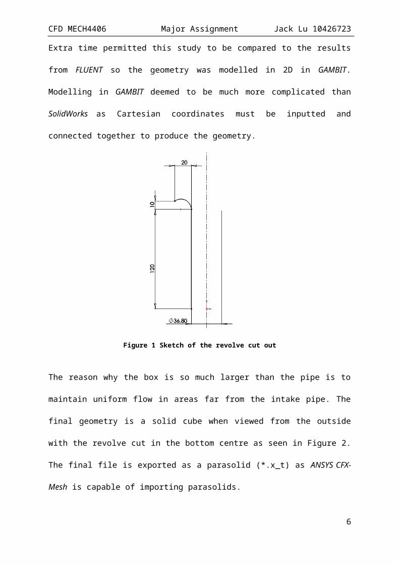
Extra time permitted this study to be compared to the results from FLUENT so the geometry

was modelled in 2D in GAMBIT. Modelling in GAMBIT deemed to be much more

complicated than SolidWorks as Cartesian coordinates must be inputted and connected

together to produce the geometry.

4


Figure 1 Sketch of the revolve cut out

The reason why the box is so much larger than the pipe is to maintain uniform flow in areas

far from the intake pipe. The final geometry is a solid cube when viewed from the outside

with the revolve cut in the bottom centre as seen in Figure 2. The final file is exported as a

parasolid (*.x_t) as ANSYS CFX-Mesh is capable of importing parasolids.

Figure 2 Geometry model of the CFD fluid domain

5


3.0 CFD MESHING

In order to calculate the fluid flow within the domain to a reasonable accuracy, a good quality

mesh needs to be constructed. If the mesh is too fine it will result in a much higher

computational time than needed to achieve the same results if the flow is simple. The first

step in CFD meshing is to import the parasolid file into ANSYS CFX-MESH. CFX-Mesh

utilises a tetrahedral mesh seen in Figure 3 for the mesh construction. This type of mesh is

totally unstructured and is capable of evenly distributing cell spacing in areas where the flow

insignificant (far away from the detail) and compacting cell spacing in areas of high detailed

flow (near boundary layers). The advantage of having this type of unstructured mesh is that it

allows for maximum flexibility in matching mesh cells with the boundary surfaces and for

putting cells where you want them (Anderson 1995). The only length scale mesh control

employed in this study is the body spacing and face spacing controls which is discussed in

Section 3.2.

Figure 3 Triangular surface mesh

3.1 Defining Regions

2D Regions in the model are defined in CFX-Mesh for the location of a meshing feature.

There are three main regions of concern for this type of model. The first is the ‘air region’

6


that is situated on all six faces of the cube and second is the ‘port region’ which is the

circular face situated on the underside of the cube. CFX-Mesh initially defines all faces in the

model as a ‘Default 2D Region’ until the user has manually defined a face as a 2D region.

This means that the last region of concern being the walls of the pipe is left under the title of

‘Default 2D Region’.

3.2 Mesh Sizing

3.2.1 Body Spacing

The body spacing controls the mesh length scale of the volume. It is the initial length scale

before any face spacing or any other length scale control is applied. There is only one

parameter in this option which is the maximum (body) spacing allowed. For this study a

maximum body spacing of 15mm was chosen to achieve a fine mesh for more accurate

results. More refined body spacing would lead to a higher computing time and since the flow

being modelled is considered simple the 15mm maximum spacing seemed reasonable.

3.2.2 Face Spacing

The face spacing controls the mesh length scale on a face (or faces) and in the volume

adjacent to that face. There are four types of face spacing that can be chosen and for this

model angular resolution was chosen.

a. Angular Resolution

b. Relative Error

c. Constant

d. Volume Spacing

Edge lengths on particular faces can be varied upon the local curvature using the angular

resolution face spacing type. This allows for shorter edges to be used upon highly curved

faces and longer edges on flatter surfaces. It is controlled by the Angular Resolution

7


parameter which will determine φ in Figure 4. For this study an angular resolution of 15o is

employed due to the high amount of curvature in the model’s geometry.

Figure 4 Angular Resolution node spacing based upon angle φ (ANSYS 2007)

The next step in the face spacing step is to set the minimum and maximum edge lengths.

These are the minimum and maximum edge lengths of the triangle meshes and ultimately

define the mesh cell size. Again the smaller the cells the higher the computational time

required can be and the larger it is a more inaccurate solution can result. The minimum edge

length for this study is set to 0.5mm whereas the maximum was set to 15mm. A larger

minimum length could have been set to achieve the same results but even with the 0.5mm

minimum length the difference in computational time required was not of great deal.

3.3 Creating the Mesh

Once the regions were defined and the mesh spacing set the mesh is ready to be created. A

surface mesh can be previewed to ensure that the mesh size is adequate for the simulation by

selecting the ‘Generate the surface mesh for the current problem’ button under the CFX-

Mesh main toolbar. When ready the complete volume mesh can be created as a *.gtm file by

selecting ‘Generate volume mesh for the current problem’ button.

The final mesh produces approximately 420 000 elements across all of the meshes produced

for the different bellmouths in this study. Calculating time for each simulation was

approximately 20 minutes each which is considered reasonable for the refined mesh created.

8


For FLUENT a mesh was created in GAMBIT and like ANSYS CFX-Mesh has an advantage in

the refinement of the mesh and in this case, a higher density of triangle cells was placed in

areas of interest as seen in Figure 5. The only trade off is the user-friendly interface that CFX-

Mesh holds but GAMBIT seems to be a much more powerful tool if utilised properly.

Figure 5 Refined mesh allowed higher density of triangles in the areas of higher detail

9


4.0 CFD MODELLING IN CFX-PRE

To set up the simulation CFX-Pre is employed to define the properties of the flow. To begin

the mesh is imported into CFX-Pre as an assembly using the Quick Setup option in CFX-Pre.

The convergence criteria can be set to default as it is sufficient to provide solutions for the

simple simulation. The simulation properties that were modified from default are explained

below.

4.1 Domain

The Domain options allow the user to edit the domain, type of domain, fluid, reference

pressure and other options. The domain that was imported is a fluid domain that is defined as

air at 25oC. In the UWA Motorsport plenum air temperatures are slightly higher due to heat

transfer from the combustion chamber but for the sake of simplification air properties at 25oC

are suffice. The reference pressure is left at 1atm as this simulates external atmospheric

conditions.

4.2 Physics

4.2.1 Simulation Type

In the UWA Motorsport intake plenum pressure waves in transient conditions complicate the

simulation so to keep the simulation simple the simulation type was chosen to be steady state

as we are only interested in the flow occurring around the bellmouth.

4.2.2 Fluid Models

No heat transfer model is selected again to reduce the number of calculations needed. The

turbulence model selected by default was the k-Epsilon model as it is suffice to produce the

results needed in this simulation. Again for the sake of simplicity, other options were left to

default.

10


4.3Boundary Conditions

Three boundary conditions were set for this simulation and are explained below.

4.3.1 Air Opening Boundary Condition

The air boundary is linked to the ‘air region’ and is set to an opening with a relative pressure

of -20kPa. The opening type was selected over inlet type because it allowed air to flow both

ways as it if were open to atmosphere to ensure uniform flow occurs away from the intake

pipe. The relative pressure of -20kPa is used to simulate the internal plenum pressure when

the engine is operating at low speeds. The turbulence intensity remained default at 5% as

we’re trying to maintain a constant flow in areas away from the pipe.

4.3.2 Outlet Boundary Condition

The outlet boundary condition is linked to the ‘port region’ and is set as an outlet with an

average static relative pressure of -80kPa. This relative pressure is an average over the whole

outlet to allow for any variations. -80kPa was chosen as an estimation using the compression

ratio of the engine (12:1) with the consideration of valve overlap. It is important to note that it

is set as a subsonic outlet but in reality velocities are capable of reaching or exceeding Mach1

within the runners of the intake plenum particularly at higher engine speeds.

4.3.3 Physical Boundary Condition

If no other region is set as a boundary condition manually, CFX-Pre sets it as a physical no

slip smooth wall boundary condition by default which is good enough for this simulation.

4.4 Write to Solver

Once all preliminary settings were defined the simulation can begin first by saving the CFX-

Pre definitions as a *.def file that can be read by the solver.

The FLUENT simulation was set up with the same parameters as that of ANSYS CFX-Pre

above.

11


5.0 CFD SOLVING IN CFX-SOLVER

Once the definition file has been loaded, the solver is capable of solving the simulation.

The solver uses the Navier-Stokes equation which are:

Continuity (conservation of mass)

Momentum (non-conservation form)

For this simulation, it took approximately 20 minutes over 56 iterations to complete

producing an output file with the simulation’s log and plots an updated residuals graph seen

in Figure 6.

FLUENT took approximately 30 seconds to solve the 2D case with 144 iterations and the

residual plot can be seen in Figure 7. The time taken in FLUENT is far less than ANSYS CFX

as FLUENT only analyses the 2D case.

12


Figure 6 CFX-Solver Output with residual graph on the left and process log on the right

Figure 7 Residual plot from FLUENT 6

13


6.0 CFD ANALYSIS IN CFX-POST

CFX-Solver also puts out a results file in the form of *.res in which requires CFX-Post to

open. In CFX-Post a plane is created upon the XY plane so that contour plots can be created.

Contour plots provide a good indication of what is occurring as the bellmouth geometry is

symmetrical 360o all around the vertical axis. It is important to note when comparing colour

contour plots, the legends need to be standardised so that a true comparison can be observed

between candidates.

6.1 Straight Pipe Intake

The first case investigated was the straight pipe intake and using CFX-Post a velocity vector,

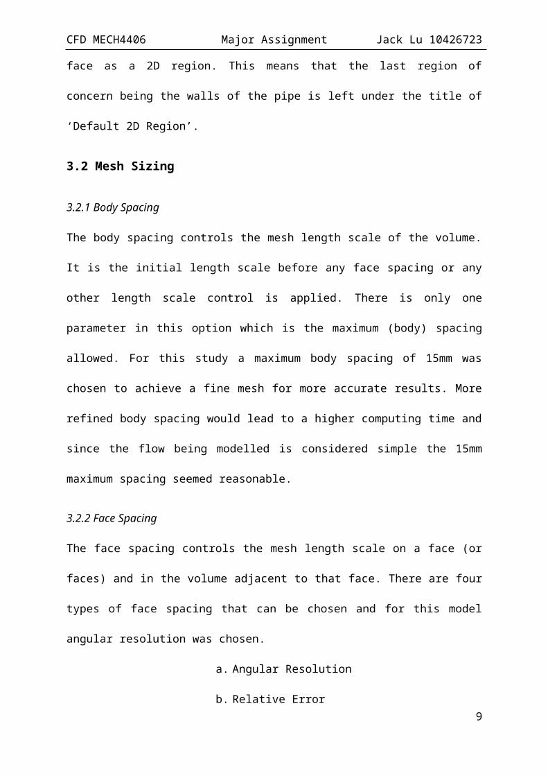
u-velocity, and pressure contour plot were taken. The outline in Figure 8 shows flow

separation and some circulation occurring as U-velocities pass around the straight bend. Flow

separation is not sort after because the flow becomes detached from the surface of the object

and instead takes form of eddies and vortices which can restrict flow (Ravinder & Prasad

2006). Note that as predicted earlier, the maximum velocity achieved through the pipe is

358m/s, which is greater than Mach1 approximately 20mm downstream from the entry.

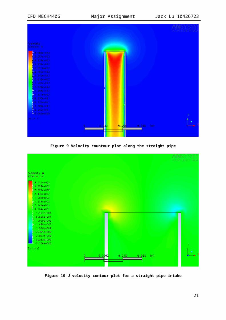
The U-velocity plot in Figure 10 shows high velocities at the tip of the pipe which can be

used to explain the flow separation occurring 20mm below it. The straight pipe is

experiencing a maximum horizontal velocity of 198m/s and this velocity must be greatly

reduced to prevent flow separation from occurring.

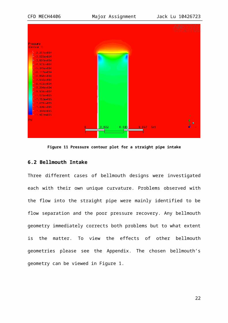
Lastly the pressure plot in Figure 11 shows poor pressure recovery from the sudden

contraction. It shows the pressure slowly increasing downstream of the pipe from the huge

pressure drop located on the walls of the entry of the pipe. This means that a longer runner

14


length will be needed for pressure recovery and this may not be ideal in terms of packaging

or ideal for tuned runner lengths.

Figure 8 Velocity contour plot with velocity vectors for a straight pipe intake

Figure 9 Velocity countour plot along the straight pipe15


Figure 10 U-velocity contour plot for a straight pipe intake

Figure 11 Pressure contour plot for a straight pipe intake

16


6.2 Bellmouth Intake

Three different cases of bellmouth designs were investigated each with their own unique

curvature. Problems observed with the flow into the straight pipe were mainly identified to be

flow separation and the poor pressure recovery. Any bellmouth geometry immediately

corrects both problems but to what extent is the matter. To view the effects of other

bellmouth geometries please see the Appendix. The chosen bellmouth’s geometry can be

viewed in Figure 1.

Flow separation problems no longer exists as seen in Figure 12 which immediately reduces

the likelihood of creating eddies and assists in the sought after laminar flow within the pipe.

This result is reinforced with a re-run of the simulation in FLUENT producing a velocity

vector plot seen in Figure 16. The U-velocity plot in Figure 14 also shows a large velocity

reduction in the horizontal plane which further reinforces the relationship between the U-

velocity and flow separation in this case as there was no flow separation present.

Secondly the maximum velocities experienced at the entry of the intake pipe has significantly

reduced from 358m/s to 290m/s and overall downstream of the pipe, remains quite constant

whereas the straight pipe dramatically loses its velocity to approximately 270m/s. In terms of

engine performance, this will play a large factor in increasing the engines volumetric

efficiency as higher velocities will mean a higher momentum since momentum p=mv.

The pressure recovery from the bellmouth design is seen to be a large improvement over that

of the straight pipe (see Figure 15). A large drop in pressure occurs on the side walls of the

pipe just as the cross sectional area of the pipe dramatically reduces. Pressures become

uniform approximately 10mm downstream from that area compared to the gradual pressure

17


changes along the straight pipe which explains the much more laminar flow experienced in

Figure 12.

The velocity magnitude outputted by FLUENT identified from the vectors colour in Figure 16

shows a slight disagreement in the velocity as it is seen to have a slightly higher magnitude in

the areas of low pressure seen in ANSYS’ pressure plot of Figure 15. This is believed to be

the correct case as it is expected a velocity increase in areas of low pressure.

Figure 12 Velocity contour plot with velocity vectors showing no sign of flow separation

18


Figure 13 Velocity contour plot along the bellmouth pipe

Figure 14 U-velocity plot showing reduced velocities in the horizontal plane

19


Figure 15 Pressure contour plot showing constant pressure within the pipe

Figure 16 FLUENT velocity vectors shows similar results to ANSYS CFX

20


CONCLUSION

The results seen were expected in terms of the improvements by implementing the bellmouth

but from this study I have gained a better understanding why. The effect of employing this

geometry decreases the U-velocities (in the horizontal plane) at the intake and reduces or

eliminates flow separation. This produces an improved laminar flow downstream of the pipe

through better pressure recovery compared to that of the straight pipe.

I have also gained a better understanding of how CFD operates and what parameters were

important to be able to simulate and analyse a simple geometry. It has increased my

confidence in the ability to comprehend the effects of geometries on fluid flow and therefore

assist in my designs for the intake of the UWA Motorsport car. I have also learnt a great deal

on how to use the ANSYS and FLUENT packages for the study of CFD.

If there were more time, further studies could be allocated to the effects of implementing the

bellmouths on all four runners within a plenum to see further improvements. Because the

intake of the UWA Motorsport car draws air from a 20mm restrictor, it is wise to use CFD to

analyse the relationship between cylinder filling and the position of the 20mm restrictor.

Other ideas include a vector analysis within the plenum to reduce any recirculation by adding

baffles. There are so many possibilities in which CFD can become such a useful tool for and

as long as the parameters are set up correctly, it is definitely a powerful tool in design.

21


REFERENCES

Anderson, J.D. 1995, Computational fluid dynamics : the basics with applications, McGraw-Hill, New York.

ANSYS CFX 2005, ANSYS CFX 10.0 Help Files, ANSYS Inc.

O’Neill, P. & Rasnasinghe J. 2007, Computational Fluid Dynamics lectures, lecture notes taken from MECH4406 at The University of Western Australia School of Mechanical Engineering, Crawley in Semester 1 2007.

Ravinder, Y. & Prasad, N. 2006, Optimization of Intake System and Filter of an Automobile using CFD Analysis, MNR Filters, India

22


APPENDIX

APPENDIX Bellmouth A

23


24


APPENDIX Bellmouth B

25


26

members.iinet.net.aumembers.iinet.net.au/~phlu/word/CFD Major Assignment.doc · Web viewThe use...

Documents

Transcript of members.iinet.net.aumembers.iinet.net.au/~phlu/word/CFD Major Assignment.doc · Web viewThe use...