Statistical Causality

Philip DawidStatistical Laboratory

University of Cambridge

Statistical Causality

1. The Problems of Causal Inference2. Formal Frameworks for Statistical Causality3. Graphical Representations and Applications4. Causal Discovery

1. The Problems of Causal Inference

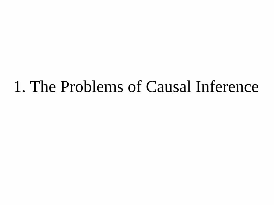
Conceptions of Causality

• Constant conjunction– Deterministic

• Mechanisms– “Physical” causality

Agency– Effects of actions/interventions

Contrast– Variation of effect with changes to cause

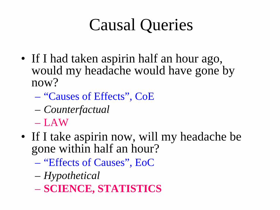
Causal Queries

• If I had taken aspirin half an hour ago, would my headache would have gone by now? – “Causes of Effects”, CoE– Counterfactual– LAW

• If I take aspirin now, will my headache be gone within half an hour?– “Effects of Causes”, EoC– Hypothetical– SCIENCE, STATISTICS

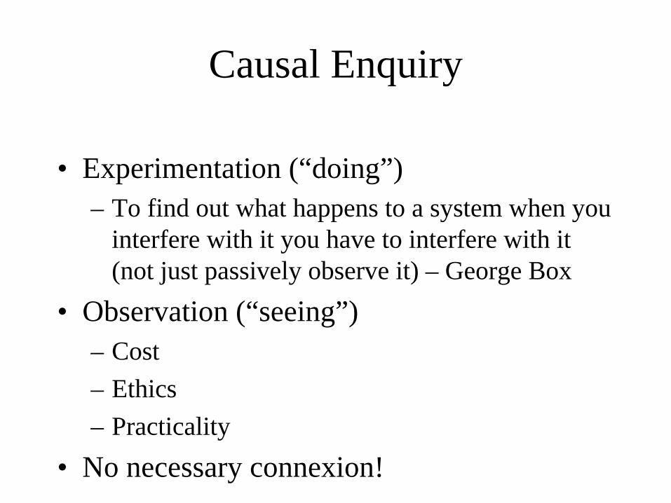
Causal Enquiry

• Experimentation (“doing”)– To find out what happens to a system when you

interfere with it you have to interfere with it (not just passively observe it) – George Box

• Observation (“seeing”)– Cost– Ethics– Practicality

• No necessary connexion!

Problems of observational studies

An observed association between a “cause”and an “effect” may be spurious:

– Reverse causation– Regression to mean– Confounding

• common cause• differential selection

– …

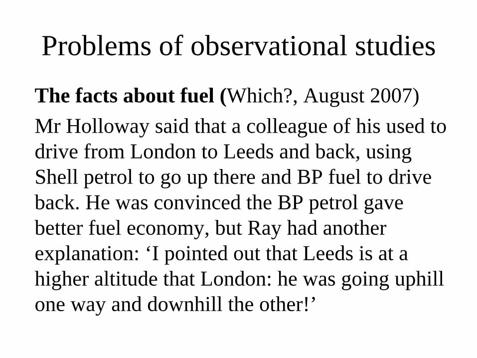
Problems of observational studiesThe facts about fuel (Which?, August 2007)Mr Holloway said that a colleague of his used to drive from London to Leeds and back, using Shell petrol to go up there and BP fuel to drive back. He was convinced the BP petrol gave better fuel economy, but Ray had another explanation: ‘I pointed out that Leeds is at a higher altitude that London: he was going uphill one way and downhill the other!’

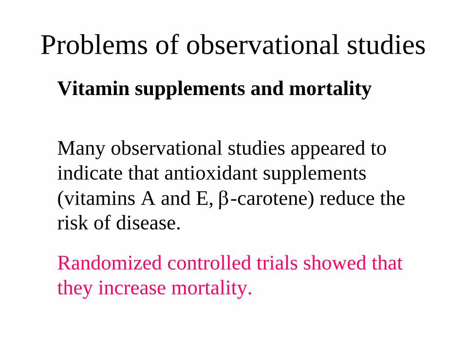
Problems of observational studiesVitamin supplements and mortality

Many observational studies appeared to indicate that antioxidant supplements (vitamins A and E, -carotene) reduce the risk of disease.

Randomized controlled trials showed that they increase mortality.

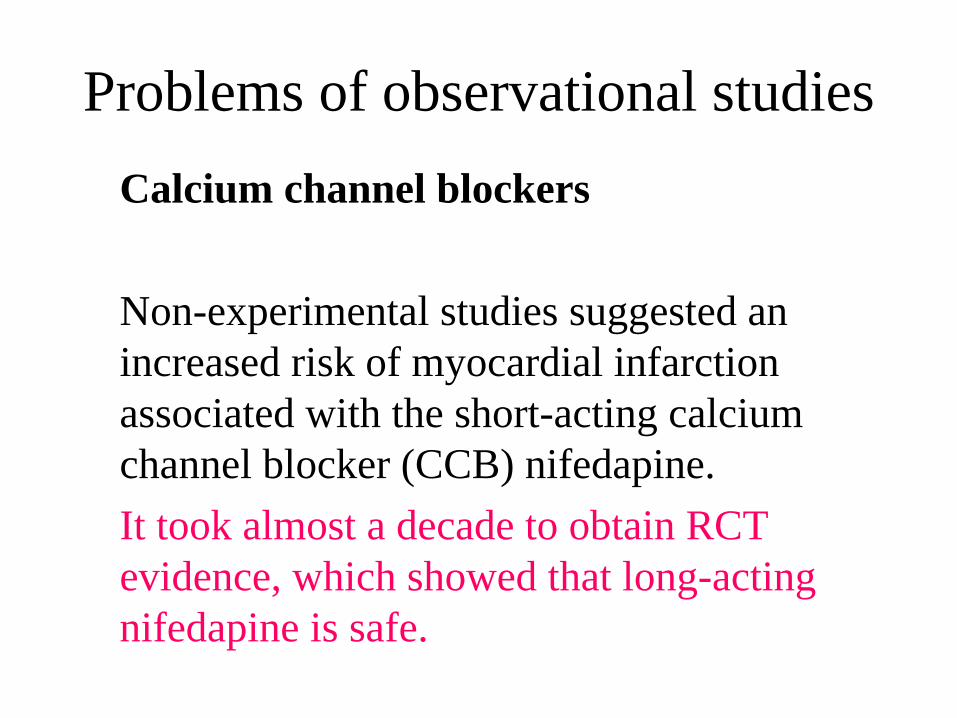
Problems of observational studiesCalcium channel blockers

Non-experimental studies suggested an increased risk of myocardial infarction associated with the short-acting calcium channel blocker (CCB) nifedapine. It took almost a decade to obtain RCT evidence, which showed that long-acting nifedapine is safe.

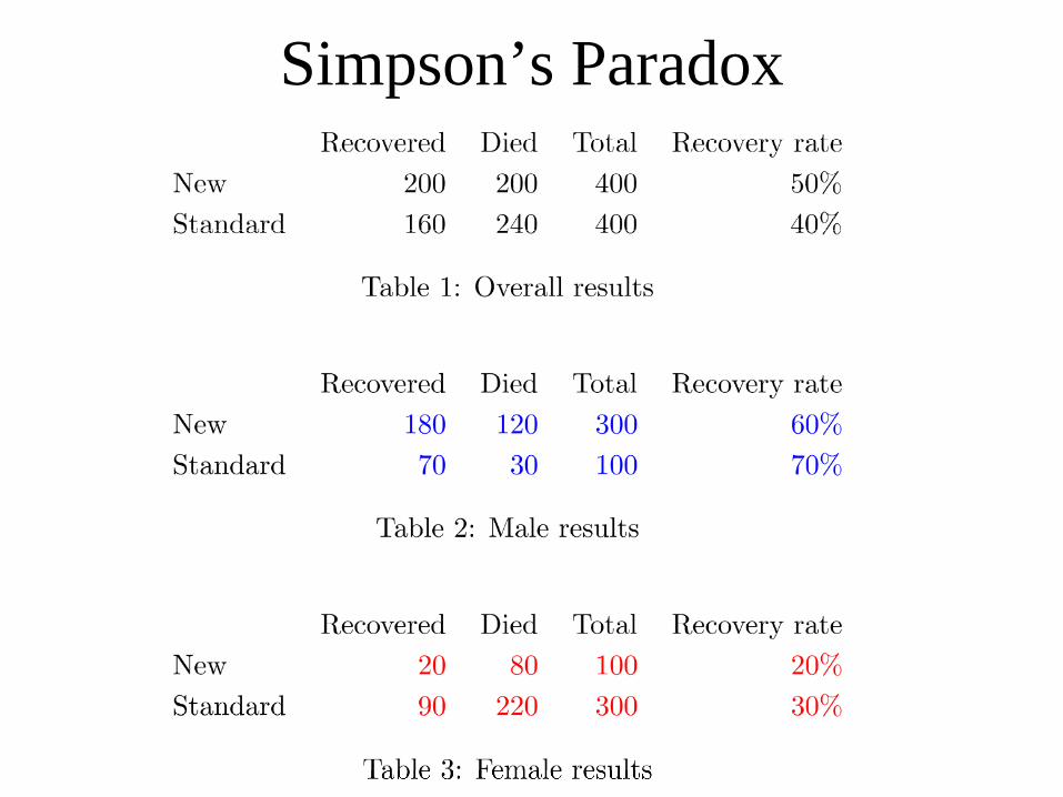
Simpson’s Paradox

Causal Inference

• Association is not causation!• Traditionally, Statistics dealt with association

– Theory of Statistical Experimental Design and Analysis does address causal issues

• but of no real use for observational studies

• How to make inferences about causation?– “bold induction”, to a novel context

• Do we need a new formal framework?

2. Formal Frameworks for Statistical Causality

Some Formal Frameworks

• Structural equations• Path diagramsDirected acyclic graphs• …

Probability distributions• Potential responses• Functional relationshipsExtended conditional independence• …

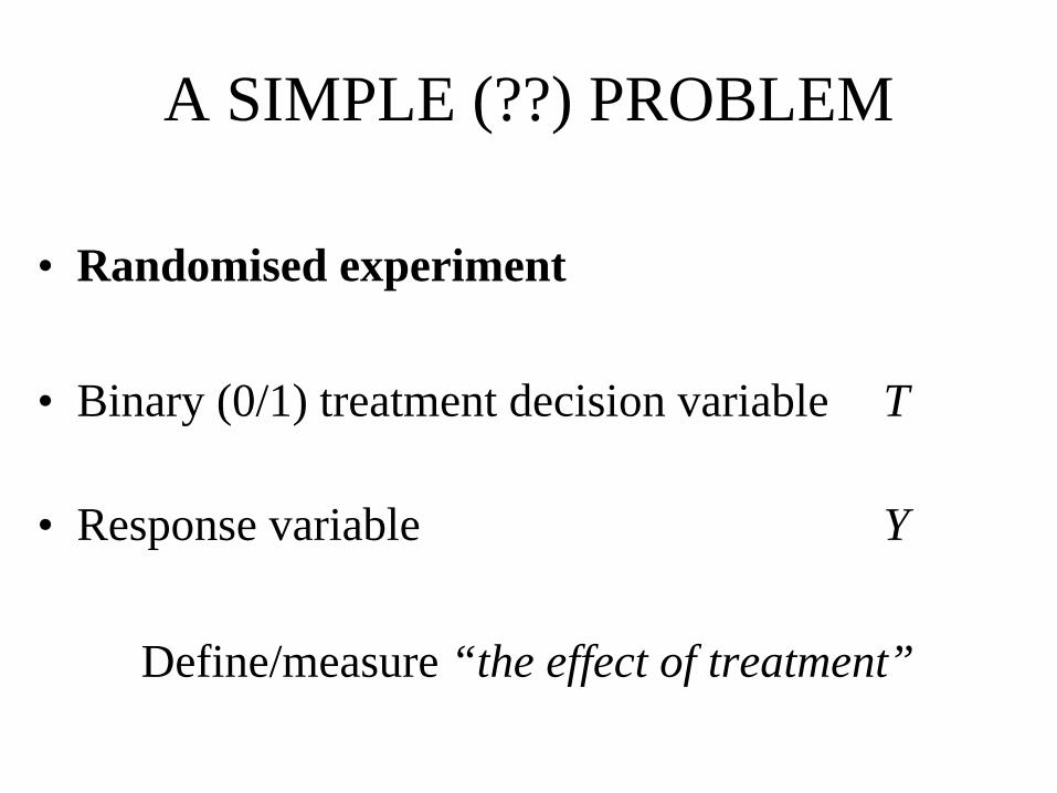
A SIMPLE (??) PROBLEM

• Randomised experiment

• Binary (0/1) treatment decision variable T

• Response variable Y

Define/measure “the effect of treatment”

Probability Model

• Measure effect of treatment by change in the distributionof Y: compare P0 and P1

– e.g. by change in expected response: = 1 0 (average causal effect, ACE)

• Specify/estimate conditional distributionsPt for Y given T = t (t = 0, 1)

• Probability model all we need for decision theory– choose t to minimise expected loss EY ∼ Pt

{L(Y)}

(Fisher)

[e.g. N(t, 2) ]

T

Decision Tree

0

1

y

y

Y

Y

Y~P0

Y~P1

L(y)

L(y)

Influence Diagram

T YY | T=t ~ Ptt

LL(y)

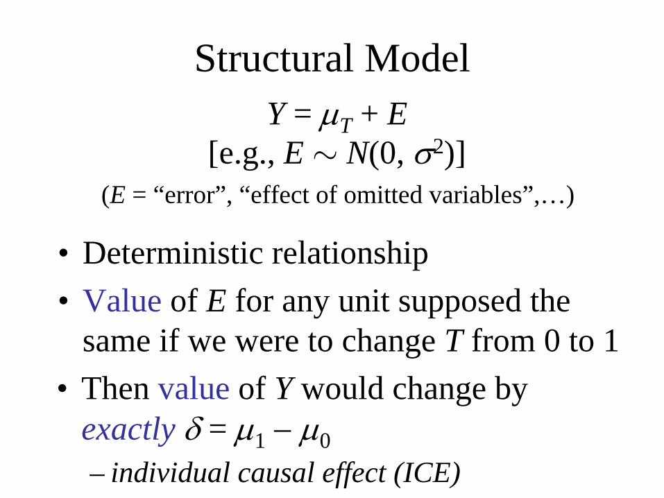
• Then value of Y would change by exactly = 1 0

Structural Model

• Deterministic relationship• Value of E for any unit supposed the

same if we were to change T from 0 to 1

– individual causal effect (ICE)

(E = “error”, “effect of omitted variables”,…)

Y = T + E[e.g., E ∼ N(0, 2)]

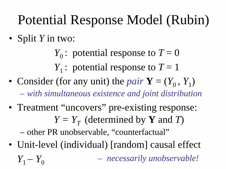
• Split Y in two:Y0 : potential response to T = 0Y1 : potential response to T = 1

Potential Response Model (Rubin)

– necessarily unobservable!

• Consider (for any unit) the pair Y = (Y0 , Y1)– with simultaneous existence and joint distribution

• Treatment “uncovers” pre-existing response:Y = YT (determined by Y and T)

– other PR unobservable, “counterfactual”• Unit-level (individual) [random] causal effect

Y1 Y0

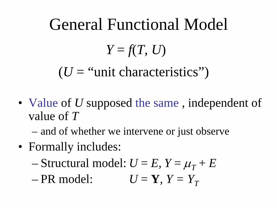
General Functional Model

• Value of U supposed the same , independent of value of T– and of whether we intervene or just observe

• Formally includes:– Structural model: U = E, Y = T + E– PR model: U = Y, Y = YT

(U = “unit characteristics”)Y = f(T, U)

• Any functional model Y = f(T, U) generates a PR model: Yt = f(t, U)

• Any PR model generates a probability model:Pt is marginal distribution of Yt (t = 0, 1)

• Distinct PR models can generate the samestatistical model– e.g., correlation between Y0 and Y1 arbitrary

• Cannot be distinguished observationally• Can have different inferential consequence

– can be problematic!

Potential Response Model

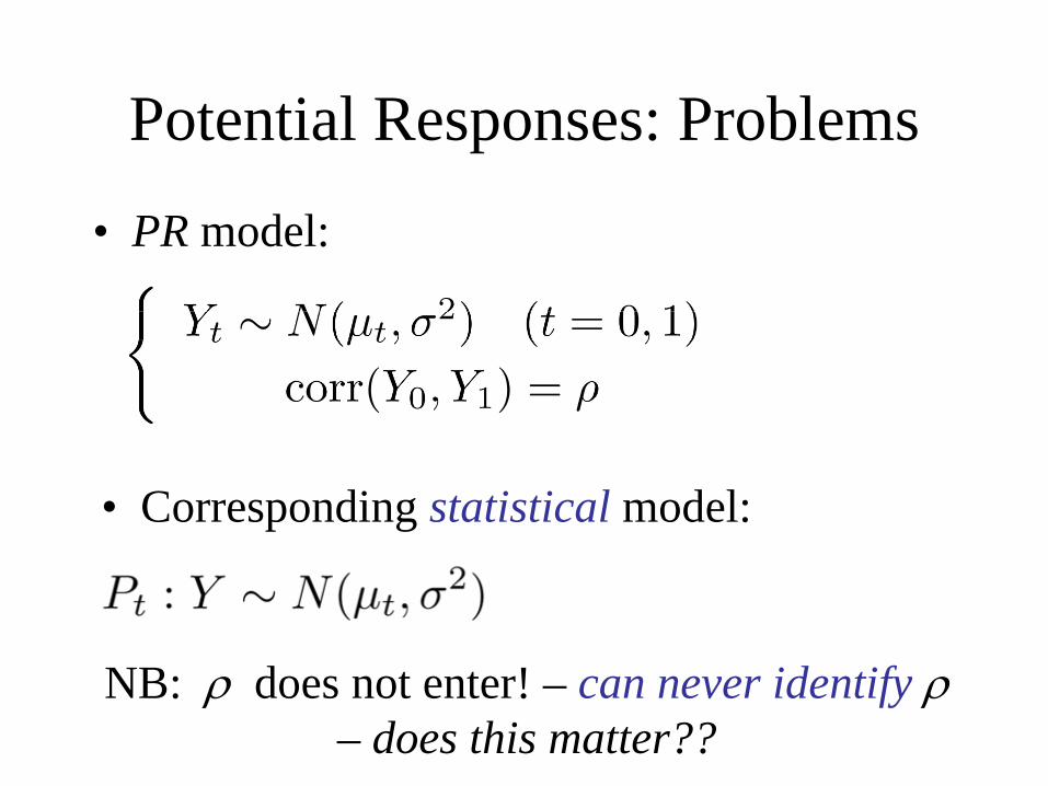
Potential Responses: Problems

NB: does not enter! – can never identify – does this matter??

• Corresponding statistical model:

• PR model:

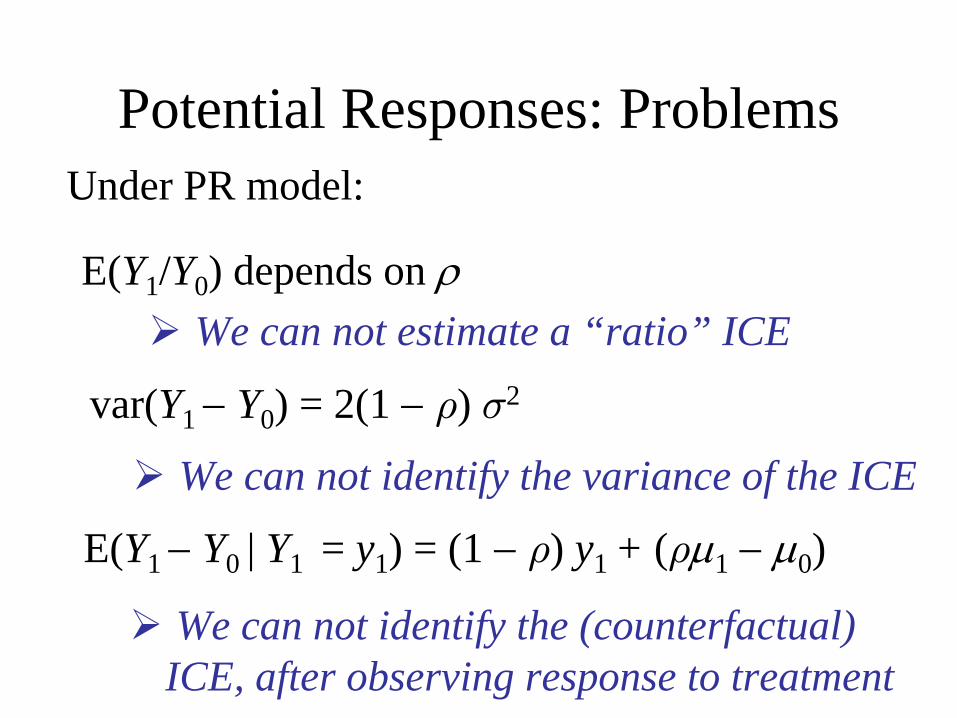
Potential Responses: ProblemsUnder PR model:

We can not identify the variance of the ICE

We can not identify the (counterfactual) ICE, after observing response to treatment

E(Y1/Y0) depends on We can not estimate a “ratio” ICE

var(Y1 Y0) = 2(1 ρ) σ2

E(Y1 Y0 | Y1 = y1) = (1 ρ) y1 + (ρ1 0)

OBSERVATIONAL STUDY

• Treatment decision taken may be associated with patient’s state of health

• What assumptions are required to make causal inferences?

• When/how can such assumptions be justified?

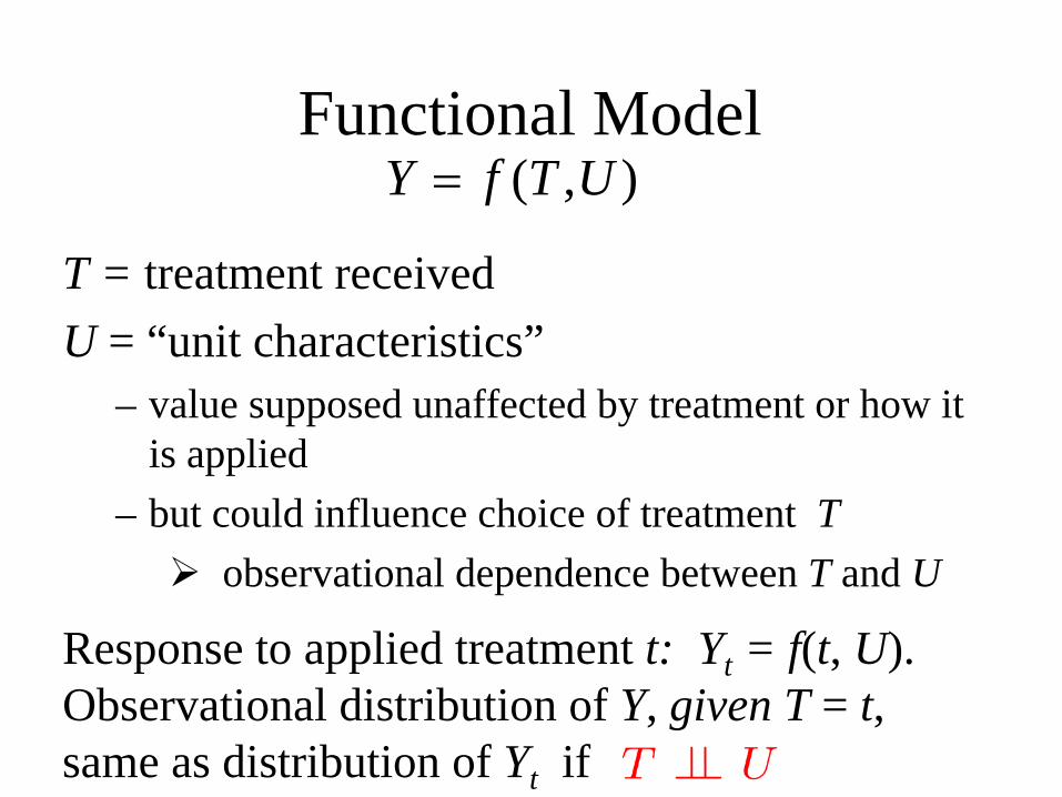
Functional Model

T = treatment receivedU = “unit characteristics”

– value supposed unaffected by treatment or how it is applied

– but could influence choice of treatment T observational dependence between T and U

),( UTfY

Response to applied treatment t: Yt = f(t, U).Observational distribution of Y, given T = t, same as distribution of Yt if

T Y

U

Functional Model

U = “unit characteristics”– value supposed unaffected by treatment or how it

is applied– but could influence treatment choice

),( UTfY

UPU ~

T Y

U

Functional Model

“No confounding” (“ignorable treatment assignment”) if

(treatment independent of “unit characteristics”)

T ⊥⊥ U

TPT ~ ),( UTfY

UPU ~

T Y

Y

“No confounding” (“ignorable treatment assignment”) if

(treatment independent of potential responses)

TPT ~

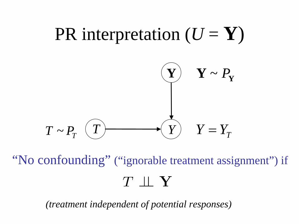
PR interpretation (U = Y)

TYY

YY P~

PR interpretation (U = Y)

• Value of Y = (Y0, Y1) on any unit supposed the same in observational and experimental regimes, as well as for both choices of T

• No confounding: independence of Tfrom PR pair Y

How are we to judge this??

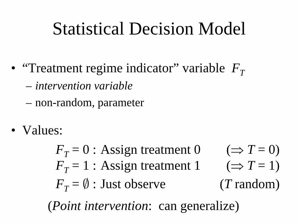
• “Treatment regime indicator” variable FT– intervention variable– non-random, parameter

• Values:FT = 0 : Assign treatment 0 ( T = 0)FT = 1 : Assign treatment 1 ( T = 1)FT = ∅ : Just observe (T random)

Statistical Decision Model

(Point intervention: can generalize)

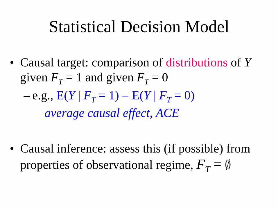
• Causal target: comparison of distributions of Ygiven FT = 1 and given FT = 0– e.g., E(Y | FT = 1) E(Y | FT = 0)

average causal effect, ACE

• Causal inference: assess this (if possible) from properties of observational regime, FT = ∅

Statistical Decision Model

True ACE is

E(Y | T = 1, FT = 1) E(Y | T = 0, FT = 0)Its observational counterpart is:

E(Y | T = 1, FT = ∅) E(Y | T = 0, FT = ∅)“No confounding” (ignorable treatment assignment)

when these are equal.

Can strengthen:p(y | T = t, FT = 1) = p(y | T = t, FT = ∅)

distribution of Y | T the same in observational and experimental regimes

Statistical Decision Model

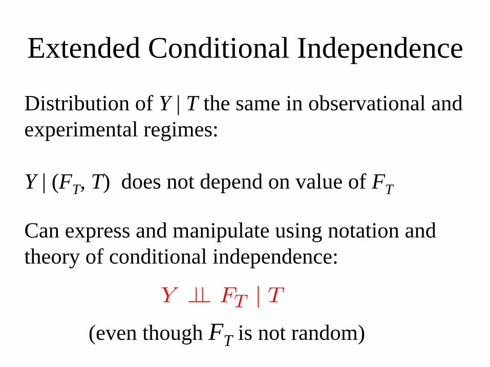
Extended Conditional Independence

Distribution of Y | T the same in observational and experimental regimes:

Y | (FT, T) does not depend on value of FT

Can express and manipulate using notation and theory of conditional independence:

(even though FT is not random)

3. Graphical Representations and Applications

Extended Conditional Independence

Distribution of Y | T the same in observational and experimental regimes:

Y | (FT, T) does not depend on value of FT

Can express and manipulate using notation and theory of conditional independence:

(even though FT is not random)

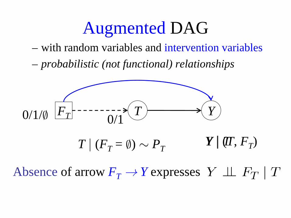
T | (FT = ∅) ∼ PT

TFT Y0/1/∅ 0/1

Y | T

Augmented DAG

Absence of arrow FT → Y expresses

Y | (T, FT)

– with random variables and intervention variables– probabilistic (not functional) relationships

Y

U

TFT

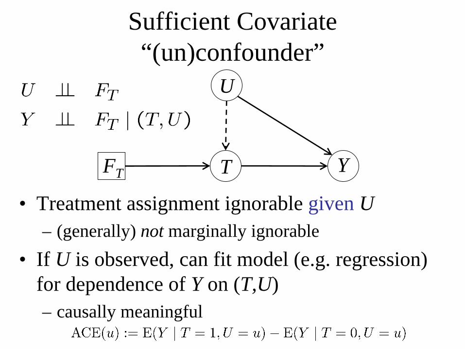
• Treatment assignment ignorable given U– (generally) not marginally ignorable

• If U is observed, can fit model (e.g. regression) for dependence of Y on (T,U)– causally meaningful

Sufficient Covariate“(un)confounder”

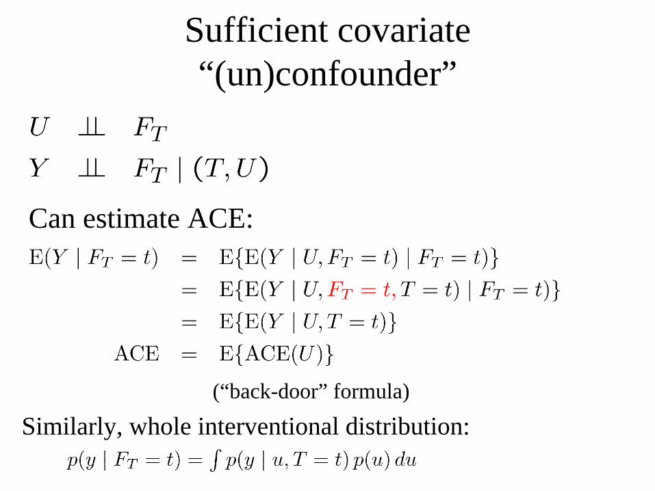
Can estimate ACE:

Similarly, whole interventional distribution:

Sufficient covariate“(un)confounder”

(“back-door” formula)

T Y

U

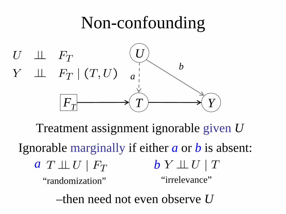
Non-confounding

ab

Ignorable marginally if either a or b is absent:Treatment assignment ignorable given U

FT

a“randomization”

b“irrelevance”

–then need not even observe U

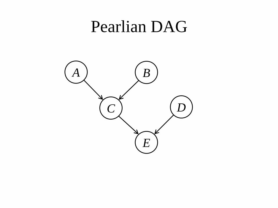
Pearlian DAG

• Envisage intervention on any variable in system

• Augmented DAG model, but with intervention indicators implicit

• Every arrow has a causal interpretation

A B

C D

E

Pearlian DAG

A B

C D

E

FA FB

FC FD

FE

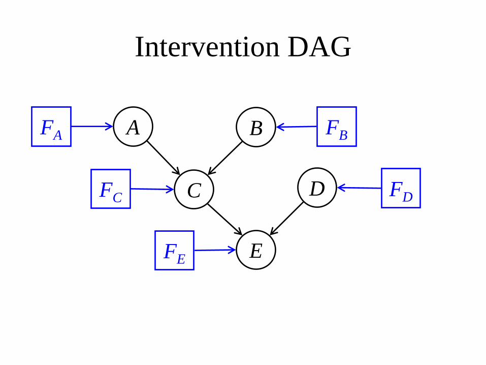
Intervention DAG

Intervention DAGA B

C D

E

FA FB

FC FD

FE

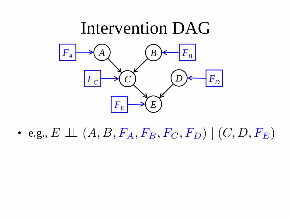
• e.g.,

Intervention DAGA B

C D

E

FA FB

FC FD

FE

• e.g.,• When E is not manipulated, its conditional

distribution, given its parents C, D is unaffected by the values of A, B and by whether or not any of the other variables is manipulated– modular component

More complex DAGs

= treatment strategy

By d-separation:

(would fail if e.g. U → Y)

U

Y

A1

L

A2

(influence diagram)

X

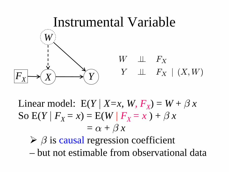
Instrumental Variable

Y

W

FX

W ⊥⊥ FX

Y ⊥⊥ FX | (X,W )

Linear model: E(Y | X=x, W, FX) = W + β xSo E(Y | FX = x) = E(W | FX = x ) + β x

= α + β x β is causal regression coefficient– but not estimable from observational data

X

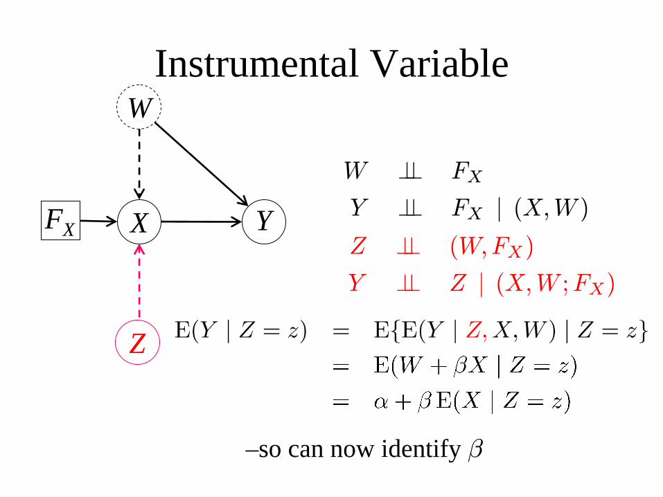
Instrumental Variable

Y

Z

W

FXZ ⊥⊥ (W,FX)

Y ⊥⊥ Z | (X,W ;FX)

W ⊥⊥ FX

Y ⊥⊥ FX | (X,W )

–so can now identify β

X

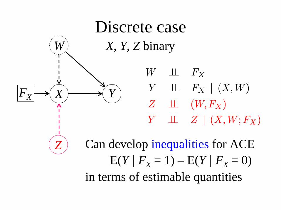
Discrete case

Y

W

FXZ ⊥⊥ (W,FX)

Y ⊥⊥ Z | (X,W ;FX)

W ⊥⊥ FX

Y ⊥⊥ FX | (X,W )

Can develop inequalities for ACEE(Y | FX = 1) – E(Y | FX = 0)

in terms of estimable quantities

X, Y, Z binary

Z

X

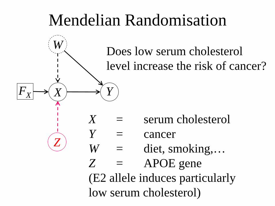
Mendelian Randomisation

Y

W

FX

X = serum cholesterolY = cancerW = diet, smoking,…Z = APOE gene(E2 allele induces particularly low serum cholesterol)

Does low serum cholesterol level increase the risk of cancer?

Z

X

Equivalence

Y

Z

W

FX

Z

X

U

W

YFX

causal?

ZZ

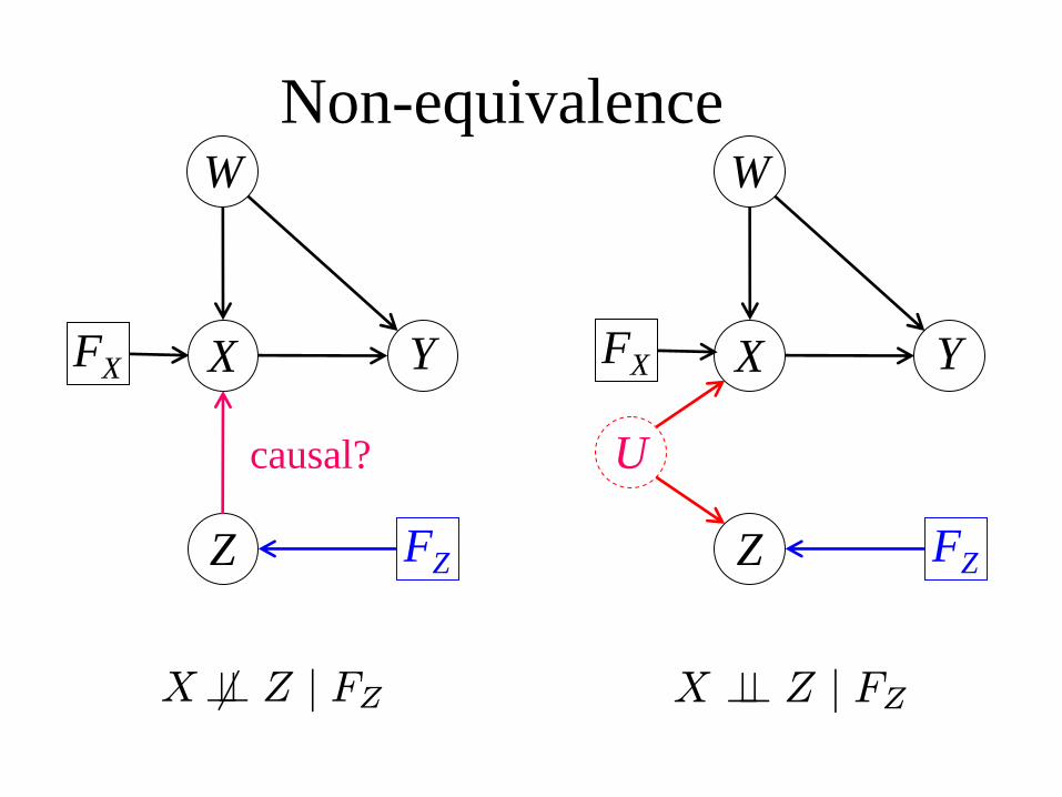
Non-equivalence

X

U

W

YX Y

W

FZ FZ

FX FX

causal?

X 6⊥⊥ Z | FZ X ⊥⊥ Z | FZ

Can we identify a causal effect from observational data?

• Model with domain and (explicit or implicit) intervention variables, specified ECI properties– e.g. augmented DAG, Pearlian DAG

• Observed variables V, unobserved variables U• Can identify observational distribution over V• Want to answer causal query, e.g. p(y | FX = x)

– write as• When/how can this be done?

p(y | x̌)

Example: “back-door formula”

Y

Z

XFX

Z ⊥⊥ FX

Y ⊥⊥ FX | (X,Z)

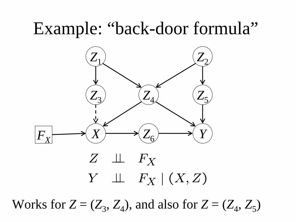
Example: “back-door formula”

Y

Z1

XFX

Z5Z4

Z2

Z3

Z6

Works for Z = (Z3, Z4), and also for Z = (Z4, Z5)

Z ⊥⊥ FX

Y ⊥⊥ FX | (X,Z)

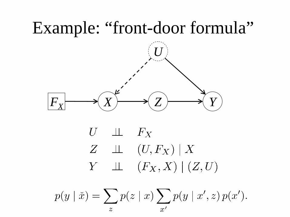
Example: “front-door formula”

ZX

U

YFX

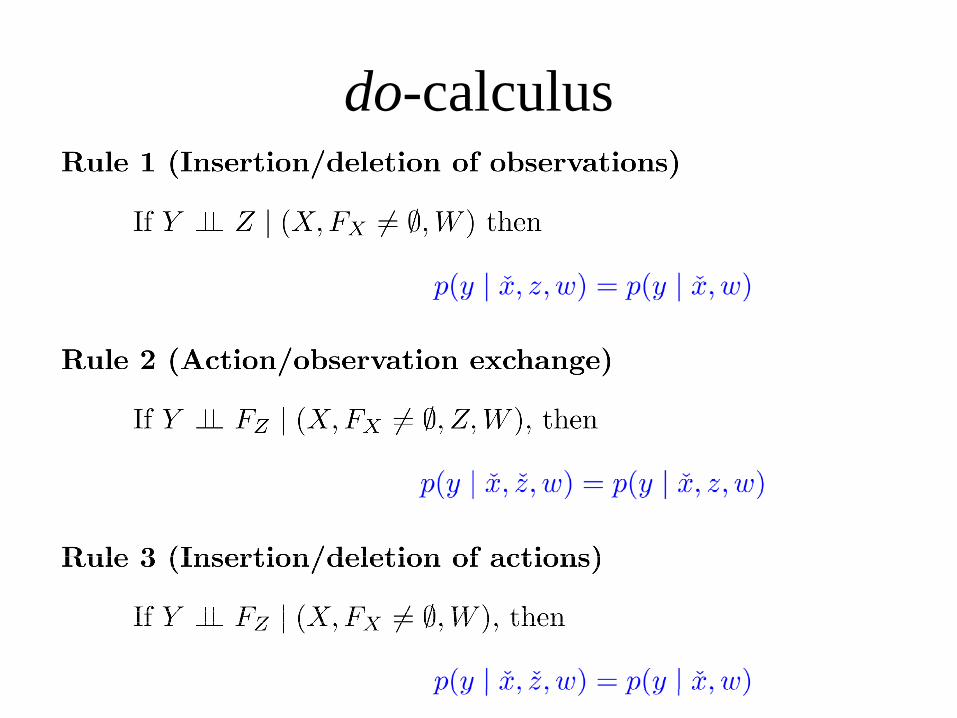
do-calculus

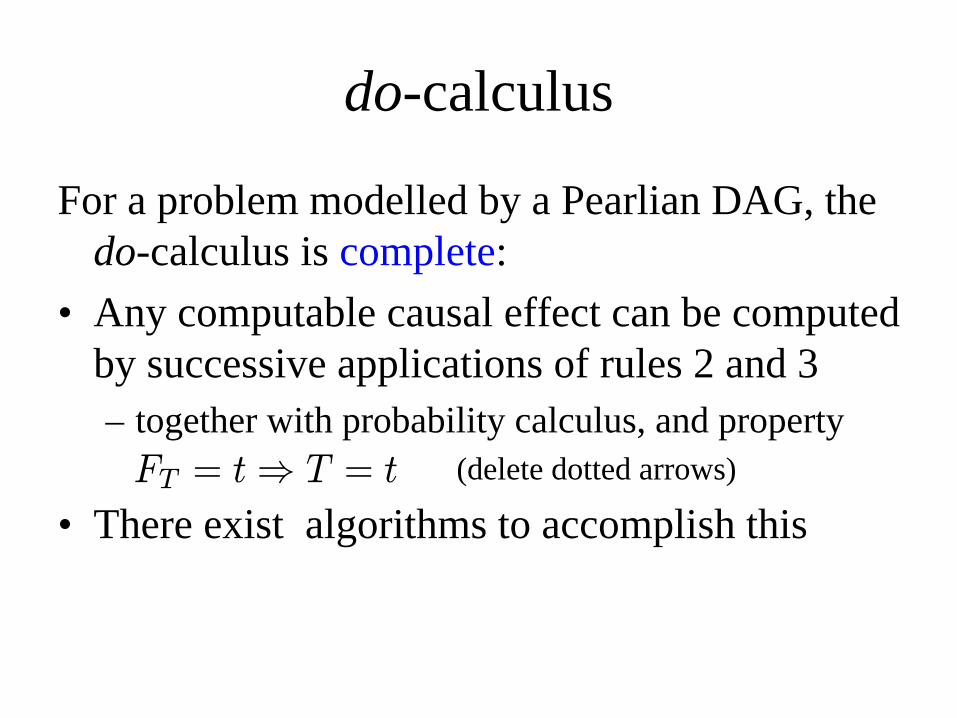
For a problem modelled by a Pearlian DAG, the do-calculus is complete:

• Any computable causal effect can be computed by successive applications of rules 2 and 3– together with probability calculus, and property

» (delete dotted arrows)

• There exist algorithms to accomplish this

do-calculus

FT = t⇒ T = t

4. Causal Discovery

Probabilistic Causality

• Intuitive concepts of “cause”, “direct cause”,…• Principle of the common cause:

“Variables are independent, given their common causes”

• Assume causal DAG representation: – direct causes of V are its DAG parents– all “common causes” included

Probabilistic Causality

CAUSAL MARKOV CONDITION– The causal DAG also represents the observational

conditional independence properties of the variables• WHEN??• WHY??

• CAUSAL FAITHFULNESS CONDITION– No extra conditional independencies

• WHY??

Causal Discovery

• An attempt to learn causal relationships from observational data

• Assume there is an underlying causal DAG(possibly including unobserved variables) satisfying the (faithful) Causal Markov Condition

• Use data to search for a DAG representing the observational independencies model selection

• Give this a causal interpretation

Causal Discovery

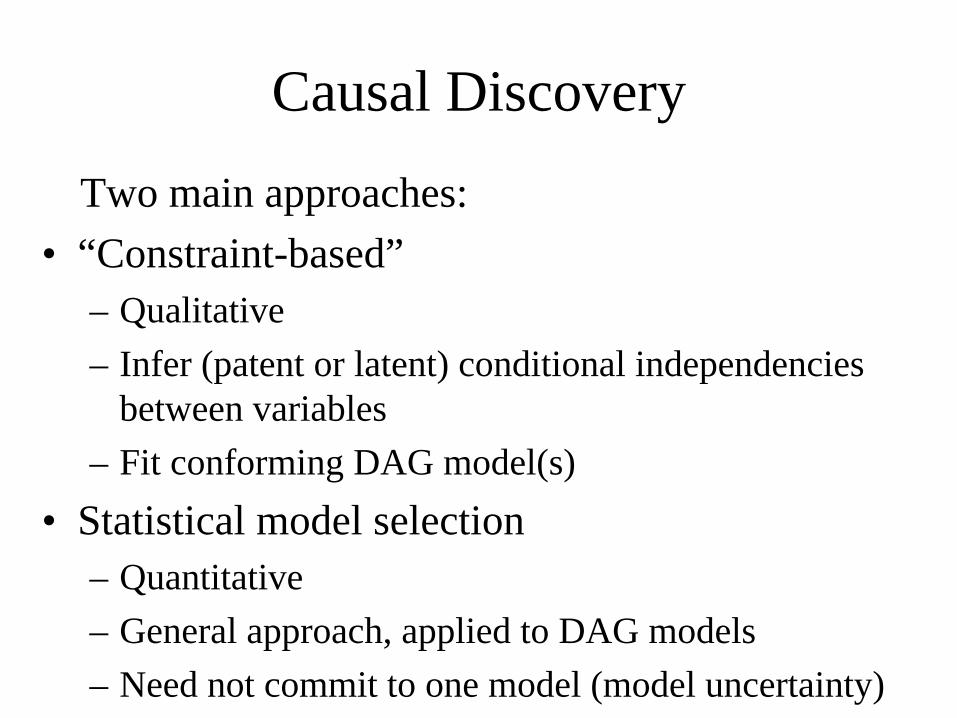
• “Constraint-based”– Qualitative– Infer (patent or latent) conditional independencies

between variables– Fit conforming DAG model(s)

• Statistical model selection– Quantitative– General approach, applied to DAG models– Need not commit to one model (model uncertainty)

Two main approaches:

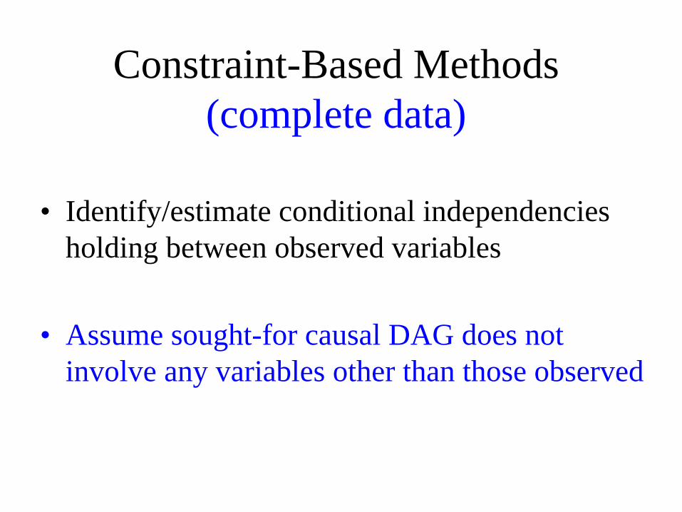
Constraint-Based Methods

• Identify/estimate conditional independencies holding between observed variables

• Assume sought-for causal DAG does not involve any variables other than those observed

(complete data)

Wermuth-Lauritzen algorithm

• Assume variables are “causally ordered” a priori: (V1, V2,…, VN), s.t arrows can only go from lower to

higher• For each i, identify (smallest) subset Si of

Vi-1 := (V1, V2,…, Vi-1) such that

• Draw arrow from each member of Si to Vi

Vi⊥⊥V i−1 | Si

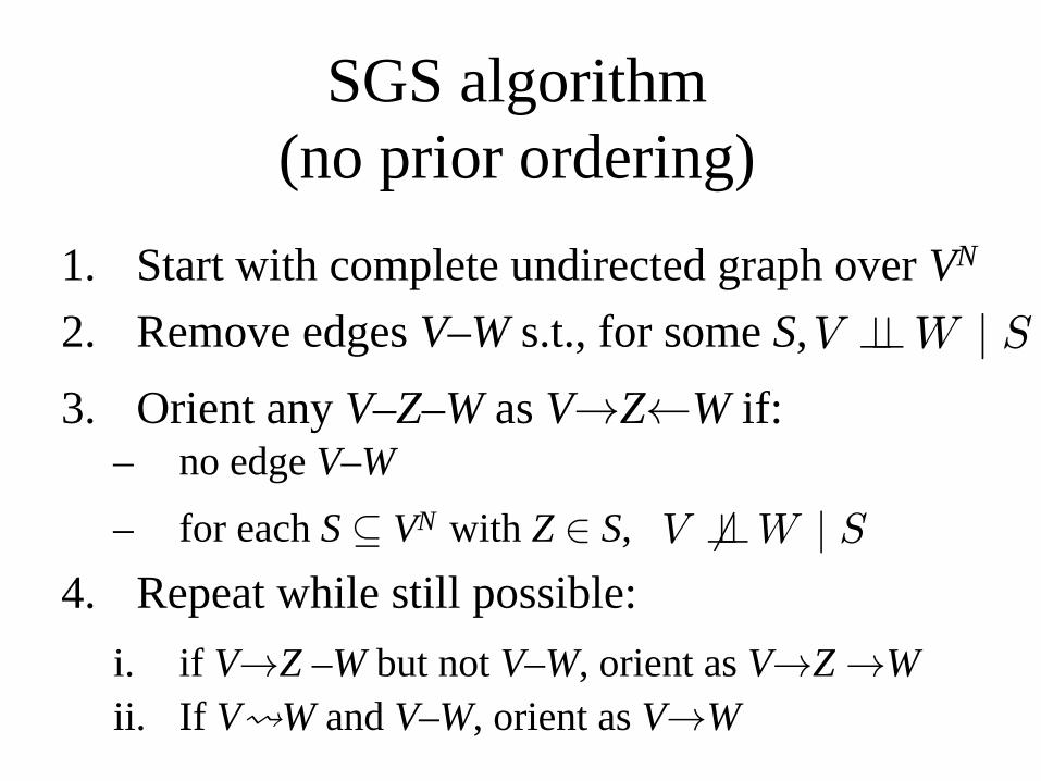
SGS algorithm(no prior ordering)

1. Start with complete undirected graph over VN

2. Remove edges V–W s.t., for some S,

3. Orient any V–Z–W as V→Z←W if:– no edge V–W

– for each S ⊆ VN with Z ∈ S, 4. Repeat while still possible:

i. if V→Z –W but not V–W, orient as V→Z →Wii. If VÃW and V–W, orient as V→W

V ⊥⊥W | S

V 6⊥⊥W | S

Comments• Wermuth-Lauritzen algorithm

– always finds a valid DAG representation– need not be faithful– depends on prior ordering

• SGS algorithm– may not succeed if there is no faithful DAG

representation– output may not be fully oriented– computationally inefficient (too many tests)– better variations: PC, PC*

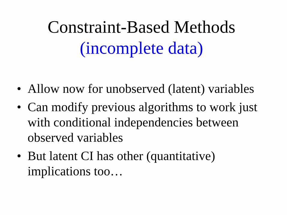
Constraint-Based Methods(incomplete data)

• Allow now for unobserved (latent) variables• Can modify previous algorithms to work just

with conditional independencies between observed variables

• But latent CI has other (quantitative) implications too…

– does not depend on a

A C

U

B D

No CI properties between observables A, B, C, D.

But

Discrete variables:

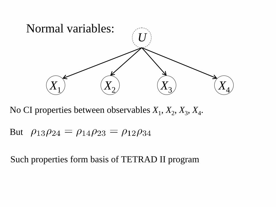
No CI properties between observables X1, X2, X3, X4.

But

Normal variables:

X2X1

U

X4X3

Such properties form basis of TETRAD II program

Bayesian Model Selection

• Consider collection M = {M} of models• Have prior distribution M(M) for parameter M

of model M• Based on data x, compute marginal likelihood for

each model M: LM = ∫ p(x | M) dM

• Use as score for comparing models, or combine with prior distribution {wM} over models to get posterior:

w*M ∝ wM LM

• Algebraically straightforward for discrete or Gaussian DAG models, parametrised by parent-child conditional distributions, having conjugate priors (with local and global independence) Zoubin Ghahramani’s lectures

• Can arrange hyperparameters so that indistinguishable (Markov equivalent) models get same score

Bayesian Model Selection

Mixed data

• Data from experimental and observational regimes

• Model-selection approach: – assume Pearlian DAG– ignore local likelihood contribution when the

response variable is set• Constraint-based approach?

– base on ECI properties, e.g.

A Parting Caution

NO CAUSES IN, NO CAUSES OUT

• We have powerful statistical methods for attacking causal problems

• But to apply them we have to make strong assumptions (e.g. ECI assumptions, relating distinct regimes)

• Important to consider and justify these in context– e.g., Mendelian randomisation

Thank you!

Further Reading• A. P. Dawid (2007). Fundamentals of Statistical Causality.

Research Report 279, Department of Statistical Science, University College London. 94 pp.http://www.ucl.ac.uk/Stats/research/reports/abs07.html#279

• R. E. Neapolitan (2003). Learning Bayesian Networks. Prentice Hall, Upper Saddle River, New Jersey.

• J. Pearl (2009). Causality: Models, Reasoning and Inference (second edition). Cambridge University Press.

• D. B. Rubin (1978). Bayesian inference for causal effects: the role of randomization. Annals of Statistics 6, 34–68.

• P. Spirtes, C. Glymour, and R. Scheines (2000). Causation, Prediction and Search (second edition). Springer-Verlag, New York.

• P. Suppes (1970). A Probabilistic Theory of Causality. North Holland, Amsterdam.