Topic Models - University of Cambridgemlg.eng.cam.ac.uk/mlss09/mlss_slides/Blei_1.pdf · Other...
81
Topic Models David M. Blei Department of Computer Science Princeton University September 1, 2009 D. Blei Topic Models
Transcript of Topic Models - University of Cambridgemlg.eng.cam.ac.uk/mlss09/mlss_slides/Blei_1.pdf · Other...

Topic Models
David M. Blei
Department of Computer SciencePrinceton University
September 1, 2009
D. Blei Topic Models

The problem with information
www.betaversion.org/~stefano/linotype/news/26/
As more information becomesavailable, it becomes more difficultto access what we are looking for.
We need new tools to help usorganize, search, and understandthese vast amounts of information.
D. Blei Topic Models

Topic modeling
Candida Hofer
Topic modeling provides methods for automatically organizing,understanding, searching, and summarizing large electronic archives.
1 Uncover the hidden topical patterns that pervade the collection.
2 Annotate the documents according to those topics.
3 Use the annotations to organize, summarize, and search the texts.
D. Blei Topic Models

Discover topics from a corpus
“Genetics” “Evolution” “Disease” “Computers”
human evolution disease computergenome evolutionary host models
dna species bacteria informationgenetic organisms diseases datagenes life resistance computers
sequence origin bacterial systemgene biology new network
molecular groups strains systemssequencing phylogenetic control model
map living infectious parallelinformation diversity malaria methods
genetics group parasite networksmapping new parasites softwareproject two united new
sequences common tuberculosis simulations
D. Blei Topic Models

Model the evolution of topics over time
1880 1900 1920 1940 1960 1980 2000
o o o o o o o ooooooooo o o o o o o o o o
o o o o oo o o
o oo o
o oooo
o
oooo
oo o
o o oo o
oooo o
o
o
ooo
o
o
o
oo o o
o o o
1880 1900 1920 1940 1960 1980 2000
o o ooo o
oooo o o o
oo o o o o o
o o o o o
o o oooo
ooooo o
o
o
oooooo o
ooo o
o o o o o o o o o oo o
o ooo
o
o
oo o o o o o
RELATIVITY
LASERFORCE
NERVE
OXYGEN
NEURON
"Theoretical Physics" "Neuroscience"
D. Blei Topic Models

Model connections between topics
wild typemutant
mutationsmutantsmutation
plantsplantgenegenes
arabidopsis
p53cell cycleactivitycyclin
regulation
amino acidscdna
sequenceisolatedprotein
genedisease
mutationsfamiliesmutation
rnadna
rna polymerasecleavage
site
cellscell
expressioncell lines
bone marrow
united stateswomen
universitiesstudents
education
sciencescientists
saysresearchpeople
researchfundingsupport
nihprogram
surfacetip
imagesampledevice
laseropticallight
electronsquantum
materialsorganicpolymerpolymersmolecules
volcanicdepositsmagmaeruption
volcanism
mantlecrust
upper mantlemeteorites
ratios
earthquakeearthquakes
faultimages
dataancientfoundimpact
million years agoafrica
climateocean
icechanges
climate change
cellsproteins
researchersproteinfound
patientsdisease
treatmentdrugsclinical
geneticpopulationpopulationsdifferencesvariation
fossil recordbirds
fossilsdinosaurs
fossil
sequencesequences
genomedna
sequencing
bacteriabacterial
hostresistanceparasite
developmentembryos
drosophilagenes
expression
speciesforestforests
populationsecosystems
synapsesltp
glutamatesynapticneurons
neuronsstimulusmotorvisual
cortical
ozoneatmospheric
measurementsstratosphere
concentrations
sunsolar wind
earthplanetsplanet
co2carbon
carbon dioxidemethane
water
receptorreceptors
ligandligands
apoptosis
proteinsproteinbindingdomaindomains
activatedtyrosine phosphorylation
activationphosphorylation
kinase
magneticmagnetic field
spinsuperconductivitysuperconducting
physicistsparticlesphysicsparticle
experimentsurfaceliquid
surfacesfluid
model reactionreactionsmoleculemolecules
transition state
enzymeenzymes
ironactive sitereduction
pressurehigh pressure
pressurescore
inner core
brainmemorysubjects
lefttask
computerproblem
informationcomputersproblems
starsastronomers
universegalaxiesgalaxy
virushiv
aidsinfectionviruses
miceantigent cells
antigensimmune response
D. Blei Topic Models

Annotate imagesAutomatic image annotation
birds nest leaves branch treepredicted caption: predicted caption:
people market pattern textile displaysky water tree mountain peoplepredicted caption:
fish water ocean tree coral sky water buildings people mountainpredicted caption: predicted caption: predicted caption:
scotland water flowers hills tree
Probabilistic modelsof text and images – p.5/53
SKY WATER TREE
MOUNTAIN PEOPLE
Automatic image annotation
birds nest leaves branch treepredicted caption: predicted caption:
people market pattern textile displaysky water tree mountain peoplepredicted caption:
fish water ocean tree coral sky water buildings people mountainpredicted caption: predicted caption: predicted caption:
scotland water flowers hills tree
Probabilistic modelsof text and images – p.5/53
SCOTLAND WATER
FLOWER HILLS TREE
Automatic image annotation
birds nest leaves branch treepredicted caption: predicted caption:
people market pattern textile displaysky water tree mountain peoplepredicted caption:
fish water ocean tree coral sky water buildings people mountainpredicted caption: predicted caption: predicted caption:
scotland water flowers hills tree
Probabilistic modelsof text and images – p.5/53
SKY WATER BUILDING
PEOPLE WATER
Automatic image annotation
birds nest leaves branch treepredicted caption: predicted caption:
people market pattern textile displaysky water tree mountain peoplepredicted caption:
fish water ocean tree coral sky water buildings people mountainpredicted caption: predicted caption: predicted caption:
scotland water flowers hills tree
Probabilistic modelsof text and images – p.5/53
FISH WATER OCEAN
TREE CORAL
Automatic image annotation
birds nest leaves branch treepredicted caption: predicted caption:
people market pattern textile displaysky water tree mountain peoplepredicted caption:
fish water ocean tree coral sky water buildings people mountainpredicted caption: predicted caption: predicted caption:
scotland water flowers hills tree
Probabilistic modelsof text and images – p.5/53
PEOPLE MARKET PATTERN
TEXTILE DISPLAY
Automatic image annotation
birds nest leaves branch treepredicted caption: predicted caption:
people market pattern textile displaysky water tree mountain peoplepredicted caption:
fish water ocean tree coral sky water buildings people mountainpredicted caption: predicted caption: predicted caption:
scotland water flowers hills tree
Probabilistic modelsof text and images – p.5/53
BIRDS NEST TREE
BRANCH LEAVES
D. Blei Topic Models

Topic modeling topics
From a machine learning perspective, topic modeling is a case study inapplying hierarchical Bayesian models to grouped data, like documents orimages. Topic modeling research touches on
• Directed graphical models
• Conjugate priors and nonconjugate priors
• Time series modeling
• Modeling with graphs
• Hierarchical Bayesian methods
• Fast approximate posterior inference (MCMC, variational methods)
• Exploratory data analysis
• Model selection and nonparametric Bayesian methods
• Mixed membership models
D. Blei Topic Models

Latent Dirichlet allocation (LDA)
1 Introduction to LDA
2 The posterior distribution for LDA
Approximate posterior inference
1 Gibbs sampling
2 Variational inference
3 Comparison/Theory/Advice
Other topic models
1 Topic models for prediction: Relational and supervised topic models
2 The logistic normal: Dynamic and correlated topic models
3 “Infinite” topic models, i.e., the hierarchical Dirichlet process
Interpreting and evaluating topic models
D. Blei Topic Models

Latent Dirichlet Allocation
D. Blei Topic Models

Probabilistic modeling
1 Treat data as observations that arise from a generative probabilisticprocess that includes hidden variables
• For documents, the hidden variables reflect the thematicstructure of the collection.
2 Infer the hidden structure using posterior inference
• What are the topics that describe this collection?
3 Situate new data into the estimated model.
• How does this query or new document fit into the estimatedtopic structure?
D. Blei Topic Models

Intuition behind LDA
Simple intuition: Documents exhibit multiple topics.
D. Blei Topic Models

Generative model
gene 0.04dna 0.02genetic 0.01.,,
life 0.02evolve 0.01organism 0.01.,,
brain 0.04neuron 0.02nerve 0.01...
data 0.02number 0.02computer 0.01.,,
Topics Documents Topic proportions andassignments
• Each document is a random mixture of corpus-wide topics
• Each word is drawn from one of those topics
D. Blei Topic Models

The posterior distribution
Topics Documents Topic proportions andassignments
• In reality, we only observe the documents
• Our goal is to infer the underlying topic structure
D. Blei Topic Models

Graphical models (Aside)
· · ·
Y
X1 X2 XN
Xn
Y
N
!
• Nodes are random variables
• Edges denote possible dependence
• Observed variables are shaded
• Plates denote replicated structure
D. Blei Topic Models

Graphical models (Aside)
· · ·
Y
X1 X2 XN
Xn
Y
N
!
• Structure of the graph defines the pattern of conditional dependencebetween the ensemble of random variables
• E.g., this graph corresponds to
p(y , x1, . . . , xN) = p(y)N∏
n=1
p(xn | y)
D. Blei Topic Models
Latent Dirichlet allocation
θd Zd,n Wd,nN
D K!k
! !
Dirichletparameter
Per-documenttopic proportions
Per-wordtopic assignment
Observedword Topics
Topichyperparameter
Each piece of the structure is a random variable.
D. Blei Topic Models

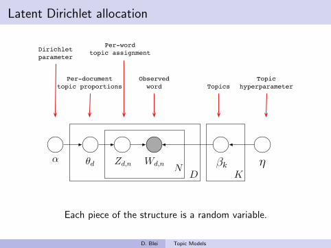
The Dirichlet distribution
• The Dirichlet distribution is an exponential family distribution overthe simplex, i.e., positive vectors that sum to one
p(θ | ~α) =Γ (∑
i αi )∏i Γ(αi )
∏
i
θαi−1i .
• The Dirichlet is conjugate to the multinomial. Given a multinomialobservation, the posterior distribution of θ is a Dirichlet.
• The parameter α controls the mean shape and sparsity of θ.
• The topic proportions are a K dimensional Dirichlet.The topics are a V dimensional Dirichlet.
D. Blei Topic Models
The Dirichlet distribution
(From Wikipedia)
D. Blei Topic Models

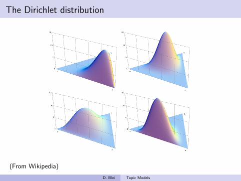
Latent Dirichlet allocation
!d Zd,n Wd,nN
D K!k
! !
• LDA is a mixed membership model (Erosheva, 2004) that builds onthe work of Deerwester et al. (1990) and Hofmann (1999).
• For document collections and other grouped data, this might bemore appropriate than a simple finite mixture.
• The same model was independently invented for population geneticsanalysis (Pritchard et al., 2000).
D. Blei Topic Models

Latent Dirichlet allocation
!d Zd,n Wd,nN
D K!k
! !
• From a collection of documents, infer
• Per-word topic assignment zd ,n
• Per-document topic proportions θd• Per-corpus topic distributions βk
• Use posterior expectations to perform the task at hand, e.g.,information retrieval, document similarity, etc.
D. Blei Topic Models

Latent Dirichlet allocation
!d Zd,n Wd,nN
D K!k
! !
Approximate posterior inference algorithms
• Mean field variational methods (Blei et al., 2001, 2003)
• Expectation propagation (Minka and Lafferty, 2002)
• Collapsed Gibbs sampling (Griffiths and Steyvers, 2002)
• Collapsed variational inference (Teh et al., 2006)
For comparison, see Mukherjee and Blei (2009) and Asuncion et al. (2009).
D. Blei Topic Models

Example inference
• Data: The OCR’ed collection of Science from 1990–2000
• 17K documents• 11M words• 20K unique terms (stop words and rare words removed)
• Model: 100-topic LDA model using variational inference.
D. Blei Topic Models

Example inference
1 8 16 26 36 46 56 66 76 86 96
Topics
Probability
0.0
0.1
0.2
0.3
0.4
D. Blei Topic Models

Example inference
“Genetics” “Evolution” “Disease” “Computers”
human evolution disease computergenome evolutionary host models
dna species bacteria informationgenetic organisms diseases datagenes life resistance computers
sequence origin bacterial systemgene biology new network
molecular groups strains systemssequencing phylogenetic control model
map living infectious parallelinformation diversity malaria methods
genetics group parasite networksmapping new parasites softwareproject two united new
sequences common tuberculosis simulations
D. Blei Topic Models

Example inference (II)
D. Blei Topic Models

Example inference (II)
problem model selection speciesproblems rate male forest
mathematical constant males ecologynumber distribution females fish
new time sex ecologicalmathematics number species conservationuniversity size female diversity
two values evolution populationfirst value populations natural
numbers average population ecosystemswork rates sexual populationstime data behavior endangered
mathematicians density evolutionary tropicalchaos measured genetic forests
chaotic models reproductive ecosystem
D. Blei Topic Models

Used to explore and browse document collections
measuredaveragerangevalues
differentsizethree
calculatedtwolow
sequenceregion
pcridentifiedfragments
twogenesthreecdna
analysis
residuesbindingdomains
helixcys
regionsstructureterminusterminal
site
computermethodsnumber
twoprincipledesignaccess
processingadvantageimportant
0.00
0.10
0.20
Top Ten Similar Documents
Exhaustive Matching of the Entire Protein Sequence DatabaseHow Big Is the Universe of Exons?Counting and Discounting the Universe of ExonsDetecting Subtle Sequence Signals: A Gibbs Sampling Strategy for Multiple AlignmentAncient Conserved Regions in New Gene Sequences and the Protein DatabasesA Method to Identify Protein Sequences that Fold into a Known Three- Dimensional StructureTesting the Exon Theory of Genes: The Evidence from Protein StructurePredicting Coiled Coils from Protein SequencesGenome Sequence of the Nematode C. elegans: A Platform for Investigating Biology
Top words from the top topics (by term score) Expected topic proportions
Abstract with the most likely topic assignments
D. Blei Topic Models

Why does LDA “work”?
Why does the LDA posterior put “topical” words together?
• Word probabilities are maximized by dividing the words among thetopics. (More terms means more mass to be spread around.)
• In a mixture, this is enough to find clusters of co-occurring words.
• In LDA, the Dirichlet on the topic proportions can encouragesparsity, i.e., a document is penalized for using many topics.
• Loosely, this can be thought of as softening the strict definition of“co-occurrence” in a mixture model.
• This flexibility leads to sets of terms that more tightly co-occur.
D. Blei Topic Models

LDA is modular, general, useful
Dynamic Topic Models
ways, and quantitative results that demonstrate greater pre-
dictive accuracy when compared with static topic models.
2. Dynamic Topic Models
While traditional time series modeling has focused on con-
tinuous data, topic models are designed for categorical
data. Our approach is to use state space models on the nat-
ural parameter space of the underlying topic multinomials,
as well as on the natural parameters for the logistic nor-
mal distributions used for modeling the document-specific
topic proportions.
First, we review the underlying statistical assumptions of
a static topic model, such as latent Dirichlet allocation
(LDA) (Blei et al., 2003). Let !1:K be K topics, each of
which is a distribution over a fixed vocabulary. In a static
topic model, each document is assumed drawn from the
following generative process:
1. Choose topic proportions " from a distribution over
the (K ! 1)-simplex, such as a Dirichlet.
2. For each word:
(a) Choose a topic assignment Z " Mult(").
(b) Choose a wordW " Mult(!z).
This process implicitly assumes that the documents are
drawn exchangeably from the same set of topics. For many
collections, however, the order of the documents reflects
an evolving set of topics. In a dynamic topic model, we
suppose that the data is divided by time slice, for example
by year. We model the documents of each slice with a K-component topic model, where the topics associated with
slice t evolve from the topics associated with slice t ! 1.
For a K-component model with V terms, let !t,k denote
the V -vector of natural parameters for topic k in slice t.The usual representation of a multinomial distribution is by
its mean parameterization. If we denote the mean param-
eter of a V -dimensional multinomial by #, the ith com-ponent of the natural parameter is given by the mapping
!i = log(#i/#V ). In typical language modeling applica-tions, Dirichlet distributions are used to model uncertainty
about the distributions over words. However, the Dirichlet
is not amenable to sequential modeling. Instead, we chain
the natural parameters of each topic !t,k in a state space
model that evolves with Gaussian noise; the simplest ver-
sion of such a model is
!t,k |!t!1,k " N (!t!1,k,$2I) . (1)
Our approach is thus to model sequences of compositional
random variables by chaining Gaussian distributions in a
dynamic model and mapping the emitted values to the sim-
plex. This is an extension of the logistic normal distribu-
A A A
!!!
zzz
!!!
! !!
w w w
N N N
K
Figure 1. Graphical representation of a dynamic topic model (for
three time slices). Each topic’s natural parameters !t,k evolve
over time, together with the mean parameters "t of the logistic
normal distribution for the topic proportions.
tion (Aitchison, 1982) to time-series simplex data (West
and Harrison, 1997).
In LDA, the document-specific topic proportions " are
drawn from a Dirichlet distribution. In the dynamic topic
model, we use a logistic normal with mean % to express
uncertainty over proportions. The sequential structure be-
tween models is again captured with a simple dynamic
model
%t |%t!1 " N (%t!1, &2I) . (2)
For simplicity, we do not model the dynamics of topic cor-
relation, as was done for static models by Blei and Lafferty
(2006).
By chaining together topics and topic proportion distribu-
tions, we have sequentially tied a collection of topic mod-
els. The generative process for slice t of a sequential corpusis thus as follows:
1. Draw topics !t |!t!1 " N (!t!1,$2I).
2. Draw %t |%t!1 " N (%t!1, &2I).
3. For each document:
(a) Draw ' " N (%t, a2I)
(b) For each word:
i. Draw Z " Mult(#(')).
ii. DrawWt,d,n " Mult(#(!t,z)).
Note that # maps the multinomial natural parameters to the
mean parameters, #(!k,t)w = exp(!k,t,w)P
w exp(!k,t,w) .
The graphical model for this generative process is shown in
Figure 1. When the horizontal arrows are removed, break-
ing the time dynamics, the graphical model reduces to a set
of independent topic models. With time dynamics, the kth
D
C
T
U
! "Nd
#
$di
%$
& '
Figure 5: Modeling community with topics
sider the conditional probability P (c, u, z|!), a word ! as-sociates three variables: community, user and topic. Ourinterpretation of the semantic meaning of P (c, u, z|!) isthe probability that word ! is generated by user u undertopic z, in community c.
Unfortunately, this conditional probability cannot be com-puted directly. To get P (c, u, z|!) ,we have:
P (c, u, z|!) =P (c, u, z, !)
!c,u,zP (c, u, z, !)(3)
Consider the denominator in Eq. 3, summing over all c,u and z makes the computation impractical in terms of ef-ficiency. In addition, as shown in [7], the summing doesn’tfactorize, which makes the manipulation of denominatordi"cult. In the following section, we will show how anapproximate approach of Gibbs sampling will provide so-lutions to such problems. A faster algorithm EnF-Gibbssampling will also be introduced.
4. SEMANTICCOMMUNITYDISCOVERY:THE ALGORITHMS
In this section, we first introduce the Gibbs samplingalgorithm. Then we address the problem of semantic com-munity discovery by adapting Gibbs sampling frameworkto our models. Finally, we combine two powerful ideas:Gibbs sampling and entropy filtering to improve e"ciencyand performance, yielding a new algorithm: EnF-Gibbssampling.
4.1 Gibbs samplingGibbs sampling is an algorithm to approximate the joint
distribution of multiple variables by drawing a sequenceof samples. As a special case of the Metropolis-Hastingsalgorithm [18], Gibbs sampling is a Markov chain MonteCarlo algorithm and usually applies when the conditionalprobability distribution of each variable can be evaluated.Rather than explicitly parameterizing the distributions forvariables, Gibbs sampling integrates out the parametersand estimates the corresponding posterior probability.
Gibbs sampling was first introduced to estimate the Topic-Word model in [7]. In Gibbs sampling, a Markov chain isformed, the transition between successive states of whichis simulated by repeatedly drawing a topic for each ob-served word from its conditional probability on all othervariables. In the Author-Topic model, the algorithm goesover all documents word by word. For each word !i, the
topic zi and the author xi responsible for this word areassigned based on the posterior probability conditioned onall other variables: P (zi, xi|!i, z!i, x!i,w!i,ad). zi andxi denote the topic and author assigned to !i, while z!i
and x!i are all other assignments of topic and author ex-cluding current instance. w!i represents other observedwords in the document set and ad is the observed authorset for this document.
A key issue in using Gibbs sampling for distributionapproximation is the evaluation of conditional posteriorprobability. In Author-Topic model, given T topics and Vwords, P (zi, xi|!i, z!i,x!i,w!i, ad) is estimated by:
P (zi = j, xi = k|!i = m, z!i,x!i,w!i,ad) ! (4)
P (!i = m|xi = k)P (xi = k|zi = j) ! (5)
CWTmj + "
!m!CWTm!j + V "
CATkj + #
!j!CATkj! + T#
(6)
where m" "= m and j" "= j, # and " are prior parametersfor word and topic Dirichlets, CWT
mj represents the numberof times that word !i = m is assigned to topic zi = j,CAT
kj represents the number of times that author xi = k isassigned to topic j.
The transformation from Eq. 4 to Eq. 5 drops the vari-ables, z!i, x!i, w!i, ad, because each instance of !i isassumed independent of the other words in a message.
4.2 Semantic community discoveryBy applying the Gibbs sampling, we can discover the se-
mantic communities by using the CUT models. Considerthe conditional probability P (c, u, z|!), where three vari-ables in the model, community, user4 and topic, are asso-ciated by a word !. The semantic meaning of P (c, u, z|!)is the probability that ! belongs to user u under topic z,in community c. By estimation of P (c, u, z|!), we can la-bel a community with semantic tags (topics) in addition tothe a"liated users. The problem of semantic communitydiscovery is thus reduced to the estimation of P (c, u, z|!).
(1) /* Initialization */(2) for each email d(3) for each word !i in d(4) assign !i to random community, topic and user;(5) /* user in the list observed from d */(6) /* Markov chain convergence */(7) i# 0;(8) I # desired number of iterations;(9) while i < I(10) for each email d(11) for each !i $ d(12) estimate P (ci, ui, zi|!i), u $ #d;(13) (p, q, r)# argmax(P (cp, uq , zr|!i));(14) /*assign community p,user q, topic r to !i*/(15) record assignment $ (cp, uq , zr, !i);(16) i + +;
Figure 6: Gibbs sampling for CUT models
4Note we denote user with u in our models instead of x asin previous work.
177
z
w
D
!
"
#
$
T dN
z
w
D
!
0"
#
$
Td
N
%
2"
x
&
'1"
(
(a) (b)
Figure 1: Graphical models for (a) the standard LDA topic model (left) and (b) the proposed specialwords topic model with a background distribution (SWB) (right).
are generated by drawing a topic t from the document-topic distribution p(z|!d) and then drawinga word w from the topic-word distribution p(w|z = t, "t). As shown in Griffiths and Steyvers(2004) the topic assignments z for each word token in the corpus can be efficiently sampled viaGibbs sampling (after marginalizing over ! and "). Point estimates for the ! and " distributionscan be computed conditioned on a particular sample, and predictive distributions can be obtained byaveraging over multiple samples.
We will refer to the proposed model as the special words topic model with background distribution(SWB) (Figure 1(b)). SWB has a similar general structure to the LDA model (Figure 1(a)) but withadditional machinery to handle special words and background words. In particular, associated witheach word token is a latent random variable x, taking value x = 0 if the word w is generated viathe topic route, value x = 1 if the word is generated as a special word (for that document) andvalue x = 2 if the word is generated from a background distribution specific for the corpus. Thevariable x acts as a switch: if x = 0, the previously described standard topic mechanism is usedto generate the word, whereas if x = 1 or x = 2, words are sampled from a document-specificmultinomial! or a corpus specific multinomial" (with symmetric Dirichlet priors parametrized by#1 and #2) respectively. x is sampled from a document-specific multinomial $, which in turn hasa symmetric Dirichlet prior, %. One could also use a hierarchical Bayesian approach to introduceanother level of uncertainty about the Dirichlet priors (e.g., see Blei, Ng, and Jordan, 2003)—wehave not investigated this option, primarily for computational reasons. In all our experiments, weset & = 0.1, #0 = #2 = 0.01, #1 = 0.0001 and % = 0.3—all weak symmetric priors.
The conditional probability of a word w given a document d can be written as:
p(w|d) = p(x = 0|d)T!
t=1
p(w|z = t)p(z = t|d) + p(x = 1|d)p!(w|d) + p(x = 2|d)p!!(w)
where p!(w|d) is the special word distribution for document d, and p!!(w) is the background worddistribution for the corpus. Note that when compared to the standard topic model the SWB modelcan explain words in three different ways, via topics, via a special word distribution, or via a back-ground word distribution. Given the graphical model above, it is relatively straightforward to deriveGibbs sampling equations that allow joint sampling of the zi and xi latent variables for each wordtoken wi, for xi = 0:
p (xi = 0, zi = t |w,x"i, z"i, &, #0, % ) ! Nd0,"i + %
Nd,"i + 3%"
CTDtd,"i + &"
t! CTDt!d,"i + T&
"CWT
wt,"i + #0"w! CWT
w!t,"i + W#0
and for xi = 1:
p (xi = 1 |w,x"i, z"i, #1, % ) ! Nd1,"i + %
Nd,"i + 3%"
CWDwd,"i + #1"
w! CWDw!d,"i + W#1
McCallum, Wang, & Corrada-Emmanuel
!
"
z
w
Latent Dirichlet Allocation
(LDA)[Blei, Ng, Jordan, 2003]
N
D
x
z
w
Author-Topic Model
(AT)[Rosen-Zvi, Griffiths, Steyvers, Smyth 2004]
N
D
"
#
!
$
T
A
#$
T
x
z
w
Author-Recipient-Topic Model
(ART)[This paper]
N
D
"
#
!
$
T
A,A
z
w
Author Model
(Multi-label Mixture Model)[McCallum 1999]
N
D
#$
A
ad ad rda
ddd
d
d
Figure 1: Three related models, and the ART model. In all models, each observed word,w, is generated from a multinomial word distribution, !z, specific to a particulartopic/author, z, however topics are selected di!erently in each of the models.In LDA, the topic is sampled from a per-document topic distribution, ", whichin turn is sampled from a Dirichlet over topics. In the Author Model, there isone topic associated with each author (or category), and authors are sampleduniformly. In the Author-Topic model, the topic is sampled from a per-authormultinomial distribution, ", and authors are sampled uniformly from the observedlist of the document’s authors. In the Author-Recipient-Topic model, there isa separate topic-distribution for each author-recipient pair, and the selection oftopic-distribution is determined from the observed author, and by uniformly sam-pling a recipient from the set of recipients for the document.
its generative process for each document d, a set of authors, ad, is observed. To generateeach word, an author x is chosen uniformly from this set, then a topic z is selected from atopic distribution "x that is specific to the author, and then a word w is generated from atopic-specific multinomial distribution !z. However, as described previously, none of thesemodels is suitable for modeling message data.
An email message has one sender and in general more than one recipients. We couldtreat both the sender and the recipients as “authors” of the message, and then employ theAT model, but this does not distinguish the author and the recipients of the message, whichis undesirable in many real-world situations. A manager may send email to a secretary andvice versa, but the nature of the requests and language used may be quite di!erent. Evenmore dramatically, consider the large quantity of junk email that we receive; modeling thetopics of these messages as undistinguished from the topics we write about as authors wouldbe extremely confounding and undesirable since they do not reflect our expertise or roles.
Alternatively we could still employ the AT model by ignoring the recipient informationof email and treating each email document as if it only has one author. However, in thiscase (which is similar to the LDA model) we are losing all information about the recipients,and the connections between people implied by the sender-recipient relationships.
252
network
neural
networks
output
...
image
images
object
objects
...
support
vector
svm
...
kernel
in
with
for
on
...
used
trained
obtained
described
...
0.5 0.4 0.1
0.7
0.9
0.8
0.2
neural network trained with svm images
image
output
network forused images
kernelwithobtained
described with objects
s s s s1 42 3
w w w w1 42 3
z z z z
!
1 42 3
(a) (b)
Figure 1: The composite model. (a) Graphical model. (b) Generating phrases.
!(z), each class c != 1 is associated with a distribution over words !(c), each document
d has a distribution over topics "(d), and transitions between classes ci!1 and ci follow a
distribution #(si!1). A document is generated via the following procedure:
1. Sample !(d) from a Dirichlet(") prior
2. For each word wi in document d
(a) Draw zi from !(d)
(b) Draw ci from #(ci!1)
(c) If ci = 1, then draw wi from $(zi), else draw wi from $(ci)
Figure 1(b) provides an intuitive representation of how phrases are generated by the com-posite model. The figure shows a three class HMM. Two classes are simple multinomialdistributions over words. The third is a topic model, containing three topics. Transitionsbetween classes are shown with arrows, annotated with transition probabilities. The top-ics in the semantic class also have probabilities, used to choose a topic when the HMMtransitions to the semantic class. Phrases are generated by following a path through themodel, choosing a word from the distribution associated with each syntactic class, and atopic followed by a word from the distribution associated with that topic for the seman-tic class. Sentences with the same syntax but different content would be generated if thetopic distribution were different. The generative model thus acts like it is playing a gameof “Madlibs”: the semantic component provides a list of topical words (shown in black)which are slotted into templates generated by the syntactic component (shown in gray).
2.2 Inference
The EM algorithm can be applied to the graphical model shown in Figure 1, treating thedocument distributions ", the topics and classes !, and the transition probabilities # asparameters. However, EM produces poor results with topic models, which have many pa-rameters and many local maxima. Consequently, recent work has focused on approximateinference algorithms [6, 8]. We will use Markov chain Monte Carlo (MCMC; see [9]) toperform full Bayesian inference in this model, sampling from a posterior distribution overassignments of words to classes and topics.
We assume that the document-specific distributions over topics, ", are drawn from a
Dirichlet($) distribution, the topic distributions !(z) are drawn from a Dirichlet(%) dis-tribution, the rows of the transition matrix for the HMM are drawn from a Dirichlet(&)distribution, the class distributions !(c) are drawn from a Dirichlet(') distribution, and allDirichlet distributions are symmetric. We use Gibbs sampling to draw iteratively a topicassignment zi and class assignment ci for each word wi in the corpus (see [8, 9]).
Given the words w, the class assignments c, the other topic assignments z!i, and thehyperparameters, each zi is drawn from:
P (zi|z!i, c,w) " P (zi|z!i) P (wi|z, c,w!i)
"!
n(di)zi + $
(n(di)zi + $)
n(zi)wi
+!
n(zi)+W!
ci != 1ci = 1
constraints of word alignment, i.e., words “close-in-source” are usually aligned to words “close-in-target”, under document-specific topical assignment. To incorporate such constituents, we integratethe strengths of both HMM and BiTAM, and propose a Hidden Markov Bilingual Topic-AdMixturemodel, or HM-BiTAM, for word alignment to leverage both locality constraints and topical contextunderlying parallel document-pairs.
In the HM-BiTAM framework, one can estimate topic-specific word-to-word translation lexicons(lexical mappings), as well as the monolingual topic-specific word-frequencies for both languages,based on parallel document-pairs. The resulting model offers a principled way of inferring optimaltranslation from a given source language in a context-dependent fashion. We report an extensiveempirical analysis of HM-BiTAM, in comparison with related methods. We show our model’s ef-fectiveness on the word-alignment task; we also demonstrate two application aspects which wereuntouched in [10]: the utility of HM-BiTAM for bilingual topic exploration, and its application forimproving translation qualities.
2 Revisit HMM for SMT
An SMT system can be formulated as a noisy-channel model [2]:
e! = arg maxe
P (e|f) = arg maxe
P (f |e)P (e), (1)
where a translation corresponds to searching for the target sentence e! which explains the sourcesentence f best. The key component is P (f |e), the translation model; P (e) is monolingual languagemodel. In this paper, we generalize P (f |e) with topic-admixture models.
An HMM implements the “proximity-bias” assumption — that words “close-in-source” are alignedto words “close-in-target”, which is effective for improving word alignment accuracies, especiallyfor linguistically close language-pairs [8]. Following [8], to model word-to-word translation, weintroduce the mapping j ! aj , which assigns a French word fj in position j to an English wordei in position i = aj denoted as eaj . Each (ordered) French word fj is an observation, and it isgenerated by an HMM state defined as [eaj
, aj], where the alignment indicator aj for position j isconsidered to have a dependency on the previous alignment aj"1. Thus a first-order HMM for analignment between e " e1:I and f " f1:J is defined as:
p(f1:J |e1:I) =!
a1:J
J"
j=1
p(fj |eaj)p(aj |aj"1), (2)
where p(aj |aj"1) is the state transition probability; J and I are sentence lengths of the French andEnglish sentences, respectively. The transition model enforces the proximity-bias. An additionalpseudo word ”NULL” is used at the beginning of English sentences for HMM to start with. TheHMM implemented in GIZA++ [5] is used as our baseline, which includes refinements such asspecial treatment of a jump to a NULL word. A graphical model representation for such an HMMis illustrated in Figure 1 (a).
Ti,i!
fm,3fm,2fm,1 fJm,n
M
am,3am,2am,1 aJm,n
em,i
Im,n
B = p(f |e)
Nm
! zm,n"m
fm,3fm,2fm,1
Bk
fJm,n
Nm
M
am,3am,2am,1
em,i
Im,n
Ti,i!
#k
K
K
aJm,n
(a) HMM for Word Alignment (b) HM-BiTAM
Figure 1: The graphical model representations of (a) HMM, and (b) HM-BiTAM, for parallel corpora. Circlesrepresent random variables, hexagons denote parameters, and observed variables are shaded.
2• LDA can be embedded in more complicated models, embodyingfurther intuitions about the structure of the texts.
• E.g., syntax; authorship; word sense; dynamics; correlation;hierarchies; nonparametric Bayes
D. Blei Topic Models

LDA is modular, general, useful
Dynamic Topic Models
ways, and quantitative results that demonstrate greater pre-
dictive accuracy when compared with static topic models.
2. Dynamic Topic Models
While traditional time series modeling has focused on con-
tinuous data, topic models are designed for categorical
data. Our approach is to use state space models on the nat-
ural parameter space of the underlying topic multinomials,
as well as on the natural parameters for the logistic nor-
mal distributions used for modeling the document-specific
topic proportions.
First, we review the underlying statistical assumptions of
a static topic model, such as latent Dirichlet allocation
(LDA) (Blei et al., 2003). Let !1:K be K topics, each of
which is a distribution over a fixed vocabulary. In a static
topic model, each document is assumed drawn from the
following generative process:
1. Choose topic proportions " from a distribution over
the (K ! 1)-simplex, such as a Dirichlet.
2. For each word:
(a) Choose a topic assignment Z " Mult(").
(b) Choose a wordW " Mult(!z).
This process implicitly assumes that the documents are
drawn exchangeably from the same set of topics. For many
collections, however, the order of the documents reflects
an evolving set of topics. In a dynamic topic model, we
suppose that the data is divided by time slice, for example
by year. We model the documents of each slice with a K-component topic model, where the topics associated with
slice t evolve from the topics associated with slice t ! 1.
For a K-component model with V terms, let !t,k denote
the V -vector of natural parameters for topic k in slice t.The usual representation of a multinomial distribution is by
its mean parameterization. If we denote the mean param-
eter of a V -dimensional multinomial by #, the ith com-ponent of the natural parameter is given by the mapping
!i = log(#i/#V ). In typical language modeling applica-tions, Dirichlet distributions are used to model uncertainty
about the distributions over words. However, the Dirichlet
is not amenable to sequential modeling. Instead, we chain
the natural parameters of each topic !t,k in a state space
model that evolves with Gaussian noise; the simplest ver-
sion of such a model is
!t,k |!t!1,k " N (!t!1,k,$2I) . (1)
Our approach is thus to model sequences of compositional
random variables by chaining Gaussian distributions in a
dynamic model and mapping the emitted values to the sim-
plex. This is an extension of the logistic normal distribu-
A A A
!!!
zzz
!!!
! !!
w w w
N N N
K
Figure 1. Graphical representation of a dynamic topic model (for
three time slices). Each topic’s natural parameters !t,k evolve
over time, together with the mean parameters "t of the logistic
normal distribution for the topic proportions.
tion (Aitchison, 1982) to time-series simplex data (West
and Harrison, 1997).
In LDA, the document-specific topic proportions " are
drawn from a Dirichlet distribution. In the dynamic topic
model, we use a logistic normal with mean % to express
uncertainty over proportions. The sequential structure be-
tween models is again captured with a simple dynamic
model
%t |%t!1 " N (%t!1, &2I) . (2)
For simplicity, we do not model the dynamics of topic cor-
relation, as was done for static models by Blei and Lafferty
(2006).
By chaining together topics and topic proportion distribu-
tions, we have sequentially tied a collection of topic mod-
els. The generative process for slice t of a sequential corpusis thus as follows:
1. Draw topics !t |!t!1 " N (!t!1,$2I).
2. Draw %t |%t!1 " N (%t!1, &2I).
3. For each document:
(a) Draw ' " N (%t, a2I)
(b) For each word:
i. Draw Z " Mult(#(')).
ii. DrawWt,d,n " Mult(#(!t,z)).
Note that # maps the multinomial natural parameters to the
mean parameters, #(!k,t)w = exp(!k,t,w)P
w exp(!k,t,w) .
The graphical model for this generative process is shown in
Figure 1. When the horizontal arrows are removed, break-
ing the time dynamics, the graphical model reduces to a set
of independent topic models. With time dynamics, the kth
D
C
T
U
! "Nd
#
$di
%$
& '
Figure 5: Modeling community with topics
sider the conditional probability P (c, u, z|!), a word ! as-sociates three variables: community, user and topic. Ourinterpretation of the semantic meaning of P (c, u, z|!) isthe probability that word ! is generated by user u undertopic z, in community c.
Unfortunately, this conditional probability cannot be com-puted directly. To get P (c, u, z|!) ,we have:
P (c, u, z|!) =P (c, u, z, !)
!c,u,zP (c, u, z, !)(3)
Consider the denominator in Eq. 3, summing over all c,u and z makes the computation impractical in terms of ef-ficiency. In addition, as shown in [7], the summing doesn’tfactorize, which makes the manipulation of denominatordi"cult. In the following section, we will show how anapproximate approach of Gibbs sampling will provide so-lutions to such problems. A faster algorithm EnF-Gibbssampling will also be introduced.
4. SEMANTICCOMMUNITYDISCOVERY:THE ALGORITHMS
In this section, we first introduce the Gibbs samplingalgorithm. Then we address the problem of semantic com-munity discovery by adapting Gibbs sampling frameworkto our models. Finally, we combine two powerful ideas:Gibbs sampling and entropy filtering to improve e"ciencyand performance, yielding a new algorithm: EnF-Gibbssampling.
4.1 Gibbs samplingGibbs sampling is an algorithm to approximate the joint
distribution of multiple variables by drawing a sequenceof samples. As a special case of the Metropolis-Hastingsalgorithm [18], Gibbs sampling is a Markov chain MonteCarlo algorithm and usually applies when the conditionalprobability distribution of each variable can be evaluated.Rather than explicitly parameterizing the distributions forvariables, Gibbs sampling integrates out the parametersand estimates the corresponding posterior probability.
Gibbs sampling was first introduced to estimate the Topic-Word model in [7]. In Gibbs sampling, a Markov chain isformed, the transition between successive states of whichis simulated by repeatedly drawing a topic for each ob-served word from its conditional probability on all othervariables. In the Author-Topic model, the algorithm goesover all documents word by word. For each word !i, the
topic zi and the author xi responsible for this word areassigned based on the posterior probability conditioned onall other variables: P (zi, xi|!i, z!i, x!i,w!i,ad). zi andxi denote the topic and author assigned to !i, while z!i
and x!i are all other assignments of topic and author ex-cluding current instance. w!i represents other observedwords in the document set and ad is the observed authorset for this document.
A key issue in using Gibbs sampling for distributionapproximation is the evaluation of conditional posteriorprobability. In Author-Topic model, given T topics and Vwords, P (zi, xi|!i, z!i,x!i,w!i, ad) is estimated by:
P (zi = j, xi = k|!i = m, z!i,x!i,w!i,ad) ! (4)
P (!i = m|xi = k)P (xi = k|zi = j) ! (5)
CWTmj + "
!m!CWTm!j + V "
CATkj + #
!j!CATkj! + T#
(6)
where m" "= m and j" "= j, # and " are prior parametersfor word and topic Dirichlets, CWT
mj represents the numberof times that word !i = m is assigned to topic zi = j,CAT
kj represents the number of times that author xi = k isassigned to topic j.
The transformation from Eq. 4 to Eq. 5 drops the vari-ables, z!i, x!i, w!i, ad, because each instance of !i isassumed independent of the other words in a message.
4.2 Semantic community discoveryBy applying the Gibbs sampling, we can discover the se-
mantic communities by using the CUT models. Considerthe conditional probability P (c, u, z|!), where three vari-ables in the model, community, user4 and topic, are asso-ciated by a word !. The semantic meaning of P (c, u, z|!)is the probability that ! belongs to user u under topic z,in community c. By estimation of P (c, u, z|!), we can la-bel a community with semantic tags (topics) in addition tothe a"liated users. The problem of semantic communitydiscovery is thus reduced to the estimation of P (c, u, z|!).
(1) /* Initialization */(2) for each email d(3) for each word !i in d(4) assign !i to random community, topic and user;(5) /* user in the list observed from d */(6) /* Markov chain convergence */(7) i# 0;(8) I # desired number of iterations;(9) while i < I(10) for each email d(11) for each !i $ d(12) estimate P (ci, ui, zi|!i), u $ #d;(13) (p, q, r)# argmax(P (cp, uq , zr|!i));(14) /*assign community p,user q, topic r to !i*/(15) record assignment $ (cp, uq , zr, !i);(16) i + +;
Figure 6: Gibbs sampling for CUT models
4Note we denote user with u in our models instead of x asin previous work.
177
z
w
D
!
"
#
$
T dN
z
w
D
!
0"
#
$
Td
N
%
2"
x
&
'1"
(
(a) (b)
Figure 1: Graphical models for (a) the standard LDA topic model (left) and (b) the proposed specialwords topic model with a background distribution (SWB) (right).
are generated by drawing a topic t from the document-topic distribution p(z|!d) and then drawinga word w from the topic-word distribution p(w|z = t, "t). As shown in Griffiths and Steyvers(2004) the topic assignments z for each word token in the corpus can be efficiently sampled viaGibbs sampling (after marginalizing over ! and "). Point estimates for the ! and " distributionscan be computed conditioned on a particular sample, and predictive distributions can be obtained byaveraging over multiple samples.
We will refer to the proposed model as the special words topic model with background distribution(SWB) (Figure 1(b)). SWB has a similar general structure to the LDA model (Figure 1(a)) but withadditional machinery to handle special words and background words. In particular, associated witheach word token is a latent random variable x, taking value x = 0 if the word w is generated viathe topic route, value x = 1 if the word is generated as a special word (for that document) andvalue x = 2 if the word is generated from a background distribution specific for the corpus. Thevariable x acts as a switch: if x = 0, the previously described standard topic mechanism is usedto generate the word, whereas if x = 1 or x = 2, words are sampled from a document-specificmultinomial! or a corpus specific multinomial" (with symmetric Dirichlet priors parametrized by#1 and #2) respectively. x is sampled from a document-specific multinomial $, which in turn hasa symmetric Dirichlet prior, %. One could also use a hierarchical Bayesian approach to introduceanother level of uncertainty about the Dirichlet priors (e.g., see Blei, Ng, and Jordan, 2003)—wehave not investigated this option, primarily for computational reasons. In all our experiments, weset & = 0.1, #0 = #2 = 0.01, #1 = 0.0001 and % = 0.3—all weak symmetric priors.
The conditional probability of a word w given a document d can be written as:
p(w|d) = p(x = 0|d)T!
t=1
p(w|z = t)p(z = t|d) + p(x = 1|d)p!(w|d) + p(x = 2|d)p!!(w)
where p!(w|d) is the special word distribution for document d, and p!!(w) is the background worddistribution for the corpus. Note that when compared to the standard topic model the SWB modelcan explain words in three different ways, via topics, via a special word distribution, or via a back-ground word distribution. Given the graphical model above, it is relatively straightforward to deriveGibbs sampling equations that allow joint sampling of the zi and xi latent variables for each wordtoken wi, for xi = 0:
p (xi = 0, zi = t |w,x"i, z"i, &, #0, % ) ! Nd0,"i + %
Nd,"i + 3%"
CTDtd,"i + &"
t! CTDt!d,"i + T&
"CWT
wt,"i + #0"w! CWT
w!t,"i + W#0
and for xi = 1:
p (xi = 1 |w,x"i, z"i, #1, % ) ! Nd1,"i + %
Nd,"i + 3%"
CWDwd,"i + #1"
w! CWDw!d,"i + W#1
McCallum, Wang, & Corrada-Emmanuel
!
"
z
w
Latent Dirichlet Allocation
(LDA)[Blei, Ng, Jordan, 2003]
N
D
x
z
w
Author-Topic Model
(AT)[Rosen-Zvi, Griffiths, Steyvers, Smyth 2004]
N
D
"
#
!
$
T
A
#$
T
x
z
w
Author-Recipient-Topic Model
(ART)[This paper]
N
D
"
#
!
$
T
A,A
z
w
Author Model
(Multi-label Mixture Model)[McCallum 1999]
N
D
#$
A
ad ad rda
ddd
d
d
Figure 1: Three related models, and the ART model. In all models, each observed word,w, is generated from a multinomial word distribution, !z, specific to a particulartopic/author, z, however topics are selected di!erently in each of the models.In LDA, the topic is sampled from a per-document topic distribution, ", whichin turn is sampled from a Dirichlet over topics. In the Author Model, there isone topic associated with each author (or category), and authors are sampleduniformly. In the Author-Topic model, the topic is sampled from a per-authormultinomial distribution, ", and authors are sampled uniformly from the observedlist of the document’s authors. In the Author-Recipient-Topic model, there isa separate topic-distribution for each author-recipient pair, and the selection oftopic-distribution is determined from the observed author, and by uniformly sam-pling a recipient from the set of recipients for the document.
its generative process for each document d, a set of authors, ad, is observed. To generateeach word, an author x is chosen uniformly from this set, then a topic z is selected from atopic distribution "x that is specific to the author, and then a word w is generated from atopic-specific multinomial distribution !z. However, as described previously, none of thesemodels is suitable for modeling message data.
An email message has one sender and in general more than one recipients. We couldtreat both the sender and the recipients as “authors” of the message, and then employ theAT model, but this does not distinguish the author and the recipients of the message, whichis undesirable in many real-world situations. A manager may send email to a secretary andvice versa, but the nature of the requests and language used may be quite di!erent. Evenmore dramatically, consider the large quantity of junk email that we receive; modeling thetopics of these messages as undistinguished from the topics we write about as authors wouldbe extremely confounding and undesirable since they do not reflect our expertise or roles.
Alternatively we could still employ the AT model by ignoring the recipient informationof email and treating each email document as if it only has one author. However, in thiscase (which is similar to the LDA model) we are losing all information about the recipients,and the connections between people implied by the sender-recipient relationships.
252
network
neural
networks
output
...
image
images
object
objects
...
support
vector
svm
...
kernel
in
with
for
on
...
used
trained
obtained
described
...
0.5 0.4 0.1
0.7
0.9
0.8
0.2
neural network trained with svm images
image
output
network forused images
kernelwithobtained
described with objects
s s s s1 42 3
w w w w1 42 3
z z z z
!
1 42 3
(a) (b)
Figure 1: The composite model. (a) Graphical model. (b) Generating phrases.
!(z), each class c != 1 is associated with a distribution over words !(c), each document
d has a distribution over topics "(d), and transitions between classes ci!1 and ci follow a
distribution #(si!1). A document is generated via the following procedure:
1. Sample !(d) from a Dirichlet(") prior
2. For each word wi in document d
(a) Draw zi from !(d)
(b) Draw ci from #(ci!1)
(c) If ci = 1, then draw wi from $(zi), else draw wi from $(ci)
Figure 1(b) provides an intuitive representation of how phrases are generated by the com-posite model. The figure shows a three class HMM. Two classes are simple multinomialdistributions over words. The third is a topic model, containing three topics. Transitionsbetween classes are shown with arrows, annotated with transition probabilities. The top-ics in the semantic class also have probabilities, used to choose a topic when the HMMtransitions to the semantic class. Phrases are generated by following a path through themodel, choosing a word from the distribution associated with each syntactic class, and atopic followed by a word from the distribution associated with that topic for the seman-tic class. Sentences with the same syntax but different content would be generated if thetopic distribution were different. The generative model thus acts like it is playing a gameof “Madlibs”: the semantic component provides a list of topical words (shown in black)which are slotted into templates generated by the syntactic component (shown in gray).
2.2 Inference
The EM algorithm can be applied to the graphical model shown in Figure 1, treating thedocument distributions ", the topics and classes !, and the transition probabilities # asparameters. However, EM produces poor results with topic models, which have many pa-rameters and many local maxima. Consequently, recent work has focused on approximateinference algorithms [6, 8]. We will use Markov chain Monte Carlo (MCMC; see [9]) toperform full Bayesian inference in this model, sampling from a posterior distribution overassignments of words to classes and topics.
We assume that the document-specific distributions over topics, ", are drawn from a
Dirichlet($) distribution, the topic distributions !(z) are drawn from a Dirichlet(%) dis-tribution, the rows of the transition matrix for the HMM are drawn from a Dirichlet(&)distribution, the class distributions !(c) are drawn from a Dirichlet(') distribution, and allDirichlet distributions are symmetric. We use Gibbs sampling to draw iteratively a topicassignment zi and class assignment ci for each word wi in the corpus (see [8, 9]).
Given the words w, the class assignments c, the other topic assignments z!i, and thehyperparameters, each zi is drawn from:
P (zi|z!i, c,w) " P (zi|z!i) P (wi|z, c,w!i)
"!
n(di)zi + $
(n(di)zi + $)
n(zi)wi
+!
n(zi)+W!
ci != 1ci = 1
constraints of word alignment, i.e., words “close-in-source” are usually aligned to words “close-in-target”, under document-specific topical assignment. To incorporate such constituents, we integratethe strengths of both HMM and BiTAM, and propose a Hidden Markov Bilingual Topic-AdMixturemodel, or HM-BiTAM, for word alignment to leverage both locality constraints and topical contextunderlying parallel document-pairs.
In the HM-BiTAM framework, one can estimate topic-specific word-to-word translation lexicons(lexical mappings), as well as the monolingual topic-specific word-frequencies for both languages,based on parallel document-pairs. The resulting model offers a principled way of inferring optimaltranslation from a given source language in a context-dependent fashion. We report an extensiveempirical analysis of HM-BiTAM, in comparison with related methods. We show our model’s ef-fectiveness on the word-alignment task; we also demonstrate two application aspects which wereuntouched in [10]: the utility of HM-BiTAM for bilingual topic exploration, and its application forimproving translation qualities.
2 Revisit HMM for SMT
An SMT system can be formulated as a noisy-channel model [2]:
e! = arg maxe
P (e|f) = arg maxe
P (f |e)P (e), (1)
where a translation corresponds to searching for the target sentence e! which explains the sourcesentence f best. The key component is P (f |e), the translation model; P (e) is monolingual languagemodel. In this paper, we generalize P (f |e) with topic-admixture models.
An HMM implements the “proximity-bias” assumption — that words “close-in-source” are alignedto words “close-in-target”, which is effective for improving word alignment accuracies, especiallyfor linguistically close language-pairs [8]. Following [8], to model word-to-word translation, weintroduce the mapping j ! aj , which assigns a French word fj in position j to an English wordei in position i = aj denoted as eaj . Each (ordered) French word fj is an observation, and it isgenerated by an HMM state defined as [eaj
, aj], where the alignment indicator aj for position j isconsidered to have a dependency on the previous alignment aj"1. Thus a first-order HMM for analignment between e " e1:I and f " f1:J is defined as:
p(f1:J |e1:I) =!
a1:J
J"
j=1
p(fj |eaj)p(aj |aj"1), (2)
where p(aj |aj"1) is the state transition probability; J and I are sentence lengths of the French andEnglish sentences, respectively. The transition model enforces the proximity-bias. An additionalpseudo word ”NULL” is used at the beginning of English sentences for HMM to start with. TheHMM implemented in GIZA++ [5] is used as our baseline, which includes refinements such asspecial treatment of a jump to a NULL word. A graphical model representation for such an HMMis illustrated in Figure 1 (a).
Ti,i!
fm,3fm,2fm,1 fJm,n
M
am,3am,2am,1 aJm,n
em,i
Im,n
B = p(f |e)
Nm
! zm,n"m
fm,3fm,2fm,1
Bk
fJm,n
Nm
M
am,3am,2am,1
em,i
Im,n
Ti,i!
#k
K
K
aJm,n
(a) HMM for Word Alignment (b) HM-BiTAM
Figure 1: The graphical model representations of (a) HMM, and (b) HM-BiTAM, for parallel corpora. Circlesrepresent random variables, hexagons denote parameters, and observed variables are shaded.
2• The data generating distribution can be changed.
• E.g., images, social networks, music, purchase histories, computercode, genetic data, click-through data; ...
D. Blei Topic Models

LDA is modular, general, useful
Dynamic Topic Models
ways, and quantitative results that demonstrate greater pre-
dictive accuracy when compared with static topic models.
2. Dynamic Topic Models
While traditional time series modeling has focused on con-
tinuous data, topic models are designed for categorical
data. Our approach is to use state space models on the nat-
ural parameter space of the underlying topic multinomials,
as well as on the natural parameters for the logistic nor-
mal distributions used for modeling the document-specific
topic proportions.
First, we review the underlying statistical assumptions of
a static topic model, such as latent Dirichlet allocation
(LDA) (Blei et al., 2003). Let !1:K be K topics, each of
which is a distribution over a fixed vocabulary. In a static
topic model, each document is assumed drawn from the
following generative process:
1. Choose topic proportions " from a distribution over
the (K ! 1)-simplex, such as a Dirichlet.
2. For each word:
(a) Choose a topic assignment Z " Mult(").
(b) Choose a wordW " Mult(!z).
This process implicitly assumes that the documents are
drawn exchangeably from the same set of topics. For many
collections, however, the order of the documents reflects
an evolving set of topics. In a dynamic topic model, we
suppose that the data is divided by time slice, for example
by year. We model the documents of each slice with a K-component topic model, where the topics associated with
slice t evolve from the topics associated with slice t ! 1.
For a K-component model with V terms, let !t,k denote
the V -vector of natural parameters for topic k in slice t.The usual representation of a multinomial distribution is by
its mean parameterization. If we denote the mean param-
eter of a V -dimensional multinomial by #, the ith com-ponent of the natural parameter is given by the mapping
!i = log(#i/#V ). In typical language modeling applica-tions, Dirichlet distributions are used to model uncertainty
about the distributions over words. However, the Dirichlet
is not amenable to sequential modeling. Instead, we chain
the natural parameters of each topic !t,k in a state space
model that evolves with Gaussian noise; the simplest ver-
sion of such a model is
!t,k |!t!1,k " N (!t!1,k,$2I) . (1)
Our approach is thus to model sequences of compositional
random variables by chaining Gaussian distributions in a
dynamic model and mapping the emitted values to the sim-
plex. This is an extension of the logistic normal distribu-
A A A
!!!
zzz
!!!
! !!
w w w
N N N
K
Figure 1. Graphical representation of a dynamic topic model (for
three time slices). Each topic’s natural parameters !t,k evolve
over time, together with the mean parameters "t of the logistic
normal distribution for the topic proportions.
tion (Aitchison, 1982) to time-series simplex data (West
and Harrison, 1997).
In LDA, the document-specific topic proportions " are
drawn from a Dirichlet distribution. In the dynamic topic
model, we use a logistic normal with mean % to express
uncertainty over proportions. The sequential structure be-
tween models is again captured with a simple dynamic
model
%t |%t!1 " N (%t!1, &2I) . (2)
For simplicity, we do not model the dynamics of topic cor-
relation, as was done for static models by Blei and Lafferty
(2006).
By chaining together topics and topic proportion distribu-
tions, we have sequentially tied a collection of topic mod-
els. The generative process for slice t of a sequential corpusis thus as follows:
1. Draw topics !t |!t!1 " N (!t!1,$2I).
2. Draw %t |%t!1 " N (%t!1, &2I).
3. For each document:
(a) Draw ' " N (%t, a2I)
(b) For each word:
i. Draw Z " Mult(#(')).
ii. DrawWt,d,n " Mult(#(!t,z)).
Note that # maps the multinomial natural parameters to the
mean parameters, #(!k,t)w = exp(!k,t,w)P
w exp(!k,t,w) .
The graphical model for this generative process is shown in
Figure 1. When the horizontal arrows are removed, break-
ing the time dynamics, the graphical model reduces to a set
of independent topic models. With time dynamics, the kth
D
C
T
U
! "Nd
#
$di
%$
& '
Figure 5: Modeling community with topics
sider the conditional probability P (c, u, z|!), a word ! as-sociates three variables: community, user and topic. Ourinterpretation of the semantic meaning of P (c, u, z|!) isthe probability that word ! is generated by user u undertopic z, in community c.
Unfortunately, this conditional probability cannot be com-puted directly. To get P (c, u, z|!) ,we have:
P (c, u, z|!) =P (c, u, z, !)
!c,u,zP (c, u, z, !)(3)
Consider the denominator in Eq. 3, summing over all c,u and z makes the computation impractical in terms of ef-ficiency. In addition, as shown in [7], the summing doesn’tfactorize, which makes the manipulation of denominatordi"cult. In the following section, we will show how anapproximate approach of Gibbs sampling will provide so-lutions to such problems. A faster algorithm EnF-Gibbssampling will also be introduced.
4. SEMANTICCOMMUNITYDISCOVERY:THE ALGORITHMS
In this section, we first introduce the Gibbs samplingalgorithm. Then we address the problem of semantic com-munity discovery by adapting Gibbs sampling frameworkto our models. Finally, we combine two powerful ideas:Gibbs sampling and entropy filtering to improve e"ciencyand performance, yielding a new algorithm: EnF-Gibbssampling.
4.1 Gibbs samplingGibbs sampling is an algorithm to approximate the joint
distribution of multiple variables by drawing a sequenceof samples. As a special case of the Metropolis-Hastingsalgorithm [18], Gibbs sampling is a Markov chain MonteCarlo algorithm and usually applies when the conditionalprobability distribution of each variable can be evaluated.Rather than explicitly parameterizing the distributions forvariables, Gibbs sampling integrates out the parametersand estimates the corresponding posterior probability.
Gibbs sampling was first introduced to estimate the Topic-Word model in [7]. In Gibbs sampling, a Markov chain isformed, the transition between successive states of whichis simulated by repeatedly drawing a topic for each ob-served word from its conditional probability on all othervariables. In the Author-Topic model, the algorithm goesover all documents word by word. For each word !i, the
topic zi and the author xi responsible for this word areassigned based on the posterior probability conditioned onall other variables: P (zi, xi|!i, z!i, x!i,w!i,ad). zi andxi denote the topic and author assigned to !i, while z!i
and x!i are all other assignments of topic and author ex-cluding current instance. w!i represents other observedwords in the document set and ad is the observed authorset for this document.
A key issue in using Gibbs sampling for distributionapproximation is the evaluation of conditional posteriorprobability. In Author-Topic model, given T topics and Vwords, P (zi, xi|!i, z!i,x!i,w!i, ad) is estimated by:
P (zi = j, xi = k|!i = m, z!i,x!i,w!i,ad) ! (4)
P (!i = m|xi = k)P (xi = k|zi = j) ! (5)
CWTmj + "
!m!CWTm!j + V "
CATkj + #
!j!CATkj! + T#
(6)
where m" "= m and j" "= j, # and " are prior parametersfor word and topic Dirichlets, CWT
mj represents the numberof times that word !i = m is assigned to topic zi = j,CAT
kj represents the number of times that author xi = k isassigned to topic j.
The transformation from Eq. 4 to Eq. 5 drops the vari-ables, z!i, x!i, w!i, ad, because each instance of !i isassumed independent of the other words in a message.
4.2 Semantic community discoveryBy applying the Gibbs sampling, we can discover the se-
mantic communities by using the CUT models. Considerthe conditional probability P (c, u, z|!), where three vari-ables in the model, community, user4 and topic, are asso-ciated by a word !. The semantic meaning of P (c, u, z|!)is the probability that ! belongs to user u under topic z,in community c. By estimation of P (c, u, z|!), we can la-bel a community with semantic tags (topics) in addition tothe a"liated users. The problem of semantic communitydiscovery is thus reduced to the estimation of P (c, u, z|!).
(1) /* Initialization */(2) for each email d(3) for each word !i in d(4) assign !i to random community, topic and user;(5) /* user in the list observed from d */(6) /* Markov chain convergence */(7) i# 0;(8) I # desired number of iterations;(9) while i < I(10) for each email d(11) for each !i $ d(12) estimate P (ci, ui, zi|!i), u $ #d;(13) (p, q, r)# argmax(P (cp, uq , zr|!i));(14) /*assign community p,user q, topic r to !i*/(15) record assignment $ (cp, uq , zr, !i);(16) i + +;
Figure 6: Gibbs sampling for CUT models
4Note we denote user with u in our models instead of x asin previous work.
177
z
w
D
!
"
#
$
T dN
z
w
D
!
0"
#
$
Td
N
%
2"
x
&
'1"
(
(a) (b)
Figure 1: Graphical models for (a) the standard LDA topic model (left) and (b) the proposed specialwords topic model with a background distribution (SWB) (right).
are generated by drawing a topic t from the document-topic distribution p(z|!d) and then drawinga word w from the topic-word distribution p(w|z = t, "t). As shown in Griffiths and Steyvers(2004) the topic assignments z for each word token in the corpus can be efficiently sampled viaGibbs sampling (after marginalizing over ! and "). Point estimates for the ! and " distributionscan be computed conditioned on a particular sample, and predictive distributions can be obtained byaveraging over multiple samples.
We will refer to the proposed model as the special words topic model with background distribution(SWB) (Figure 1(b)). SWB has a similar general structure to the LDA model (Figure 1(a)) but withadditional machinery to handle special words and background words. In particular, associated witheach word token is a latent random variable x, taking value x = 0 if the word w is generated viathe topic route, value x = 1 if the word is generated as a special word (for that document) andvalue x = 2 if the word is generated from a background distribution specific for the corpus. Thevariable x acts as a switch: if x = 0, the previously described standard topic mechanism is usedto generate the word, whereas if x = 1 or x = 2, words are sampled from a document-specificmultinomial! or a corpus specific multinomial" (with symmetric Dirichlet priors parametrized by#1 and #2) respectively. x is sampled from a document-specific multinomial $, which in turn hasa symmetric Dirichlet prior, %. One could also use a hierarchical Bayesian approach to introduceanother level of uncertainty about the Dirichlet priors (e.g., see Blei, Ng, and Jordan, 2003)—wehave not investigated this option, primarily for computational reasons. In all our experiments, weset & = 0.1, #0 = #2 = 0.01, #1 = 0.0001 and % = 0.3—all weak symmetric priors.
The conditional probability of a word w given a document d can be written as:
p(w|d) = p(x = 0|d)T!
t=1
p(w|z = t)p(z = t|d) + p(x = 1|d)p!(w|d) + p(x = 2|d)p!!(w)
where p!(w|d) is the special word distribution for document d, and p!!(w) is the background worddistribution for the corpus. Note that when compared to the standard topic model the SWB modelcan explain words in three different ways, via topics, via a special word distribution, or via a back-ground word distribution. Given the graphical model above, it is relatively straightforward to deriveGibbs sampling equations that allow joint sampling of the zi and xi latent variables for each wordtoken wi, for xi = 0:
p (xi = 0, zi = t |w,x"i, z"i, &, #0, % ) ! Nd0,"i + %
Nd,"i + 3%"
CTDtd,"i + &"
t! CTDt!d,"i + T&
"CWT
wt,"i + #0"w! CWT
w!t,"i + W#0
and for xi = 1:
p (xi = 1 |w,x"i, z"i, #1, % ) ! Nd1,"i + %
Nd,"i + 3%"
CWDwd,"i + #1"
w! CWDw!d,"i + W#1
McCallum, Wang, & Corrada-Emmanuel
!
"
z
w
Latent Dirichlet Allocation
(LDA)[Blei, Ng, Jordan, 2003]
N
D
x
z
w
Author-Topic Model
(AT)[Rosen-Zvi, Griffiths, Steyvers, Smyth 2004]
N
D
"
#
!
$
T
A
#$
T
x
z
w
Author-Recipient-Topic Model
(ART)[This paper]
N
D
"
#
!
$
T
A,A
z
w
Author Model
(Multi-label Mixture Model)[McCallum 1999]
N
D
#$
A
ad ad rda
ddd
d
d
Figure 1: Three related models, and the ART model. In all models, each observed word,w, is generated from a multinomial word distribution, !z, specific to a particulartopic/author, z, however topics are selected di!erently in each of the models.In LDA, the topic is sampled from a per-document topic distribution, ", whichin turn is sampled from a Dirichlet over topics. In the Author Model, there isone topic associated with each author (or category), and authors are sampleduniformly. In the Author-Topic model, the topic is sampled from a per-authormultinomial distribution, ", and authors are sampled uniformly from the observedlist of the document’s authors. In the Author-Recipient-Topic model, there isa separate topic-distribution for each author-recipient pair, and the selection oftopic-distribution is determined from the observed author, and by uniformly sam-pling a recipient from the set of recipients for the document.
its generative process for each document d, a set of authors, ad, is observed. To generateeach word, an author x is chosen uniformly from this set, then a topic z is selected from atopic distribution "x that is specific to the author, and then a word w is generated from atopic-specific multinomial distribution !z. However, as described previously, none of thesemodels is suitable for modeling message data.
An email message has one sender and in general more than one recipients. We couldtreat both the sender and the recipients as “authors” of the message, and then employ theAT model, but this does not distinguish the author and the recipients of the message, whichis undesirable in many real-world situations. A manager may send email to a secretary andvice versa, but the nature of the requests and language used may be quite di!erent. Evenmore dramatically, consider the large quantity of junk email that we receive; modeling thetopics of these messages as undistinguished from the topics we write about as authors wouldbe extremely confounding and undesirable since they do not reflect our expertise or roles.
Alternatively we could still employ the AT model by ignoring the recipient informationof email and treating each email document as if it only has one author. However, in thiscase (which is similar to the LDA model) we are losing all information about the recipients,and the connections between people implied by the sender-recipient relationships.
252
network
neural
networks
output
...
image
images
object
objects
...
support
vector
svm
...
kernel
in
with
for
on
...
used
trained
obtained
described
...
0.5 0.4 0.1
0.7
0.9
0.8
0.2
neural network trained with svm images
image
output
network forused images
kernelwithobtained
described with objects
s s s s1 42 3
w w w w1 42 3
z z z z
!
1 42 3
(a) (b)
Figure 1: The composite model. (a) Graphical model. (b) Generating phrases.
!(z), each class c != 1 is associated with a distribution over words !(c), each document
d has a distribution over topics "(d), and transitions between classes ci!1 and ci follow a
distribution #(si!1). A document is generated via the following procedure:
1. Sample !(d) from a Dirichlet(") prior
2. For each word wi in document d
(a) Draw zi from !(d)
(b) Draw ci from #(ci!1)
(c) If ci = 1, then draw wi from $(zi), else draw wi from $(ci)
Figure 1(b) provides an intuitive representation of how phrases are generated by the com-posite model. The figure shows a three class HMM. Two classes are simple multinomialdistributions over words. The third is a topic model, containing three topics. Transitionsbetween classes are shown with arrows, annotated with transition probabilities. The top-ics in the semantic class also have probabilities, used to choose a topic when the HMMtransitions to the semantic class. Phrases are generated by following a path through themodel, choosing a word from the distribution associated with each syntactic class, and atopic followed by a word from the distribution associated with that topic for the seman-tic class. Sentences with the same syntax but different content would be generated if thetopic distribution were different. The generative model thus acts like it is playing a gameof “Madlibs”: the semantic component provides a list of topical words (shown in black)which are slotted into templates generated by the syntactic component (shown in gray).
2.2 Inference
The EM algorithm can be applied to the graphical model shown in Figure 1, treating thedocument distributions ", the topics and classes !, and the transition probabilities # asparameters. However, EM produces poor results with topic models, which have many pa-rameters and many local maxima. Consequently, recent work has focused on approximateinference algorithms [6, 8]. We will use Markov chain Monte Carlo (MCMC; see [9]) toperform full Bayesian inference in this model, sampling from a posterior distribution overassignments of words to classes and topics.
We assume that the document-specific distributions over topics, ", are drawn from a
Dirichlet($) distribution, the topic distributions !(z) are drawn from a Dirichlet(%) dis-tribution, the rows of the transition matrix for the HMM are drawn from a Dirichlet(&)distribution, the class distributions !(c) are drawn from a Dirichlet(') distribution, and allDirichlet distributions are symmetric. We use Gibbs sampling to draw iteratively a topicassignment zi and class assignment ci for each word wi in the corpus (see [8, 9]).
Given the words w, the class assignments c, the other topic assignments z!i, and thehyperparameters, each zi is drawn from:
P (zi|z!i, c,w) " P (zi|z!i) P (wi|z, c,w!i)
"!
n(di)zi + $
(n(di)zi + $)
n(zi)wi
+!
n(zi)+W!
ci != 1ci = 1
constraints of word alignment, i.e., words “close-in-source” are usually aligned to words “close-in-target”, under document-specific topical assignment. To incorporate such constituents, we integratethe strengths of both HMM and BiTAM, and propose a Hidden Markov Bilingual Topic-AdMixturemodel, or HM-BiTAM, for word alignment to leverage both locality constraints and topical contextunderlying parallel document-pairs.
In the HM-BiTAM framework, one can estimate topic-specific word-to-word translation lexicons(lexical mappings), as well as the monolingual topic-specific word-frequencies for both languages,based on parallel document-pairs. The resulting model offers a principled way of inferring optimaltranslation from a given source language in a context-dependent fashion. We report an extensiveempirical analysis of HM-BiTAM, in comparison with related methods. We show our model’s ef-fectiveness on the word-alignment task; we also demonstrate two application aspects which wereuntouched in [10]: the utility of HM-BiTAM for bilingual topic exploration, and its application forimproving translation qualities.
2 Revisit HMM for SMT
An SMT system can be formulated as a noisy-channel model [2]:
e! = arg maxe
P (e|f) = arg maxe
P (f |e)P (e), (1)
where a translation corresponds to searching for the target sentence e! which explains the sourcesentence f best. The key component is P (f |e), the translation model; P (e) is monolingual languagemodel. In this paper, we generalize P (f |e) with topic-admixture models.
An HMM implements the “proximity-bias” assumption — that words “close-in-source” are alignedto words “close-in-target”, which is effective for improving word alignment accuracies, especiallyfor linguistically close language-pairs [8]. Following [8], to model word-to-word translation, weintroduce the mapping j ! aj , which assigns a French word fj in position j to an English wordei in position i = aj denoted as eaj . Each (ordered) French word fj is an observation, and it isgenerated by an HMM state defined as [eaj
, aj], where the alignment indicator aj for position j isconsidered to have a dependency on the previous alignment aj"1. Thus a first-order HMM for analignment between e " e1:I and f " f1:J is defined as:
p(f1:J |e1:I) =!
a1:J
J"
j=1
p(fj |eaj)p(aj |aj"1), (2)
where p(aj |aj"1) is the state transition probability; J and I are sentence lengths of the French andEnglish sentences, respectively. The transition model enforces the proximity-bias. An additionalpseudo word ”NULL” is used at the beginning of English sentences for HMM to start with. TheHMM implemented in GIZA++ [5] is used as our baseline, which includes refinements such asspecial treatment of a jump to a NULL word. A graphical model representation for such an HMMis illustrated in Figure 1 (a).
Ti,i!
fm,3fm,2fm,1 fJm,n
M
am,3am,2am,1 aJm,n
em,i
Im,n
B = p(f |e)
Nm
! zm,n"m
fm,3fm,2fm,1
Bk
fJm,n
Nm
M
am,3am,2am,1
em,i
Im,n
Ti,i!
#k
K
K
aJm,n
(a) HMM for Word Alignment (b) HM-BiTAM
Figure 1: The graphical model representations of (a) HMM, and (b) HM-BiTAM, for parallel corpora. Circlesrepresent random variables, hexagons denote parameters, and observed variables are shaded.
2• The posterior can be used in creative ways
• E.g., IR, collaborative filtering, document similarity,visualizing interdisciplinary documents
D. Blei Topic Models

Approximate posterior inference
D. Blei Topic Models

Posterior distribution for LDA
• For now, assume the topics β1:K are fixed.The per-document posterior is
p(θ |α)∏N
n=1 p(zn | θ)p(wn | zn, β1:K )∫θ p(θ |α)
∏Nn=1
∑Kz=1 p(zn | θ)p(wn | zn, β1:K )
• This is intractable to compute
• It is a “multiple hypergeometric function” (see Dickey, 1983)
• Can be seen as sum of NK (tractable) Dirichlet integral terms
D. Blei Topic Models
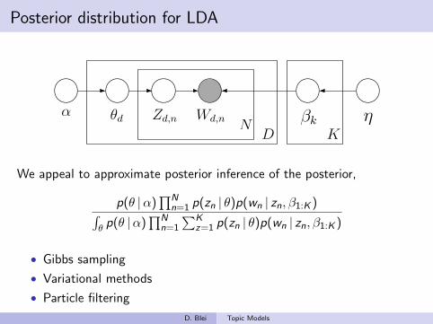
Posterior distribution for LDA
!d Zd,n Wd,nN
D K!k
! !
We appeal to approximate posterior inference of the posterior,
p(θ |α)∏N
n=1 p(zn | θ)p(wn | zn, β1:K )∫θ p(θ |α)
∏Nn=1
∑Kz=1 p(zn | θ)p(wn | zn, β1:K )
• Gibbs sampling
• Variational methods
• Particle filtering
D. Blei Topic Models

Gibbs sampling
• Define a Markov chain whose stationary distribution is theposterior of interest
• Collect independent samples from that stationary distribution;approximate the posterior with them
• In Gibbs sampling, the space of the MC is the space of possibleconfigurations of the hidden variables.
• The chain is run by iteratively sampling from the conditionaldistribution of each hidden variable given observations and thecurrent state of the other hidden variables
• Once a chain has “burned in,” collect samples at a lag toapproximate the posterior.
D. Blei Topic Models

Gibbs sampling for LDA
!d Zd,n Wd,nN
D K!k
! !
Define n(z1:N) to be the counts vector. A simple Gibbs sampler is
θ |w1:N , z1:N ∼ Dir(α + n(z1:N))
zi | z−i ,w1:N ∼ Mult(π(z−i ,wi ))
whereπ(z−i ,wi ) ∝ (α + n(z1:N))p(wi |β1:K )
D. Blei Topic Models

Gibbs sampling for LDA
!d Zd,n Wd,nN
D K!k
! !
• The topic proportions θ can be integrated out.
• A collapsed Gibbs sampler draws from
p(zi | z−i ,w1:N) ∝ p(wi |β1:K )∏K
k=1 Γ(nk(z−i )),
where nk(z−i ) is the number of times we’ve seen topic k in thecollection of topic assignments z−i .
• Integrating out variables leads to a faster mixing chain.
D. Blei Topic Models
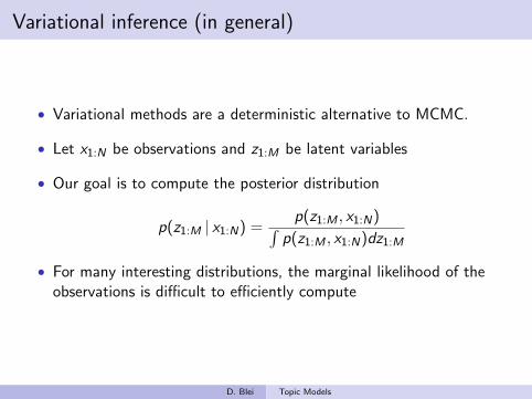
Variational inference (in general)
• Variational methods are a deterministic alternative to MCMC.
• Let x1:N be observations and z1:M be latent variables
• Our goal is to compute the posterior distribution
p(z1:M | x1:N) =p(z1:M , x1:N)∫
p(z1:M , x1:N)dz1:M
• For many interesting distributions, the marginal likelihood of theobservations is difficult to efficiently compute
D. Blei Topic Models

Variational inference
• Use Jensen’s inequality to bound the log prob of the observations:
log p(x1:N) = log
∫p(z1:M , x1:N)dz1:M
= log
∫p(z1:M , x1:N)
qν(z1:M)
qν(z1:M)dz1:M
≥ Eqν [log p(z1:M , x1:N)]− Eqν [log qν(z1:M)]
• We have introduced a distribution of the latent variables with freevariational parameters ν.
• We optimize those parameters to tighten this bound.
• This is the same as finding the member of the family qν that isclosest in KL divergence to p(z1:M | x1:N).
D. Blei Topic Models

Mean-field variational inference
• Complexity of optimization is determined by the factorization of qν
• In mean field variational inference we choose qν to be fully factored
qν(z1:M) =M∏
m=1
qνm(zm).
• The latent variables are independent.
• Each is governed by its own variational parameter νm.
• In the true posterior they can exhibit dependence(often, this is what makes exact inference difficult).
D. Blei Topic Models

MFVI and conditional exponential families
• Suppose the distribution of each latent variable conditional on theobservations and other latent variables is in the exponential family:
p(zm | z−m, x) = hm(zm) exp{gm(z−m, x)T zm − am(gi (z−m, x))}
• Assume qν is fully factorized, and each factor is in the sameexponential family:
qνm(zm) = hm(zm) exp{νTmzm − am(νm)}
D. Blei Topic Models

MFVI and conditional exponential families
• Variational inference is the following coordinate ascent algorithm
νm = Eqν [gm(Z−m, x)]
• Notice the relationship to Gibbs sampling.
• (You will hear much more about this from Minka and Winn.)
D. Blei Topic Models
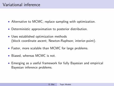
Variational inference
• Alternative to MCMC; replace sampling with optimization.
• Deterministic approximation to posterior distribution.
• Uses established optimization methods(block coordinate ascent; Newton-Raphson; interior-point).
• Faster, more scalable than MCMC for large problems.
• Biased, whereas MCMC is not.
• Emerging as a useful framework for fully Bayesian and empiricalBayesian inference problems.
D. Blei Topic Models

Variational Inference for LDA
!d Zd,n Wd,nN
D K!k
! !
• The mean field variational distribution is
q(θ, z1:N | γ, φ1:N) = q(θ | γ)∏N
n=1 q(zn |φ)
• This is a family of distributions over the latent variables, where allvariables are independent and governed by their own parameters.
• In the true posterior, the latent variables are not independent.
D. Blei Topic Models

Variational Inference for LDA
!d Zd,n Wd,nN
D K!k
! !
The variational paramters are:
γ Dirichlet parametersφ1:N Multinomial parameters for K-dim variables
There is a separate variational Dirichlet distribution for each document;there is a separate multinomial distribution for each word in each docu-ment. (Contrast this to the model.)
D. Blei Topic Models

Variational Inference for LDA
!d Zd,n Wd,nN
D K!k
! !
Coordinate ascent on the variational objective,
γ = α +∑N
n=1 φn
φn ∝ exp{E[log θ] + log β.,wn},
whereE[log θi ] = Ψ(γi )−Ψ(
∑j γj).
D. Blei Topic Models

Estimating the topics
Maximum likelihood: Expectation-Maximization
• E-step: Use variational or MCMC to approximate the per-documentposterior
• M-step: Find MLE of β1:K from expected counts
Bayesian topics
• Put a Dirichlet prior on the topics (usually exchangeable)Note/Warning: This controls the sparsity of the topics
• Collapsed Gibbs sampling is still possible—we only need to keeptrack of the topic assignments.
• Variational: Use a variational Dirichlet for each topic
D. Blei Topic Models

Inference comparison
• Conventional wisdom says that:
• Gibbs is easiest to implement• Variational can be faster, especially when dealing with
nonconjugate priors (more on that later)
• There are other options:
• Collapsed variational inference• Parallelized inference for large corpora• Particle filters for on-line inference
• An ICML paper examining these issues is Asuncion et al. (2009).
D. Blei Topic Models

Jonathan Chang’s R implementation
result <-lda.collapsed.gibbs.sampler(cora.documents,
K, ## Num clusterscora.vocab, ## vocabulary100, ## num iterations0.1, ## topic dirichlet0.1) ## prop dirichlet
See http://www.pleasescoopme.com/
D. Blei Topic Models

Jonathan Chang’s R implementation
proportion
topi
c
decision.learning.tree.trees.classification
network.time.networks.algorithm.data
planning.visual.model.memory.system
learning.networks.neural.system.reinforcement
design.logic.search.learning.systems
learning.search.crossover.algorithm.complexity
models.networks.bayesian.data.hidden
belief.model.theory.distribution.markov
genetic.search.optimization.evolutionary.function
research.reasoning.grant.science.supported
1
6
0.0
0.2
0.4
0.6
0.8
1.0
2
7
0.0
0.2
0.4
0.6
0.8
1.0
3
8
0.0
0.2
0.4
0.6
0.8
1.0
4
9
0.0
0.2
0.4
0.6
0.8
1.0
5
10
0.0
0.2
0.4
0.6
0.8
1.0
document
1
2
3
4
5
6
7
8
9
10
D. Blei Topic Models

Supervised and relational topic models
D. Blei Topic Models

Supervised topic models
• But LDA is an unsupervised model. How can we build a topic modelthat is good at the task we care about?
• Many data are paired with response variables.
• User reviews paired with a number of stars• Web pages paired with a number of “diggs”• Documents paired with links to other documents• Images paired with a category
• Supervised topic models are topic models of documents andresponses, fit to find topics predictive of the response.
D. Blei Topic Models

Supervised LDA
!d Zd,n Wd,nN
D
K!k
!
Yd !, "2
1 Draw topic proportions θ |α ∼ Dir(α).
2 For each word
• Draw topic assignment zn | θ ∼ Mult(θ).• Draw word wn | zn, β1:K ∼ Mult(βzn).
3 Draw response variable y | z1:N , η, σ2 ∼ N
(η>z̄ , σ2
), where
z̄ = (1/N)∑N
n=1 zn.
D. Blei Topic Models

Supervised LDA
!d Zd,n Wd,nN
D
K!k
!
Yd !, "2
• The response variable y is drawn after the document because itdepends on z1:N , an assumption of partial exchangeability.
• Consequently, y is necessarily conditioned on the words.
• In a sense, this blends generative and discriminative modeling.
D. Blei Topic Models
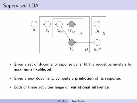
Supervised LDA
!d Zd,n Wd,nN
D
K!k
!
Yd !, "2
• Given a set of document-response pairs, fit the model parameters bymaximum likelihood.
• Given a new document, compute a prediction of its response.
• Both of these activities hinge on variational inference.
D. Blei Topic Models
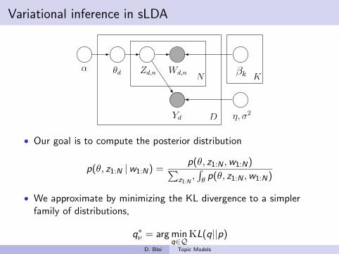
Variational inference in sLDA
!d Zd,n Wd,nN
D
K!k
!
Yd !, "2
• Our goal is to compute the posterior distribution
p(θ, z1:N |w1:N) =p(θ, z1:N ,w1:N)∑
z1:N,∫θ p(θ, z1:N ,w1:N)
• We approximate by minimizing the KL divergence to a simplerfamily of distributions,
q∗ν = arg minq∈Q
KL(q||p)
D. Blei Topic Models

Variational inference in sLDA
!d Zd,n Wd,nN
D
K!k
!
Yd !, "2
Equivalently, maximize the Jensen’s bound
log p(w1:N , y) ≥E[log p(θ |α)] +
∑Nn=1 E[log p(Zn | θ)] +
∑Nn=1 E[log p(wn |Zn, β1:K )]
+E[log p(y |Z1:N , η, σ2)] + H(q)
D. Blei Topic Models

Variational inference in sLDA
!d Zd,n Wd,nN
D
K!k
!
Yd !, "2
The distinguishing term is
E[log p(y |Z1:N)] = −1
2log(2πσ2
)− y2 − 2yη>E
[Z̄]
+ η>E[Z̄ Z̄>
]η
2σ2
We use the fully-factorized variational distribution
q(θ, z1:N | γ, φ1:N) = q(θ | γ)∏N
n=1 q(zn |φn),
D. Blei Topic Models

Variational inference in sLDA
!d Zd,n Wd,nN
D
K!k
!
Yd !, "2
• The expectations are
E[Z̄]
= φ̄ :=1
N
N∑
n=1
φn
E[Z̄ Z̄>
]=
1
N2
(∑Nn=1
∑m 6=n φnφ
>m +
∑Nn=1 diag{φn}
).
• Leads to an easy coordinate ascent algorithm.
D. Blei Topic Models

Maximum likelihood estimation
• The M-step is an MLE under expected sufficient statistics.
• Define
• y = y1:D is the response vector• A is the D × K matrix whose rows are Z̄>d .
• MLE of the coefficients solve the expected normal equations
E[A>A
]η = E[A]>y ⇒ η̂new ←
(E[A>A
])−1E[A]>y
• The MLE of the variance is
σ̂2new ← (1/D){y>y − y>E[A]
(E[A>A
])−1E[A]>y}
D. Blei Topic Models

Prediction
• We have fit SLDA parameters to a corpus, using variational EM.
• We have a new document w1:N with unknown response value.
• First, run variational inference in the unsupervised LDA model, toobtain γ and φ1:N for the new document.(LDA ⇔ integrating unobserved Y out of SLDA.)
• Predict y using SLDA expected value:
E[Y |w1:N , α, β1:K , η, σ
2]≈ η>Eq
[Z̄]
= η>φ̄.
D. Blei Topic Models

Example: Movie reviews
bothmotionsimpleperfectfascinatingpowercomplex
howevercinematographyscreenplayperformancespictureseffectivepicture
histheircharactermanywhileperformancebetween
−30 −20 −10 0 10 20
● ●● ● ●● ● ● ● ●
morehasthanfilmsdirectorwillcharacters
onefromtherewhichwhomuchwhat
awfulfeaturingroutinedryofferedcharlieparis
notaboutmovieallwouldtheyits
havelikeyouwasjustsomeout
badguyswatchableitsnotonemovie
leastproblemunfortunatelysupposedworseflatdull
• 10-topic sLDA model on movie reviews (Pang and Lee, 2005).
• Response: number of stars associated with each review
• Each component of coefficient vector η is associated with a topic.
D. Blei Topic Models

Predictive R2
(SLDA is red.)
●
●
● ●● ● ● ●
●●
●
●
●● ●
●● ● ●
●
5 10 15 20 25 30 35 40 45 50
0.0
0.1
0.2
0.3
0.4
0.5
Number of topics
Pre
dict
ive
R2
D. Blei Topic Models

Held out likelihood
(SLDA is red.)
●● ●
●
●
●
●
●
●
●
●
●
● ●
●
●
●
●
●
●
5 10 15 20 25 30 35 40 45 50
−6.
42−
6.41
−6.
40−
6.39
−6.
38−
6.37
Number of topics
Per
−w
ord
held
out
log
likel
ihoo
d
D. Blei Topic Models

Predictive R2 on Digg
(SLDA is red.)
●
● ●
●
●●
●
●
●
●●
●●
●
2 4 10 20 30
0.00
0.02
0.04
0.06
0.08
0.10
0.12
Number of topics
Pre
dict
ive
R2
D. Blei Topic Models

Held out likelihood on Digg
(SLDA is red.)
● ● ●●
●
●
●
●
●● ●
●
●
●
2 4 10 20 30
−8.
6−
8.5
−8.
4−
8.3
−8.
2−
8.1
−8.
0
Number of topics
Per
−w
ord
held
out
log
likel
ihoo
d
D. Blei Topic Models

Diverse response types with GLMs
• Want to work with response variables that don’t live in the reals.
• binary / multiclass classification• count data• waiting time
• Model the response response with a generalized linear model
p(y | ζ, δ) = h(y , δ) exp
{ζy − A(ζ)
δ
},
where ζ = η>z̄ .
• Complicates inference, but allows for flexible modeling.
D. Blei Topic Models

Example: Multi-class classification
756757758759760761762763764765766767768769770771772773774775776777778779780781782783784785786787788789790791792793794795796797798799800801802803804805806807808809
810811812813814815816817818819820821822823824825826827828829830831832833834835836837838839840841842843844845846847848849850851852853854855856857858859860861862863
CVPR#318
CVPR#318
CVPR 2009 Submission #318. CONFIDENTIAL REVIEW COPY. DO NOT DISTRIBUTE.
highway
car, sign, road
coast (highway)
car, sand beach, tree
inside city
buildings, car, sidewalk
street (inside city)
window, tree, building
occluded
tall building
trees, buildings
occluded, window
inside city (tall building)
tree, car, sidewalk
street
tree, car, sidewalk
highway (street)
car, window, tree
forest
tree trunk, trees,
ground grass
mountain (forest)
snowy mountain, tree
trunk
coast
sand beach, cloud
open country (coast)
sea water, buildings
mountain
snowy mountain,
sea water, field
highway (mountain)
tree, snowy mountain
open country
cars, field,
sand beach
coast (open country)
tree, field, sea water
Incorrect classification (correct class)
with predicted annotations
Correct classification
with predicted annotations
Figure 4. Example results from the LabelMe dataset. For each class, left side contains examples with correct classification and predictedannotations, while right side contains wrong ones (the class label in the bracket is the right one) with the predicted annotations. The italicwords indicate the class label, while the normal words are associated predicted annotations.
[28] J. Vogel and B. Schiele. A semantic typicality measure fornatural scene categorization. In DAGM-Symposium, 2004. 5
[29] Y. Wang and S. Gong. Conditional random field for naturalscene categorization. In BMVC, 2007. 5
[30] Z.-H. Zhou and M.-L. Zhang. Multi-instance multi-labellearning with application to scene classification. In NIPS,2006. 5
8
540541542543544545546547548549550551552553554555556557558559560561562563564565566567568569570571572573574575576577578579580581582583584585586587588589590591592593
594595596597598599600601602603604605606607608609610611612613614615616617618619620621622623624625626627628629630631632633634635636637638639640641642643644645646647
CVPR#318
CVPR#318
CVPR 2009 Submission #318. CONFIDENTIAL REVIEW COPY. DO NOT DISTRIBUTE.
20 40 60 80 100 120
0.64
0.66
0.68
0.7
0.72
0.74
0.76
0.78
topics
ave
rag
e a
ccu
racy
image classification on the LabelMe dataset
multi!class sLDA with annotations multi!class sLDA Fei!Fei and Perona, 2005 Bosch et al., 2006
20 40 60 80 100 120
0.56
0.58
0.6
0.62
0.64
0.66
topics
ave
rag
e a
ccu
racy
image classification on the UIUC!Sport dataset
Figure 2. Comparisons of average accuracy over all classes based on 5 random train/test subsets. multi-class sLDA with annotations andmulti-class sLDA (red curves in color) are both our models. left. Accuracy as a function of the number of topics on the LabelMe dataset.right. Accuracy as a function of the number of topics on the UIUC-Sport dataset.
3. multi-class sLDA: This is the multi-class sLDA model,described in this paper.
4. multi-class sLDA with annotations: This is multi-classsLDA with annotations, described in this paper.
Note all testing is performed on unlabeled and unannotatedimages.
The results are illustrated in the graphs of Figure 2 andin the confusion matrices of Figure 3.2 Our models—multi-class sLDA and multi-class sLDA with annotations— per-form better than the other approaches. They reduce the errorof Fei-Fei and Perona, 2005 by at least 10% on both datasets, and even more for Bosch et al., 2006. This demon-strates that multi-class sLDA is a better classifier, and thatjoint modeling does not negatively affect classification ac-curacy when annotation information is available. In fact, itusually increases the accuracy.
Observe that the model of [5], unsupervised LDA com-bined with KNN, gives the worst performance of thesemethods. This highlights the difference between findingtopics that are predictive, as our models do, and findingtopics in an unsupervised way. The accuracy of unsuper-vised LDA might be increased by using some of the othervisual features suggested by [5]. Here, we restrict ourselvesto SIFT features in order to compare models, rather thanfeature sets.
As the number of topics increases, the multi-class sLDAmodels (with and without annotation) do not overfit untilaround 100 topics, while Fei-Fei and Perona, 2005 beginsto overfit at 40 topics. This suggests that multi-class sLDA,which combines aspects of both generative and discrimina-tive classification, can handle more latent features than a
2Other than the topic models listed, we also tested an SVM-based ap-proach using SIFT image features. The SVM yielded much worse perfor-mance than the topic models (47% for the LabelMe data, and 20% for theUIUC-Sport data). These are not marked on the plots.
purely generative approach. On one hand, a large numberof topics increases the possibility of overfitting; on the otherhand, it provides more latent features for building the clas-sifier.
Image Annotation. In the case of multi-class sLDA withannotations, we can use the same trained model for imageannotation. We emphasize that our models are designed forsimultaneous classification and annotation. For image an-notation, we compare following two methods,
1. Blei and Jordan, 2003: This is the corr-LDA modelfrom [2], trained on annotated images.
2. multi-class sLDA with annotations: This is exactly thesame model trained for image classification in the pre-vious section. In testing annotation, we observe onlyimages.
To measure image annotation performance, we use anevaluation measure from information retrieval. Specifi-cally, we examine the top-N F-measure3, denoted as F-measure@N , where we set N = 5. We find that multi-class sLDA with annotations performs slightly better thancorr-LDA over all the numbers of topics tested (about 1%relative improvement). For example, considering modelswith 100 topics, the LabelMe F-measures are 38.2% (corr-LDA) and 38.7% (multi-class sLDA with annotations); onUIUC-Sport, they are 34.7% (corr-LDA) and 35.0% (multi-class sLDA with annotations).
These results demonstrate that our models can performclassification and annotation with the same latent space.With a single trained model, we find the annotation per-formance that is competitive with the state-of-the-art, andclassification performance that is superior.
3F-measure is defined as 2 ! precision ! recall/(precision + recall).
6
# of components
SLDA for image classification (with Chong Wang, CVPR 2009)
D. Blei Topic Models

Supervised topic models
• SLDA enables model-based regression where the predictor “variable”is a text document.
• It can easily be used wherever LDA is used in an unsupervisedfashion (e.g., images, genes, music).
• SLDA is a supervised dimension-reduction technique, whereas LDAperforms unsupervised dimension reduction.
• LDA + regression compared to sLDA is like principal componentsregression compared to partial least squares.
D. Blei Topic Models
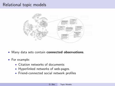
Relational topic models
52
478
430
2487
75
288
1123
2122
2299
1354
1854
1855
89
635
92
2438
136
479
109
640
119686
120
1959
1539
147
172
177
965
911
2192
1489
885
178378
286
208
1569
2343
1270
218
1290
223
227
236
1617
254
1176
256
634
264
1963
2195
1377
303
426
2091
313
1642
534
801
335
344
585
1244
2291
2617
1627
2290
1275
375
1027
396
1678
2447
2583
1061 692
1207
960
1238
20121644
2042
381
418
1792
1284
651
524
1165
2197
1568
2593
1698
547 683
2137 1637
2557
2033632
1020
436442
449
474
649
2636
2300
539
541
603
1047
722
660
806
1121
1138
831837
1335
902
964
966
981
16731140
14811432
1253
1590
1060
992
994
1001
1010
1651
1578
1039
1040
1344
1345
1348
1355
14201089
1483
1188
1674
1680
2272
1285
1592
1234
1304
1317
1426
1695
1465
1743
1944
2259
2213
We address the problem of finding a subset of features that allows a supervised induction algorithm to induce small high-accuracy concepts...
Irrelevant features and the subset selection problem
In many domains, an appropriate inductive bias is the MIN-FEATURES bias, which prefers consistent hypotheses definable over as few features as possible...
Learning with many irrelevant features
In this introduction, we define the term bias as it is used in machine learning systems. We motivate the importance of automated methods for evaluating...
Evaluation and selection of biases in machine learning
The inductive learning problem consists of learning a concept given examples and nonexamples of the concept. To perform this learning task, inductive learning algorithms bias their learning method...
Utilizing prior concepts for learning
The problem of learning decision rules for sequential tasks is addressed, focusing on the problem of learning tactical plans from a simple flight simulator where a plane must avoid a missile...
Improving tactical plans with genetic algorithms
Evolutionary learning methods have been found to be useful in several areas in the development of intelligent robots. In the approach described here, evolutionary...
An evolutionary approach to learning in robots
Navigation through obstacles such as mine fields is an important capability for autonomous underwater vehicles. One way to produce robust behavior...
Using a genetic algorithm to learn strategies for collision
avoidance and local navigation
...
...
...
...
...
...
...
...
...
...
• Many data sets contain connected observations.
• For example:
• Citation networks of documents• Hyperlinked networks of web-pages.• Friend-connected social network profiles
D. Blei Topic Models

Relational topic models
52
478
430
2487
75
288
1123
2122
2299
1354
1854
1855
89
635
92
2438
136
479
109
640
119686
120
1959
1539
147
172
177
965
911
2192
1489
885
178378
286
208
1569
2343
1270
218
1290
223
227
236
1617
254
1176
256
634
264
1963
2195
1377
303
426
2091
313
1642
534
801
335
344
585
1244
2291
2617
1627
2290
1275
375
1027
396
1678
2447
2583
1061 692
1207
960
1238
20121644
2042
381
418
1792
1284
651
524
1165
2197
1568
2593
1698
547 683
2137 1637
2557
2033632
1020
436442
449
474
649
2636
2300
539
541
603
1047
722
660
806
1121
1138
831837
1335
902
964
966
981
16731140
14811432
1253
1590
1060
992
994
1001
1010
1651
1578
1039
1040
1344
1345
1348
1355
14201089
1483
1188
1674
1680
2272
1285
1592
1234
1304
1317
1426
1695
1465
1743
1944
2259
2213
We address the problem of finding a subset of features that allows a supervised induction algorithm to induce small high-accuracy concepts...
Irrelevant features and the subset selection problem
In many domains, an appropriate inductive bias is the MIN-FEATURES bias, which prefers consistent hypotheses definable over as few features as possible...
Learning with many irrelevant features
In this introduction, we define the term bias as it is used in machine learning systems. We motivate the importance of automated methods for evaluating...
Evaluation and selection of biases in machine learning
The inductive learning problem consists of learning a concept given examples and nonexamples of the concept. To perform this learning task, inductive learning algorithms bias their learning method...
Utilizing prior concepts for learning
The problem of learning decision rules for sequential tasks is addressed, focusing on the problem of learning tactical plans from a simple flight simulator where a plane must avoid a missile...
Improving tactical plans with genetic algorithms
Evolutionary learning methods have been found to be useful in several areas in the development of intelligent robots. In the approach described here, evolutionary...
An evolutionary approach to learning in robots
Navigation through obstacles such as mine fields is an important capability for autonomous underwater vehicles. One way to produce robust behavior...
Using a genetic algorithm to learn strategies for collision
avoidance and local navigation
...
...
...
...
...
...
...
...
...
...
• Research has focused on finding communities and patterns in thelink-structure of these networks (Kemp et al. 2004, Hoff et al.,2002, Hofman and Wiggins 2007, Airoldi et al. 2008).
• By adapting supervised topic modeling, we can build a good modelof content and structure.
• RTMs find related hidden structure in both types of data.D. Blei Topic Models

Relational topic models
α
Nd
θd
wd,n
zd,n
Kβk
yd,d'
η
Nd'
θd'
wd',n
zd',n
• Binary response variable with each pair of documents
• Adapt variational EM algorithm for sLDA with binary GLM responsemodel (with different link probability functions).
• Allows predictions that are out of reach for traditional models.
D. Blei Topic Models

Predictive performance of one type given the other
5 10 15 20 25
!3600
!3550
!3500
!3450
Cora
Number of topics
Wo
rd L
og
Lik
elih
oo
d5 10 15 20 25
!14000
!13500
!13000
Cora
Number of topics
Lin
k L
og
Lik
elih
oo
d
RTM,, !!""
RTM,, !!e
LDA + Regression
Mixed!Membership
Unigram/Bernoulli
Cora corpus (McCallum et al., 2000)
D. Blei Topic Models

Predictive performance of one type given the other
5 10 15 20 25
!3350
!3300
!3250
!3200
WebKB
Number of topics
Lin
k L
og
Lik
elih
oo
d
5 10 15 20 25!1145
!1140
!1135
!1130
WebKB
Number of topics
Wo
rd L
og
Lik
elih
oo
d
RTM,, !!""
RTM,, !!e
LDA + Regression
Mixed!Membership
Unigram/Bernoulli
WebKB corpus (Craven et al., 1998)
D. Blei Topic Models

Predictive performance of one type given the other
5 10 15 20 25
!4750
!4700
!4650
!4600
!4550
!4500
!4450
PNAS
Number of topics
Lin
k L
og
Lik
eli
ho
od
5 10 15 20 25!2970
!2960
!2950
!2940
PNAS
Number of topics
Wo
rd L
og
Lik
elih
oo
d
RTM,, !!""
RTM,, !!e
LDA + Regression
Mixed!Membership
Unigram/Bernoulli
PNAS corpus (courtesy of JSTOR)
D. Blei Topic Models

Predicting links from documents
16 J. CHANG AND D. BLEI
Table 2Top eight link predictions made by RTM (!e) and LDA + Regression for two documents(italicized) from Cora. The models were fit with 10 topics. Boldfaced titles indicate actual
documents cited by or citing each document. Over the whole corpus, RTM improvesprecision over LDA + Regression by 80% when evaluated on the first 20 documents
retrieved.
Markov chain Monte Carlo convergence diagnostics: A comparative review
Minorization conditions and convergence rates for Markov chain Monte Carlo
RT
M(!
e)
Rates of convergence of the Hastings and Metropolis algorithmsPossible biases induced by MCMC convergence diagnostics
Bounding convergence time of the Gibbs sampler in Bayesian image restorationSelf regenerative Markov chain Monte Carlo
Auxiliary variable methods for Markov chain Monte Carlo with applicationsRate of Convergence of the Gibbs Sampler by Gaussian Approximation
Diagnosing convergence of Markov chain Monte Carlo algorithms
Exact Bound for the Convergence of Metropolis Chains LD
A+
Regressio
n
Self regenerative Markov chain Monte CarloMinorization conditions and convergence rates for Markov chain Monte Carlo
Gibbs-markov modelsAuxiliary variable methods for Markov chain Monte Carlo with applications
Markov Chain Monte Carlo Model Determination for Hierarchical and Graphical ModelsMediating instrumental variables
A qualitative framework for probabilistic inferenceAdaptation for Self Regenerative MCMC
Competitive environments evolve better solutions for complex tasks
Coevolving High Level Representations
RT
M(!
e)
A Survey of Evolutionary StrategiesGenetic Algorithms in Search, Optimization and Machine Learning
Strongly typed genetic programming in evolving cooperation strategiesSolving combinatorial problems using evolutionary algorithms
A promising genetic algorithm approach to job-shop scheduling. . .Evolutionary Module Acquisition
An Empirical Investigation of Multi-Parent Recombination Operators. . .
A New Algorithm for DNA Sequence Assembly
LD
A+
Regressio
n
Identification of protein coding regions in genomic DNASolving combinatorial problems using evolutionary algorithms
A promising genetic algorithm approach to job-shop scheduling. . .A genetic algorithm for passive management
The Performance of a Genetic Algorithm on a Chaotic Objective FunctionAdaptive global optimization with local search
Mutation rates as adaptations
Table 2 illustrates suggested citations using RTM (!e) and LDA + Regres-sion as predictive models. These suggestions were computed from a model fiton one of the folds of the Cora data. The top results illustrate suggested linksfor “Markov chain Monte Carlo convergence diagnostics: A comparative re-
Given a new document, which documents is it likely to link to?
D. Blei Topic Models

Spatially consistent topics18 J. CHANG AND D. BLEI
Topic 1
Topic 2
Topic 3
Topic 4
Topic 5
Topic 1
Topic 2
Topic 3
Topic 4
Topic 5
Fig 5. A comparison between RTM (left) and LDA (right) of topic distributions on localnews data. Each color/row depicts a single topic. Each state’s color intensity indicates themagnitude of that topic’s component. The corresponding words associated with each topicare given in Table 3. Whereas LDA finds geographically di!use topics, RTM, by modelingspatial connectivity, finds coherent regions.
18 J. CHANG AND D. BLEI
Topic 1
Topic 2
Topic 3
Topic 4
Topic 5
Topic 1
Topic 2
Topic 3
Topic 4
Topic 5
Fig 5. A comparison between RTM (left) and LDA (right) of topic distributions on localnews data. Each color/row depicts a single topic. Each state’s color intensity indicates themagnitude of that topic’s component. The corresponding words associated with each topicare given in Table 3. Whereas LDA finds geographically di!use topics, RTM, by modelingspatial connectivity, finds coherent regions.
• For exploratory tasks, RTMs can be used to “guide” the topics
• Documents are geographically-tagged news articles from Yahoo!Links are the adjacency matrix of states
• RTM finds spatially consistent topics.D. Blei Topic Models

Relational Topic Models
• Relational topic modeling allows us to analyze connecteddocuments, or other data for which the mixed-membershipassumptions are appropriate.
• Traditional models cannot predict with new and unlinked data.
• RTMs allow for such predictions
• links given the new words of a document• words given the links of a new document
D. Blei Topic Models

Used in exploratory tools of document collections
D. Blei Topic Models