EXCESS RISK BOUNDS IN

MACHINE LEARNING

VLADIMIR KOLTCHINSKII

School of Mathematics

Georgia Institute of Technology

Theory and Practice of Computational Learning

Summer School, Chicago, 2009

TOPICS

• Basic Inequalities for Empirical Processes

• Distribution Dependent Bounds on Excess Risk

• Rademacher Complexities and Data Dependent Bounds

on Excess Risk

• Penalized Empirical Risk Minimization and Oracle

Inequalities

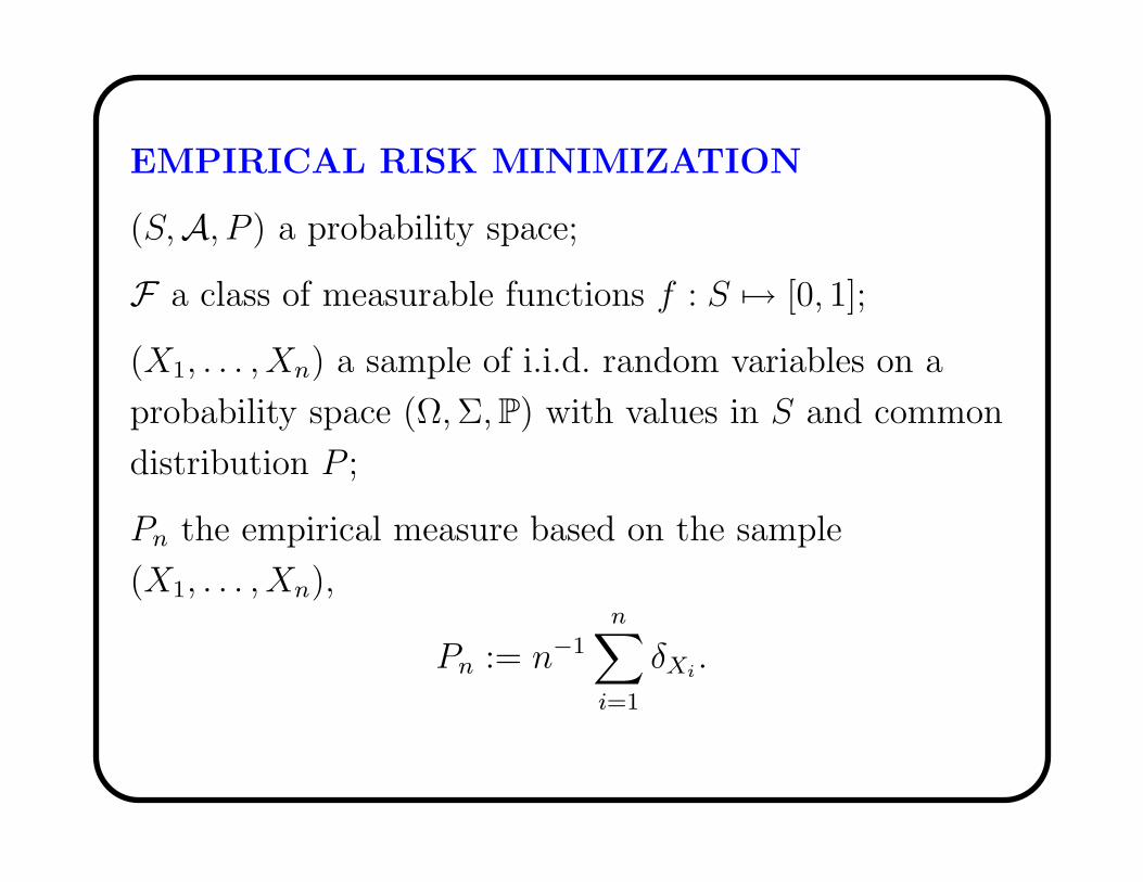
EMPIRICAL RISK MINIMIZATION

(S,A, P ) a probability space;

F a class of measurable functions f : S 7→ [0, 1];

(X1, . . . , Xn) a sample of i.i.d. random variables on a

probability space (Ω,Σ,P) with values in S and common

distribution P ;

Pn the empirical measure based on the sample

(X1, . . . , Xn),

Pn := n−1

n∑

i=1

δXi.

Risk minimization:

Pf :=

∫

S

fdP = Ef(X) −→ min, f ∈ F (1)

Empirical risk minimization (ERM):

Pnf :=

∫

S

fdPn = n−1

n∑

j=1

f(Xj) −→ min, f ∈ F . (2)

Empirical risk minimizer: a solution fn of (2).

Excess risk:

E(f) := EP (f) := Pf − inff∈F

Pf.

Problems:

• distribution dependent and data dependent bounds on

E(fn) that take into account the ”geometry” of F ;

• given a family (a ”sieve”) F1,F2, · · · ⊂ F of function

classes approximating F and a sequence fn,k of empirical

risk minimizers on each class, to construct

f = fn,k ∈ Fk ⊂ F

with a ”nearly optimal” excess risk (model selection

problem).

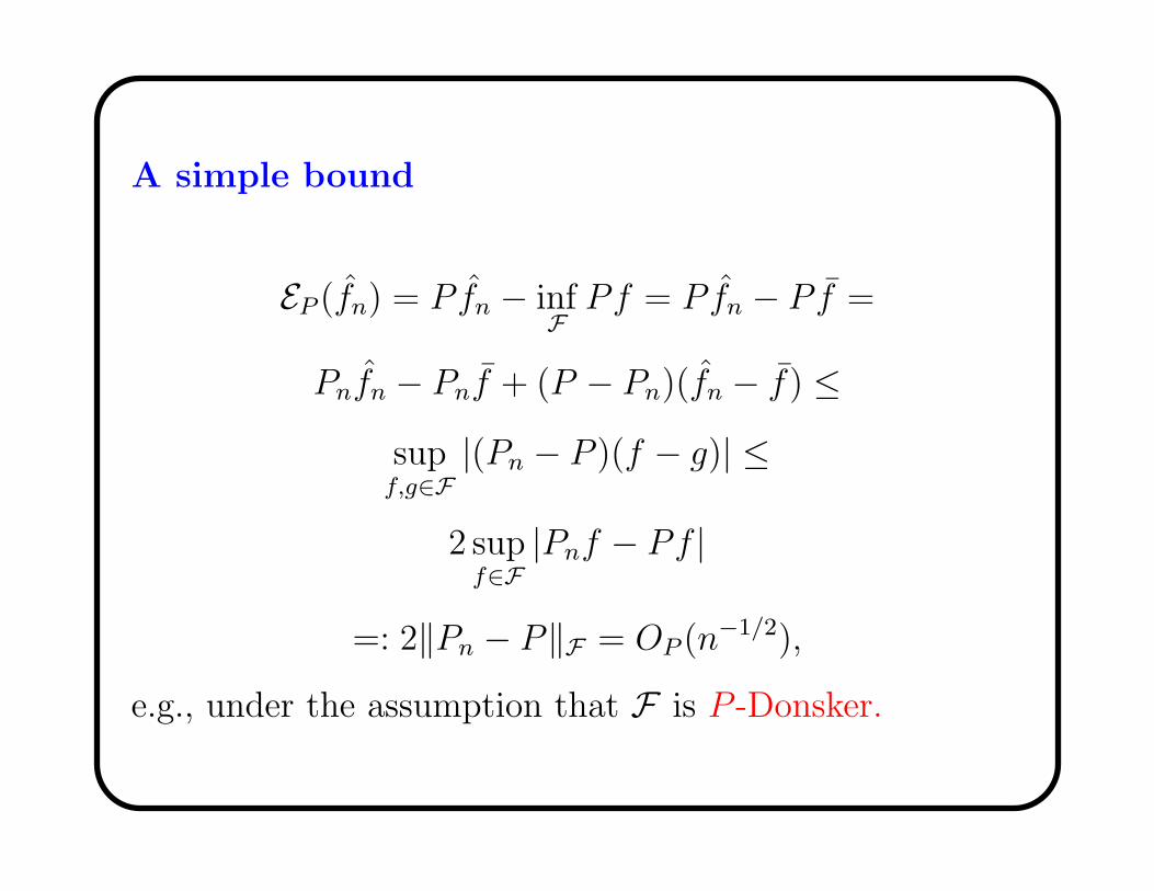
A simple bound

EP (fn) = P fn − infFPf = P fn − P f =

Pnfn − Pnf + (P − Pn)(fn − f) ≤

supf,g∈F

|(Pn − P )(f − g)| ≤

2 supf∈F

|Pnf − Pf |

=: 2‖Pn − P‖F = OP (n−1/2),

e.g., under the assumption that F is P -Donsker.

Specific bounds under various complexity assumptions on

the class follow from the results of empirical processes

theory:

Vapnik and Chervonenkis, Dudley, Koltchinskii,

Pollard, Gine and Zinn, Alexander, Massart, Talagrand,

Ledoux

However, the convergence rate O(n−1/2) most often is not

sharp. In the case of P -Donsker class F , EP (fn)

converges to 0 typically as fast as oP (n−1/2). Sometimes,

the convergence rate is as fast as OP (n−1).

Empirical and Rademacher Processes

Empirical Process

Pnf − Pf, f ∈ F

Basic Questions

• What is the size of

‖Pn − P‖F := supf∈F

|Pnf − Pf |?

• Does it depend on the “complexity” of F and on the

unknown distribution P, and how?

• How to estimate this quantity based on the data?

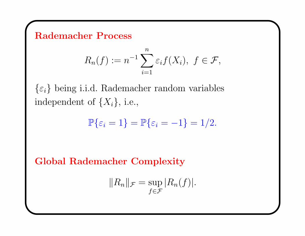
Rademacher Process

Rn(f) := n−1

n∑

i=1

εif(Xi), f ∈ F ,

εi being i.i.d. Rademacher random variables

independent of Xi, i.e.,

Pεi = 1 = Pεi = −1 = 1/2.

Global Rademacher Complexity

‖Rn‖F = supf∈F

|Rn(f)|.

Symmetrization Inequality

1

2E‖Rn‖Fc ≤ E‖Pn − P‖F ≤ 2E‖Rn‖F ,

where Fc = f − Pf : f ∈ F.

Contraction Inequality

For F with values in [−1, 1], ϕ a function on [−1, 1] with

ϕ(0) = 0 and ϕ Lipschitz with constant 1, and for

ϕ F := ϕ f : f ∈ F,

E‖Rn‖ϕF ≤ 2E‖Rn‖F .

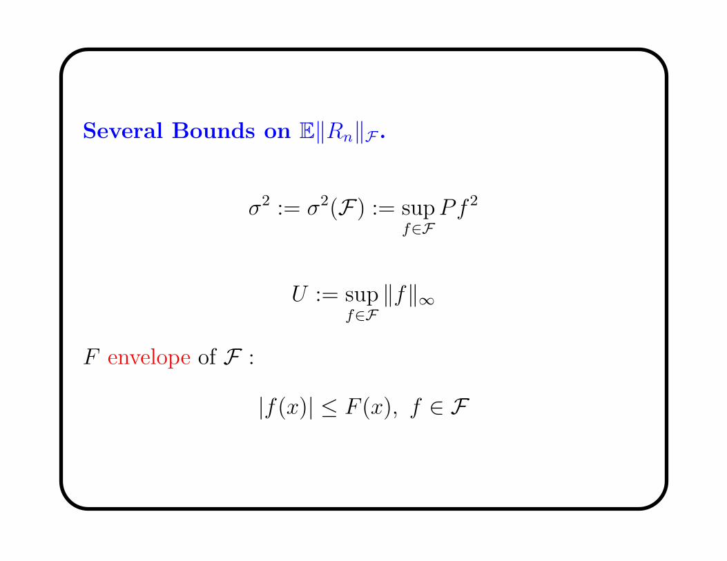
Several Bounds on E‖Rn‖F .

σ2 := σ2(F) := supf∈F

Pf 2

U := supf∈F

‖f‖∞

F envelope of F :

|f(x)| ≤ F (x), f ∈ F

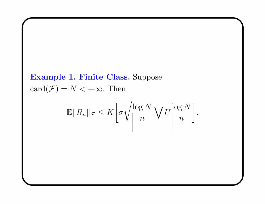
Example 1. Finite Class. Suppose

card(F) = N < +∞. Then

E‖Rn‖F ≤ K

[

σ

√

logN

n

∨

UlogN

n

]

.

Example 2. Shattering Numbers. Suppose F is a

class of functions f : S 7→ 0, 1,

∆F(X1, . . . , Xn) :=

card

(

(f(X1), . . . , f(Xn)) : f ∈ F)

.

Then

E‖Rn‖F ≤

K

[

σE

√

log ∆F(X1, . . . , Xn)

n

∨

Elog ∆F(X1, . . . , Xn)

n

]

.

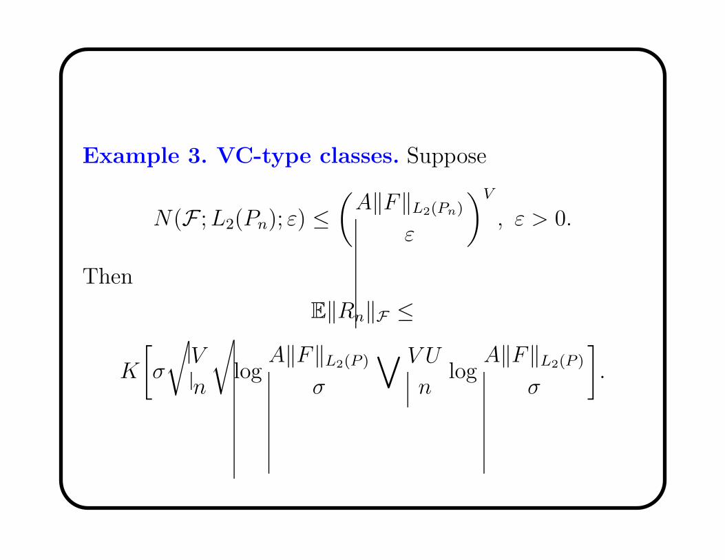
Example 3. VC-type classes. Suppose

N(F ;L2(Pn); ε) ≤(

A‖F‖L2(Pn)

ε

)V

, ε > 0.

Then

E‖Rn‖F ≤

K

[

σ

√

V

n

√

logA‖F‖L2(P )

σ

∨ V U

nlog

A‖F‖L2(P )

σ

]

.

Example 4. Larger Entropy. Suppose that for some

ρ ∈ (0, 1)

logN(F ;L2(Pn); ε) ≤(

A‖F‖L2(Pn)

ε

)2ρ

, ε > 0.

Then

E‖Rn‖F ≤

K

[

σ1−ρAρ‖F‖ρ

L2(P )

n1/2

∨ A2ρ/(ρ+1)‖F‖2ρ/(ρ+1)L2(P ) U (1−ρ)/(1+ρ)

n1/(1+ρ)

]

.

Example 6. Subsets of RKHS. Let K be a symmetric

nonnegatively definite kernel on S × S and HK be the

corresponding reproducing kernel Hilbert space (RKHS).

Suppose

F ⊂ f : ‖f‖HK≤ 1.

Denote λj the eigenvalues of the integral operator from

L2(P ) into L2(P ) with kernel K. Then

E‖Rn‖F ≤ C

(

n−1

∞∑

j=1

(λj ∧ σ2)

)1/2

.

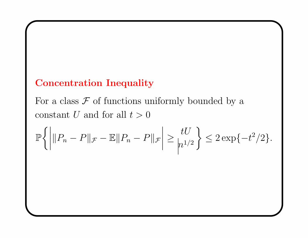
Concentration Inequality

For a class F of functions uniformly bounded by a

constant U and for all t > 0

P

∣

∣

∣

∣

‖Pn − P‖F − E‖Pn − P‖F∣

∣

∣

∣

≥ tU

n1/2

≤ 2 exp−t2/2.

Comparison of Empirical and Rademacher

Processes

For all t > 0

P

‖Pn − P‖F ≥ 2‖Rn‖F +3tU√n

≤ exp−t2/2

with a similar lower bound.

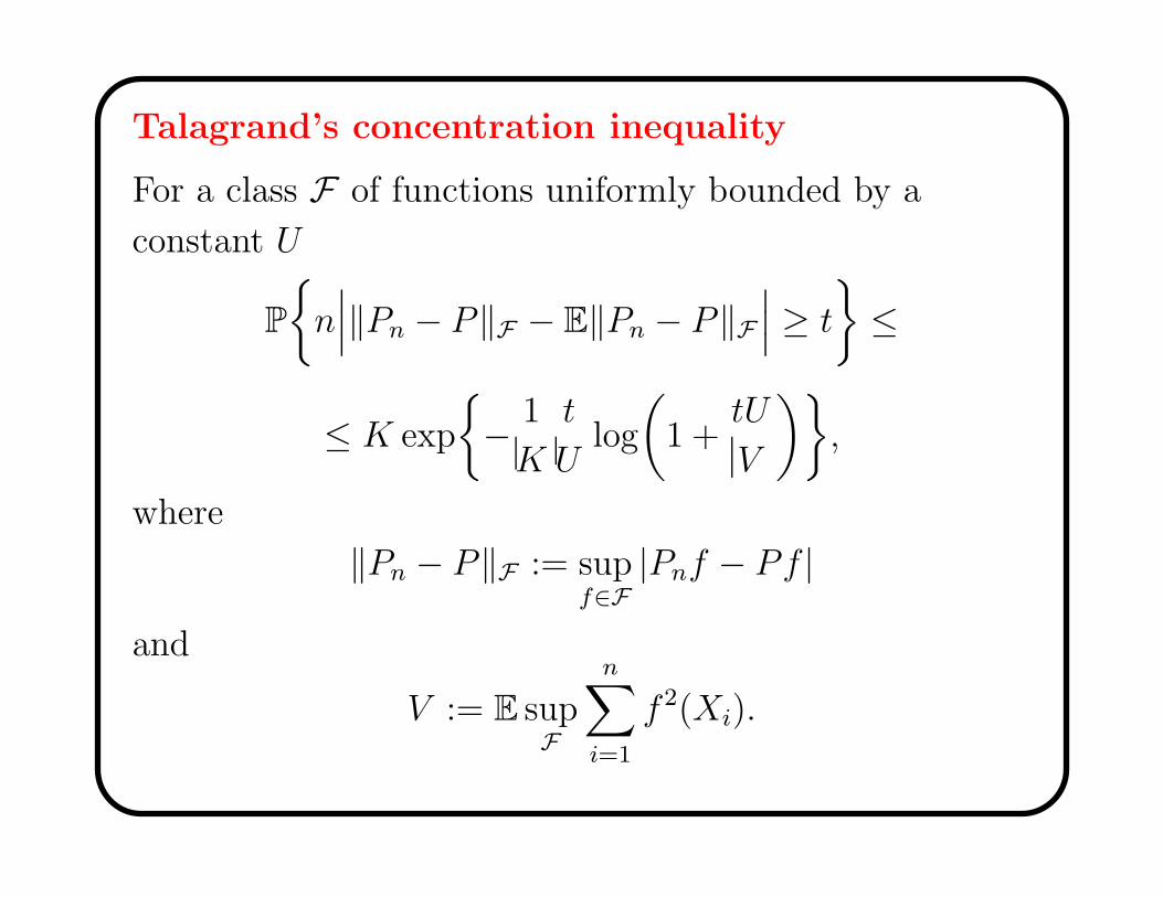
Talagrand’s concentration inequality

For a class F of functions uniformly bounded by a

constant U

P

n∣

∣

∣‖Pn − P‖F − E‖Pn − P‖F

∣

∣

∣≥ t

≤

≤ K exp

− 1

K

t

Ulog

(

1 +tU

V

)

,

where

‖Pn − P‖F := supf∈F

|Pnf − Pf |

and

V := E supF

n∑

i=1

f 2(Xi).

It is often used in combination with

E supF

n∑

i=1

f 2(Xi) ≤ nσ2(F) + 8UE supF

∣

∣

∣

∣

n∑

i=1

εif(Xi)

∣

∣

∣

∣

,

where σ2(F) := supf∈F Pf2 and εi are i.i.d.

Rademacher r.v. independent of Xi, which yields the

following: with probability at least 1 − e−t

∣

∣

∣

∣

‖Pn − P‖F − E‖Pn − P‖F∣

∣

∣

∣

≤

K

[

√

t

n

(

σ2(F) + UE‖Rn‖F)

+tU

n

]

.

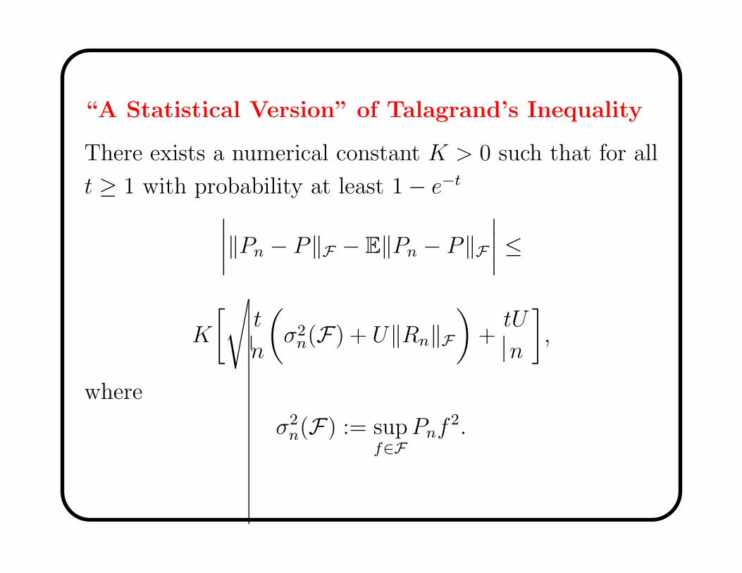
“A Statistical Version” of Talagrand’s Inequality

There exists a numerical constant K > 0 such that for all

t ≥ 1 with probability at least 1 − e−t

∣

∣

∣

∣

‖Pn − P‖F − E‖Pn − P‖F∣

∣

∣

∣

≤

K

[

√

t

n

(

σ2n(F) + U‖Rn‖F

)

+tU

n

]

,

where

σ2n(F) := sup

f∈FPnf

2.

The same bounds hold for∣

∣

∣

∣

‖Rn‖F − E‖Rn‖F∣

∣

∣

∣

.

Distribution Dependent Excess Risk Bounds

References:

Massart (2000, 2007),

Koltchinskii and Panchenko (2000),

Bousquet, Koltchinskii and Panchenko (2002),

Bartlett, Bousquet and Mendelson (2002, 2005),

Koltchinskii (2006, 2008),

Bartlett and Mendelson (2006)

Some Definitions

Empirical excess risk:

En(f) := EPn(f) := Pnf − infFPnf ;

δ-minimal sets:

F(δ) := FP (δ) :=

f ∈ F : EP (f) ≤ δ

,

Fn(δ) := FPn(δ).

L2-diameter:

D(δ) := DP (δ) := supf,g∈F(δ)

(P (f − g)2)1/2

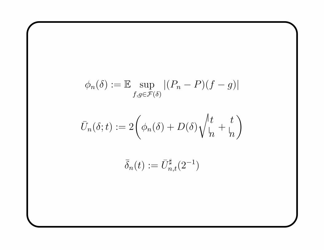
A measure of empirical approximation:

φn(δ) := E supf,g∈F(δ)

|(Pn − P )(f − g)|.

Define

Un(δ; t) := 2

(

φn(δ) +D(δ)

√

t

n+t

n

)

.

A consequence of Talagrand’s inequality (Bousquet’s

version):

P

supf,g∈F(δ)

|(Pn − P )(f − g)| ≥ Un(δ; t)

≤ e−t.

Reminder: a simple bound

EP (fn) = P fn − infFPf = P fn − P f =

Pnfn − Pnf + (P − Pn)(fn − f) ≤

supf,g∈F

|(Pn − P )(f − g)|.

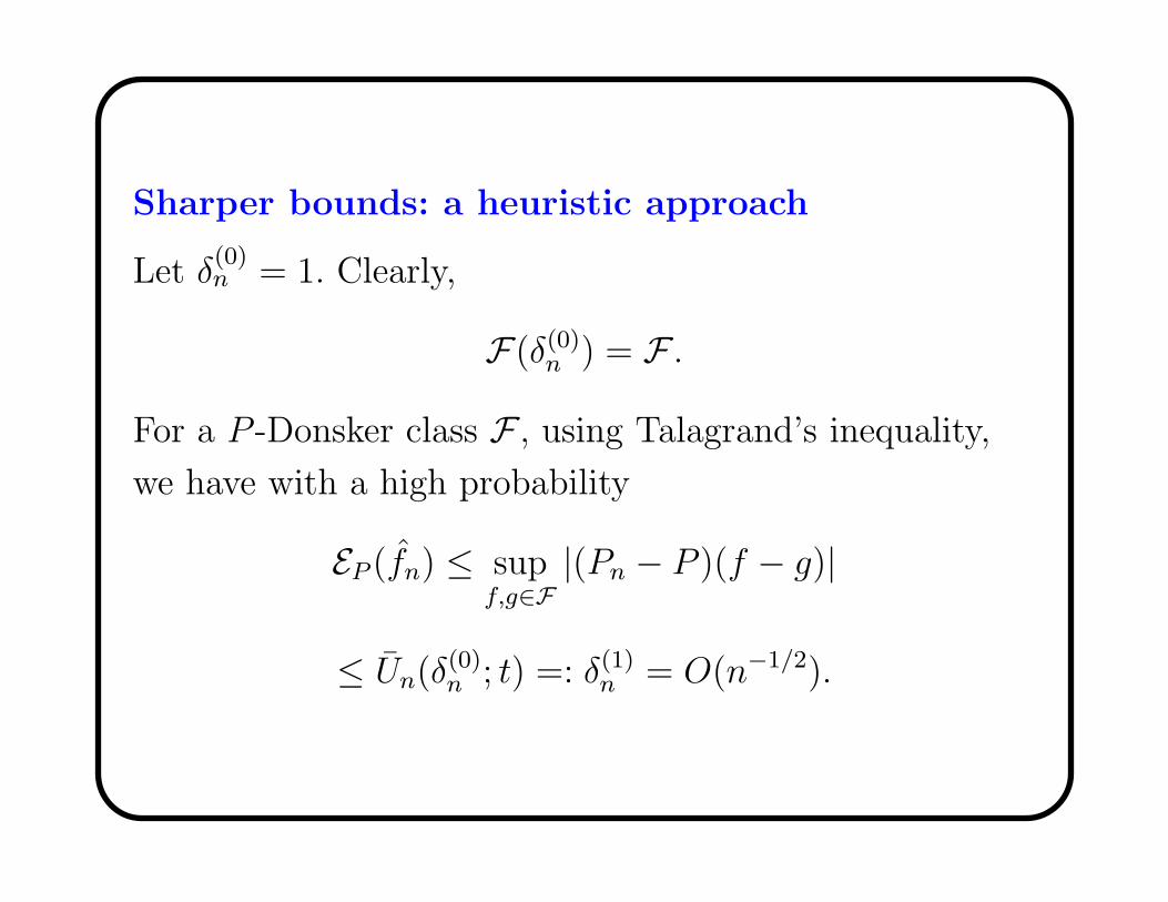
Sharper bounds: a heuristic approach

Let δ(0)n = 1. Clearly,

F(δ(0)n ) = F .

For a P -Donsker class F , using Talagrand’s inequality,

we have with a high probability

EP (fn) ≤ supf,g∈F

|(Pn − P )(f − g)|

≤ Un(δ(0)n ; t) =: δ(1)

n = O(n−1/2).

Then the same argument as before shows that with a

high probability

EP (fn) ≤ supf,g∈F(δ

(1)n )

|(Pn − P )(f − g)|

≤ Un(δ(1)n ; t) =: δ(2)

n ,

which will be already of the order o(n−1/2) provided that

D(δ) → 0 as δ → 0.

Moreover, one can repeat the argument again

EP (fn) ≤ supf,g∈F(δ

(2)n )

|(Pn − P )(f − g)| ≤ Un(δ(2)n ; t) =: δ(3)

n ,

etc., to get a (decreasing) sequence of bounds δ(k)n that

converges as k → ∞ to the solution δn(t) of the fixed

point equation

Un(δ; t) = δ.

The quantity δn(t) is also a bound on EP (fn), which

holds with a high probability and which is often of

correct order of magnitude.

For a function ψ : R+ 7→ R+, let

ψ(δ) := supσ≥δ

ψ(σ)

σ

and

ψ♯(ε) := inf

δ : ψ(δ) ≤ ε

.

Recall that

Un(δ; t) := Un,t(δ) := 2

(

φn(δ) +D(δ)

√

t

n+t

n

)

.

The quantity δn(t) := U ♯n,t(2

−1) will be called the main

excess risk bound.

Theorem 1 For all δ ≥ δn(t),

PE(fn) ≥ δ ≤ log2

2

δexp−t

and

P

supf∈F ,E(f)≥δ

∣

∣

∣

∣

En(f)

E(f)− 1

∣

∣

∣

∣

≥ 2U n,t(δ)

≤

≤ log2

2

δexp−t.

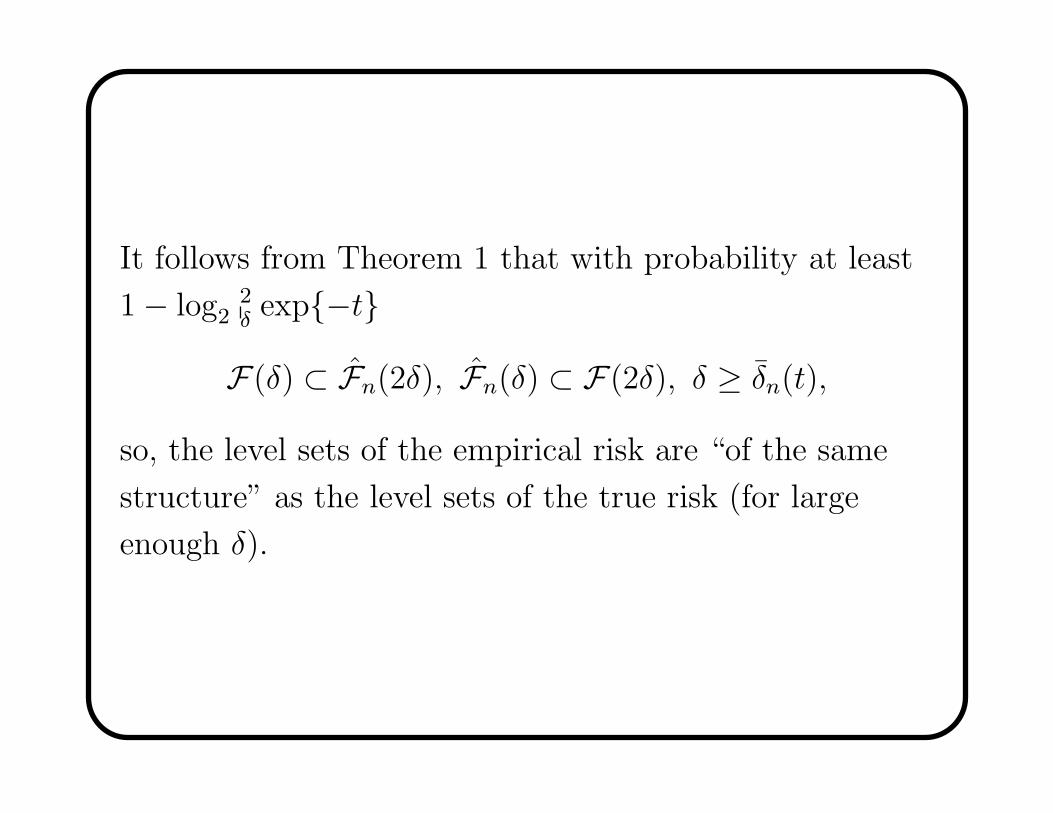
It follows from Theorem 1 that with probability at least

1 − log22δexp−t

F(δ) ⊂ Fn(2δ), Fn(δ) ⊂ F(2δ), δ ≥ δn(t),

so, the level sets of the empirical risk are “of the same

structure” as the level sets of the true risk (for large

enough δ).

Continuity Modulus of Empirical Processes

f ∗ := f ∗P := argminf∈FPf.

Expected local continuity modulus of empirical process:

ωn(δ) := ωn(F ; f ∗; δ) :=

E supP 1/2(f−f∗)2≤δ,f∈F

|(Pn − P )(f − f ∗)|.

A trivial bound: φn(δ) ≤ 2ωn(D(δ)).

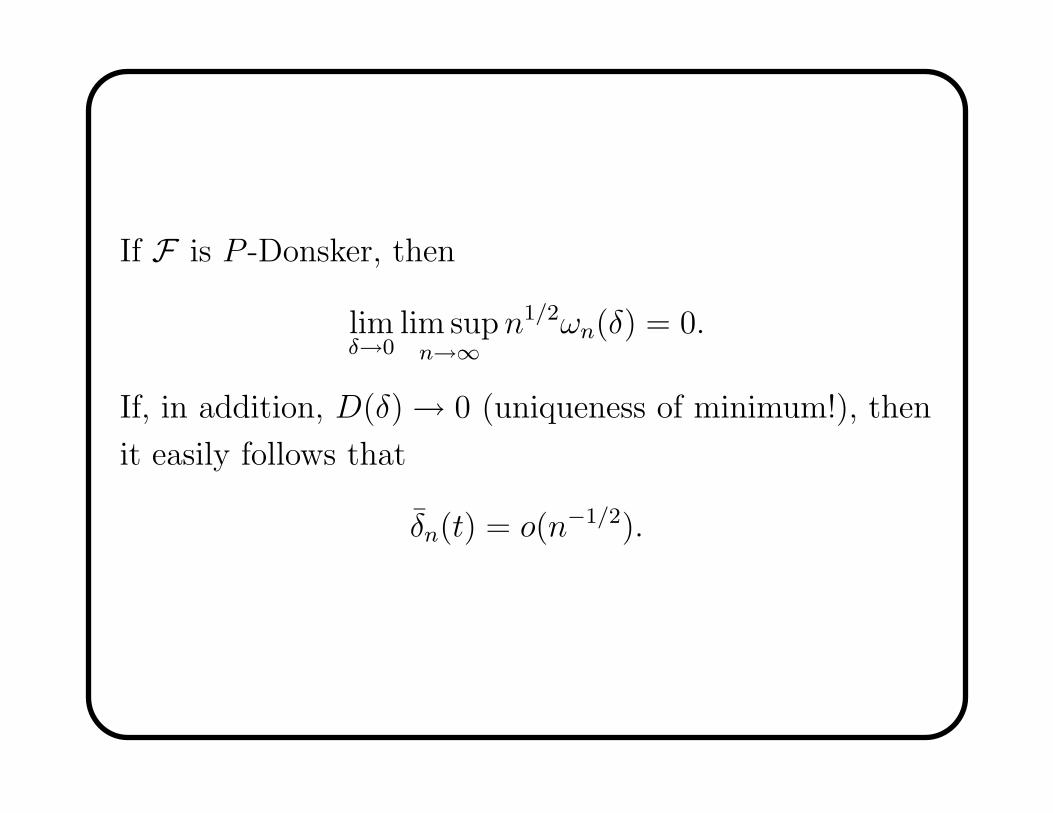
If F is P -Donsker, then

limδ→0

lim supn→∞

n1/2ωn(δ) = 0.

If, in addition, D(δ) → 0 (uniqueness of minimum!), then

it easily follows that

δn(t) = o(n−1/2).

Moreover, suppose that for some ρ ∈ (0, 1) and κ ≥ 1

(i) ωn(F ; f ∗; δ) ≤ Cn−1/2δ1−ρ;

(ii) DP (F ; δ) ≤ Cδ12κ .

Then

δn(t) ≤ K

(

n− κ2κ+ρ−1 +

t

n

)

.

This family of convergence rates occurs frequently in

regression (κ = 1) and classification problems (arbitrary

κ ≥ 1, Mammen and Tsybakov (1999), Tsybakov (2004)).

Excess Risk Bounds: κ = 1.

Below we give several bounds on δn(t) in the case κ = 1

or

D(δ) ≤ Cδ1/2.

In this case

φn(δ) ≤ 2ωn(D(δ)) ≤ 2ωn(Cδ1/2).

Let

θn(δ) := ωn(δ1/2).

Then

δn(t) ≤ K

(

θ♯n(1) +

t

n

)

.

Bounds on θ♯n(1).

Example 1. Linear Dimension F ⊂ L, L a subspace

of L2(P ), dim(L) = d. Then

θ♯n(1) ≤ Cd

n.

Example 2. VC-dimension F is a VC-type class with

VC-dimension V. Then

θ♯n(1) ≤ CV log n

V

n.

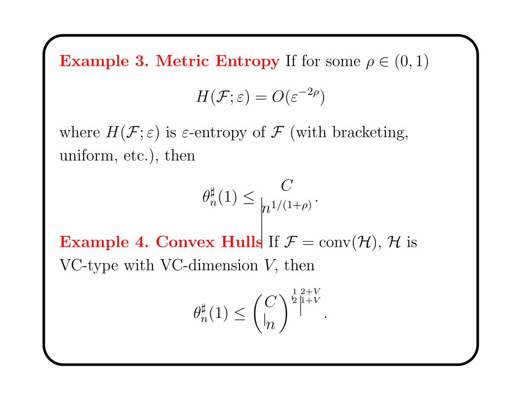
Example 3. Metric Entropy If for some ρ ∈ (0, 1)

H(F ; ε) = O(ε−2ρ)

where H(F ; ε) is ε-entropy of F (with bracketing,

uniform, etc.), then

θ♯n(1) ≤ C

n1/(1+ρ).

Example 4. Convex Hulls If F = conv(H), H is

VC-type with VC-dimension V, then

θ♯n(1) ≤

(

C

n

)12

2+V1+V

.

Example 5. Shattering Numbers If F is a class of

functions f : S 7→ 0, 1,

∆F(X1, . . . , Xn) :=

card

(

(f(X1), . . . , f(Xn)) : f ∈ F)

,

then

θ♯n(1) ≤ CE log ∆F(X1, . . . , Xn)

n.

Example 6 (Mendelson’s complexity). If K is a

symmetric nonnegatively definite kernel on S × S, HK is

the corresponding reproducing kernel Hilbert space and

F is the unit ball in HK , then

θ♯n(1) ≤ Cγ♯

n(1),

where

γn(δ) :=

(

n−1

∞∑

j=1

λj ∧ δ)1/2

,

λj are the eigenvalues of K.

L2-regression

(X,Y ) a random couple in S × [0, 1] with joint

distribution P.

Π the distribution of X.

g∗(x) := E(Y |X = x) the regression function.

f(x, y) := fg(x, y) := (y − g(x))2,

f ∗(x, y) := (y − g∗(x))2.

Then

Pf ∗ = minfPf = min

gE(Y − g(X))2.

For a class G of functions g : S 7→ [0, 1], let

F := fg : g ∈ G.

Let

gn := argming∈Gn−1

n∑

j=1

(Yj − g(Xj))2.

Then

fn = fgn = argminf∈FPnf.

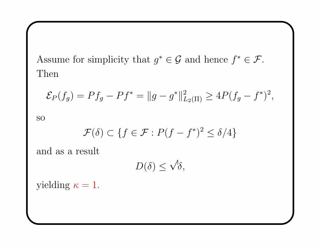
Assume for simplicity that g∗ ∈ G and hence f ∗ ∈ F .Then

EP (fg) = Pfg − Pf ∗ = ‖g − g∗‖2L2(Π) ≥ 4P (fg − f ∗)2,

so

F(δ) ⊂ f ∈ F : P (f − f ∗)2 ≤ δ/4and as a result

D(δ) ≤√δ,

yielding κ = 1.

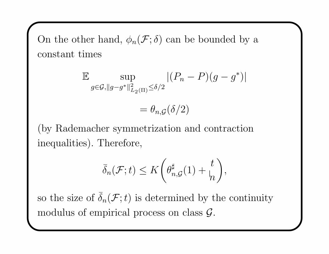
On the other hand, φn(F ; δ) can be bounded by a

constant times

E supg∈G,‖g−g∗‖2

L2(Π)≤δ/2

|(Pn − P )(g − g∗)|

= θn,G(δ/2)

(by Rademacher symmetrization and contraction

inequalities). Therefore,

δn(F ; t) ≤ K

(

θ♯n,G(1) +

t

n

)

,

so the size of δn(F ; t) is determined by the continuity

modulus of empirical process on class G.

This yields (with a minor further work), for instance, the

following result: for a convex class G and ‖ · ‖ = ‖ · ‖L2(Π)

P

‖gn − g∗‖2 ≥ infg∈G

‖g − g∗‖2+

K

(

θ♯n,G(1) +

t

n

)

≤ log2

2n

te−t.

If we do not assume that G is convex, then for all ε > 0

P

‖gn − g∗‖2 ≥ (1 + ε) infg∈G

‖g − g∗‖2+

K

(

θ♯n,G(ε) +

t

εn

)

≤ log2

2n

te−t.

Binary Classification

(X,Y ) is a random couple in S × 0, 1 with joint

distribution P ;

Π is the distribution of X;

The regression function:

η(x) := E(Y |X = x) = PY = 1|X = x.

A classifier: g : S 7→ 0, 1.The generalization error:

PY 6= g(X) = P(x, y) : y 6= g(x) = Πy 6= g(x).

Optimal Bayes classifier (that minimizes the

generalization error):

g∗(x) := g∗P (x) = I(η(x) ≥ 1/2).

The training error:

n−1

n∑

j=1

I(Yj 6= g(Xj)) = Pn(x, y) : y 6= g(x),

where (X1, Y1), . . . , (Xn, Yn) are i.i.d. copies of (X,Y ).

Let G be a class of binary classifiers such that g∗ ∈ G and

let gn be an empirical risk (training error) minimizer over

G. If

fg(x, y) := Iy 6=g(x)

and

F := fg : g ∈ G,then fg∗ is a minimizer of Pf and fgn is a minimizer of

Pnf over f ∈ F .

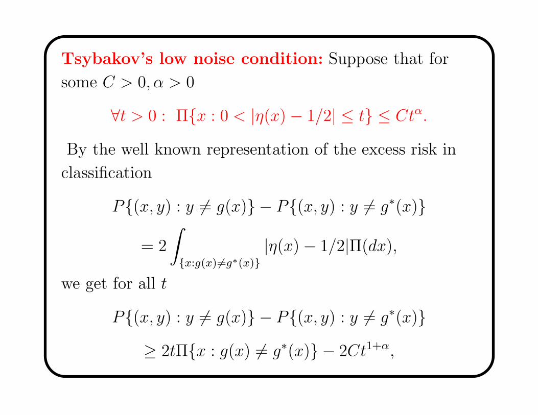
Tsybakov’s low noise condition: Suppose that for

some C > 0, α > 0

∀t > 0 : Πx : 0 < |η(x) − 1/2| ≤ t ≤ Ctα.

By the well known representation of the excess risk in

classification

P(x, y) : y 6= g(x) − P(x, y) : y 6= g∗(x)

= 2

∫

x:g(x) 6=g∗(x)

|η(x) − 1/2|Π(dx),

we get for all t

P(x, y) : y 6= g(x) − P(x, y) : y 6= g∗(x)

≥ 2tΠx : g(x) 6= g∗(x) − 2Ct1+α,

which by taking t of the order

Π1/αx : g(x) 6= g∗(x)

gives

P(x, y) : y 6= g(x) − P(x, y) : y 6= g∗(x)

≥ cΠκx : g(x) 6= g∗(x) = c‖fg − fg∗‖2κL2(Π)

with κ = (1 + α)/α > 1. Therefore

D(δ) ≤ Cδ12κ .

Given that the entropy of G is of the order O(ε−2ρ) for

some ρ < 1, our excess risk bounds give the convergence

rate O(n− κ2κ+ρ−1 ) discovered earlier by Mammen and

Tsybakov (1999), Tsybakov (2004). Alternatively, recall

that

∆G(X1, . . . , Xn) :=

card

(

(g(X1), . . . , g(Xn)) : g ∈ G)

.

then with probability at least 1 − log22nte−t

E(gn) ≤ δn(F ; t) ≤ C

[(

E log ∆G(X1, . . . , Xn)

n

)κ/(2κ−1)

+t

n

]

.

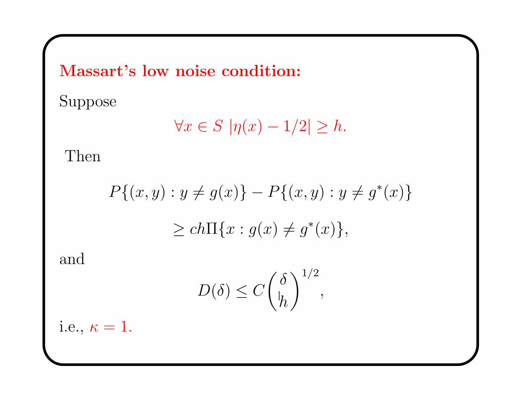
Massart’s low noise condition:

Suppose

∀x ∈ S |η(x) − 1/2| ≥ h.

Then

P(x, y) : y 6= g(x) − P(x, y) : y 6= g∗(x)

≥ chΠx : g(x) 6= g∗(x),and

D(δ) ≤ C

(

δ

h

)1/2

,

i.e., κ = 1.

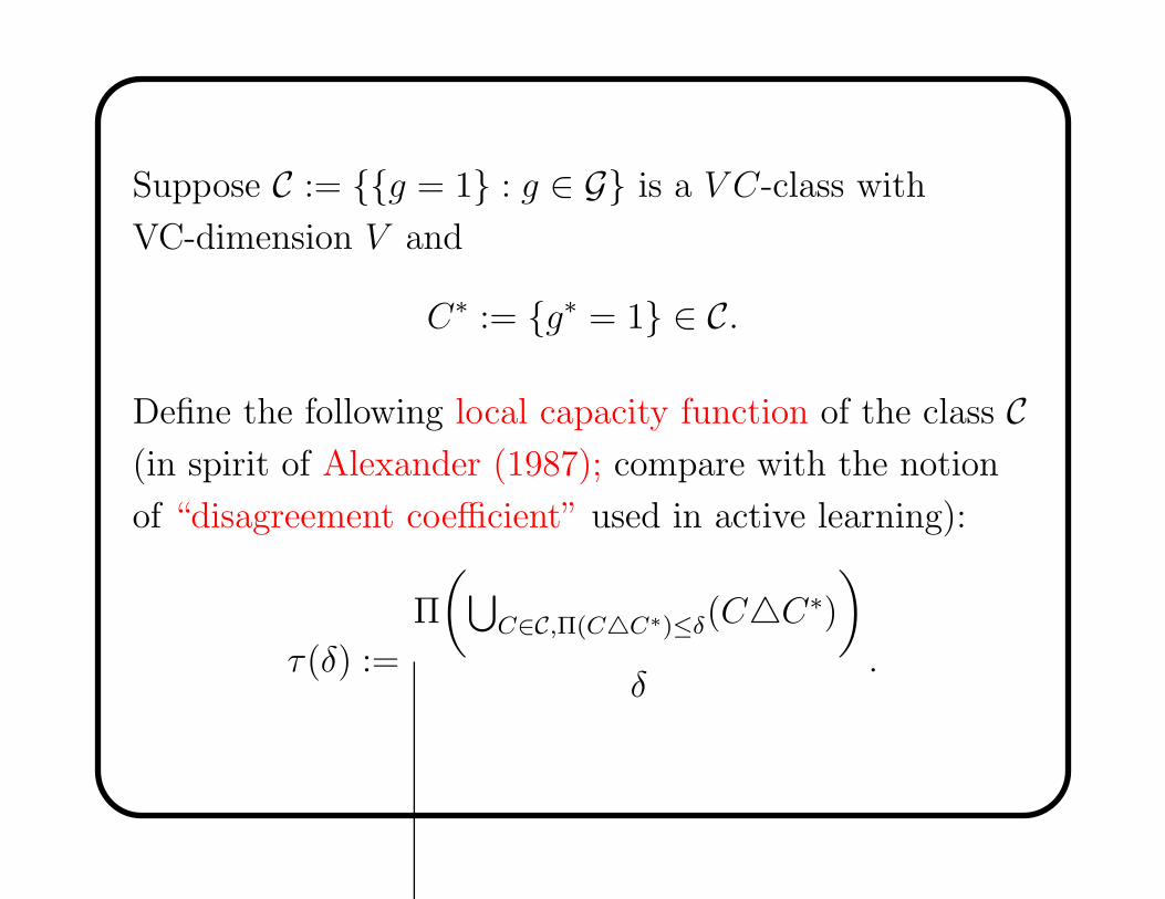
Suppose C := g = 1 : g ∈ G is a V C-class with

VC-dimension V and

C∗ := g∗ = 1 ∈ C.

Define the following local capacity function of the class C(in spirit of Alexander (1987); compare with the notion

of “disagreement coefficient” used in active learning):

τ(δ) :=

Π

(

⋃

C∈C,Π(CC∗)≤δ(CC∗)

)

δ.

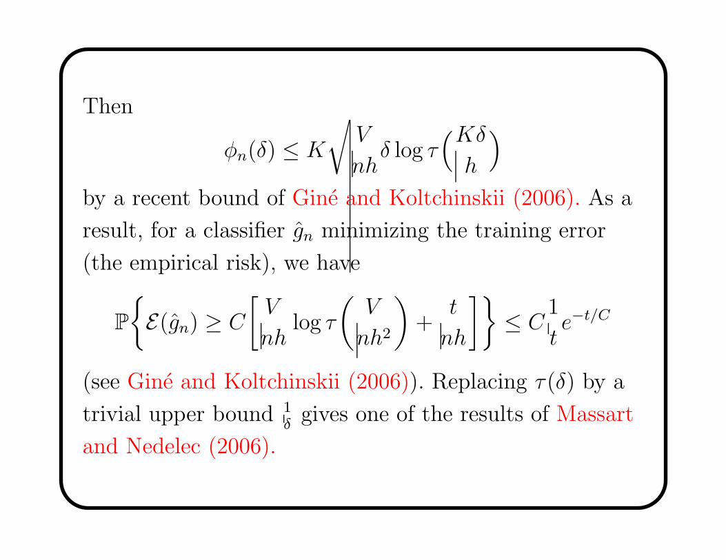
Then

φn(δ) ≤ K

√

V

nhδ log τ

(Kδ

h

)

by a recent bound of Gine and Koltchinskii (2006). As a

result, for a classifier gn minimizing the training error

(the empirical risk), we have

P

E(gn) ≥ C

[

V

nhlog τ

(

V

nh2

)

+t

nh

]

≤ C1

te−t/C

(see Gine and Koltchinskii (2006)). Replacing τ(δ) by a

trivial upper bound 1δ

gives one of the results of Massart

and Nedelec (2006).

Reminder:

Empirical excess risk:

En(f) := EPn(f) := Pnf − infFPnf ;

δ-minimal sets:

F(δ) := FP (δ) :=

f ∈ F : EP (f) ≤ δ

,

Fn(δ) := FPn(δ).

D(δ) := DP (δ) := supf,g∈F(δ)

(P (f − g)2)1/2

φn(δ) := E supf,g∈F(δ)

|(Pn − P )(f − g)|

Un(δ; t) := 2

(

φn(δ) +D(δ)

√

t

n+t

n

)

δn(t) := U ♯n,t(2

−1)

Data Dependent Excess Risk Bounds

Empirical versions of D and φn :

Dn(δ) := DPn(δ) := supf,g∈Fn(δ)

(Pn(f − g)2)1/2

and

φn(δ) := supf,g∈Fn(δ)

|Rn(f − g)|,

where Rn is the Rademacher process:

Rn(f) := n−1

n∑

i=1

εif(Xi), f ∈ F ,

εi being i.i.d. Rademacher random variables

independent of Xi.

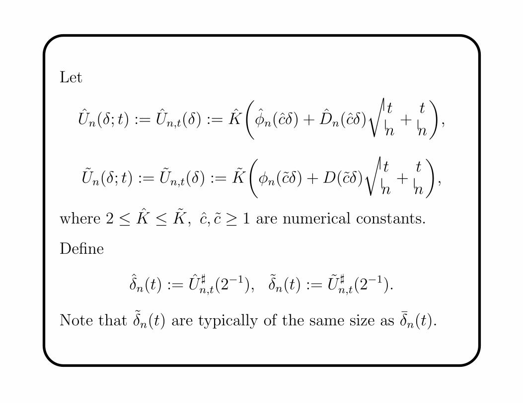
Let

Un(δ; t) := Un,t(δ) := K

(

φn(cδ) + Dn(cδ)

√

t

n+t

n

)

,

Un(δ; t) := Un,t(δ) := K

(

φn(cδ) +D(cδ)

√

t

n+t

n

)

,

where 2 ≤ K ≤ K, c, c ≥ 1 are numerical constants.

Define

δn(t) := U ♯n,t(2

−1), δn(t) := U ♯n,t(2

−1).

Note that δn(t) are typically of the same size as δn(t).

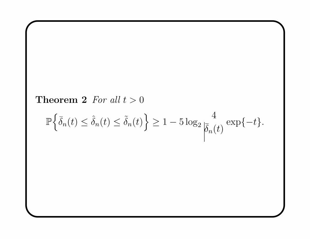
Theorem 2 For all t > 0

P

δn(t) ≤ δn(t) ≤ δn(t)

≥ 1 − 5 log2

4

δn(t)exp−t.

Model Selection

References:

Vapnik and Chervonenkis, Structural Risk Minimization

(70s-80s)

Birge and Massart (1997)

Barron, Birge and Massart (1999)

Massart (2000, 2007)

Koltchinskii (2001, 2006, 2008)

Lugosi and Wegkamp (2004)

Blanchard, Lugosi and Vayatis (2003)

Blanchard, Bousquet and Massart (2008)

Model Selection Framework

• A family (a ”sieve”)

F1,F2, · · · ⊂ F

of function classes approximating F ;

• A sequence fn,k of empirical risk minimizers:

fn,k := argminf∈FkPnf.

Goal of Model Selection: to construct

k = k(X1, . . . , Xn)

such that f = fn,k ∈ F has a ”nearly optimal” global

excess risk

E(F ; f) = P f − inff∈F

Pf.

More precisely, suppose that for some (unknown) k∗ ∈ N

f ∗ = argminf∈FPf ∈ Fk∗ .

Then the goal is to find a data dependent k ∈ N such

that with a high probability

EP (F ; f) ≤ Cδn(Fk∗).

More generally,

EP (F ; f) ≤ C infk∈N

[

inff∈Fk

Pf − Pf ∗ + πn(k)]

for some ”ideal” penalties πn(k) (roughly, of the size of

δn(Fk) = δn(Fk; tk)).

The bounds of this type are often called oracle

inequalities.

Ideal solution: find k by minimizing the global excess

risk EP (F ; fn,k) over k ∈ N.

It is impossible since the global excess risk is distribution

dependent. We need tight data-dependent bounds on

EP (F ; fn,k).

The following representation of the global excess risk

(“bias-variance decomposition”) is trivial

EP (F ; fn,k) = infFk

Pf − Pf∗ + EP (Fk; fn,k).

It shows that part of the problem is to find a

data-dependent bound δn(Fk) on the local excess risk

(the random error)

EP (Fk; fn,k).

Another part, is to bound the approximation error

infFk

Pf − Pf ∗

in terms of its empirical version infFkPnf − Pnf

∗ in order

to develop a penalization approach to model selection.

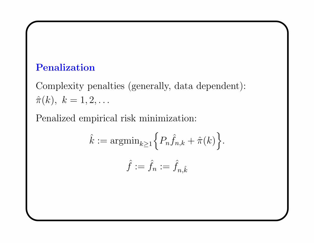
Penalization

Complexity penalties (generally, data dependent):

π(k), k = 1, 2, . . .

Penalized empirical risk minimization:

k := argmink≥1

Pnfn,k + π(k)

.

f := fn := fn,k

Monotone Families

Fk ⊂ Fk+1, k ≥ 1

Design of Penalties

πn(k) = 4δn(k) := 4δn(Fk; tk)

k := argmink≥1

Pnfn,k + 4δn(k)

.

f := fn,k.

Oracle Inequality

Theorem 3 (Bartlett) For any sequence tk of positive

numbers,

P

EP (F ; f) ≥ infk≥1

inff∈Fk

Pf − inff∈F

Pf + 9δn(k)

≤ 5∞

∑

k=1

log2

4n

tke−tk ,

where δn(k) := δn(Fk; tk).

General Families

Let f∗ := argminf∈FPf.

ϕ convex nondecreasing function on [0,+∞), ϕ(0) = 0,

ϕ(uv) ≤ ϕ(u)ϕ(v), u, v ≥ 0

(example: ϕ(u) = u2).

Basic Assumption: Excess Risk - Variance Link

∀f ∈ F : Pf − Pf∗ ≥ ϕ

(

√

VarP (f − f∗)

)

.

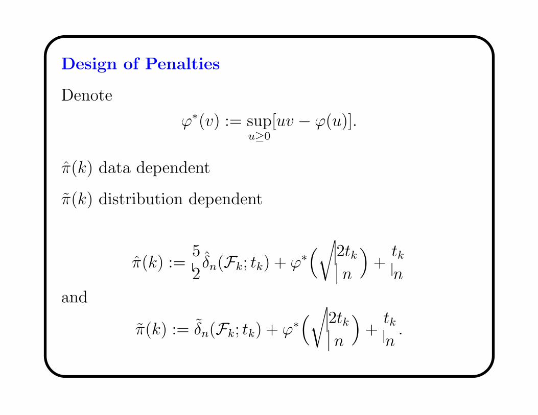
Design of Penalties

Denote

ϕ∗(v) := supu≥0

[uv − ϕ(u)].

π(k) data dependent

π(k) distribution dependent

π(k) :=5

2δn(Fk; tk) + ϕ∗

(

√

2tkn

)

+tkn

and

π(k) := δn(Fk; tk) + ϕ∗(

√

2tkn

)

+tkn.

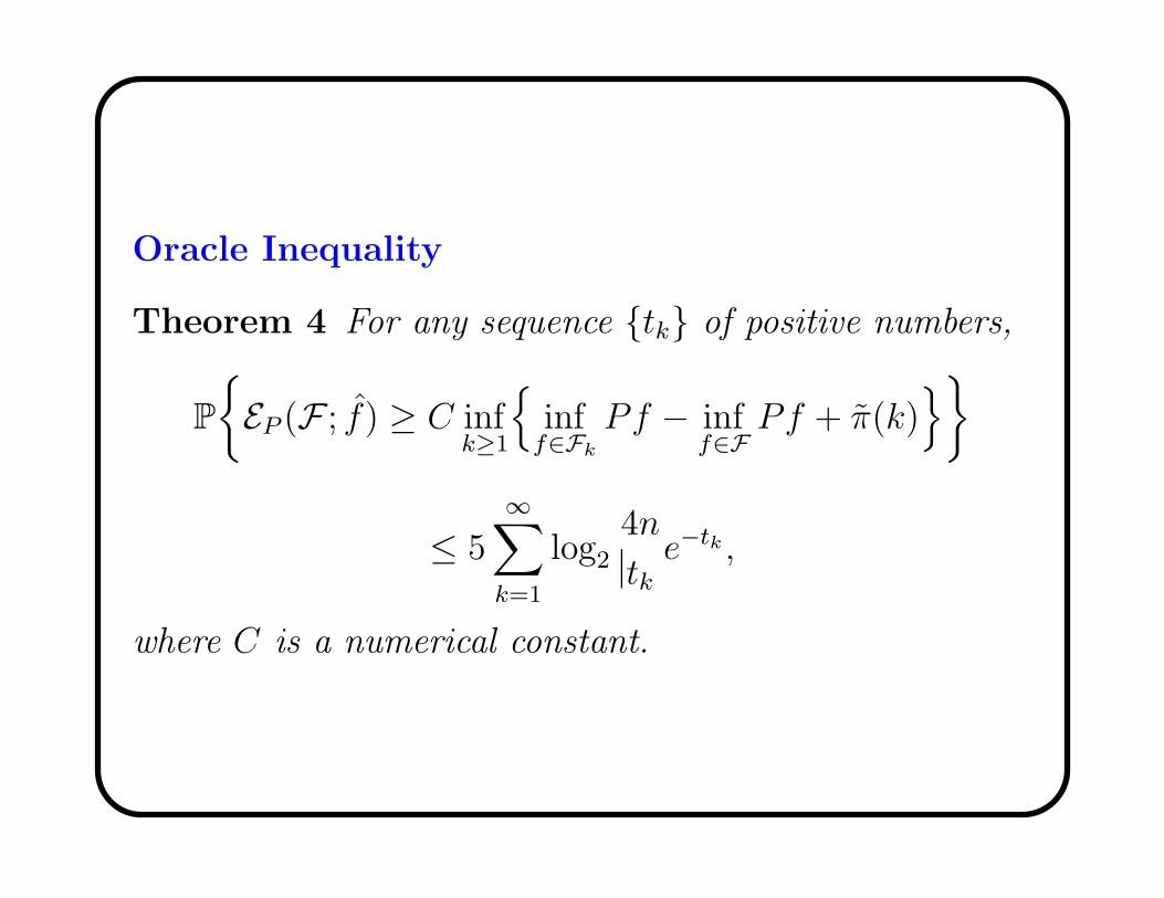
Oracle Inequality

Theorem 4 For any sequence tk of positive numbers,

P

EP (F ; f) ≥ C infk≥1

inff∈Fk

Pf − inff∈F

Pf + π(k)

≤ 5∞

∑

k=1

log2

4n

tke−tk ,

where C is a numerical constant.

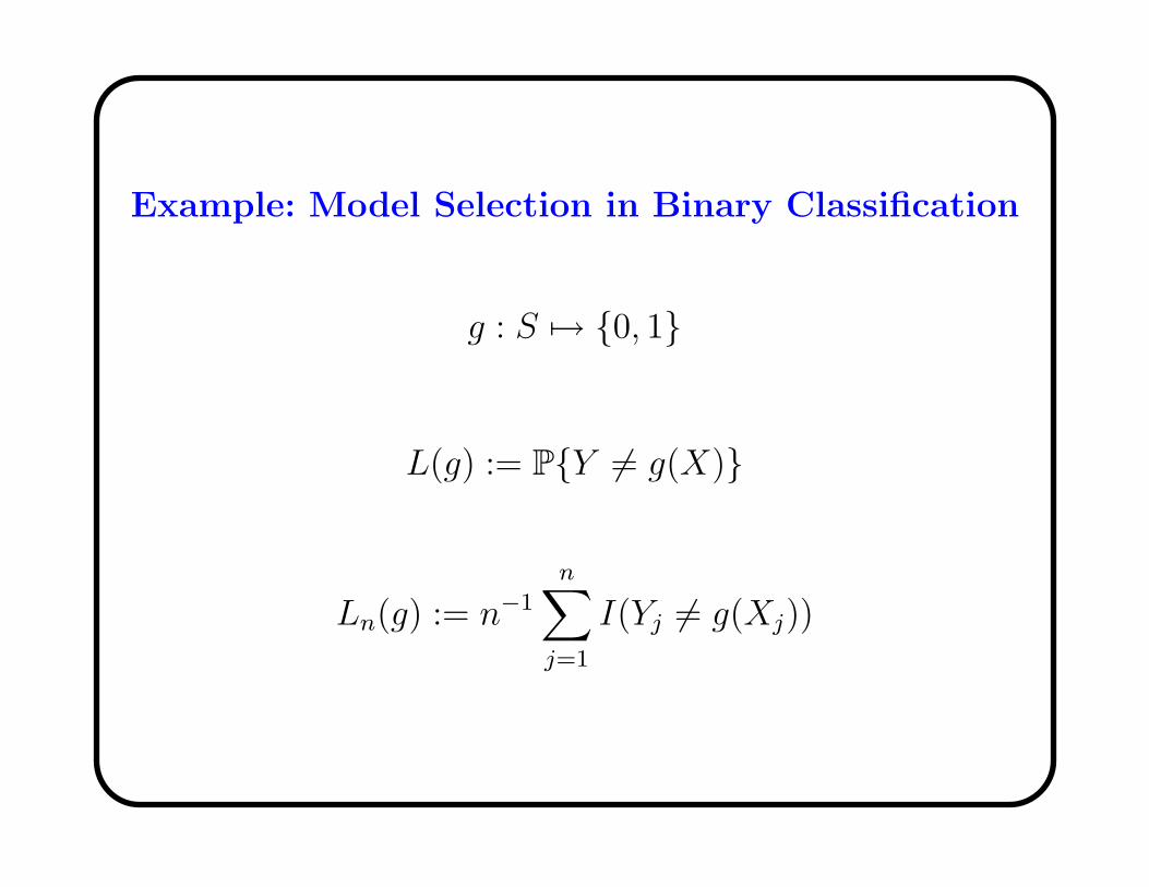
Example: Model Selection in Binary Classification

g : S 7→ 0, 1

L(g) := PY 6= g(X)

Ln(g) := n−1

n∑

j=1

I(Yj 6= g(Xj))

Regression Function

η(x) := E(Y |X = x)

Bayes Classifier

g∗(x) = I(η(x) ≥ 1/2)

Massart’s low noise condition:

Suppose

∀x ∈ S |η(x) − 1/2| ≥ h > 0,

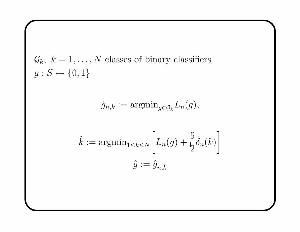
Gk, k = 1, . . . , N classes of binary classifiers

g : S 7→ 0, 1

gn,k := argming∈GkLn(g),

k := argmin1≤k≤N

[

Ln(g) +5

2δn(k)

]

g := gn,k

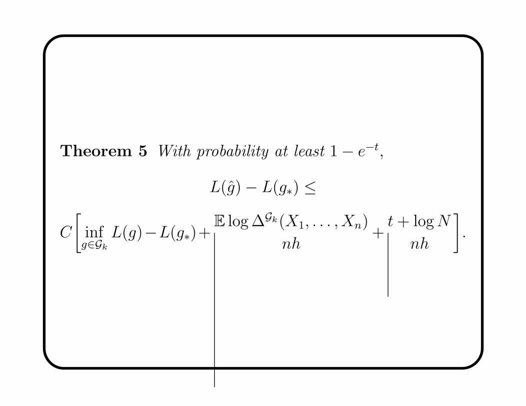
Theorem 5 With probability at least 1 − e−t,

L(g) − L(g∗) ≤

C

[

infg∈Gk

L(g)−L(g∗)+E log ∆Gk(X1, . . . , Xn)

nh+t+ logN

nh

]

.