The delay of open Markovian queueingnetworks: Uniform functional bounds, heavy

tra�c pole multiplicities, and stability�y

C. Humes, Jr.,zJ. Ouxand P. R. Kumar{

AbstractFor open Markovian queueing networks, we study the functional dependence of themean number in the system (and thus also the mean delay since it is proportional toit by Little's Theorem) on the arrival rate or load factor. We obtain linear programs(LPs) which provide bounds on the pole multiplicity M of the mean number in thesystem, and automatically obtain lower and upper bounds on the coe�cients fCig of

the expansion �CM(1��)M + �CM�1(1��)M�1 + � � �+ �C1(1��) + �C0, where � is the load factor, whichare valid for all � 2 [0; 1). Our LPs can thus establish the stability of open network-s for all arrival rates within capacity, while providing uniformly bounding functionalexpansions for the mean delay, valid for all arrival rates in the capacity region. Thecoe�cients fCig can be optimized to provide the best bound at any desired value ofthe load factor, while still maintaining its validity for all � 2 [0; 1). While the aboveLPs feature L(L+1)(M+1)2 variables where L is the number of bu�ers in the network,for balanced systems we further provide a lower dimensional LP featuring just S(S+1)2variables, where S is the number of stations in the network. This bound asymptoticallydominates in heavy tra�c a bound obtainable from the Pollaczek-Khintchine formula,and can capture interactions between multiple bottleneck stations in heavy tra�c. We

�Please address all correspondence to the third author.yThe research reported here has been supported by the U.S. Army Research O�ce under Contract No.DAAH-04-95-1-0090, the National Science Foundation under Grant No. ECS-94-03571, the Joint ServicesElectronics Program under Contract No. N00014-90-J-1270, FAPESP grants 93/0603-1 and 94/1376-1, andby CNPq and IBM-Brasil.zDepartamento de Ciencia da Computacao, Instituto de Mathematica e Estatistica, University of SaoPaulo, Brazil. This work was done while the author was visiting the University of Illinois.xDepartment of Decision Sciences, Faculty of Business Administration, National University of Singapore,Singapore 0511. This work was done while the author was visiting the University of Illinois.{Department of Electrical and Computer Engineering, and the Coordinated Science Laboratory, Univer-sity of Illinois, 1308 West Main St., Urbana, IL 61801.1

also provide an explicit upper bound for all scheduling policies in acyclic networks, andfor the FBFS policy in open re-entrant lines.Key Words: Queueing networks, open networks, performance evaluation, schedul-ing policies, delay, stability, heavy tra�c behavior.

1 IntroductionWe address the problem of determining the delay of open Markovian queueing networks asa function of the arrival rate. A queueing network is open if customers arrive to the systemfrom the outside and eventually depart. It is said to be Markovian if it has Bernoulli routing,and service and interarrival times are exponentially distributed.

For such networks, the mean delay Du(�) under a scheduling policy u depends on thearrival rate � of customers from the outside. If the mean delay Du(�) is �nite, we say thatthe system is stable under the scheduling policy u at the arrival rate �. Let �� denote thesupremal arrival rate that the system is stable, if properly scheduled. Given a particularvalue of � < ��, we have provided in Kumar and Meyn (1995) a linear program (LP) that canestablish stability at that speci�c value � of the arrival rate. Also, LPs have been providedin Kumar and Kumar (1994) and Bertsimas, Paschalidis and Tsitsiklis (1994) that provideupper and lower bounds on the mean delay, again for speci�c values of �. In Kumar andMeyn (1996) we have shown that the LPs for stability and performance are the duals of eachother.

The above results however only provide bounds on the performance, pointwise for eachspeci�c value � of the arrival rate, or stability pointwise at each speci�c value of �. In thispaper, our objective is to establish the behavior of networks over all �'s. We study thefunctional dependence of Du(�) on � for all arrival rates 0 � � < ��. If a system is stablefor all � in [0; ��) for a particular scheduling policy u, we say that u is stable throughout thecapacity region. After stability, we are interested in how the delay Du(�) varies with � in

2

[0; ��). If f(�) � Du(�) � g(�) for all 0 � � < ��, then we call f and g lower and upperfunctional bounds on Du, respectively. Of particular interest is the behavior of the delay inheavy tra�c as �% ��. If Du(�) = CM+o(1)(����)M , where CM > 0, then we say that M is the polemultiplicity of the delay in heavy tra�c, and CM is the growth constant.

We obtain LPs which provide bounds on the pole multiplicity M , and automaticallyobtain lower and upper bounds on the coe�cients fCig of the functional expansion �CM(1��)M +�CM�1(1��)M�1+� � �+ �C1(1��)+�C0 for the mean number in the system. Above, � := ��� is the nominal

load on the network. By this approach, we obtain an LP test that establishes stabilitythroughout the capacity region 0 � � < 1, and simultaneously obtains uniformly boundingfunctional expansions valid throughout the capacity region. The functional bound can beoptimized to provide the best bound at any particular value of �, while still maintaining itsuniform validity for all � 2 [0; 1). All results in this paper will be furnished in terms of themean number in the system, and are easily translated by Little's Theorem into correspondingresults concerning the mean delay by simply multiplying by ��1.

Our results develop lower bounds valid either for the class of all scheduling policies, or fora particular bu�er priority policy. Our upper bounds are developed either for the class of allnon-idling scheduling policies (since allowing idling allows in�nite delay), or for a particularbu�er priority policy.

For balanced networks where all stations are equally loaded, we further obtain a reduceddimensional LP, for a functional lower bound on the delay, consisting of just S(S+1)2 variablesrather than the L(L+1)(M+1)2 variables for the LPs mentioned above. Here S is the number ofstations in the networks. In many applications it is far smaller than L, the number of bu�ersin the network. We show that for re-entrant lines this functional bound asymptoticallydominates in heavy tra�c a lower bound that can be derived from the Pollaczek-Khintchineformula, and that it can capture nontrivial interactions between multiple bottleneck stationsin heavy tra�c.

3

We also study the possibility of obtaining upper bounds through our LP approach forall systems and scheduling policies known to be stable throughout the capacity region. Weobtain explicit upper bounds on the mean delay of all non-idling scheduling policies in acyclicnetworks, and the mean delay of the First Bu�er First Serve (FBFS) bu�er priority policyfor open re-entrant lines. We also show that our approach cannot establish the stability ofthe Last Bu�er First Serve (LBFS) policy.

By providing uniformly bounding functional expansions of the form �CM(1��)M + �CM�1(1��)M�1 +� � �+ �C1(1��) +�C0, valid for all arrival rates, which are obtained merely by solving LPs for thecoe�cients, these procedures can provide useful information with little computational e�ortfor non-product form networks previously considered intractable.

Another value of our results is that they allow us to better comprehend what the linearprogramming approach to stability and performance is really providing us. In all examplesstudied by us, the functional bounds yield the same heavy tra�c growth constant CM asthe pointwise bounds do numerically. Thus, through studying the closed form expressionsprovided by the functional bounds, we are able to assess the quality of the original pointwisebounds themselves.

The issue of bounding functional expansions seems to be relatively unexplored, though itis quite interesting for applications. We are not aware of prior work in this area. For singleserver queues, Gong and Hu (1992) [5] have studied Maclaurin series solutions of Lindley'sequations. Girish and Hu (1995) have investigated tandem queues by this procedure. Gongand Yang (1995) have also investigated the problem of extrapolating the performance curvefrom a known set of explicit points on it via Pade approximations.

Our speci�c results are as follows:

(i) We obtain LPs which establish stability throughout the capacity region, provide lowerand upper bounds on pole multiplicity, and provide uniformly bounding functional

4

expansions for the mean delay that can be tailored for best �t at any particular loadinglevel (Theorems 3, 4 and 5).

(ii) We provide a reduced dimensional reduced LP which gives a functional lower bound onthe delay of all scheduling policies for balanced systems (Theorem 6). We show thatfor re-entrant lines this bound asymptotically dominates in heavy tra�c a bound thatcan be derived from the Pollaczek-Khintchine formula (Theorem 7), and that it cancapture multiple bottleneck interactions in heavy tra�c (Example 4).

(iii) We provide an explicit upper bound on the delay of the FBFS policy (Theorems 8 and9).

(iv) We provide an explicit upper bound on the delay for all acyclic networks (Theorem 10).

The rest of this paper is organized as follows. In Section 2 we begin with a review ofthe pointwise bounds for each �xed value of �. In Section 3, we sow the seed of the ideafor obtaining functional expansions. In Section 4, we investigate the feasible solutions of thedual LPs, exhibiting a key fundamental identity and a key inequality. In Section 5 we providethe uniformly bounding functional expansions and LPs for their coe�cients. In Section 6,we provide a reduced dimensional LP for the functional lower bound for balanced systems,and in Section 7 we show that for re-entrant lines this bound asymptotically dominates inheavy tra�c a bound that can be derived from the Pollaczek-Khintchine formula, and thatit can capture nontrivial interactions between multiple bottleneck stations in heavy tra�c.In Section 8 we turn to upper bounds, and in Sections 9 and 10 we obtain the upper boundsfor the FBFS policy, and for all acyclic networks, respectively.

5

λ

Station 1=σ(1)=σ(3)

Station 2=σ(2)=σ(4)

µ1

µ3

µ2

µ4

b1 b2

b4b3

p12

p14

p∗1

p∗2

p23

p2∗

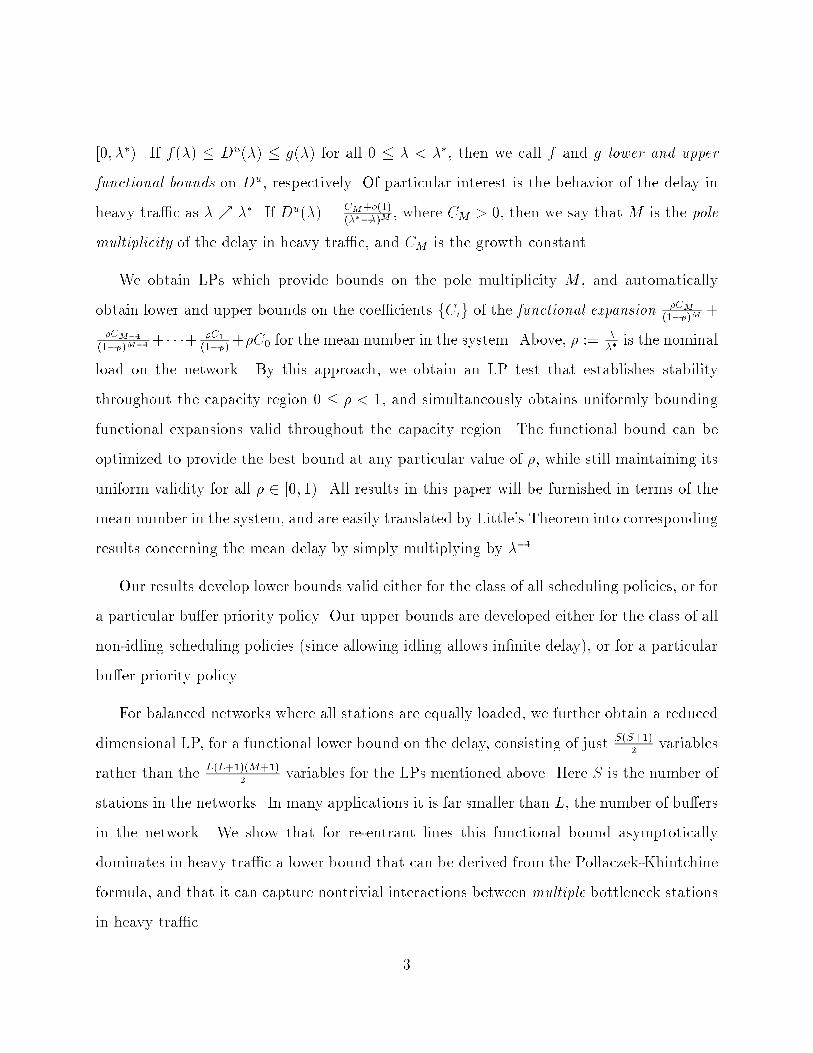
2 Pointwise bounds for a �xed arrival rateWe shall carry out our development on the following model of a Markovian queueing network;see Figure 1. There are S stations labeled f1; 2; . . . ; Sg, and L bu�ers labeled fb1; b2; . . . ; bLg.Bu�er bi is served by station �(i) 2 f1; 2; . . . ; Sg. Customers arrive to the system as a Poissonprocess of rate �. Upon arrival they join bu�er bi with probability p�i. Customers in bu�erbi require an exponentially distributed service time with mean 1=�i from station �(i). Aftercompleting service at bi, they move to bu�er bj with probability pij, or leave the system withprobability pi�. We call such a system an open Markovian queueing network.

Figure 1: An open Markovian queueing network.

Let wi(t) := 1 if station �(i) is busy serving a customer in bi at time t; and := 0otherwise. We denote the number of customers in bu�er bi at time t by xi(t), and byx(t) = (x1(t); x2(t); . . . ; xL(t))T the corresponding vector. We assume that all stochasticprocesses are right continuous with left limits.

We convert this system to discrete time by the method of uniformization, see Lipp-man (1975). We normalize time so that � +Pi �i = 1. Then we suppose that every bu�erhas either a real or virtual customer in service, and sample the system at the sequence f�ng

6

of random times which consists of all arrival times, real service completion times, and virtualservice completion times. We denote x(�n) and w(�n) by x(n) and w(n), for brevity.

Throughout we assume that the scheduling policy employed is non-idling, i.e., a stationcannot stay idle if there is work for it. (The lower bound for the class of all non-idlingpolicies also applies to the class of all scheduling policies, as noted in the proof of Theorem 5.)Quantitatively, the property of non-idling can be expressed as xi(n) � 1) Pj2�(i)wj(n) = 1,where, by \j 2 �" we mean fj : �(j) = �g. A consequence of this is,

xi(n) = Xj2�(i)wj(n)xi(n): (1)

In addition, one always hasxi(n) �X

j2�wj(n)xi(n) for all �: (2)

On occasion, in the sequel, we will consider bu�er priority policies. These are de�nedby a bu�er priority ordering � = (�(1); . . . ; �(L)) which is a permutation of f1; 2; . . . ; Lg. Ifbu�ers bi and bj share the same station, i.e., �(i) = �(j), then priority is given to bj over biif �(j) < �(i). The priority discipline is preemptive resume. As a consequence,

wi(n)xj(n) = 0 if �(i) = �(j) and �(j) < �(i): (3)

Consider now a scheduling policy that is stationary, i.e., wi(t) depends only on x(t),and non-idling. If the resulting system is stable with a �nite second moment for x(n) insteady-state, then

E[E[xT (n+ 1)Qx(n+ 1)jFn]� xT (n)Qx(n)] = 0 in steady state;where Fn is the past �-algebra. De�ne the steady state expectations,

zij := E[wi(n)xj(n)]; (4)�xi := E(xi(n)): (5)

7

It has been shown in Kumar and Kumar (1994) and Bertsimas, Paschalidis and Tsitsiklis(1994) that by taking Q = eieTj + ejeTi , where ei = (0; . . . ; 0; 1; 0; . . . ; 0)T with a 1 in the ithplace, one obtains the following set of equalities:

2�p�i�xi � 2�izii(1� pii) + 2Xj 6=i�jpjizji + 2�i�i(1� pii) = 0 for i = 1; 2; . . . ; L; (6)�(p�i�xj + p�j�xi)� �i(pij�i + zij)� �j(pji�j + zji)+Xk �k(pkizkj + pkjzki) = 0 for all 1 � i < j � L: (7)

Above, the �i's are the unique solution of the following tra�c equations,�p�i +

LXk=1�kpki�k = �i�i; for i = 1; 2; . . . ; L: (8)

Note that �i is the nominal load on station �(i) due to bu�er bi. It varies linearly with �.Using (4,5), one can rewrite (1, 2, 3) as,

�xi = Xj2�(i) zji for 1 � i � L; (9)

�xi � Xj2� zji for 1 � i � L and all �; (10)

zij = 0 if �(i) = �(j) and �(j) < �(i): (11)

It is shown in Kumar and Meyn (1996) that (6,7) are valid even if one only assumes�niteness of the �rst moment. There, by using some properties of the class of all non-idling policies, we have established the following Linear Program (LP) bounds, without evenassuming �niteness of the �rst moment. They provide bounds, pointwise for each speci�cvalue of �, and so we call them the pointwise bound LPs.Theorem 1. The pointwise bound LPs. Under any stationary non-idling schedulingpolicy, the mean number of customers in the system is bounded above by

Max LXi=1 �xi; (12)

8

subject to the constraints (6, 7, 9, 10), and�xi � 0; zij � 0 for 1 � i; j � L: (13)

The mean number of customers is bounded below byMin LX

i=1 �xi; (14)subject to the same constraints (6, 7, 9, 10, 13).

For bu�er priority policies, the upper bound is valid only under a �nite �rst momentassumption.Theorem 2. Pointwise bound LPs for bu�er priority policies. Consider a bu�erpriority policy �.

(i) The mean number of customers in steady state is bounded below by (14), subject to theconstraints (6, 7, 9, 10, 13) and the bu�er priority constraints (11).

(ii) If the mean number of customers in steady-state is �nite, then it is bounded above by(12), subject to the same constraints (6, 7, 9, 10, 13, 11).

3 Primal expansionsThe above results provide LPs for obtaining pointwise bounds on the mean number in thesystem (or equivalently mean delay, through Little's Theorem) for each �xed value of thearrival rate �. Our goal however is to study the functional dependence of the mean delay onthe arrival rate �.

Denote the nominal load on station � by�� :=X

i2� �i;

9

and the nominal load on the system, or more precisely on a bottleneck station, by� := Max���:

Both depend linearly on �. The tra�c capacity of the system is�� := supf� : Max��� < 1g:

Let ��i and ��� denote the limiting values of �i and �� when the arrival rate �% ��.To make explicit the dependence on the loading � (or equivalently the arrival rate �),

we will denote by zij(�) and �xi(�) the expectations de�ned in (4; 5) when the arrival rate is� = ���.

We commence the development of functional dependence by examining the consequencesof a truncated Laurent series type expansion for zij(�). While this expansion itself may notbe valid, we will later establish the implied results rigorously.Truncated Laurent Series Condition (TLS)For some M � 1, and constants z(0)ij ; z(1)ij ; . . . ; z(M)ij ,

zij(�) = z(M)ij(1� �)M + z(M�1)ij(1� �)M�1 + � � �++z(0)ij +O(1� �) for 0 � � < 1: (15)

Trivially, from (9), it follows that we must then have

�xi(�) = �x(M)i(1� �)M + �x(M�1)i(1� �)M�1 + � � �+ �x0i +O(1� �); where (16)�x(m)i = X

j2�(i) z(m)ji : (17)

The following Lemma shows how to obtain the equality constraints satis�ed by the coe�-cients fz(m)ij ; �x(m)i g of the above expansions.Lemma 1. Suppose a vector y(�) satis�es

10

(i) y(�) = PMm=0 y(m)(1��) +O(1� �) in 0 � � < 1,(ii) �Ay(�) +By(�) = c.

Then the fy(m)g satisfy the following equations:(A+B)y(0) � Ay(1) = c; (18)

(A+B)y(m) � Ay(m+1) = 0 for 1 � m �M � 1; (19)(A+B)y(M) = 0: (20)

Proof. The results follow by writing � = 1� (1� �), and matching coe�cients of powersof (1� �).

From this one obtains the following constraints for fz(m)ij g.Lemma 2. Under Condition (TLS), fz(m)ij ; �x(m)i g satisfy the following for 0 � m �M :

2��p�i�x(m)i � 1(m �M � 1)2��p�i�x(m+1)i � 2�iz(m)ii (1� pii)+2Pj 6=i �jpjiz(m)ji + 1(m = 0)2�i��i (1� pii) = 0; (21)

��p�i�x(m)j � 1(m �M � 1)��p�i�x(m+1)j + ��p�j�x(m)j � 1(m �M � 1)��p�j�x(m+1)j�1(m = 0)�ipij��i � �iz(m)ij � 1(m = 0)�jpji��j � �jz(m)ji (22)

+Xk �k(pkiz(m)kj + pkjz(m)ki ) = 0 for j � i+ 1:

Proof. The result is obtained by applying Lemma 1 to the constraints of the LP of Theo-rem 1. Noting � = ��� and �i = ���i , equation (6) can be written as

�[2����ixi(�) + 2�i��i (1� pii)] + [�2�i(1� pii)zii(�) + 2Xj 6=i �jpjizji(�)] = 0: (23)

11

De�ne the vectors y(�) := (z1i; z2i; . . . ; zLi; xi; 1)T , A := (0; . . . ; 0; 2��p�i; 2�i��i (1� pii)), andB := (B1; . . . ; BL; 0; 0) with Bj := 2�jpji for j 6= i, Bi := �2�i(1 � pii). Then (23) can bewritten as �Ay(�) + By(�) = 0. The equation (21) then follows from Lemma 1. Similarly(22) can be obtained.

This suggests the possibility of directly bounding the coe�cients fz(m)ij ; �x(m)i g, and thusobtaining uniformly bounding functional expansions for the performance. One is thus ledto consider the following LP, which we shall call the LP for the uniformly upper boundingfunctional expansion:

Max LXi=1 �x

(M)isubject to the constraints (21, 22, 17) and

�x(m)i � Xj2� z

(m)ji ; (24)�x(m)i � 0: (25)

(For m 6=M , the constraints (24,25) are not forced by the Condition (TLS)).One hopes that if f�x(m)i g is an optimal solution, then an uniformly upper bounding

functional expansion of the following form is valid for all 0 � � < ��,Ejx(n)j � LX

i=1�x(M)i(1� �)M + LX

i=1�x(M�1)i(1� �)M�1 + . . . + LX

i=1 �x(0)i +O(1� �); where jxj := LX

i=1 xi:

However, all this is heavily contingent on the unjusti�ed use of Condition (TLS). In fact,we have not even established stability of the system for all � 2 [0; ��). Moreover, there isthe issue of what is the appropriate value of M to choose. To resolve these issues and thusrigorously obtain functional bounds, we turn to the duals of the above LPs.

12

4 The fundamental identity and inequalityIn Kumar and Meyn (1996) we have shown how to obtain Lyapunov functions that possessnegative drift and thus establish stability, by taking the dual of the pointwise upper boundLP. Here we will employ duality in a di�erent way to actually give a uniformly boundingfunctional expansion for the performance.

Associating the dual variables (�12q(m)ii ) with (21), and (�q(m)ij ) with (22), yields thefollowing duals of the pointwise upper and lower bound LPs:Dual of the LP for the uniformly upper bounding functional expansion

Min LXi=1 �i�

�i (q(0)ii �Xj pijq(0)ij ) (26)subject to:

��PLi=1 p�i�q(m)ij � 1(m � 1)q(m�1)ij �+Maxi2�(j)�i

Xk pikq(m)kj � q(m)ij

!

+P� 6=�(j)Maxi2��i X

k pikq(m)kj � q(m)ij!+

� �1(m =M) for 1 � j � L and m �M:(27)

Dual of the LP for the uniformly lower bounding functional expansionMax LX

i=1 �i��i (�q(0)ii +X

j pijq(0)ij ) (28)subject to:

��PLi=1 p�i�q(m)ij � 1(m � 1)q(m�1)ij �+Maxi2�(j)�i

Xk pikq(m)kj � q(m)ij

!

+P� 6=�(j)Maxi2��i X

k pikq(m)kj � q(m)ij!+

� 1(m =M) for 1 � j � L and m �M: (29)

The key to exploiting the properties of feasible solutions of these LPs is the followingfundamental identity.

13

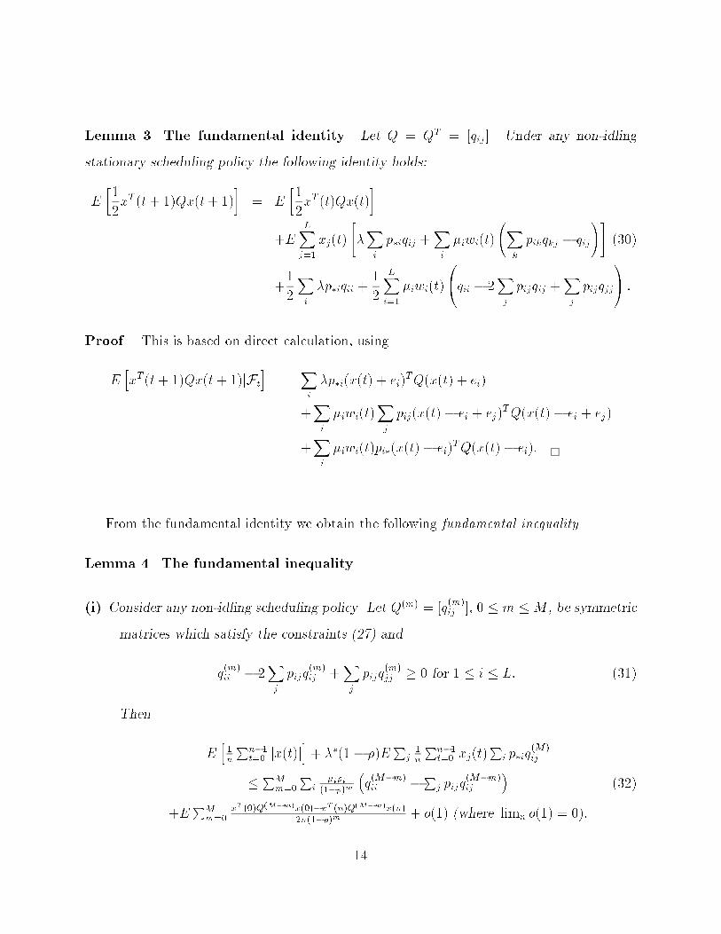
Lemma 3. The fundamental identity. Let Q = QT = [qij]. Under any non-idlingstationary scheduling policy the following identity holds:E�12xT (t+ 1)Qx(t+ 1)

�= E

�12xT (t)Qx(t)

�

+E LXj=1 xj(t)

"�Xi p�iqij +X

i �iwi(t) X

k pikqkj � qij!#

(30)

+12Xi �p�iqii + 1

2LXi=1 �iwi(t)

0@qii � 2Xj pijqij +X

j pijqjj1A :

Proof. This is based on direct calculation, usingE hxT (t+ 1)Qx(t+ 1)jFti = X

i �p�i(x(t) + ei)TQ(x(t) + ei)+Xi �iwi(t)Xj pij(x(t)� ei + ej)TQ(x(t)� ei + ej)+Xi �iwi(t)pi�(x(t)� ei)TQ(x(t)� ei):

From the fundamental identity we obtain the following fundamental inequality.Lemma 4. The fundamental inequality.

(i) Consider any non-idling scheduling policy. Let Q(m) = [q(m)ij ], 0 � m �M , be symmetricmatrices which satisfy the constraints (27) and

q(m)ii � 2Xj pijq(m)ij +Xj pijq(m)jj � 0 for 1 � i � L: (31)

ThenE h 1n Pn�1t=0 jx(t)j

i+ ��(1� �)EPj 1n Pn�1t=0 xj(t)Pi p�iq(M)ij� PMm=0Pi �i�i(1��)m

�q(M�m)ii �Pj pijq(M�m)ij � (32)+EPMm=0 xT (0)Q(M�m)x(0)�xT (n)Q(M�m)x(n)2n(1��)m + o(1) (where limn o(1) = 0):

14

(ii) Consider any non-idling scheduling policy with limn 1n Pn�1t=0 Ewi(t) = �i for all i. LetQ(m) = [q(m)ij ], 0 � m �M be symmetric matrices which satisfy (29). Then

E" 1n

n�1Xt=0 jx(t)j

#� ��(1� �)EXj

1n

n�1Xt=0 xj(t)

Xi p�iq(M)ij

� � MXm=0

Xi

�i�i(1� �)m

0@q(M�m)ii �Xj pijq(M�m)ij

1A (33)

�E MXm=0

xT (0)Q(M�m)x(0)� xT (n)Q(M�m)x(n)2n(1� �)m + o(1):

Proof. (i) With Q = Q(M), the term in (30) can be rewritten as�Xi p�iq(M)ij = ��Xi p�iq(M)ij � ��Xi p�iq(M�1)ij + (�� ��)Xi p�iq(M)ij + ��Xi p�iq(M�1)ij : (34)

Applying the fundamental identity with Q(M) in place of Q thus gives,E h12xT (t+ 1)Q(M)x(t+ 1)i = E h12xT (t)Q(M)x(t)i

+EPLj=1 xj(t)h��Pi p�i(q(M)ij � q(M�1)ij ) +Pi �iwi(t) �Pk pikq(M)kj � q(M)ij �i

+(�� ��)E hPLj=1 xj(t)PLi=1 p�iq(M)ij i+ ��E hPLj=1 xj(t)PLi=1 p�iq(M�1)ij i

+12 Pi �p�iq(M)ii + 12EPLi=1 �iwi(t) �q(M)ii � 2Pj pijq(M)ij +Pj pijq(M)jj � : (35)Now note that whenever xj(t) > 0 one of the quantities in fwi(t) : i 2 �(j)g is 1, while therest are zero, due to the assumption that the scheduling policy is non-idling. Hence,

xj(t) Xi2�(j)�iwi(t) X

k pikq(M)kj � q(M)ij!� xj(t)

"Maxi2�(j)�i

Xk pikq(M)kj � q(M)ij

!#:

Also, if � 6= �(j), then the wi(t)'s with i 2 � may be zero or one. Hence,

xj(t)Xi2� �iwi(t) X

k pikq(M)kj � q(M)ij!� xj(t)

24Maxi2� �i

Xk pikq(M)kj � q(M)ij

!+35 for � 6= �(j)

15

where a+ := Max(a; 0). Hencexj(t)Xi �iwi(t)

Xk pikq(M)kj � q(M)ij

!= xj(t)

24 Xi2�(j)�iwi(t)

Xk pikq(M)kj � q(M)ij

!

+ X� 6=�(j)

Xi2� �iwi(t)

Xk pikq(M)kj � q(M)ij

!35

� xj(t)"Maxi2�(j)�i

Xk pikq(M)kj � q(M)ij

!

+ X� 6=�(j)Maxi2� �i

Xk pikq(M)kj � q(M)ij

!+35 :Substituting this in (35) and using (27) yields,

E h12xT (t+ 1)Q(M)x(t+ 1)i � E h12xT (t)Q(M)x(t)i� Ejx(t)j+(�� ��)E hPLj=1 xj(t)PLi=1 p�iq(M)ij i+ ��E hPLj=1 xj(t)PLi=1 p�iq(M�1)ij i (36)

+E h12 Pi �p�iq(M)ii + 12EPLi=1 �iwi(t) �q(M)ii � 2Pj pijq(M)ij +Pj pijq(M)jj �i :Now note that since �i is the rate at which work arrives for bi,

1n

n�1Xt=0 Ewi(t) � �i + o(1); where limn!1 o(1) = 0:

Hence, using (31) and (8),1n Pn�1t=0

h12 Pi �p�iq(M)ii + 12 PLi=1 �iE(wi(t)) �q(M)ii � 2Pj pijq(M)ij +Pj pijq(M)jj �i

� PLi=1 �i�i�q(M)ii �Pj pijq(M)ij �+ o(1):

De�ne Xj(n) := 1n Pn�1t=0 xj(t). Summing (36), and taking expectations we obtainEjX(n)j � (�� ��)EPLj=1Xj(n)PLi=1 p�iq(M)ij � ��EPLj=1Xj(n)PLi=1 p�iq(M�1)ij� PLi=1 �i�i

�q(M)ii �Pj pijq(M)ij �+ 12 xT (0)Q(M)x(0)n � 12E xT (n)Q(M)x(n)n + o(1): (37)Similarly, for Q(m), 0 � m �M � 1, we obtain

�(�� ��)EPLj=1Xj(n)PLi=1 p�iq(m)ij � 1(m � 1)��EPLj=1Xj(n)PLi=1 p�iq(m�1)ij� PLi=1 �i�i

�q(m)ii �Pj pijq(m)ij �+ 12 xT (0)Q(m)x(0)n � 12E xT (n)Q(m)x(n)n + o(1): (38)16

Recursively substituting for EPLj=1Xj(n)PLi=1 p�iq(m)ij from (38) into (37) gives the result.(ii) The proof is similar.

5 Uniformly bounding functional expansionsIn this section we obtain the LPs for the uniformly bounding functional expansions.

To obtain uniformly upper bounding functional expansions for the mean number in thesystem as a function of �, we would like to neglect the term xT (n)Q(M�m)x(n) in (32).De�nition. A symmetric matrix Q is said to be copositive if xTQx � 0 for all x � 0.

We note that copositive matrices have been extensively studied (see Cottle, Habetler andLemke (1970), Murty and Kabadi (1987), and Andersson, Chang and Elfving (1993)), e.g., inlinear complementarity theory. They are characterized by the signs of certain determinants.However, testing for copositivity is NP-Complete. Clearly all positive semide�nite matrices(i.e., xTQx � 0 for all x), and all non-negative matrices (i.e., qij � 0 for all i; j), arecopositive.Theorem 3. Uniformly upper bounding functional expansions. Suppose Q(m), 0 �m �M , is a family of symmetric matrices satisfying (27,31) such that

MXm=0

1(1� �)mQ(M�m) is copositive, and (39)

Xi p�iq(M)ij � 0 for all j: (40)

Then, for every non-idling scheduling policy, for every arrival rate � in [0; ��), one haslim supn E

" 1n

n�1Xt=0 jx(t)j

#� �CM

(1� �)M + �CM�1(1� �)M�1 + � � �+ �C1

(1� �) + �C0; (41)

17

whereCm :=X

i �i��i0@q(M�m)ii �Xj pijq(M�m)ij

1A : (42)

If the scheduling policy is stationary, then the above bound also applies to the steady statevalue of Ejx(n)j.

Proof. Under (39), the term in the last summation in the RHS in (32), involving x(n), canbe dropped. Similarly, under (40), the second term on the LHS of (32) can be dropped.

This result provides a su�cient condition for stability for all arrival rates in the capacityregion 0 � � < ��. It also provides a bound on the order of the growth to in�nity in heavytra�c, i.e., pole multiplicity, as �% 1, Ejx(n)j = O � 1(1��)M

�.Any selection of the constants (C1; C2; . . . ; Cm) which satis�es the constraints of The-

orem 3 furnishes a functional upper bound on the mean number in the system. One canexploit the freedom that exists in the choice of the constants (C1; C2; . . . ; Cm) while meet-ing these constraints to choose a functional upper bound which has the lowest value at aparticular value �0 of the nominal load that may be of special interest.

For example, suppose one is interested in heavy tra�c performance, i.e., �0 = 1, or moreprecisely � % 1. Then one �rst minimizes the coe�cient CM = Pi �i��i

�q0ii �Pj pijq0ij�.

After minimizing CM , then one can still exploit the residual freedom by minimizing CM�1.Then one can minimize CM�2; CM�3; . . . ; C0 recursively as above.

On the other hand, if one is particularly interested in a nominal value of the load 0 <�0 < 1, then one minimizes

MXm=0

Cm(1� �0)m = MX

m=0Xi

�i��i(1� �0)m0@q(M�m)ii �Xj pijq(M�m)ij

1A :

18

After doing this there may still be residual freedom in choosing the coe�cients. This canbe exploited as one chooses. For example, one could minimize CM ; CM�1; . . . ; C0 as above ifthere is secondary interest in heavy tra�c behavior.

No matter how one exploits the freedom in choosing the coe�cients fCig which satisfythe constraints of Theorem 3, one always obtains a functional bound that is uniformly validfor all � in [0; 1) (provided of course that there is a feasible solution). Thus one can constructseveral such functional bounds and take their functional minimum which will yield anotherfunctional upper bound.

The constraints of Theorem 3 can be written as linear constraints on the variablesfqij; Cmg, except for the copositivity constraint (39). As noted earlier, the copositivity of amatrix is characterized by the signs of certain determinants, though testing for copositivityis NP-complete.

Instead of directly incorporating the copositivity constraints (39) in any optimizationprocedure for selecting the fCmg, one has two options. For the �rst option, one can simplyignore the copositivity constraint (39), and optimize the value of the Cm's as desired. Thenone can check whether the resulting optimal Q(m)'s are copositive. This yields a linearprogramming procedure followed by copositivity test. However it may be computationallycomplex for large problems due to the NP-Completeness of the copositivity test. The secondoption is to replace the copositivity condition (39) by the stronger non-negativity condition

Q(m) � 0; for 0 � m �M;where the matrix inequality is required to hold componentwise. Since these constraints arelinear, the entire procedure can then be performed by linear programming.

The algorithms above can be implemented beginning with M = 1, and increasing M byone at each step until one �nds the smallest value of M for which one has a feasible solutionto the constraints.

19

λ

Station 1 Station 2

µ1=3

µ3=3/2

µ2=3/2

µ4 =3

b1 b2

b4b3

Other search procedures for the smallest value of M can also be devised. One can easilynote that if there is a feasible solution for a particular value of M for M , then there is afeasible solution for all larger values of M � M . In particular, if fQ(0); Q(1); . . . ; Q(M)g isa feasible solution for M , then f0; 0; . . . ; 0; Q(0); Q(1); . . . ; Q(M)g is a feasible solution for M .Thus if one can �nd a large value of M for which there is a feasible solution, then one canproceed to �nd the smallest value of M for which there is a feasible solution by a bisectionsearch of f0; 1; 2; . . . ;Mg.

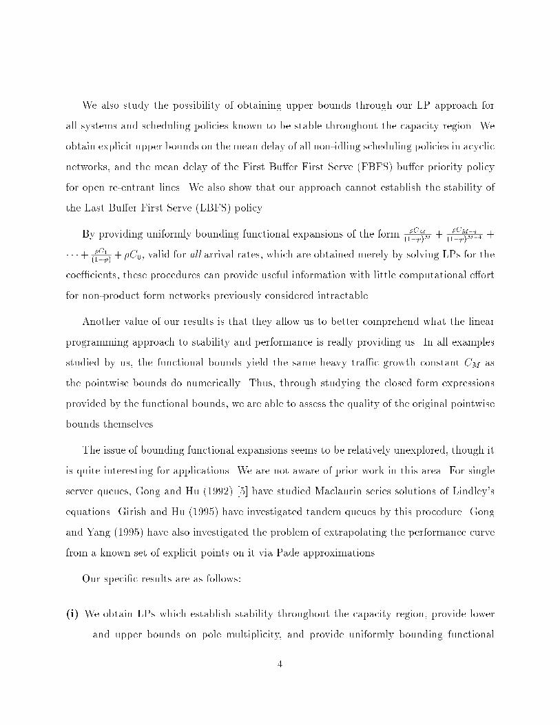
Example 1

Consider the system shown in Figure 2. The LP for the uniformly upper bounding functional

Figure 2: System of Examples 1, 2 and 3.

expansion is infeasible for M = 1. So we turn to M = 2. First we obtain the best constantsfor the heavy tra�c upper bound. We obtain a feasible solution, with a minimal value forC2 = 17=9. Recursively minimizing C1 (after �xing C2), and then C0 (after �xing C2 andC1), the uniformly upper bounding functional expansion obtained is,

Ejx(n)j � 17�9(1� �)2 +

11�9(1� �) for all � 2 [0; 1): (43)

20

The solution is

Q(0) =266664

1 2=3 2=3 02=3 2=3 2=9 2=92=3 2=9 2=3 �2=90 2=9 �2=9 2=9

377775 ; Q(1) =

2666641 1 1 11 11=9 5=9 11 5=9 5=9 1=31 1 1=3 1=3

377775 ; Q(2) = 0:

The matrix Q(0) is copositive but not non-negative. Like all the other upper bounds inthis paper, it is obtained by solving the LP without any copositivity constraint, and merelyverifying that the �nal answer is copositive. It may be noted that there is no non-negativefeasible solution for Q(0). In fact, at the nominal loading of 0.8 and larger, the originalStability LP of Kumar and Meyn (1995) does not possess a feasible non-negative solution,though it does possess a feasible copositive solution. This resolves in the negative (see Kumarand Meyn (1996)) an open problem concerning whether it is su�cient to restrict attentionto non-negative solutions for Q.

In Figure 3 we compare this bound (43) with the results of the pointwise bound LPs fromKumar and Kumar (1994). Computing lim�%1 (Upper Bound) (1� �)2 numerically gives avalue of 1.8889, which matches (43). The di�erence between the bounds, imperceptible inthe leftmost graph of Figure 3, is about 1:11� in light tra�c, and appears to be exactly 16�9(1��)in heavy tra�c.

Figure 3: Comparison of functional upper bound (43) with pointwise upper bounds inExample 1. The di�erence between them, imperceptible in the graph on the left, is moreperceptible in the other two graphs where the scales are linear in Log(jxj) and Log(1� �).

21

Next, as an illustration, we compute the functional bounds optimized for light tra�c,which corresponds to � in the neighborhood of �0 = 0. First we minimize C2 + C1 + C0.Then we �x C2 +C1 +C0 at its minimum value, and recursively minimize C2, then C1, and�nally C0, as above. This gives the bound

Ejx(n)j � 272�117(1� �)2 +

86�117(1� �) for all � 2 [0; 1); (44)

which comes from the solution,

Q(0) =26666416=13 32=39 32=39 032=39 32=39 32=117 32=11732=39 32=117 32=39 �32=1170 32=117 �32=117 32=117

377775 ; Q(1) =

266664

1 14=3 1 114=3 137=117 95=117 11 95=117 53=117 1=31 1 1=3 1=3

377775 ; Q(2) = 0:

Note that since both (43,44) are valid, one can take the minimum of them and obtain,Ejx(n)j � Minf 17�

9(1� �)2 +11�

9(1� �) ;272�

117(1� �)2 +86�

117(1� �)g for all � 2 [0; 1):

The following are the uniformly lower bounding functional expansion counterparts ofthese results. There is no need to require the copositivity condition (39), the positivitycondition (31), or to restrict attention to non-idling policies.Theorem 4. Uniformly lower bounding functional expansions. Suppose Q(m), 0 �m � M , is a family of symmetric matrices satisfying (29,40). Then for every schedulingpolicy, for every arrival rate � in [0; ��),lim infn E

" 1n

n�1Xt=0 jx(t)j

#� �CM

(1� �)M + �CM�1(1� �)M�1 + � � �+ �C1

(1� �) + �C0 for 0 � � < 1; (45)where

Cm :=Xi �i��i

0@X

j pijq(M�m)ij � q(M�m)ii1A (46)

If the scheduling policy is stationary, this lower bound also applies to the steady state valueof Ejx(n)j.

22

Proof. For a stationary scheduling policy with a �nite �rst moment it is shown in Kumarand Meyn (1996) that 1nE[xT (n + 1)Qx(n + 1) � xT (n)Qx(n)] ! 0 and so the second tolast term in (33) vanishes as n ! +1. (It is for this reason that unlike Theorem 3 nocopositivity condition is needed on Q). Also, for such a policy 1n Pn�1t=0 E(wi(t)) ! �i. (Itis for this reason that unlike Theorem 3 there is no need for the positivity condition (31)).Hence the bound (45) follows from Lemma 4.ii for stationary non-idling scheduling policieswith a �nite �rst moment. If a stationary policy does not have a �nite �rst moment, then thelower bound (45) holds trivially. Thus the bound holds for all stationary non-idling policies.

From Borkar (1983) it follows that given an initial condition for the Markovian net-work there exists a stationary non-idling scheduling policy that is optimal in the class ofall non-anticipative non-idling scheduling policies, for the problem of minimizing the longterm average of the mean number in the system. Hence the lower bound (45) applies to allnon-idling policies. Finally, given any policy � that is not non-idling, one can construct anew non-idling policy e� under which every station works on a customer at a time that �would have worked on it, provided that under e� that same customer is present at the stationat that time, but e� is non-idling since it works on an available customer in First Come FirstServe order at other times. Under such a policy e� every customer leaves the system no laterthan it would have under �. Thus, for every policy, there is a non-idling policy that is atleast as good. Hence the lower bound (45) applies to all policies.

We thus obtain a lower bound (using Knuth's notation) on the growth rate in heavytra�c, Ejx(n)j = � 1(1��)M

�, and a bound on pole multiplicity. The best constants Cm fora particular nominal load �0 are found as in the case of the upper bounds. Since there is nocopositivity condition to check, these are purely linear programming procedures.

23

Example 2

Consider the system shown in Figure 1. First we obtain the best coe�cients for the heavytra�c region. The LP for the uniformly lower bounding functional expansion in (i) aboveyields Q(0) � 0 when M = 2. So we turn to M = 1. This gives

Ejx(n)j � 7�9(1� �) +

7�9 for all � 2 [0; 1): (47)

The solution is

Q(0) =266664

�1 �2=3 �2=3 0�2=3 �4=9 �4=9 0�2=3 �4=9 �4=9 00 0 0 0

377775 and Q(1) =

2666640 0 0 00 �1=9 1=9 00 1=9 1=9 1=30 0 1=3 �1=3

377775 :

The pointwise lower bounds in Kumar and Kumar (1994) numerically give lim�%1(1� �)(Lower Bound) = 0:7778. Thus the uniformly lower bounding functional expansion (47)directly obtains the same constant. The graphs in Figure 4 compare the uniformly lowerbounding functional expansion (47) with the pointwise bounds. The di�erence between thetwo bounds is about 0:44� is light tra�c, and about 1:78� in heavy tra�c.

Figure 4: Comparison of functional lower bound (47) with pointwise lower bounds forsystem of Example 2.

24

Next we �t a bound optimized for the low tra�c region �0 = 0. First we maximizeC2 + C1 + C0. Then �xing C2 + C1 + C0 at its maximum value, we recursively maximizeC2; C1, and C0. This yields

Ejx(n)j � 16�9 for all � 2 [0; 1); (48)

which comes from the solution,

Q(0) =266664

0 1=3 0 01=3 �4=9 0 00 0 �2=3 00 0 0 �1=3

377775 and Q(1) = 0:

Since both bounds are uniformly valid, we can take their functional maximum, and obtainEjx(n)j � Maxf 7�

9(1� �) +7�9 ;

16�9 g for all � 2 [0; 1):

Consider now a bu�er priority policy �. We have seen earlier that the additional constraint(11) is satis�ed in the primal. The dual LP correspondingly restricts the \Maxi2�(j)" in (27)and (29) to \Maxfi:i2�(j) and �(i)��(j)g. The uniformly lower and upper bounding functionalexpansions carry over with this change.Theorem 5. Uniformly bounding functional expansions for bu�er priority poli-cies. Consider a bu�er priority policy �. The bounds of Theorems 3 and 4 hold with themodi�cation that \Maxi2�(j)" in (27) and (29) is replaced by \Maxfi:i2�(j) and �(i)��(j)g."

Example 3

Consider the system shown in Figure 1. There are four bu�er priority policies �LBFS =(4; 3; 2; 1), �FBFS = (1; 2; 3; 4), �3214 and �1432. The uniformly lower and upper bounding

25

Functional Lower Bound Functional Upper Bound�LBFS 11�9(1��) + 7�9 17�6(1��) + 2�3�FBFS Maxf 7�3(1��) � 7�; 16�9 g 11�2(1��)�3214 7�9(1��) + 7�9 17�9(1��)2 + 11�9(1��)�1432 29�24(1��) + 25�48 17�6(1��) + 2�3

Figure 5: Uniformly lower and upper bounding functional expansions for all bu�er prioritypolicies in system of Example 3.

functional expansions, both optimized for the heavy tra�c region, are shown in Figure 5.For �FBFS we take the maximum of the heavy and light tra�c optimized bounds. In allcases, the coe�cient CM of the highest power is the same as that obtained numerically inthe limit from the pointwise bounds. It is worth noting that for �LBFS the functional lowerbound appears to coincide exactly with the pointwise lower bounds for all values of �.

In all the Examples 1, 2 and 3, the heavy tra�c growth constant CM produced by thefunctional bound LPs has coincided with the value computed numerically from the pointwisebound LPs. Hence the closed form solution provided by the functional bound LPs allows usto comprehend the quality of the results provided by the original pointwise bound LPs.

6 Reduced dimensional LP for the functional lowerbound for balanced systems

We now explicitly describe a family of feasible solutions of the LP for the uniformly lowerbounding functional expansions for balanced systems where �� � � for all �. These explicitsolutions provide functional lower bounds of the form Ejx(n)j � C1�1�� . They are describedby parameters that can be optimized through considerably lower dimensional LPs. Whilethe original LP for M = 1 features L(L+ 1) variables �L(L+1)2 variables for each of Q(0) and

26

Q(1)�, our explicit solution only features S(S+1)2 variables, where S is the number of stations,which is in many applications of interest far smaller than the number L of bu�ers.

The feasible solutions are expressed in terms ofW�i, the mean work remaining to be doneon a customer in bu�er bi by station �, prior to that customer's exit from the system. Theyare obtained as the unique solution of the equations,

W�i = 1�i1(i 2 �) +X

j pijW�j for all i: (49)

The key idea is to restrict attention to quadratics in the mean remaining work w� :=PiW�ixi for stations, rather than more general quadratics in the system state consistingthe number customers in each bu�er. Speci�cally, instead of considering quadratics such asPij qijxixj, one restricts attention to quadratics such as �P�� a��0w�w�0 . Thus we look forfeasible solutions of the form Q(m) = �W TA(m)W where W := [W�i]. In what follows wedetail a construction for Q(0) which with M = 1 and Q(1) = 0 yields a feasible solution. Ourconstruction works only for balanced systems with �� � �, i.e., those systems for which allstations are equally loaded. The result is a lower bound with a pole multiplicity of order 1.In our numerical studies we have been unable to �nd any queueing network for which a lowerbound with pole multiplicity greater than or equal to 2 can be established.

The following lemma provides the details of our construction.Lemma 5. Consider a balanced system, i.e., �� � � for all �. Let A = AT = [a��0 ] be anS � S matrix which satis�es,

X��0 a�0�W�j � 1 for all j; (50)

X� a�0�W�j � 0 for all �0 and j; (51)

a��0 = a�0� for all �; �0: (52)

27

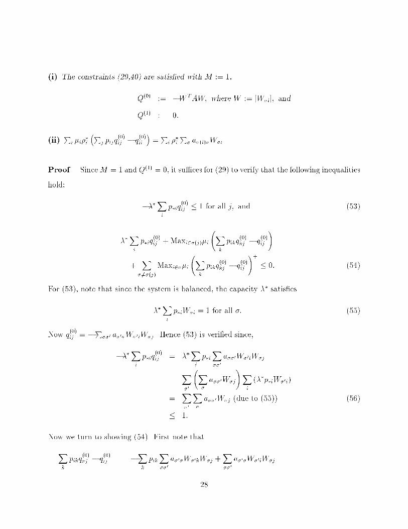
(i) The constraints (29,40) are satis�ed with M := 1,Q(0) := �W TAW; where W := [W�i]; andQ(1) := 0:

(ii) Pi �i��i�Pj pijq(0)ij � q(0)ii � = Pi ��i P� a�(i)�W�i.

Proof. SinceM = 1 and Q(1) = 0, it su�ces for (29) to verify that the following inequalitieshold:

���Xi p�iq(0)ij � 1 for all j; and (53)

��Xi p�iq(0)ij +Maxi2�(j)�i X

k pikq(0)kj � q(0)ij!

+ X� 6=�(j)Maxi2��i

Xk pikq(0)kj � q(0)ij

!+� 0: (54)

For (53), note that since the system is balanced, the capacity �� satis�es��Xi p�iW�i = 1 for all �: (55)

Now q(0)ij = �P��0 a�0�W�0iW�j. Hence (53) is veri�ed since,���Xi p�iq(0)ij = ��Xi p�iX��0 a��0W�0iW�j

= X�0 X

� a��0W�j!X

i (��p�iW�0i)= X

�0X� a��0W�j (due to (55)) (56)

� 1:Now we turn to showing (54). First note thatXk pikq(0)kj � q(0)ij = �Xk pikX��0 a�0�W�0kW�j +X

��0 a�0�W�0iW�j

28

= �X��0"W�0i � 1

�i1(i 2 �0)#a�0�W�j +X

��0 a�0�W�0iW�j (from (49))= 1

�iX� a�(i)�W�j (57)

� 0 (from (51));which also establishes (ii) as a by product of (57).

HenceLHS of (54) = ��Xi p�iq(0)ij +X

��0 a��0W�j= 0 (from (56);

which proves (54), and thus (i), since (40) trivially holds.The equality in (ii) follows from (49).

Once we have discovered constraints on A(0) which guarantee that the resultingfQ(0); Q(1) = 0g are feasible, we can optimize the lower bound by linear programming.Thus we obtain the following reduced dimensional LP for the functional lower bound.Theorem 6. Reduced dimensional LP for functional lower bound for balancedsystems. Consider a balanced system. Let C1 be the value of the LP,

MaxXi ��i X� a�(i)�W�isubject to (50, 51, 52). Then, for any scheduling policy,

lim infN1N

N�1Xn=0 Ejx(n)j �

�C11� �: (58)

29

λ

Station

µ1

µ2

µl

b1

b2

bl

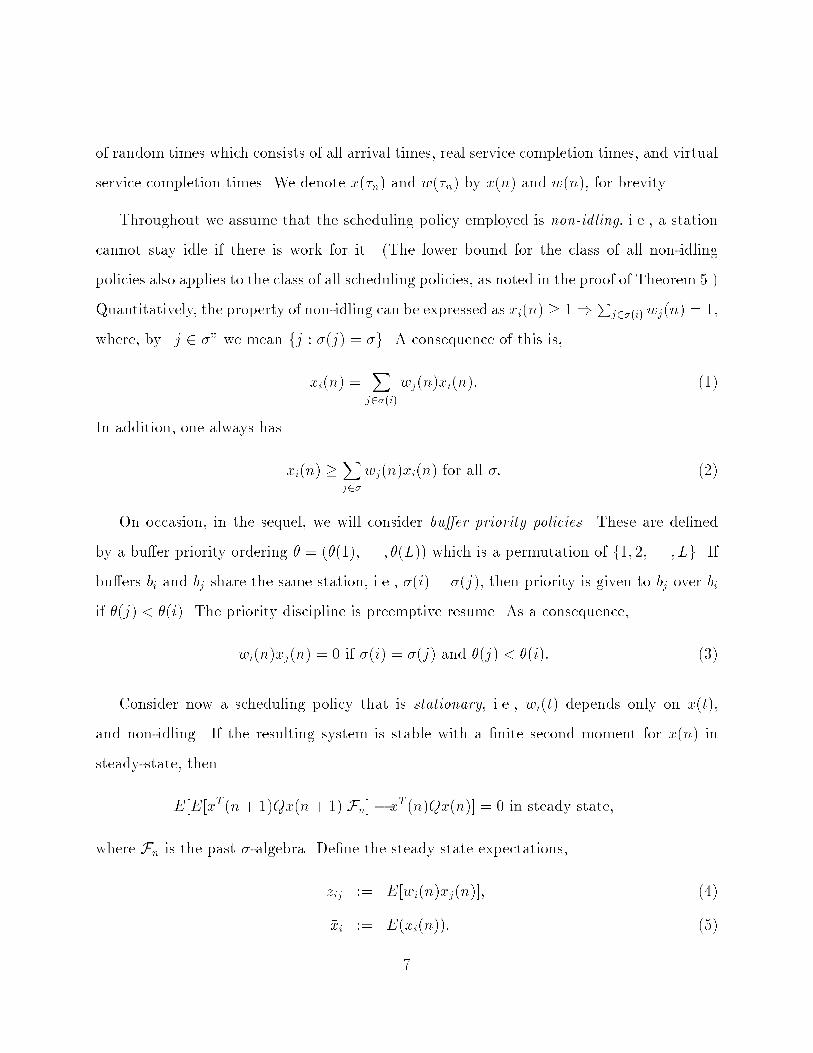
7 Asymptotic heavy tra�c domination of thePollaczek-Khintchine bound

We now show that the functional lower bound (58) produced by the reduced dimensionalLP of Theorem 6 is always at least as good asymptotically in heavy tra�c as a bound fornetworks obtainable from the Pollaczek-Khintchine formula which captures the behavior ofany one bottleneck. More precisely, we show that as �% 1 the limiting ratio of (58) to thelower bound obtained from the Pollaczek-Khintchine formula is guaranteed to be at leastone. We also provide an example where the limiting ratio is strictly larger than one. Thisexample shows that our functional lower bound (58) (and thus also (45)) captures nontrivialinteractions between multiple bottleneck stations in heavy tra�c.

Recall that the Pollaczek-Khintchine formula for the mean number of customer-s in an M=G=1 queue operated under the First Come First Serve (FCFS) policy is2���2+�2var(service time)2(1��) . We can apply this formula to calculate a lower bound on the meannumber in the system shown in Figure 6 consisting of a single station revisited several times.

Figure 6: A single station with multiple revisits.30

Under any non-idling scheduling policy the work in this system is conserved. It is also easy tosee that the mean number of customers in the system is a minimum when the Last Bu�er FirstServe bu�er priority policy is used, which gives priority to the bu�ers fb`; b`�1; . . . ; b1g in thatorder. The resulting queueing system is equivalent, in terms of the number of customers in thesystem at any given time, to anM=G=1 queue where each customer's service time is the sumof ` independent exponentially distributed random variables with means 1�1 ; 1�2 ; . . . ; 1�` , whenit is operated under the FCFS policy. Such a combined service time has mean Pi=1 1�i andvariance Pi=1 1�2i , with � = �Pi=1 1�i . Thus, we obtain that the mean number of customersunder any non-idling policy (and in fact under any scheduling policy) for the single stationmultiple revisit system of Figure 6 is lower bounded by 2���2+�2Pi=1 1�2i2(1��) .

Using this, we can derive a lower bound for any open re-entrant line, i.e., a network asin Section 2 with every pij either 0 or 1 (as in Figure 2). Let � be a �xed station in sucha network. Now if all customers spend zero time at all bu�ers in the network, except thebu�ers of station �, then one obtains a network of the form shown in Figure 6, which hasthe lower bound 2���2+�2Pi2� 1�2i2(1��) . It is easy to show that this lower bound is also a lowerbound on the number of customers in the original network where the service times at allother stations are not zero.

For every station �, one therefore obtains such a lower bound, from which it follows bymaximizing over � that for the open re-entrant line, under any scheduling policy in steady-state,

E j x(t) j � Max�2�� �2 + �2Pi2� 1�2i2(1� �) : (59)

We call this the Pollaczek-Khintchine lower bound. In a sentence, it captures the worstbottleneck in the system, when all stations except one, are made transparent to customers.

We will show below in Theorem 7 that if we consider the functional lower bound of theprevious section with the further restriction that A is a non-negative matrix, then the value

31

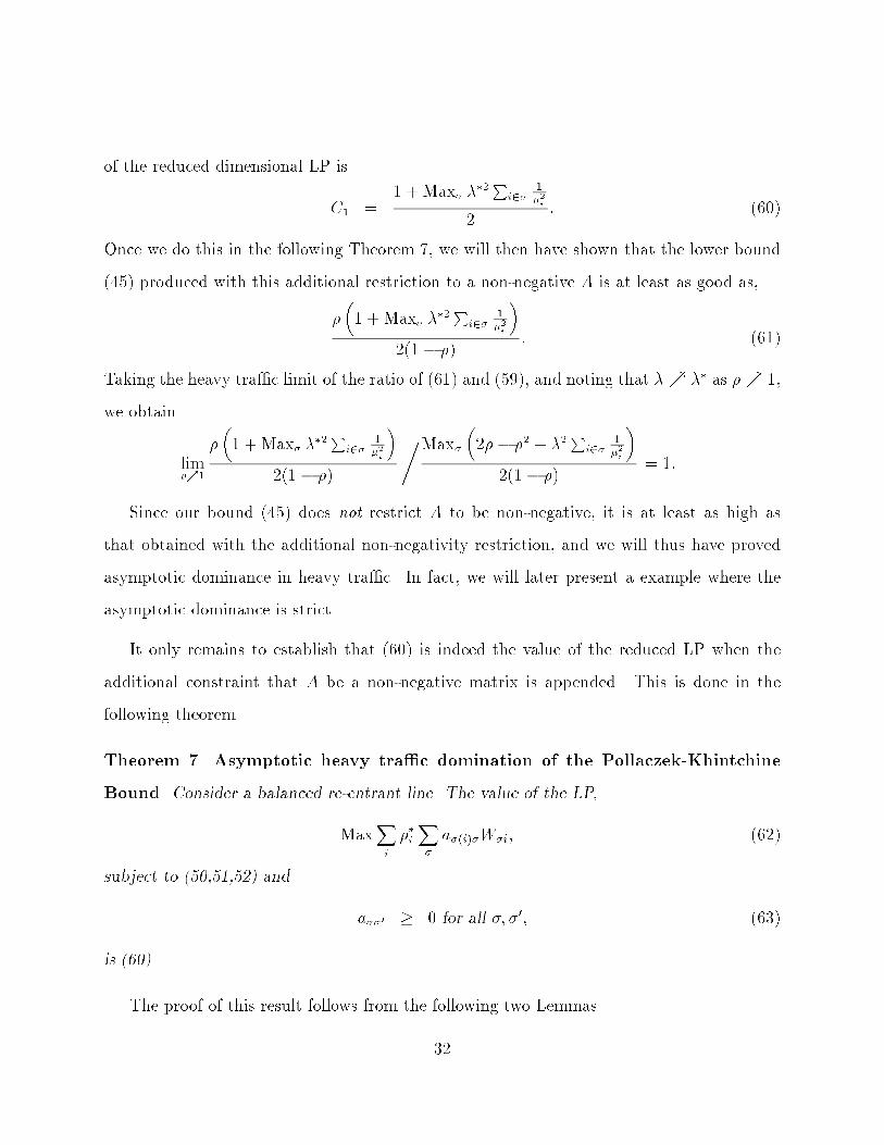
of the reduced dimensional LP isC1 = 1 +Max� ��2Pi2� 1�2i2 : (60)

Once we do this in the following Theorem 7, we will then have shown that the lower bound(45) produced with this additional restriction to a non-negative A is at least as good as,

��1 +Max� ��2Pi2� 1�2i

�

2(1� �) : (61)Taking the heavy tra�c limit of the ratio of (61) and (59), and noting that �% �� as �% 1,we obtain

lim�%1��1 +Max� ��2Pi2� 1�2i

�

2(1� �),Max�

�2�� �2 + �2Pi2� 1�2i

�

2(1� �) = 1:Since our bound (45) does not restrict A to be non-negative, it is at least as high as

that obtained with the additional non-negativity restriction, and we will thus have provedasymptotic dominance in heavy tra�c. In fact, we will later present a example where theasymptotic dominance is strict.

It only remains to establish that (60) is indeed the value of the reduced LP when theadditional constraint that A be a non-negative matrix is appended. This is done in thefollowing theorem.Theorem 7. Asymptotic heavy tra�c domination of the Pollaczek-KhintchineBound. Consider a balanced re-entrant line. The value of the LP,

MaxXi ��i X� a�(i)�W�i; (62)subject to (50,51,52) and

a��0 � 0 for all �; �0; (63)is (60).

The proof of this result follows from the following two Lemmas.32

Lemma 6. The value of the LP in Theorem 7 is��2Max�;�0 hPi2�0 1�iW�i +Pi2� 1�iW�0ii

2 :

Proof: De�ne c�0� := Pi2�0 ��iW�i. Using the symmetry of a��0 we can write the objective(62) as,

Xi ��i X� a�(i)�W�i = X

��0 a�0�Xi2�0 �

�iW�i= X

��0 a�0�c�0�= X

��0 a�0�(c��0 + c�0�)

2 : (64)

Now note that since the system is a re-entrant line and is also balanced, from (55) wehave W�1 = 1�� for all �. Hence the constraint (51) for j = 1 is,

X��0 a�0� � ��:

Fix a choice of � and �0 such that c� �0 + c�0� � c��0 + c�0� for all �, �0. Since a�0� � 0,it follows that an optimal \allocation" of the a�0�'s in the LP is to set a� �0 = a�0� = ��2if � 6= �0, or a� � = �� if � = �0, and set all other a��0 's to zero. Since this is a feasibleallocation, the result follows from (64) upon noting that ��i = ���i .

Lemma 7.Xi2�0

1�iW�i +X

i2�1�iW�0i = 1

��2 + 1(� = �0)Xi2�1�2i : (65)

Proof. Let ai := 1(i 2 �) and bi := 1(i 2 �0). ThenXi2�0

1�iW�i +X

i2�1�iW�0i = X

i1�i bi

Xj�i

1�j aj +

Xi

1�iai

Xj�i

1�j bj

33

b1 b2

b4

b5

b3

b6Station 1

Station 2

Station 3

µ1=3

µ3=3/2

µ2=10/9

µ5=10

µ4=6

µ6=6/5

λ

= XiXj�i

1�i�j biaj +

XiXj�i

1�i�j aibj

= XiXj

1�i�j biaj +

Xi

1�2i aibi

= X

i1�i bi

!0@X

j1�j aj

1A+X

i2�1�2i 1(i 2 �)1(i 2 �0)

= 1��2 + 1(� = �0)Xi2�

1�2i :

Now we provide an example to show that when the sign of a��0 is unrestricted as in(45), it can give a strictly better lower bound than (60). Hence the asymptotic dominancein heavy tra�c of our lower bound (45) over the Pollaczek-Khintchine bound (59) is strict.Thus we see that the lower bound can capture complicated interactions between multiplebottleneck stations.

Example 4

Consider the system of Figure 7.

Figure 7: System of Example 4.

34

The optimal non-negative A gives C1 = 91=100, with

ANon-negative =2640 0 00 1 00 0 0

375 :

It clearly captures only the behavior of the single bottleneck Station 2.On the other hand, the optimal sign inde�nite solution for A is,

ASign inde�nite =264

99=467 �75=467 9=467�75=467 500=467 09=467 0 0

375 :

It clearly captures the interactions between all the three bottleneck stations, and it gives thestrictly larger value of the constant C1 = 466=467.

8 Explicit pointwise upper boundsThe only topological con�gurations which have been proved to be stable for all non-idlingpolicies throughout the capacity region [0; ��) are acyclic networks. The only bu�er prioritypolicies which have been proved stable throughout the capacity region [0; ��) for all re-entrant lines are the First Bu�er First Serve Policy (FBFS) �FBFS = f1; 2; . . . ; Lg, and theLast Bu�er First Serve Policy (LBFS) �LBFS = fL;L�1; . . . ; Lg, see Lu and Kumar (1991),Dai (1995), Kumar and Kumar (1995), and Dai and Weiss (1994). It is only for such systemswhich are provably stable throughout [0; ��) that one can hope to establish functional upperbounds.

In the following Sections 9 and 10, we are able to provide upper bounds for all acyclictopologies for all non-idling policies, and the FBFS policy for all re-entrant lines, but �rstwe demonstrate by a counterexample that the method of using quadratic functions cannotgive the proof of stability for LBFS throughout the capacity region.

35

b4 b4

λ

Station 1 Station 2

µ1=10 µ2=10/3

µ3=5

b1 b2

µ4 =10/8

Example 5: Unbounded pointwise upper bound LP for LBFS

Consider the system shown in Figure 8, operating under the LBFS policy.

Figure 8: System of Example 5 for which pointwise upper bound LP for the LBFS policy isunbounded.

The pointwise upper bound LP is,Min�

LXi=1 qii �

L�1Xi=1 qi;i+1

!

subject to:�q1j +Maxfi:i2�(j) and i�jg�i(qi+1;j � qij) + Maxi 62�(j)�i(qi+1;j � qij)+ � �1:

It is the dual of the pointwise upper bound LP in Theorem 2. If the mean number inthe system is �nite in steady state, then the value of this LP is an upper bound on it. Asshown in Figure 9, the value is unbounded for 0:8892 < � < 109 = ��. As a consequence, theLP for the uniformly upper bounding functional expansion is infeasible.

36

Figure 9: Plot of value of pointwise upper bound LP for LBFS policy in Example 5. It isunbounded for � > 0:8892.

9 Explicit upper bound for the FBFS policyIn this section we determine an upper bound on the pole multiplicity for re-entrant linesoperating under the FBFS policy. We will do so by directly determining an explicit feasiblesolution for the original pointwise upper bound LP itself. Our method will provide a func-tional form for the Q matrix for the pointwise upper bound LP, and we establish the polemultiplicity upper bound by studying this. With this result, the FBFS policy becomes theonly one known, to the best of our knowledge, for which a pole multiplicity upper bound isavailable for all re-entrant lines.

If the mean number in the system is �nite, a pointwise upper bound on the FBFS policy,for each arrival rate �, is given by the value of the pointwise upper bound LP of Theorem2. Its dual is,

Min � LXi=1 qii �

L�1Xi=1 qi;i+1

!

subject to,�q1j +Maxfi:i2�(j) and i�jg�i(qi+1;j � qij) + X

� 6=�(j)Maxi2��i(qi+1;j � qij)+ � �1: (66)

37

Let us append the following non-negativity condition and call it the Stability LP,qij = qji � 0: (67)

Then, it follows that if there is a feasible solution, it is automatically copositive, and so themean number in the system is indeed �nite, and hence the value of the Stability LP is apointwise upper bound, see Kumar and Meyn (1996).Theorem 8. Upper bound for FBFS. Consider a re-entrant line operating under theFBFS policy.(i) Let

b� := Maxi2�W�;i (= W�;1) : (68)For a �xed �1 > 0, recursively de�ne,

�i+1 = �i Min(Min1�j�i�1 W�(i)j

W�(i+1)j ;�iW�(i)i � �b�(i)2�iW�(i+1);i

)for 1 � i � L� 1:

(For i = 1, �2 is taken equal to the second term). Now scale �1, thus rescaling all theother �js, so that

�j Max8<:�b�(j) � 1;

��b�(j) � �jW�(j)j�2

9=; � �1 for all j: (69)

Then using the notation i _ j := max(i; j) and i ^ j := min(i; j),qij := �i_jW�(i_j);i^j

satis�es the constraints (66,67) of the Stability LP.(ii) Hence E(xn) � �(PLi=1 qii �PL�1i=1 qi;i+1) in steady state.

Proof. Note �rst that since �1 > 0, it follows that �i > 0 for all i, since �iW�(i)i � �b�(i) �1� �b�(i) > 0. Moreover each �i < +1 since W�(i+1)1 > 0 for 1 � i � L� 1.

We will now bound �i(qi+1;j � qij) by considering several cases.38

Case i: i < j�i(qi+1;j � qij) = �i(�jW�(j);i+1 � �jW�(j)i) = �1(i 2 �(j))�j � 0:

Case ii: i > j�i(qi+1;j � qij) = �i(�i+1W�(i+1)j � �iW�(i)j) � 0:

Case iii: i = j�j(qj+1;j � qjj) = �j(�j+1W�(j+1)j � �jW�(j)j)

� �j �j �jW�(j)j � �b�(j)

2�jW�(j+1)j W�(j+1)j � �jW�(j)j!

= ��j �jW�(j) + �b�(j)2

< 0:

HenceLHS of (66) = ��jW�(j)1 +Maxfi:i2�(j) and i�jg

8<:��j;

��j ��jW�(j)j + �b�(j)�2

9=;

= �j Max((�b�(j) � 1); (�b�(j) � �jW�(j)j)

2)

(70)< 0:

After scaling as in (69), �1 is chosen to makeLHS of (66) � �1 for 1 � j � L;

thus satisfying (66).

As a corollary, from Kumar and Meyn (1995) it follows that FBFS is stable in thefollowing very strong sense.

39

Corollary. Exponential stability of FBFS. Under FBFS, for any 0 � � < ��, the systemis e�x-uniformly ergodic for some small � > 0. In particular it has moments of all polynomialorders and even an exponential moment, and they all converge geometrically fast to theirsteady state values.

Next we obtain the upper bound on the pole multiplicity of the growth rate of FBFS.We study the behavior when � is close to �� by employing a slightly di�erent constructionwhich separates the bottleneck stations and their last bu�ers, from the others.Theorem 9. Upper bound on pole multiplicity of FBFS. Under the FBFS policy,

Ejxnj = O 1(1� �)B

!; (71)

where B is the number of bottleneck stations.

Proof. The proof is again by constructing an explicit solution for Q. We separate thelast bu�ers at the bottleneck stations from the others. With B := f� : ��W�1 = 1g = set ofbottleneck stations, let

L := fi : i = maxfj : j 2 �g for some � 2 Bg= set of last bu�ers at the bottleneck stations,

let�i := Min1�j�i�1 W�(i)j

W�(i+1)j for 2 � i � L� 1;��i := �iW�(i)i � ��b�(i)

2�iW�(i+1)i for i 62 L; 1 � i � L� 1; (72)�i(�) := �iW�(i)i � �b�(i)

2�iW�(i+1)i = 1� ��(i)2�iW�(i+1)i for i 2 L; 1 � i � L� 1:

Let i(�) :=

( �i := Minf�i; ��i g for i 62 L; 1 � i � L� 1;Minf�i; �i(�)g for i 2 L1; 1 � i � L� 1:

40

With �1 := 1, we recursively set�i+1 := �i i(�) for i = 1; 2; . . . ; L� 1:

We note that since �iW�(i)i = 1 = ��b�(i) for i 2 L, �i(��) = 0, and so i(�) = �i(�) for all i 2 L; for � in some open interval (�� � �; ��): (73)

Consequently,�i+1 = Y

1�k�ik 62L �k Y

1�k�ik2L k(�) for 1 � i � L� 1; and � in (�� � �; ��): (74)

De�ne qij := �i_jW�(i_j)i^j.We will henceforth restrict attention to � in (�� � �; ��). Exactly as in Theorem 8, we

can verify that the bounds of Cases i, ii, and iii hold, and that (70) holds.Now we note that with �1 := 1, the objective function satis�es

� LXi=1 qii �

L�1Xi=1 qi;i+1

!= �

LXi=1 �iW�(i)i �

L�1Xi=1 �i+1W�(i+1)i

!

� � LXi=1 �iW�(i)i (75)

� c; where c does not depend on �:Now we investigate (70) since we want to scale �1, which will result in the scaling of (75), sothat the LHS of (66) is bounded above by (�1).

For j 2 � 62 B, ��(j)��jW�(j)j = �W�(j)1��jW�(j)j � ��W�(j)1� 1 � c0 < 0 for some c0.Hence for j 2 � 62 B, LHS of (66) � �12�jc0. For j 2 � 2 B, ��(j)��jW�(j)j � ��(j)�1 = ��1.Hence for j 2 � 2 B, LHS of (66) � � �j2 (1 � �). Therefore, dividing �1 by c00(1 � �)Minj�jyields (66). Noting from (72, 73, 74) that �i+1 � c000(1� �)B�1, the bound (71) follows.

41

10 Upper bound for acyclic systemsIn this section we obtain an explicit upper bound for all acyclic networks, i.e., systems forwhich

�(i+ 1) 6= �(i) implies that �(j) 6= �(i) for all j � i+ 1:Note that immediate revisits to stations are allowed. This is again done through an explicitfeasible solution for the original pointwise upper bound LP itself.

De�ne b� as in (68), anda� := MiniW�i (= 1

�i� where i� := ArgMax fi : i 2 �g):

Theorem 10. Upper bound for acyclic systems. Let

�1 := Max�264 1a�Q�s=1 (1��bs)2 Q��1s=1 a2sb2s+1

375

��+1 := ��(1� �b�2 ) a2�b2�+1 for � = 1; 2; . . . ; S � 1:

Thenqij := ��(i)_�(j)W�(i)_�(j);iW�(i)_�(j);j

satis�es�q1j +Maxfi:i2�(j)g�i(qi+1;j � qij) + X

� 6=�(j)Maxi2��i(qi+1;j � qij)+ � �1: (76)

Hence, for all non-idling policies,E(xn) � �

LXi=1 ��(i)W

2�(i);i �L�1Xi=1 ��(i+1)W�(i+1);iW�(i+1);i+1

!for all 0 � � < ��

= O( 1(1� �)B ):

42

Proof: Note that�� = �1

��1Ys=1

(1� �bs)2

a2sb2s+1 �2

a�(1� �b�) for � � 2:We bound �i(qi+1;j � qij).

Case i: �(i) < �(j)�i(qi+1;j � qij) = �i(��(j)W�(j);jW�(j);i+1 � ��(j)W�(j);jW�(j);i)

= 0:

Case ii: �(i) � �(j) and �(i+ 1) = �(i)�i(qi+1;j � qij) = �i(��(i)W�(i);jW�(i);i+1 � ��(i)W�(i);jW�(i);i)

= ���(i)W�(i);j� 0:

Case iii: �(i) � �(j) and �(i+ 1) = �(i) + 1�i(qi+1;j � qij) = �i ���(i)+1W�(i)+1;jW�(i)+1;i+1 � ��(i)W�(i);jW�(i);i�

= 1a�(i)

0@��(i) (1� �b�(i))

2a2�(i)b2�(i)+1 b

2�(i)+1 � ��(i)W�(i);ja�(i)1A

= ��(i) (1� �b�(i))

2 a�(i) �W�(i);j!

� 0 (since a�(i) � W�(i);j):

Hence,LHS of (76) � ���(j)b�(j)W�(j);j +Max

((���(j)W�(j);j); ��(j)1� �b�(j)

2 a�(j) � ��(j)W�(j);j)

= ���(j)b�(j)W�(j);j + ��(j) (1� �b�(j))2 a�(j) � ��(j)W�(j);j

43

λ

µ1 µ2

b1 b2

= (�b�(j) � 1)��(j)W�(j);j + (1� �b�(j))2 ��(j)a�(j)

� �b�(j) � 12 ��(j)a�(j) (since a�(j) � W�(j);j)

� �1:

If the pole multiplicity bound is too loose, one may wonder whether that is due to thefunctional bound LPs or the original pointwise bounds themselves. The following tandem ex-ample shows that the pointwise bounds themselves are simply not cognizant of distributionalresults such as Burke's' Theorem.

Example 6: Upper bound for tandem systemConsider the tandem system shown in Figure 10.

Figure 10: Tandem system of Example 6.In the balanced case �1 = �2 = ��, the functional upper bound LP gives,

M = 2; C2 = 1; C1 = 1; C0 = 0; Q0 = 1��" 1 00 0

#; Q(1) = 1

��" 1 11 1

#; Q(2) = 0;

which yields the functional upper bound,Ejx(n)j � �

(1� �)2 +�

1� �:The loose pole multiplicity bound of 2 originates in the original pointwise bounds themselves,since the pointwise LP gives

lim�%1(1� �)2 Upper Bound = 1:44

However in the unbalanced case, one does obtain �rst order bounds. If �1 > �2 = ��,then

M = 1; Q(0) = 1��" �1�1��� 1

1 1#; Q(1) = 0;

is feasible. This gives the upper bound,Ejxnj � ( �1�1��� )�1� � :

If �2 > �1 = ��, thenM = 1; Q(0) = 1

��" 1 00 0

#; Q(1) =

" 0 00 1�2���

#;

is feasible. This givesEjxnj � �

1� � + ����2 � �� :

11 Concluding remarksFor the performance analysis of open Markovian queueing networks, we have obtained LPsthat provide uniformly bounding functional expansions for the performance throughout thecapacity region. We have shown that our bounds can capture nontrivial interactions betweenmultiple bottleneck stations in heavy tra�c.

Several interesting open questions remain. Little appears to be known concerning thepole multiplicity in heavy tra�c. This is not surprising since until recently even the issueof stability was not regarded as a major issue. However, it is important to characterizepole multiplicity as well as the growth constants if one wants to comprehend the behaviorof a network as tra�c increases. A pole multiplicity of M corresponds to a steady statedistribution �(jxj = n) = (n(M�1)�n). Currently we are not aware of any examples of high

45

pole multiplicity, though instability for arrival rates short of capacity corresponds to a polemultiplicity of M = +1. This is a challenging area for the future, as is the whole issue ofobtaining uniform functional bounds. By considering a scheduling policy which applies astable stationary policy o� of a large compact set in the state-space, but which within thecompact set applies a destabilizing policy, it should be possible to obtain pole multiplicitieswhich are arbitrarily high. Whether such large pole multiplicities can result from bu�erpriority policies is a more challenging problem. We conjecture that this may be possible too.Acknowledgments The authors thank all those involved in the reviewing process for theire�orts.

References[1] P. R. Kumar and S. P. Meyn, \Stability of queueing networks and scheduling policies,"

IEEE Transactions on Automatic Control, vol. 40, pp. 251{260, February 1995.[2] S. Kumar and P. R. Kumar, \Performance bounds for queueing networks and scheduling

policies," IEEE Transactions on Automatic Control, vol. AC-39, pp. 1600{1611, August1994.

[3] D. Bertsimas, I. C. Paschalidis, and J. N. Tsitsiklis, \Optimization of multiclass queue-ing networks: Polyhedral and nonlinear characterizations of achievable performance,"Annals of Applied Probability, vol. 4, pp. 43{75, 1994.

[4] P. R. Kumar and S. P. Meyn, \Duality and linear programs for stability and perfor-mance analysis of queueing networks and scheduling policies," IEEE Transactions onAutomatic Control, vol. 41, pp. 4{17, January 1996.

[5] W.-B. Gong and J.-Q. Hu, \The Maclaurin series for the GI/G/1 queue," Journal ofApplied Probability, vol. 29, pp. 176{184, 1992.

[6] M. Girish and J.-Q. Hu, \Higher order approximations for queueing networks," tech.rep., Department of Manufacturing Engineering, Boston University, 1995.

[7] W.-B. Gong and H. Yang, \Rational approximants for some performance problems,"tech. rep., University of Massachusetts, Amherst, 1995. To appear in IEEE Transactionson Computers.

46

[8] S. Lippman, \Applying a new device in the optimization of exponential queueing sys-tems," Operations Research, vol. 23, pp. 687{710, 1975.

[9] R. W. Cottle, G. J. Habetler, and C. E. Lemke, \On classes of copositive matrices,"Linear Algebra and Its Applications, vol. 3, pp. 295{310, 1970.

[10] K. G. Murty and S. N. Kabadi, \Some NP-complete problems in quadratic and nonlinearprogramming," Mathematical Programming, vol. 39, pp. 117{129, 1987.

[11] L. Andersson, G. Chang, and T. Elfving, \Criteria for copositive matrices and non-negative Bezier patches," Tech. Rep. LiTH-MAT-R-93-27, Linkoping University andUniversity of Science and Technology, China, August 1993.

[12] V. S. Borkar, \Controlled Markov chains and stochastic networks," SIAM Journal onControl and Optimization, vol. 21, no. 4, pp. 652{666, 1983.

[13] S. H. Lu and P. R. Kumar, \Distributed scheduling based on due dates and bu�er prior-ities," IEEE Transactions on Automatic Control, vol. AC-36, pp. 1406{1416, December1991.

[14] J. G. Dai, \On positive Harris recurrence of multiclass queueing networks: A uni�edapproach via uid limit model," Annals of Applied Probability, vol. 5, pp. 49{77, 1995.

[15] S. Kumar and P. R. Kumar, \Fluctuation smoothing policies are stable for stochastic re-entrant lines," technical report, Coordinated Science Laboratory, University of Illinois,Urbana, IL, 1995. To appear in Journal of Discrete Event Dynamic Systems: Theoryand Applications.

[16] J. Dai and G. Weiss, \Stability and instability of uid models for certain re-entrantlines." Preprint, February 1994. To appear in Mathematics of Operations Research.

47