Zurich Open Repository andArchiveUniversity of ZurichMain LibraryStrickhofstrasse 39CH-8057 Zurichwww.zora.uzh.ch

Year: 2018

Peers from Venus and Mars – higher-achieving men foster gender gaps inmajor choice and labor market outcomes

Feld, Jan <javascript:contributorCitation( ’Feld, Jan’ );>; Zölitz, Ulf <javascript:contributorCitation(’Zölitz, Ulf’ );>

Abstract: This paper investigates how achievement of university peers affects men’s and women’s coursechoices, major choices, and labor market outcomes. Exploiting random assignment of students to sections,we find that higher-achieving male peers cause men to take more mathematical courses. This effect persistsin the labor market where men end up in higher-paying jobs. Women with higher- achieving male peerschoose fewer mathematical courses and majors. These women end up in jobs where they earn less but aremore satisfied. Thus, it is not obvious whether women’s exposure to high-achieving male peers benefitsor harms them.

Posted at the Zurich Open Repository and Archive, University of ZurichZORA URL: https://doi.org/10.5167/uzh-153520Conference or Workshop ItemPublished Version

Originally published at:Feld, Jan; Zölitz, Ulf (2018). Peers from Venus and Mars – higher-achieving men foster gender gapsin major choice and labor market outcomes. In: Cesifo Area Conferences : Economics of Education,München, 31 August 2018 - 1 September 2018, online.

Economics of Education Munich, 31 August & 1 September 2018

Peers from Venus and Mars: Higher-Achieving

Men Foster Gender Gaps in Major Choice and

Labor Market Outcomes Jan Feld and Ulf Zölitz

Peers from Venus and Mars: Higher-Achieving Men Foster

Gender Gaps in Major Choice and Labor Market Outcomes*

[August, 2018]

JAN FELDa ULF ZÖLITZ

b

This paper investigates how achievement of university peers affects men’s and

women’s course choices, major choices, and labor market outcomes. Exploiting

random assignment of students to sections, we find that higher-achieving male

peers cause men to take more mathematical courses. This effect persists in the

labor market where men end up in higher-paying jobs. Women with higher-

achieving male peers choose fewer mathematical courses and majors. These

women end up in jobs where they earn less but are more satisfied. Thus, it is not

obvious whether women’s exposure to high-achieving male peers benefits or

harms them.

Keywords: gender, major choice, peer effects

JEL classification: I21, I24, J24

* We thank Alexandra de Gendre, Stefanie Fischer, Pierre Mouganie, and seminar participants at CEMFI Madrid, the

IZA World Labor Conference, the IWAEE conference in Catanzaro, the Jacobs Center for Productive Youth

Development, the SOLE 2018 meeting in Toronto, the University of Sussex, and the University of Essex for helpful

discussions and comments. a Victoria University of Wellington and IZA. Victoria University of Wellington, School of Economics and Finance,

23 Lambton Quay, Pipitea, Wellington 6011, jan.feld@vuw.ac. b University of Zurich, Department of Economics and Jacobs Center for Productive Youth Development, and IZA,

Schönberggasse 1, 8001 Zurich. ulf.zoelitz@econ.uzh.ch.

-1-

1. Introduction

Women earn less than men on average. One important driver of this gender pay gap is women’s

underrepresentation in high-paying technical occupations. These gender differences in the labor

market have their origin, in part, in university, where women are less likely to choose mathematical

majors (OECD 2017). The desire to understand the origins of the gender pay has therefore led to

an interest in understanding what policies and environmental factors can encourage women to

choose mathematical majors.

One environmental factor that may influence major choices are students’ university peers.

Students are often uncertain about which majors they will enjoy or perform well in. This

uncertainty about preferences and ability can be seen, for example, with the large share of students

who switch majors (Kugler, Tinsley, and Ukhaneva 2017; Astorne-Figari and Speer 2017) or by

the fact that students’ planned major at the time of entering university is not very predictive of

their actual major choice (Sacerdote, 2001). In this uncertain environment, higher- achieving male

or female peers might, for example, affect the classroom atmosphere and how much a student

enjoys a subject. Students might also directly benefit from working with higher- achieving peers

and achieve higher grades, which in turn may motivate them to choose more challenging majors.

Alternatively, students might be discouraged and perform worse if they meet peers who just seem

to “know it all.” While it is not obvious how peers influence major choice, they are an integral part

of students’ social environment at university.

In this paper, we study how peer achievement affects men’s and women’s course choices,

major choices, and labor market outcomes using data from a Dutch business school. In this

business school, students take several compulsory courses in their first year of study and then

specialize by selecting majors and elective courses. An important feature of this environment is

-2-

that within compulsory courses, students are randomly assigned to teaching sections of up to 16

students—peers with whom they spend most of their university contact hours. Additionally, we

conducted a graduate survey that allows us to see how these section peers affect students’ labor

market outcomes one to five years after graduation.

Our results show that having higher-achieving male peers in the first year of university has

persistent effects on men’s and women’ course choices, major choices, and labor market outcomes.

Men choose more mathematical courses when they have higher-achieving male peers. These

effects persist: higher-achieving male peers also raise men’s earnings. Women who have higher-

achieving male peers choose fewer mathematical courses and majors, earn less, but they are more

satisfied with their jobs. Thus, it is not obvious whether women’s exposure to higher-achieving

males peers benefits or harms them. We find no evidence that higher-achieving female peers affect

students’ educational choices or labor market outcomes.

When exploring potential mechanisms, we find that higher-achieving male peers cause

men to study harder, to achieve better grades, and to be more satisfied with the course environment.

This reaction is consistent with research showing that men thrive in more competitive

environments (Niederle and Vesterlund 2007). Woman’s performance and study efforts are not

affected by higher-achieving male or female peers, but they do evaluate the interactions with their

peers more positively when they have higher-achieving male peers. We interpret this finding as

evidence against the common explanation that higher-achieving men simply bully women into

choosing fewer mathematical majors.

Our paper is most related to a number of studies that have investigated how peer

achievement affects educational choices. The results of these studies differ by context. In a setting

most similar to the one we study, Fischer (2017) exploits an as-good-as-random assignment of

-3-

students to classes of an average of 330 students in an introductory Chemistry course at the

University of California, Santa Barbara. In line with our findings, her results show that higher-

achieving peers lower women’s probability of graduating with a science, technology, engineering,

or math (STEM) degree. However, Fischer does not distinguish whether higher-achieving male or

female peers drive these results— a distinction that we show matters. In another study that also

uses higher education data but a different definition of peer groups, Sacerdote (2001) looks at how

randomly assigned dormmates at Dartmouth College affect a number of student outcomes. He

finds no significant effect on major choice. In a substantially different setting in Chinese high

schools, Mouganie and Wang (2017) exploit year-to-year variation in the gender composition of

cohorts to test for peer effects on educational choices. They distinguish between the achievement

of male and female peers and find that women who have more high-achieving female peers are

more likely to choose a science track. The varying results across settings suggest that the

educational context matters for the nature of peer effects estimates. This is consistent with findings

in the broader peer effects literature (see Sacerdote (2014) for a review). In contrast to our paper,

none of these studies test whether effects on educational choices translate into different labor

market outcomes.

Our study contributes to the literature in two ways. First, we extend the peer effects

literature with a well-identified study that highlights the importance of peers for students’

specialization choices. Second, we show that peers not only affect university majors but also labor

market outcomes. It is difficult to evaluate any effects on major choice without knowing whether

and how these translate into students’ longer-term outcomes such as earnings and job satisfaction.

-4-

2. Institutional Environment and Summary Statistics

2.1 Institutional Environment

We study the effect of peer achievement on course choice, major choice, and labor market

outcomes using data from a Dutch business school from the academic years 2009/2010 to

2014/2015.

Table 1 shows descriptive statistics for the sample we study. We observe 3,037 students,

about 40 percent of whom are female, and whose average age is nineteen. Although the setting is

a Dutch business school, 56 percent of students are German and only 25 percent are Dutch. We

limit our analysis to two bachelor programs for which students take eight compulsory courses in

their first year and then choose from a number of elective courses and choose one major in their

second and third years. The academic year at the business school consists of four eight-week

teaching periods during which students typically take two courses simultaneously. Each course

consists of multiple sections of up to 16 students; the section composition is different for each

course students take. Sections are the peer group we focus on in this paper. Over an entire course,

students typically meet their section peers for twelve two-hour tutorial sessions. Besides tutorials,

a typical course consists of three to seven two-hour lectures that all students in a course attend.

During tutorial sessions students typically discuss the course material and solutions to

exercises with their section peers. The teaching style of this business school emphasizes classroom

discussion and students typically prepare the course material and solve exercises before the tutorial

sessions. The main role of the tutorial instructor is to guide the discussion. Within a given course,

all sections use the same course material and follow the same course plan. Business school

guidelines require students to attend the tutorial sessions and forbid them from switching between

-5-

tutorial sections. Feld and Zölitz (2017) as well as Zölitz and Feld (2017) provide a more detailed

description of the institutional environment.

Table 1: Descriptive Statistics (1) (2) (3) (4) (5)

N Mean SD Min Max

Student Demographic Characteristics

Age 3,037 19.13 1.450 16.19 31.21

Female 3,037 0.386 0.487 0 1

German 3,037 0.564 0.496 0 1

Dutch 3,037 0.254 0.435 0 1

Explanatory Variables GPA of Female Peers 18,454 6.808 0.847 2.00 9.63

GPA of Male Peers 18,454 6.603 0.595 4.22 9.75

Outcome Variables Course and Major Choices: Mathematical Major 18,454 0.264 0.441 0 1

Any Mathematical Elective 18,454 0.493 0.5 0 1

Fraction Mathematical Electives 18,454 0.156 0.213 0 1

Labor Market Outcomes: Yearly Earnings in €1,000 6,358 43.5 42.19 0.01 650

Weekly Working Hours 5,347 47.74 12.04 2 100

Job Satisfaction 5,418 8.104 1.443 1 10

Subjective Social Impact 5,429 2.378 1.980 -5 5

Students’ Grades and Course Evaluations: Course Grade 17,541 6.403 1.665 1 10

Self-reported Study Hours 6,307 11.8 7.647 0 70

Overall Course Quality 6,775 7.257 1.733 1 10

"My tutorial group has functioned well." 5,779 3.853 0.964 1 5

"Working in tutorial groups with my fellow

students helped me to better understand the

subject matter."

5,805 3.972 0.937 1 5

NOTE — This table is based on our estimation sample. All explanatory and outcome variables are reported at the

student-course level.

Table 1 shows the explanatory variables and outcome variables we use in this paper. We

report the summary statistics at the student-course level, giving more weight to students observed

-6-

more often – as does our empirical analysis. There are 3,037 students in this sample and we observe

each student in 6.07 courses, on average, resulting in a total estimation sample of 18,454 student-

course observations.

We run our analysis with observations at the student-by-course level, as opposed to the

student level, because the randomization took place at the course-by-year level, and we therefore

need to include course-by-year fixed effects for identification. This way of conducting the analysis

implies that while we observe only one major choice for each student, each student appears

multiple times in our data set with different peer groups. We account for this way of structuring

the data by clustering standard errors at the student level and section level.

A key feature of our environment is that the business school’s scheduling department

randomly assigns students to sections and therefore to section peers. Beginning with the 2010/2011

academic year, the scheduling department additionally stratified section assignment by student

nationality. We have excluded courses for which the scheduling department informed us that

coordinators or other staff deviated from the random assignment policy and influenced the section

assignment. Appendix A1 lists these sample restrictions in detail. Random assignment of students

to sections implies that we can estimate the effect of peer achievement on students’ specialization

choices and labor market outcomes without having to worry about selection bias. We also do not

worry about endogenous assignment of instructors to sections as Feld, Salamanca, and Zölitz

(2018) and Mengel, Sauermann, and Zölitz (2018) have shown with data from the same

environment that instructor characteristics are unrelated to student characteristics.

-7-

2.2 Explanatory Variables and Outcome Variables

Explanatory Variables: Throughout the paper, the explanatory variables of interest are the GPA

of male and female section peers. Each student’s GPA is constructed based on grades obtained

before assignment to sections took place. Male peer GPA and female peer GPA are therefore the

averages of the pre-assignment GPAs of all male or female students in a given section except for

that particular student. Table 1 shows summary statistics of these key explanatory variables. The

average GPA of female peers is 6.8 on a 10-point scale, which is significantly higher than the

average GPA of male peers of 6.6, which reflects that at this business school, as in many other

educational environments, women outperform men academically (see also Figure A1 in the

Appendix for the distribution of the mean GPA of male and female section peers).

Outcomes Variables: Course and Major Choices: Our main academic outcomes are students’

choices of mathematical course and majors. We define a course as mathematical if its description

contains one of the following terms: math, mathematics, mathematical, statistics, statistical, theory

focused. Table 1 shows that 16 percent of elective course observations are mathematical, which

includes mathematical electives and major-specific mathematical compulsory courses. About half

of the students choose at least one mathematical course.

Each major consists of four major-specific compulsory courses. We define a major as

mathematical if at least half of its compulsory courses are mathematical. This approach leaves us

with three mathematical majors (Finance, IT management, and Economics) and five non-

mathematical majors (Strategy, Accounting, Supply-Chain Management, Organization, and

Marketing). There are no minimum GPA requirements and students are completely free to choose

any major. Table 1 shows that 26 percent of all major-choice observations are mathematical

-8-

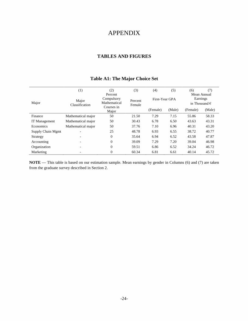
majors. Table A1 in the Appendix gives additional information on all eight majors and shows that

women are less likely to choose mathematical majors and that mathematical majors are associated

with higher earnings.

Outcomes Variables: Labor Market Outcomes: To gather data on students’ labor market

outcomes, in 2016, we sent a survey to students who graduated between September 2010 and

September 2015. From this survey, we use four outcomes: 1) yearly earnings in Euro before taxes;

2) weekly working hours; 3) job satisfaction on a 10-point scale, with 10 being “most satisfied”;

and 4) the subjective social impact of the job, ranging from -5 “very negative” to 5 “very positive,”

with 0 being “no impact.” We measured job satisfaction with the question, “How satisfied are you,

all in all, with your current work?” We measured subjective social impact with the question, “What

do you think is the social impact of your current work?” Table 1 shows average earnings to be

around 43,500 Euros per year and average working hours to be about 48 hours per week. The

average the job satisfaction is 8.1, and the average social impact of the job is 2.4 points.

The graduate survey response rate was 33 percent. We show in Appendix Table A2 that

survey response is unrelated to our peer variables of interest. To account for systematic differences

in survey response based on observable characteristics, we follow Wooldridge (2007) and

reweight all observations by the inverse of the predicted probability that we observe them in the

labor market, thus giving more weight to students that are less likely to be observed in the sample.

Empirically, this reweighting does not affect our result in any meaningful way.

Outcomes Variables: Students’ Grades and Course Evaluations: To explore mechanism that

may drive any effects on academic and labor market outcomes, we use students’ grades and their

-9-

responses to the course evaluation survey. Students’ grades are the final course grade which, in

the first-year courses we study, are exclusively based on the final exam. The business school uses

the Dutch grading scale, which ranges from 1 to 10, with 5.5 being the lowest passing grade. Table

1 shows that the average grade is 6.4. For about 5 percent of our observations, students registered

for a course, but we cannot observe their grade because they dropped out during the period.

Appendix Table A2 shows that the probability of observing a grade for a student is unrelated to

our peer variables of interest.

We measure study effort, course satisfaction, and the satisfaction with peer-to-peer

interactions with data from students’ course evaluations. The course evaluation survey is sent out

at the end of each course but before students take the final exam. From the course evaluation

survey, we obtain three variables of interest: 1) self-reported study hours per week, excluding

contact hours; 2) subjective overall course quality on a 10-point scale, with 10 being very good;

3) a quality of peer interaction index as the average of the standardized value of the two evaluation

items: “My tutorial group has functioned well” and “My fellow students helped me to better

understand the subject matter.” Table 1 shows that students report studying on average 11.8 hours

per course per week and rate the course quality on average at 7.3 on a 10-point scale.

In Column (3) of Appendix Table A2 we show that the course evaluation survey response

is unrelated to our peer variables of interest. As for the labor market outcomes, following

Wooldridge (2007), we reweight all estimates that use evaluation survey outcomes with the inverse

of the predicted probability of answering the course evaluation survey. Results are almost identical

if we do not reweight our observations.

-10-

2.3 Randomization Check

To confirm that the peer composition is random, we test whether the student “pretreatment”

characteristics of previous GPA, age, gender, and the rank of the student ID— a proxy for a

student’s tenure at the business school —systematically relate to the achievement of male and

female peers. We implement these tests by regressing peer GPA separately on each of the four

pretreatment characteristics and different sets of fixed effects. We follow Guryan, Kroft, and

Notowidigdo (2009) and additionally control for the course-level leave-out mean of GPA to

account for the mechanical relationship between own- and peer-level variables.

Table 2, in which each cell is based on a separate regression, shows the results of these

randomization tests. The first row in Column (1) for example, shows the coefficient of regressions

of own preassignment GPA on the average preassignment GPA of female peers as well as course-

year fixed effects and the course-level leave-out mean of GPA of female peers. The second, third,

and fourth observations in this column show the similar regression coefficients for the other

pretreatment characteristics. Column (2) shows results of the same regressions with the GPA of

male peers as the dependent variable. Finally, Columns (3) and (4) show versions of the same

randomization tests in which we additionally include parallel-course-year fixed effects as well as

fixed effects for time and day of the tutorial sessions.

Table 2 shows that all four pretreatment characteristics are unrelated to our peer variables

of interest. All point estimates are small and only one out of 16 coefficients of interest is

statistically significant at the 10 percent level. We confirm this result using an alternative and more

flexible randomization check, which we show in Appendix A2.

-11-

Table 2: Test for Random Assignment – Regression of Peer GPA on Student Pretreatment

Characteristics

(1) (2) (3) (4)

Dependent Variable: Std. GPA of

Female Peers

Std. GPA of Male

Peers

Std. GPA of

Female Peers

Std. GPA of Male

Peers

Std. GPA -0.0030 -0.0167 -0.0028 -0.0178*

(0.010) (0.010) (0.009) (0.010)

Female -0.0035 0.0202 -0.0003 0.0185

(0.020) (0.016) (0.020) (0.016)

Age -0.0028 -0.0071 -0.0020 -0.0067

(0.005) (0.005) (0.005) (0.005)

ID Rank 0.0000 0.0000 -0.0000 0.0000

(0.000) (0.000) (0.000) (0.000)

Observations 18,454 18,454 18,454 18,454

Course-year FE YES YES YES YES

Time, Day and Parallel-course-year FE NO NO YES YES

NOTE — Each cell in this table is estimated with a separate ordinary least squares regression including course-year

fixed effects. Following the Guryan, Kroft, and Notowidigdo (2009) correction method, we control for the leave-out

mean of the peers’ GPA at the course level in the first row. Robust standard errors using two-way clustering at the

student level and section level are in parentheses.

3. Empirical Strategy

To understand how peer achievement affects students’ specialization choices and labor market

outcomes, we estimate the following model:

𝑦𝑖𝑡+ = 𝛼1𝐹𝑒𝑚𝑎𝑙𝑒𝑖 × 𝑀𝑎𝑙𝑒𝐺𝑃𝐴̅̅ ̅̅ ̅̅ ̅̅ ̅̅ ̅̅ ̅𝑖𝑐𝑡−1 + 𝛼2𝑀𝑎𝑙𝑒𝑖 × 𝑀𝑎𝑙𝑒𝐺𝑃𝐴̅̅ ̅̅ ̅̅ ̅̅ ̅̅ ̅̅ ̅

𝑖𝑐𝑡−1+

𝛽1𝐹𝑒𝑚𝑎𝑙𝑒𝑖 × 𝐹𝑒𝑚𝑎𝑙𝑒𝐺𝑃𝐴̅̅ ̅̅ ̅̅ ̅̅ ̅̅ ̅̅ ̅̅ ̅̅𝑖𝑐𝑡−1 + 𝛽2𝑀𝑖 × 𝐹𝑒𝑚𝑎𝑙𝑒𝐺𝑃𝐴̅̅ ̅̅ ̅̅ ̅̅ ̅̅ ̅̅ ̅̅ ̅̅

𝑖𝑐𝑡−1 + 𝑋𝛾′ + 𝑢𝑖𝑐𝑡,

(1)

where 𝑦𝑖𝑡+ is the course choice, major choice, or a labor market outcome of student i at time t+,

that is, after having taken the compulsory course c at time t. We have four independent variables

of interest. 𝐹𝑒𝑚𝑎𝑙𝑒𝑖 × 𝑀𝑎𝑙𝑒𝐺𝑃𝐴̅̅ ̅̅ ̅̅ ̅̅ ̅̅ ̅̅ ̅𝑖𝑐𝑡−1 and 𝑀𝑎𝑙𝑒𝑖 × 𝑀𝑎𝑙𝑒𝐺𝑃𝐴̅̅ ̅̅ ̅̅ ̅̅ ̅̅ ̅̅ ̅

𝑖𝑐𝑡−1 are the average GPAs of all

-12-

male section peers interacted with a female and male dummy. Analogously, 𝐹𝑒𝑚𝑎𝑙𝑒𝑖 ×

𝐹𝑒𝑚𝑎𝑙𝑒𝐺𝑃𝐴̅̅ ̅̅ ̅̅ ̅̅ ̅̅ ̅̅ ̅̅ ̅̅𝑖𝑐𝑡−1 and 𝑀𝑎𝑙𝑒𝑖 × 𝐹𝑒𝑚𝑎𝑙𝑒𝐺𝑃𝐴̅̅ ̅̅ ̅̅ ̅̅ ̅̅ ̅̅ ̅̅ ̅̅

𝑖𝑐𝑡−1 are the average GPAs of all female section peers

interacted with a female and a male dummy. Each student’s GPA consists of all grades achieved

before the start of the course, which implies that neither male nor female peer GPA contain any

contemporaneous grades. 𝑋 is a vector of control variables that includes course-year fixed effects

and parallel-course-year fixed effects, which are fixed effects for the other course the students take

in the same period. We include parallel-course-year fixed effects to account for potential

nonrandom assignment due to scheduling conflicts. 𝑋 also includes students’ GPA at the start of

the course as well as indicators for student gender and nationality. 𝑢𝑖𝑐𝑡 is the error term.

The parameters of interest are 𝛼1, 𝛼2, 𝛽1, and 𝛽2.Parameter 𝛼1 captures the causal effect of

a student’s assignment to higher-GPA male peers on the outcome of interest for women, and 𝛼2

shows the equivalent effect for men. Analogously, 𝛽1 and 𝛽2 show the causal effect of a student’s

assignment to higher-GPA female peers for men and women.

One might be concerned that peer ability, not peer achievement, affects students’ choices,

and that peer GPA is a noisy measure of peer ability. In Feld and Zölitz (2017), we show that

classical measurement error in the peer variable of interest can lead to substantial overestimation

of peer effects when peer group assignment is nonrandom. When peer group assignment is random,

as in our setting, classical measurement error will bias peer effects coefficients toward zero. This

implies that because peer GPA likely measures peer ability with some degree of error, estimates

of 𝛼1, 𝛼2, 𝛽1, and 𝛽2 are likely attenuated. However, we believe that measurement error and the

resulting attenuation bias will be small because GPA is the average of all previous grades of a

student, and peer GPA consists of the average GPA over all female or male peers in a section.

-13-

To simplify the interpretation of our results, we standardize male peer GPA, female peer

GPA, course grades, the peer interaction index, job satisfaction, and subjective social impact to

have means of zero and standard deviations of one over the estimation sample. We cluster our

standard errors at the section level and student level using two-way clustering. Clustering only at

the section or only at the student level leads to same-sized or smaller standard errors.

4. Results

A. Effects on Choice of Mathematical Majors and Courses

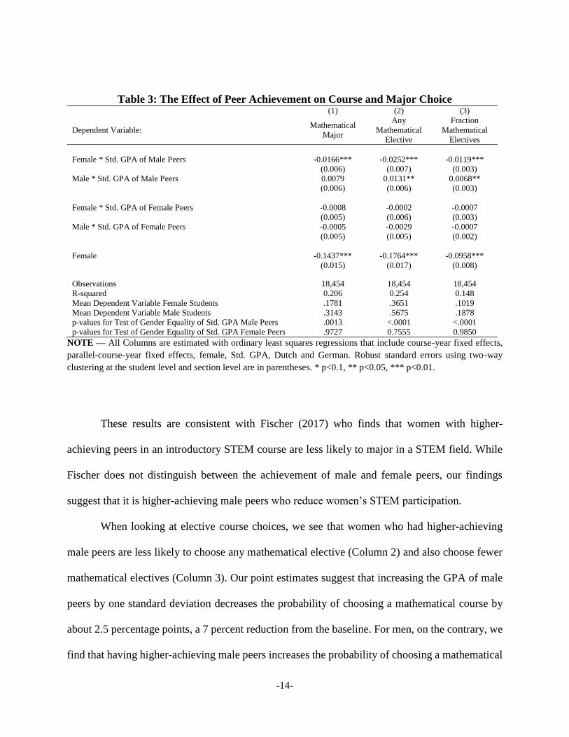
Table 3 shows that having higher-achieving male peers reduces women’s likelihood of choosing a

mathematical major. The effects size is economically significant. Having male peers with a one

standard deviation higher GPA reduces women’s probability of majoring in Finance, IT

management, or Economics by 1.7 percentage points, which is a 9 percent reduction compared to

the baseline. Men’s choice of mathematical majors is not significantly affected by having higher-

achieving male peers, with point estimates close to zero. We find no evidence that the achievement

of female peers matters for women’s or men’s major choices. These results are robust to an

alternative definition of mathematical major that includes Supply Chain Management—the only

other major that has one mathematical compulsory course.

-14-

Table 3: The Effect of Peer Achievement on Course and Major Choice (1) (2) (3)

Dependent Variable: Mathematical

Major

Any

Mathematical

Elective

Fraction

Mathematical

Electives

Female * Std. GPA of Male Peers -0.0166*** -0.0252*** -0.0119***

(0.006) (0.007) (0.003)

Male * Std. GPA of Male Peers 0.0079 0.0131** 0.0068**

(0.006) (0.006) (0.003)

Female * Std. GPA of Female Peers -0.0008 -0.0002 -0.0007

(0.005) (0.006) (0.003)

Male * Std. GPA of Female Peers -0.0005 -0.0029 -0.0007

(0.005) (0.005) (0.002)

Female -0.1437*** -0.1764*** -0.0958***

(0.015) (0.017) (0.008)

Observations 18,454 18,454 18,454

R-squared 0.206 0.254 0.148

Mean Dependent Variable Female Students .1781 .3651 .1019

Mean Dependent Variable Male Students .3143 .5675 .1878

p-values for Test of Gender Equality of Std. GPA Male Peers .0013 <.0001 <.0001

p-values for Test of Gender Equality of Std. GPA Female Peers .9727 0.7555 0.9850

NOTE — All Columns are estimated with ordinary least squares regressions that include course-year fixed effects,

parallel-course-year fixed effects, female, Std. GPA, Dutch and German. Robust standard errors using two-way

clustering at the student level and section level are in parentheses. * p<0.1, ** p<0.05, *** p<0.01.

These results are consistent with Fischer (2017) who finds that women with higher-

achieving peers in an introductory STEM course are less likely to major in a STEM field. While

Fischer does not distinguish between the achievement of male and female peers, our findings

suggest that it is higher-achieving male peers who reduce women’s STEM participation.

When looking at elective course choices, we see that women who had higher-achieving

male peers are less likely to choose any mathematical elective (Column 2) and also choose fewer

mathematical electives (Column 3). Our point estimates suggest that increasing the GPA of male

peers by one standard deviation decreases the probability of choosing a mathematical course by

about 2.5 percentage points, a 7 percent reduction from the baseline. For men, on the contrary, we

find that having higher-achieving male peers increases the probability of choosing a mathematical

-15-

course. A one standard deviation increase in male peers’ GPA increases the probability of choosing

any mathematical course by 1.3 percentage points, which is a 2.7 percent increase from the

baseline. As for major choice, we find that female peers’ GPA is not significantly related to men’s

or women’s course choices, with all point estimates being close to zero. These results suggest that

in our setting achievement of female peers does not play an important role in students’

specialization choices.

We show in Zölitz and Feld (2017) that the proportion of female peers also influences

course and major choice in the same setting. Controlling for the proportion of female peers barely

affects our estimates. Therefore, the effect of peer ability on major choice we document in this

paper is distinct from the effect of peer gender.

B. Effects on Labor Market Outcomes

Table 4 shows the estimated effects of peer achievement on a number of labor market outcomes.

We see that the effects of exposure to higher-achieving male peers persist. For women, we find

marginally statistically significant effects on earnings, which suggests that being assigned to male

peers with a one standard deviation higher GPA reduces earnings by 9 percent. The estimated

effects on working hours are economically small and not statistically significant. The most striking

result is that male peers significantly affect women’s job satisfaction and the subjective social

impact of their job. Having male peers with a one standard deviation higher GPA increases

women’s job satisfaction by 8 percent of a standard deviation and the subjective social impact of

their job by 7 percent of a standard deviation. Both estimates are highly statistically significant.

-16-

Table 4: The Impact of Peer Achievement on Labor Market Outcomes

(1) (2) (3) (4) (5)

Dependent Variable: Log Yearly

Earnings

Log

Working

Hours

Log

Hourly

Wage

Std.

Job

Satisfaction

Std.

Subjective

Social

Impact

Female * Std. GPA of Male Peers -0.0882* -0.0147 -0.0921* 0.0825*** 0.0713***

(0.049) (0.013) (0.054) (0.029) (0.017)

Male * Std. GPA of Male Peers 0.0686** 0.0004 0.0490* 0.0057 0.0117

(0.031) (0.009) (0.025) (0.023) (0.015)

Female * Std. GPA of Female Peers -0.0223 0.0036 0.0243 0.0262 -0.0144

(0.036) (0.007) (0.027) (0.026) (0.014)

Male * Std. GPA of Female Peers -0.0039 -0.0031 0.0293 0.0129 -0.0142

(0.025) (0.006) (0.022) (0.021) (0.012)

Female -0.2800*** -0.0707*** -0.2663*** -0.0608 0.0572

(0.088) (0.024) (0.086) (0.075) (0.041)

Observations 6,482 5,407 5,157 5,478 5,489

R-squared 0.109 0.136 0.063 0.025 0.700

Mean Dependent Variable Female Students 10.0562 44.9681 2.49 -.0364 .0184

Mean Dependent Variable Male Students 10.3377 49.2211 2.7204 .0366 -.1555

p-values for Test of Gender Equality of Std. GPA Male Peers .0096 .3188 .0219 .0469 .0116

p-values for Test of Gender Equality of Std. GPA Female Peers .6862 0.5297 0.8897 .7077 0.9881

NOTE — All Columns are estimated with ordinary least squares regressions that include course-year fixed effects,

parallel-course-year fixed effects, female, Std. GPA, Dutch and German. Following Wooldridge (2007), for all

specifications, we weight the observations by the inverse of the probability of observing the outcome. Robust standard

errors using two-way clustering at the student level and section level are in parentheses. * p<0.1, ** p<0.05, ***

p<0.01.

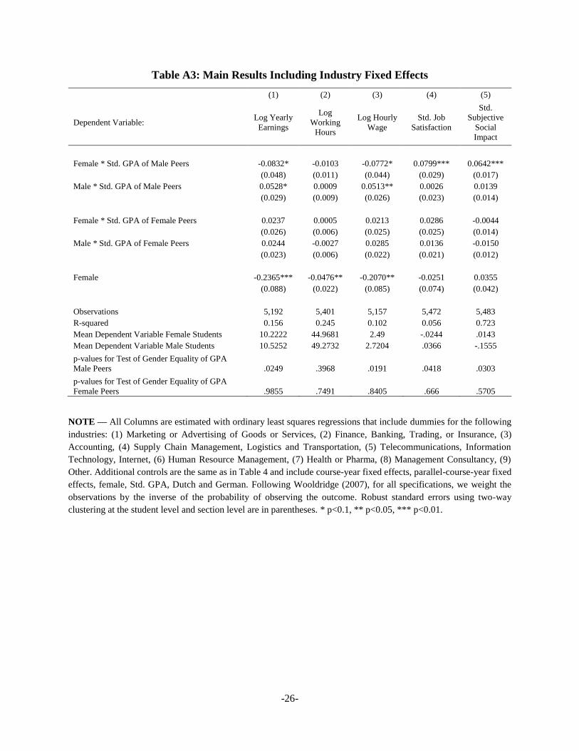
These effects might be driven by the marginal women: (1) entering different occupations,

or (2) fairing differently in the same occupation. Unfortunately, we cannot distinguish between

these two explanations empirically because we do not have precise information on graduates’

occupations such as ISCO codes. However, we do have information on nine industries that

graduates use to describe their job tasks. Controlling for industry dummies does not affect our

estimates in any meaningful way (see Table A3), which could mean that women’s occupational

choices are not affected by having higher-achieving male peers. An alternative explanation, which

-17-

we find more plausible, is that our industries are only poor proxies for occupations and the affected

women might work in different occupations within the same industry (see also Gillen, Snowberg,

and Yariv (2017) for a discussion on inference using noisy controls).

Male peers also affect men’s labor market outcomes. Having male peers with a one

standard deviation higher GPA causes men to earn 6.9 percent more per year. This point estimate

reduces to 5.3 percent and remains marginally significant when we additionally control for

industry dummies, which provides suggestive evidence that the wage effect is partly driven by the

marginal men working in different industries (see Table A3). We find no effect on working hours

and the estimated effect on hourly wage is similar in magnitude to the estimated effect on monthly

wage. We find no evidence that male peers affect men’s job satisfaction or the perceived social

impact of their job. As for major and course choice, we do not find any evidence that higher-

achieving women affect their peers labor market outcomes.

C. Mechanisms

To better understand what might drive our observed peer effects on specialization choices and

labor market outcomes, we take a closer look at how peer achievement affects students in their

first-year compulsory courses. Figure 1 shows estimates of peer achievement on students’ grades,

study effort, their evaluation of the overall course quality, and their evaluation of group interaction

in their first-year compulsory courses (see Table A4 in the Appendix for the underlying regression

estimates).

The point estimates show that higher-achieving male peers affect men’s performance and

perceptions. Men who have male peers with a one standard deviation higher GPA receive a 2

percent of a standard deviation increase in grades and increase their weekly study hours by 4

-18-

percent. They also evaluate the course quality 4 percent of a standard deviation more positively

and are 8 percent of a standard deviation more satisfied with the group interaction. In sum, men

do better with higher-achieving male peers and subsequently choose more challenging

mathematical electives. This reaction is consistent with gender differences in response to

competition (see: Niederle and Vesterlund 2007). Men seem to thrive in environments that are

more competitive due to higher-achieving peers.

Figure 1: Mechanisms—The Impact of Peer Achievement on Grades, Study Hours,

Perceived Peer Interaction, and Course Quality

NOTE — This figure is based on point estimates shown in Table A4. All Columns are estimated with ordinary least

squares regressions that include course-times-year fixed effects, parallel course fixed effects, female, Std. GPA, Dutch

and German. Following Wooldridge (2007), for all specifications except the one with grade as dependent variable, we

weight the observations by the inverse of the predicted probability of observing the outcome. The shown 90% and

95% confidence intervals are based on robust standard errors using two-way clustering at the student level and section

level.

-19-

Women’s experience in first-year courses appears to be less affected by their higher-

achieving male peers. One exception is that they evaluate the group interaction more positively.

This finding is evidence against the argument that higher-achieving men simply bully women into

choosing fewer mathematical courses and majors. We also find that women evaluate the course as

a whole more negatively if they had higher-achieving female peers, an effect that does not appear

to translate into different specialization choices.

Throughout the paper, we have seen that both men and women are less affected by their

female peers. This might be due to the discussion-based teaching style that is predominantly used

at this business school. With such a large focus on discussions, women may be less likely to speak

up and therefore be less likely to influence their peers’ specialization choices (see Jule (2001)

regarding gender differences in speaking up in the classroom).

6. Conclusion

We study how peer achievement during compulsory first-year courses affects women’s and men’s

subsequent course choices, major choices, and labor market outcomes. Our findings show that

male peers matter. Exposure to higher-achieving male peers causes women to choose fewer

mathematical courses and majors and men to choose more mathematical courses. These effects

persist. Higher-achieving male peers increase men’s earnings and decrease women’s earnings.

Most strikingly, we also find that women exposed to higher-achieving male peers end up in jobs

where they report higher job satisfaction.

Our results have potentially important implications for affirmative action policies designed

to increase women’s participation in mathematical fields. If these programs admit more women

-20-

and fewer men to selective programs, they will mechanically increase the average achievement of

male peers. Our findings suggest that these changes in the peer composition might have two types

of unintended consequences for women. First, within these programs, women may become less

likely to choose mathematical specializations. Second, when affirmative action policies are

successful at raising women’s wages, they might come—at least in the short run—at a cost to

women’s job satisfaction.

-21-

References

Astorne-Figari, Carmen, and Jamin D. Speer. 2017. “Are Changes of Major, Major Changes?

The Roles of Grades, Gender, and Preferences in College Major Switching.”

http://www.sole-jole.org/17322.pdf.

Feld, Jan, Nicolás Salamanca, and Ulf Zölitz. 2018. “Are Professors Worth It ? The Value-

Added and Costs of Tutorial Instructors.” University of Zurich, Department of Economics

Working No 293.

Feld, Jan, and Ulf Zölitz. 2017. “Understanding Peer Effects: On the Nature, Estimation, and

Channels of Peer Effects.” Journal of Labor Economics 35 (2):387–428.

https://doi.org/10.1086/689472.

Fischer, Stefanie. 2017. “The Downside of Good Peers: How Classroom Composition

Differentially Affects Men’s and Women’s STEM Persistence.” Labour Economics 46

(June). North-Holland:211–26. https://doi.org/10.1016/J.LABECO.2017.02.003.

Gillen, Ben, Erik Snowberg, and Leeat Yariv. 2017. “Experimenting with Measurement Error:

Techniques with Applications to the Caltech Cohort Study.”

Guryan, Jonathan, Kory Kroft, and Matthew J Notowidigdo. 2009. “Peer Effects in the

Workplace: Evidence from Random Groupings in Professional Golf Tournaments.”

American Economic Journal: Applied Economics 1 (4):34–68.

https://doi.org/10.1257/app.1.4.34.

Jule, Allyson. 2001. “Speaking Silence? A Study of Linguistic Space and Girls in an ESL

Classroom.” https://eric.ed.gov/?id=ED456666.

Kugler, Adriana, Catherine Tinsley, and Olga Ukhaneva. 2017. “Choice of Majors: Are Women

Really Different from Men?” Cambridge, MA. https://doi.org/10.3386/w23735.

-22-

Mengel, Friederike, Jan Sauermann, and Ulf Zölitz. 2018. “Gender Bias in Teaching

Evaluations.” Journal of the European Economic Association, February.

https://doi.org/10.1093/jeea/jvx057.

Mouganie, Pierre, and Yaojing Wang. 2017. “High Performing Peers and Female STEM Choices

in School.” SSRN Electronic Journal, October. https://doi.org/10.2139/ssrn.3049991.

Murdoch, Duncan J, Yu-Ling Tsai, and James Adcock. 2008. “P -Values Are Random

Variables.” The American Statistician 62 (3). Taylor & Francis:242–45.

https://doi.org/10.1198/000313008X332421.

Niederle, M., and L. Vesterlund. 2007. “Do Women Shy Away From Competition? Do Men

Compete Too Much?” The Quarterly Journal of Economics 122 (3). Oxford University

Press:1067–1101. https://doi.org/10.1162/qjec.122.3.1067.

OECD. 2017. Education at a Glance 2017. Education at a Glance. OECD Publishing.

https://doi.org/10.1787/eag-2017-en.

Sacerdote, Bruce. 2001. “Peer Effects with Random Assignment: Results for Dartmouth

Roommates.” The Quarterly Journal of Economics 116 (2). Oxford University Press:681–

704. https://doi.org/10.1162/00335530151144131.

———. 2014. “Experimental and Quasi-Experimental Analysis of Peer Effects: Two Steps

Forward?” Annual Review of Economics 6 (1). Annual Reviews:253–72.

https://doi.org/10.1146/annurev-economics-071813-104217.

Wooldridge, Jeffrey M. 2007. “Inverse Probability Weighted Estimation for General Missing

Data Problems.” Journal of Econometrics 141 (2):1281–1301.

https://doi.org/10.1016/j.jeconom.2007.02.002.

Zölitz, Ulf, and Jan Feld. 2017. “The Effect of Peer Gender on Major Choice.” University of

-23-

Zurich, Department of Economics Working No 270. https://doi.org/10.2139/ssrn.3071681.

-24-

APPENDIX

TABLES AND FIGURES

Table A1: The Major Choice Set

(1) (2) (3) (4) (5) (6) (7)

Major Major

Classification

Percent

Compulsory

Mathematical

Courses in

Major

Percent

Female

First-Year GPA

Mean Annual

Earnings

in Thousand €

(Female) (Male) (Female) (Male)

Finance Mathematical major 50 21.50 7.29 7.15 55.86 58.33

IT Management Mathematical major 50 30.43 6.78 6.50 43.63 43.31

Economics Mathematical major 50 37.76 7.10 6.96 40.31 43.20

Supply Chain Mgmt - 25 48.78 6.93 6.55 38.72 40.77

Strategy - 0 35.64 6.94 6.52 43.58 47.87

Accounting - 0 39.09 7.29 7.20 39.04 46.98

Organization - 0 59.51 6.86 6.52 34.24 46.72

Marketing - 0 60.34 6.81 6.61 40.14 45.72

NOTE — This table is based on our estimation sample. Mean earnings by gender in Columns (6) and (7) are taken

from the graduate survey described in Section 2.

-25-

Table A2: Testing for Attrition and Selective Survey Response

(1) (2) (3)

Grade Observed

Observed in the

Labor Market

Course Evaluation

Survey Response

Female * GPA of Male Peers -0.0026 -0.0004 -0.0081

(0.002) (0.008) (0.008)

Male * GPA of Male Peers -0.0018 -0.0055 -0.0076

(0.002) (0.007) (0.006)

Female * GPA of Female Peers -0.0021 -0.0017 -0.0038

(0.002) (0.007) (0.007)

Male * GPA of Female Peers 0.0006 -0.0095* 0.0023

(0.002) (0.005) (0.005)

Female 0.0037 -0.0122 0.0606***

(0.004) (0.019) (0.014)

Observations 18,454 14,181 18,454

R-squared 0.168 0.110 0.088

Mean Dependent Variable Female Students 0.9631 .3318 .4282

Mean Dependent Variable Male Students .9432 .3412 .3471

p-value of Test for joint Significance of Peer Variables 0.5649 0.3700 .5683

NOTE — All Columns are estimated with ordinary least squares regressions that include course-year fixed effects,

parallel-course-year fixed effects, female, Std. GPA, Dutch and German. The dependent variable in Column (1) is

equal to 1 if we observe a student’s grade and 0 otherwise. The dependent variable in Column (2) is equal to 1 if we

observe the student in the labor market, that is, if the student has answered the alumni survey and indicated that he/she

is working and 0 otherwise. The dependent variable in Column (3) is equal to 1 if the student answered the course

evaluation survey for a given course and 0 otherwise. We use the predicted value of the regressions shown in Columns

(2) and (3) to weight observations in Tables 4 and A3 following Wooldridge (2007) to give more weight to students

who we are less likely to observe. Robust standard errors using two-way clustering at the student level and section

level are in parentheses. * p<0.1, ** p<0.05, *** p<0.01.

-26-

Table A3: Main Results Including Industry Fixed Effects

(1) (2) (3) (4) (5)

Dependent Variable: Log Yearly

Earnings

Log

Working

Hours

Log Hourly

Wage

Std. Job

Satisfaction

Std.

Subjective

Social

Impact

Female * Std. GPA of Male Peers -0.0832* -0.0103 -0.0772* 0.0799*** 0.0642***

(0.048) (0.011) (0.044) (0.029) (0.017)

Male * Std. GPA of Male Peers 0.0528* 0.0009 0.0513** 0.0026 0.0139

(0.029) (0.009) (0.026) (0.023) (0.014)

Female * Std. GPA of Female Peers 0.0237 0.0005 0.0213 0.0286 -0.0044

(0.026) (0.006) (0.025) (0.025) (0.014)

Male * Std. GPA of Female Peers 0.0244 -0.0027 0.0285 0.0136 -0.0150

(0.023) (0.006) (0.022) (0.021) (0.012)

Female -0.2365*** -0.0476** -0.2070** -0.0251 0.0355

(0.088) (0.022) (0.085) (0.074) (0.042)

Observations 5,192 5,401 5,157 5,472 5,483

R-squared 0.156 0.245 0.102 0.056 0.723

Mean Dependent Variable Female Students 10.2222 44.9681 2.49 -.0244 .0143

Mean Dependent Variable Male Students 10.5252 49.2732 2.7204 .0366 -.1555

p-values for Test of Gender Equality of GPA

Male Peers .0249 .3968 .0191 .0418 .0303

p-values for Test of Gender Equality of GPA

Female Peers .9855 .7491 .8405 .666 .5705

NOTE — All Columns are estimated with ordinary least squares regressions that include dummies for the following

industries: (1) Marketing or Advertising of Goods or Services, (2) Finance, Banking, Trading, or Insurance, (3)

Accounting, (4) Supply Chain Management, Logistics and Transportation, (5) Telecommunications, Information

Technology, Internet, (6) Human Resource Management, (7) Health or Pharma, (8) Management Consultancy, (9)

Other. Additional controls are the same as in Table 4 and include course-year fixed effects, parallel-course-year fixed

effects, female, Std. GPA, Dutch and German. Following Wooldridge (2007), for all specifications, we weight the

observations by the inverse of the probability of observing the outcome. Robust standard errors using two-way

clustering at the student level and section level are in parentheses. * p<0.1, ** p<0.05, *** p<0.01.

-27-

Table A4: Mechanisms—The Impact of Peer Achievement on Grades, Study Hours and

Perceived Peer Interaction and Course Quality

(1) (2) (3) (4)

Std. Grade Log Study

Hours

Std. Overall

Course

Quality

Std. Peer

Interaction

Index

Female * Std. GPA of Male Peers -0.0039 -0.0083 -0.0046 0.0762**

(0.009) (0.014) (0.022) (0.034)

Male * Std. GPA of Male Peers 0.0195*** 0.0390*** 0.0410** 0.0772***

(0.007) (0.013) (0.019) (0.026)

Female * Std. GPA of Female Peers -0.0090 -0.0127 -0.0409** 0.0044

(0.008) (0.013) (0.018) (0.022)

Male * Std. GPA of Female Peers 0.0016 -0.0019 -0.0032 0.0121

(0.006) (0.010) (0.017) (0.019)

Female -0.0393*** 0.1199*** -0.0724** 0.0148

(0.013) (0.027) (0.029) (0.034)

Observations 17,536 6,035 6,357 4,862

R-squared 0.528 0.115 0.148 0.078

Mean Dependent Variable Female Students .1329 2.3873 -.0188 .0208

Mean Dependent Variable Male Students .0755 2.2646 .0716 -.0015

p-values for Test of Gender Equality of GPA Male Peers .0271 .0111 .0648 0.9772

p-values for Test of Gender Equality of GPA Female Peers .2541 .4899 .078 .7619

NOTE — All Columns are estimated with ordinary least squares regressions that include course-year fixed effects,

parallel-course-year fixed effects, female, Std. GPA, Dutch and German. Following Wooldridge (2007), for all

specifications, we weight the observations by the inverse of the predicted probability of observing the outcome. Robust

standard errors using two-way clustering at the student level and section level are in parentheses. * p<0.1, ** p<0.05,

*** p<0.01.

-28-

Figure A1: Distribution of the Mean GPA of Male and Female Section Peers

-29-

APPENDIX

A1 Data Restrictions

In this paper, we use the same estimation sample as in Zölitz and Feld (2017) with the exception

that we additionally have to exclude sections with fewer than two female or fewer than two male

students because in these sections, one of our core independent variables, either the male peer GPA

or the female peer GPA, is missing.

Our sample period comprises the academic years 2009/2010 through 2014/2015. We derive

our estimation sample in two steps. First, we exclude a number of observations from our estimation

sample because they represent exceptions from the standard section assignment procedure. These

exceptions are the same as documented in as in Feld, Salamanca, and Zölitz (2017), who use data

from the same environment and sample period. Second, we further limit our estimation sample to

the two main bachelor’s programs offered at the business school beginning in the academic years

2009/2010 until 2011/2012 because we can follow these cohorts from their first until their last

bachelor’s year and observe their major choices.

Below we list the observations we exclude due to exceptions to the scheduling procedure.

• We exclude eight courses in which the course coordinator or other education staff actively

influenced the section composition. One course coordinator requested to balance student gender

across sections. The business school’s scheduling department informed us about these courses.

• We exclude 21 sections from the analysis that consisted mainly of students who registered late

for the course. Before April 2014, the business school reserved one or two slots per section for

students that registered late. In exceptional cases in which the number of late registration

students substantially exceeded the number of empty spots, new sections were created that

-30-

mainly comprised late registering students. The business school abolished the late registration

policy in April 2014.

• We exclude 46 repeater sections from the analysis. One course coordinator explicitly requests

that students who failed his/her courses in the previous year be assigned to special repeater

sections.

• We exclude 17 tutorial groups that consisted mainly of students from a special research-based

program. For some courses, students in this program were assigned together to separate tutorial

groups with a more-experienced teacher.

• We exclude 95 part-time MBA students because these students are typically scheduled for

special evening classes with only part-time students.

• We exclude 4,274 student-year observations for students who were repeating courses. These

students follow a different attendance criterion and are graded under different standards.

• We exclude all observations of the first-year and the first-period students. For these

observations, we have no measure of previous performance of the student at the business school,

an essential variable in our analyses.

• We exclude all observations from the first teaching period of 2009, which is the first period in

our data set, for the same reasons outlined above.

• We exclude 1,229 student-year observations from sections that take place after 6:30 p.m.

because prior to the Fall 2015 semester, students could opt out of evening education, which

makes the student assignment to these sections potentially nonrandom.

-31-

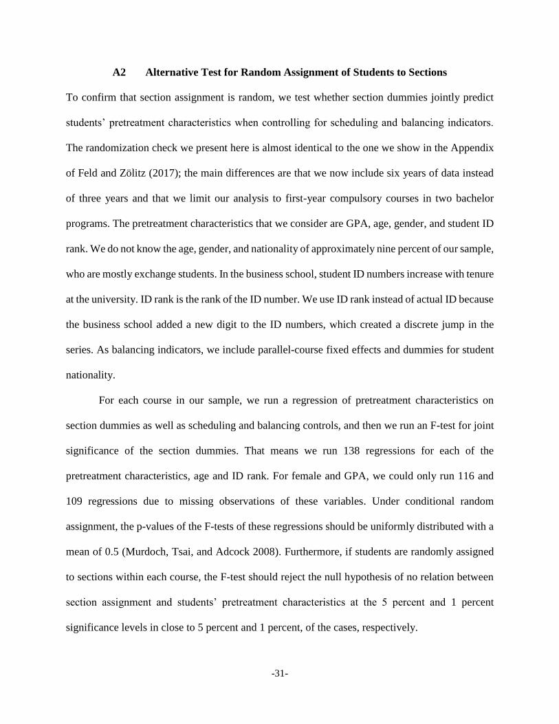
A2 Alternative Test for Random Assignment of Students to Sections

To confirm that section assignment is random, we test whether section dummies jointly predict

students’ pretreatment characteristics when controlling for scheduling and balancing indicators.

The randomization check we present here is almost identical to the one we show in the Appendix

of Feld and Zölitz (2017); the main differences are that we now include six years of data instead

of three years and that we limit our analysis to first-year compulsory courses in two bachelor

programs. The pretreatment characteristics that we consider are GPA, age, gender, and student ID

rank. We do not know the age, gender, and nationality of approximately nine percent of our sample,

who are mostly exchange students. In the business school, student ID numbers increase with tenure

at the university. ID rank is the rank of the ID number. We use ID rank instead of actual ID because

the business school added a new digit to the ID numbers, which created a discrete jump in the

series. As balancing indicators, we include parallel-course fixed effects and dummies for student

nationality.

For each course in our sample, we run a regression of pretreatment characteristics on

section dummies as well as scheduling and balancing controls, and then we run an F-test for joint

significance of the section dummies. That means we run 138 regressions for each of the

pretreatment characteristics, age and ID rank. For female and GPA, we could only run 116 and

109 regressions due to missing observations of these variables. Under conditional random

assignment, the p-values of the F-tests of these regressions should be uniformly distributed with a

mean of 0.5 (Murdoch, Tsai, and Adcock 2008). Furthermore, if students are randomly assigned

to sections within each course, the F-test should reject the null hypothesis of no relation between

section assignment and students’ pretreatment characteristics at the 5 percent and 1 percent

significance levels in close to 5 percent and 1 percent, of the cases, respectively.

-32-

Table A5 shows the number of cases in which the F-test actually rejected the null

hypothesis at the respective levels. Column (1) shows the total number of course-level regressions

for each pretreatment characteristic. Columns (2) to (5) shows the actual rejection rates at the 5

percent and 1 percent levels respectively. All rejection rates are close to the expected rejection

rates under random assignment. Column (6) shows that the averages of the p-values of the F-tests

for each characteristic are close to 0.5. Figure A2 confirms that the p-values are roughly uniformly

distributed. All together, we present additional evidence that section assignment in our estimation

sample is random, conditional on scheduling and balancing indicators.

Table A5: Alternative Randomization Check

Dependent Variable Number significant at: Percent significant at: Total Number

of Courses

Mean of p-

value

5% 1% 0.1% 5% 1% 0.1%

Female 4 0 0 0.034 0.000 0.000 116 0.5786

GPA 5 2 0 0.046 0.018 0.000 109 0.4795

Age 8 3 0 0.058 0.022 0.000 138 0.4793

ID rank 3 0 0 0.022 0.000 0.000 138 0.5534

NOTE — This table is based on separate OLS regressions with female, GPA, age, and ID rank as dependent variables.

The explanatory variables are a set of section dummies, dummies for the other parallel course taken at the same time,

and dummies for day and time of the sessions, German, and Dutch.

-33-

Figure A2: Alternative Randomization Check - Distributions of p-values

NOTE — These are histograms with p-values from all the regressions reported in Table A1. The vertical line in

each histogram shows the 5 percent significance level.

0

.02

.04

.06

.08

Fra

ction

0 .1 .2 .3 .4 .5 .6 .7 .8 .9 1p-values

Female

0

.02

.04

.06

.08

Fra

ction

0 .1 .2 .3 .4 .5 .6 .7 .8 .9 1p-values

GPA

0

.02

.04

.06

.08

Fra

ction

0 .1 .2 .3 .4 .5 .6 .7 .8 .9 1p-values

AGE

0

.02

.04

.06

.08

Fra

ction

0 .1 .2 .3 .4 .5 .6 .7 .8 .9 1p-values

ID rank