Iterative Decoding of Turbo Product Codes (TPCs)...

Iterative Decoding of Turbo Product Codes (TPCs)

Using the Chase-Pyndiah Turbo Decoder

Muath Ghazi Abdel Qader Ghnimat

Submitted to the

Institute of Graduate Studies and Research

in partial fulfilment of the requirements for the degree of

Master of Science

in

Electrical and Electronic Engineering

Eastern Mediterranean University

February 2017

Gazimağusa, North Cyprus

ii

Approval of the Institute of Graduate Studies and Research

__________________________

Prof. Dr. Mustafa Tümer

Director

I certify that this thesis satisfies all the requirements as a thesis for the degree of

Master of Science in Electrical and Electronic Engineering.

_________________________________________________

Prof. Dr. Hasan Demirel

Chair, Department of Electrical and Electronic Engineering

We certify that we have read this thesis and that in our opinion it is fully adequate in

scope and quality as a thesis for the degree of Master of Science in Electrical and

Electronic Engineering.

________________________________

Prof. Dr. Erhan A. İnce

Supervisor

Examining Committee

1. Prof. Dr. Hasan Amca __________________________________

2. Prof. Dr. Hasan Demirel __________________________________

3. Prof. Dr. Erhan A. İnce __________________________________

iii

ABSTRACT

The ground breaking error correction codes that could achieve low bit error rates

(near Shannon’s limit) were Turbo Codes (TCs) introduced by Berrou, Glavieux in

1993. The encoders for these outstanding codes were created by parallel

concatenation of two recursive systematic convolutional codes separated by an

interleaver. For decoding TCs Log-MAP algorithm could be used due to its gain in

computational speed and improvement in precision. The only problem with turbo

coding and decoding is that, the choice of interleaver for the encoder may cause an

error floor due to their inherent poor distance properties.

Turbo product codes (TPCs) are powerful linear block codes formed by combining

more than one simple linear block codes. They classify under serially concatenated

codes however unlike TCs they do not rely on an interleaver and hence they have no

error floor problem. TPCs which date as early as 1954, are multi-dimensional codes

that are constructed by two or more linear block codes also known as component

codes. The product code is obtained by placing (k1k2) information bits in an array

with k1 rows and k2 columns. Important parameters of a product code are the length

of the codeword (n), the length of the information (k) and the minimum distance (d).

Turbo product decoding is possible using either hard or soft decoding. In hard

decision decoding, the input must be a binary sequence, whereas in soft decision

decoding the values are immediately processed by the decoder to gauge a code

sequence. A SISO decoder can be utilized to generate the soft decision decoder

outputs. Some of the soft decoding algorithms include: the maximum a posteriori

probability (MAP) algorithm, Chase-Pyndiah iterative decoder, symbol based MAP

iv

algorithm, the Soft Output Viterbi Algorithm, sliding‐window based MAP decoder,

and the forward recursion based MAP decoder. The work presented in this thesis

presents the bit-error-rate (BER) versus signal-to-noise-ratio (SNRdB) for soft

decision (SD) decoding. The modulation type is BPSK and encoded symbols are

transmitted over AWGN and Rayleigh fading channels. For SD the Chase-Pyndiah

decoding algorithm was simulated to lower the bit error rate from iteration to

iteration. We assumed an information array of (4×4) and the coded array had

dimensions (7×7) for the first code, and an information array of (11×11) and the

coded array had dimensions (15×15) for the second one. BER results were obtained

as ensemble average of many runs (repetitions).

Simulation results indicate that the SD with Chase-Pyndiah algorithm provides

nearly 1.1dB lower BER in comparison to the uncoded BPSK over AWGN channel

for (7,4)2 and 2.6dB when using the (15,11)

2 at target BER of 10

-3. For flat fading

Rayleigh channel, the simulation achieved at around 18dB SNR value for the (7,4)2

TPC and at 15dB for the (15,11)2

at target BER of 10-3

, whereas the uncoded BPSK

could achieve the same target BER beyond 20dB.

Keywords: Turbo product codes, Iterative decoding, Chase-Pyndiah algorithm.

v

ÖZ

Shannon sınırının yakınında düşük bit hata oranlarına ulaşabilen hata düzeltme

kodları, 1993 yılında Berrou ve Glavieux tarafından önerilen Turbo Kodlar (TC) idi.

Bu seçkin kodlar için kodlayıcılar, bir serpiştirici ile ayrılmış iki ardışık sistematik

evrişimsel kodun paralel birleştirilmesi ile oluşturulmaktaydı. TC'lerin şifresini

çözmek için hesaplama hızındaki kazanç ve hassaslığı artırması nedeniyle Log-MAP

algoritması kullanılabilir. Turbo kodlama ve kod çözme ile ilgili tek problem,

kodlayıcıdaki serpiştirici seçimine bağlı olarak, serpiştiricinin içsel zayıf mesafe

özelliklerinden dolayı bir hata zeminine neden olabilmesidir.

Turbo çarpım kodları (TPC'ler) birden fazla basit, doğrusal blok kodunu birleştirerek

oluşturulan güçlü doğrusal blok kodlarıdır. TPCler sıralı olarak birleştirilmiş kodlar

altında sınıflandırırlar, ancak TC'lerin aksine bir kodlayıcıya dayanmazlar ve

dolayısıyla hata zemini problemleri yoktur. 1954 yılına kadar uzanan TPC'ler,

bileşen kodları olarak da bilinen iki veya daha fazla doğrusal blok kodla

oluşturulmuş çok boyutlu kodlardır. Çarpım kodu, (k1×k2) bilgi bitlerini k1 satır ve k2

sütunları içeren bir diziye yerleştirerek elde edilir. Bir çarpım kodunun önemli

parametreleri, bilginin uzunluğu (n), kod sözcüğünün uzunluğu (k) ve en ufak mesafe

(d) dir. Turbo çarpım kodlarının çözümü, sert veya yumuşak kod çözme yöntemleri

kullanarak gerçekleştirilebilir. Sert karar tabanlı çözme işleminde girdi ikili bir dizi

olmalı, yumuşak kararlı çözücülerde ise değerler bir kod sırasını ölçmek için kod

çözücü tarafından hemen işlenmelidir. Yumuşak kararlı kod çözücünün çıktılarını

üretmek için bir SISO kod çözücü kullanılabilir. Yumuşak kod çözme

algoritmalarından bazıları şunlardır: en büyük sonsal olasılık (MAP) algoritması,

vi

Chase-Pyndiah iteratif kod çözücüsü, sembol tabanlı MAP algoritması, yumuşak

çıkışlı Viterbi algoritması, kayan-pencere tabanlı MAP dekoder ve ileri yineleme

tabanlı MAP dekoder. Bu çalışmada, yumuşak kararlı (SD) bir kod çözücü için farklı

sinyal / gürültü oranlarında (SNRs) bit hata oranları (BERs) hesaplanmıştır.

Modülasyon tipi olarak BPSK kullanılmış ve kodlanmış sembollerin AWGN ve düz

sönümlemeli Rayleigh kanalları üzerinden iletimi yapılmıştır. Benzetimler esnasında

farklı iterasyonlardaki bit-hata-oranını düşürebilmek için Chase-Pyndiah şifre çözme

algoritması kullanılmıştır. Bilgi dizisinin (4×4) olduğu ilk kod için kodlanmış dizinin

boyutları (7×7) ve bilgi dizisinin (11×11) olduğu ikinci kod için kodlanmış dizinin

boyutu (15×15) idi. Bit-hata-oranı sonuçları, çok sayıdaki benzetimin toplam

ortalaması olarak elde edilmiştir.

Simülasyon sonuçları göstermiştir ki iteratif Chase-Pyndiah şifre çözme algoritması

kullanılıp, AWGN kanalı üzerinde (7,4)2 TPC kodlu veri iletimi gerçekleştirildiğinde

10-3

hedef BER şifrelenmemiş BPSKye göre 1.1dB daha önce sağlanmıştır. (15,11)2

kodlu veri iletimi için ise bu değer 2.6dB daha önce sağlanabilmektedir. Düz

sönümlemeli Rayleigh kanalı üzerinde 10-3

hedef BER (7,4)2

ve (15,11)2

TPC kodlu

veri iletimleri için sırası ile 18dB ve 15dB de elde edilirken kodlanmamış BPSK aynı

hedef bit-hata-oranını ancak 20dBden sonar sağlayabilmektedir.

Anahtar Kelimeler: Turbo çarpım kodları, iteratif kod çözücüsü, Chase-Pyndiah

algoritması.

vii

DEDICATION

To My Family

viii

ACKNOWLEDGMENT

I would like to thank my supervisor Prof. Dr. Erhan A. İnce for his inspiration and

continuous feedback. Without his careful guidance this study would not have been

successively completed.

A special thanks to Dr. Mahmoud Nazzal for having discussions with me from time

to time and showing me how to use MATLAB efficiently. Great thanks to all of my

friends for their presence, as it enhanced my motivation by making me feel at home.

Finally, I especially wish to thank my lovely mother, father, brothers, sisters and

uncles who have provided me with immeasurable support and encouragement during

all these years.

ix

TABLE OF CONTENTS

ABSTRACT ………………………………………………………………………...iii

ÖZ………………………………………….………………………………………...v

DEDICATION ……………………….……………………………………………..vii

ACKNOWLEDGMENT …………………………………………………………..viii

LIST OF FIGURES …………………………………………………………….….. xi

LIST OF ABBREVIATIONS ……………….…………….……………………... xiii

1 INTRODUCTION .................................................................................................... 1

1.1 Literature Review .............................................................................................. 2

1.2 Thesis Outline .................................................................................................... 4

2 TURBO PRODUCT ENCODER .............................................................................. 5

2.1 Concatenated codes ........................................................................................... 6

2.2 Turbo Product Encoder ...................................................................................... 8

3 TURBO PRODUCT DECODER: STRUCTURE AND ALGORITHMS ............. 11

3.1 Hard Input Hard Output Decoding .................................................................. 11

3.2 Soft Input Soft Output Decoding ..................................................................... 12

3.3 Structure of a Soft Input Soft Output Decoder ................................................ 12

3.4 The Maximum a Posteriori Probability (MAP) Algorithm ............................. 14

4 CHASE DECODERS AND CHASE-PYNDIAH ALGORITHM ......................... 17

4.1 Introduction ..................................................................................................... 17

4.2 Type-I Algorithm ............................................................................................. 18

4.3 Type-II Algorithm ........................................................................................... 19

4.4 Type-III Algorithm .......................................................................................... 19

4.5 Chase-Pyndiah Algorithm ............................................................................... 19

x

5 SIMULATION BASED BER PERFORMANCE .................................................. 25

5.1 Simulation results over AWGN Channel ........................................................ 26

5.2 Simulation results over Rayleigh Fading Channel .......................................... 28

6 CONCLUSION AND FUTURE WORKS ............................................................. 32

6.1 Conclusion ....................................................................................................... 32

6.2 Future work ..................................................................................................... 33

REFERENCES…………………………..………………………………………….35

APPENDIX ........................................................................................................... 39

Appendix A: MATLAB implementation of Chase-Pyndiah Decoder ................. 40

xi

LIST OF FIGURES

Figure ‎2.1: Concatenated Codes. ................................................................................. 7

Figure ‎2.2: Concatenated Encoder and Decoder with Interleaver. .............................. 7

Figure 2.3: The construction structure of TPCs (P = C1 × C

2). ................................... 8

Figure ‎2.4: Placing Information Bits in a (k1 × k2) Array. ........................................... 9

Figure 2.5: Encoding the k2 Rows to produce n1 Columns using C1.. ......................... 9

Figure ‎2.6: Encoding the n1 Columns to produce n2 Rows using C2. ........................ 10

Figure ‎2.7: Construction of (7,4)2

TPC…………………………………….………..10

Figure 3.1: Turbo Product Decoder Component Decoder ......................................... 13

Figure ‎3.2: Architecture of Turbo Product Decoder. ................................................. 14

Figure ‎4.1: Geometric Sketch for decoding algorithm. ............................................. 18

Figure ‎4.2: Two-Dimensional TPC Iterative Decoding Process. ............................... 21

Figure ‎5.1: Transmission over the AWGN Channel. ................................................. 26

Figure ‎5.2: Bit error rate performance for Chase-Pyndiah decoder for information

transmitted over the AWGN channel after (7,4)2 encoding [ BPSK modulation,

Repetition = 7000, number of least reliable bits (p)=4]. ............................................ 27

Figure ‎5.3: Bit error rate performance for Chase-Pyndiah decoding of information

transmitted over the AWGN channel after (15,11)2 encoding [Code Rate ≈ 0.54,

BPSK modulation , Repetition=1000, number of least reliable bits (p) =10]. ........... 28

Figure ‎5.4: Simulation Model for transmission over the Rayleigh fading channel. .. 29

Figure ‎5.5: Frequency response for a flat fading Rayleigh channel. ......................... 30


transmitted over the Rayleigh fading channel using (7,4)2

encoding [Code Rate ≈

0.33, BPSK modulation , Repetition=1000, number of least reliable bits (p) =4]. .... 31

xii


transmitted over the Rayleigh fading channel using (15,11)2 encoding [Code Rate ≈

0.54, BPSK modulation , Repetition=1000, number of least reliable bits (p) =10]. .. 31

Figure ‎6.1: An case of 4 least reliable value.……….……..………...………..……..33

xiii

LIST OF ABBREVIATIONS

TCs Turbo Codes

TPCs Turbo product codes

SISO Soft Input Soft Output

MAP Maximum A Posteriori Probability

BER Bit Error Rate

SNR Signal to Noise Ratio

SD Soft Decision

ECC Error Correcting Coding

AWGN Additive White Gaussian Noise

LDPC Low Density Parity Check Codes

LAN Local Area Network

HD Hard Decision

FEC Forward Error Correction

HIHO Hard Input Hard Output

SDD Soft Decision Decoding

xiv

LLR Log Likelihood Ratio

BPSK Binary Phase Shift keying

CTC Convolutional Turbo Code

LOS Line of Sigh

GA Genetic Algorithm

PSO Particle Swarm Optimization

https://www.viasat.com/technologies/convolutional-turbo-codes-ctcs

1

Chapter 1

1. INTRODUCTION

In the nearby past years, there was a quick development in wireless mobile

communication systems because the demand for applications that uses wireless

mobile communication systems had been increasing very quickly. The major goal in

communication systems are minimize the error probability by design an efficient

systems of power and bandwidth resources, while reducing the complexity in order

to save the time and reduce the cost .

Communication engineering attempt to transmit the information bits from the source

to the destination via a channel with high reliability. Indeed, this is a difficult task

since there are many factors to cause faults. Detecting and correcting errors is

important while sending information bits. If we cannot detect the occurred errors and

so we cannot correct them, the received information bits at the destination site will be

differ from the original source information bits. These defect in the data sequence

what the communication engineers try to reduce.

The information bits include any coding scheme matched to the nature of the data.

The error correcting coding (ECC) encoder takes data bits as input from the source

and adds redundant bits as additive white Gaussian noise (AWGN), then moves to

the process of modulating a signal, sending it over a communication channel,

2

demodulating it, and finally decoding the data bits to get the original information

bits.

1.1 Literature Review

Reliability measured by the ability of errors correction and received information bits

at receiver without errors or with a little percentage of errors, so it considered as one

of the major aims when sending information bits over any medium. As long as the

channel capacity is greater than the transmission rate, the reliability is possible even

over channels with noise (Cover & Thomas, 1991). Claude Shannon shows this

outcome for an AWGN channel in 1948, is known as the Shannon's Theorem or

noisy channel coding theorem (Shannon, 1948).

Channel coding is used to protect the information bits from interference and noise

and minimize the number of bit errors. The main idea is the transmitter encodes the

information bit by adding redundant bits by using an ECC. The scientist Richard

Hamming pioneered this field in the 1940s and created the first ECC in 1950 and

called it the Hamming (7, 4) code.

This redundant bit allows detecting and correcting the bit errors at the received

information bits. The cost of using channel coding to protect the information is an

expansion in bandwidth or a reduction in data rate.

There are two principle sorts of channel codes, in particular block codes (also called

algebraic codes) and convolutional codes (Lin & Costello, 1983) (Wicker, 1995).

There are numerous contrasts between these two distinct sorts of coding systems.

This difference was fundamentally taking into account three perceptions. Firstly,

block codes are proper for protecting blocks of information bits independent one

https://en.wikipedia.org/wiki/Hamming_(7,4)_code

3

from the other whereas convolutional codes are suitable for protecting continuous

streams of information bits. Secondly, the code rates of block codes are close to

unity, while the code rates of convolutional codes are lower. Finally, block code

decoding is sort of the hard input decoding and using soft input decoding for

convolutional codes.

Presently, these differences are setting out toward blur. Convolutional codes can

undoubtedly be fitting to encode blocks and soft inputs decoders have been accepted

in block codes. Block code can be minimizing values of code rates to become equal

with convolutional codes.

The requirement of modern coding is concatenated structures. The concatenated

structures are using a few basic encoders and whose decoding is performed by

iterated entries in the related decoders. The sort of iterative processing was opened

by Turbo codes (1993) and from that point numerous concatenated structures

depended on iterative decoding have been rediscovered (or envisioned). Some of

these include turbo codes (TCs) and, low-density parity-check codes (LDPC). Each

of these codes have been received in universal standards, and comprehension their

coding forms and their decoding algorithms is a premise sufficiently wide to handle

whatever other norms of disseminated coding and of related iterative decoding.

In this thesis, one of the linear block code types, called Block turbo codes also

known as a Turbo product codes (TPCs) is presented. TPCs which are obtained by

serial concatenation of simpler block codes were first proposed by Elias in 1954

(Elias, 1954).

4

1.2 Thesis Outline

Chapter 2 provides a brief introduction to the idea behind Turbo Product Codes

(TPCs) and provides details on how the encoder for TPCs operates. It also explains

how to calculate the rate of the TPC given the two constituent codes.

Chapter 3 presents the general structure for a soft input soft output (SISO) iterative

decoder that can be used to decode TPCs, and also explains in detail the Maximum a

Posteriori Probability (MAP) algorithm.

Chapter 4 points out the reason for choosing the Chase-Pyndiah iterative decoder for

the decoding of TPCs and after explaining the three versions of the Chase algorithms

provides full details on how to implement the Chase-Pyndiah decoder.

Chapter 5 studies the performance of TPCs through computer simulation using the

MATLAB platform. Additive White Gaussian and Rayleigh fading channels are

realized and information encoded using various TPCs are transmitted over the

channels and retrieved at the receiver side using a Chase-Pyndiah decoder.

Chapter 6 concludes the thesis and gives some directions for future work.

Finally, the Appendix-A includes the 9 MATLAB functions developed while

implementing the Chase-Pyndiah decoder.

5

Chapter 2

2. TURBO PRODUCT ENCODER

Turbo coding was first presented during 1993 by Claude Berrou. Until that time,

scientists believed that it would be impossible to attain BER performances near

Shannon’s bound without vast complexity.

Turbo codes are obtained by two (or more) constituent codes which are also known

as serial or parallel concatenation. There are two known forms of constituent codes:

(i) block codes and (ii) convolutional codes. Turbo Product Codes (TPCs) which are

also known as Block Turbo Codes (BTCs) is a variation on the conventional Turbo

Coding but TPC encoding/decoding does not have an error floor problem as with

TCs.

Turbo product codes are mainly used in mobile communications, wireless Local

Area Networks (LAN), wireless internet access and satellite communications (M,

Gao, & Vilaipornawai, 2002).

The ideas below constitute the base of turbo product codes:

1. Block codes are employed as an alternative of generally used systematic or

non-systematic convolutional codes.

2. SISO decoding (SDDs) is employed as an alternative to HDDs.

6

3. Construct a long block code with moderate decoding complexity by

combining shorter codes. Uses iterative decoding.

2.1 Concatenated codes

In 1954, Elias presented concatenated codes which assist in improving the authority

of FEC (Forward Error Correction) codes. The theory supplies the production of

outer encoder that contributes to a new encoder. The inner encoder is recognized as

the concluding encoder prior to the channel. The consequential composite code is

evidently more intricate than any of the character codes. On the other hand it can

willingly be decoded: we basically pertain each of the factor decoders in turn, from

the internal to the outer (Burr, 2001).

This straight forward system suffers a down side which is called error propagation. If

a decoding error occurs in a codeword, it frequently consequences in a number of

data error. When these are approved on to the subsequent decoder they may over

power the capability of that code to correct the errors. The presentation of the outer

decoder may be enhanced if these errors were circulated between a numbers of

detached codeword. This is achieved via an interleaver/de-interleaver.

This interleaver contains of a two-dimensional array. Then, the data is interpreted all

alongside its rows. After the array is filled, the information is interpreted out by

columns, thus changing the arrangement of the information.

7

Figure 2.1: Concatenated Codes (Burr, 2001).

Interleaver could be positioned among the inner and outer encoders of a concatenated

code that practices two element codes, the de-interleaver linking the outer and inner

decoders in the recipient, as you can see in Figure 2.2. Afterwards, only if the rows

of the interleaver are at the slightest provided that the outer codeword’s, plus the

columns are at the slightest on condition that the inner data blocks, every information

bit of an inner codeword fall into a singular outer codeword. Therefore, so long as

the outer code is capable of correcting no less than one error, it can at all times

handle with particular decoding errors in the inner code.

Figure 2.2: Concatenated Encoder and Decoder with Interleaver (Burr, 2001)

8

2.2 Turbo Product Encoder

TPCs are obtained by serial concatenation of linear block codes (MacWilliams &

Sloane, 1978). The idea is to construct simple yet powerful codes with large

minimum Hamming distance.

Figure 2.3: The construction structure of TPCs (P = C1 × C

2) (Al Muaini, AlDweik,

& AlQutayri, 2011).

Consider we have two systematic linear block codes C1 with parameters (n1, k1, d

(1)

min ) and C2

with parameters (n2 , k2 , d(2)

min ), where ni , ki and di , (i=1,2) indicates

to codeword length, number of information bits, and minimum Hamming distance,

respectively. The block codes C1 and C

2 are named component or constituent codes

and the resulting product code P can be represented as (n1n2, k1k2, d (1)

min d (2)

min).

As shown in Figure 2.3, the turbo product code is obtained as follows (Al Muaini,

AlDweik, & AlQutayri, 2011) :

4. (k1 × k2) data is placed in an array of k2 rows and k1 columns.

9

5. encode the k2 rows using C1.

6. encode the n1 columns using C2

to produce n2 rows.

The code rate R for the constructed product code P would be RP = R1 × R2, where Ri

is the code rate of code Ci and the correcting capabilities of turbo product code is

denoted by t = [(dmin -1) / 2]. Thus, we can shape much extended block codes with

huge MHD by assembly short codes that have slight MHD.

Figure 2.4: Placing Information Bits in a (k1 × k2) Array.

Figure 2.5: Encoding the k2 Rows to produce n1 Columns using C1.

10

Figure 2.6: Encoding the n1 Columns to produce n2 Rows using C2.

Note that the (n2 - k2) final rows are codewords of C1 and (n1 – k1) final columns of

the array are codewords of C2 (Prasad & Nee, 2004). Figure 2.7 shows the

construction of (7,4)2 TPC and is an extract from (He & Ching, 2007).

Figure 2.7: Construction of (7,4)2

TPC (He & Ching, 2007).

Transmission encoded using TPCs are decoded using sequential “columns/rows”

decoding to lower the decoding complexity. To attain better performance than the

HDDs, we have to use SD of the constituent codes.

11

Chapter 3

3. TURBO PRODUCT DECODER: STRUCTURE AND

ALGORITHMS

In this chapter we present algorithms for decoding Turbo Product Codes (TPCs)

when the inputs are either hard or soft data. We first provide the general structure for

a soft input soft output (SISO) iterative decoder and later explain in detail the

Maximum a Posteriori Probability (MAP) algorithm.

3.1 Hard Input Hard Output Decoding

For a hard input hard output (HIHO) system, the output of the demodulator needs to

be converted to binary. The output ( ) where * + can be

calculated using:

, ( ) - (3.1)

Where R denotes the corresponding received sequence.

Once R has been computed, the maximum likelihood decoding (MLD) can be

achieved searching for the codeword D that gives the minimum Hamming distance to

H:

| | | | , - (3.2)

Unfortunately, the complexity of the search for D will become high for large n values

and the solution is to partition H into two separate vectors that can be decoded

12

independently. For independent decoding of the individual parts row/column

decoding can be used. In the first half iteration n1 rows will be decoded and in the

following half iteration n2 columns will be decoded. For example, the Berlekamp-

Massey algorithm described in (Berrou, Codes and Turbo Codes, 2010) can be used

for HIHO decoding.

3.2 Soft Input Soft Output Decoding

For the soft input soft output (SISO) decoding maximum likelihood decoding is

achieved by searching for the codeword D that minimizes the distance between D

and R. Similar to the HIHO case explained in section 3.1, R is partitioned into

smaller row/column vectors. Afterwards, each vector (row/column) is decoded using

soft decision decoding (SDD). One efficient SDD algorithm suggested for decoding

of TPCs was first proposed in 1994 by R. Pyndiah (Pyndiah, Alain, Picart, & Jacq,

1994). This iterative decoder which is based on the Chase II algorithm (Chase, 1972)

is known as Chase-Pyndiah iterative decoder. Each iteration of a Chase-Pyndiah

decoder is composed of two half iterations. In the first half iteration the rows of the

product code are decoded first. Similarly in the second half-iteration the columns are

decoded. To reduce the bit error probability the algorithm will take multiple

iterations. According to Kim there is a fine balance between performance and

complexity of decoder. Therefore, the implementation of SDD is a very important

issue.

3.3 Structure of a Soft Input Soft Output Decoder

The component decoder for a turbo product code is as depicted in Figure 3.1. Given

the information received from the channel (Ri) the SISO decoder computes the soft

output (LLRi) during the first half-iteration. Since for the remaining half-iterations

the demodulator does not provide actual soft information the algorithm has to

13

compute extrinsic information (Ei) from Ri and LLRi by multiplying LLRi by

and then subtracting Ri from the answer. Note that is a weight factor.

Figure 3.1: Turbo Product Decoder Component Decoder (Kim, 2015).

The algorithms have high complexity are Log-MAP algorithm or optimal MAP

algorithm. Suboptimal variants like Max-log-MAP algorithm and Log-MAP

algorithm are utilized in practice. The SOVA has low complexity so it considered as

desirable algorithm. However, the Max-log-MAP algorithm has better performance

than SOVA. The Log-MAP decoding scheme is the modified version of the MAP

decoding scheme and is computationally less complex than the original MAP

decoding algorithm (Kim, 2015).

Trellis of block codes can be represented, which allows us to implement ML or MAP

decoding, but the complexity increments whenever the codeword length increments.

So is appropriate for column or row codes or in general, for any short length codes.

The turbo product decoder in the receiver utilizes soft decision data bits sequence.

Figure 3.2 represents the architecture of turbo product decoder.

14

Figure 3.2: Architecture of Turbo Product Decoder (Kim, 2015).

3.4 The Maximum a Posteriori Probability (MAP) Algorithm

The reduction of the bit error rate in the decoding process is considered the main

objective of MAP algorithm. Hence, in the wake of accepting the data out of the

channel, the decoder set the most probable input bits, depends on the received bits.

Since the input bits are binary, it is customary to shape a log-likelihood ratio (LLR)

(Vucetic & Yuan, 2000) and base the bit gauges on correlations taking into account

size of the probability proportion to a threshold. The ratio of log-likelihood for the

input bits indexed at time t is known as

( ) ( | )

( | )

(3.3)

The goal of this method is to examine the received sequence and to calculate the a

posteriori probabilities of the input information bits.

The expression of ( | ) indicates to the posteriori likelihood of the data

15

bit, ( ) where * +, according to the received information r. Based on the

values of the log-likelihood proportion, the decoder creates estimates of the data bits.

The soft output which passed in the wake of processing to the next decoder as an a

priori data is known the magnitude of LLR. The sign of log-likelihood decides the

hard estimate of the original data sequence. The estimator complies with the

accompanying following rule:

* ( ) + (3.4)

The LLR should be calculated exactly to perform the decoding and that can be

defined as follows:

( ) ∑ ( ) ( )

( )

∑ ( ) ( )

( )

(3.5)

Where, α, β, and γ, are characterized as:

( ) ∑ ∑ ( )

( ) ( )

(3.6)

( ) ∑ ∑ ( )

( ) ( )

(3.7)

( ) ( ) ∑

( )

(3.8)

The value of ( ) indicates to a probability state at time (t) in light of a forward

recursion over the trellis. It is values calculated iteratively and its quantity is a

16

function of the received bits with time indices minimal than or equivalent to t.

Moreover, according to its recursive form, ( ) value is initialized depends on the

process of encoding. Since the encoder starts in the zero case for each frame ( )

and ( ) (Vucetic & Yuan, 2000) (Hagenauer & Robertson,

1994).

The value of ( ) also indicates to a probability state. Be that as it may, it depends

on a backward recursion through the trellis. it is starting at time index t = τ. the

quantity of ( ) at the backward recursion likewise should be introduced like ( ) .

In the event that the last condition of the encoder is known, i.e. Sτ = j, then ( )=1

and ( )=0 However, if the last state is obscure, implying that was not

ended to the all zero state at the end of the encoding process, then set ( )=1 β for

every one of the state.

The transitional probability ( ) is the last part of the MAP algorithm. This term

using the a priori information and the path metric to calculate the likelihood of the

state when moving from state at time t where * +

To avoid numerical instabilities, the terms (m) and (m) should to be scaled at

every decoding stage, such that ∑ ( ) = ∑ ( ) = 1 (Morelos-Zaragoza,

2006).

17

Chapter 4

4. CHASE DECODERS AND CHASE-PYNDIAH

ALGORITHM

4.1 Introduction

The family of Chase algorithms (Chase I, Chase II and Chase III) are a set of sub-

optimal decoding procedures that are designed to work with binary decoders that can

correct up to ⌊( ) ⌋ errors. A binary decoder in essence determines the

codeword Xm which differ from the received sequence Y in as few locations as

possible given that the difference is less than or equal to ⌊( ) ⌋. If we define an

“error sequence” as a sequence that contains 1s in places where Xm and Y differ and

denote the binary weight of such a sequence as W(Zm) then the objective of a binary

decoder is to find the error sequences (codeword) that has W(Zm) ⌊( ) ⌋.

The family of Chase algorithms were proposed since the trellis-based Maximum a

Posteriori Probability (MAP) used for decoding of convolutional turbo codes is

computationally complex. Instead of using the MAP algorithm, the Chase algorithm

is repeatedly applied among rows and columns of the Turbo Product Codes to obtain

extrinsic information for each bit position. Chase III algorithm which is also known

as Chase-Pyndiah algorithm generates test patterns using p least reliable bits which

are computed using a reliability sequence obtained by the soft decoding of the

received signal.

18

According to the error pattern generation the Chase algorithms can be classified into

Type-I, Type-II and Type-III. The sections below give details about the three

variants of the Chase decoder.

4.2 Type-I Algorithm

A very large collection of error patterns is considered for this algorithm. The

algorithm uses the entire collection of error patterns inside a sphere of radius (d – 1)

about Y which is known as the received sequence (refer to Fig. 4.1). Hence, all error

patterns of binary weight fewer than or equivalent to (d – 1) are considered. While

selecting the error patterns since the analog weight instead of the binary weight is

used it is possible to select an error pattern with ⌊( ) ⌋members which extends

the error-correcting capability of the code (Chase, 1972).

Figure 4.1: Geometric Sketch for decoding algorithm (Chase, 1972).

.

19

4.3 Type-II Algorithm

As opposed to the Type-I algorithm the Type-II Chase algorithm (Chase, 1972)

considers a smaller collection of potential error patterns. It only considers the error

patterns with less than ⌊( ) ⌋errors located outside the set that contains ⌊ ⌋

lowest channel measurements. The error patterns examined now contain less than (d

- 1) errors and we no longer need to test all possible error patterns.

A set of test patterns, {T}, that can generate all the required error patterns is used by

the Type-II algorithm. All combinations of binary sequences at the p least reliable bit

positions is considered and there are at most ⌊ ⌋ test patterns (including all zero

pattern). The Type-II algorithm has a significantly reduced complexity in return for a

slightly inferior performance.

4.4 Type-III Algorithm

This algorithm is similar to the Type-II Algorithm, however rather than using 2[d/2]

test patterns it uses [(d/2) + 1] instead. Each test pattern has i 1’s situated in the i-th

positions of minimal confidence values (Chase, 1972).

4.5 Chase-Pyndiah Algorithm

In 1972, Chase (Adde, Gomez Toro, & Jego , 2012) had proposed algorithms that

approximate the optimum Maximum-Likelihood (ML) decoding of block codes with

low computing complexity and small performance degradations. Later on in 1994, R.

Pyndiah et al. (Wang, tang, & Yang, 2010) presented a new iterative decoding

algorithm for decoding product codes, based on the iterative SISO decoding of

concatenated block codes. What follows gives a summary of the well-known Chase-

Pyndiah algorithm.

20

For linear block codes, the Chase-Pyndiah algorithm uses the values received from

the transmission channel to approximate the performance of the maximum a

posteriori (MAP) decoder. Pyndiah who was inspired by the idea of convolutional

TC decoding (Berrou, Glavieux, & Thitimajshima, Near Shannon limit error-

correcting coding and decoding: Turbo Codes, 1993) tried to improve the decoding

algorithm by introducing the concept of a soft value that is computed at the output

for each decoded bit. With iterative decoding, it became probable for the row and

column decoders of a product code to exchange extrinsic information about the bits.

This new algorithm which can decode the product codes in a turbo manned was

named Chase-Pyndiah decoder. The block diagram for the Chase-Pyndiah decoder

that works in a turbo fashion is as depicted in Figure 4.2 (a) at the k-th half iteration.

For a two dimensional turbo product code the decoder must have two elementary

decoders which are known as row and column decoders. Each elementary decoder

will use the observation R (soft input from the channel) and the extrinsic information

W (output of the second elementary decoder) at the prior half-iteration. In Figure 4.2

(b), m denotes the half-iteration number. One iteration is two half iterations and each

elementary decoder only work during one half iteration and is idle during the second.

Figure 4.2 (b) depicts how the two elementary decoders share extrinsic information

with each other for iteratively improving the error rate. α is called the weighting

factor and utilized to replace the unreliability of the extrinsic information specially at

the initial iterations. It is zero at the primary half-iteration and increments up to one

as the half-iteration follow. The reliability factor β is utilized to transform the output

of the hard decision to a soft decision worth. It increments also up to 1 in the same

way as α. β additionally gives ideal circumstances, where it is set as an element of

the BER.

21

(a)Turbo decoder at k-th half-iteration (Pyndiah R. M., 1998).

(b)Extrinsic information sharing during decoding (Cho & Sung, 2011).

Figure 4.2: Two-Dimensional TPC Iterative Decoding Process.

In this thesis, the values of α and β used were the same as in (Pyndiah R. M., 1998)

and are as depicted below:

α(m) = [0.0, 0.2, 0.3, 0.5, 0.7, 0.9, 1.0, 1.0, 1.0, 1.0].

β(m) = [0.2, 0.4, 0.6, 0.8, 1.0, 1.0, 1.0, 1.0, 1.0, 1.0].

22

What follows below give details on how to compute the p (least reliable positions),

create the test sequences and the perturbed sequences, compute the syndromes and

the metrics for each codeword, find the most likely codeword, compute the reliability

for each bit and calculate the extrinsic information for each bit.

Assuming that ( ) is the received word coming from the transmission

channel then the input of the SISO decoder’s for rows at half iteration m is given by

( ( )) ( ( )) and for columns

( ( ) ) ( ( ) ). The steps of the Chase-Pyndiah algorithm

with p least reliable positions are given below:

Step 1: Create the reliability (| | | | | |) and generate the sign

sequence ( ) from the observation R, where

{

Step 2: Set p from acquired at previous Step.

Step 3: Generate ( ) test patterns which includes each element of zero and one

on the selected positions, and all 0s on the rest of the positions.

Step 4: Create the perturbed sequence set by:

(4.1)

23

Where d modulo-2 addition.

Step 5: Compute the set of syndrome values (

) by using:

(4.2)

For each sequence in the set of the perturbed sequence and the transpose of

parity check matrix . If the computed syndrome is 0 that implies that there no

errors. Else that, we take transpose syndrome for each row and comparing it with the

columns of parity check matrix. The number of similar column that indicate to the

number of bit that has an error. So we have to change it from 0 to 1 or vice versa and

after that shape the concurrent codeword set under the supposition that there is

one error (Berrou, Codes and Turbo Codes, 2010).

Step 6: Compute the metrics for each in the set of the concurrent codeword by

using the following equation:

∑ (1- 2 ) (4.3)

Step 7: Determine the index of the minimum metrics and thus Codeword which

is the most apparent one

* +

Step 8: Compute the reliability for each bit j such that:

24

⁄ ( { } ) (4.4)

The reliability will be a fixed value β when there isn’t any concurrent words for

which the -th bit is not the same as

Step 9: Calculate extrinsic information or in other words, the output of

the SISO decoder, for each bit by using the following equation:

( ) (4.5)

After that, extrinsic information values are shared between column and row

decoders.

25

Chapter 5

5. SIMULATION BASED BER PERFORMANCE

It is a known fact that the power of FEC codes increases with length k and

approaches the Shannon bound only at very large k. However, for large k values the

decoding complexity will also rise. This suggests that it would be desirable to build a

long, complex code out of much shorter component codes, which can be decoded

more easily. Both in the literature and in this thesis it was shown that turbo product

codes (TPCs) with long k can be achieved by concatenating similar or different rate

Hamming Codes. Since decoding of TPCs can be costly using the maximum a

posteriori decoder in this chapter the iterative decoder proposed by Chase-Pyndiah

(described in Chapter 4) is used to generate the soft outputs.

This chapter presents bit-error-rate (BER) versus signal-to-noise-ration (SNRdB)

plots for iterative decoding of information encoded using turbo product codes such as

(7,4)2 and (15,11)

2. Binary phase shift keying (BPSK) modulation is assumed and

system BER performance over AWGN and Rayleigh fading channels is obtained

using the MATLAB platform. The decoder is a Chase-Pyndiah decoder using the

Chase-II algorithm for reduced computational complexity. The code rates for (7,4)2

and (15,11)2 TPCs were respectively 0.327 and 0.538.

26

5.1 Simulation results over AWGN Channel

The system block diagram depicted in Figure 5.1 shows how the information bits are

encoded using TPCs and then modulated. Since the channel is an additive channel to

each modulation symbol a respective white Gaussian noise is added. At the receiver

a BPSK demodulator followed by iterative decoder for TPCs is used to decode the

received sequence. Afterwards, decoded bits and the transmitted bits are compared to

compute the bit error rate (BER) of the system.

Figure 5.1: Transmission over the AWGN Channel (Ali, 2001).

During simulations the (7,4)2

and (15,11)2 TPCs were considered. The BER

performance of the iterative decoder for the (7,4)2

TPC is as provided in Figure 5.2.

The plot depicts BER curves for the first five iterations of the iterative decoder and

the uncoded BPSK performance. Please note that for the first couple of iterations the

BER performance is worse than that of the uncoded BPSK. However, with

increasing iterations the BER for the (7,4)2 coded information will improve beyond

the uncoded BPSK results. For instance at a BER of 10-3

the iterative decoder will

be approximately 1.1dB better than the uncoded BPSK results. The results depicted

27

in Fig. 5.2 have been obtained by taking an ensemble average of 7000 repetitions

when p=4 (the number of least reliable bits).

Figure 5.2: Bit error rate performance for Chase-Pyndiah decoder for information

transmitted over the AWGN channel after (7,4)2 encoding [ BPSK modulation,

Repetition = 7000, number of least reliable bits (p)=4].

The soft decoding results using the Chase-Pyndiah iterative decoder on (15,11)2

encoded transmission over AWGN channel is provided in Figure 5.3. Here the

information size is 121 bits. After the linear encoding the block size becomes 225

bits with code rate 0.54. The simulation curves show that as before at each iteration

the turbo like decoding helps improve the achievable BER. However, this does not

mean that BER will continue to further improve as iteration size is increased. As can

be seen from Fig. 5.3 at iteration 5 the BER values are approximately the same as

those at iteration 4. This indicates that with only four iterations a BER of 10-5

can be

achieved at 6dB. For comparing performance of (15,11)2 encoding against the (7,4)

2

28

encoding we again check to see what is the gain over the uncoded BPSK for a BER

of 10-3

and this time the gain is approximately 2.6dB. This indicates that using a

(15,11)2 TPC will help attain 1.5 dB more gain over the system using the (7,4)

2 TPC.

Figure 5.3: Bit error rate performance for Chase-Pyndiah decoding of information

transmitted over the AWGN channel after (15,11)2 encoding [Code Rate ≈ 0.54,

BPSK modulation , Repetition=1000, number of least reliable bits (p) =10].

5.2 Simulation results over Rayleigh Fading Channel

In this section the results attained for transmission over the Rayleigh Fading channel

are provided. The TPCs used are same as before [(7,4)2 and (15,11)

2]. Figure 5.4

depicts the system model for transmission over the Rayleigh fading channel. The

decoder used is the iterative Chase-Pyndiah decoder.

29

Figure 5.4: Simulation Model for transmission over the Rayleigh fading channel

(Ali, 2001).

The Rayleigh fading channel usually referred to as the worst fading-channel is a

statistical model for the effect of propagarion environment on a radio channel. A

Rayleigh fading channel corrupts the transmitted signal with multiplicative fading

and additive white Gaussian noise at the same time. When a signal passes through a

Rayleigh channel its amplitude will fade according to a Rayleigh distribution. The

received signal for transmission over the Rayleigh channel can be modelled as r = ax

+ (refer to Fig. 5.4) where a denotes the normalized Rayleigh fading factor and

the additive white noise. Such modelling is also known as the single-tap flat fading

channel. Performance over a Rayleigh fading channel is expected to degrade due to

the nulls in its frequency response as shown in Figure 5.5.

30

Figure 5.5: Frequency response for a flat fading Rayleigh channel (Rappaport,

2002).

Figures 5.6 and 5.7 below provide the BER performance of the iterative decoder for

transmission over the Rayleigh fading channel using the (7,4)2 and (15,11)

2 TPCs as

encoder.

Note that the BER performance over a Rayleigh fading channel is lower in

comparison to the performance over the AWGN channel. This is due to the deep

nulls that are experienced in the frequency response of a Rayleigh fading channel and

due to the fact that there is no line-of-sight (LOS) component available. Note that, a

target BER of 10-3

is achieved approximately at SNR of 18dB for the (7,4)2 TPC and

at 15dB for the (15,11)2 TPC. The uncoded BPSK will achieve target BER of 10

-3

beyond 20dB.

31


transmitted over the Rayleigh fading channel using (7,4)2 encoding [Code Rate ≈

0.33, BPSK modulation , Repetition=1000, number of least reliable bits (p) =4].


transmitted over the Rayleigh fading channel using (15,11)2 encoding [Code Rate

≈ 0.54, BPSK modulation , Repetition=1000, number of least reliable bits (p) =10].

32

Chapter 6

6. CONCLUSION AND FUTURE WORKS

6.1 Conclusion

In the thesis we presented the BER vs SNR(dB) results for transmission of

information bits encoded using (7,4)2 and (15,11)

2 Turbo Product Codes. Channels

assumed were the AWGN and the flat fading Rayleigh channel. For generation of the

soft outputs the Chase-Pyndiah decoding algorithm was used. Simulation results

have showed that for transmission over both the AWGN and Rayleigh channels the

(15,11)2 TPC will help achieve a better performance gains at a target BER of 10

-3.

Under the AWGN channel the gain obtained over uncoded BPSK at target BER of

10-3

was 1.1dB for the (7,4)2 encoded transmission and 2.6dB when using the

(15,11)2 encoded transmission. Over the AWGN channel, the iterative Chase-

Pyndiah decoder will converge for both the (7,4)2 or (15,11)

2 TPCs after 5 or so

iterations.

We note that the BER performance over the Rayleigh fading channel was worse

when using either of the two TPCs in comparison to performance attained over the

AWGN channel. Over the flat fading Rayleigh channel a target BER of 10-3

was

achieved at around 18dB SNR value for the (7,4)2 TPC and at 15dB for the (15,11)

2

TPC. The uncoded BPSK could achieve the same target BER beyond 20dB.

33

6.2 Future work

Recently (Cho & Sung, 2011) has proposed the use of a threshold based three step

algorithms, to decrease the computational complexity of iterative Chase-Pyndiah

decoder. The objective is to reduce the value of p (minimize the error positions

considered). The Algorithm can be summarized as follows:

Step1: Arrange the reliability of the selected least reliable positions obtained in

ascending order.

Step2: Compute the absolute difference between each neighboring positions, then

start from the pair that has the smallest value.

Step3: Set the value of threshold and except the location of higher reliability and all

the locations exceeding the higher reliability value if the difference of the pair

overtakes that value, then stop the process. Else do nothing and moves to the next

pair.

Figure 6.1: An case of 4 least reliable value (Cho & Sung, 2011).

For an example, if we suppose the least reliable value is 4, then we have four

positions p1, p2, p3, and p4 with observation values -0.1, 0.2, 0.7, and -0.9,

respectively as shown in Fig. 6.1, and the threshold is set to 0.4. Firstly, we sorted

34

the value in ascending order based on their magnitudes. Note that, the position p2 is

not excluded because the difference of reliability for p1 and p2 is 0.1 and that is

smaller than the threshold, 0.4. Continually, the difference of reliability between p2

and p3 is 0.5 and this value is greater than the threshold. So, p3 and p4 are excepted

also and the process stops. Least reliable changed from four to two positions, as

explained in our example.

Future work should implement this threshold based algorithm and further reduce the

computational complexity of the decoder and investigate to see how much

performance loss will be experienced.

Recently Yamuna E.B. et al has proposed using the particle swarm optimization

(PSO) for decoding of block turbo codes. He has showed that genetic algorithm

(GA) based decoders have large latency and has proposed to overcome this problem

using the PSO approach. As future work the 12-step PSO algorithm described in

(Sudharsan , Vijay Karthik , Vaishnavi , & Yamuna, 2016) can be coded and its

performance versus latency can be evaluated.

35

REFERENCES

Adde, P., Gomez Toro, D., & Jego , C. (2012). Design of an efficient Maximum

Likelihood soft decoder for systematic short block codes. IEEE

TRANSACTIONS ON SIGNAL PROCESSING,, pp.3914-3919.

Al Muaini, S., AlDweik, A., & AlQutayri, M. (2011). BER PERFORMANCE OF

NONSEQUENTIAL TURBO PRODUCT CODES OVERWIRELESS

CHANNELS. IEEE GCC conf. Dubai: Khalifa University.

Ali, S. (2001). Performance Analysis of Turbo Codes.

Argon , C., & McLaughlin, S. (2001). Turbo Product Codes for Performance

Improvement of Optical CDMA Systems. IEEE, PP.1505-1509.

Berrou, C. (2010). Codes and Turbo Codes. Paris: Springer.

Berrou, C., Glavieux, A., & Thitimajshima, P. (1993). Near Shannon limit error-

correcting coding and decoding: Turbo Codes. ICC, pp.1064-1070.

Burr, A. (2001). Turbo Codes: the ultimate error control codes. ELECTRONICS Rr

COMMUNICATION ENGINEERING JOURNAL, pp.155-165.

Chase, D. (1972). A Class of Algorithms for Decoding Block Codes with Channel

Measurement Information. IEEE Transactions on Information Theory, pp.

170–182.

36

Cho, J., & Sung, W. (2011). Reduced complexity Chase-Pyndiah decoding algorithm

for turbo product codes. IEEE, pp.210-215.

Cover, T. M., & Thomas, J. A. (1991). Elements of Information Theory. New York:

Wiley Interscience.

Elias, P. (1954). Error-Free Coding,” IRE Transactions on Information Theory, vol.

PGIT‐4, pp. 29–37,. CAMBRIDGE, MASSACHUSETTS:

MASSACHUSETTS INSTITUTE OF TECHNOLOGY.

Goalic, A., Karine Cavalec-Amis, K., & Ker, V. (2002). Real-Time Turbo Decoding

of Block Turbo Codes using the Hartmann-Nazarov algorithm on the DSP

TEXAS TMS320C6201”. IEEE, pp.1716-1720.

Hagenauer, J., & Robertson, P. (1994). Iterative Turbo Decoding of Systematic

Convolutional Codes with MAP and SOVA algorithms. ITG Conference on

Source and Channel Coding. Munich.

He, Y., & Ching, P. (2007). Performance Evaluation of Adaptive Two-Dimensional.

International Conference on Integration Technology, (pp. PP. 103-107).

Shenzhen, China.

Kim, H. (2015). Wireless Communications Systems Design. United Kingdom: John

Wiley & Sons, Ltd.

37

Lin, S., & Costello, D. J. (1983). Error Control Coding: Fundamentals and

Applications. New Jersey: Englewood Cliffs: Prentice-Hall.

M, S. R., Gao, Y., & Vilaipornawai, U. (2002). The Theory of Error Correcting

Codes. United States of America: KLUWER ACADEMIC.

MacWilliams, F., & Sloane, N. (1978). The Theory of Error Correcting Codes.

United States of America: North-Holland.

Morelos-Zaragoza, R. H. (2006). The Art of Error Correcting Coding. England: John

Wiley & Sons Ltd,.

Pradhan, H. (2009). Block Turbo Code and its application to OFDM for wireless

local area network. Rourkela: National Institute of Technology.

Prasad, R., & Nee, R. V. (2004). OFDM for Wireless Communications systems.

London: Artech House.

Pyndiah, R. M. (1998). Near-Optimum Decoding of Product. IEEE Transactions on

Communications, pp.1003-1010.

Pyndiah, R., Alain, G., Picart, A., & Jacq, S. (1994). Near optimum decoding of

products codes. IEEE GLOBECOM’94 Conf (pp. pp.339–343). Bert, France:

Telecome Bretagne.

38

Rappaport, T. S. (2002). Wireless Communications Principles and Practice. Prentice

Hall.

Reddy, S., & Robinson, J. (1972). Random error and burst corrections by iterated

codes. IEEE Transactions on Information Theory, 182–185.

Shannon, C. E. (1948). A Mathematical Theory of Communication. Bell System

Technical Journal, 379-423 (Part One), 623-656 (Part Two).

Sudharsan , A., Vijay Karthik , B., Vaishnavi , C., & Yamuna, E. (2016).

Performance enhanced iterative soft-input soft-output decoding algorithms

for block turbo codes. Journal of Telecommunications, Electronic and

Computer Engineering, pp.105-110.

Vucetic, B., & Yuan, J. (2000). Turbo Codes Principles and Applications. New

York: Kluwer Academic.

Wang, F.-G., tang, Y., & Yang, F. (2010). The Iterative Decoding Algorithm

Research of Turbo Product Codes. IEEE, pp.97-100.

Wicker, S. B. (1995). Error Control Systems for Digital Communications and

Storage. New Jersey: Englewood Cliffs: Prentice-Hall.

39

APPENDIX

40

Appendix A: MATLAB implementation of Chase-Pyndiah Decoder

Programs required for Chase-Pyndiah decoding of information transmitted over

AWGN channel after encoding with (15,11)2 TPC with BPSK modulation.

1. calc_ExtrinsicInfo_W.m

2. calc_metrics.m

3. calc_SyndromesandCodewords.m

4. calc_test_patterns.m

5. find_rel.m

6. gen_perturbed_sequence.m

7. half_iteration.m

8. received_signal.m

9. main_simulation_program.m

41

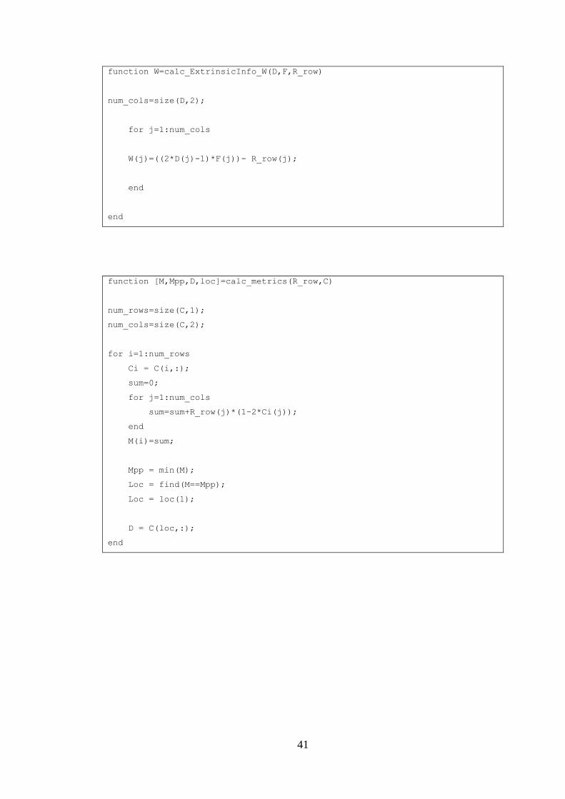
function W=calc_ExtrinsicInfo_W(D,F,R_row)

num_cols=size(D,2);

for j=1:num_cols

W(j)=((2*D(j)-1)*F(j))- R_row(j);

end

end

function [M,Mpp,D,loc]=calc_metrics(R_row,C)

num_rows=size(C,1);

num_cols=size(C,2);

for i=1:num_rows

Ci = C(i,:);

sum=0;

for j=1:num_cols

sum=sum+R_row(j)*(1-2*Ci(j));

end

M(i)=sum;

Mpp = min(M);

Loc = find(M==Mpp);

Loc = loc(1);

D = C(loc,:);

end

42

function [C,Si]=calc_SyndromesandCodewords(Z)

[parmat00,genmat,n,k] = hammgen(4);

num_col=size(Z,2);

C=Z;

Si = [];

for i=1:size(Z,1)

hi=Z(i,:);

syndrome = mod(hi * parmat00' ,2);

Si=[Si;syndrome];

col=syndrome';

ci=hi;

for k=1:num_col

parmat00_col=parmat00(:,k);

cond=numel(find(col==parmat00_col))==4;

if cond

ci(k)=~hi(k);

end

end

C(i,:)=ci;

end

function Tq=calc_test_patterns(R,p,P)

num_rows=2^p;

num_cols=size(R,2);

Tq=zeros(num_rows,num_cols);

perm_mat=double(dec2bin(0:2^p-1))-48;

for i=1:num_rows

Tq(i,P)=perm_mat(i,:);

end

43

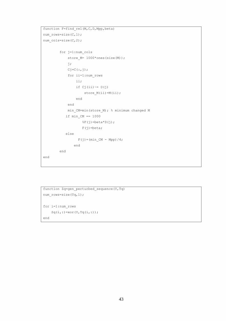
function F=find_rel(M,C,D,Mpp,beta)

num_rows=size(C,1);

num_cols=size(C,2);

for j=1:num_cols

store_M= 1000*ones(size(M));

j;

Cj=C(:,j);

for ii=1:num_rows

ii;

if Cj(ii)~= D(j)

store_M(ii)=M(ii);

end

end

min_CM=min(store_M); % minimum changed M

if min_CM == 1000

%F(j)=beta*D(j);

F(j)=beta;

else

F(j)=(min_CM - Mpp)/4;

end

end

end

function Zq=gen_perturbed_sequence(Y,Tq)

num_rows=size(Tq,1);

for i=1:num_rows

Zq(i,:)=xor(Y,Tq(i,:));

end

44

function [W,D]=half_iteration(R_row,beta)

[parmat00,genmat,n,k] = hammgen(4);

p=10;

% step1

R_abs= abs(R_row);

Y=(R_row>0);

% step2

[AA,index] = sort(R_abs);

Pos=index(1:p);

% step3

Tq=calc_test_patterns(R_row,p,Pos);

% step4

Zq=gen_perturbed_sequence(Y,Tq);

% step5

[C,Si]=calc_SyndromesandCodewords(Zq);

% step6

[M,Mpp,D,loc]=calc_metrics(R_row,C);

% step7

F=find_rel(M,C,D,Mpp,beta);

% step8

W=calc_ExtrinsicInfo_W(D,F,R_row);

45

% This is the main simulation program that uses the functions.

clear all

close all

clc

alpha=[0.0 0.2 0.3 0.5 0.7 0.9 1.0 1.0 1.0 1.0 ];

beta =[0.2 0.4 0.6 0.8 1.0 1.0 1.0 1.0 1.0 1.0 ];

%alpha=[0.0 0.1 0.2 0.25 0.3 0.35 0.4 0.45 0.5 0.55 0.6 0.65 0.7 0.9 1.0 1.0];

%beta =[0.2 0.3 0.4 0.45 0.5 0.55 0.6 0.65 0.7 0.75 0.8 0.9 1.0 1.0 1.0 1.0];

n=15; k=11; %Parameters of Linear block

code

info_word_length=k*k;

SNRdB=0:2:8; %SNR in dB

SNR=10.^(SNRdB./10); %SNR in linear scale

ber1=zeros(length(SNR),1); %Simulated BER fod SOFT Decoding

ber2=zeros(length(SNR),1);




%

for i=1:length(SNR)

SNR(1,i)

xj1=0;

xj2=0;

xj3=0;

xj4=0;

xj5=0;

repetition=1000;

for jj=1:repetition

% ==========================================================

% Start iterative decoding using Chase-Pyndiah algorithm

%

[R,msg,v]=received_signal(SNR(i));

% initializing W:

W=zeros(15,15);

46

m=1; % iteration-1

R1=R+W*alpha(2*(m-1)+1); % Input of row

decoding for 1st iteration

for k=1:15

R_row=R1(k,:);

[W1,D]=half_iteration(R_row,beta(2*(m-1)+1));

W(k,:)=W1;

end

R2=R+W*alpha(2*(m-1)+2); % Input of column decoding for

1st iteration

for k=1:15

R_col=R2(:,k);

[W1,D]=half_iteration(R_col',beta(2*(m-1)+2));

W(:,k)=W1;

end

out_it1 = W>0;

z1=length(find((msg ~= out_it1(5:15,5:15))));

xj1=xj1+z1 ;

m=2;

R1=R+W*alpha(2*(m-1)+1); % Input of row decoding for 2nd

iteration

for k=1:15

R_row=R1(k,:);


W(k,:)=W1;

end

R2=R+W*alpha(2*(m-1)+2); % Input of column decoding

for 2nd iteration

for k=1:15

R_col=R2(:,k);


W(:,k)=W1;

end

out_it2 = W > 0;

47


xj2=xj2+z2;

m=3;


iteration

for k=1:15

R_row=R1(k,:);


W(k,:)=W1;

end


for 2nd iteration

for k=1:15

R_col=R2(:,k);


W(:,k)=W1;

end

out_it3 = W > 0;


xj3=xj3+z3;

m=4;


iteration

for k=1:15

R_row=R1(k,:);


W(k,:)=W1;

end


for 2nd iteration

for k=1:15

R_col=R2(:,k);


W(:,k)=W1;

48

end

out_it4 = W > 0;


xj4=xj4+z4;

m=5;


iteration

for k=1:15

R_row=R1(k,:);


W(k,:)=W1;

end


for 2nd iteration

for k=1:15

R_col=R2(:,k);


W(:,k)=W1;

end

out_it5 = W > 0;


xj5=xj5+z5;

end

[xj1 xj2 xj3 xj4 xj5 ]

ber1(i,1)=xj1/(repetition*info_word_length);





end

[SNRdB' ber1 ber2 ber3 ber4 ber5]

figure

semilogy(SNRdB,ber1(:,1),'r-<','linewidth',2.0)

hold on;

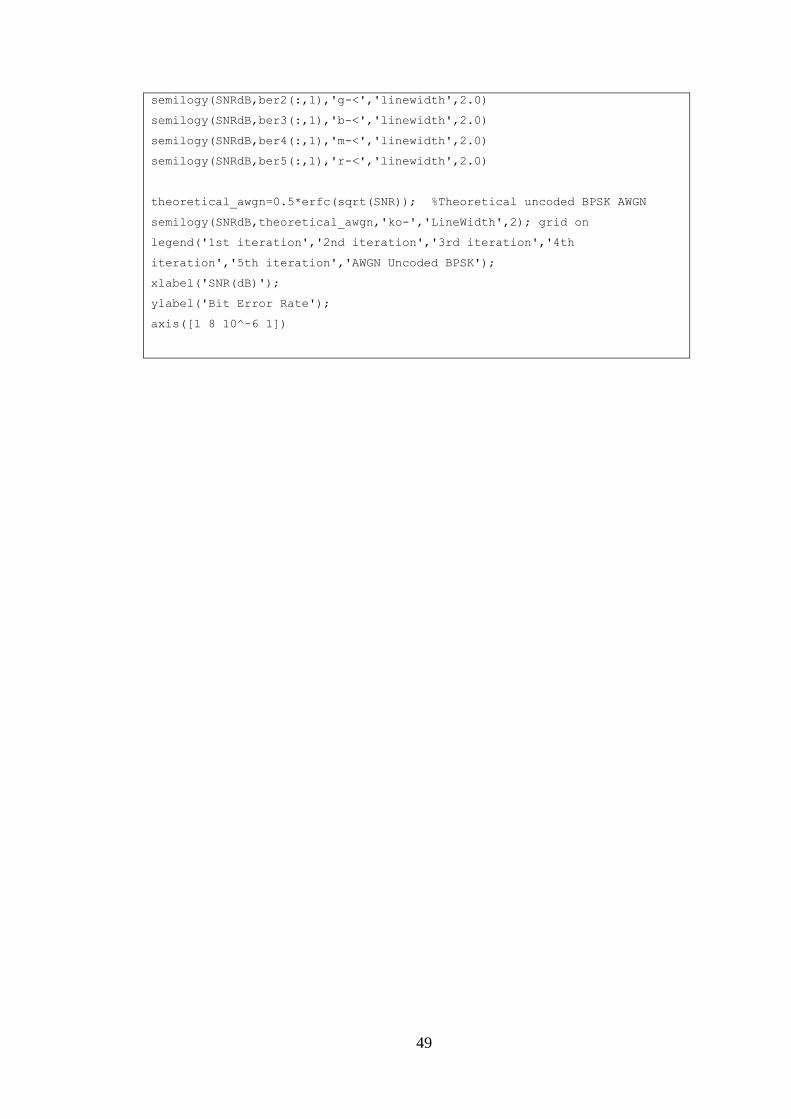
49

semilogy(SNRdB,ber2(:,1),'g-<','linewidth',2.0)

semilogy(SNRdB,ber3(:,1),'b-<','linewidth',2.0)

semilogy(SNRdB,ber4(:,1),'m-<','linewidth',2.0)

semilogy(SNRdB,ber5(:,1),'r-<','linewidth',2.0)

theoretical_awgn=0.5*erfc(sqrt(SNR)); %Theoretical uncoded BPSK AWGN

semilogy(SNRdB,theoretical_awgn,'ko-','LineWidth',2); grid on

legend('1st iteration','2nd iteration','3rd iteration','4th

iteration','5th iteration','AWGN Uncoded BPSK');

xlabel('SNR(dB)');

ylabel('Bit Error Rate');

axis([1 8 10^-6 1])

Iterative Decoding of Turbo Product Codes (TPCs)...

Documents

Transcript of Iterative Decoding of Turbo Product Codes (TPCs)...