PATTERN SYNTHESIS OF LINEAR AND CIRCULAR ARRAYS

by

Chuang-Jy Wu ,B.Eng.

A thesis submitted to the Faculty of Graduate Studies and Research in partial fulfillment of the requi~ments for the degree of Master of Engineering.

Department of Electrical Engineering, McGill University, Montreal. August, 1962

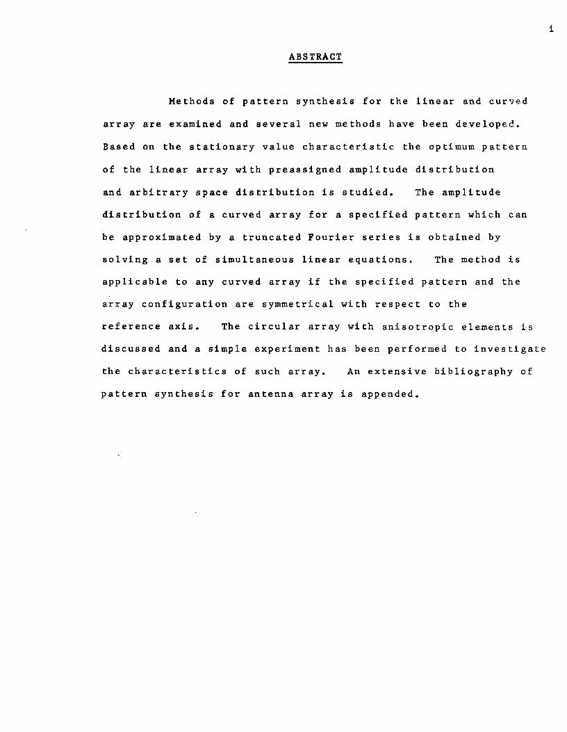
ABSTRACT

Methods of pattern synthesis for the linear and curved

array are examined and several new methods have been developed.

Based on the stationary value characteristic the optimum pattern

of the linear array with preassigned amplitude distribution

and arbitrary space distribution is studied. The amplitude

distribution of a curved array for a specified pattern which can

be approximated by a truncated Fourier series is obtained by

solving a set of simultaneous linear equations. The method is

applicable to any curved array if the specified pattern and the

array configuration are symmetrical with respect to the

reference axis. The circular array with anisotropie elements is

discussed and a simple experiment bas been performed to investigate

the characteristics of such array. An extensive bibliography of

pattern synthesis for antenna array is appended.

i

ACKNOWLEDGEMENTS

The author wishes to express his sincere gratitude to

Dr. T~J.F.Pavlasek for his patient guidance and constant

encouragement in the course of this research. He is also

greatly indebted to Mr. Y.F.tum for critical commenta and

invaluable help in preparing and reading the final draft of

the thesis. The author is grateful to the technical staff

at the Department of Electrical Engineering, McGill University

for their assistance, especially to Messrs. M.Zegel, P.Conroy,

E.Hauck, and J.Simms; to the staff of the Engineering

Library for their help in securing numerous inter-library

loans, to the staff of the Computing Centre for processing

the programmes, and to Mrs. J.R.Horner for doing such a fine

job in typing this thesis.

The author also gratefully acknowledges assistance from the

National Research Council, Ottawa, who provided the author with

two summer supplements and who financed the whole research

project (Grant No. A-515).

ii

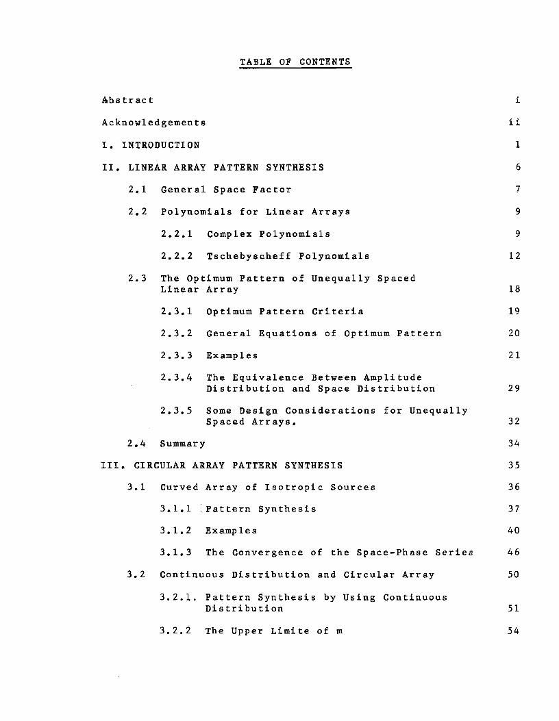
TABLE OF CONTENTS

Ahstract

Acknowledgements

I. INTRODUCTION

II. LINEAR ARRAY PATTERN SYNTHESIS

2.1 General Space Factor

2.2 Polynomiale for Linear Arrays

2.2.1 Complex Polynomiale

2.2.2 Tschebyscheff Polynomiale

2.3 The Optimum Pattern of Unequally Spaced Linear Array

i

ii

1

6

7

9

9

12

18

2.3.1 Optimum Pattern Criteria 19

2.3.2 General Equations of Optimum Pattern 20

2.3.3 Examp1es 21

2.3.4 The Equivalence Between Amplitude Distribution and Space Distribution 29

2.3.5 Some Design Considerations for Unequally Spaced Arrays. 32

2.4 Summary 34

III. CIRCULAR ARRAY PATTERN SYNTHESIS 35

3.1 Curved Array of Isotropie Sources 36

3.1.1 ~Pattern Synthesis 37

3.1.2 Examples 40

3.1.3 The Convergence of the Space-Phase Series 46

3.2 Continuous Distribution and Circular Array

3.2.1. Pattern Synthesis by Using Continuous Distribution

3.2.2 The Upper Limite of m

50

51

54

3.3 Circular Array of Anisbtro~ic Elements

IV. EXPERIMENTAL STUDY OF THE CIRCULAR ARRAY WITH ANISOTROPie 'ELEMENTS

4.1 Introduction

4.2 Experimental Arrangement

4.3 Measurements: The Circular Array with A~is6tro~ic· Elemeftts

V. CONCLUSION

BIBLIOGRAPHY

57

62

62

62

66

74

76

I. INTRODUCTION

The theory of pattern synthesis is concerned with

determining the relationsbip between the far-field pattern

of an array and the amplitudë and phase distribution of the

individual elements and their spacing. This is of utmost

importance in antenna design since if a single antenna is

unable to produce a desired pattern, it is usually feasible

to construct and use a system of antennas. This thesis is

restricted to the case of sources located on a straight

line or eurve.

In recent years, considerable attention bas been

given to the problem of synthesizing the patterns of linear

arrays and ring quasi-arrays. Most of the papers on pattern

synthesis in the early days of directional antenna design

dealt with broadcast antenna arrays witb equal magnitude

excitation of the elements, or with Yagi-type antennas

21 57 . (see Foster and Southworth • An extended bibl~ography of

antenna arrays before 1930 also appeared in Southworth 1 s

paper). Hansen and Woodyard 24 demonstrated that the gain of

a uniform endfire array could be increased by using an array

with larger values of phase differences between each element

than was customarily used. It was Schelkunoff 51 who first

introduced the polynomial formulation of the linear array problem.

By utilizing the correspondance between the pattern of an array

and the value of a complex polynomial on the unit circle, he

obtained an improved pattern by equally spacing the zeros of the

polynomial on an appropriate arc of the unit circle. The

optimum pattern was not achieved until Dolph 74 devised a

method using the characteristics of Tchebyscheff polynomials

to synthesize the broadside array with half-wavelength spacing

82 75 79 between elements. Later Riblet , DuHamel , Pritchard ,

Rhodes 81 and Sinclair and Cairns 84 extended Dloph's method

to the linear array with greater or less than half-wavelength

spacing, to the end-fire array and to the array with anisotropie

elements, 61 Recently, Unz proposed a method for pattern

synthesis of unequally spaced array by expanding the space-

phase terms of the space factor in an infinite series. Using

the stationary value method, the pattern of a linear array

with equal excitation and unequal spacing was obtained by

Pokrovskii45

• Most of the theoretical anaylses of linear arrays

rell on the assumption that the element patterns are identical,

in which case the pattern multiplication method can be applied.

Hines, Rumsey and Tice 28 attempted to modify the usual pattern

multiplication method which was useful only for obtaining the

first approximation for linear arrays.

Because of difficulties of analysis of the linear array

2

with .discrete elements. the theoretical study of continuous

distribution might be useful. It is a reasonable assumption

in the analysis that if the number of discrete elements is

large enough a continuous distribution can substitute for a

discrete array. Woodward and Lawson 67 investigated the

uniform amplitude line distribution with progressive phase

variation, and utilized the resulta to synthesize an arbitrary

pattern. By controlling the variation of the amplitude

distribution with known uniform phase or controlling variation

19 of phase with known amplitude distribution, Dunbar showed

that a specified beam shape may be obtained. 59 Taylor studied

line-source by means of function theory, and an ideal pattern

was established. 55 Shanks suggested a method of pattern

synthesis using variation of amplitude but with a specified

non-linear phase distribution. The technique might be useful

for large antenna design.

The prob1em of pattern synthesis of a circu1ar array

has been so1ved for some particu1ar cases. Expanding the

space-ph~se factor to a Fourier-Bessel series, Hansen and

24 114 96 101-106 Woodyard , Page , Harrington and Lepage and Knudsen

have analysed the circular array extensively. The difference

of array characteristics between uniform distributed elements

and the continuous distribution has been investigated in detail.

119 Taylor suggested a method whereby any prescribed pattern

representable by a truncated Fourier series can be obtained.

3

94 DuHamel derived the optimum pattern for antenna arrays on a

circular surface of small diameter. Using the fact that the

far-field pattern of the form cos n9 can be obtained by the

unifurm clrcular array with total progresslng phase distribution

2n1f 1 th i f Patton and Tillman llS a ong e c rcum erence~

introduced a method to syntheslze any specified pattern which

could be expanded in a Four~er series.

Although the subject of pattern synthesis has been

investigated for a long time, it is surprising that there are

not many methods available for synthesis of linear or curved

a:rrays. In fact very few problems can be solved by using

known methods. However, several known methods of pattern

synthesis for antenna array are described here, and their

applicability and the effectiYeness discuss~d.

There are two parts to the present work; the first

part (Chapter 2) deals with the optimum pattern of the

linear array, the second part (Chapters 3 and 4) is devoted

to the pattern synthesis of the curved array in general and

the circt\_lar array in pat·ticular.

Based on the existing theory of equally spaced linear

arrays, the relationship between the antenna array and the number

4

of nulls of the space factor will be discussed in Chapter 2,

and then the criteria of the optimum pattern for the linear

array will be stated. By using the stationary value character-

istic, the broadside optimum pattern can be obtained for the

unequally spaced linear array with known amplitude distribution.

From the calculated results of the optimum pattern, the

relationship between the space distribution and amplitude

distribution will be examined qualitatively.

In Chapter 3 a new method of pattern synthesis for the

curved array is derived by expressing the space-phase term

in a Fourier-Bessel series. The method is applicable to

any type of curved array so long as the geometrical

configuration is symmetric with respect to the pattern axis.

5

It is shown that the usual pattern synthesis method of the equally

spaced circular array by using continuous current distribution

is a special case of the new method.

Since a suitable analytical method of pattern synthesis

for the circular array with anisotropie elements cannot b~

established, an experimental method is performed, to investigate

the characteristics of such arrays. The experimental arrange­

ments and the results are shown in Chapter 4.

II. LINEAR ARRAY PATTERN SYNTHESIS

According to the beam shape, antenna beams can be

classified as pencil-beam, fanned-beam, shaped beam and

omnidirectional beam. A fanned-beam can usually be

obtained by simply reducing the corresponding dimension of

the aperture of a pencil-beam antenna, and an omnidirectional

beam may be produced by a half-wave antenna or an aperture

antenna. For the shaped-beam pattern, the method of synthesis

depends on the particular beam shape. However, these various

cases will not be discussed here and only the case of

pencil-beam antennas will be considered.

In order to simplify and generalize the methods of .

p•ttern synthesis, it is assumed that the pattern multiplication

method is valid and each elemental source bas an omnidirectional

pattern in the plane in which the pattern is synthesized.

Since the space phase difference between consecutive elements

for an equally spaced array is always the same, one can consider

the array factor as a (n-l)th order polynomial for an n-element

array and the variable of the polynomial varies along the

circumference of the unit circle in the complex plane. The

problem of pattern synthesis is then completely reduced to a

study of the properties of the complex polynomial. If the

spacing between each element is known, the amplitude

6

distribution of the arr~y, i.e. the coefficients of the

polynomial, can be simply determined by specifying the

position of the nulls in the specified pattern, i.e. the

ro~ts of the polynomial.

Since the space-phase differences of the successive

elements are different for an unequally spaced array, the space

factor becomes an irregular polynomial which cannot be

determined by specifying the roots of the polynomial. The

m-ethods of pattern synthesis for equally spaced arrays are

not applicable in this case. If the amplitude distribution

of the array is known, the space distribution may be determined

by using the stationary value characteristics of the specified

pattern.

In the following sections~ the methods of pattern

synthesis for equally spaced arrays will be discussed. .The

method of design for the optimum pattern of the antenna array

with specified amplitude distribution will be given and the

relationship between the space and amplitude distribution

will be studied.

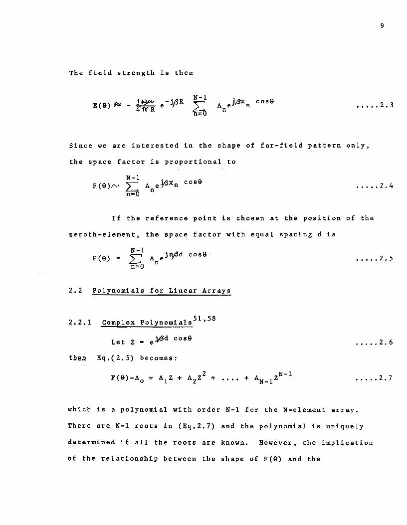
2.1 General Space Factor

The field strength (in RMKS system) at any point from

an array with isotropie elem~nts is:

7

N-1

E(9) = - t.ô ~ 4TI'r n

volts/me ter

where An is the current amplitude (magnitude and phase) of the

nth element in Amperes.

r is the distance between the nth element and the n

observing point, in meters.

is the permeability of free space, 4'fl'xl0- 7 henry/meter.

(3 = 2if/'A

À is wavelength in meters.

For a distant observing point, the phase factor becomes

r = (l -X ) • '1.:/R n n

8

= R -X cos 9 .....•••• 2.2 n

where R is the distance between the reference and observing

point.

/

G AH-1

~-----:-----il1,..;-------

Figure 2.1 Space Phase Difference Between any Element and Rèference Point

9

The field strength is then

N-1

~ J./5X. cos9 A e . n ..... 2.3

n

Since we are interested in the shape of far-field pattern only,

the space factor is proportional to

If the reference point is chosen at the position of the

zeroth-element, the space factor with equal spacing d is

2.2

2.2.1

F(9) = N-1 2:_ A ejty.3d n=O n

cos9 ·

Polynomiale for Linear Arrays

51 58 Complex Polynomiale '

Let Z = eldd cos9

tbea Eq.(2.5) becomes:

F(9)=A 0 + A1 z + A2 z2 + •••• + A ZN-1 N-1

••••• 2. 5

•..•• 2.6

. • • • • 2 • 7

which is a polynomial with order N-1 for the N-element array.

There are N-1 roots in (Eq.2.7) and the polynomial is uniquely

determined if all the roots are known. However, the implication

of the relationship between the shape of F(9) and the

corresponding roots have not yet been fully developed.

l' •.

Since Z is a complex variable with unit absolute

value, it is always on the circumference of the unit circle.

d=-"./4

(Cl)

Figure 2.2

d=3J\./4-

(C)

The Relations Between the Range of Z

and the Spacing d. (The values in the figure show the corresponding directions in space .. )

As 9 varies from 0° to 180°, Z moves from ej;.3d to e -j~d

in the clockwise direction. So the path of Z may be a portion

of the unit circle or several circuits of it depending on

whether the spacing d is smaller or larger ~han A/2,

(Figure 2.2).

If the roots of (Eq.2.7) are z1 , z2 ••••• ZN-l' then

10

0 •••• 2 .. 8

If the roots are on the circu•ference of the unit circ1e (i.e.

"Ad ·Ad unit •agnitude) within the region eJ,~ to e-Jr , then for d

less than or equal to ~/2, F(9) experiences N-1 zeros when 9

travels fro• 0° to 180°. There are at •ost N-1 lobes of the

space factor. If d is larger than ~/2, the point on the unit

circle corresponds to many values of the direction in physical

space. The nu•ber of nulls of the space factor may thus

exceed N-1, and correspondingly the number of lobes may also

be greater than N-1.

The value of F(9) is the product of the distances

from the corresponding value of Z to the roots. From this

property one can find that the relative value of F(9) is

largely influenced by the distance from Z to the nearest zero

of F(9) and the more re•ote zeros have less effect. It is

then obvious that the directivity can be increased by increasing

the number of zeros in the range, It should also be noted

that the spacing d of the endfire array, which has a main beam

in the direction 9=0 cannot equal or exceed À/2. If this

does happen, then as 9 varies from 0 to ~ , Z will pass through

the point (9•0) of maximum value more than once as shown in

Fisure 2.2 (b) and (c). The space factor then will have

several main beams and this is not desirable in most cases.

Since the main lobe of the broadside pattern is in the direction

9= rr/2, therefore the spacing d of such array cannot be equal to

or larger than À.

11

12

From the above discussion, the following conclusions

are arrived at:

(a) The spacing d must be less than À/2 for the endfire

array and, obviously, the maximum number of nulls will

be equal to N-1.

(b) The spacing d must be less than ~ for the broadside

array, and the maximum number of nulls in the space factor

can be equal to 2(N-l).

2.2.2 Tchebyscheff Polynomiale

For a symmetrically distributed linear array, the

resulting space factors are

(N-1)/2 F (9) = A + 2 ~ An cos 2n(,8d2 cos 9}

0 0 ~

for odd number of N, and

for even number of N. Let

and

()d cos9 =X 2

cosX =LI.·

the space factors become

F (~) = A + 2 0 0

(N-1)/2 2:. An cos 2n.X= P

0 ( tk

2)

n=l

••••• 2. 9 a

••••• 2. 9 b

••••• 2.10a

•••• 2.10b

•••• 2.lla

13

N/2 and Fe(9) • 2 2: An cos (2n-1)7'.S= U Pe(ll)

n•l •••• 2.llb

2 where P is a polynomial of U with degree (N-1)/2, and

0

2 P is a polynomial of U with degree N/2-1. e

The most desired features of pattern synthesis are

that a specified beam width and minor lobe level can be

obtained by adjusting the complex ratios of the currents in

the antenna elements. Although the complex polynomial

method can preassign the beam width accurately, the minor

lobe level is unknown until one calculates the extreme values.

Another problem of the usual space factor is that the minor

lobe level near the main beam is always the largest among

the minor lobes. If the first minor lobe level is decreased,

the level of other minor lobes is decreased simultaneously.

However, it is seldom necessary to decrease these side lobes

much below the first minor lobe, and in this sense the pattern

is not. bptimal.

Since the space factor of a symmetric array can be

expressed as a real polynomial, it is then possible to equate

the space factor F(9) to a known polynomial which has the

desired properties, and the amplitude distribution of the

antenna array can be obtained by using the method of

undet~rmined~ coefficients. Dolph74

used the properties of

Tchebyscheff polynomials for obtaining the optimum distribution

which bas minimum beam width if the minor lobe is assigned,

or a minimum magnitude of minor lobes if the beam width

is specified.

The Tchebyscheff polynomial is defined by

= cos (n cos-l V)

-1 = cosh (n cosh V)

which bas some important properties.

wh en IVI!::l.

wh en lVI~ 1.

Its maximum absolute

value in the range -1 :!f V~ 1 is smaller than any other real

polynomial of the same degree whose leading coefficient is

unity .. The extreme values of the Tchebyscheff polynomial in

the range -l!GV~l are equal, and the absolute value is

monotonically increasing outside this range. Clearly this

is the desired property for the space factor provided the range

of minor lobes can be made to coincide with the minimized range

of the polynomial. It will be found that not all

configurations can satisfy this condition. According to the

direction of the main lobe and the spacing four classifications

the can be recognized, but onlyAtwo broadside array cases will be

discussed and the two endfire array cases would be considered

in a similar fashion.

14

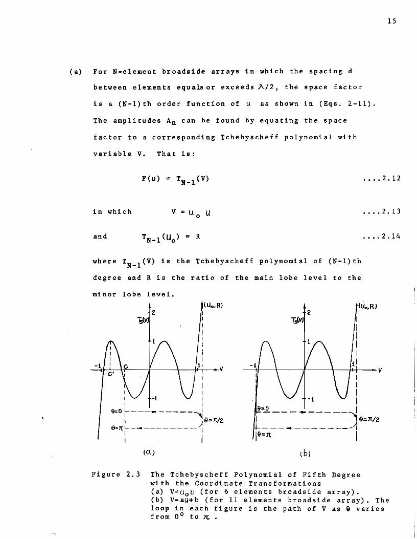
15

(a) For N-element broadside arrays in which the spacing d

between elements equalsor exceeds À/2, the space factor

is a (N-l)th order function of u as shown in (Eqs. 2-11).

The amplitudes An can be found by equating the space

factor to a corresponding Tchebyscheff polynomial with

variable V. That is:

F(U) '"' TN-l (V)

in wh i ch V = U U 0

where TN_1

(V) is the Tchebyscheff polynomial of (N-l)th

degree and R is the ratio of the main lobe level to the

miner lobe level.

-1 C'

1 1

z Ts(V)

1 1

(U •• R)

1

1 1

-1 1

•••• 2. 12

•••. 2. 13

•••. 2. 14

9=0 ~---------~ 1 . )9=7t/2

9:JLL----------- 1

9=0 ----------~ L- ___ ---------19::1t/2

: 1 jQ=n 1

lO.) l bJ

Figure 2.3 The Tchebyscheff Polynomial of Fifth Degree with the Coordinate Transformations (a) V=u 0 U (for 6 elements broadside array). (b) V=aU+b (for 11 elements broadside array). The loop in each figure is the path of V as 9 varies from 0° to Jt. •

16

The transformation (Eq.2.13) constitutes a scale amplification

which makes the range of U (=cos(~~ cos9)) equivalent to

the range C ~v ~U0 , where C =U0

cos(~d/2) and C=O when

d = Â/2. (Figure 2.3(a)). The minimized range of the

Tchebyscheff polynomial is thus covered by using

transformation (Eq.2.13). The number of nulls of the

space factor, in this case, is equal to,or larger than,

N-1 depending on whether d = .:J\../ 2 or d >./\./ 2.

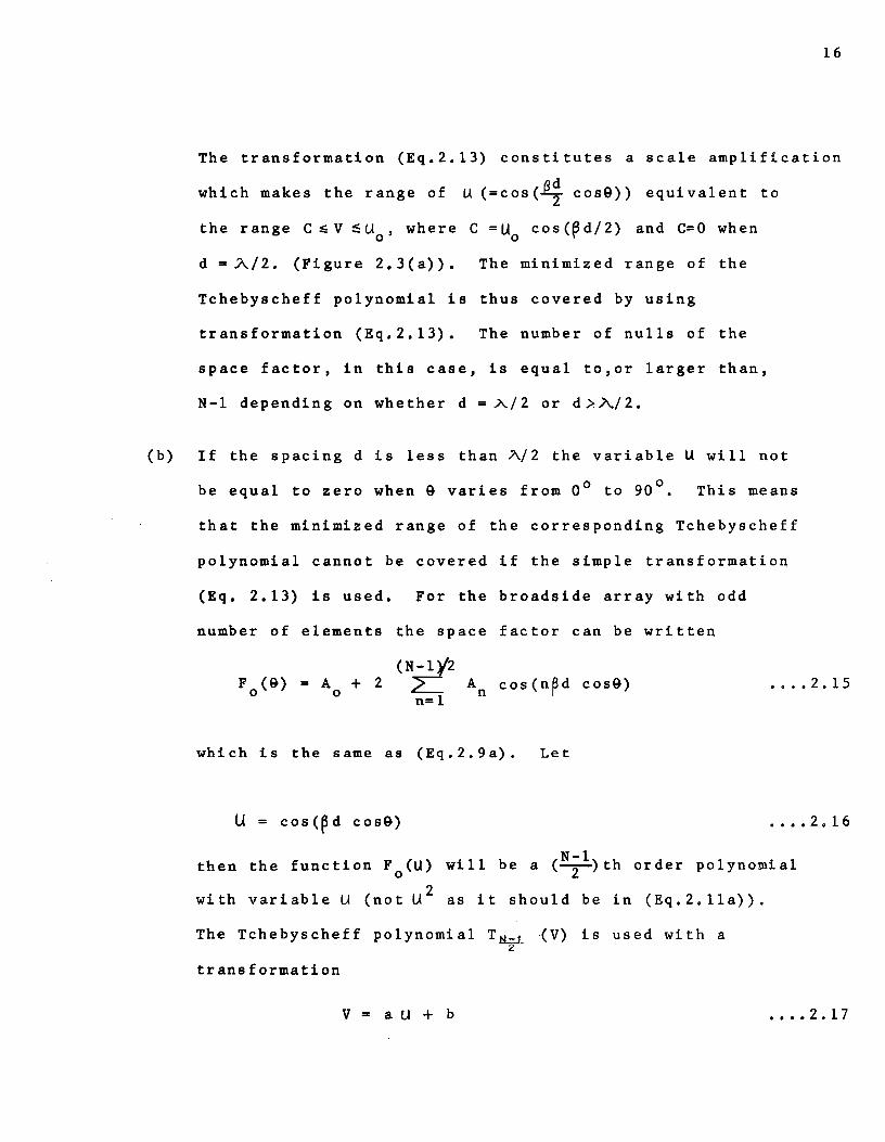
(b) If the spacing d is less than Â/2 the variable U will not

be equal to zero when 9 varies from 0° to 90°. This means

that the minimized range of the corresponding Tchebyscheff

polynomial cannot be covered if the simple transformation

(Eq. 2.13) is used. For the broadside array with odd

number of elements the space factor can be written

F (9) = 0

A 0

(N-1}'2 + 2 ~ A cos(npd cos9)

n=l n

which is the same as (Eq.2.9a). Let

•.•• 2. 15

U = cos(~d cos9) •••• 2.16

th en N-1 the function F

0(U) will be a (---2-)th arder polynomial

with 2 variable U (not U as it should be in (Eq. 2.lla)).

The Tchebyscheff polynomial T~_ (V) is used with a 2

transformation

V=aU+b •••• 2. 17

17

where a and b are constants which are determined by the

conditions

-1 = a cos ~ d + b ••• 2.18a

Ua= a + b .•. 2.18b

and ••• 2.18c

The values An can then be solved by the following equation:

T·~t [ a cos ( ~ d cos 9) + b J = F 0

[cos (Pd cos 9) J (Eq.2.17) is a linear transformation which enables the range

of U =cos (~d cos9) to be equivalent to the range -1!::: U !:": U0

of the Tchebyscheff polynomial T~ (U) as 9 varies from 2.

0° to 90° (as shown in Figure 2.3(b)). There are thus

exactly N-1 nulls in the space factor.

All the transformations~ which are used in the different

array configurations ensure that the main beam will point in the

desired direction and the number of nulls of the space factor

is equal to or greater than N-1, where N is the number of

elements. If the number of nulls is less than (N-1) the

space pattern is not optimum even if the minor lobes are of

equal magnitude. This is the reason why transformation (b) is

introduced.

It should be noted that in the Tchebyscheff distribution

the amplitude in the inner elements is usually larger than the

amplitude of the outer elements except when R (ratio of main

lobe to minor lobe level) is small. The amplitude ratio of the

center elements to the edge elements reaches maximum when

R ~oo which is the so-called binomial distribution. The

amplitude ratio will be equal to zero when R = 1, in this case~

the amplitude of all the elements are equal to zero except

the edge elements. Thus both the binomial and edge distributions

are the limiting cases of the Tchebyscheff distribution, and the

a•plitude ratio decreases when R decreases.

2.3 The Optimum Pattern of Unequally Spaced Linear Array

The space patternF(cos9) of an antenna array is a

function of the amplitude distribution and spacing. In the

investigations carried out so far, the spacing is usually

specified and one then adjusts the amplitude of the elements to

obtain a desirable pattern. The spacing in most cases is

equal at some arbitrary value. However, if the amplitude and

spacing ean both be adjusted, the optimum utilization of these

two parameters might be achieved. In the following section, a

general method of optimua pattern synthesis with arbitrary

spacing and non-uniform excitation is developed. The

relationship between amplitude and space distribution is

qualitatively studied in terms of an example.

18

2.3.1 Optimum Pattern Criteria

In the section 2.2~2 it was shown that for an equally

spaced linear array with a fixed number of elements and

specified spacing, the optimum amplitude distribution is

usually defined in such a way that, if the minor lobe is

assigned, the beam widtp is a minimum, or conversely, if the

beam width is spe~ified, the minor lobe level is minimized

and thus the space pattern bas equal magnitude minor lobes

and (N-1) nulls.

~t was also shown qualitatively that the larger the

nvmber of nulls that the space pattern bas, the more directive

it is. The maximum number of nulls of an N-element equally

spaced array is usually equal to N-1, and may exceed N-1 in

some cases, but not over 2(N-l). Thus the most important

19

factors for the optimum pattern are the number of nulls which

effects the directivity of the space pattern, and the characteristic

of equal magnitude minor lobes. Bence we shall define the

optimum pattern as one which possesses the following character­

istics.

(a) The space pattern bas at least N-1 nulls for N-element array.

(b) The space pattern bas one main lobe and equal level minor

lobes.

The problem of optimum pattern synthesis then centres on the

20

aua\ysis of the function properties instead of dealing with the

polynomial characteristics as is done in the equally spaced

ar ray;

2.3.2 General Equations of Optimum Pattern

Define:

••• 2. 19

where 9 is the direction of the main beam 0

9i is the direction of the ith minor lobe, and

i =~1, 2 ••••• 2(N-l).

Let the ratio of the main lobe level to the minor lobe level

be R. Then the conditions for the optimum pattern can be

described by the following equations:

F ( C( 0

) = R

F( <Xi) = (..:l)i 1 • 1, 2, ••••• 2(N-l)

Ft (cl.) 1 • 0( =<Xi aF j d =0( == o aa 1

i,.. O,l, ••• (2N-3)

••• 2.20a

••• 2.20b

••• 2.20c

Since there are at most 2(N-1) nulls in the space pattern,

the number of equations in the form of (Eqs. 2.20b and 2.20c)

may be 2(N-l). The maximum number of unknowns may be 4N-3 with

2N-3 unknown directions ~1 • In order to obtain the non-trivial

solutions, a set of independent and consistent equations should

21

be chosen from (Eqs. 2.20).

In order to simplify the discussion, a broadside pattern

is used. Since the broadside pattern is symmetrical with respect

to the normal of the array, there are at most N-1 nulls at each

side of the main beam. Equations (2.20) consequently reduce

to the following form:

F(O) = R ••• 2.21a

F(CXi) = (-l)i i = 1' 2, ••• N-1 ••• 2.21b

F' ( O:i) = 0 i = 1,2, •••• N-2 .•. 2.2lc

If the amplitude distribution is specified, there are N/2

or (N-1)/2 unknowns in the spacing between elements depending

on whether N is even or odd. In order to utilize the maximum

number of minor lobes, the following set of conditions is

suggested:

A•F(O) = R

A"F(0:1 ) = -1

A•F'(a.) = 0 :. 1

A•F(.l) = (-l)N/2 (-I)(N-1)/2

where A is a normalizing constant.

2.3.3 Examples

for N is even for N is odd

The following simple examples are given in order to

••• 2. 2 2

22

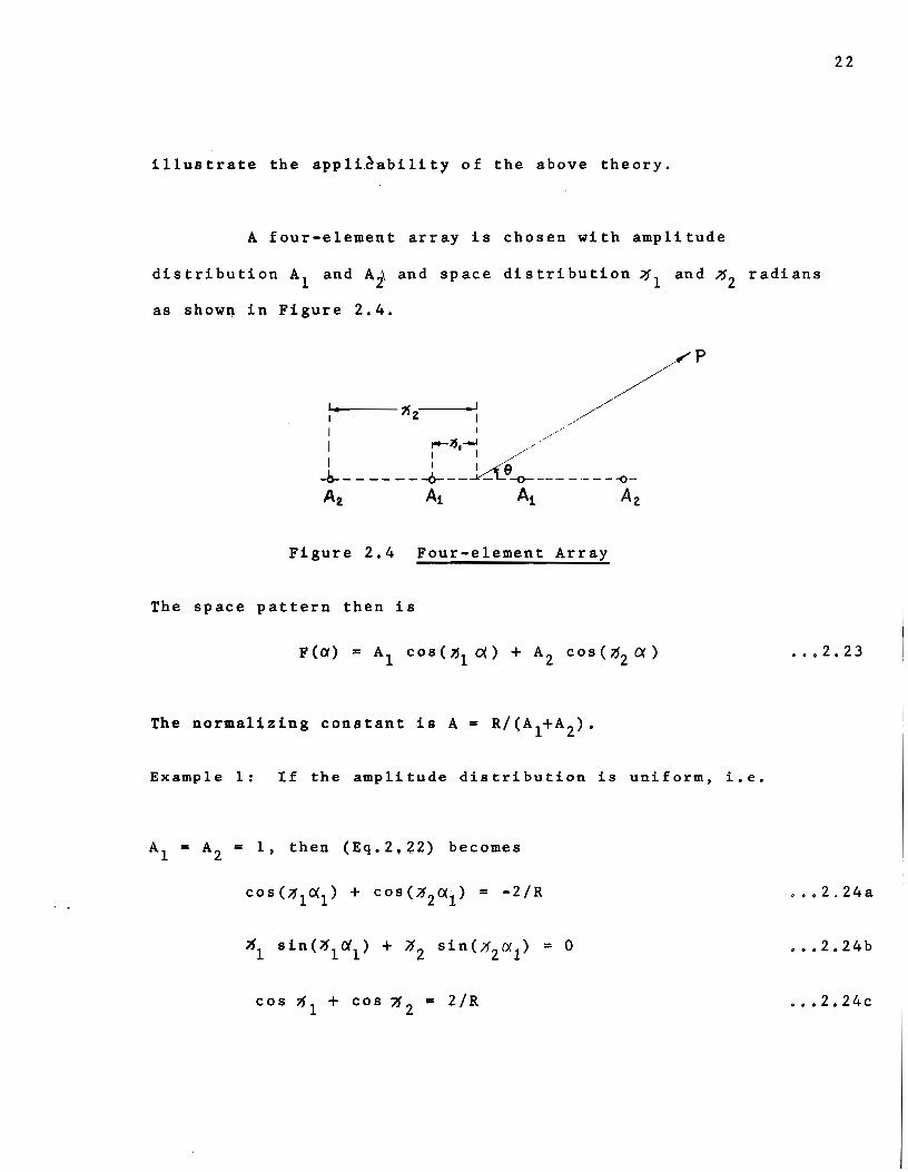
illustrate the appliAability of the above theory.

A four•element array is chosen with amplitude

distribution A1

and A~ and space distribution ~l and ~2 radians

as show~ in Figure 2.4.

-----~z·--__.}

Figure 2.4 Four~element Array

The space pattern then is

••• 2. 2 3

The normalizing constant is A= R/(A 1+A 2).

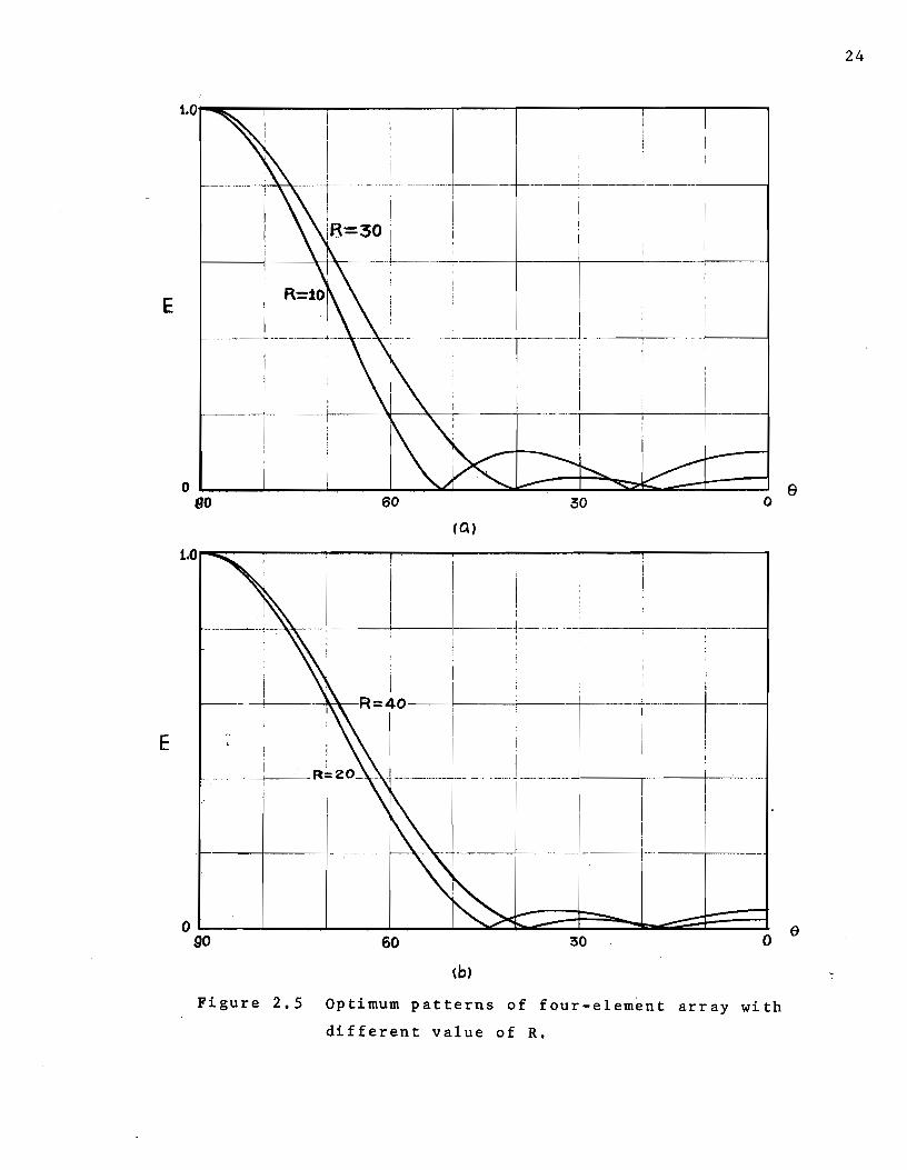
Example 1: If the amplitude distribution is uniform, i.e.

A1 = A2 = 1, then (Eq.2,22) becomes

••• 2.24a

.•. 2.24b

cos i'fl +cos 7! 2 "" 2/R ••• 2.24c

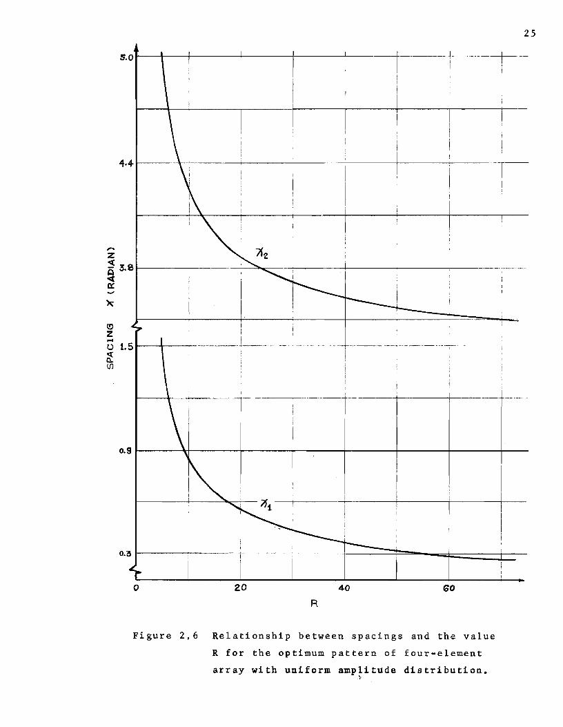
The resultant patterns are shown in Figure 2.5, with R=10,20,

30 and 40 and the relationship between R and ~l and 4 2 are

shown in Figure 2.6.

It is worthwhile to note that the spacings ;1 1 and ?J 2

decrease as R increases (Figure 2.6). If R approaches

infinity, it means that there are no minor lobes in the space

pattern. Then the spacing ~l approaches zero and the spacing ~2 approaches n, and the amplitude of the centre element becomes

2. (The centre elements are squeezed together). This is the

binomial distribution with half wavelength spacing. If R is

equal to unity, then ~l = ~2 = 2~ , and the array degenerates

to a two-element one with one wavelength spacing (edge

distribution). These two limiting cases are the same as the

Tchebyscheff distribution.

The total length of the array is generally shorter

than the equally spaced array with half wavelength spacing

except when R is apprionmately smaller than 5 as shown in

Figure 2.6, and the beam width is larger than the array with

Tchebyscheff distribution. This result agrees with the general

theory of antennas, that is, for equal number of elements, the

smaller the aperture, the larger the beam width. However, the

uniform amplitude distribution can be easily obtained in

practice, and the beam width can always be reduced by using

more elements in the array. Thus the optimum pattern of

unequally spaced array may be useful in practical application.

23

E

E

(Q)

t.o..--::----.---,----,--......---------...,.-----ï

1

1

~-------;-----~~-· ---·

l 1

---1--.----tn:--R=~O-·_j_·---i----+-----~-r--·--

1 1 ! 1

·l·--·-·-··--·-· ··-·· . -···· --·······-----l----,-------t--------1

Figure 2.5 Optimum patterns of four-element array with

different value of R.

24

a

25

~0~~+-~~~~--~--------+--------+--------r-------~

4·4-1----

,... z <( ~ 3.8

0:

(!J

z ..... t) 1. 5 ._-4----~ (j)

--+------·---~--1' __ ---~, ---------t----+----+----· --·-·---- . 1 1 1

1 ' 1 :

0.9 ~------~------~--------+--------+--------r-------~------_, __ ___

--~----r----+-----~---~ : 1

0 20 40 GO

R

Figure 2,6 Relationship between spacings and the value

R for the optimum pattern of four-element

array with uniform amplitude distribution • . }

1 1

26

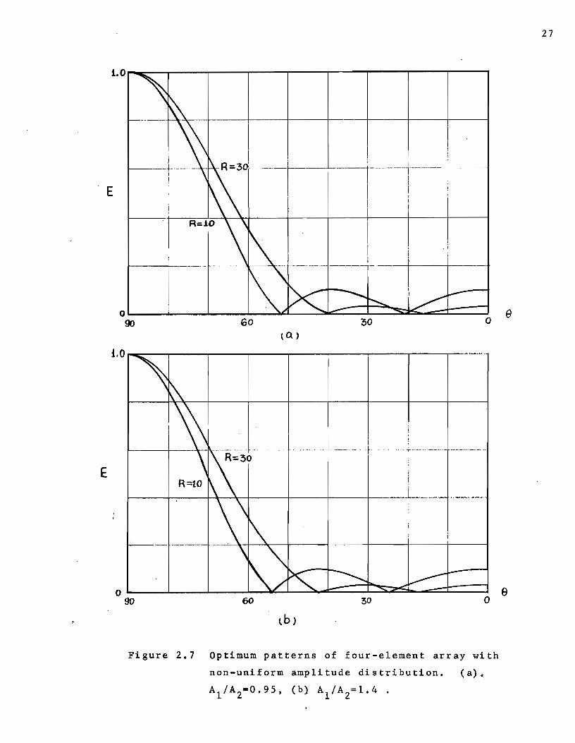
Example 2: If the amplitude distribution is non-uniform,

and the amplitude ratio is A1 /A2 , then (Eq.2.22) becomes:

.•. 2.25a

••• 2.25b

•.• 2.25c

The resulting patterns are shown in Figure 2.7 with R=lO and 30

The spacings .711 and 712 when A1

/A2

::: 0.95 is shorter

th an the spacings at uniform distribution and the spacings -"'1

and 7J2 when A1 /A 2 = 1.4 are larger th an the spacings at

uniform distribution as shown in Table 2.1.

TABLE 2.1 Variations of Spacings ,.1

and ?1 2

with Different

Values of A1 /A 2 and R.

~1 (radian) Jf2

(radian)

R==lO 0.7338 4.1766

R•30 0.2074 3.6680

R=lO 0.8510 4.2353

R=30 0.4310 3.7116

R=lO 1.'4246 4. 7 484

R=30 1.0551 4.0558

1.0~~~----~--~----~----,---~----~--~----~

E

E

1

1 1

R 'Zo.' 1

~------<--+--·-«--+++ :.., ----r·----1

1-----!----~-+----t---t-----L-·-r---. i

Figur~ 2.7 Optimum patt~rns of four-element array with

non-uniform amplitude distribution. (a)«

A1/A 2=0.95, (b) A1

/A2=1.4 .

27

e

e

EXAMPLE 3: If the amplitude distribution A1 and A2

and space

distribution 7}1

and 7{2

are variables, then (Eq.2.21) becomes:

28

••• 2.26

A1 cos ~l + A2 cos ~2 • 1

It is found that the array behaves as an equally spaced

one with Tchebyscheff amplitude distribution. The spacing which can

be easily determined from· transformation (a) Section 2.2.2, depends

..i.. on the minor lobe level R and is larger than J\../2. If the

spacing is d, then for four-element array

u cos 0

~d 2= cos 2n:

3

where U is the same as the definition in Section 2.2.2, 0

transformation (a). 0 This means that, when c< is equal to l(or 9•0 ) •

J F(~)f is equal to 1 which is the extreme value of the Tchebyscheff

v polynomial a=t point C'. as shawn in Figure 2.3(a).

c.orre:spond inj +o +he

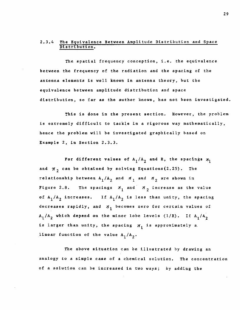
2.3.4 The Eq~ivalence Between Amplit~de Distrib~tion and Space Distribution,

The spatial frequency conception, i.e. the equivalence

between the frequency of the radiation and the spacing of the

antenna elements is well known in antenna theory, but the

equivalence between amplitude distribution and space

29

distribution, so far as the author knows, bas not been investigated.

This is done in the present section. However, the problem

is e~tremely difficult to tackle in a rigorous way mathematically,

bence the problem will be investigated graphically based on

Example 2, in Section 2.3.3.

For different values of A1 /A 2 and R, the spac1ngs ~l

and ?f 2 can be obtained by solving Equations (2. 25). The

re 1 a ti ons hi p be tween A1 1 A

2 and })'

1 and 7$

2 are shown in

Figure 2.8. The spacings JJ1

and· 7$2

increase as the value

of A1 /A 2 increases. If A1 /A 2 is less than unity, the spacing

decreases rapidly, and 7$ 1 becomes zero for certain values of

A1

/A2 which depend on the minor lobe levels (1/R).

is larger than unity, the spacing /fl is approximately a,

linear function of the value A1

/A2

•

The above situation can be illustrated by drawing an

analogy to a simple cas~ of a chemical sol~tion. The concentration

of a solution can be increased in two ways; by adding the

A Az

1.4•~------1----·-l------- J i 1

1.2. 1-------·

1.1

o.g

0.8

Figure 2.8 Relationship between A1 /A 2 and spacings x1

and x 2 for the

optimum pattern of four-element array,

4.7 1 7f SPACING

(RADAIN)

w 0

substance which is dissolved in the solution or decreasing the

amount of solvent. The amplitude of each element is analogous

to the substance in the solution and the spacing to the solvent.

For an optimum pattern (or Tchebyscheff distribution in equally

spaced array), it bas been shown in Section 2.2.2 that the

amplitude ratio of the inner elements to the outer elements

increases if R increases and the value is larger than 1 in

most cases. In other words, if the sum of the amplitudes is

constant, the concentration of the amplitude in the inner

elements will be increased by increasing the value of R. If the

amplitude distribution is fixed, as in a uniform distribution,

the only possible way to increase the amplitude concentration

for the inner elements is by reducing the spacing of the inner

elements. This is the reason why, for a four-element array with

uniform distribution, the spacing 2~1 between the two inner

elements is smaller than the spacing ( »2 - ~1 ) between the

inner element and the outer element, and ~ 1 is decreased

as R is increased. If the value of A1 /A2 is less than unity,

the spacing ~l must be smaller than the corresponding spacing

in the uniform amplitude distribution in order to compensate

for reduced amplitude. It is obvious that the spacing ~l will

be equal to zero at a certain value of A1 /A2 • If the value

A1 /A2 is below this critical value, no optimum pattern can

' be obtained by adjusting the spacing. There is also a

similar limitation as ~l is increased. Since the spacing ~l

is limited by two factors: i.e.

31

(a) the spacing 16 2 and

(b) the fundamental characteristics of the single main beam

linear array, namely, the spacing between successive

elements must be less than one wavelength.

Thus the value of A1

/A 2 cannot be increased indefinitely, and

..L the maximum value of A

1/A

2 depends on the minor lobe level R.

Although the analysis is based on the example of a four-element

array, it is believed that the concept is valid for the linear

array with elements more than four.

2.3.5 Sorne Design Considerations for Unequally Spaced Arrays

The design of an antenna system is a manifold problem

which involves the radiation resistance, mutual coupling,

the characteristic of the transmitter, efficiency, accuracy,

etc., and a complete discussion is beyond this thesis.

Ignoring the effect of radiation impedance which is very

important in the practical applications, a qualitative dis-

cussion of pattern formation will be given.

If the spacing is determined according to a uniform

amplitude distribution, the main beam is hardly affected

if the amplitudes or the spacings have ten percent deviation

from the design value, and in some ca~es the half-power beam

width might be narrower than the design value at the expense ,..

of a largely increased minor lobe level; but the minor lobe

32

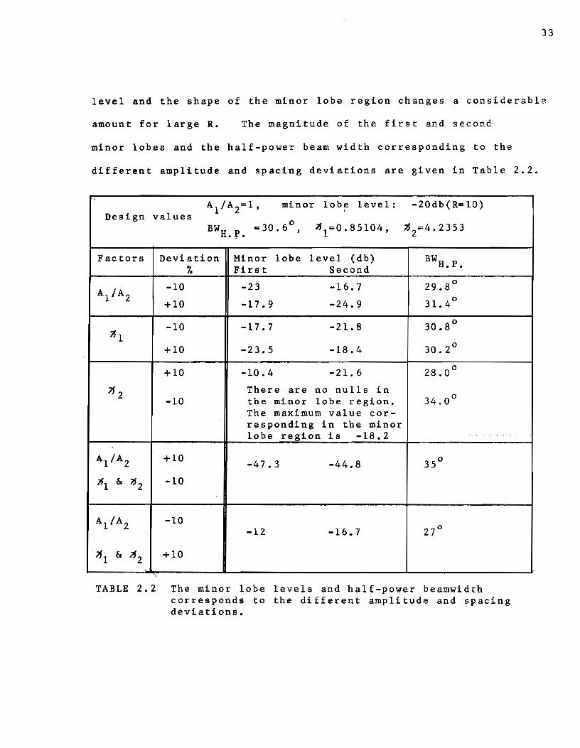
33

level and the shape of the minor lobe region changes a considerable

amount for large R. The magnitude of the first and second

minor lobes and the half-power beam width corresponding to the

different amplitude and spacing deviations are given in Table 2.2.

A1 /A 2=1, min or lobe level: - 2 0 db ( R= 1 0 ) ' Design values

0 J$1=0.85104, ~2=4.2353 BWH.f. =30.6 '

Factors Deviation Mi nor lobe level (db) BWH.P. % First Second

Al/A2 .. 10 -23 -16.7 29.8°

+10 -17.9 -24.9 31.4°

7fl -10 -17.7 -21.8 30.8°

+10 -23.5 -18.4 30.2°

+10 -10.4 -21.6 28.0°

712 The re are no nulls in -10 the mi nor lobe region. 34.0°

The maximum value cor-responding in the minor lobe region is -18.2 ..

Al/A2 +10 -47.3 -44.8 35°

}.fl & })2 -10

Al/A2 -10 -12 -16.7 27°

/11 & lf2 +10

'\

TABLE 2.2 The minor lobe levels and half-power beamwidth corresponds to the different amplitude and spacing deviations.

It is interesting to note that if A1 /A 2 increases ten

percent and both nl and ~2 decrease ten percent, the minor

lobe level is far below the design value, conversely, if A1/A 2

decreases ten percent and both ~l and ~ 2 increases ten

percent, the minor lobe level increases.

2.4 Summary

A general definition of an optimum pattern has been

introduced based on the characteristics of complex polynomials

and the properties of Tchebyscheff polynomial amplitude

distribution. It has been shawn that the optimum pattern of

a linear array with known amplitude distribution can be

obtained by adjusting the inter-element spacing. If the

relationship between the space distribution and the amplitude

distribution can be further developed, it may be possible in the

future that the unequally spaced array can be considered as an

equally spaced one with non-uniform amplitude distribution.

34

III. CIRCULAR ARRAY PATTERN SYNTHESIS

An array of rotational symmetry with respect to an axis

perpendicular to the horizontal plane is useful in applications

requiring an omnidirectional field or a rotating beam. The

circular geometry has the desired characteristic and a

configuration of a number of identical antennas uniformly

distributed along the circumference of a circle bas been used

in radio direction finding, radar and other applications.

Three variations are used in practice; the vertical dipoles

equally spaced on a circle either with or without a concentric

reflecting cylinder and the slot antennas on a cylinder.

Since the radiation pattern of the array depends not only

on the number of elements, spacing and amplitude distribution

but also on the orientation of the antennas, there are two

problems in the analysis of the curved array, or the circular

array. First of all the antennas of the curved array are

oriented in different directions, and the element pattern and the

space factor are not separable. The usual pattern multiplication

method, which simplifies the analysis in the linear array is

no longer useful. Secondly, the curved array is a two

dimensional problem and the exponential part of the space-

phase term is not a linear function of position. The polynomial

character~stic which is used in the linear array, is not

applicable in this case. As a first approach, a series

35

expression of the element factor and the space phase term is

attempted for the curved array pattern synthesis. This method

is of course limited by the convergence of the series. In

practice, the physical conditions may not fully satisfy the

mathematical conditions which are necessary for the existing

analytical methods. On the other hand, the numerical or the

experimental method for pattern synthesis seems to be promising.

A new method of pattern synthesis for the curved array

will be given in this chapter. The method is valid for any

type of two-dimensional array which is symmetric with respect

to the pattern axis provided that the number of elements is

large enough. The convergence of the Fourier-Bessel series

will be investigated. The circular array with an~stropic

elements will be discussed based on the theoretical analysis of

the circular array with isotropie elements.

3.1 Curved Array of Isotropie Sources

The method of pattern synthesis for the curved array

of isotropie sources to be developed in this section is based

~n a series expansion of the space-phase term. It is applicable

to almost any curved array which is symmetric with respect to the

major axis.

36

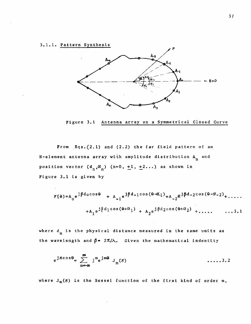
3.1.1. Pattern Synthesis

Figure 3.1 Antenna array on a Symmetrical Cl~sed Curve

From Eqs.(2.1) and (2.2) the far field pattern of an

N-element antenna array with amplitude distribution A and n

position vector (dn,an) (n=O, +1, +2 ••• ) as shown in

Figure 3.1 is given by

37

••• 3. 1

where d is the physical distance measured in the same units as n

the wavelength and P= 2X/~. Given the mathematical indentity

jJScos~ e = .m jm~ J (/J)

J e m ••••• 3. 2 m=-œ

where Jm(~) is the Bessel function of the first kind of order m,

and substituting (Eq.3.2) into the general array factor (Eq.3.1),

we obtain:

Jm(~d-1) +. • • •

+Al ~jmejm(9+1Xl) A L._. 3m(rdl) + ...... m•-œ

• • • • • 3 .. 3

If the antenna array is sy~metrical with respect to the

axis 9=0, i.e. A-n= An, and 0( -n = (X n (bence d = d ) then -n n

(Eq. 3. 3) becomes

where)..(N = 1 if the total number of elements N is even

= 0 if the total number of elements N is odd.

By using the identity

m J-m(~) = (-1) Jm(~)

Equation 3.4 can be written as

••••• 3. 4

••••• 3 .. 5

38

where E = 1 for m = 0

= 2 for m ~ 0

F(&) above is the pattern produced by a physical antenna

array (Figure 3.1). However. the amplitude distribution

A and bence F(&) are yet undefined. In pattern synthesis, the n

aim is to find an amplitude distribution that produces a

desired pattern for a given antenna system.

If the desired pattern S(&) is symmetric with respect to

the axis &=0, and also expressible as a Fourier series, then

00

S (&) = ~Sm cosm& ••••• 3. 6 m=o

where S are the Fourier coefficients and are determined by m

the pattern specification.

Equating 1

Eqs .. (3.5)and(3.6) we have

S /J.me = A J (Ad ) + 2A a J (Rd ) 2A a J (Ad ) m 0 m r 0 1cosm 1 m r 1 + zcosm z" m r 2

••••• 3. 7

where m = 0, 1, 2 ••• Since d and d are known, there are n n

(N+2)/2 (when N is eve~) or (N+l)/2 (when N is odd) number

of unknowns of the amplitude A , in other words, the number n

of equations is dependent on the number of elements used.

39

40

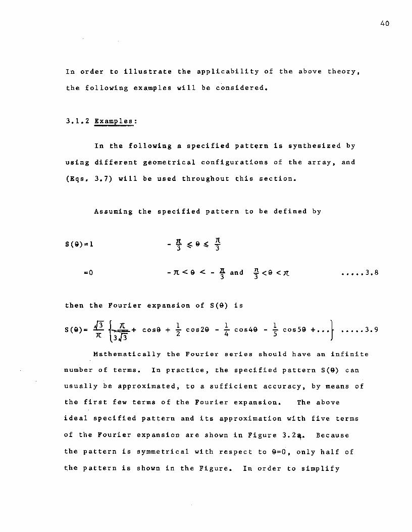
In order to illustrate the applicability of the above theory,

the following examples will be considered.

3.1.2 Examples:

In the following a specified pattern is synthesized by

using different geometrical configurations of the array, and

(Eqs. 3.7) will be used throughout this section.

Assuming the specified pattern to be defined by

8 (9)= 1

=0 - 7t < 9 < - i' and ~ < 9 < 1C ••••• 3. 8

then the Fourier expansion of 8(9) is

8{9)= di j~+ cos9 + ~ cos29-! cos49-; cos59 + ••• } ••••• 3.9 11: l3J3

Mathematically the Fourier series should have an infinite

number of terms. In practice, the specified pattern S(9) can

usually be approximated, to a sufficient accuracy, by means of

the first few terms of the Fourier expansion. The above

ideal specified pattern and its approximation with five terms

of the Fourier expansion are shown in Figure 3.2~. Because

the pattern is symmetrical with respect to 9=0, only half of

the pattern is shown in the Figure. In order to simplify

the calculations, some simple array configurations are

illustrated in the following.

CONFIGURATION I: Ten-element array equally distributed on

the circumference of a circle with radius d=~/2.

If the curve is a circle, then d0

= d 1 = d 2 ••• :d,

and (Eq. 3.7) becomes

41

••••• 3. 10

For the 10-element array, the number of equations will be

equal to six. Since it is equally distributed, then

a = n1C/ 5 n

The relative currents are

A0

= -2.576 - j 0.3712, A1= -0.535 - j 2.217,

A2= -0.9194 + j 0.6173, A3= -0.9194 - j 0.6173,

; A 4 = -o. s 3 s + j 2. 211 , A5= -2.576 +f o.3712.

The r esu 1 tàn t normal i z ed pat te rn i s .shown in Fi gu re

3.2b, and it is fairly near to the approximated Fourier

expansion. Although the minor lobe level is slightly higher

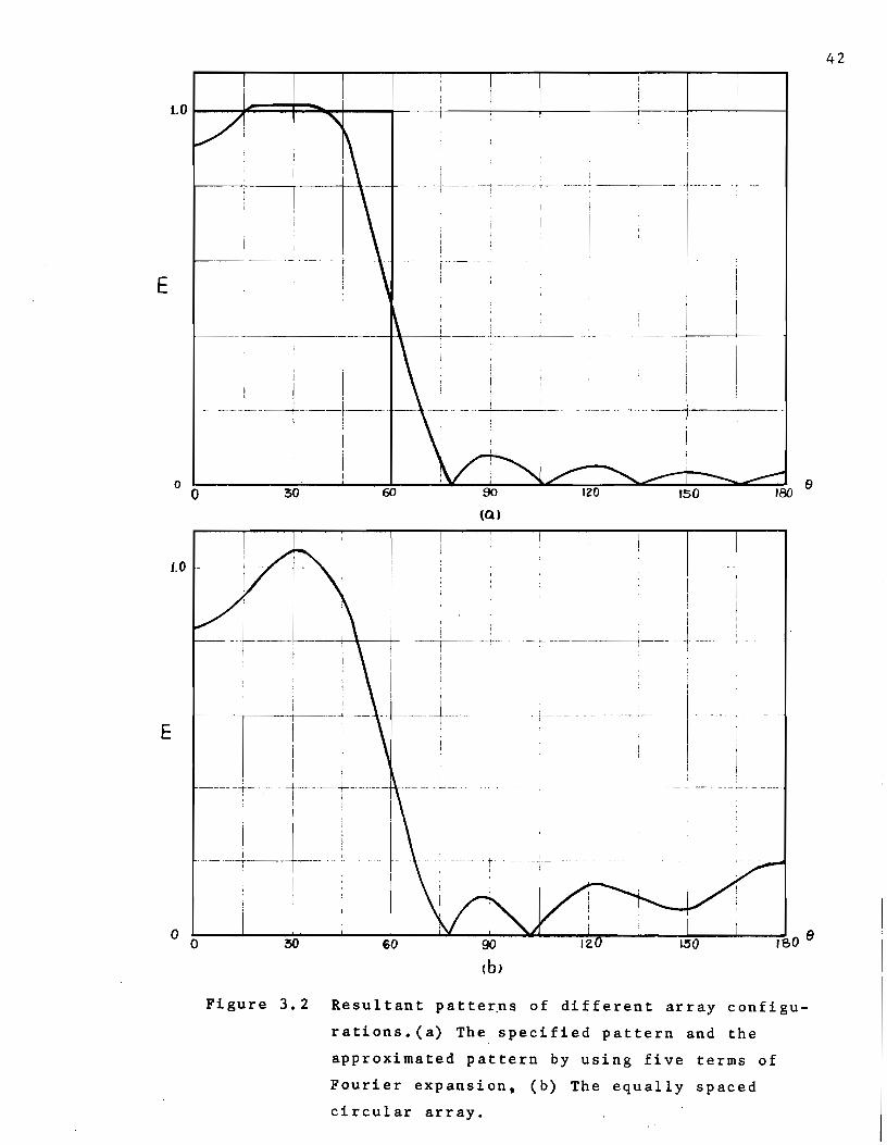
E

{Q)

Figure 3.2 Resultant patte~ns of different array configu­

rations.(a) The specified pattern and the

approximated pattern by using five terms of

Fourier expansion, (b) The equally spaced

circular array.

42

th an the specit.fi ed pat te rn, ne ver the 1 es s, the shape of the

main lobe is almost the same.

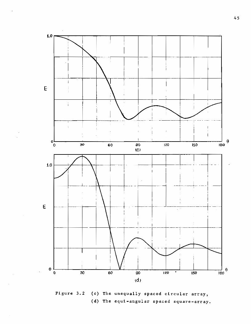
Configuration II: Let the elements be unequally distributed

along the circumference of the circle with d•J\/2, and let

the corresponding angular distribution (chosen arbitrarily)

0 Cl( 5 = 180 •

By solving (Eqs. 3.10) the relative amplitude can be obtained

as follows:

A = - 0.412 + j 1. 0441, Al = 0.1795 - j 1.580,: 0

A2 = 0.226 + j 0.03887, A3 = - 0.134 + j 0.0914,

A4 = 0.276 + j 0.114, A = 5 0.681 + j 0.291.

The resultant normalized pattern is shown in Figure 3.2c.

Although the resultant pattern is not as good as the pattern

of equally distributed array as shown in Figure 3.2b, it is

felt strongly that a pattern with small ripple and small minor

lobe level may be obtained by properly adjusting the spacing.

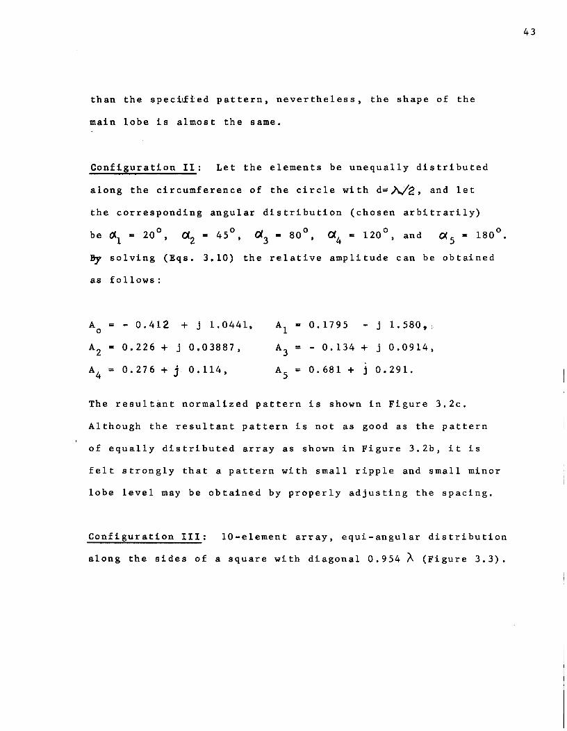
Configuration III: lü-element array, equi-angular distribution

along the sides of a square with diagonal 0.954 ~ (Figure 3.3).

43

As

Figure 3.3 10-element Array Equi-angu1ar Disttibution Along the Sides of a Square.

The distances from the centre 0 of the square to the

elements are

d = 0.477 >.. 0

dl= 0.342J\. • d2 = 0.379 À.

Then (Eqs. 3.7) become

44

••••• 3. 11

where m = 0, 1, 2, 3, 4 and 5. Solving (Eqs.3.11), the

following relative amplitude distributions are obtained.

A0

= -0.39995 + j 0.46603, A1 = 0.22487 - j Q.71552

A2 = -0.00452 + j ~.67279, A3 = 0.00452 - j 0.67279,

A4 = 0.22487 + j 0.71552, A5 = -0.39995 - j 0.46603.

E

E

0oL---------30~--------6~o---------g~o----~----~2~o---J----~,s~o--~----~~eo 9

(C)

oL---~--~----L---~~~--~----~--~--~----L---~--~ e 0 60 90 120 ISO 180

(d)

Figure 3.2 (c) The unequally spaced circular array,

(d) The equi-angular spaced square-array.

45

The resultant normalized pattern is shown in Figure 3.2d. It

will be noticed that the main lobe is quite close to that of

the approximate specified pattern of Figure 3.2a, but the

minor lobes are larger.

From the above examples, it is shown that (Eqs.3.7)

can be used in the synthesis of antenna arrays of a·.variety

of geometrical configurations. It is evident that the agreement

of the resulting pattern with the specified pattern depends on

the geometrical configuration concerned.

3.1.3 The Convergence of the Space-Phase Series

It should be noted that the above pattern synthesis

method is general in that it is not restricted only to arrays

of simple geometrical shape (i.e. circular or square arrays),

but is applicable also to arrays of arbit~ary shape as ,long as

the geometrical configuration of the array is symmetrical with

respect to 9=0. However, the number of elements used in

the array is not arbitrary. Since the derivation is based on

the series expansion of the space-phase term, therefore the

minimum number of terms used must be such that the space-phase

term ls. reasonably represented by the series expression.

Otherwise, a large~ror will be introduced.

example illustrates this.

The following

46

47

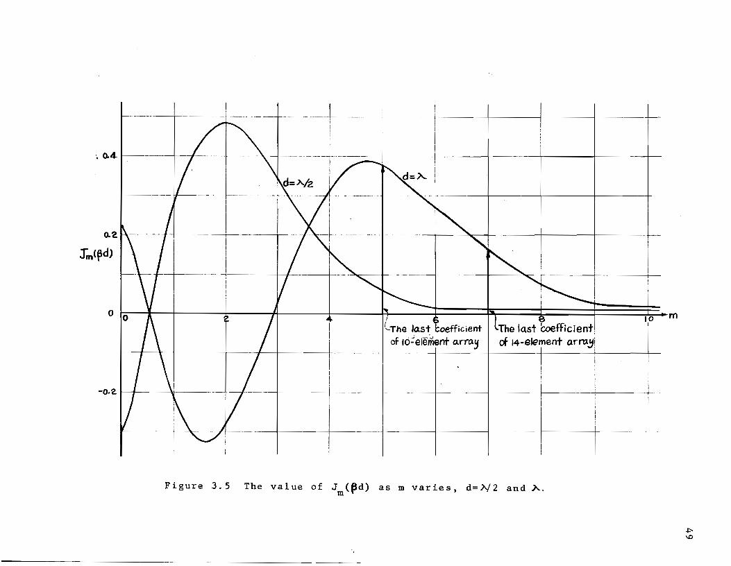
Consider a 10-~lement array with equally distributed

elements on the circumference of a circle of radius one

wavelength. (Eqs. 3 .10) become

Where m=O, 1 ••••• 5. The resultant normalized pattern is

shown in Figure 3.4a. Although the main lobe is almost the

same as shown in Figure 3.2a, nevertheless the minor lobe levels

are rather high. This can be shown to be due to the poor

approximation of the space-phase term:

Consider the space phase term

••••• 3. 12

Since, for the 10-element array, there are only six unknowns in the

amplitude distribution, then only six terms of the expansion

(Eq.3.12) are utilized. However, from Figure 3.5, it is evident

that the higher order coefficients are still appreciably large

and hence our approximation (Eq.3.12) of the space-phase term is

poor.

If a 14-element array is used, then the space-phase

term will be given by eight terms of the expansion (Eq.3.12)

and it can be seen from Figure 3.4 that the last coefficient

1.0

E

1.0

E

"" v !\ 1

.~ '

1 1

1 1

1 i ' 1 ; ! 1

. ·--··'

1 i

1

------ 1 1 !

1 1 1

1 \ 1 1 1 1 ' 1 1

!

\ ! 1 1

1 l --

i \ n~/1\Vv~/ 180 ° 120 !50

Figure 3.4 Resultant patterns of the circular array;

(a) 10-element array, (b) 14-element array.

48

-----4------~-~-- ·······-+--~-------~

0.2

Figure 3.5 The value of Jm(pd) as m varies, d=JY2 and À.

JT(2~) of the series (Eqs.3.12) is sufficiently small sa that

the higher arder terms can be neglected. The designed pattern

for the 14-element array is shown in Figure 3.4b and is

definitely far superior ta that of the lü-element array shown

in Figure 3.4a.

A general "rule-of-thumb 11 for the minimum number of

elements required for a circular array of any radius can be

obtained as follows. From the theory of Bessel functions,

Renee in the expansion 1

(Eq.3.12) terms of order higher than m may be ignored, where

m is the nearest integer larger than ~ d.

elements is then given by 2m.

The number of

3.2 Continuous Distribution and Circular Array.

It has been shown in Section 3.1 that any pattern which

can be approximated by a truncated Fourier series can, in

principle, be obtained from the curved array by adjusting the

amplitude distribution. If the closed curve is one of the

simple geometrie curves, such as the circle, ellipse etc.,

the antenna array is often discussed by using contin~ous

distribution. The equivalence between the discrete array and

the continuous distribution has been investigated by many

50

51

authors, and the method, which uses the amplitude of continuous

distribution as the envelope of the amplitude of equi-spaced

circular array has been used for a long time. Nevertheless,

the problem of minimum number of elements to replace the

continuous distribution has never been fully investigated. In

this section the relationship between the methods of continuous

distribution and the discrete array will be discussed.

3.2.1 Pattern. Synthesis by Using Continuous Distribution

Let the current be continuously distributed along the

circumference of a circle with radius d, amplitude A(a) and

phase ~(a). The far field pattern on the horizontal plane is

2n:

F(9)·J A(a)eJ(fd ••••• 3. 13

0

p

6=0, 01=0

Figure 3.6 Continuous Distribution with Amplitude A(ot) and Phase y(cc) •

52

If the amplitude is constant along the circumference and

the phase distribution is a linear function with total phase

shift 2m~, where mis any integer, then (Eq.3.13) becomes

21[

F(ll)• Am J ej (,dcos(ll-«)-mOtJda

0

••••• 3. 14

If the amplitude distribution is A cosm« , and the phase is m

constant, then the far-field pattern is

F ( 9) • 2 Jt € j mA J ( R d) c os m9 mm f"'

••••• 3. 15

If the specified pattern is symmetric with respect to the

axis 9=0. and ~t can be expanded as a eosine series, such that

00

S(9)= L m=O

S cosm9 m

••••• 3. 6

then the current distribution along the circumference will be

cosma" ••••• 3. 16

(Eq.3.16) is the solution for the continuous current distribution

provided that the series is convergent. In practice the number

of terms is usually finite for a reasonable design.

If the continuous distribution is represented by the

discrete array of 2N elements, then from (Eq. 3.16) the ampli-

tude of the nth element at the angular coordinate ex is n

53

Sm cosm<X

n ••••• 3. 17

The upper limit in (Eq.~3.17) is chosen to be equal toN. The

reason for this will be discussed in Section~3.2.2.

(Eq. 3.17) is equivalent to (Eqs.3.l0) if the 2N elements

are s .. paced equally along the ci r cumference. The proof is

given as follows.

Assuming 2N elements are used in the circular array, then

there are N+l equations in the form of (Eqs. 3.10)

••••• 3. 18

where m=O, 1, 2 ••• N. Since the elements are equally s~aced,

th en

and (Eqs.3.18) become:

m=O,l,2 ••• N.

Multiplying both sides of the above equations by cosmKa and

sqmming all the equations, we have

i {A0+2A1 cosmOl +2A2cos2m0l + ••• +ANcosNmOl} cosml<IX

m•O

N

54

-L cosmKOC ••••• 3. 19 m==O

N Si nee 2, cosmKCX =0

m=o

when NCX = 7t and ~ is integer. Therefore (Eq. 3.19) yields the

following:

N

Nl ~

AN = ~ m•o

s m cos mn()( ••••• 3. 20

' It is clear that (Eq.3.20) is the same as (Eq.3.11) except for

a constant multiplying factor which has no consequence on the

pattern.

3.2.2 The Upper Limit of m

It has been assumed in (Eq.3.17) that the upper limit of

m is N where N is half the number of elements. It will be shown

that this upper limit need only beN and not higher. To do this,

55

suppose the upper limit is N+l, then from (Eq.3.17) the

amplitude of the nth element is

N+l -m

A n

1 = 2:n: 2:: j cos mor

n ••••• 3. 21

m=O

Since there are 2N elements equally distributed on the circumfer-

ence then

and hence cos(N+l)Ql = cos(ll}{+()() = cos(n7C-Cif) n n n

= cos ( N -1) CXn ••••• 3. 22

With the help of (Eq.3.22), the last term of (Eq.3.21) i.e. the

term m=N+l, is reduced to the form

cos(N+l)<Xn = j-(N+l)

cos (N-1)0( n

In other words, the term m=N+l can be combined with the term

m=N-1 and in general terms of order higher than N can be

combined with terms of order correspondingly lower than N.

E

GO 90 120

Figure 3.6 Resultant pattern of 14-element array with abnormal

amplitude~disttibution.

Renee the upper limit need only be N. In fact if the upper

limit exceeds N, the pattern will degrade as illustrated by

' the following example:

The amplitude distribution of a 14-element equ~angular

circular array is given by (Eq.3.17)

A n

1 --2n j

-m

If the specified pattern is the same as in Section 3.1.2, and

the radius d is one wavelength, then the resultant pattern will

be the same as shown in Figure 3.3b.

includes two extra terms:

1 27t

9

~ m=8

j -m s

m

If the expression of A n

the resultant pattern is shown in Figure 3.6. Comparing with the

pattern ~n Figure 3.3b it is found that the minor lobe level

in Figure 3.6 increases by a large amount.

3. 3 Circular Array of AnLsotrQpi.c · Element;s

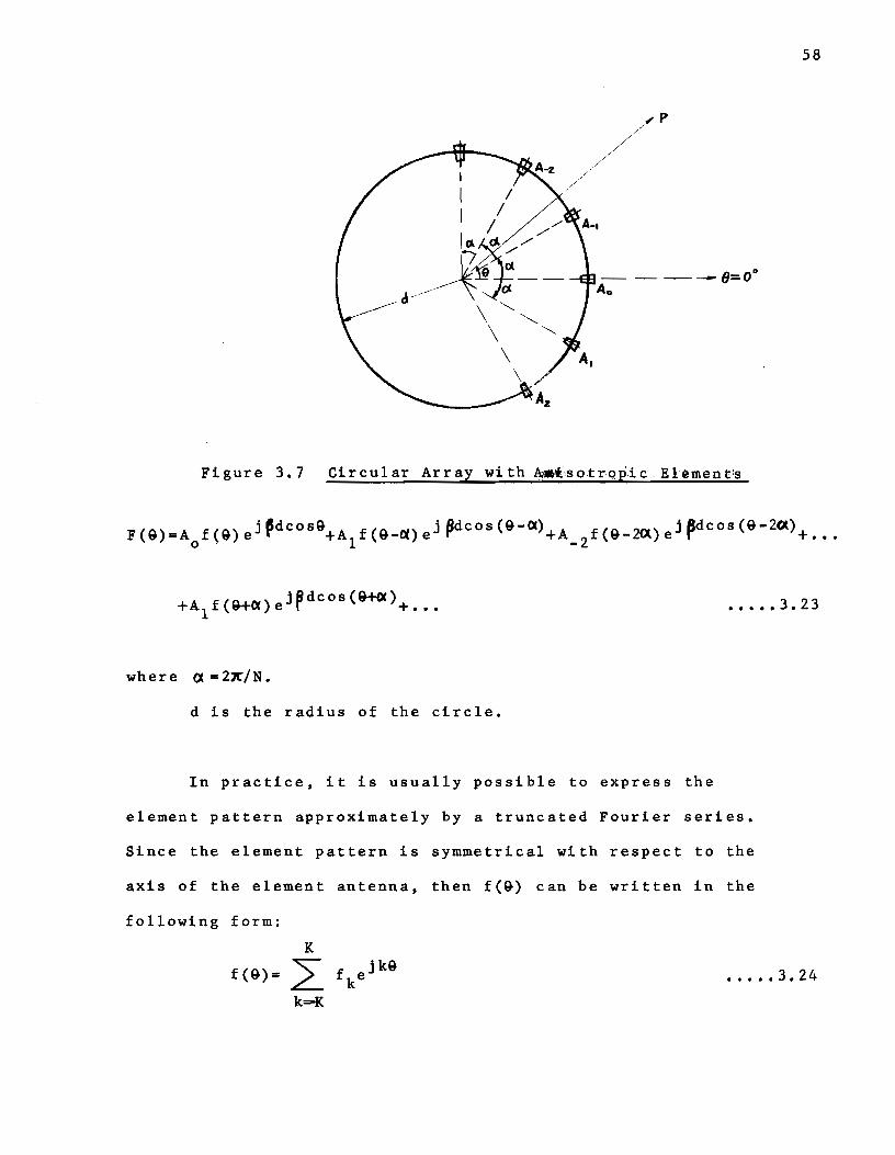
If the element pattern of each antenna is f(~), the

far-field pattern of an N-element equally spaced circular

array with amplitude distribution A is given by (Eqs.2.1 and n

2.2) whereby each term is multiplied by its respective pattern f.

57

.,-P

-----8=0" Ao

Figure 3. 7 Circular Array wi th ~tsotrqp.ic .Element;s

58

••••• 3. 23

where CX = 27C/N.

d is the radius of the circle.

In practice, it is usually possible to express the

element pattern approximately by a truncated Fourier series.

Since the element pattern is symmetrical with respect to the

axis of the element antenna, then f(9) cau be written in the

following form:

K

f(9)= L k-K

••••• 3. 24

where ~k=fk. By using the mathematical identity {Eq.3.2)

and with the symmetric condition A =A , the far-field pattern -n n

of the array becomes:

59

••••• 3. 2 5

Since the antenna system is symmetrical with respect to

the axis 9=0, th en the final exp res si on of the far -field pat t.ern

is in the following form:

1!(9)=± fA0

J!m+2A1 •Fm"cosmOC +2A 2 •J!m"cos2mfX+ •••

m•O

••••• 3. 26

where F m In fact (Eq.3.26) is

in the same formas (Eq.3.4) when d0

=d1=d

2= ••• Although the

constants Fm are more complex than the constants Jm(Pd} in the

circular array with isotropie sources, nevertheless the series

Fm is just an algebraic combination of fk and Jp(~d) and it

suffers the same defects as the series Jm(Pd) in the

circular array, i.e. slow convergence of the series. Because

of this it is impractical to apply the method to the design

of circular arrays at microwave frequencies using conventional

aperture antennas as the an~sotro~ic ·elemerits. The limitation,

however, is purely physical as discussed below.

In Section 3.1, it has been shown that for the

circular array with equally spaced isotropie elements the

minimum number of elements required is the nearest integer larger

The length of the circumference is equal to 2nd, and

hence the spacing between each element is approximately equal

to 2~d/2~d or Â/2. If we stipulate that the convergence of

Fm and Jm(~d) be roughly the same then it is reasonable to

expect that the number of elements in the circular array with

ani~tropic sources will be approximately the same as that with

isotropie sources, and therefore the spacing between each

element will also be equal to Â/2. This spacing is too small

for most aperture antennas when used as the antenna element

in the anisotrop1c arra,y •• However, this does not rule out

the possibility of using aperture antennas for the circular

array. It only means that the above theoretical approach

60

cannot be applied. When theory fails, it is perhaps natural

to aonduct some simple experimente to see if it is possible

to obtain some idea as to the best future approaah.

61

IV. EXPERIMENTAL STUDY OF THE CIRCULAR ARRAY WITH~NlSOXROPIC

ELEMENTS.

4.1 Introduction

In the previous chapter, it has been shown that the series

expansion method fails if aperture antennas such as horns or

parabolic reflectors are used as the elements for the circular

array. Since no other analytical method seems to be readily

available, it may be useful to investigate experimentally the

characteristics of the circular array wi th ani'.s:o:t-rqpi~ 'e.leme.n:t:s

to see if a correct approach could be devised. In this chapter,

the far-field pattern of a set of horns which are equally

distributed along the arc of a circle will be measured and

based on the measured results, several conclusions will be

drawn.

4.2 Experimental Arrangement

The problem of far-field pattern measurement consista of

two parts: the site of the transmitting and receiving antennas,

and the detecting equipment. For a small aperture antenna

system with moderate beamwidth, two factors have to be

considered for the choice of a site: (a) the distance between

the transmitting and receiving antennas and (b) the freedom

from ground and other reflections.

62

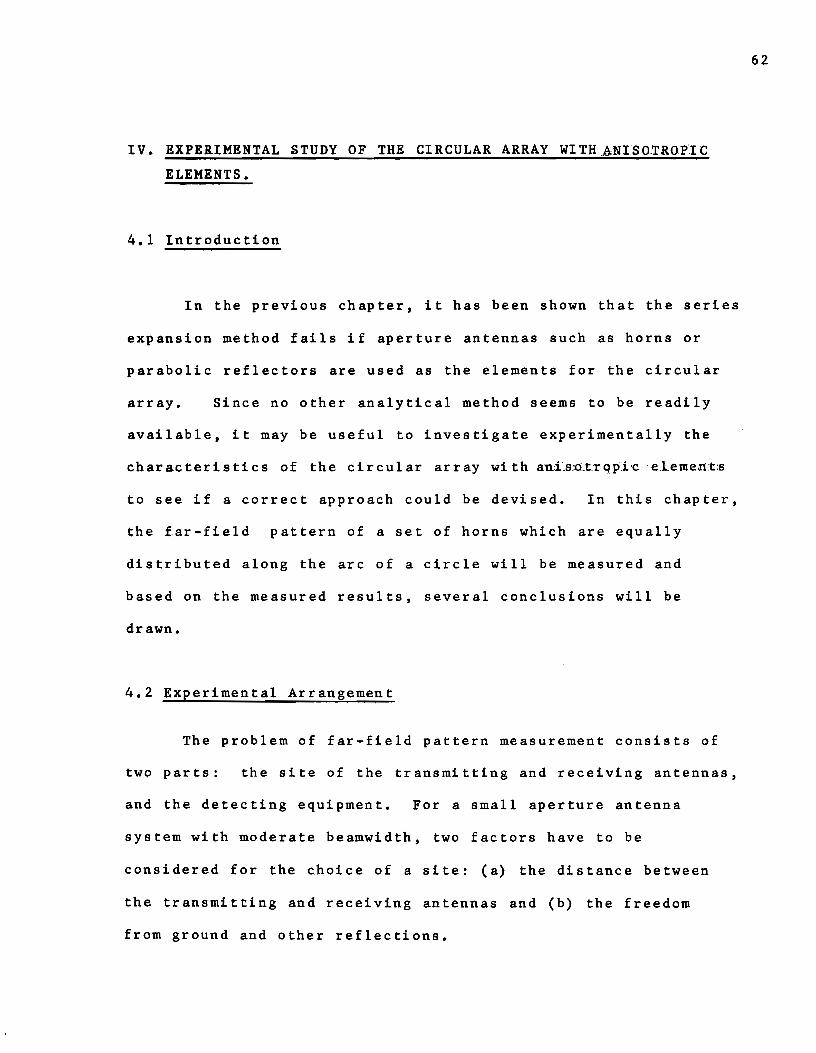
It is well known that to approximate a plane wave

condition the distance R required between the transmttting and

2 receiving antennas must be larger than or equal to 2D /À where

Dis the aperture dimension of the tested antenna and~ is·

the wavelength of the radiation, both measured in the same

units. For the circular array, the aperture may be defined

as the largest distance measured in a straight 1ine between

any two of the antennas in the array. For instance, if the

antennas are distrmbuted on the arc which is 1arger than the

ha1f circle, the aperture will sti11 be equa1 to only the

diameter of the circle. In the fol1owing measurements, the

largest aperture of the tested antenna system is approximately

equa1 to 46 cm and the operating frequency is 9.34 KMc/s.

(X-baad), i.e. ~-3.2/cm, thus

2x46 2 R ~ • 13.2 meters.

? 3.21

In Figure 4.1, it is shown that the actua1 distance between the

transmitting and receiving antennas is approximately equal to

63

17 meters, which means that the site satisfies the phase criterion

for the far-field measurement •.

In the measurement of a far-field pattern, complete

freedom from ground and other reflections is impossible.

However, the ref1ections can usually be minimized by c~rtain

methods, such as tilting one of the antennas upwards so that the

r ' l

1 e' lfl .....

~~~~~~~~~~~~~-~~~--~'.-. ~~~~~~~~~~~~~~~~, APPROX. 40M

64

ABOVE GROUNO

Figure 4.1 The physical dimensions of the transmitting

and receiving antenna towers.

Klystron Power f---Supply

Tested

Antenna

Power

Di vider

Rotary

Joint

Isolator

V-55 B

Klystron

Parabolic

Reflector

Crystal

De tee tor

Rota ting

Table

A. F.

Amplifier Il Il

D. c. Selsyn

Mot or Mo tor

1 f Intensity

Variable Position o.c. Power

Supply Indicator Indicator

Figure 4.2 Block diagram of the equipment arrangment.

Single line representa electrical connection

and double line representa mech~ical coupling, A

first null of the vertical beam points towards the reflection

point, or placing absorption screens or diffracting edges

halfway between the two sites. Since the test range is

located on the roof of the highest building on the campus,

there are no reflections from surrounding objecta. The heights

of both antenna towers is 4.3 meter above the roof, and both

the transmitting and receiving antennas are highly directive

in the vertical plane, so that groundward radiation from the

transmitting antenna and the groundward reception of the

receiving antenna are very small.

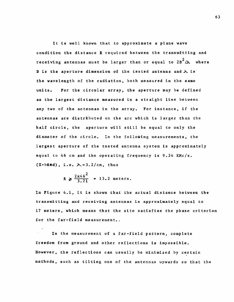
The detecting equipment consista of two parts; the

position indicator and the crystal detector. The position

indicator is synchronized to the rotating table by selsyn

motors. The crystal detector is an ordinaryone used in X-band.

Its output is connected to a VSWR meter which is used as

an a-f amplifier and intensity indicator. The crystal detector

and VSWR meter combination are calibrated by means of the r-f

substitution method. The patterns obtained here were measured

manually, since a fully automatic recording system was not

yet completed.

The source of r-f power is a modulated reflex klystron

V-55B with an output of 240 mw. The radiated frequency is

9.34 KMC. A block diagram of the equipment is shown in

Figure 4.2.

65

66

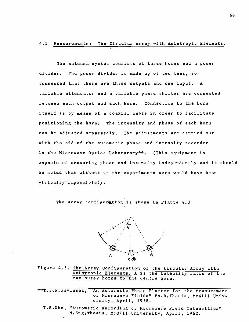
4.3 Measurements: The Circular Array with Anistropic Elements.

The antenna system consists of three horns and a power

divider. The power divider is made up of two tees, so

connected that there are three outputs and one input. A

variable attenuator and a variable phase shifter are connected

between each output and each horn. Connection to the horn

itself is by means of a coaxial cable in order to facilitate

positioning the horn. The intensity and phase of each horn

can be adjusted separately. The adjustments are carried out

with the aid of the automatic phase and intensity recorder

in the Microwave Optics Laboratory**· (This equipment is

capable of measuring phase and intensity independently and it should

be noted that without it the experiments here would have been

virtually impossible!).

The array configur,tion is shown in Figure 4.3

~~\ / : \. ,' 1 1 \ /

1 \ ' ,..r

A --~~ . .ffi ..... -----~ odb

Figure 4.3 •. The Array Configuration of the Circular Array with Anistropic Elements. A is the intensity ratio of the two outer horns to the centre horn.

**T.J.F.Pavlasek, "An Automatic Phase Plotter for the Measurement of Microwave Fields" Ph.D.Thesis, McGill Univ­ersity, April, 1958.

T.S .. Kho, "Automatic Recording of Microwave Field Intensities" M.Eng~Thesis, McGill University, April, 1962.

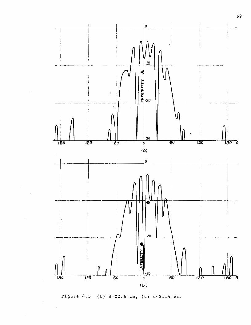
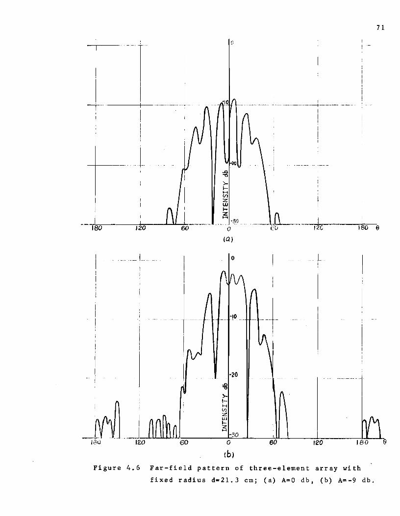
Two series of measurements were carried out, the phase of the

horns being kept equal in both cases. In the first case the

amplitude distribution of the array was varied with the radius

of the circle, or the arc, kept constant. The measured patterns

with d=21.3 cm and variable A are shown in Figures 4-6. In

the second series of measurements the radius d was varied but

the amplitude distribution was kept constant at (-6 db, 0 db,

-6 db). The measured patterns are shown in Figures 4-5. From

these two series of measurements, the following conclusions

can be drawn:

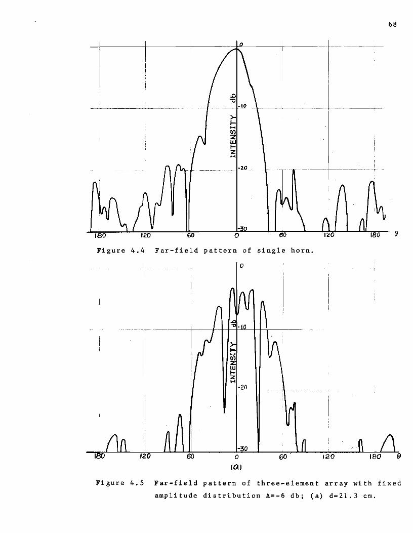
(a) The ripples at the main beam increase as d increases.

(b) The ripples at the main beam increase as A increases.

(c) There are always two very low minimum points in the main

67

bearn, the beam width between these two points being

approximately constant except for the cases of d=40.4 cm and

A=O db.

(d) The beam width of the resultant pattern is slightly larger

than the bea~~idth of the element antenna.

(e) The number of ripples is constant except for the cases d=40.4cm

and A=O db.

The main disadvantages of the resultant pattern is the violent

fluctuations at the main lobe. From the results, it seems

possible that the fluctuating effect can be reduced by

-+------+-----+---±"----t----t----1-

180 60

>­~ ..... tl} 2 w 1-z H

---- ----------- -------- - :lO. ---

- 0 0

Figure 4.4 Far-field pattern of single horn.

0

-30 0

(C\)

1

1

i

120

68

e

Figure 4.5 Far-field pattern of three-element array with fixed

amplitude distribution A=-6 db; (a) d=21.3 cm.

1-1-4 [1) z w ...

0

~-20

69

__ .[ __

...... ~--L....L..--:-*.;:::-----'-~~--.....L-~-3::..::::0_.L-._~__......__"I?!;;:;----fr~ o ISO e tb)

0

(C)

Figure 4.5 (b) d=22.6 cm, (c) d=25.4 cm.

8

A--•>no•

1

!

---~·-· 1

1

i 1

(1 f'l

ni\ n n 1 180 1 20

-r-- 1

i 1 1 1

····t .. 1 -"''""-·

1

1

1 1

...

~ " J 1

1 1 180 120

n

1 ·-------~~--~··-·

Q

.

" rv

..

60

J

1 1

1

1

1

! 1

1

60

"' r,

,

·10

-2()

~ >-.... ..... Il)

z w 1-:z H

-30 0

0 .. ,.

.- ... ::-IC

l-2t ...Q

"0

>-..... ..... Cil z I.U 1-z ....

-3D 0

te,

70

1 - 1 -

,.,

r\ --·-

' 1

1

1

U1 1 t

·1 1 1 1 1

·---- ------1 1

1

1 1

f ~~ \1\ fl 1\ A

60 120 ISO fi

1 ~ . i i

1 1

1

1

'

IJ'I1

__ _lo ~

' :

60 120 180 \J

Figure 4.5 (d) d=27.7 cm, (e) d=40.4 cm,

1 -r--- -----+

>-1-H (/) z w .... z ......

71

20 -· j

-~()

0 12C tao e (Q)

0 - J __ !

·20

=@ )-

1 ,_

~--~~~-~~~0~~~~~ IGù 120 60 0 60 120

<b> Figure 4.6 Far-field pattern of three-element array with

fixed radius d=21.3 cm; (a) A=O db, (b) A=-9 db,

... ~ 1-2 1-1

72

0

--~~~----~----~~~--------~-3~0------~~~------~--------~~9 120 0 60 120 180

180 120 60

(Ç)

_0 __ ~~-

.0 "0

).. ... .... Il) z

i

!

-20

Figure 4.6 (c) A=-12 db, (d) A=-15 db.

--------·-1 l 1

180

reducing the radius d, but d is limited by the physical dimension

of the element antenna. Although the resultant pattern is no

better than the pattern of a simple horn, however, there exista

the possibility of steering the resultant pattern of the array

by varying the amplitude of è~ch antenna. For instance, for

the four-element array if the geometrical configuration is

defined.'.by 9=30'0

and d=21.3 cm and thé ampÙtude distrlbution

is (-"6· db, ·o d·b, ..,'6db) w·ith one edge element non-excited, the

resultant pattern is shown in Figure 4.7a. If the amplitude

distribution changes to (-9.5 db, 0 db, 0 db, -9.5 db), the

resultant pattern is shown in Figure 4.7b. It is evident that

the direction of the main pattern is changed as expected.

This fact should form the basis of an extensive experimental

investigation.

73

V. CONCLUSION

Although the problem of pattern synthesis of antenna

arrays has been tackled for several decades, it is surprising

that only few successful methods are available. In particular,

74

the problem of the unequally spaced linear array, of the curved

array and of the circular array wi th anLs:d:trop.i-c re.lement:,s have

seldom been discussed in the literature. It has been the purpose

of this thesis to investigate possible methods of pattern

synthesis for the antenna arrays mentioned above. Sever al

methods have been examined but further research is required.

Hitherto, the optimum pattern of an antenna array has

been designed for the equally spaced array by adjusting the

amplitude distribution. In this work, a new method of optimum

pattern synthesis has been devised. It has been shown that the

optimum pattern of a linear array with fixed amplitude

distribution can be obtained by adjusting the antenna spacing.

The relationship between the space distribution and the

amplitude distribution has also been discussed by means of an

eKample. The rigorous mathematical analysis is extremely

difficult and needs further development.

The author has developed a pattern synthesis method for

the general curved array with isotropie sources. The method

ii applicable to any array configuration as long as the array

is symmetric with respect to the pattern axis. It is believed

that for a fixed number of elements and a specified pattern

there is an optimum array configuration which will result in the

best agreement between the resulting pattern and the specified

pattern. The series expansion method is unworkable if applied

to arrays with ani.s'Otropic .source:s_, due principally to the physical

size of such antennas. A simple experiment has been performed

to substantiate certain salient points of such arrays.

The ultimate objectives for the present study of pattern

synthesis for antenna array is to solve the problem of electronic

0 steering of the antenna beam through 360 • If a suitable

element antenna can be obtained for the circular array of

ani.sotr.op.ic ·sour.ces,, it is quite possible to achieve a scanning

pattern by v~rying the amplitude of each element. Alternively,

other theoretical approaches should be investigated such as

expansion of the space-phase term and the specified pattern by

some other series that have better convergence properties

than the Bessel-Fourier series used in this work. Certainly

the proDlem is a very difficult one and is no-where near a

,EiOlution. It is hoped, however, that the work here is a

small contribution towards that end.

75

BIBLIOGRAPHY

Books

1. H.Jasik, "Antenna Engineering Handbook", McGraw-Hi11, New York, 1961.

2. E.C.Jordan, "E1ectromagnetic Waves and Radiating Systems", Prentice-Ha11, New York, 1950.

3, J.D.Kraus, "Antennas 11, McGraw-H111, New York, 1950.

4. B..W.P.King, "The Theory of Linear Antennas", Harvard University Press, Cambridge, Massachusetts, 1956.

5. S.A.Sche1kunoff and H.T.Friis, "Antenna Theory and Practice", John Wi1ey & Sons Inc., New York, 1952.

6. S.Si1ver, "Microwave Antenna Theory and Design", McGraw-Hi11, New York, 1949.

76

7. J.Stratton, "E1ectromagnetic Theory", McGraw-Hi11, New York,1941.

Linear Arrays and Line Sources

8. C.C.A1len, "Radiation Patterns for Aperture Antennas with Non-Linear Phase Distributions", I.R.E. Convention Record, Part 2, p.9, 1953.

9. W.H. von Au1ock, "Properties of Phased Arrays", Proc.I.R.E., Vol.48, p.1715, October, 1960.

10. P.A.Bricout, "Pattern Synthesis Using Weighted Functions", I.R .. E. Trans., Vol. AP-8, p.441, Ju1y, 1960.

11. G.H.Brown, "Directional Antennas", Proc.I.R.E., Vol.25, p.78, January. 1937.

12. G.H.Brown, "Pattern Synthesis - simplified methods of array design to obtain a desired directive pattern", R.C.A. Rev., Vo1.20, p.398, September, 1959.

13. J.Brown, "The Effect of a Periodic Variation in the Field Intensity across a Radiating Aperture", J.I.E.E. (London), Vo1.97-III, p.419, November, 1950.

14. J.L.Brown Jr., and R.O.Row1ands, "Design of Directional Arrays", J.Acoust. Soc.Am., Vol.31, p.l638, December, 1959.

77

15. H.G.Booker and P.C.Clemmow, "The Concept of an Angular Spectrum of Plane Waves, and its Relation to that of Polar Diagram and Aperture Distribution", J.I.E.E.(London), Vol.97-III, p.ll, January, 1950.

16. D.K.Cheng and M.T.Ma, "A New Mathematical Approach for Linear Array Analysis", I.R.E. Trans., Vol.AP-8, p.255, May, 1960.

17. W.A.Cumtning, "A Nonresonant Endfire Array for V.H.F. and U.H.F.", I.R.E. Trans., Vol.AP-3, p.52, April, 1952.

18. L.H.Dawson and N.M.Rust, "A Wideband Linear-array Aerial", J.I.E.E. (London), Vol.93-IIIA, p.693, 1946.

19! A.S,Dunbar, "On the Theory of Bearn Shaping", J.Appl.Phys., Vol.23, p.847, August, 1952.

20. A.J.Ebel, "Directional Radiation Patterns", Electronics, Vol.9, p.30, April, 1936.

21. R.M.Foster, "Directive Diagrams of Antenna Arrays", B.S.T.J., Vol.5, p.292, October, 1926.

22. F.K.Goward, "An Improvement in Endfire Arrays", J.I.E.E., Vol.94-III, p.415, November, 1947.

23. W.W.Hansen and L.M.Hollingsworth, "Design of Flatshooting Antenna Arrays", Proc.I.R.E., Vo1.27, p.l37, February, 1939.

24. W.W.Hansen and J.R.Woodyard, "A New Principle in Directional Antenna Design", Proc.I.R.E., Vo1.26, p.333, March, 1938.

25. R.F.I;larr:i,.ngton, "Sidelobe Reduction by Nonuniform Element Spacing'', I.R.E. Trans., Vol.AP-9, p.l87, March, 1961.

26. C.W.I;larrison Jr., "A Note on the Characteristics of the Two Antenna Array", Proc. I.R.E., Vol.31, p.75, February, 1943.

27. A.Heilmann, "The Optimum Current and Field Distribution for Bro~dside ·and Endfire Radiators with Continuous Illumination", Nachrich, Vol.9, p.l, January, 1956.

28. J.N.Hines, V.H.Ramsey and T.E.Tice, "On Design of Arrays", Proc. I.R.E., Vol.42, p.l626, August, 1954.

29. M.Hc;>ffman, "The Utility of the Array Pattern Matrix for Linear Array Computations", I.R.E. Trans., Vol.AP-9, p.97, Jan u ar y, 19 61.

30. D.D.King, R.F.Packard and R.K.Thomas, "Broadband Steerab1e Linear Arrays", E1ectronic Communications, Inc., Timonium,

78

Md., prepared for AFCRC, Contract AF19(604X-5234, October, 1959.

31. H.E.King, "Directivity of a Broadside Array of Isotropie B.adiators", I.B..E .. Trans., Vol.AP-7, p.l97, April, 1959.

32. J.D.Kraus, "Antenna Arrays with Closely Spaced Elements", Proc, I.R.E., Vol.28, p.76, February, 1940.

33. A.Ksienski, G.G.Comisar and O,R.Price, "Logica1 Pattern Synthesis", I.R.E. WESCON Convention Record, Part 3, p.32, 1959.

34. A.Ksienski, "Maximally Flat and Quasi-Smooth Sector Beams", AFCRC-TN-59-581, Scientific Rept. 3508, Hughes Aircraft Co., California, July, 1959. I.R.E.Trans., Vol.AP-8, p.476, September, 1960.

35~ A.Ksienski,."Derivative Control in Shaping Antenna Pattern", AFCRC-TN-60-110, AD-233091, Scientific Rpt. 2358/6, Contract AF19(604)-3508, Hughes Aircraft Co. California, September, 1959.

36. A.Ksienski, "Equivalence between Continuous and Discrete Arrays", AFCB.C-TN-60-1104, Scientific Rpt. 3508/7, Contract AF19(604)-3508, Hughes Aircraft Co. California, April, 1960. J.Cand. Phys., Vol.39, p.335, February, 1961,

37. A.Ksienski, "Interpolation Techniques applied to Pattern Synthesis", AFCB.L-TN-60-1178, Scientific Rpt. 3508/8, Contract AF19(604)-3508, October, 1960.

38. A.Ksienski, "Synthesis of Nonseparable Two-dimensiona1 Pattern by means of Planar Arrays", I.R.E. Trans, Vol.AP-8,p.224, Mar ch, 19 60.

39. E.A.Laport, "Radiation Pattern Synthesis", R.C.A.Rev., Vol.l4, p.533, December, 1953.

40. J.B.Lewis, 11 Use of Folded Monopoles in Antenna Arrays 11,

I.R.E. Trans., Vol.AP-3, p.122 1 July, 1955.

41. J,R.Lignon, "Directivity of Endfire Arrays of Isotropie Antennas", An.Acad.Brasil Ciênc., Vol.28, p.439, December, 1956.

42. R.L.Matting1y, "Nonreciprocal Radar Antenna:, Proc.I.R.E., Vo1.48, p.795, April, 1960.

43. E.B~Moullin, usingle Method for Observing Current Amplitude and Phase Relations in Antenna Arrays", J.I.E.E. (London), Vol.91-III, p.23, March, 1944.

79

44. H.Page, "Horizontal Dipole Transmitting Arrays", J.I.E.E.(London}, Vol.92-III, p.68, June, 1945.

45. V.L.Pokrovskii, "A General Method for Optimum Spacing of Linear Aeria1s", Dokl. AN USSS&, Vol.l38, p.584, May, 1961. Soviet Physics • Dok1ady (USA), Vo1.6, p.435, November, 1961.

46. O.R.Price, "Reduction of Side-1obe Leve1 and Beam Width f•r Receiving Antennas", Proc.I,R,E. Vo1.48, p.1177, June, 1960,

47. R.L.Pritchard, "Maximum Directivity Index of a Linear Point Array", J.Acoust., Soc4Amer., Vol.26, p.l034, November, 1954.

48. li.P.Raabe, "Antenna Pattern Synthesis of the most Truthfu1 Approximation", I.R.E. WESCON Convention Record, Vo1.2, Part I, p.l78, 1958.

49. A.R.Rumb1e, "Directiona1 Array Field Strength", E1ectronics, Vo1.10, p.16, August, 1937.

50. S.S.Sandler, "Some Equiva1encies between Equa11y and Unequally Spaced Arrays", I.R.E. Trans., Vol.AP-8, p.496, September,l960.

51. S.A.Sche1kunoff, "A Mathematical Theory of Linear Arrays", BSTJ, Vol.22, p.80, January, 1943.

52. O.Schmidt, "Aerial Arrays with Hori~ontal Beams Without Sidelobes", Bull.Schweiz. Elektrotech Ver;., Vo1.38, p.15, 1947.

53. A.H.Secord and W.V.Tilston, "A New Célinear Anteâna Arrây", I.R.E. Trans., Vol.VC-9, p.3l, August, 1960.

54. H.E.-Shanks, "A new Method of Pattern Synthesis fer Linear Arrays", AFCRC-TN-59-568, Scientific Rpt. 3508/1, Contract AF19(604)-3508, Hughes Aircraft Co., California, July, 1959.

55. B.E.Shanks, "A Geometrical Optics Method~6f:Pâttern Synthesis for Linear Arrays", I.R.E. Trans., Vol.AP-8, p.485, September, 1960.

56. J.P.Shelton and K.S.Ke1leher, "Multiple Beams for Linear Arrays", I.R.E. Trans., Vol.AP-9, p.l54, March, 1961.

57. G.,C.,.Southworth, "Certain Factors Affecting the Gain of Directive Antennas", BSTJ, Vol.lO, p.63, January, 1931.

58. T.T.Taylor and J.R.Whinnery, "Application of Potential

80

Theory to the Design of Linear Array", J.Appl.Phy~., Vol.22, p.,19, January, 1951.

59. T.T.Taylor, 11 Design of 1ine-source Antennas for Narrow Bandwidth and Low Side1obes", I.R.E. Trans., Vd.AP-3, p.l6, January, 1955.

60. S.Teitelbaum, "On Some Problems of the Theory of Highly­Directive Antenna Arrays"~ Bull.Acad. Sei. USSSR, Vol.lO, p.285, 1946.

61. H.Unz, "Linear Arrays with Arbitrarily Distributed Elements", Electronics Res.Lab., University of California, Berkeley, Ser.No.60, Issue No.l68, November, 1956.

62. G.J.Vogel, "Phased Arrays", Rome Air Development Centre RADk!­TR-59-135, November, 1959.

63. C.B.Watts Jr., "Simultaneous Radiation of Odd and Even Patterns by a Linear Array", Proc.I.R.E., Vol.40, p.l236, October, 1952.

64. N.Wells, 11 Quadrant Aerial", J.I.E.E. (London), Vol.91-III, p.l82, 1944.

65. !.Wolf, "Determination of the Radiation System which will Produce a Specified Directional Characteristic" Proc.I.R.E., Vol.25, p.630, May, 1937.

66. P,.M.Woodward, "A Method of Calculating the Field over a Plane Aperture required to Produce a Given Polar piagram", J.I.E.E.(London), Vo1.93-IIIA, p.1554, 1946.

67. P.M.Woodward and J.D.Lawson, " A Irheo:r:enical Precision with which an Arbitrary Radiation Pattern may be . Obtained from a Source of Finite Size". J.I.E.E.(London)

68. R.F.H.Yang, "Optimum Element Spacing of Uniform Broadside Arrays", Wireless Engr., Vol.32, p.l55, April, 1955.

69. J.L.Yen, "On the Synthesis of line-sources and Infinite St:rip!""source_.", I .. B..E .. Trans .. , Vol .. AP-5, p .. 40, January,l957.

81

Tschebyscheff Distribution

70. l<.Barbiere, "A Method for Ca1cu1ating the Current Distribution of Tschebyscheff Arrays", Proc. I.R.E., Vo1.40, p.78, January, 1952.

71. A.B1ock, R.G.Medhurst and S.D.Pool, "A New Approach to the Design of Super-Directive Aeria1 Array", Proc.I.E.E., Vol.lOO-III, p.303, September, 1953.

72. J.L.Brown Jrd., "A Simplified Derivation of the Fourier Coefficients for Chebyshev Patterns", Proc. I.E.E., Vol.105-C, p.107, November, 1958.

73. L.B.Brown and G.A.Sharp, "Tchebyscheff Antenna Distribution, Beamwidth and Gain Tables", Naval Ord.Lab., Corona, California, NAV-ORD Rpt. 4629, 1958.

74. C.L.Dolph, "A Current Distribution for Broadside Arrays which Optimizes the Relationship between Beam Width and Side­lobe Level", Proc. I,R.E., Vol.34, p.335, June, 1946.

75. R.H.Ouhamel, "Optimum Patterns for Endfire Arrays", Proc.I,R.E., Vol.41, p.652, May, 1953.

76. S.Herscovici, "Design of Linear Arrays giving Optimum Radiation Pattern"~ Annales de Radioelectricite, Vol.9, p.352, October, 1954.

77. G.J. van der Maas, "A Simplified Ca1culation for Dolph­Tschebyscheff Arrays", J.Appl.Phys, Vol.25, p.l21, January, 1954.

78. O.R .. Price and R.F.Hyneman, "Distribution Functions for Monopu1se Antenna Difference Patterns", I.R.E. Trans., Vol. AP-8, p.567, November, 1960.

79. R.L.Pritchard, "Discussion on Optimum Patterns for Endfire Arrays", I.R.E. Trans., Vol.AP-3, p.40, January, 1955.

80. M.L.Reuss Jr., "Some Design Considerations Concerning Linear Arrays Having Dolph-Tchebyscheff Amplitude Distributions", Naval Res.Lab., U.S.A., N.R.L. Rpt. 5240.

81. D.R.Rhodes, "The Optimum Linear Array for a Single Main Beam", Proc. I.R.E., Vol.41, p.793, June, 1953.

82. J.Riblet, "Discussion on Dolph's paper", Proc. I.R.E., Vo1.35, p.489, May, 1947.

83. H.E.Salzer, "Discussion on Barbiere's paper", Proc. I.R.E., Vol.42, p.1021, June, 1954.

84. G.Sinclair and F.V.Cairns, "Optimum Patterns for Arrays of Nonisotropic Sources", I.R.E. Trans., Vol.AP-1, p.50, February, 1952.

82

85. I.F.Sokolov and D.E.Bakman, "Optimum Linear Co-phased Ae:i:ials with Continuous Current Distribution", Radiotekh.Elektron., Vo1.3, p.46, January, 1958.

86. R.J.Stegen, "Excitation Coefficients and Beamwidths of Tschebyscheff Arrays", Proc. I.R.E., Vol.41, p.1671, November, 1953.

87. B. van der Pol and T.J<.Wayers, "Tschebyscheff Polynomials and their Relation to Circular Functions, Bessel Functions and Lissajous Figures", Physica, Vol.l, p.78, 1933.

88, .~N.Yaru, "A Note on Supergain Antenna Arrays", Proc. I.R.E., Vo1.39, p.l081, September, 1951.

Circular Arrays '69. V.W.Bolie, "Beam Phasing in a Circular Array of Vertical

Antennas", Proc. I.R.E., Vo1.47, p.90, January, 1959.

90. P.S.Carter, C.W.Hanse11 and N.E.Landenblad, "Development of Directive Transmitting Antennas by R.C.A. Communications

:·rnc." Proc. I.R.E., Vol.19, p.1773, October, 1931.

91. P.S.Carter, "Antenna Arrays Around Cylinders", Proc. I.R.E., Vo1.31, p.671, December, 1943.

92. L.J.Chu, "Physical Limitations of Omnidirectional Antennas", J.Appl.Phys., Vol.l9, p.ll63, December, 1948.

93. Ta-Shing Chu, "On the Use of Uniform Circu1ar Arrays to Obtain Omnidirectional Patterns", I.R.E .. Trans., Vol. AP-7, p.436, October, 1959.

94. R.H.DuHamel, "Pattern Synthesis for Antenna Arrays on Circular, Elliptical and Spherical Surfaces", Technical Rpt. 16, Contract N6-0R1-71, Task XV-ATI-166, 395, ~ay, 1952.

95. L.B.Felsen, "Radiation from Ring Sources in the Presence of a Semi-Infinite Cone", I.R.E. Trans, Vol.AP-7, p.168, April, 1959.

83

96. R.F.Harrington and W.R.Lepage, "Directional Antenna Arrays of Elements Circularly Disposed about a Cylindrical Reflector", Proc. I.R.E., Vol.40, p.83, January, 1952.

97. H.W.Hawkes, "A New Method of Generating a Rotating Radiation Polar Diagram", Proc. I.E.E., Vol.l06-B, p.l58, }'!arch, 1959.

98. C.E.Hickman, H.P.Neff, and J.D.Tillman, "The Theory of a Single-ring Circular Antenna Array", Trans. A. I.E.E., Commun. and Electronics, Vol.80-I, p.llO, May, 1961.

99. A.Ishimaru and G.Held, "Radiation Pattern Synthesis with Sources Located on a Conical Surface", AFCRC-TN-58-177, AD-152 420, Washington University, April, 1958.

100. P.Knight, "Methods of Calculating the Horizontal Radiation Patterns of Dipole Arrays Around a Support Mast", Proc. l,E,E., Vol.l05-B, p.548, November, 1958.

101. H.L.Knudsen, "The Necessary Number of Elements in a Directional Ring Aerial", J.Appl.Phys., Vol.22, p.l299, November, 1951.

102, H.L.Knudsen, "Radiation Field of a Square, Helical Beam Antenna", J.Appl.Phys., Vol.23, p.483, 1952.

103. H.L.Knudsen, "The Field Radiated by a ring Quasi-array of an Infinite Number of Tangential or Rad!!. al Dipoles", Proc, I. R.E., Vol.41, p.781, June, 1953.

104. H.L.Knudsen, "Radiation Resistance and Gain of Homogeneous Ring Quasi-array", Proc, I.R.E., Vol.42, p.686, April 1954,

105. H.L.Knudsen, "Antennas on Circular Cylinders", I.R.E. Trans., Vol.AP-7, Special Supplement, p.S-361, 1959,

106, H.L.Knudsen, "Radiation from Ring Quasi-arrays", I.R.E. Trans., Vol.AP-4, p.452, July, 1956.

107. W.R.Lepage, C.S.Roys and S.Seely, "Radiation from Circular Current Sheets", Proc, I,R.E., Vol.38, p.l069, September, 1950.

108. T.A.Lewis, and j.D.Tillman, "An Acoustic Analog of Circular Antenna Arrays", AFCRC-TN-59-996, December, 1959.

109. L.L.Libby, "Special Aspects of Balanced Shielded Loops", Proc. I.R.E. Vol.34, p.641, September, 1946.

110, J.E.Lindsay Jr., "A Circular Loop Antenna with Nonuniform Current Distribution", I.R.E. Trans., Vol.AP-8, p,439, July, 1960.

84

111. E.i.Moullin, "Radiation from Large Circular Loops'', J.I.E.E., Vo1.93-IV, p.345, September, 1946.

112. H.P.Neff, W.T.Patton, ef al~ ''An Amplitude Scanned Circu1ar Array", AFCRC TR-58-195, AD-160 881, University of Tennessee, October, 1958.

11l. H.P.Neff and J.D.Tillman, "An Omnidirectiona1 Circular Antenna Array Excited Parasitically by a Central Driven Element", Trans. A.I.E.E., Commun. and E1ectronics, Vo1.79-I, p.190, May, 1960.

114. H.Page, 11 Ring-aeria1 Systems - Minimum Number of Radiators Required", Wire1ess Engr., Vo1.25, p.308, October, 1948.

115. W.T.Patton and J.D.Ti11man, "Analysis of the Thermal Properties of a Circular Antenna Array with Synthesis Technique for Obta!ning a Prescribed Radiation Patterp.", AFCRC TN-58-148, AD-152 379, University of Tennessee, June, 1958.

116. P.Shelton, "App1icCation o~ Frequency Sc . .an to Circu1ar Arrays", I.R.E. WESCON Convention Record, Vo1.4, Part 1, p. 8 3' 19 60.

117. J.B.Sherman, "Circu1ar Loop Antennas at Ultra-high Frequencies" Proc. I.R.E., Vo1 .. 32, p.534, September 1944 ..

118. T.L.Simpson, H.P.Neff and J.D.Ti11man, "Parasitic Excitation of Circu1ar Arrays" AFCRC-TN-59-553, AD-220 382, University of Tennessee, August, 1959.

119. T.T.Taylor, "A Synthesis Method for Circular and Cylindrical Antennas Composed of Discrete Elements'', I.R.E. %rans. Vo~.AP-3, p.251, August, 1952.

120. J.P.Tillman, W.T.Patton, C.E.Blake1ey and F.V.Schu1ts, "The use of Ring Array as a Skip Range Antenna", Proc. I.R.E. Vo1.43, p.1655, November, 1955.

121. G. von Trentin, "Ca1cul.ation ·o.f the .Radiation Pattern of an Array on an Arc", Proc. I.R.E., Vol .. 41, p.397, March, 1953.

122. H.Unz, "Determination of a Current Distribution over a Cone Surface which will produce a Prescribed Radiation Pattern11

,

I.R.E. Trans., Vol. AP-6, p.l82, April, 1958,

123. J.E.Walsh·,:..,!!~ai:iiation.Patterns of ·Art:ays ort a;,Reflec·tinl!;, . cw li nd er',' , . P-t· oc • ~d ... R~o; ~ , Va 1 • 3 9 , p , ·l 0 7 ~ , . sept e m 9 et , , . ·19 51 .

124. E.M.Williams, "Radiating Characteristics of short-wave Loop Aeria1s", Proc. I.R.E., Vo1.28, p.480, October, 1940.

125. J.R.Wait and J.Househo1der, "Pattern Synthesis for S1otted­Cylinder Antennas", J.Res.Nat1.Bur.Stand., Vol. 63-D, p.303, November, 1959.

85