TWO-DIMENSIONAL PATTERN SYNTHESIS OF STACKED …

Progress In Electromagnetics Research B, Vol. 55, 151–168, 2013

TWO-DIMENSIONAL PATTERN SYNTHESIS OFSTACKED CONCENTRIC CIRCULAR ANTENNAARRAYS USING BEE COLONY ALGORITHMS

Song-Han Yang and Jean-Fu Kiang*

Department of Electrical Engineering, Graduate Institute of Commu-nication Engineering, National Taiwan University, Taipei, Taiwan

Abstract—Stacked concentric circular antenna arrays (SCCAA’s)supporting both the scanning mode and the tracking mode areoptimized in both the azimuth and elevation planes. The gbest-guided artificial bee colony algorithm (GABCA) is adopted to optimizethe dual-mode field patterns of thinned SCCAA’s. Performancecomparison of the GABCA with conventional ABCA and particleswarm optimization (PSO) algorithms is also presented.

1. INTRODUCTION

Circular antenna arrays (CAA’s) have received much attention inmobile communications, satellite links, navigation aids, and so on [1].The main concerns with these arrays include side-lobe suppression,location of nulls, beam-width control, and directivity enhancement [2–6].

The synthesis of antenna patterns often involves a non-convexoptimization. Different evolutionary algorithms (EA’s) have beenproposed to search for the global optimal solution in such complicatedelectromagnetic problems. Panduro et al. apply a genetic algorithm(GA) to optimize the amplitude and location of all the elementsin a CAA, to reduce the side-lobe level while maintaining thebeamwidth [2]. Shihab et al. report that a CAA can be optimizedusing a particle swarm optimization (PSO) algorithm, to achieve alower side-lobe level using a smaller array [3]. Panduro et al. comparethe optimization methods of GA, PSO and differential evolutionstrategy (DES) ones, in suppressing the side-lobe level and increasingthe directivity of a CAA [4]. Roy et al. adopt a modified invasiveweed optimization (IWO) algorithm to reduce the side-lobe level,

Received 24 July 2013, Accepted 26 September 2013, Scheduled 27 September 2013* Corresponding author: Jean-Fu Kiang ([email protected]).

152 Yang and Kiang

increase the directivity, and control the null locations of a CAA [5].Basu and Mahanti apply a firefly algorithm to reduce the side-lobelevel of a thinned two-ring concentric circular antenna array (CCAA),constrained with a given beamwidth [6]. Cylindrical arrays have alsobeen designed to achieve narrow beamwidth and low side-lobe level inthe azimuth plane [7]. In these tasks, the field patterns in both theazimuth and the elevation planes are not optimized simultaneously.

In this work, a stacked concentric circular antenna array(SCCAA), which is a hybrid of CCAA and cylindrical array, issynthesized and studied. The goal is optimizing the radiation patternin the azimuth plane while reducing the beamwidth in the elevationplane. This SCCAA is designed to operate in both the scanningmode and the tracking mode in the azimuth plane. A gbest-guidedartificial bee colony algorithm (GABCA) [8] is adopted to optimizethe amplitude and phase of the elements in the SCCAA. ConventionalABCA and PSO methods are also used to compare the optimizationresults and the performance of the GABCA.

This paper is organized as follows. The GABCA and theABCA algorithms are briefly reviewed in Section 2, the techniquesof generating the sum and the difference patterns for SCCAA’s aredescribed in Section 3, pattern synthesis in both the azimuth andthe elevation planes, using GABCA, ABCA and PSO, is discussedin Section 4, followed by the conclusion in Section 5.

2. BRIEF REVIEW OF THE ARTIFICIAL BEE COLONYALGORITHM

The artificial bee colony algorithm (ABCA) is a derivative-freeoptimization algorithm, which is inspired by the foraging behavior ofa honey-bee swarm [8]. The ABCA has been successfully applied tomany problems, including array synthesis and steel production [9, 10].When applied to an optimization problem, each bee searches fora new food source (solution vector) with the most nectar amount,also known as the global optimum. In order to improve the searchcapability, Zhu and Kwong [8] propose a gbest-guided artificial beecolony algorithm (GABCA), by exploiting the information in theglobal solution of a particle swarm optimization (PSO) technique [11].Consecutive phases of the GABCA used in this work is briefly reviewedbelow.

2.1. InitializationThe number of employed bees and onlookers, as well as the number offood sources, are set equal to SN. After trailmax times of trial failures

Progress In Electromagnetics Research B, Vol. 55, 2013 153

on a specific food source, the search will be abandoned. The foodsource matrix has the explicit form of

¯X =

x1

x2...

xS

=

x11 x12 . . . x1D

x21 x22 . . . x2D...

... . . ....

xS1 xS2 . . . xSD

where S is the number of food sources, D the dimension of the solutionvector, and each row in the matrix records the position of one particularfood source.

The GABCA generates a randomly distributed positions of S foodsources as

¯X(1) = Xmin + (Xmax −Xmin)rand(S, D)where rand(S, D) returns an S × D matrix of random numbers, allpicked from the interval [0, 1]; Xmin and Xmax are the lower and theupper bounds, respectively, of the positions.

2.2. The Employed Bees PhaseA proper fitness value is defined as a function of the bee position,based on which the bees can trace the optimal solution. Each employedbee searches for a new food source in the neighborhood of its presentposition, xm. The updated coordinate, xnew[d], with d = 1, 2, . . . , D,is derived as

xnew[d] = xm[d] + (2× rand− 1) (xk[d]− xm[d]) (1)where k is randomly picked from 1, 2, . . . , S, and is different from m.

Equation (1) can be expedited by making use of the global bestsolution vector, g, as [8]

xnew[d] = xm[d] + (2× rand− 1) (xk[d]− xm[d])+1.5× rand (g[d]− xm[d]) (2)

which will help the bees to move towards a better position with higherfitness value. If the fitness value (nectar amount) of xnew is better thanthat of xm, xnew will replace xm. Otherwise, xnew will be discarded.

2.3. The Onlookers PhaseAn onlooker bee sets target on a food source, xm, with probability pm,and updates its xnew using the same method as the employed bees.The probability, pm, is determined as

pm =Fm

SN∑

m=1

Fm

(3)

154 Yang and Kiang

where Fm is the fitness value at xm. A better (larger) Fm implies ahigher probability that xm is updated.

In the employed bees phase, each food source attracts oneemployed bee. In the onlookers phase, a better food source may attractmore than one onlooker bees, and a worse food source may attract noneat all.

2.4. The Scouts Phase

A food source around xm will be abandoned if a bee cannot updatethe position with better fitness after trialmax times of fitness iterations.Under such circumstances, the scout bee is assigned a new food sourceat

xscout = Xmin + (Xmax −Xmin) rand(1, D)

to replace xm, where rand(1, D) returns an 1 × D array of randomnumbers, all picked from the interval [0, 1]. This is an analog to themutation step in a typical GA.

3. ARRAY PATTERNS OF STACKED CONCENTRICCIRCULAR ANTENNA ARRAYS

Figure 1 shows the geometrical configuration of an SCCAA, which isconsisted of P layers of CCAA’s. Each layer of CCAA is composed ofM concentric rings, the mth ring has a radius of rm and contains Nm

elements equally spaced along the circumference.

Figure 1. Geometry of a stacked concentric circular antenna array.


The array factor of a single layer of CCAA, with the main beampointing in the (θ0, φ0) direction, can be expressed as [7]

AFc(θ, φ) =M∑

m=1

Nm∑

n=1

amnejkrm[sin θ cos(φ−φmn)−sin θ0 cos(φ0−φmn)]+jαmn (4)

where amn and αmn are the amplitude and phase, respectively, of thenth element on the mth ring, k is the wavenumber, and φmn is angularposition of the nth element on the mth ring. The radius, rm, and thephase, φmn, can be expressed as

krm =2πrm

λ=

Nm∑

α=1

dmα

φmn =2π

Nm∑

α=1

dmα

n∑

α=1

dmα =

2π

krm

n∑

α=1

dmα

where dmn is the arc spacing between elements n and n− 1 on the mth

ring.If the amplitude of the feeding signal to the mnth element in the

pth CCAA layer is that of the mnth element in the first CCAA layermultiplied by a constant, cp, the array pattern of the SCCAA can bedecomposed into

AF(θ, φ) = AFz(θ, φ)AFc(θ, φ) (5)where AFz is the array pattern with P elements along the z direction,at a uniform spacing `. Explicitly,

AFz(θ, φ) =P∑

p=1

cpejk(p−1)` cos θ

3.1. Stacked Concentric Circular Taylor Array

The Taylor circular aperture distribution is designed to generate a sumpattern [12], which is adopted as the initial guess before optimization.If the main beam is pointing in (θ0, φ0) = (0, 0), the far-field patternhas Nb−1 nulls over 0 < θ ≤ 90 in the x-z plane, and all the side-lobeintensities are below a specified level.

The required circular aperture distribution can be representedas [12]

ENb(r) =

Nb−1∑

m=0

BmJ0(πδmr),∣∣∣ra

∣∣∣ ≤ 1 (6)

156 Yang and Kiang

where δm’s satisfy the condition J1(πδm) = 0 [12], B0 = 1, J0(α) andJ1(α) are Bessel functions of the zeroth and the first order, respectively,

Bm =

−Nb−1∏

nb=1

[1− δ2

m/Z2nb

]

J0(πδm)Nb−1∏

nb=0,nb 6=m

[1− δ2

m/δ2nb

], 1 ≤ m ≤ Nb − 1

and

Znb= δNb

√A2 + (nb − 0.5)2

A2 + (Nb − 0.5)2

with

A =cosh−1

(10SLL/20

)

π

in which the side-lobe level (SLL) is in unit of dB.Before optimization, the amplitudes, amn’s, in (4) are sampled

from the Taylor circular aperture distribution [14], and the phases,αmn’s, in (4) are set to zero. An example of the Taylor circular aperturedistribution, with Nb = 6 and SLL = 20 dB, is shown in Fig. 2.

Figure 2. Taylor aperture distribution with φ = 0, Nb = 6 andSLL = 20 dB.

3.2. Stacked Concentric Circular Bayliss Array

The Bayliss circular aperture distribution is designed to generate anull in the boresight direction [12]. If (θ0, φ0) = (0, 0), the far-fieldpattern will have a null in the z direction, and also Nb − 1 nulls over


0 < θ ≤ 90 in the x-z plane; and all the side-lobes are below a specifiedlevel.

The required circular aperture distribution can be representedas [12]

ENb(r, φ) = cos φ

Nb−1∑

m=0

BmJ1(πσmr),∣∣∣ra

∣∣∣ ≤ 1 (7)

where σm’s are the zeros of the Bessel function, with J ′1(πσm) = 0 [12],

Bm =σ2

m

J1(πσm)

Nb−1∏

nb=1

(1− σ2

m/Z2nb

)

Nb−1∏

nb=0,nb 6=m

(1− σ2

m/σ2nb

)

Znb=

σNb

√ξ2nb

A2 + N2b

, 1 ≤ nb ≤ 4

σNb

√A2 + n2

b

A2 + N2b

, 5 ≤ nb ≤ Nb − 1

The coefficients, ξn and A, are calculated as

ξnb=

4∑

p=0

Cnbp (SLL)p

A =4∑

p=0

CAp (SLL)p

Figure 3. Bayliss aperture distribution with φ = 0, Nb = 6 andSLL = 20 dB.

158 Yang and Kiang

where SLL is in unit of dB, and the coefficients Cp’s are listed in [13].Before optimization, the amplitudes, amn’s, in (4) are sampled

from the Bayliss circular aperture distribution [14], and the phases,αmn’s, in (4) are set to zero. An example of the Bayliss circularaperture distribution, with Nb = 6 and SLL = 20 dB, is shown inFig. 3.

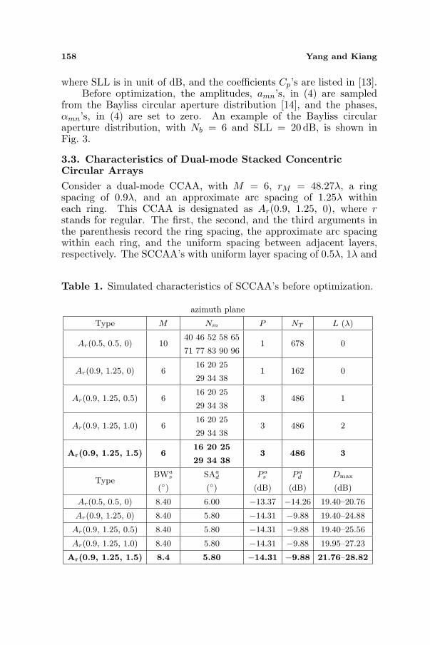
3.3. Characteristics of Dual-mode Stacked ConcentricCircular ArraysConsider a dual-mode CCAA, with M = 6, rM = 48.27λ, a ringspacing of 0.9λ, and an approximate arc spacing of 1.25λ withineach ring. This CCAA is designated as Ar(0.9, 1.25, 0), where rstands for regular. The first, the second, and the third arguments inthe parenthesis record the ring spacing, the approximate arc spacingwithin each ring, and the uniform spacing between adjacent layers,respectively. The SCCAA’s with uniform layer spacing of 0.5λ, 1λ and

Table 1. Simulated characteristics of SCCAA’s before optimization.

azimuth plane

Type M Nm P NT L (λ)

Ar(0.5, 0.5, 0) 1040 46 52 58 65

71 77 83 90 961 678 0

Ar(0.9, 1.25, 0) 616 20 25

29 34 381 162 0

Ar(0.9, 1.25, 0.5) 616 20 25

29 34 383 486 1

Ar(0.9, 1.25, 1.0) 616 20 25

29 34 383 486 2

Ar(0.9, 1.25, 1.5) 616 20 25

29 34 383 486 3

TypeBWa

s

()

SAad

()

P as

(dB)

P ad

(dB)

Dmax

(dB)

Ar(0.5, 0.5, 0) 8.40 6.00 −13.37 −14.26 19.40–20.76

Ar(0.9, 1.25, 0) 8.40 5.80 −14.31 −9.88 19.40–24.88

Ar(0.9, 1.25, 0.5) 8.40 5.80 −14.31 −9.88 19.40–25.56

Ar(0.9, 1.25, 1.0) 8.40 5.80 −14.31 −9.88 19.95–27.23

Ar(0.9, 1.25, 1.5) 8.4 5.80 −14.31 −9.88 21.76–28.82


elevation plane


Ar(0.5, 0.5, 0) 1040 46 52 58 65

71 77 83 90 961 678 0

Ar(0.9, 1.25, 0) 616 20 25

29 34 381 162 0

Ar(0.9, 1.25, 0.5) 616 20 25

29 34 383 486 1

Ar(0.9, 1.25, 1.0) 616 20 25

29 34 383 486 2

Ar(0.9, 1.25, 1.5) 616 20 25

29 34 383 486 3

TypeBWe

s

()—

P es

(dB)—

Dmax

(dB)

Ar(0.5, 0.5, 0) 44.20 – −13.37 — 19.40–20.76

Ar(0.9, 1.25, 0) 44.20 — −14.31 — 19.40–24.88

Ar(0.9, 1.25, 0.5) 44.20 — −21.26 — 19.40–25.56

Ar(0.9, 1.25, 1.0) 39.00 — −14.77 — 19.95–27.23

Ar(0.9, 1.25, 1.5) 25.60 — −16.90 — 21.76–28.82

rM = 48.27λ, P = 3 and (θ0, φ0) = (90, 0).

1.5λ, respectively, are also considered; labeled as Ar(0.9, 1.25, 0.5),Ar(0.9, 1.25, 1) and Ar(0.9, 1.25, 1.5), respectively.

The characteristics of Ar(0.9, 1.25, 0), Ar(0.9, 1.25, 0.5), Ar(0.9,1.25, 1) and Ar(0.9, 1.25, 1.5) with P = 3 and P = 5 are summarizedin Tables 1 and 2, respectively; where BWa

s () is the beamwidth ofthe sum pattern, and SAa

d () is the squint angle of the differencepattern, both in the azimuth plane; P a

s (dB) and P ad (dB) are the

maximum side-lobe level of the sum pattern and the difference pattern,respectively, in the azimuth plane. Similarly, BWe

s () and P es (dB) are

the beamwidth and the maximum side-lobe level, respectively, of thesum pattern in the elevation plane.

With the array pattern characterized in (5), the SCCAA willhave roughly the same beamwidth and side-lobe level in the azimuthplane, as those of the CCAA. In the elevation plane, however,the beamwidth and side-lobe level of the SCCAA becomes smallerthan their counterpart of the CCAA. With more layers stacked, themaximum directivity of the SCCAA is also increased [15].

160 Yang and Kiang

4. OPTIMIZATION OF STACKED CONCENTRICCIRCULAR ANTENNA ARRAYS

The design goal is to enable the same SCCAA to radiate either the sumpattern or the difference pattern, pending on the excitation signals.The side-lobe level is minimized, while the beamwidth of the sumpattern and the squint angle of the difference pattern are preserved.To achieve these requirements, the fitness function is designed as

f(ws, wd, ψs, ψd

)= fa

(ws, wd, ψs, ψd

)+ fe

(ws, wd, ψs, ψd

)(8)

where the first term and the second term on the right handside of (8) are used to specify the patterns in the azimuth planeand the elevation plane, respectively; ws = [ws1, ws2, . . . , wsN ]t,ψs = [ψs1, ψs2, . . . , ψsN ]t, wd = [wd1, wd2, . . . , wdN ]td and ψd =[ψd1, ψd2, . . . , ψdN ]t; wsn and ψsn are the amplitude and the phase,respectively, on the nth antenna element when the sum pattern isgenerated; wdn and ψdn are the amplitude and the phase, respectively,on the nth antenna element when the difference pattern is generated.The amplitude and the phase on all the elements are allowed to vary

Table 2. Simulated characteristics of SCCAA’s before optimization.

azimuth plane


Ar(0.5, 0.5, 0) 1040 46 52 58 65

71 77 83 90 961 678 0

Ar(0.9, 1.25, 0) 616 20 25

29 34 381 162 0

Ar(0.9, 1.25, 0.5) 616 20 25

29 34 385 810 2

Ar(0.9, 1.25, 1.0) 616 20 25

29 34 385 810 4

Ar(0.9, 1.25, 1.5) 616 20 25

29 34 385 810 6

TypeBWa

s

()

SAad

()

P as

(dB)

P ad

(dB)

Dmax

(dB)

Ar(0.5, 0.5, 0) 8.40 6.00 −13.37 −14.26 19.40–20.76

Ar(0.9, 1.25, 0) 8.40 5.80 −14.31 −9.88 19.40–24.88

Ar(0.9, 1.25, 0.5) 8.40 5.80 −14.31 −9.88 19.40–26.75

Ar(0.9, 1.25, 1.0) 8.40 5.80 −14.31 −9.88 22.40–29.37

Ar(0.9, 1.25, 1.5) 8.40 5.80 −14.31 −9.88 23.98–31.21


elevation plane


Ar(0.5, 0.5, 0) 1040 46 52 58 65

71 77 83 90 961 678 0

Ar(0.9, 1.25, 0) 616 20 25

29 34 381 162 0

Ar(0.9, 1.25, 0.5) 616 20 25

29 34 385 810 2

Ar(0.9, 1.25, 1.0) 616 20 25

29 34 385 810 4

Ar(0.9, 1.25, 1.5) 616 20 25

29 34 385 810 6

TypeBWe

s

()—

P es

(dB)—

Dmax

(dB)

Ar(0.5, 0.5, 0) 44.20 — −13.37 — 19.40–20.76

Ar(0.9, 1.25, 0) 44.20 — −14.31 — 19.40–24.88

Ar(0.9, 1.25, 0.5) 44.20 — −28.74 — 19.40–26.75

Ar(0.9, 1.25, 1.0) 23.00 — −14.77 — 22.40–29.37

Ar(0.9, 1.25, 1.5) 15.40 — −13.01 — 23.98–31.21

rM = 48.27λ, P = 5 and (θ0, φ0) = (90, 0).

in the range of (0, 1] and (−π, π], respectively.The first term in (8) is further decomposed as

fa(ws, wd, ψs, ψd

)

= P as

(Ωa

s

∣∣ws, ψs

)+P a

d

(Ωa

d

∣∣wd, ψd

)

+K|BWas

(ws, ψs

)−BWaso|+K

∣∣SAad

(wd, ψd

)−SAado

∣∣ (9)

where K is an empirical weighting factor. The first term and the secondterm on the right hand side of (9) are used to minimize the side-lobelevel of the sum pattern and the difference pattern, respectively; whereΩa

s and Ωad indicate the angular locations of the maximum side-lobe

level of the sum pattern and the difference pattern, respectively, in theazimuth plane. The third term on the right hand side of (9) is used toachieve the desired beamwidth, BWa

so (), of the sum pattern in theazimuth plane, measured from null to null. The last term on the righthand side of (9) is used to achieve the desired squint angle, SAa

do (),of the difference pattern in the azimuth plane.

Similarly, the second term in (8) is further decomposed as

fe(ws, wd, ψs, ψd

)= P e

s (Ωes

∣∣ws, ψs ) + K∣∣BWe

s(ws, ψs)− BWeso

∣∣ (10)

162 Yang and Kiang

where the first term and the second term on the right hand side are usedto minimize the side-lobe level and to achieve the desired beamwidth,BWe

so (), respectively, of the sum pattern in the elevation plane; Ωes

indicates the angular location of the maximum side-lobe level of thesum pattern in the elevation plane.

For comparison, the particle swarm optimization (PSO) algorithmis also applied [11]. In the PSO algorithm, a whole swarm of 20particles fly through the search space, based on the instructionsof habit, self-knowledge and social-knowledge. Both the empiricalconstants in the updating equation, C1 and C2, are set to 2 [11]. Thehabit weight, w, decreases linearly, from 0.9 to 0.4, as the iterationproceeds. The invisible boundary condition (IBC) is adopted, and the

Table 3. Parameters used in GABCA and ABCA [8].

P SN D trialmax K BWaso(

) SAado () BWe

so ()3 20 324 200 106 8.00 6.00 25.605 20 324 200 106 8.00 6.00 15.40

Table 4. Simulated characteristics of SCCAA’s after optimization.

azimuth plane


Ar(0.5, 0.5, 0) 1040 46 52 58 65

71 77 83 90 961 678 0

Ar(0.9, 1.25, 1.5) 616 20 25

29 34 383 486 3

Ag(0.9, 1.25, 1.5) 616 20 25

29 34 383 486 3

Aa(0.9, 1.25, 1.5) 616 20 25

29 34 383 486 3

Ap(0.9, 1.25, 1.5) 616 20 25

29 34 383 486 3

TypeBWa

s

()

SAad

()

P as

(dB)

P ad

(dB)

Dmax

(dB)

Ar(0.5, 0.5, 0) 8.40 6.00 −13.37 −14.26 19.40–20.76

Ar(0.9, 1.25, 1.5) 8.40 5.80 −14.31 −9.88 21.76–28.82

Ag(0.9, 1.25, 1.5) 8.40 6.00 −17.07 −15.09 21.76–28.82

Aa(0.9, 1.25, 1.5) 8.40 6.00 −14.35 −10.65 21.76–28.82

Ap(0.9, 1.25, 1.5) 8.40 6.00 −15.85 −13.48 21.76–28.82


elevation plane


Ar(0.5, 0.5, 0) 1040 46 52 58 65

71 77 83 90 961 678 0

Ar(0.9, 1.25, 1.5) 616 20 25

29 34 383 486 3

Ag(0.9, 1.25, 1.5) 616 20 25

29 34 383 486 3

Aa(0.9, 1.25, 1.5) 616 20 25

29 34 383 486 3

Ap(0.9, 1.25, 1.5) 616 20 25

29 34 383 486 3

Type BWes () — P e

s (dB) — Dmax (dB)

Ar(0.5, 0.5, 0) 44.20 — −13.37 — 19.40–20.76

Ar(0.9, 1.25, 1.5) 25.60 — −16.90 — 21.76–28.82

Ag(0.9, 1.25, 1.5) 25.60 — −24.41 — 21.76–28.82

Aa(0.9, 1.25, 1.5) 25.60 — −17.13 — 21.76–28.82

Ap(0.9, 1.25, 1.5) 25.60 — −19.51 — 21.76–28.82

rM = 48.27λ, P = 3 and (θ0, φ0) = (90, 0).

(a) (b)

Figure 4. Sum pattern of dual-mode SCCAA’s, (a) in the azimuthplane, (b) in the elevation plane, (θ0, φ0) = (90, 0), M = 6,rM = 48.27λ, P = 3, solid curve (—): Ag(0.9, 1.25, 1.5), dashedcurve (−−−): Ar(0.9, 1.25, 1.5).

164 Yang and Kiang

maximum velocity is set to 20% of the maximum coordinate in thesearch space.

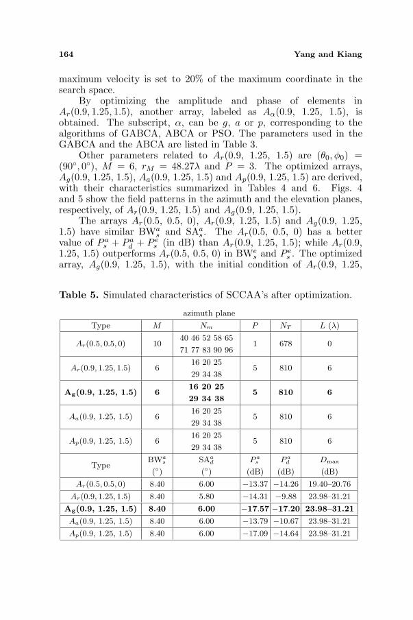
By optimizing the amplitude and phase of elements inAr(0.9, 1.25, 1.5), another array, labeled as Aα(0.9, 1.25, 1.5), isobtained. The subscript, α, can be g, a or p, corresponding to thealgorithms of GABCA, ABCA or PSO. The parameters used in theGABCA and the ABCA are listed in Table 3.

Other parameters related to Ar(0.9, 1.25, 1.5) are (θ0, φ0) =(90, 0), M = 6, rM = 48.27λ and P = 3. The optimized arrays,Ag(0.9, 1.25, 1.5), Aa(0.9, 1.25, 1.5) and Ap(0.9, 1.25, 1.5) are derived,with their characteristics summarized in Tables 4 and 6. Figs. 4and 5 show the field patterns in the azimuth and the elevation planes,respectively, of Ar(0.9, 1.25, 1.5) and Ag(0.9, 1.25, 1.5).

The arrays Ar(0.5, 0.5, 0), Ar(0.9, 1.25, 1.5) and Ag(0.9, 1.25,1.5) have similar BWa

s and SAas . The Ar(0.5, 0.5, 0) has a better

value of P as + P a

d + P es (in dB) than Ar(0.9, 1.25, 1.5); while Ar(0.9,

1.25, 1.5) outperforms Ar(0.5, 0.5, 0) in BWes and P e

s . The optimizedarray, Ag(0.9, 1.25, 1.5), with the initial condition of Ar(0.9, 1.25,

Table 5. Simulated characteristics of SCCAA’s after optimization.

azimuth plane


Ar(0.5, 0.5, 0) 1040 46 52 58 65

71 77 83 90 961 678 0

Ar(0.9, 1.25, 1.5) 616 20 25

29 34 385 810 6

Ag(0.9, 1.25, 1.5) 616 20 25

29 34 385 810 6

Aa(0.9, 1.25, 1.5) 616 20 25

29 34 385 810 6

Ap(0.9, 1.25, 1.5) 616 20 25

29 34 385 810 6

TypeBWa

s

()

SAad

()

P as

(dB)

P ad

(dB)

Dmax

(dB)

Ar(0.5, 0.5, 0) 8.40 6.00 −13.37 −14.26 19.40–20.76

Ar(0.9, 1.25, 1.5) 8.40 5.80 −14.31 −9.88 23.98–31.21

Ag(0.9, 1.25, 1.5) 8.40 6.00 −17.57 −17.20 23.98–31.21

Aa(0.9, 1.25, 1.5) 8.40 6.00 −13.79 −10.67 23.98–31.21

Ap(0.9, 1.25, 1.5) 8.40 6.00 −17.09 −14.64 23.98–31.21


elevation plane


Ar(0.5, 0.5, 0) 1040 46 52 58 65

71 77 83 90 961 678 0

Ar(0.9, 1.25, 1.5) 616 20 25

29 34 385 810 6

Ag(0.9, 1.25, 1.5) 616 20 25

29 34 385 810 6

Aa(0.9, 1.25, 1.5) 616 20 25

29 34 385 810 6

Ap(0.9, 1.25, 1.5) 616 20 25

29 34 385 810 6

TypeBWe

s

()—

P es

(dB)—

Dmax

(dB)

Ar(0.5, 0.5, 0) 44.20 — −13.37 — 19.40–20.76

Ar(0.9, 1.25, 1.5) 15.40 — −13.01 — 23.98–31.21

Ag(0.9, 1.25, 1.5) 15.40 — −13.75 — 23.98–31.21

Aa(0.9, 1.25, 1.5) 15.40 — −13.15 — 23.98–31.21

Ap(0.9, 1.25, 1.5) 15.40 — −13.21 — 23.98–31.21

rM = 48.27λ, P = 5 and (θ0, φ0) = (90, 0).

Figure 5. Difference pattern of dual-mode SCCAA’s in the azimuthplane, (θ0, φ0) = (90, 0), M = 6, rM = 48.27λ, P = 3, solid curve(—): Ag(0.9, 1.25, 1.5), dashed curve (−−−): Ar(0.9, 1.25, 1.5).

1.5), achieves a better fitness of −56.57 dB while maintaining the samebeamwidths, BWa

s , BWad and BWe

s, of Ar(0.9, 1.25, 1.5). As listed inTable 6, the GABCA achieves better fitness than the ABCA and the

166 Yang and Kiang

PSO.Next, consider Ar(0.9, 1.25, 1.5) of P = 5 layers, with (θ0, φ0) =

(90, 0), M = 6, rM = 48.27λ. The optimized arrays, Ag(0.9,1.25, 1.5), Aa(0.9, 1.25, 1.5) and Ap(0.9, 1.25, 1.5), are derived andsummarized in Tables 5 and 7. Figs. 6 and 7 show the field patternsin the azimuth plane and the elevation plane of Ar(0.9, 1.25, 1.5) andAg(0.9, 1.25, 1.5), respectively. The optimized array, Ag(0.9, 1.25, 1.5),with the initial condition of Ar(0.9, 1.25, 1.5), achieves a better fitnessof −48.52 dB while maintaining the same beamwidths, BWa

s , BWad and

(a) (b)

Figure 6. Sum pattern of dual-mode SCCAA’s, (a) in the azimuthplane, (b) in the elevation plane, (θ0, φ0) = (90, 0), M = 6,rM = 48.27λ, P = 5, solid curve (—): Ag(0.9, 1.25, 1.5), dashedcurve (−−−): Ar(0.9, 1.25, 1.5).

Figure 7. Difference pattern of dual-mode SCCAA’s in the azimuthplane, (θ0, φ0) = (90, 0), M = 6, rM = 48.27λ, P = 5, solid curve(—): Ag(0.9, 1.25, 1.5), dashed curve (−−−): Ar(0.9, 1.25, 1.5).


Table 6. Performance of GABCA, ABCA and PSO.

Algorithm P as (dB) P a

d (dB) P es (dB) fitness (dB) FI (times)

GABCA −17.07 −15.09 −24.21 −56.57 392 000ABCA −14.35 −10.65 −17.13 −42.13 611 000PSO −15.85 −13.48 −19.51 −48.84 328 000

Parameters are the same as in Table 4.

Table 7. Performance of GABCA, ABCA and PSO.

Algorithm P as (dB) P a

d (dB) P es (dB) fitness (dB) FI (times)

GABCA −17.57 −17.20 −13.75 −48.52 473 000ABCA −13.79 −10.67 −13.15 −37.61 12 000PSO −17.09 −14.64 −13.21 −44.94 523 000

Parameters are the same as in Table 5.

BWes. As listed in Table 7, Ag(0.9, 1.25, 1.5) has a better fitness than

Aa(0.9, 1.25, 1.5) and Ap(0.9, 1.25, 1.5).

5. CONCLUSION

A stacked concentric circular antenna array (SCCAA) is proposedto provide dual-mode operation in the azimuth plane and narrowerbeamwidth in the elevation plane than CCAA’s. A gbest-guidedartificial bee colony algorithm (GABCA) is applied to optimize thinnedSCCAA’s in terms of reducing the side-lobe level while maintaining thebeamwidth and the squint angle. The thinned SCCAA’s have widerelement spacings than regular SCCAA’s, with the latter as the initialcondition of optimization. The GABCA achieves better fitness thanconventional ABCA and PSO in this task.

REFERENCES

1. Rudge, A. W., K. Milne, A. D. Olver, and P. Knight, TheHandbook of Antenna Design, 2nd edition, 298–299, Inst. Engrg.Technol., 1983.

2. Panduro, M., A. L. Mendez, R. Dominguez, and G. Romero,“Design of non-uniform circular antenna arrays for side lobereduction using the method of genetic algorithms,” Int. J.Electron. Commun., Vol. 60, 713–717, 2006.

168 Yang and Kiang

3. Shihab, M., Y. Najjar, N. Dib, and M. Khodier, “Designof non-uniform circular antenna arrays using particle swarmoptimization,” J. Elect. Eng., Vol. 59, No. 4, 216–220, 2008.

4. Panduro, M. A., C. A. Brizuela, L. I. Balderas, and D. A. Acosta,“A comparison of genetic algorithms, particle swarm optimizationand the differential evolution method for the design of scannablecircular antenna arrays,” Progress In Electromagnetics ResearchB, Vol. 13, 171–186, 2009.

5. Roy, G. G., S. Das, P. Chakraborty, and P. N. Suganthan, “Designof non-uniform circular antenna arrays using a modified invasiveweed optimization algorithm,” IEEE Trans. Antennas Propagat.,Vol. 59, No. 1, 110–118, Jan. 2011.

6. Basu, B. and G. K. Mahanti, “Thinning of concentric two-ringcircular array antenna using fire fly algorithm,” Scientia Iranica,Vol. 19, No. 6, 1802–1809, Dec. 2012.

7. Yaacoub, E., M. Al-Husseini, A. Chehab, A. El Hajj, andK. Y. Kabalan, “Hybrid linear and circular antenna arrays,” Iran.J. Elec. Comput. Eng., Vol. 6, No. 1, 48–54, 2007.

8. Zhu, G. P. and S. Kwong, “Gbest-guided artificial bee colonyalgorithm for numerical function optimization,” Appl. Math.Comput., Vol. 217, No. 7, 3166–3173, Dec. 2010.

9. Basu, B. and G. K. Mahanti, “Fire fly and artificial bees colonyalgorithm for synthesis of scanned and broadside linear arrayantenna,” Progress In Electromagnetics Research B, Vol. 32, 169–190, 2011.

10. Pan, Q.-K., L. Wang, K. Mao, J.-H. Zhao, and M. Zhang, “Aneffective artificial bee colony algorithm for a real-world hybridflowshop problem in steelmaking process,” IEEE Trans. Autom.Sci. Eng., Vol. 10, No. 2, 307–322, Apr. 2013.

11. Robinson, J. and Y. Rahmat-Samii, “Particle swarm optimizationin electromagnetics,” IEEE Trans. Antennas Propagat., Vol. 52,No. 2, 397–407, Feb. 2004.

12. Milligan, T. A., Modern Antenna Design, 2nd Edition, 196–202,Wiley-Interscience, 2005.

13. Mailloux, R. J., Phased Array Antenna Handbook, 2nd Edition,132–133, Artech House, 2005.

14. Lo, Y. T. and S. W. Lee, Antenna Handbook, 13–29, van NostrandReinhold, 1988.

15. Balanis, C. A., Antenna Theory, 3rd edition, 50–52, John Wiley,2005.

TWO-DIMENSIONAL PATTERN SYNTHESIS OF STACKED …

Documents

Transcript of TWO-DIMENSIONAL PATTERN SYNTHESIS OF STACKED …