PARTPART SIX SIX - ESAC

PART SIXPART SIX

cha1873X_p06.qxd 4/12/05 11:50 AM Page 568

NUMERICALDIFFERENTIATION AND INTEGRATION

569

PT6.1 MOTIVATION

Calculus is the mathematics of change. Because engineers must continuously deal with sys-tems and processes that change, calculus is an essential tool of our profession. Standing atthe heart of calculus are the related mathematical concepts of differentiation and integration.

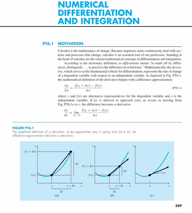
According to the dictionary definition, to differentiate means “to mark off by differ-ences; distinguish; . . . to perceive the difference in or between.” Mathematically, the deriva-tive, which serves as the fundamental vehicle for differentiation, represents the rate of changeof a dependent variable with respect to an independent variable. As depicted in Fig. PT6.1,the mathematical definition of the derivative begins with a difference approximation:

�y

�x= f(xi + �x) − f(xi )

�x(PT6.1)

where y and f(x) are alternative representatives for the dependent variable and x is theindependent variable. If �x is allowed to approach zero, as occurs in moving fromFig. PT6.1a to c, the difference becomes a derivative

dy

dx= lim

�x→0

f(xi + �x) − f(xi )

�x

FIGURE PT6.1The graphical definition of a derivative: as �x approaches zero in going from (a) to (c), thedifference approximation becomes a derivative.

f (xi)

xi xi + �x x

�x

f (xi + �x)

y y y

�y

f (xi)f ' (xi)

f (xi + �x)

xi xi + �x x

�x

(a) (b)

�y

xi x

(c)

cha1873X_p06.qxd 4/12/05 11:51 AM Page 569

570 NUMERICAL DIFFERENTIATION AND INTEGRATION

where dy/dx [which can also be designated as y′ or f ′(xi)] is the first derivative of y withrespect to x evaluated at xi. As seen in the visual depiction of Fig. PT6.1c, the derivative isthe slope of the tangent to the curve at xi.

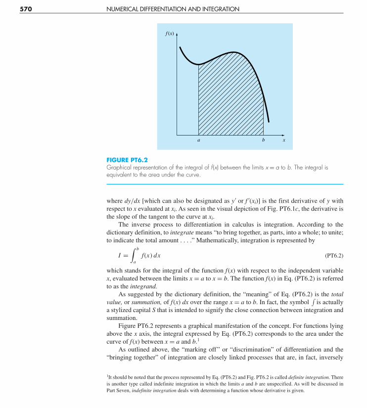
The inverse process to differentiation in calculus is integration. According to thedictionary definition, to integrate means “to bring together, as parts, into a whole; to unite;to indicate the total amount . . . .” Mathematically, integration is represented by

I =∫ b

af(x) dx (PT6.2)

which stands for the integral of the function f(x) with respect to the independent variablex, evaluated between the limits x = a to x = b. The function f(x) in Eq. (PT6.2) is referredto as the integrand.

As suggested by the dictionary definition, the “meaning” of Eq. (PT6.2) is the totalvalue, or summation, of f(x) dx over the range x = a to b. In fact, the symbol

∫is actually

a stylized capital S that is intended to signify the close connection between integration andsummation.

Figure PT6.2 represents a graphical manifestation of the concept. For functions lyingabove the x axis, the integral expressed by Eq. (PT6.2) corresponds to the area under thecurve of f(x) between x = a and b.1

As outlined above, the “marking off” or “discrimination” of differentiation and the“bringing together” of integration are closely linked processes that are, in fact, inversely

FIGURE PT6.2Graphical representation of the integral of f (x) between the limits x = a to b. The integral isequivalent to the area under the curve.

f (x)

a b x

1It should be noted that the process represented by Eq. (PT6.2) and Fig. PT6.2 is called definite integration. Thereis another type called indefinite integration in which the limits a and b are unspecified. As will be discussed inPart Seven, indefinite integration deals with determining a function whose derivative is given.

cha1873X_p06.qxd 4/12/05 11:51 AM Page 570

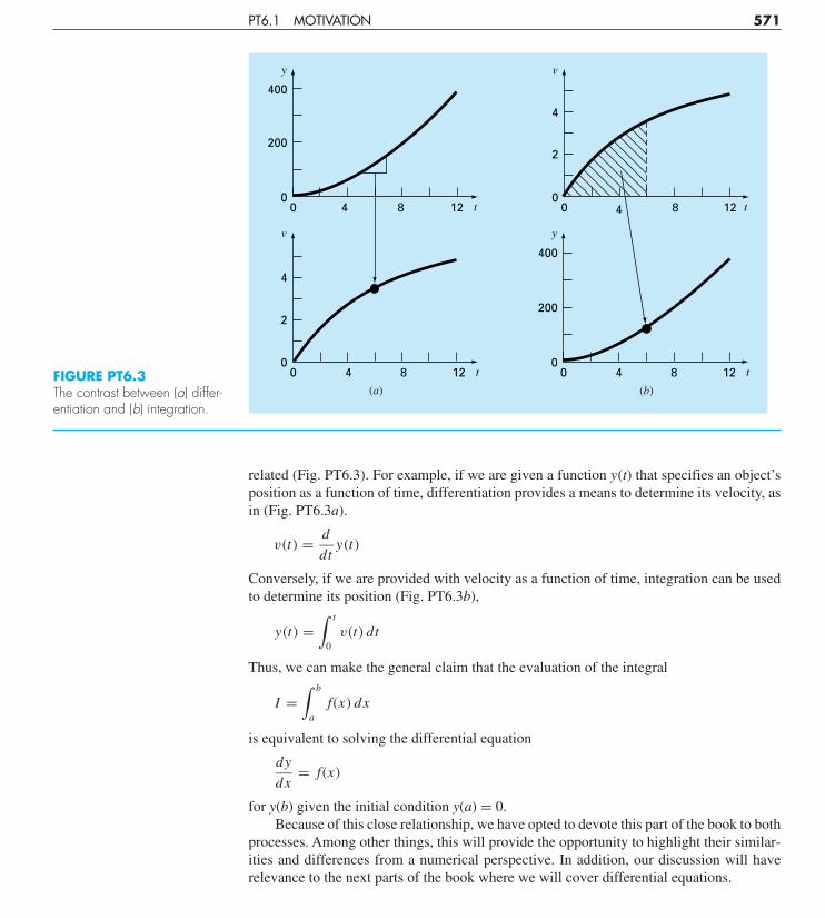
related (Fig. PT6.3). For example, if we are given a function y(t) that specifies an object’sposition as a function of time, differentiation provides a means to determine its velocity, asin (Fig. PT6.3a).

v(t) = d

dty(t)

Conversely, if we are provided with velocity as a function of time, integration can be usedto determine its position (Fig. PT6.3b),

y(t) =∫ t

0v(t) dt

Thus, we can make the general claim that the evaluation of the integral

I =∫ b

af(x) dx

is equivalent to solving the differential equation

dy

dx= f(x)

for y(b) given the initial condition y(a) = 0.Because of this close relationship, we have opted to devote this part of the book to both

processes. Among other things, this will provide the opportunity to highlight their similar-ities and differences from a numerical perspective. In addition, our discussion will haverelevance to the next parts of the book where we will cover differential equations.

PT6.1 MOTIVATION 571

FIGURE PT6.3The contrast between (a) differ-entiation and (b) integration.

y

00

200

400

8 124 t

v

00

2

4

8 124 t

v

00

2

4

8 124

(a)

t

y

00

200

400

8 124

(b)

t

cha1873X_p06.qxd 4/12/05 11:51 AM Page 571

PT6.1.1 Noncomputer Methods for Differentiation and Integration

The function to be differentiated or integrated will typically be in one of the following threeforms:

1. A simple continuous function such as a polynomial, an exponential, or a trigonometricfunction.

2. A complicated continuous function that is difficult or impossible to differentiate orintegrate directly.

3. A tabulated function where values of x and f(x) are given at a number of discretepoints, as is often the case with experimental or field data.

In the first case, the derivative or integral of a simple function may be evaluated ana-lytically using calculus. For the second case, analytical solutions are often impractical, andsometimes impossible, to obtain. In these instances, as well as in the third case of discretedata, approximate methods must be employed.

A noncomputer method for determining derivatives from data is called equal-areagraphical differentiation. In this method, the (x, y) data are tabulated and, for each inter-val, a simple divided difference �y/�x is employed to estimate the slope. Then thesevalues are plotted as a stepped curve versus x (Fig. PT6.4). Next, a smooth curve is drawnthat attempts to approximate the area under the stepped curve. That is, it is drawn so thatvisually, the positive and negative areas are balanced. The rates at given values of x canthen be read from the curve.

In the same spirit, visually oriented approaches were employed to integrate tabulateddata and complicated functions in the precomputer era. A simple intuitive approach is toplot the function on a grid (Fig. PT6.5) and count the number of boxes that approximate thearea. This number multiplied by the area of each box provides a rough estimate of the total


FIGURE PT6.4Equal-area differentiation.(a) Centered finite divideddifferences are used to estimatethe derivative for each intervalbetween the data points.(b) The derivative estimates areplotted as a bar graph. Asmooth curve is superimposedon this plot to approximate thearea under the bar graph. Thisis accomplished by drawing thecurve so that equal positive andnegative areas are balanced.(c) Values of dy/dx can then beread off the smooth curve.

x

�y�x

x

0

3

6

9

15

18

�y/�x

66.7

50

40

30

23.3

y

0

200

350

470

650

720

dy/dx

76.50

57.50

45.00

36.25

25.00

21.50

x

0

3

6

9

15

18

0 3

50

6 9

(b) (c)(a)12 15 18

cha1873X_p06.qxd 4/12/05 11:51 AM 72

area under the curve. This estimate can be refined, at the expense of additional effort, byusing a finer grid.

Another commonsense approach is to divide the area into vertical segments, or strips,with a height equal to the function value at the midpoint of each strip (Fig. PT6.6). The areaof the rectangles can then be calculated and summed to estimate the total area. In this


FIGURE PT6.5The use of a grid to approxi-mate an integral.

f (x)

a b x

FIGURE PT6.6The use of rectangles, or strips,to approximate the integral.

f (x)

a b x

cha1873X_p06.qxd 4/12/05 11:51 AM Page 573

approach, it is assumed that the value at the midpoint provides a valid approximation of theaverage height of the function for each strip. As with the grid method, refined estimates arepossible by using more (and thinner) strips to approximate the integral.

Although such simple approaches have utility for quick estimates, alternative numeri-cal techniques are available for the same purpose. Not surprisingly, the simplest of thesemethods is similar in spirit to the noncomputer techniques.

For differentiation, the most fundamental numerical techniques use finite divided dif-ferences to estimate derivatives. For data with error, an alternative approach is to fit asmooth curve to the data with a technique such as least-squares regression and then differ-entiate this curve to obtain derivative estimates.

In a similar spirit, numerical integration or quadrature methods are available to obtainintegrals. These methods, which are actually easier to implement than the grid approach, aresimilar in spirit to the strip method. That is, function heights are multiplied by strip widthsand summed to estimate the integral. However, through clever choices of weighting factors,the resulting estimate can be made more accurate than that from the simple strip method.

As in the simple strip method, numerical integration and differentiation techniques uti-lize data at discrete points. Because tabulated information is already in such a form, it isnaturally compatible with many of the numerical approaches. Although continuous func-tions are not originally in discrete form, it is usually a simple proposition to use the givenequation to generate a table of values. As depicted in Fig. PT6.7, this table can then beevaluated with a numerical method.

PT6.1.2 Numerical Differentiation and Integration in Engineering

The differentiation and integration of a function has so many engineering applications thatyou were required to take differential and integral calculus in your first year at college.Many specific examples of such applications could be given in all fields of engineering.

Differentiation is commonplace in engineering because so much of our work involvescharacterizing the changes of variables in both time and space. In fact, many of the lawsand other generalizations that figure so prominently in our work are based on the pre-dictable ways in which change manifests itself in the physical world. A prime example isNewton’s second law, which is not couched in terms of the position of an object but ratherin its change of position with respect to time.

Aside from such temporal examples, numerous laws governing the spatial behavior ofvariables are expressed in terms of derivatives. Among the most common of these are thoselaws involving potentials or gradients. For example, Fourier’s law of heat conductionquantifies the observation that heat flows from regions of high to low temperature. For theone-dimensional case, this can be expressed mathematically as

Heat flux = −k ′ dT

dx

Thus, the derivative provides a measure of the intensity of the temperature change, or gra-dient, that drives the transfer of heat. Similar laws provide workable models in many otherareas of engineering, including the modeling of fluid dynamics, mass transfer, chemical re-action kinetics, and electromagnetic flux. The ability to accurately estimate derivatives isan important facet of our capability to work effectively in these areas.


cha1873X_p06.qxd 4/12/05 11:51 AM Page 574

Just as accurate estimates of derivatives are important in engineering, the calculationof integrals is equally valuable. A number of examples relate directly to the idea of the in-tegral as the area under a curve. Figure PT6.8 depicts a few cases where integration is usedfor this purpose.

Other common applications relate to the analogy between integration and summation.For example, a common application is to determine the mean of continuous functions. InPart Five, you were introduced to the concept of the mean of n discrete data points [recallEq. (PT5.1)]:

Mean =

n∑i=1

yi

n(PT6.3)

where yi are individual measurements. The determination of the mean of discrete points isdepicted in Fig. PT6.9a.


x

f (x)

f (x)

2.599

2.414

1.945

1.993

x

0.25

0.75

1.25

1.75

00

1

2

1

Discrete points Continuousfunction

2

(c)

(b)

(a) 2 + cos (1 + x3/2)1 + 0.5 sin x

e 0.5x dx0� 2

FIGURE PT6.7Application of a numericalintegration method: (a) A com-plicated, continuous function.(b) Table of discrete values off (x) generated from the function.(c) Use of a numerical method(the strip method here) toestimate the integral on thebasis of the discrete points. Fora tabulated function, the datais already in tabular form (b);therefore, step (a) isunnecessary.

cha1873X_p06.qxd 4/12/05 11:51 AM Page 575


(a) (b) (c)

FIGURE PT6.8Examples of how integration is used to evaluate areas in engineering applications. (a) Asurveyor might need to know the area of a field bounded by a meandering stream and tworoads. (b) A water-resource engineer might need to know the cross-sectional area of a river. (c) A structural engineer might need to determine the net force due to a nonuniform windblowing against the side of a skyscraper.

FIGURE PT6.9An illustration of the mean for(a) discrete and (b) continuousdata.

y

0 4 62

Mean

3 51

ba

(a)i

y = f (x)

Mean

(b)

x

cha1873X_p06.qxd 4/12/05 11:51 AM Page 576

In contrast, suppose that y is a continuous function of an independent variable x, as de-picted in Fig. PT6.9b. For this case, there are an infinite number of values between a and b.Just as Eq. (PT6.3) can be applied to determine the mean of the discrete readings, youmight also be interested in computing the mean or average of the continuous functiony = f(x) for the interval from a to b. Integration is used for this purpose, as specified by theformula

Mean =

∫ b

af(x) dx

b − a(PT6.4)

This formula has hundreds of engineering applications. For example, it is used to calculatethe center of gravity of irregular objects in mechanical and civil engineering and to deter-mine the root-mean-square current in electrical engineering.

Integrals are also employed by engineers to evaluate the total amount or quantity of agiven physical variable. The integral may be evaluated over a line, an area, or a volume.For example, the total mass of chemical contained in a reactor is given as the product of theconcentration of chemical and the reactor volume, or

Mass = concentration × volume

where concentration has units of mass per volume. However, suppose that concentrationvaries from location to location within the reactor. In this case, it is necessary to sum theproducts of local concentrations ci and corresponding elemental volumes �Vi:

Mass =n∑

i=1

ci �Vi

where n is the number of discrete volumes. For the continuous case, where c(x, y, z) is aknown function and x, y, and z are independent variables designating position in Cartesiancoordinates, integration can be used for the same purpose:

Mass =∫ ∫ ∫

c(x, y, z) dx dy dz

or

Mass =∫ ∫

V

∫c(V ) dV

which is referred to as a volume integral. Notice the strong analogy between summationand integration.

Similar examples could be given in other fields of engineering. For example, the totalrate of energy transfer across a plane where the flux (in calories per square centimeter persecond) is a function of position is given by

Heat transfer =∫

A

∫flux dA

which is referred to as an areal integral, where A = area.


cha1873X_p06.qxd 4/12/05 11:51 AM Page 577

Similarly, for the one-dimensional case, the total mass of a variable-density rod withconstant cross-sectional area is given by

m = A∫ L

0ρ(x) dx

where m = total weight (kg), L = length of the rod (m), ρ(x) = known density (kg/m3) asa function of length x (m), and A = cross-sectional area of the rod (m2).

Finally, integrals are used to evaluate differential or rate equations. Suppose the ve-locity of a particle is a known continuous function of time v(t),

dy

dt= v(t)

The total distance y traveled by this particle over a time t is given by (Fig. PT6.3b)

y =∫ t

0v(t) dt (PT6.5)

These are just a few of the applications of differentiation and integration that you mightface regularly in the pursuit of your profession. When the functions to be analyzed are sim-ple, you will normally choose to evaluate them analytically. For example, in the fallingparachutist problem, we determined the solution for velocity as a function of time[Eq. (1.10)]. This relationship could be substituted into Eq. (PT6.5), which could then beintegrated easily to determine how far the parachutist fell over a time period t. For this case,the integral is simple to evaluate. However, it is difficult or impossible when the functionis complicated, as is typically the case in more realistic examples. In addition, the underly-ing function is often unknown and defined only by measurement at discrete points. Forboth these cases, you must have the ability to obtain approximate values for derivatives andintegrals using numerical techniques. Several such techniques will be discussed in this partof the book.

PT6.2 MATHEMATICAL BACKGROUND

In high school or during your first year of college, you were introduced to differential andintegral calculus. There you learned techniques to obtain analytical or exact derivativesand integrals.

When we differentiate a function analytically, we generate a second function that canbe used to compute the derivative for different values of the independent variable. Generalrules are available for this purpose. For example, in the case of the monomial

y = xn

the following simple rule applies (n �= 0):

dy

dx= nxn−1

which is the expression of the more general rule for

y = un


cha1873X_p06.qxd 4/12/05 11:51 AM Page 578

where u = a function of x. For this equation, the derivative is computed via

dy

dx= nun−1 du

dx

Two other useful formulas apply to the products and quotients of functions. For example,if the product of two functions of x(u and v) is represented as y = uv, then the derivativecan be computed as

dy

dx= u

dv

dx+ v

du

dx

For the division, y = u/v, the derivative can be computed as

dy

dx=

vdu

dx− u

dv

dxv2

Other useful formulas are summarized in Table PT6.1.Similar formulas are available for definite integration, which deals with determining

an integral between specified limits, as in

I =∫ b

af(x) dx (PT6.6)

According to the fundamental theorem of integral calculus, Eq. (PT6.6) is evaluated as∫ b

af(x) dx = F(x)

∣∣ba

where F(x) = the integral of f(x)—that is, any function such that F ′(x) = f(x). The nomen-clature on the right-hand side stands for

F(x)∣∣ba = F(b) − F(a) (PT6.7)

PT6.2 MATHEMATICAL BACKGROUND 579

TABLE PT6.1 Some commonly used derivatives.

�ddx� sin x = cos x �

ddx� cot x = −csc2 x

�ddx� cos x = −sin x �

ddx� sec x = sec x tan x

�ddx� tan x = sec2 x �

ddx� csc x = −csc x cot x

�ddx� ln x = �

1x� �

ddx� loga x = �

x I1n a�

�ddx� ex = ex �

ddx� ax = ax ln a

cha1873X_p06.qxd 4/12/05 11:51 AM Page 579

An example of a definite integral is

I =∫ 0.8

0(0.2 + 25x − 200x2 + 675x3 − 900x4 + 400x5) dx (PT6.8)

For this case, the function is a simple polynomial that can be integrated analytically byevaluating each term according to the rule

∫ b

axn dx = xn+1

n + 1

∣∣∣∣b

a

(PT6.9)

where n cannot equal −1. Applying this rule to each term in Eq. (PT6.8) yields

I = 0.2x + 12.5x2 − 200

3x3 + 168.75x4 − 180x5 + 400

6x6

∣∣∣∣0.8

0(PT6.10)

which can be evaluated according to Eq. (PT6.7) as I = 1.6405333. This value is equal tothe area under the original polynomial [Eq. (PT6.8)] between x = 0 and 0.8.

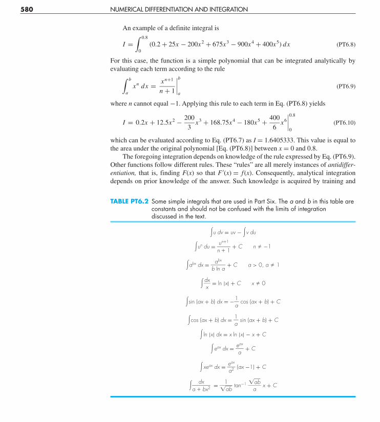
The foregoing integration depends on knowledge of the rule expressed by Eq. (PT6.9).Other functions follow different rules. These “rules” are all merely instances of antidiffer-entiation, that is, finding F(x) so that F ′(x) = f(x). Consequently, analytical integrationdepends on prior knowledge of the answer. Such knowledge is acquired by training and


TABLE PT6.2 Some simple integrals that are used in Part Six. The a and b in this table areconstants and should not be confused with the limits of integration discussed in the text.

�u dv = uv − �v du

�un du = �nu�

n+1

1� + C n � −1

�abx dx = �baIn

bx

a� + C a > 0, a � 1

��dxx� = ln |x| + C x � 0

�sin (ax + b) dx = −�1a

� cos (ax + b) + C

�cos (ax + b) dx = �1a

� sin (ax + b) + C

� ln |x| dx = x ln |x| − x + C

�eax dx = �ea

ax� + C

�xeax dx = �ea

a

2

x� (ax −1) + C

��a �

dxbx2� = �

�1ab�� tan−1 �

�aab�� x + C

cha1873X_p06.qxd 4/12/05 11:51 AM Page 580

experience. Many of the rules are summarized in handbooks and in tables of integrals. Welist some commonly encountered integrals in Table PT6.2. However, many functions ofpractical importance are too complicated to be contained in such tables. One reason whythe techniques in the present part of the book are so valuable is that they provide a meansto evaluate relationships such as Eq. (PT6.8) without knowledge of the rules.

PT6.3 ORIENTATION

Before proceeding to the numerical methods for integration, some further orientation mightbe helpful. The following is intended as an overview of the material discussed in Part Six.In addition, we have formulated some objectives to help focus your efforts when studyingthe material.

PT6.3.1 Scope and Preview

Figure PT6.10 provides an overview of Part Six. Chapter 21 is devoted to the most com-mon approaches for numerical integration—the Newton-Cotes formulas. These rela-tionships are based on replacing a complicated function or tabulated data with a simplepolynomial that is easy to integrate. Three of the most widely used Newton-Cotes formu-las are discussed in detail: the trapezoidal rule, Simpson’s 1/3 rule, and Simpson’s 3/8 rule.All these formulas are designed for cases where the data to be integrated is evenly spaced.In addition, we also include a discussion of numerical integration of unequally spaced data.This is a very important topic because many real-world applications deal with data that isin this form.

All the above material relates to closed integration, where the function values at theends of the limits of integration are known. At the end of Chap. 21, we present open inte-gration formulas, where the integration limits extend beyond the range of the known data.Although they are not commonly used for definite integration, open integration formulasare presented here because they are utilized extensively in the solution of ordinary differ-ential equations in Part Seven.

The formulations covered in Chap. 21 can be employed to analyze both tabulated dataand equations. Chapter 22 deals with two techniques that are expressly designed to inte-grate equations and functions: Romberg integration and Gauss quadrature. Computeralgorithms are provided for both of these methods. In addition, methods for evaluatingimproper integrals are discussed.

In Chap. 23, we present additional information on numerical differentiation to supple-ment the introductory material from Chap. 4. Topics include high-accuracy finite-differenceformulas, Richardson’s extrapolation, and the differentiation of unequally spaced data.The effect of errors on both numerical differentiation and integration is discussed. Finally,the chapter is concluded with a description of the application of several software packagesand libraries for integration and differentiation.

Chapter 24 demonstrates how the methods can be applied for problem solving. Aswith other parts of the book, applications are drawn from all fields of engineering.

A review section, or epilogue, is included at the end of Part Six. This review includesa discussion of trade-offs that are relevant to implementation in engineering practice. In ad-dition, important formulas are summarized. Finally, we present a short review of advanced

PT6.3 ORIENTATION 581

cha1873X_p06.qxd 4/12/05 11:51 AM Page 581

methods and alternative references that will facilitate your further studies of numericaldifferentiation and integration.

PT6.3.2 Goals and Objectives

Study Objectives. After completing Part Six, you should be able to solve many numeri-cal integration and differentiation problems and appreciate their application for engineering


PART 6Numerical

Integration andDifferentiation

CHAPTER 22Integration

ofEquations

CHAPTER 23Numerical

Differentiation

CHAPTER 24EngineeringCase Studies

EPILOGUE

PT 6.2Mathematicalbackground

PT 6.6Advancedmethods

PT 6.5Importantformulas

24.4Mechanicalengineering

24.3Electrical

engineering

24.2Civil

engineering

24.1Chemical

engineering 23.5Libraries and

packages

23.1High-accuracy

formulas

23.4Uncertain

data

23.2Richardson

extrapolation

PT 6.4Trade-offs

PT 6.3Orientation

PT 6.1Motivation

21.2Simpson's

rules

21.3Unequal

segments

21.1Trapezoidal

rule

23.3Unequal-spaced

data

21.4Open

integration

21.5Multipleintegrals

22.1Newton-Cotesfor equations

22.2Rhombergintegration

22.3Gauss

quadrature

22.4Improperintegrals

CHAPTER 21Newton-Cotes

IntegrationFormulas

FIGURE PT6.10Schematic of the organization of material in Part Six: Numerical Integration and Differentiation.

cha1873X_p06.qxd 4/12/05 11:51 AM Page 582

problem solving. You should strive to master several techniques and assess their reliability.You should understand the trade-offs involved in selecting the “best’’ method (or methods)for any particular problem. In addition to these general objectives, the specific conceptslisted in Table PT6.3 should be assimilated and mastered.

Computer Objectives. You have been provided with software and simple computer al-gorithms to implement the techniques discussed in Part Six. All have utility as learningtools.

Algorithms are provided for most of the other methods in Part Six. This informationwill allow you to expand your software library to include techniques beyond the trapezoidalrule. For example, you may find it useful from a professional viewpoint to have software toimplement numerical integration and differentiation of unequally spaced data. You mayalso want to develop your own software for Simpson’s rules, Romberg integration, andGauss quadrature, which are usually more efficient and accurate than the trapezoidal rule.

Finally, one of your most important goals should be to master several of the general-purpose software packages that are widely available. In particular, you should become adeptat using these tools to implement numerical methods for engineering problem solving.

PT6.3 ORIENTATION 583

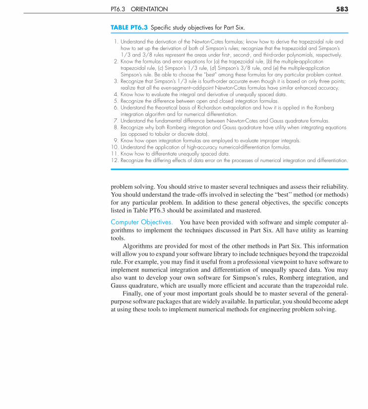
TABLE PT6.3 Specific study objectives for Part Six.

1. Understand the derivation of the Newton-Cotes formulas; know how to derive the trapezoidal rule andhow to set up the derivation of both of Simpson’s rules; recognize that the trapezoidal and Simpson’s1/3 and 3/8 rules represent the areas under first-, second-, and third-order polynomials, respectively.

2. Know the formulas and error equations for (a) the trapezoidal rule, (b) the multiple-applicationtrapezoidal rule, (c) Simpson’s 1/3 rule, (d ) Simpson’s 3/8 rule, and (e) the multiple-applicationSimpson’s rule. Be able to choose the “best” among these formulas for any particular problem context.

3. Recognize that Simpson’s 1/3 rule is fourth-order accurate even though it is based on only three points;realize that all the even-segment–odd-point Newton-Cotes formulas have similar enhanced accuracy.

4. Know how to evaluate the integral and derivative of unequally spaced data.5. Recognize the difference between open and closed integration formulas.6. Understand the theoretical basis of Richardson extrapolation and how it is applied in the Romberg

integration algorithm and for numerical differentiation.7. Understand the fundamental difference between Newton-Cotes and Gauss quadrature formulas.8. Recognize why both Romberg integration and Gauss quadrature have utility when integrating equations

(as opposed to tabular or discrete data).9. Know how open integration formulas are employed to evaluate improper integrals.

10. Understand the application of high-accuracy numerical-differentiation formulas.11. Know how to differentiate unequally spaced data.12. Recognize the differing effects of data error on the processes of numerical integration and differentiation.

cha1873X_p06.qxd 4/12/05 11:51 AM Page 583

PARTPART SIX SIX - ESAC

Documents

Transcript of PARTPART SIX SIX - ESAC