1

Particle Image Velocimetry using Feature Tracking and Delaunay tessellation

M. Miozzi*

Università di Roma “La Sapienza” Dipartimento Idraulica, Trasporti e Strade Via Eudossiana, 18 - 00184 Rome; Italy

E-Mail: m.miozzi@tin.it

ABSTRACT

This work presents YATS (Yet Another Tracking Software), an application of Feature Tracking (FT) and Computational Geometry techniques to the measure of fluid flows. From a general point of view, FT can be considered as a correlation based method, working on interrogation windows, for tracking features inside high, medium and low seeded images. FT defines its best correlation measure as the minimum of the Sum of Squared Differences (SSD) of intensity values of pixels between the interrogation windows in two consecutive frames. The implemented algorithm is able to extract interrogation window displacement and deformations from frame to frame adopting, in consecutive steps, two different models of motion for the window itself: a pure translational model, in which a rigid motion hypothesis is adopted, and an affine one, in which first order window deformation parameters are taken into account, allowing the interrogation spot to be translated, rotated, scaled and sheared. For small motions, a linearization of the image intensity leads to solve the SSD minimization problem in a Newton-Raphson style. Velocity computation is performed where the solution of FT linear system exists, i.e. where image intensity gradients are not null both in x and y directions (features). Velocity and velocity gradients are obtained, in a lagrangian fashion, along the trajectory of each feature. As a result, high-density-in-space lagrangian measurements are gained, in terms of fluid velocity and velocity spatial derivatives. Lagrangian information is then embedded into a Delaunay tessellation, which is uniquely defined by the spatial relative positions of the features tracked from time t to t+1: the Eulerian fields of velocity and velocity spatial derivatives are obtained by applying the Natural Neighbours (NN) interpolation algorithm on the Delaunay tessellation itself, for an arbitrary sized grid. In NN method the support for data interpolation is not defined by the same measure in all directions, but is allowed to be non isotropic: support size in r direction is not given by an L2 metric but is a consequence of the geometric construct that defines the region of interaction between the features.

Results obtained for two kinds of synthetic images are shown: array of vortices and Std. set of the Visualization Society of Japan. The accuracy of the method is highlighted both in Lagrangian and Eulerian framework.

0 50 100 150 200 250

0

50

100

150

200

250

Pixel

Pix

el

a)

Pixels

Pix

els

50 100 150 200 250

50

100

150

200

250

-0.6 0.6

b)

Fig. 1: Synthetic images of an array of vortexes with 15.5 pixel core. Lagrangian velocity field (a) (vectors are out of scale for clarity) and Lagrangian vorticity field (b) after FT analysis. Vorticity is plotted on the support of a Delaunay tessellation that uses the feature positions in a) as reference nodes and fills each triangle with a demonstrative vorticity value obtained as linear interpolation of measured data at its vertexes.

*Correspondence address: Via Elio Stilone 20, 00174 – Rome - Italy

2

INTRODUCTION

Among optical methods for scientific and industrial non-invasive measure of the velocity inside a flow, Particle Image Velocimetry plays a major rule because of its ability to extract the whole eulerian velocity field on a regular grid. The experimental seeding condition of the flow defines two extreme limits inside the class of PIV techniques: the low-particle-density mode (referred as Particle Tracking Velocimetry, PTV) and the high-particle-density mode (referred as Particle Image Velocimetry, PIV). Both methods inherently measure the Lagrangian velocity of particles (Adrian, 1991), but they strongly differ in algorithmic and results structure.

Classical PTV low density image analysis methods (Lewis et al., 1987; Kobayashi et al, 1989 among others) look for centroid position of seeding particles in at least three consecutive frames, adopting centroid-matching strategies based on maximum displacement, maximum acceleration, preferential direction etc. Those PTV techniques are not applicable to calculating the velocity in flows subject to strong deformation, because they deal with fluid motion mainly due to translation: additional constrains are required to solve the fluid flow. Tracking methods that use two frames analysis have been developed too, based on the investigation of the highest match probability built on the accumulated number of matches obtained by iterative calculations (Baek and Lee, 1996), on the spring model method (Okamoto et al., 1995), on the tracking of triangle elements of a Delaunay tessellation (Song et al., 1999) and on the use of the velocity gradient tensor (Ishikawa et al., 2000). Among PTV algorithms that use a correlation function as a tracking criterion, here the work by Gui and Merzkirch (2000) is reminded. This method uses the Minimum Quadratic Difference (MQD) algorithm, a method that looks quite similar to the minimization of the Sum of Squared Difference (SSD).

The basic idea of PIV high-density image analysis methods is the identification of similar particle patterns in two subsequent PIV images, via the application of a matching criterion. The classical PIV operates directly on intensity values of couples of subsequent images. The analysed area is subdivided in many interrogation windows, supported on a regular grid, with a certain degree of overlapping: velocity vectors of the eulerian field are obtained finding the displacement between the investigated region and its “most similar region” at next time. The matching measure is chosen as the inner product between the interrogation windows. The position of the centroid of the sharpest peak in cross-correlation function is a measure of the average displacement taken over the investigated region. The most important limits in conventional cross-correlation PIV algorithms can be summarized in two categories: limits in the accuracy, due to the assumption that velocity gradients inside the interrogation window are negligible and limits in velocity dynamic range, due to the conflict between the interrogation window size and the in-plane displacement that causes loss-of-pairs (Adrian 1991).

In order to avoid these problems, different approaches have been proposed in literature: Huang et al. (1993) and Jambunathan et al. (1995) first proposed image deformation based techniques (see Scarano, 2002 for a review). Advanced PIV methods introduced a local field correction function in order to allow interrogation window deformation (Nogeira et al., 1999) and the use of iterative multigrid analysis in order to reduce the size of the interrogation window (Scarano and Riethmuller, 2001 among the others).

Other two non classical PIV methods are reminded here, because of their affinity with the technique proposed by the author: the Correlation Image Velocimetry (CIV), by Tokumaru and Dimotakis (1995), that minimizes a Lagrangian function of the scalar image intensity field, and the Direct Measurement of Vorticity (DMV), by Ruan et al. (2001), that performs the direct evaluation of the vorticity from the analysis of the image flow rotation.

The YATS method here proposed relies on Feature Tracking (FT), a correlation based tracking procedure, and on the Natural Neighbours interpolation (NN), which is applied to obtain data on a regular grid. The FT, a well-known image alignment algorithm, can be considered as a Particle Image Velocimetry technique based on a distance measure minimization problem (Lukas and Kanade, 1981). This method defines the best matching measure between windows in two consecutive frames as the minimum of the Sum of Squared Differences (SSD) between intensity values of pixels in two interrogation windows at time t and t+1. The warp W that maps pixels from their position x(x, y) in the image at time t to their position in the image at time t+1 is chosen as a priori hypothesis about the model of motion of the flow inside the image. For small displacements, a linearization of the image intensity leads to a Newton-Raphson style minimization (Tomasi and Kanade, 1991, Shi and Tomasi, 1994). The problem is solved, using a pyramidal representation of the images (Burt and Adelson, 1983), in two consecutive steps: in the first step the window displacement is obtained using a pure translational warp as motion model; in the second step the use of an affine warp, that allows translation, rotation,

scale and shear of the interrogation spot, permits the direct, lagrangian measure of the velocity gradients j

i

xu

∂∂

and the

refinement of the displacement estimation.

The uniqueness of FT in PIV systems framework concerns the selection of the investigated spots: SSD minimization system is solved only in the neighbourhood of points, called “good features to track”, where preliminary analysis of texture patterns has confirmed the existence of a numerically well-defined solution (Tomasi and Kanade, 1991, Shi and Tomasi, 1994). In other words, this method supplies a quantitative measure of the trackability of a feature inside the

3

image: this measure relies on the solvability condition of the tracking algorithm and guarantees the existence and the precision of the result.

In order to extract eulerian velocity fields from FT results and with the general aim of retaining and maximizing the information content of unstructured lagrangian data, a Delaunay triangulation (Voronoi 1908, Delaunay 1934) is built using tracked features positions as reference nodes and assigning to each node the corresponding measured quantities (velocities and their spatial derivatives). Natural Neighbour (NN) approach (Watson 1981, Sambridge et al. 1995) is then applied to interpolate sparse data on a regular grid.

The NN interpolation is a local procedure that completely differs from the classical surface approximation schemes, in which weight function is usually isotropic (circular in 2-D), non-negative within a circle of some fixed radius, and monotonically decreasing with distance from some point x. All those approaches impose that nodes that are closer to x give a larger weight at x than those placed at greatest distance. NN method is based on the idea that the NN coordinate of a point x is not defined by the same measure in all directions, but it is a consequence of the geometric construct that defines the region of interaction between the features. Grids with different cell size that share a set of nodes will show the same data in the shared nodes.

Two types of images are analysed: the first type underlies analytical velocity fields (Nogeira et al., 2002); the second type is the Visualization Society of Japan Std. set of images (Okamoto et al, 2000). The former type permits the direct comparison of lagrangian results of FT tracking and the estimation of the error introduced by the gridding technique; the latter type offers a representation of FT performances in various conditions of flow seeding, particle dimension and particle displacement, in an eulerian framework.

The paper is organized as follows: in Chapter 1 a background of the FT algorithm is reported. The Chapter 2 reports a description of the NN interpolation and in Chapter 3 results for synthetic data are shown.

1 BACKGROUND OF FEATURE TRACKING

Let’s consider a sequence of images recording the motion of a particle in a 3D fluid flow. If I(x, y) is the matrix containing the intensity values inside the image, and u = [u(x, y) v(x, y)] the 2D motion field projection on the CCD image plane, the equation governing I variations can be written as:

tDID

yI

vxI

utI

=∂∂

+∂∂

+∂∂

Eq. 1-1

under the condition of small displacements between images at different times.

Eq. 1-1 represents the substantial derivative of luminosity inside the image: if we consider all surfaces inside the image to have Lambertian characters (their luminosity values do not depend on the point of view of the observer) and the illumination source to give almost constant level of light, the right member of Eq. 1-1 can be considered as zero; in this way the continuity equation for the optical flow, also called Brightness Constancy Constrain (BBC), is obtained:

0=∇+=∂∂

+∂∂

+∂∂ T

t uIIvyI

uxI

tI

, Eq. 1-2

where:

( ) ( ) ( )

∂

∂∂

∂=∇

ytxI

xtxI

txI,,

, and tI

I t ∂∂

= .

The basis of the measurement principle is the comparison of two images obtained in a finite time interval, then the intermediate transport process along the path line of the particle has not to be considered. Eq. 1-1 represents the lagrangian derivative of luminance function, taking in account all non-linear effects in luminosity changes: it can be used as a cost function evaluating the change in image luminosity levels due to external factors. Naming C the path of the particle from the first to the second image, a cost function ε can be expressed as:

22

=

∂∂

+∂∂

+∂∂

= ∫∫CC

sdtDID

sdyI

vxI

utI

ε

Eq. 1-3

When the terminal points of path line are expressed as A and B and I and J are the images at time t and t+1, the cost function can be obtained simply using the luminance values IA, JB as follows:

[ ] 2AB IJ −=ε Eq. 1-4

4

Eq. 1-4 is computed in a single point; it only provides one equation for the motion unknowns. Eq. 1-4 is able to provide enough constrains on u only when the same equation is evaluated at each point in a region R(x) surrounding a particle: the cost function takes the name of SSD and the over determined linear system is solved via a Newton-Raphson style minimization algorithm.

1.1 Interrogation window warping

Naming warp W(x, p) the operator that maps pixels x from frame I at time t to frame J at time t+1, the goal of the FT algorithm is to minimize the SSD:

[ ] [ ]∑ ∑ −=−+=R R

xIpxWJtxItxJSSD 22 )()),(())(())1(( .

This system is solved via a minimization procedure: if we suppose that initial value p0 of p is known, the problem starts from p0 and is iteratively solved for increments of the parameters ∆p; the following equation is (approximatively) minimized:

min

2min ))()),(((∑ −∆+=

R

xIppxWJSSD Eq. 1-5

in respect to ∆p, and then updated with p ? p + ∆p (Baker and Matthews, 2004). Those two steps are repeated until the norm || ∆p|| 2 is lower than a prefixed threshold.

1.2 FT algorithm

The non-linear Eq. 1-5 can be linearized by means of first order Taylor expansion of J(W(x, p+ ∆p)):

min

2

min ))()),((∑

−∆

∂∂

∇+≈R

xIpp

WIpxWJSSD Eq. 1-6

The term p

W∂∂

represents the Jacobian of the warp W: considering [ ]YX WWW = , then

∂∂

∂∂

∂∂

∂∂

∂∂

∂∂

=∂

∂

n

YYY

n

XXX

pW

pW

pW

pW

pW

pW

pW

...

...

21

21 .

The parameters number n can be arbitrarily large and the warp W can be arbitrarily complex (Baker and Matthews, 2004): nevertheless, numerical instabilities rising are strictly related with the parameters number n.

The minimization problem in Eq. 1-6 is a least-square problem and admits a closed form solution: deriving Eq. 1-6 in respect to ∆p yields to:

( ) 0)(),( =

−∆

∂∂

∇+

∂∂

∇∑R

T

xIpp

WIpxWJ

pW

I ,

from which the linear system for parameters increment is obtained:

bGp 1−=∆ Eq. 1-7

where:

∑

∂∂

∇

∂∂

∇=R

T

pW

Ip

WIG and [ ] ∑∑

∂∂

∇−=−

∂∂

∇=R

tR

Ip

WIpxWJxI

pW

Ib )),(()(

with ( )( ) ( )xIpxWJtI

I t −=∂∂

= , .

5

Eq. 1-7 is iteratively solved until threshp <∆2

or the number of iterations exceeded a maximum value: in the

former case, the feature is validated; in the latter case the feature is rejected.

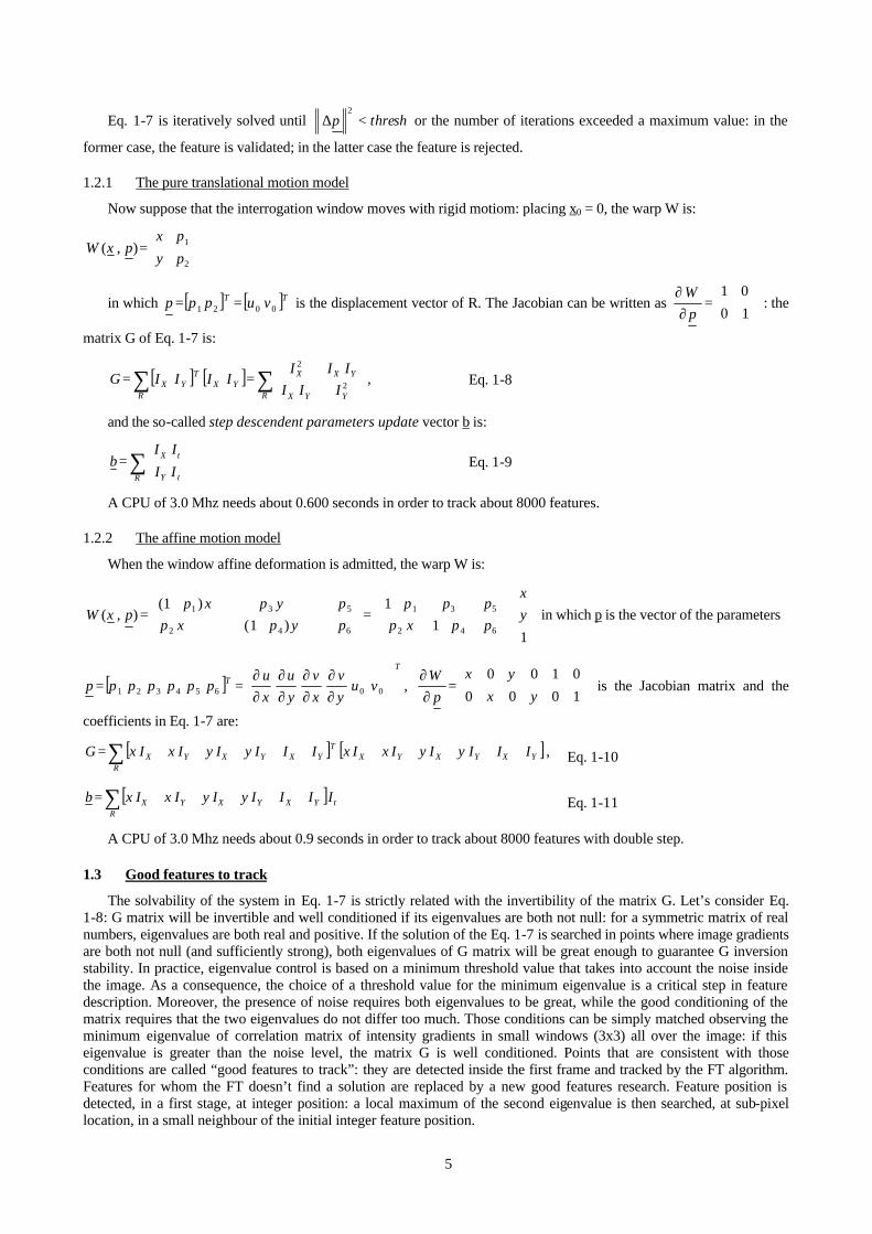
1.2.1 The pure translational motion model

Now suppose that the interrogation window moves with rigid motiom: placing x0 = 0, the warp W is:

++

=2

1),(pypx

pxW

in which [ ] [ ]TT vuppp 0021 == is the displacement vector of R. The Jacobian can be written as

=

∂∂

1001

pW

: the

matrix G of Eq. 1-7 is:

[ ] [ ]∑ ∑

==

R R YYX

YXXYX

TYX III

IIIIIIIG 2

2

, Eq. 1-8

and the so-called step descendent parameters update vector b is:

∑

=

R tY

tX

IIII

b

Eq. 1-9

A CPU of 3.0 Mhz needs about 0.600 seconds in order to track about 8000 features.

1.2.2 The affine motion model

When the window affine deformation is admitted, the warp W is:

⋅

+

+=

++++++

=

11

1)1(

)1(),(

642

531

642

531 yx

ppxpppp

pypxppypxp

pxW in which p is the vector of the parameters

[ ]T

T vuyv

xv

yu

xu

ppppppp

∂∂

∂∂

∂∂

∂∂

== 00654321 ,

=

∂∂

1001

0000yx

yxp

W is the Jacobian matrix and the

coefficients in Eq. 1-7 are:

[ ] [ ]∑=R

YXYXYXT

YXYXYX IIIyIyIxIxIIIyIyIxIxG , Eq. 1-10

[ ]∑=R

tYXYXYX IIIIyIyIxIxb Eq. 1-11

A CPU of 3.0 Mhz needs about 0.9 seconds in order to track about 8000 features with double step.

1.3 Good features to track

The solvability of the system in Eq. 1-7 is strictly related with the invertibility of the matrix G. Let’s consider Eq. 1-8: G matrix will be invertible and well conditioned if its eigenvalues are both not null: for a symmetric matrix of real numbers, eigenvalues are both real and positive. If the solution of the Eq. 1-7 is searched in points where image gradients are both not null (and sufficiently strong), both eigenvalues of G matrix will be great enough to guarantee G inversion stability. In practice, eigenvalue control is based on a minimum threshold value that takes into account the noise inside the image. As a consequence, the choice of a threshold value for the minimum eigenvalue is a critical step in feature description. Moreover, the presence of noise requires both eigenvalues to be great, while the good conditioning of the matrix requires that the two eigenvalues do not differ too much. Those conditions can be simply matched observing the minimum eigenvalue of correlation matrix of intensity gradients in small windows (3x3) all over the image: if this eigenvalue is greater than the noise level, the matrix G is well conditioned. Points that are consistent with those conditions are called “good features to track”: they are detected inside the first frame and tracked by the FT algorithm. Features for whom the FT doesn’t find a solution are replaced by a new good features research. Feature position is detected, in a first stage, at integer position: a local maximum of the second eigenvalue is then searched, at sub-pixel location, in a small neighbour of the initial integer feature position.

6

Note that the concept of good features to track has been introduced as a requirement of the tracking algorithm: “a feature is good if it can be tracked well” (Tomasi and Kanade, 1991). The uniqueness of FT concerns the suggestion of a quantitative measure of the quality of the tracking results, the G-1 matrix, providing that it is evaluated in points (the good features set) where the solution of tracking exists and is well conditioned.

1.4 The pyramidal double-step procedure

In YATS implementation of FT, the described algorithms are embedded in a pyramidal representation of frames at time t and t+1. A pyramidal representation with L levels of an image is built placing the original image at level 0; all other levels are obtained convolving the image at level l-1 with a 5x5 gaussian window, then selecting odd rows and columns and placing the result at level l. In this way the ratio between interrogation window and image size at level l is improved of 2l (l=0..L). The Lukas-Kanade process that starts at level L (usually not greater than 3) works with small particle displacements, as required from theory, and the in- plane loss of pair problem is greatly reduced. Results of tracking are propagated, as initial seeds, at level L-1 and so on, until level 0 is reached. Pyramidal approach doesn’t differ from multigrid PIV approach. It’s advantages are the noise reduction in images at level l>0 (due to the convolution with a gaussian window) and a constant complexity of the code: the interrogation window has always the same dimension at each level l of the pyramid.

Operatively, YATS method performs the tracking following two steps: after detection of good features to track at level 0 and their propagation at the higher pyramid level, each feature is tracked using the translational motion model; if the feature has been tracked at level l, it is then propagated at level l-1, until level 0 is reached. After this step, the same feature is tracked by means of the affine motion model that takes, as seeding initial condition, the displacement found after translational tracking. In this way, the numerical instabilities that rises when evaluating displacement derivatives in affine motion model are negletted from the use of good initial seeds obtained from the pure translational motion model.

Fig. 2: interrogation window before and after gaussian convolution and photometric normalization

440 442 444 446 448 450205

206

207

208

209

210

211

212

213

214

215

Pixel

Pix

el

Fig. 4: a zoom of the vortex core in Fig. 3.

410 420 430 440 450 460 470 480

185

190

195

200

205

210

215

220

225

230

235

Pixel

Pix

el

Fig. 3: displacement and deformation of tracked interrogation spots over an experimental sequence of 6 frames. The first window of the sequence (blue dashed line) is warped iteratively to show time evolution of window deformation (last window in red). Displacement in green. Spot size has been reduced from 11 px to 4 px.

In applying the described procedure, interrogation windows intensity values are convolved with a gaussian window of the same size, with m⋅= 5.0σ , where m is the half side of the interrogation window. Moreover, photometric normalization on DN vector I of image intensity values is adopted (i.e. the original values are transformed in a zero mean and unitary standard deviation set, see Fig. 2) and robust outliers detection is performed (Tommasini et al., 1998), in order to monitor the quality of the tracked features.

The monitoring is founded on the observation of the residuals when comparing good features surrounding (almost identical) windows from a frame to the next one. If we assume that the intensity of each pixel in the current frame window is the same of that in the previous frame, plus a gaussian additive noise, the square of a gaussian random variable has a chi-square distribution. The sum of n chi square random variables with one degree of freedom is distributed as a chi-square with n degrees of freedom. Therefore, the residual computed over a NxN window is

7

distributed as a chi-square with N2 degrees of freedom. As the number of degree of freedom increases, the chi-square distribution approaches a gaussian (distributions with more than 30 degrees of freedom); therefore, since the interrogation window dimension, for each feature, is at least 7x7 pixels, it is possible to safely assume a gaussian distribution for the residuals of a good feature. When a tracked feature is a bad feature, its residual is not a sample from a gaussian: it is an outlier. From this point of view, bad feature detection can be approached using a simple but effective model-free rejection rule, X84, which achieves robustness by employing median and median deviation instead of the usual mean and standard deviation. This rule prescribes to reject values that are more than k times the Median Absolute Deviations (MADs) away from the median:

−= j

ji

imedmedMAD εε Eq. 1-12

where εi,j are the residuals in points i and j of the interrogation spot. In practice, a value of k=5.2 has been used.

An example of the final result of the tracking procedure is sketched in Fig. 3 and Fig. 4, in which displacement and deformation are shown for a set of interrogation windows during a 6 frames sequence of real images. The deformation is iteratively applied, in order to show the continuity of the tracking during the sequence analysis.

2 NATURAL NEIGHBOURS INTERPOLATION

In order to maximize the spatially unstructured velocity data information contain, Voronoi tessellation and its dual, Delaunay triangulation (Voronoi 1908, Delaunay 1934), have been chosen as tools for obtaining regular pictures of the flow.

In the following sections, the term node is referred to a feature, while the term point is referred to an element of the 2-D plane. Consider a set of N distinct nodes N={n1…nm}: the Voronoi diagram (first order diagram) of the set N is a subdivision of the plane into regions TI (closed and convex, or unbounded) associated with a node nI, such that any point in TI is closer to nI than to any other node NnJ ∈ . For all the nodes inside the convex hull, Voronoi polygons are closed

and convex, while the polygons associated with nodes on the boundary of the convex hull are unbounded.

The Delaunay triangulation is constructed by connecting the nodes where Voronoi cells have common boundaries. The duality between the two geometric structures implies that there is a Delaunay edge between two nodes in the plane if and only if their Voronoi cells share a common edge. The Delaunay triangulation is completely defined if the Voronoi decomposition is known, and vice-versa.

Delaunay triangles are of interest because of their useful properties. They represent the “best looking” set of triangles, in the sense that the minimum internal angle of each triangle is maximized (Lawson, 1977). Another important property of the triangulation is the “empty circumcircle” criterion (Lawson, 1977): if DT (ni, nj, nk) is any Delaunay triangle of the data set N, then the circumcircle of DT contains no other nodes of N. An example of Delaunay tessellation is shown in Fig. 1 b).

2.1 Natural neighbours interpolation method

The NNs of a node Nn ∈ are those nodes in the neighbouring Voronoi cells or, equivalently, those to which the node is connected by the sides of Delaunay triangle. NNs concept can be extended to any point P(x, y) of the plane: in this case they can be identified as those points to which P(x, y) would be connected if it was added to the Delaunay triangulation. In other words, NN of P(x, y) are the points whose triangulation relationships were modified by the new point insertion. An operative consequence of this consideration is that a node Nn ∈ is a NN for the point P(x, y) if the circumcircle of one or more triangles having n as vertex contains the point P(x, y).

1 2

GP

3

4

5

Fig. 5: circumtriangles of grid point GP.

5

4

3

2

1

GP

A5

A4

A1 A2

A3

Fig. 6: II° order Voronoi polygon for the point GP of Fig. 5.

8

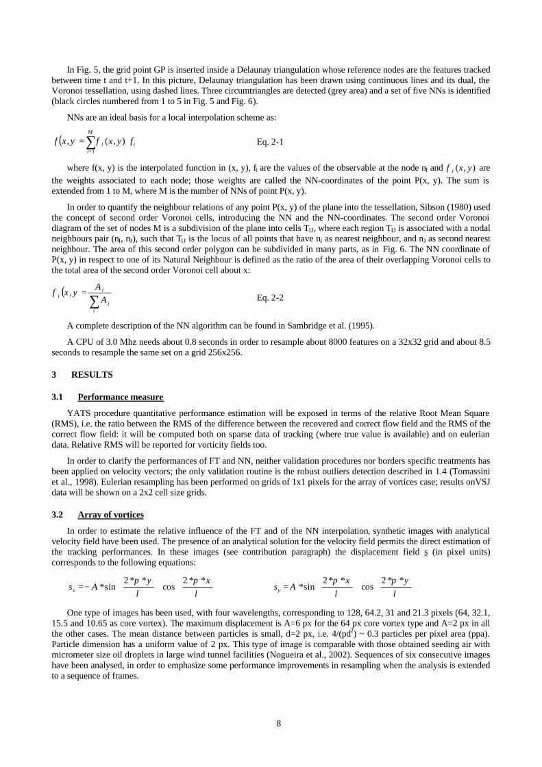
In Fig. 5, the grid point GP is inserted inside a Delaunay triangulation whose reference nodes are the features tracked between time t and t+1. In this picture, Delaunay triangulation has been drawn using continuous lines and its dual, the Voronoi tessellation, using dashed lines. Three circumtriangles are detected (grey area) and a set of five NNs is identified (black circles numbered from 1 to 5 in Fig. 5 and Fig. 6).

NNs are an ideal basis for a local interpolation scheme as:

( ) ∑=

⋅=M

iii fyxyxf

1

),(, φ Eq. 2-1

where f(x, y) is the interpolated function in (x, y), fi are the values of the observable at the node nI and ),( yxiφ are the weights associated to each node; those weights are called the NN-coordinates of the point P(x, y). The sum is extended from 1 to M, where M is the number of NNs of point P(x, y).

In order to quantify the neighbour relations of any point P(x, y) of the plane into the tessellation, Sibson (1980) used the concept of second order Voronoi cells, introducing the NN and the NN-coordinates. The second order Voronoi diagram of the set of nodes M is a subdivision of the plane into cells TIJ, where each region TIJ is associated with a nodal neighbours pair (nI, nJ), such that TIJ is the locus of all points that have nI as nearest neighbour, and nJ as second nearest neighbour. The area of this second order polygon can be subdivided in many parts, as in Fig. 6. The NN coordinate of P(x, y) in respect to one of its Natural Neighbour is defined as the ratio of the area of their overlapping Voronoi cells to the total area of the second order Voronoi cell about x:

( )∑

=

ii

ii A

Ayx ,φ

Eq. 2-2

A complete description of the NN algorithm can be found in Sambridge et al. (1995).

A CPU of 3.0 Mhz needs about 0.8 seconds in order to resample about 8000 features on a 32x32 grid and about 8.5 seconds to resample the same set on a grid 256x256.

3 RESULTS

3.1 Performance measure

YATS procedure quantitative performance estimation will be exposed in terms of the relative Root Mean Square (RMS), i.e. the ratio between the RMS of the difference between the recovered and correct flow field and the RMS of the correct flow field: it will be computed both on sparse data of tracking (where true value is available) and on eulerian data. Relative RMS will be reported for vorticity fields too.

In order to clarify the performances of FT and NN, neither validation procedures nor borders specific treatments has been applied on velocity vectors; the only validation routine is the robust outliers detection described in 1.4 (Tomassini et al., 1998). Eulerian resampling has been performed on grids of 1x1 pixels for the array of vortices case; results onVSJ data will be shown on a 2x2 cell size grids.

3.2 Array of vortices

In order to estimate the relative influence of the FT and of the NN interpolation, synthetic images with analytical velocity field have been used. The presence of an analytical solution for the velocity field permits the direct estimation of the tracking performances. In these images (see contribution paragraph) the displacement field s (in pixel units) corresponds to the following equations:

⋅

−=

λπ

λπ xy

Asx**2

cos**2

sin*

⋅

=

λπ

λπ yx

Asy**2

cos**2

sin*

One type of images has been used, with four wavelengths, corresponding to 128, 64.2, 31 and 21.3 pixels (64, 32.1, 15.5 and 10.65 as core vortex). The maximum displacement is A=6 px for the 64 px core vortex type and A=2 px in all the other cases. The mean distance between particles is small, d=2 px, i.e. 4/(pd2) ~ 0.3 particles per pixel area (ppa). Particle dimension has a uniform value of 2 px. This type of image is comparable with those obtained seeding air with micrometer size oil droplets in large wind tunnel facilities (Nogueira et al., 2002). Sequences of six consecutive images have been analysed, in order to emphasize some performance improvements in resampling when the analysis is extended to a sequence of frames.

9

3.2.1 Measure of velocity and vorticity

The FT algorithm starts its chain of analysis detecting the features that are good to track: this means that image pixels are investigated in order to evaluate the minimum eigenvalue of intensity gradients correlation matrix.

The image is visited in each pixel and, if a minimum threshold condition is verified, a local maxima algorithm looks for better feature position at sub-pixel precision. After this phase, a minimum distance condition is applied to the good features set: higher minimum eigenvalue features are chosen. At this time, the starting features position is heavily conditioned from the integer position of the pixels inside the image and from the minimum distance condition. This situation is typical when we analyse couples of images, like in PIV classical cross-correlation camera images. In the analysis of sequences of frames, the features tracked from time t to time t+1 are all included in the new set of good features for the tracking from t+1 to t+2: a new search of other good features starts and, in respect of the minimum distance condition, other features are added in places where tracked features density is small. Fig. 7shows the number of tracked features for four six-frames sequence.

Fig. 7: evolution of the feature number during tracking.

Fig. 8: relative rms vs time of the velocity field after tracking

Fig. 9: relative rms vs time after resampling

During the track, the quality of the tracking remains almost the same for each couple of frames, but the number of tracked features greatly improves: in this way, a greater number of reference points are furnished to the resampling algorithm, and a certain improvement of the resulting eulerian velocity field is recorded. This result is shown in Fig. 8 and Fig. 9: relative rms of lagrangian data shows almost constant values, while relative rms of eulerian data decreases as the number of tracked features improve.

The same result has been obtained for the vorticity data: Fig. 10 shows the evolution of relative rms value for the sparse vorticity field obtained after tracking, Fig. 11 shows the relative rms of vorticity data after resampling on a regular grid. A direct comparison of performance evolution after resampling at time t=1 and at time t=5 is reported in Fig. 12 both for velocity (V) and vorticity (W).

Fig. 10: relative rms vs time of the vorticity field after tracking

Fig. 11: relative rms vs time of vorticity field after resampling

Fig. 12: comparison of the relative rms after resampling at time t=1 and t=5

A visual sketch of the general consistency of the measured quantities is drawn in pictures from Fig. 13 to Fig. 18, in which true data are plotted using dots and measured data with a continuous line: horizontal velocity and vorticity along a column are shown in the most challenging situation (maximum value for true data) on a 1x1 cells Eulerian grid. Results obtained for vortexes with 64 px core are omitted because true and measured profiles are quite overlapped; smaller vortexes are measured with an underestimation of the peak values that increases as vortex core size decreases.

10

0 50 100 150 200 250-2

-1

0

1

2

Pixel

Dis

plac

emen

t (px

)

Fig. 13: Vertical profile of horiz. velocity. Core: 32.1 px. Spot 11 px

0 50 100 150 200 250-2

-1

0

1

2

Pixel

Dis

plac

emen

t (px

)

Fig. 14: Vertical profile of horiz. velocity. Core: 15.5 px. Spot 11 px

0 50 100 150 200 250-2

-1

0

1

2

Pixel

Dis

plac

emen

t (px

)

Fig. 15: Vertical profile of horiz. velocity. Core: 10.65 px. Spot: 9 px

0 50 100 150 200 250-0.4

-0.2

0

0.2

0.4

Pixel

Vor

ticity

Fig. 16: Vertical profile of vorticity. Core: 32.1 px. Int. spot: 11 px

0 50 100 150 200 250

-0.5

0

0.5

Pixel

Vor

ticity

Fig. 17: Vertical profile of vorticity. Core 15.5 px. Int. spot: 11 px

0 50 100 150 200 250

-1

-0.5

0

0.5

1

Pixel

Vor

ticity

Fig. 18: Vertical profile of vorticity. Core: 10.65 px. Int. spot: 9 px

3.3 VSJ std. set of data

Each standard image set from Std01 to Std08 of VSJ (Okamoto et al., 2000) consists on four consecutive images obtained using a constant 2D flow field. Std01 is a typical case of shear wall flow; Std02 to Std08 explore some variations of the operating conditions around it. Only one vector field has to be recovered for each test set: here, eulerian fields obtained after resampling of tracking results from third to fourth image will be shown.

A sketch of the general agreement between exact data and obtained results is shown in Fig. 19, in which horizontal and vertical velocity components are shown for two columns of the velocity field, respectively near the left border and the right border. Results are given on a 2x2 cell grid (blue), while exact data are given on a 8x8 resolution (red).

0 50 100 150 200 250-100

0

100

200

300

400

Pixels

Vel

ocity

(pi

xels

/s)

a) 0 50 100 150 200 250

-100

0

100

200

300

400

Pixels

Vel

ocity

(pi

xels

/s)

b) Fig. 19: comparison between vertical profiles of horizontal and vertical components of exact data (red, resolution 8x8) and obtained results (blue, resolution 2x2) near left and right borsers. Reference case (Std. 01).

PIV data from LIMSI-CLIPS ODP-PIV system applied at VSJ images sets will be used as comparative terms (as reported in Quenot and Okamoto, 2000). All results are reported as the ratio between rms of error and rms of data.

Due to the described analysis chain, borders treatment has a great influence on results: grid points that falls outside the Delaunay network cannot be analysed using NN interpolation, so a completely different scheme should be applied. Instead of introducing a correction for the treatment of the border nodes, results are shown for both the original grid and a 28x28 one, nested inside the original one. However, comparison results have been evaluated on the full grid size (32x32 nodes). In case of lack of data for some eulerian nodes, density of evaluated nodes is reported in brackets.

11

STD 01-Ref 02–Large disp.

03–Small disp

04-Dense 05-Sparse 06–Const.Diam

07–Large diam.

08–Large OOF

32x32 0.044 (91%) 0.117 (83%) 0.034 (95%) 0.028 (91%) 0.047 (88%) 0.032 (92%) 0.034 (92%) 0.051 (86%)

28x28 0.028 0.11 (95%) 0.020 0.015 0.039 0.019 0.021 0.042 (98.9%)

Comp. 0.042 0.146 0.102 0.030 0.045 0.043 0.049 0.063

Table 1: Relative RMS (rms(e)/rms(s)) error on the VSJ standard sequences 01 to 08. Vector density is reported between brackets only if not equal to 100%.

Obtained results are all in good agreement each other (at least on the 28x28 grid). Few exceptions can be emphasized: the large displacement case (Std. 02), the large out-of-field case (Std. 08) and the sparse one (Std. 05). All other variations of operative conditions seem not to introduce relevant discrepancies from the reference case. Moreover, sparse particles case results (Std. 05) show the capability of the system to extract good quality eulerian fields starting from a small and sparse set of lagrangian reference points, underlying the efficiency of the NN interpolation scheme.

4 DISCUSSION

The proposed chain of analysis represents an effective extension (towards a connection point) of classical high and low particle density PIV and PTV systems, from eulerian and lagrangian point of view. The correlation-based tracking scheme is able to solve the analytic displacement problem both in high and low particle density images (the solution exists also for the one-moving-particle case); the existence and the stability of the solution are guaranteed in correspondence of the “good features to track” set. Large displacements are extracted using a pyramidal representation of the images: this allows the use of small windows without any loss-in-plane consequence. The combined use of a pure translational model of motion and of an affine one, that allows translation, rotation, scaling and shear of interrogation spots, permits the direct measure of the spatial velocity gradients. The optimised procedures adopted in developing code (OpenCV, 2003) keep execution time of both FT and NN routines very small. In this paper, neither vector validation nor border quality improvement has been applied: those points will be analysed in future works.

Contributions

I would like to thank Profs. J. Nogueira and A. Lecuona from Universidad Carlos III de Madrid for providing the synthetic images of vortex arrays used in this paper. The generation of these images was partially funded by the Spanish Ministry of Science and Technology grant DPI2002-02453

5 REFERENCES

Adrian, R. (1991): “Particle-imaging techniques for experimental fluid mechanics”. Ann. Rev. Fluid Mech. 23: 261-304.

Baek S.J. and Lee S.J. (1996):”A new two frame particle tracking algorithm using match probability”. Exp. In Fluids, 22, pages 23-32.

Baker S. and Matthews I. (2004):”Lukas-Kanade 20 years on: a unifying framework”. Int. jour. Of Computer Vision, 56(3), pages 221-255.

Burt P. J. and Adelson E. H. (1983):”The laplacian pyramid as a compact image code”. IEEE Transaction on communications, Com-31, 4, pages 532-540.

Delaunay, B. N. (1934): “Sur la sphere vide”. Bull. Acad. Science USSR VII : Class. Sci. Math., 793-800.

Gui L. and Merzkirch W. (2000):”A comparative study of the MQD method and several correlation-based PIV evaluation algorithms”. Exp. In Fluids, 28, 36-44.

Huang H.T., Fiedler H.E. and Wang J.J. (1993):”Limitation and improvement of PIV (Part II: Particle image distortion, a novel technique). Exp. In Fluids, 15, pages 263-273.

Ishikawa M., Murai Y., Wada A., Iguchi M., Okamoto K. And Yamamoto F. (2000):”A novel algorithm for particle tracking velocimetry using the velocity gradient tensor”. Exp. In Fluids, 29, pages 519-531.

Jambunathan K., Ju X.Y., Dobbins B.N. and Ashforth-Frost S. (1995):”An improved cross-correlation technique for particle image velocimetry”. Measurement Sci. and Technol., 6, pages 507-514.

Kobayashi, T., Saga, T. And Sekimoto, K. (1989):”Velocity measurement of three-dimensional flow around rotating parallel disks by digital image processing”. ASME-FED vol. 85 Flow Visualization, B. Khalighi et al. eds.: 29-36.

Lawson, C. L. (1977): “Software for C1 surface interpolation”, in Math. Soft. III, ed. Rice, J., Acad. Press, New York.

12

Lewis, G. S., Cantwell, B. J. and Lecuona, A. (1987):”The use of particle tracking to obtain planar velocity measurements in an unsteady laminar diffusion flame”, Paper 87-35. The Combu. Inst. Spring Meeting (Provo, Utah).

Lucas B. D. and Kanade T. (1981):”An iterative image registration technique with an application to stereo vision”. From Proceedings of imaging understanding workshop, 121-130.

Nogueira, J., Lecuona, A. And Rodriguez, P. A. (1999): “Local field correction PIV: on the increase of accuracy of digital PIV systems”, Exp. Fluids, 27, pages 107-116.

Nogueira, J., Lecuona, A. And Rodriguez, P. A. (2001): “Local field correction PIV, implemented by means of simple algorithms, and multigrid version”, Meas. Sci. Technol, 12, pages 1911-1921.

Nogueira, J., Lecuona, A., Ruiz-Rivas, U. And Rodriguez, P. A. (2002): “Analysis and alternatives in two-dimensional multigrid particle image velocimetry methods: application of a dedicated weighting function and symmetric direct correlation”, Meas. Sci. Technol., 13, pages 963-974.

Okamoto K., Hassan Y.A. and Schmidl W.D. (1995):”New tracking algorithm for particle image velocimetry”. Exp. In Fluids, 19, pages 342-347.

Okamoto, K., Nishio, S., Saga, T. And Kobayashi, T. (2000): “Standard images for particle-image velocimetry”, Meas. Sci. Technol., 11, pp. 685-691.

OpenCV (2003), Intel Open Computer Vision Library, beta 3.1, http://www.intel.com/research/mrl/research/cvlib/

Quénot, G. and Okamoto, K. (2000):”A standard protocol for quantitative performance evaluation of PIV systems”, 9th Int. Symp. On Flow Visualization, Heriot-Watt University, Edimburgh, 2000.

Ruan X., Song X. and Yamamoto F. (2001):”Direct measurement of the vorticity field in digital particle images”. Exp. In Fluids, 30, pages 696-704.

Sambridge M., Braun J. and McQueen H. (1995): ”Geophysical parametrization and interpolation of irregular data using natural neighbours”, Geophys. J. Int, 122, pp. 837-857.

Scarano, F. (2002): “Iterative image deformation methods in PIV”, Meas. Sci. Technol. 13 (2002) R1–R19.

Scarano, F., and Riethmuller, M. L. (2000): “Advances in iterative multigrid PIV image processing”, Exp. Fluids, 29, pp. 51-60.

Shi J. and Tomasi C. (1994): ”Good features to track”. IEEE conference on Computer vision and Pattern Recognition (CVPR94). Seattle.

Song X.Q., Yamamoto F., Iguchi M. And Murai Y. (1999):”A new tracking algorithm of PIV and removal of spurious vectors using Delaunay tessellation”. Exp. In Fluids, 26, pages 371-380.

Tokumaru P.T. and Dimotakis P.E. (1995):”Image correlation velocimetry”. Exp. In Fluids, 19, pages 1-15.

Tomasi C. and Kanade T. (1991):”Shape and motion from image streams: a factorization method – Part 3. Detection and tracking of Point Features”. Technical report CMU–CS–91-132, Carnegie Mellon University, Pittsburgh, PA.

Tommasini T, Fusiello A., Trucco E. and Roberto V. (1998): “Making good features track better”, Proc. IEEE Int. Conf. on Computer Vision and Pattern Recognition, Santa Barbara, USA. 178-183.

Voronoi M. G. (1908): “Nouvelles applications des parameters continues a la theorie des formes quadratiques”, J. Reine Agew. Math., 134, 198-287.

Watson, D. F. (1981): “Computing the n-dimensional Delaunay tessellation with applications to Voronoi polytopes”, Comput. J., 24, no. 2, pages 167-172.