Partial Least Squares For Researchers: An overview and...
34
Copyright 2000 by Wynne W. Chin. All rights reserved. Slide 1 Partial Least Squares For Researchers: An overview and presentation of recent advances using the PLS approach Wynne W. Chin C.T. Bauer College of Business University of Houston Slides will be available after December 20 th at: http://disc-nt.cba.uh.edu/chin/indx.html Copyright 2000 by Wynne W. Chin. All rights reserved. Slide 2 Agenda 1. List conditions that may suggest using PLS. 2. See where PLS stands in relation to other multivariate techniques. 3. Demonstrate the PLS-Graph software package for interactive PLS analyses. 4. Go over the LISREL approach. 5. Go over the PLS algorithm - implications for sample size, data distributions & epistemological relationships between measures and concepts. 6. Show a situation where PLS & LISREL results can differ. 7. Cover notions of formative and reflective measures. 8. Cover statistical re-sampling techniques for significance testing. 9. Look at second order factors, interaction effects, and multi-group comparisons. 10. Recap of the issues and conditions for using PLS.
Transcript of Partial Least Squares For Researchers: An overview and...
Copyright 2000 by Wynne W. Chin. All rights reserved. Slide 1
Partial Least Squares For Researchers:An overview and presentation of recent
advances using the PLS approach
Wynne W. ChinC.T. Bauer College of Business
University of Houston
Slides will be available after December 20th at:http://disc-nt.cba.uh.edu/chin/indx.html
Copyright 2000 by Wynne W. Chin. All rights reserved. Slide 2
Agenda1. List conditions that may suggest using PLS.
2. See where PLS stands in relation to other multivariate techniques.
3. Demonstrate the PLS-Graph software package for interactive PLS analyses.
4. Go over the LISREL approach.
5. Go over the PLS algorithm - implications for sample size, data distributions & epistemological relationships between measures and concepts.
6. Show a situation where PLS & LISREL results can differ.
7. Cover notions of formative and reflective measures.
8. Cover statistical re-sampling techniques for significance testing.
9. Look at second order factors, interaction effects, and multi-group comparisons.
10. Recap of the issues and conditions for using PLS.
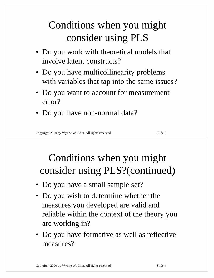
Copyright 2000 by Wynne W. Chin. All rights reserved. Slide 3
Conditions when you might consider using PLS
• Do you work with theoretical models that involve latent constructs?
• Do you have multicollinearity problems with variables that tap into the same issues?
• Do you want to account for measurement error?
• Do you have non-normal data?
Copyright 2000 by Wynne W. Chin. All rights reserved. Slide 4
Conditions when you might consider using PLS?(continued)
• Do you have a small sample set?• Do you wish to determine whether the
measures you developed are valid and reliable within the context of the theory you are working in?
• Do you have formative as well as reflective measures?

Copyright 2000 by Wynne W. Chin. All rights reserved. Slide 5
Being a component approach, PLS covers:
• principal component, • multiple regression• canonical correlation, • redundancy, • inter-battery factor, • multi-set canonical correlation, and• correspondence analysis as special cases
Copyright 2000 by Wynne W. Chin. All rights reserved. Slide 6
PLS
Redundancy Analysis
ESSCA Canonical Correlation
Multiple Regression
Multiple Discriminant
Analysis
Analysis of Variance
Analysis of Covariance
Principal Components
Simultaneous Equations
Factor Analysis
Covariance Based SEM
A B means B is a special case of A
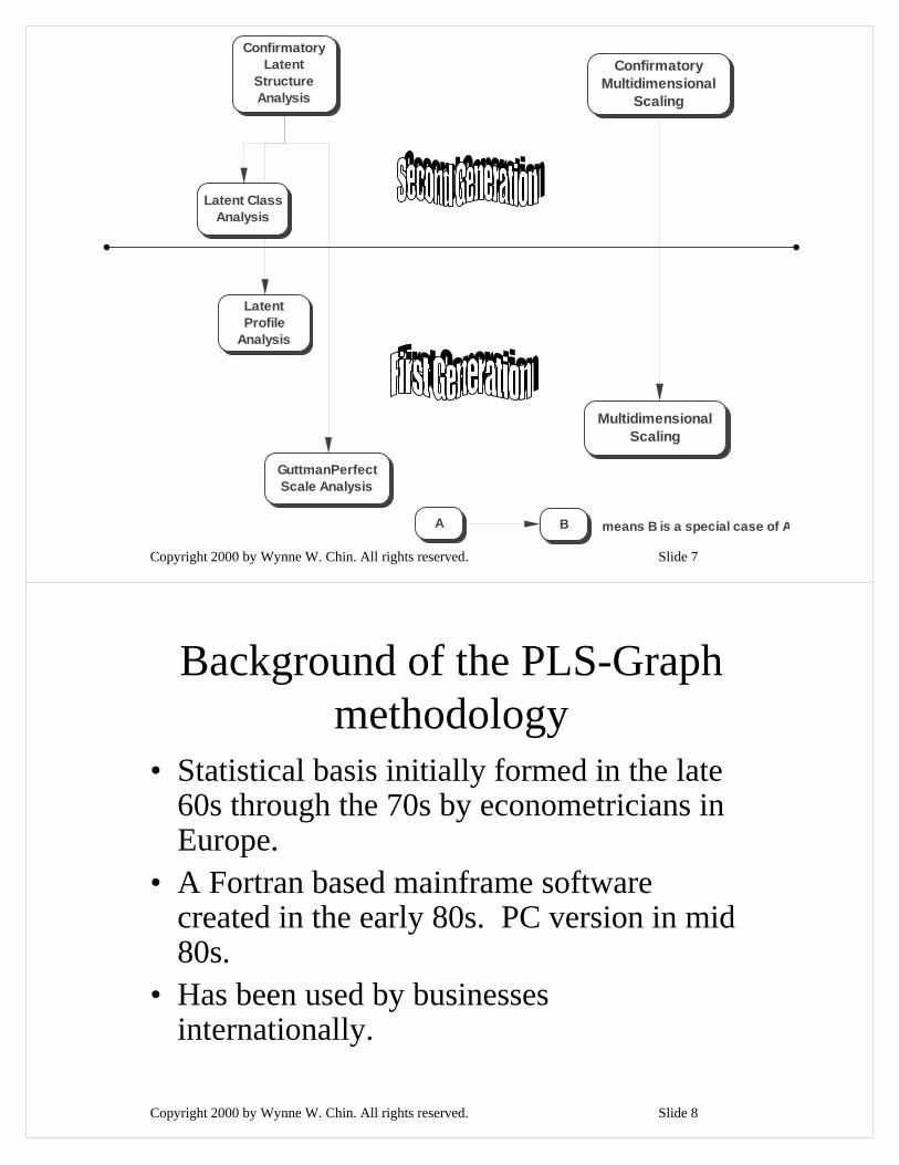
Copyright 2000 by Wynne W. Chin. All rights reserved. Slide 7
Confirmatory Latent
Structure Analysis
Latent Class Analysis
Latent Profile
Analysis
GuttmanPerfect Scale Analysis
Confirmatory Multidimensional
Scaling
Multidimensional Scaling
A B means B is a special case of A
Copyright 2000 by Wynne W. Chin. All rights reserved. Slide 8
Background of the PLS-Graph methodology
• Statistical basis initially formed in the late 60s through the 70s by econometricians in Europe.
• A Fortran based mainframe software created in the early 80s. PC version in mid 80s.
• Has been used by businesses internationally.

Copyright 2000 by Wynne W. Chin. All rights reserved. Slide 9
Background of the PLS-Graph methodology (continued)
• The PLS-Graph software has been under development for the past 8 years. Academic beta testers include Queens University, Western Ontario, UBC, MIT,UCF, AGSM, U of Michigan, U of Illinois, Florida State, National University of Singapore, NTU, Ohio State, Wharton, UCLA, Georgia State, the University of Houston, and City U of Hong Kong.
Copyright 2000 by Wynne W. Chin. All rights reserved. Slide 10“But we just don’t have the technology to carry it out.”

Copyright 2000 by Wynne W. Chin. All rights reserved. Slide 11
Let’s See How It Works
Copyright 2000 by Wynne W. Chin. All rights reserved. Slide 12
INTENTION
VINT1 I presently intend to use Voice Mailregularly:
VINT2 My actual intention to use Voice Mailregularly is:
VINT3 Once again, to what extent do you at presentintend to use Voice Mail regularly:
Copyright 2000 by Wynne W. Chin. All rights reserved. Slide 13
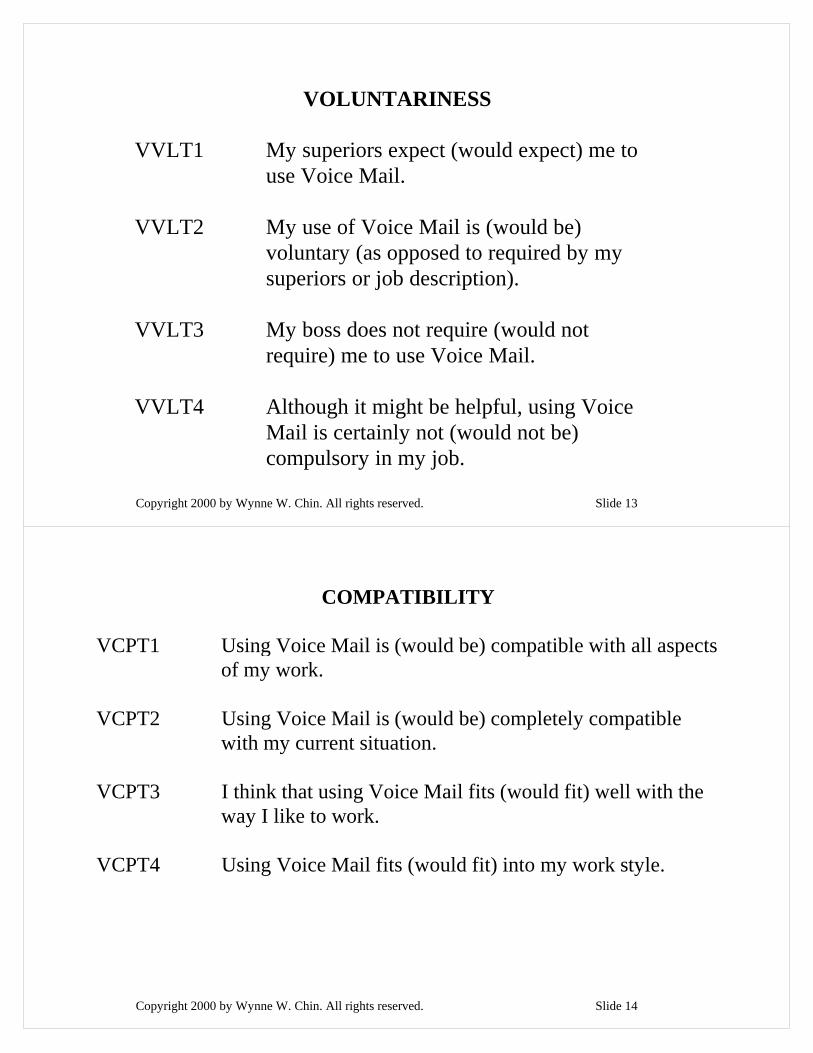
VOLUNTARINESS
VVLT1 My superiors expect (would expect) me touse Voice Mail.
VVLT2 My use of Voice Mail is (would be)voluntary (as opposed to required by mysuperiors or job description).
VVLT3 My boss does not require (would notrequire) me to use Voice Mail.
VVLT4 Although it might be helpful, using VoiceMail is certainly not (would not be)compulsory in my job.
Copyright 2000 by Wynne W. Chin. All rights reserved. Slide 14
COMPATIBILITY VCPT1 Using Voice Mail is (would be) compatible with all aspects
of my work. VCPT2 Using Voice Mail is (would be) completely compatible
with my current situation. VCPT3 I think that using Voice Mail fits (would fit) well with the
way I like to work. VCPT4 Using Voice Mail fits (would fit) into my work style.
Copyright 2000 by Wynne W. Chin. All rights reserved. Slide 15
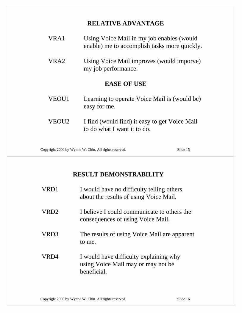
RELATIVE ADVANTAGE
VRA1 Using Voice Mail in my job enables (wouldenable) me to accomplish tasks more quickly.
VRA2 Using Voice Mail improves (would imporve)my job performance.
EASE OF USE
VEOU1 Learning to operate Voice Mail is (would be)easy for me.
VEOU2 I find (would find) it easy to get Voice Mailto do what I want it to do.
Copyright 2000 by Wynne W. Chin. All rights reserved. Slide 16
RESULT DEMONSTRABILITY VRD1 I would have no difficulty telling others
about the results of using Voice Mail. VRD2 I believe I could communicate to others the
consequences of using Voice Mail. VRD3 The results of using Voice Mail are apparent
to me. VRD4 I would have difficulty explaining why
using Voice Mail may or may not be beneficial.
Copyright 2000 by Wynne W. Chin. All rights reserved. Slide 17
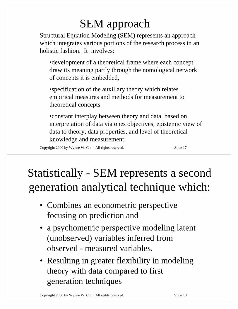
SEM approachStructural Equation Modeling (SEM) represents an approach which integrates various portions of the research process in an holistic fashion. It involves:
•development of a theoretical frame where each concept draw its meaning partly through the nomological network of concepts it is embedded,
•specification of the auxillary theory which relates empirical measures and methods for measurement to theoretical concepts
•constant interplay between theory and data based on interpretation of data via ones objectives, epistemic view of data to theory, data properties, and level of theoretical knowledge and measurement.
Copyright 2000 by Wynne W. Chin. All rights reserved. Slide 18
Statistically - SEM represents a second generation analytical technique which:
• Combines an econometric perspective focusing on prediction and
• a psychometric perspective modeling latent(unobserved) variables inferred from observed - measured variables.
• Resulting in greater flexibility in modeling theory with data compared to first generation techniques
Copyright 2000 by Wynne W. Chin. All rights reserved. Slide 19
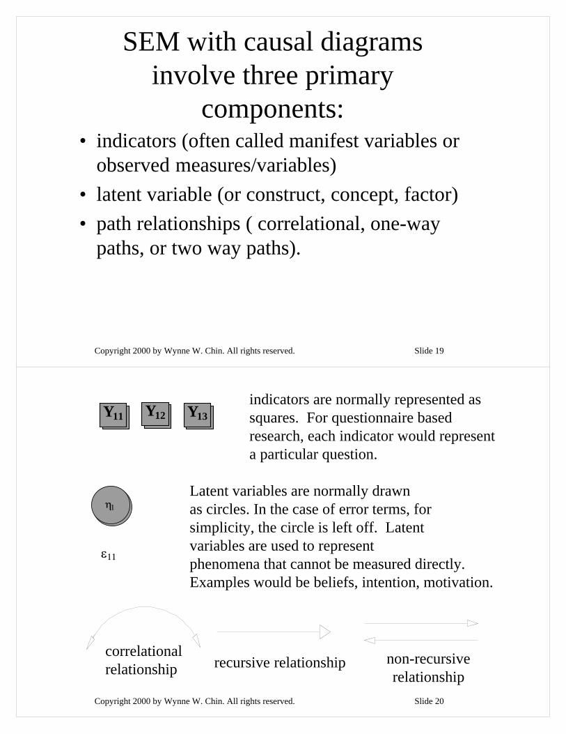
• indicators (often called manifest variables or observed measures/variables)
• latent variable (or construct, concept, factor)• path relationships ( correlational, one-way
paths, or two way paths).
SEM with causal diagrams involve three primary
components:
Copyright 2000 by Wynne W. Chin. All rights reserved. Slide 20
Y11 Y12 Y13indicators are normally represented as squares. For questionnaire based research, each indicator would representa particular question.
η1Latent variables are normally drawnas circles. In the case of error terms, for simplicity, the circle is left off. Latent variables are used to representphenomena that cannot be measured directly.Examples would be beliefs, intention, motivation.
ε11
correlationalrelationship recursive relationship non-recursive
relationship
Copyright 2000 by Wynne W. Chin. All rights reserved. Slide 21
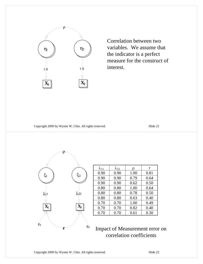
ρ
1.0 1.0
η1
X1
η2
X2
Correlation between twovariables. We assume thatthe indicator is a perfect measure for the construct ofinterest.
Copyright 2000 by Wynne W. Chin. All rights reserved. Slide 22
ε
λ11
ρ
λ22
r
ξ1
X1
ξ2
X2
ε11
λ11 λ22 ρ r0.90 0.90 1.00 0.810.90 0.90 0.79 0.640.90 0.90 0.62 0.500.80 0.80 1.00 0.640.80 0.80 0.78 0.500.80 0.80 0.63 0.400.70 0.70 1.00 0.490.70 0.70 0.82 0.400.70 0.70 0.61 0.30
Impact of Measurement error oncorrelation coefficients
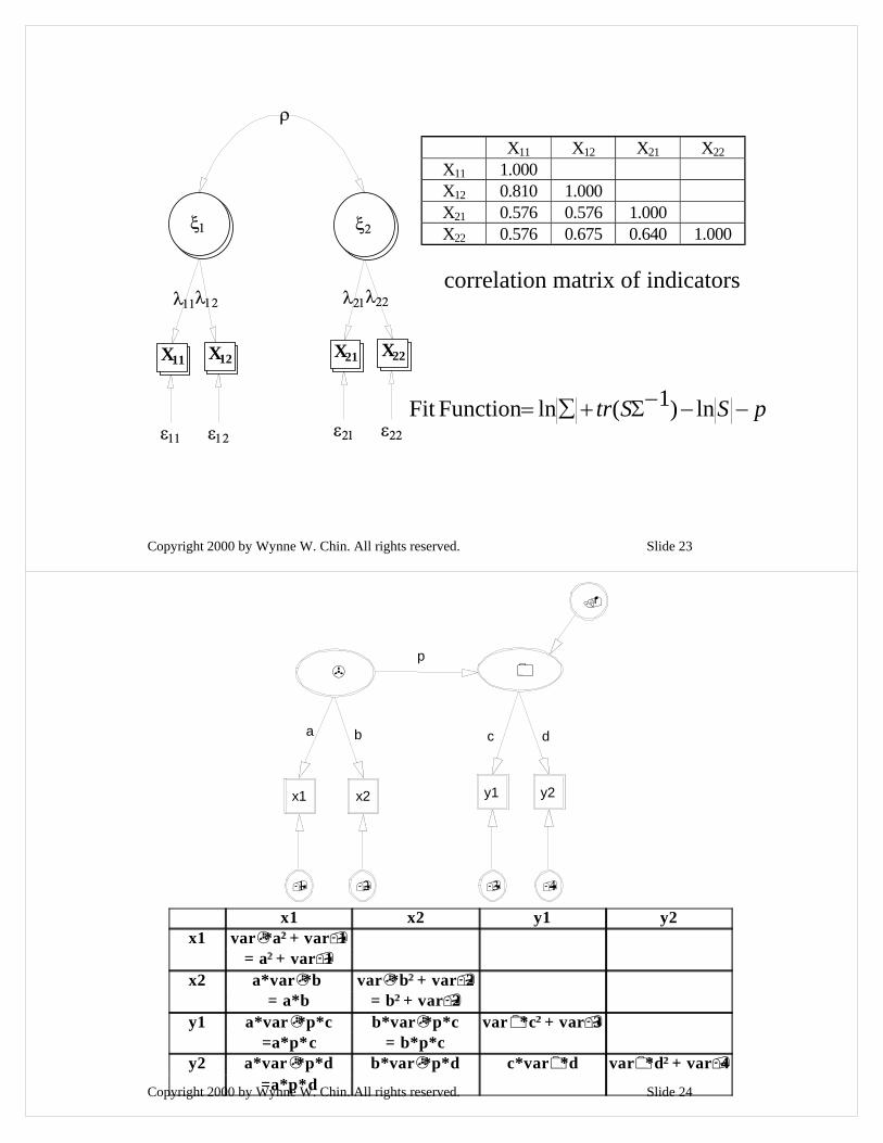
Copyright 2000 by Wynne W. Chin. All rights reserved. Slide 23
ρ
λ11λ12 λ21λ22
ξ1 ξ2
X11
ε11
X12
ε12
X21
ε21
X22
ε22
X11 X12 X21 X22X11 1.000X12 0.810 1.000X21 0.576 0.576 1.000X22 0.576 0.675 0.640 1.000
correlation matrix of indicators
pSStr −−−Σ+∑= ln)1(lnFunction Fit
Copyright 2000 by Wynne W. Chin. All rights reserved. Slide 24
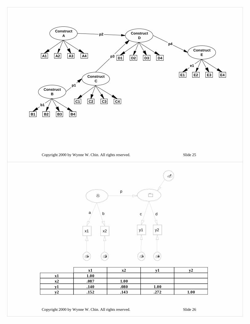
x1 x2 y1 y2x1 var *a2 2 + var 1
= a2 2 + var 1x2 a*var *b
= a*bvar *b2 2 + var 2
= b2 2 + var 2y1 a*var *p*c
=a*p*cb*var *p*c
= b*p*cvar *c2 2 + var 3
y2 a*var *p*d=a*p*d
b*var *p*d c*var *d var *d2 2 + var 4
p
a b c d
x1 x2 y1 y2
1 2 3 4
Copyright 2000 by Wynne W. Chin. All rights reserved. Slide 25
b1
e1
p1
p2
p3
p4
Construct D
D1 D2 D3 D4
Construct A
A1 A2 A3 A4
Construct B
B1 B2 B3 B4
Construct E
E1 E2 E3 E4Construct C
C1 C2 C3 C4
Copyright 2000 by Wynne W. Chin. All rights reserved. Slide 26
x1 x2 y1 y2x1 1.00x2 .087 1.00y1 .140 .080 1.00y2 .152 .143 .272 1.00
p
a b c d
x1 x2 y1 y2
1 2 3 4
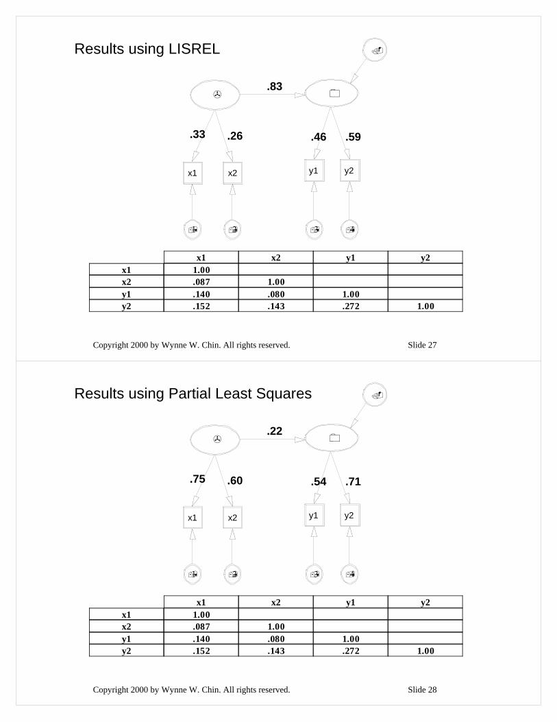
Copyright 2000 by Wynne W. Chin. All rights reserved. Slide 27
.83
.33 .26 .46 .59
x1 x2 y1 y2
1 2 3 4
Results using LISREL
x1 x2 y1 y2x1 1.00x2 .087 1.00y1 .140 .080 1.00y2 .152 .143 .272 1.00
Copyright 2000 by Wynne W. Chin. All rights reserved. Slide 28
.22
.75 .60 .54 .71
x1 x2 y1 y2
1 2 3 4
x1 x2 y1 y2x1 1.00x2 .087 1.00y1 .140 .080 1.00y2 .152 .143 .272 1.00
Results using Partial Least Squares
Copyright 2000 by Wynne W. Chin. All rights reserved. Slide 29
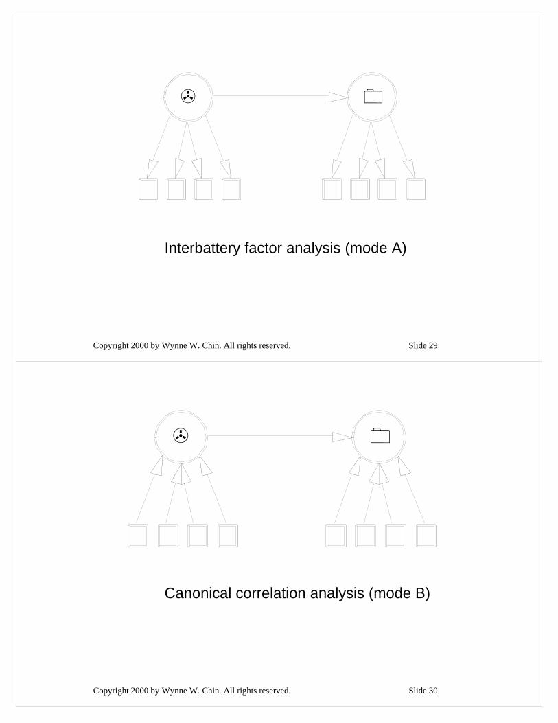
Interbattery factor analysis (mode A)
Copyright 2000 by Wynne W. Chin. All rights reserved. Slide 30
Canonical correlation analysis (mode B)
Copyright 2000 by Wynne W. Chin. All rights reserved. Slide 31
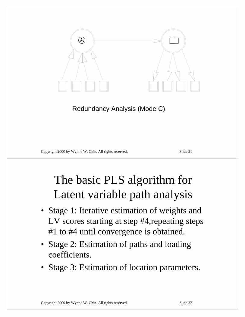
Redundancy Analysis (Mode C).
Copyright 2000 by Wynne W. Chin. All rights reserved. Slide 32
The basic PLS algorithm for Latent variable path analysis
• Stage 1: Iterative estimation of weights and LV scores starting at step #4,repeating steps #1 to #4 until convergence is obtained.
• Stage 2: Estimation of paths and loading coefficients.
• Stage 3: Estimation of location parameters.
Copyright 2000 by Wynne W. Chin. All rights reserved. Slide 33
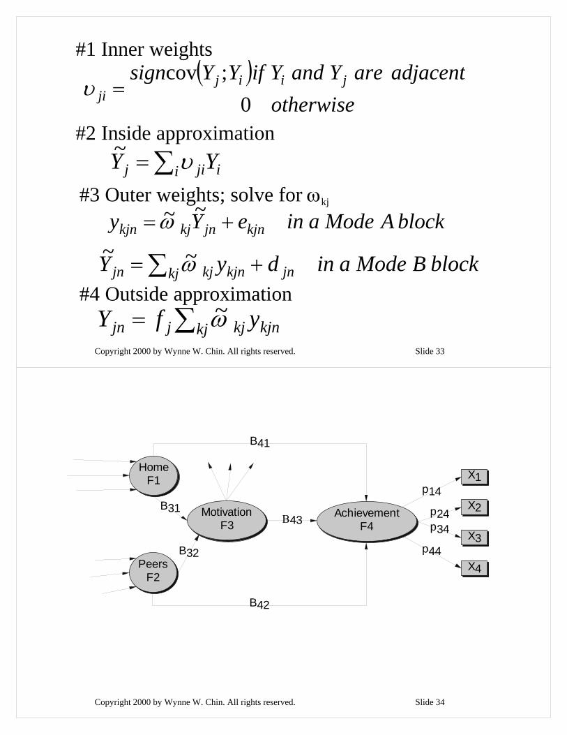
( )otherwise
adjacentareYandYifYYsign jiijji 0
;cov=υ
∑= i ijij YY υ~
blockAModeaineYy kjnjnkjkjn += ~~ω
blockBModeaindyY jnkj kjnkjjn += ∑ ω~~
#1 Inner weights
#2 Inside approximation
#3 Outer weights; solve for ωkj
∑= kj kjnkjjjn yfY ω~#4 Outside approximation
Copyright 2000 by Wynne W. Chin. All rights reserved. Slide 34
p14
p24p34
p44
Β43B31
B32
B41
B42
HomeF1
PeersF2
MotivationF3
AchievementF4
X1
X2
X3
X4

Copyright 2000 by Wynne W. Chin. All rights reserved. Slide 35
Latent Construct
Emergent Construct
Reflective indicators Formative indicators
Latent or Emergent Constructs?
Parental Monitoring Ability•eyesight•overall physical health•number of children being monitored•motivation to monitor
Parental Monitoring Ability•self-reported evaluation•video taped measured time•child’s assessment•external expert
Copyright 2000 by Wynne W. Chin. All rights reserved. Slide 36
Reflective indicators Formative indicators
Latent or Emergent Constructs?
Parental Monitoring Ability•eyesight•overall physical health•number of children being monitored•motivation to monitor
Parental Monitoring Ability•self-reported evaluation•video taped measured time•child’s assessment•external expert
These measures should covary.•If a parent behaviorally increased their monitoring ability- each measure should increase
as well.
These measures need not covary.•A drop in health need not imply any change in number of children being monitored. •Measures of internal consistency do not apply.
Copyright 2000 by Wynne W. Chin. All rights reserved. Slide 37
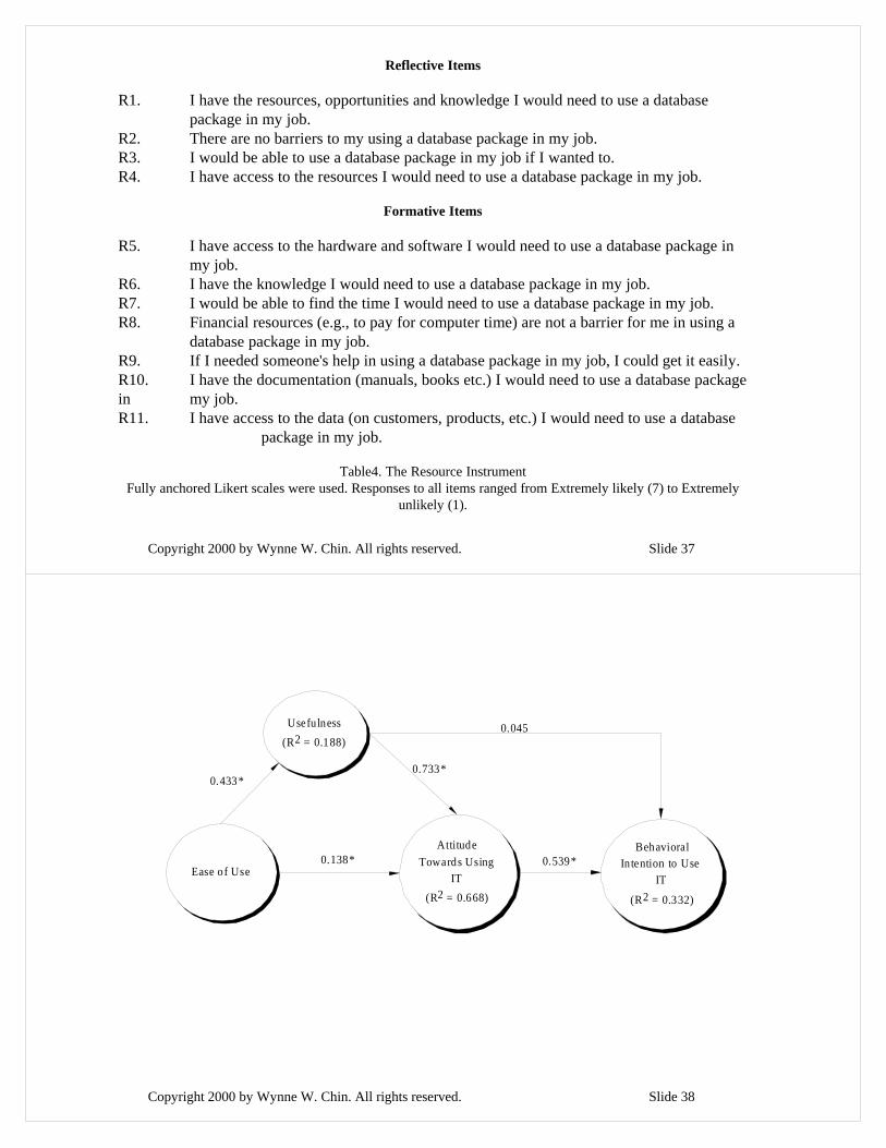
Reflective Items
R1. I have the resources, opportunities and knowledge I would need to use a database package in my job.
R2. There are no barriers to my using a database package in my job.R3. I would be able to use a database package in my job if I wanted to.R4. I have access to the resources I would need to use a database package in my job.
Formative Items
R5. I have access to the hardware and software I would need to use a database package in my job.
R6. I have the knowledge I would need to use a database package in my job.R7. I would be able to find the time I would need to use a database package in my job.R8. Financial resources (e.g., to pay for computer time) are not a barrier for me in using a
database package in my job.R9. If I needed someone's help in using a database package in my job, I could get it easily.R10. I have the documentation (manuals, books etc.) I would need to use a database package in my job.R11. I have access to the data (on customers, products, etc.) I would need to use a database
package in my job.
Table4. The Resource InstrumentFully anchored Likert scales were used. Responses to all items ranged from Extremely likely (7) to Extremely
unlikely (1).
Copyright 2000 by Wynne W. Chin. All rights reserved. Slide 38
0.539*0.138*
0.433*0.733*
0.045
Behavioral In tention to Use
IT
(R2 = 0.332)
Attitude Towards Using
IT(R2 = 0.668)
Usefulness(R2 = 0.188)
Ease of Use
Copyright 2000 by Wynne W. Chin. All rights reserved. Slide 39
0.589*(0.930)
0.270*(0.814)
0.100*(0.735)
0.027(0.566)
0.132*(0.654)
-0.022(0.546)
0.118(0.602)
0.873*
0.893*(0.271)
0.904*(0.261)
0.911*(0.274)
0.903*(0.310)
Resources formative
Resources reflective
R5. Hardware/Software
R6. Knowledge
R7. Time
R8. Financial Resources
R9. Someone's Help
R10. Documentation
R11. Data
R1 R2 R3 R4
Figure 7. Redundancy analysis of perceived resources ( * indicates significant estimates).
Copyright 2000 by Wynne W. Chin. All rights reserved. Slide 40
0.216*
0.453*0.107
0.322*0.733*
0.003
0.076*
0.510*
0.291*
Behavioral Intention to
Use IT(R2 = 0.402)
Attitude Towards Using IT
(R2 = 0.673)
Usefulness
(R2 = 0.222)
Ease of Use
(R2 = 0.260)
Resources(reflective)
Copyright 2000 by Wynne W. Chin. All rights reserved. Slide 41
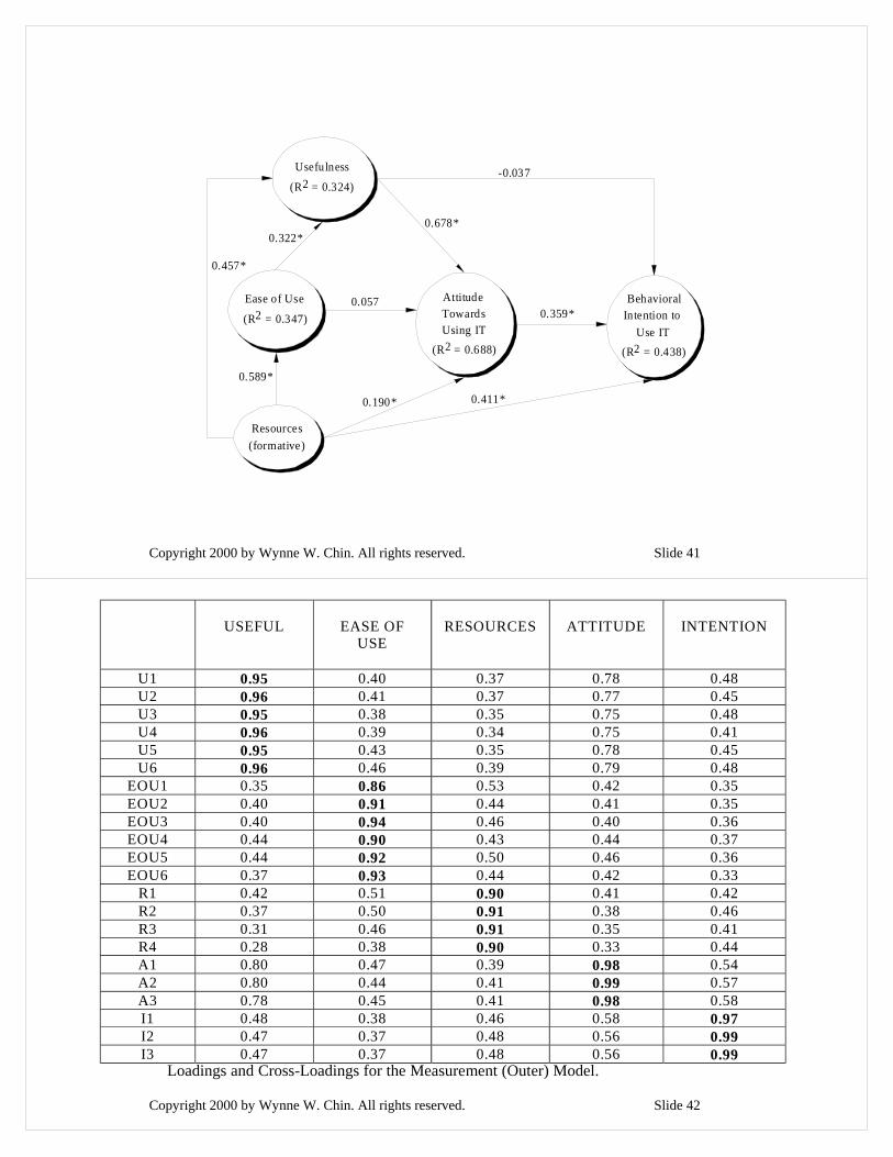
0.457*
0.359*0.057
0.322*0.678*
-0.037
0.190*
0.589*
0.411*
Behavioral Intention to
Use IT(R2 = 0.438)
Attitude Towards Using IT
(R2 = 0.688)
Usefulness
(R2 = 0.324)
Ease of Use
(R2 = 0.347)
Resources(formative)
Copyright 2000 by Wynne W. Chin. All rights reserved. Slide 42
Loadings and Cross-Loadings for the Measurement (Outer) Model.
USEFUL EASE OFUSE
RESOURCES ATTITUDE INTENTION
U1 0.95 0.40 0.37 0.78 0.48U2 0.96 0.41 0.37 0.77 0.45U3 0.95 0.38 0.35 0.75 0.48U4 0.96 0.39 0.34 0.75 0.41U5 0.95 0.43 0.35 0.78 0.45U6 0.96 0.46 0.39 0.79 0.48
EOU1 0.35 0.86 0.53 0.42 0.35EOU2 0.40 0.91 0.44 0.41 0.35EOU3 0.40 0.94 0.46 0.40 0.36EOU4 0.44 0.90 0.43 0.44 0.37EOU5 0.44 0.92 0.50 0.46 0.36EOU6 0.37 0.93 0.44 0.42 0.33
R1 0.42 0.51 0.90 0.41 0.42R2 0.37 0.50 0.91 0.38 0.46R3 0.31 0.46 0.91 0.35 0.41R4 0.28 0.38 0.90 0.33 0.44A1 0.80 0.47 0.39 0.98 0.54A2 0.80 0.44 0.41 0.99 0.57A3 0.78 0.45 0.41 0.98 0.58I1 0.48 0.38 0.46 0.58 0.97I2 0.47 0.37 0.48 0.56 0.99I3 0.47 0.37 0.48 0.56 0.99
Copyright 2000 by Wynne W. Chin. All rights reserved. Slide 43
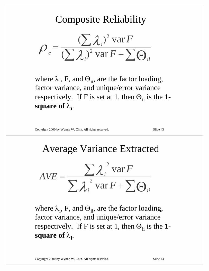
Composite Reliability
∑Θ∑∑
+=
iii
ic F
Fvar
var2
2
)()(
λλρ
where λi, F, and Θii, are the factor loading, factor variance, and unique/error variance respectively. If F is set at 1, then Θii is the 1-square of λi.
Copyright 2000 by Wynne W. Chin. All rights reserved. Slide 44
Average Variance Extracted
∑Θ∑∑
+=
iii
i
FF
AVEvar
var2
2
λλ
where λi, F, and Θii, are the factor loading, factor variance, and unique/error variance respectively. If F is set at 1, then Θii is the 1-square of λi.
Copyright 2000 by Wynne W. Chin. All rights reserved. Slide 45
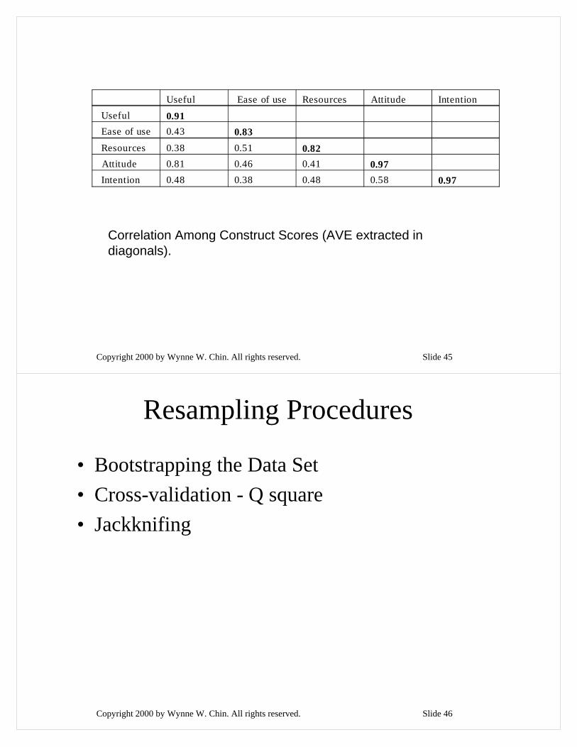
Useful Ease of use Resources Attitude Intention Useful 0.91 Ease of use 0.43 0.83 Resources 0.38 0.51 0.82 Attitude 0.81 0.46 0.41 0.97 Intention 0.48 0.38 0.48 0.58 0.97
Correlation Among Construct Scores (AVE extracted in diagonals).
Copyright 2000 by Wynne W. Chin. All rights reserved. Slide 46
Resampling Procedures
• Bootstrapping the Data Set• Cross-validation - Q square• Jackknifing
Copyright 2000 by Wynne W. Chin. All rights reserved. Slide 47
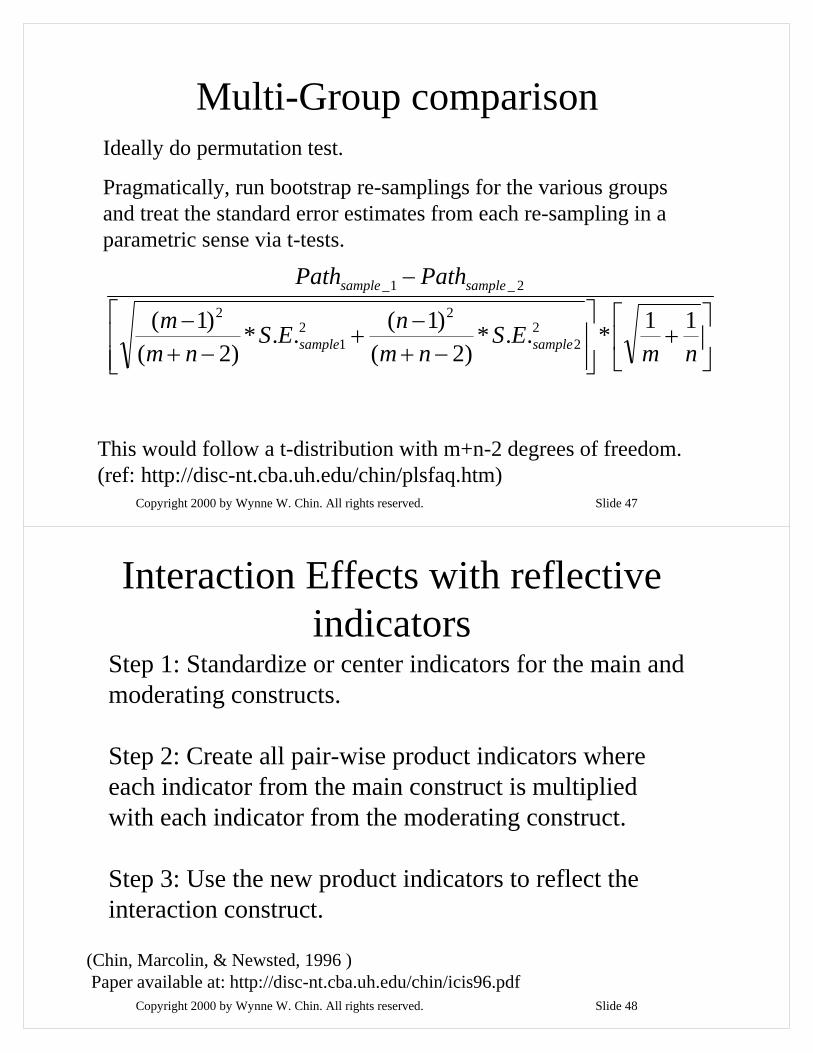
Multi-Group comparisonIdeally do permutation test.
Pragmatically, run bootstrap re-samplings for the various groups and treat the standard error estimates from each re-sampling in a parametric sense via t-tests.
⎥⎦
⎤⎢⎣
⎡+
⎥⎥⎦
⎤
⎢⎢⎣
⎡
−+−
+−+
−
−
nmES
nmnES
nmm
PathPath
samplesample
samplesample
11*..*)2(
)1(..*)2(
)1( 22
22
1
2
2_1_
This would follow a t-distribution with m+n-2 degrees of freedom.(ref: http://disc-nt.cba.uh.edu/chin/plsfaq.htm)
Copyright 2000 by Wynne W. Chin. All rights reserved. Slide 48
Interaction Effects with reflective indicators
(Chin, Marcolin, & Newsted, 1996 )Paper available at: http://disc-nt.cba.uh.edu/chin/icis96.pdf
Step 1: Standardize or center indicators for the main and moderating constructs.
Step 2: Create all pair-wise product indicators where each indicator from the main construct is multiplied with each indicator from the moderating construct.
Step 3: Use the new product indicators to reflect the interaction construct.

Copyright 2000 by Wynne W. Chin. All rights reserved. Slide 49
XPredictor Variable
X*ZInteraction
Effect
x1 x2 x3
ZModerator
Variable
z1 z2 z3
YDependent
Variable
y1 y2 y3
x2*z1 x2*z2 x2*z3 x3*z1 x3*z2 x3*z3x1*z1 x1*z2 x1*z3
Copyright 2000 by Wynne W. Chin. All rights reserved. Slide 50
Indicators per construct Sample
size one item
per construct
two per construct
(4 for interaction)
four per construct (16 for
interaction)
six per construct (36 for
interaction)
eight per construct (64 for
interaction)
ten per construct (100 for
interaction)
twelve per construct (144 for
interaction)20
0.1458
(0.2852) 0.1609
(0.3358) 0.2708
(0.3601) 0.1897
(0.4169) 0.1988
(0.4399) 0.2788
(0.3886) 0.3557
(0.3725) 50
0.1133
(0.1604) 0.1142
(0.2124) 0.2795
(0.1873) 0.2403
(0.2795) 0.3066
(0.2183) 0.3083
(0.2707) 0.3615 (0.1848)
100
0.1012 (0.0989)
0.1614 (0.1276)
0.2472 (0.1270)
0.2669 (0.1301)
0.3029 (0.0916)
0.3029 (0.0805)
0.3008 (0.1352)
150
0.0953 (0.0843)
0.1695 (0.0844)
0.2427 (0.0778)
0.2834 (0.0757)
0.2805 (0.0916)
0.3040 (0.0567)
0.2921 (0.0840)
200
0.0962 (0.0785)
0.1769 (0.0674)
0.2317 (0.0543)
0.2730 (0.0528)
0.2839 (0.0606)
0.2843 (0.0573)
0.3018 (0.0542)
500
0.0965 (0.0436)
0.1681 (0.0358)
0.2275 (0.0419)
0.2448 (0.0379)
0.2637 (0.0377)
0.2659 (0.0353)
0.2761 (0.0375)
Results from Monte Carlo Simulation
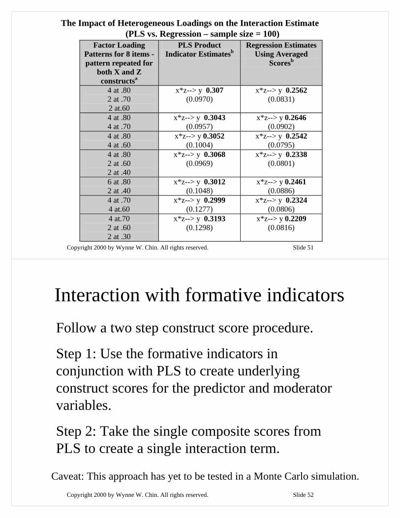
Copyright 2000 by Wynne W. Chin. All rights reserved. Slide 51
Factor Loading Patterns for 8 items - pattern repeated for
both X and Z constructsa
PLS Product Indicator Estimatesb
Regression Estimates Using Averaged
Scoresb
4 at .80 2 at .70 2 at.60
x*z--> y 0.307 (0.0970)
x*z--> y 0.2562 (0.0831)
4 at .80 4 at .70
x*z--> y 0.3043 (0.0957)
x*z--> y 0.2646 (0.0902)
4 at .80 4 at .60
x*z--> y 0.3052 (0.1004)
x*z--> y 0.2542 (0.0795)
4 at .80 2 at .60 2 at .40
x*z--> y 0.3068 (0.0969)
x*z--> y 0.2338 (0.0801)
6 at .80 2 at .40
x*z--> y 0.3012 (0.1048)
x*z--> y 0.2461 (0.0886)
4 at .70 4 at.60
x*z--> y 0.2999 (0.1277)
x*z--> y 0.2324 (0.0806)
4 at.70 2 at .60 2 at .30
x*z--> y 0.3193 (0.1298)
x*z--> y 0.2209 (0.0816)
The Impact of Heterogeneous Loadings on the Interaction Estimate(PLS vs. Regression – sample size = 100)
Copyright 2000 by Wynne W. Chin. All rights reserved. Slide 52
Interaction with formative indicatorsFollow a two step construct score procedure.
Step 1: Use the formative indicators in conjunction with PLS to create underlying construct scores for the predictor and moderator variables.
Step 2: Take the single composite scores from PLS to create a single interaction term.
Caveat: This approach has yet to be tested in a Monte Carlo simulation.
Copyright 2000 by Wynne W. Chin. All rights reserved. Slide 53
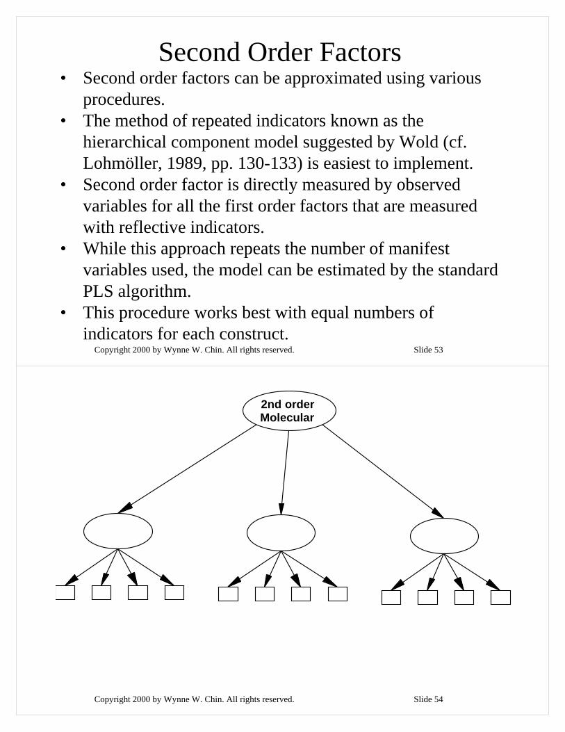
Second Order Factors• Second order factors can be approximated using various
procedures. • The method of repeated indicators known as the
hierarchical component model suggested by Wold (cf. Lohmöller, 1989, pp. 130-133) is easiest to implement.
• Second order factor is directly measured by observed variables for all the first order factors that are measured with reflective indicators.
• While this approach repeats the number of manifest variables used, the model can be estimated by the standard PLS algorithm.
• This procedure works best with equal numbers of indicators for each construct.
Copyright 2000 by Wynne W. Chin. All rights reserved. Slide 54
2nd order Molecular

Copyright 2000 by Wynne W. Chin. All rights reserved. Slide 55
2nd Order Molar
Copyright 2000 by Wynne W. Chin. All rights reserved. Slide 56
Considerations when choosing between PLS and LISREL
• Objectives• Theoretical constructs - indeterminate vs.
defined• Epistemic relationships• Theory requirements• Empirical factors• Computational issues - identification &
speed
Copyright 2000 by Wynne W. Chin. All rights reserved. Slide 57
Objectives
• Prediction versus explanation
Copyright 2000 by Wynne W. Chin. All rights reserved. Slide 58
Theoretical constructs -Indeterminate versus defined
• For PLS - the latent variables are estimated as linear aggregates or components. The latent variable scores are estimated directly. If raw data is used, scoring coefficients are estimated.
• For LISREL - Indeterminacy
Copyright 2000 by Wynne W. Chin. All rights reserved. Slide 59
Epistemic relationships• Latent constructs with reflective indicators -
LISREL & PLS• Emergent constructs with formative
indicators - PLS• By choosing different weighting “modes”
the model builder shifts the emphasis of the model from a structural causal explanation of the covariance matrix to a prediction/reconstruction forecast of the raw data matrix
Copyright 2000 by Wynne W. Chin. All rights reserved. Slide 60
Theory requirements
• LISREL expects strong theory (confirmation mode)
• PLS is flexible
Copyright 2000 by Wynne W. Chin. All rights reserved. Slide 61
Empirical factors
• Distributional assumptions– PLS estimation is a “rigid” technique that
requires only “soft” assumptions about the distributional characteristics of the raw data.
– LISREL requires more stringent conditions.
Copyright 2000 by Wynne W. Chin. All rights reserved. Slide 62
Empirical factors (continued)• Sample Size depends on power analysis, but
much smaller for PLS– PLS heuristic of ten times the greater of the
following two (ideally use power analysis)• construct with the greatest number of formative
indicators• construct with the greatest number of structural paths
going into it
– LISREL heuristic - at least 200 cases or 10 times the number of parameters estimated.
Copyright 2000 by Wynne W. Chin. All rights reserved. Slide 63
Empirical factors (continued)• Types of measures
– PLS can use categorical through ratio measures– LISREL generally expects interval level,
otherwise need PRELIS preprocessing.
Copyright 2000 by Wynne W. Chin. All rights reserved. Slide 64
Computational issues -Identification
• Are estimates unique?• Under recursive models - PLS is always
identified• LISREL - depends on the model. Ideally
need 4 or more indicators per construct to be over determined, 3 to be just identified. Algebraic proof for identification.
Copyright 2000 by Wynne W. Chin. All rights reserved. Slide 65
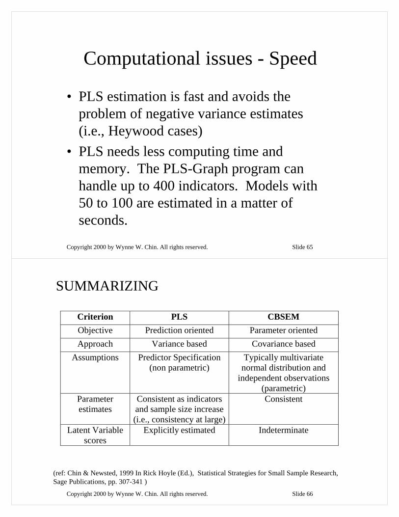
Computational issues - Speed
• PLS estimation is fast and avoids the problem of negative variance estimates (i.e., Heywood cases)
• PLS needs less computing time and memory. The PLS-Graph program can handle up to 400 indicators. Models with 50 to 100 are estimated in a matter of seconds.
Copyright 2000 by Wynne W. Chin. All rights reserved. Slide 66
Criterion PLS CBSEM Objective Prediction oriented Parameter oriented Approach Variance based Covariance based
Assumptions Predictor Specification (non parametric)
Typically multivariate normal distribution and
independent observations (parametric)
Parameter estimates
Consistent as indicators and sample size increase (i.e., consistency at large)
Consistent
Latent Variable scores
Explicitly estimated Indeterminate
(ref: Chin & Newsted, 1999 In Rick Hoyle (Ed.), Statistical Strategies for Small Sample Research, Sage Publications, pp. 307-341 )
SUMMARIZING

Copyright 2000 by Wynne W. Chin. All rights reserved. Slide 67
Criterion PLS CBSEM Epistemic
relationship between a latent variable and its
measures
Can be modeled in either
formative or reflective mode
Typically only with reflective indicators
Implications Optimal for prediction accuracy
Optimal for parameter accuracy
Model Complexity
Large complexity (e.g., 100 constructs and 1000
indicators)
Small to moderate complexity (e.g., less than
100 indicators)
Sample Size Power analysis based on the portion of the model with the largest number of predictors. Minimal recommendations range from 30 to 100 cases.
Ideally based on power analysis of specific model - minimal recommendations
range from 200 to 800.
(ref: Chin & Newsted, 1999 In Rick Hoyle (Ed.), Statistical Strategies for Small Sample Research, Sage Publications, pp. 307-341 )
SUMMARIZING
Copyright 2000 by Wynne W. Chin. All rights reserved. Slide 68
Additional Questions?
Slides will be available after December 20th at:http://disc-nt.cba.uh.edu/chin/indx.html