Parameter-Estimation Algorithms for Characterizing a...

Mechanics of Time-Dependent Materials 6: 323–362, 2002.© 2002 Kluwer Academic Publishers. Printed in the Netherlands.

323

Parameter-Estimation Algorithms forCharacterizing a Class of Isotropic andAnisotropic Viscoplastic Material Models

A.F. SALEEB1, A.S. GENDY2 and T.E. WILT1

1Civil Engineering Department, The University of Akron, Akron, OH 44325, U.S.A.2Structural Engineering Department, Faculty of Engineering, Cairo University, Giza, Egypt

(Received 16 October 2001; accepted in revised form 9 August 2002)

Abstract. A number of robust, and computationally efficient, algorithms are presented for thedevelopment of an overall strategy to estimate the material parameters characterizing a class of com-plex viscoplastic material models (i.e., rate dependent plastic flow, nonlinear kinematic hardening,thermal/static recovery, isotropic and anisotropic, etc.). The entire procedure is automated throughthe integrated software COMPARE (an acronym for COnstitutive Material PARameter Estimator)to enable the determination of an ‘optimum’ set of material parameters by minimizing the errorsbetween the experimental test data and the predicted response. The key ingredients of COMPAREare: (i) primal analysis utilizing the unconditionally-stable, fully implicit, integration scheme forthe models’ underlying flow and evolutionary rate equations; (ii) sensitivity analysis utilizing adirect-differentiation approach (i.e., explicit, ‘exact’ expressions are derived); (iii) a gradient-basedoptimization technique of an error/cost function; and (iv) graphical user interface. The estimation ofthe material parameters is cast as a minimum-error, weighted-multi-objective, nonlinear optimizationproblem with constraints. Comparison between the sensitivities obtained by the proposed directscheme and those produced by conventional finite difference techniques is presented to assess ac-curacy. Detailed derivations are given, together with the results generated by applying the developedalgorithms to a comprehensive set of test matrices. These include constant strain-rate tension, creep,and relaxation tests, for both isotropic as well as anisotropic behaviors.

Key words: experimental test data, implicit sensitivities, material characterization, multi-objectiveoptimization technique, parameter estimation, time-dependence, viscoplastic constitutive model

1. Introduction

1.1. GENERAL

Significant progress has been made over the years in the development of theories ofplasticity and viscoplasticity for the phenomenological representations of inelasticconstitutive properties. In particular, the mathematical modeling of metal visco-plasticity is presently very well developed, based on the so-called internal variableformulism in the thermodynamics of irreversible processes (Coleman and Gurtin,1967; Lubliner, 1973; Lemaitre and Chaboche, 1990; Chaboche, 1989; Arnoldand Saleeb, 1994; Arnold et al., 1995; Freed and Walker, 1993). A number of

324 A.F. SALEEB ET AL.

specialized forms of these modern unified viscoplastic models (e.g., isotropic andanisotropic, fully associative and nonassociative, isothermal or nonisothermal, etc.)have been successfully applied to different metals and composite material systems(Lemaitre and Chaboche, 1990; Chaboche, 1989; Arnold et al., 1995; Freed andWalker, 1993; Robinson and Duffy, 1990; Robinson et al., 1987). Naturally, thebetter accuracy and improved modeling capabilities in these representations haveoften been acquired at the expense of greater mathematical complexity and a lar-ger number of material parameters. Such material parameters are often introducedto describe a host of physical phenomena and complicated deformation mechan-isms. The experimental characterization of these material parameters constitutesa major factor in the successful and effective utilization of any given constitutivemodel; i.e., the problem of constitutive parameter estimation from experimentalmeasurements.

In mathematical terminology, this constitutes an inverse problem (e.g., Bui andTanaka, 1994), for the simultaneous identification of a large number of paramet-ers from comprehensive test matrices (i.e., under different loading conditions andcontrol modes such as strain-, stress-, and mixed-controls). Such problems areknown to be very challenging, both mathematically and computationally; e.g., seeBruhns and Anding (1999) for a discussion of the pertinent issues and additionalreferences. Adding to this difficulty is the fact that most of the parameters lack anobvious or direct physical interpretation and they have differing scales in a givenmodel. Also, even under load histories typical in simple laboratory tests, manyparameters will highly interact with each other thereby affecting the fitted modelresponse.

Research work in the area of model parameter fitting is rather limited (Buiand Tanaka, 1994; Bruhns and Anding, 1999; Saleeb et al., 2002; Gendy andSaleeb, 2000; Senseny et al., 1993; Huang and Khan, 1992). In particular, specificguidelines for a systematic scheme with wide applicability are presently lacking.Therefore, an urgent and obvious need exists for a systematic development ofa general methodology for constitutive material parameter estimation. The mainfocus herein is directed toward this goal.

1.2. OBJECTIVES AND OUTLINE

The primary objective of this research is to develop an automated, systematic, andcomputationally efficient methodology to identify the material parameters for aclass of complex viscoplastic models. To this end, an integrated software programcalled COMPARE (an acronym of COnstitutive Material PARameter Estimator)has been developed. The overall strategy is outlined as follows: (i) primal analysistools (response functionals) for the differential form of the constitutive materialmodel; (ii) sensitivity analysis; (iii) optimization technique of an error/cost func-tion; and (iv) a graphical user interface. With regard to item (i), we adopted ourpreviously developed, complete potential-based viscoplastic models and their as-

PARAMETER-ESTIMATION ALGORITHMS FOR VISCOPLASTIC MATERIAL MODELS 325

sociated implicit integration techniques (Arnold and Saleeb, 1994; Saleeb and Wilt,1993; Saleeb and Arnold, 1997; Saleeb et al., 1997). In connection with item (ii),we adopted a direct differentiation approach in which the response sensitivity arrayis directly linked to the algorithmic tangent stiffness arising from the integratedfields in the implicit update/time-stepping scheme utilized. The optimization mod-ule is used to cast the estimation of the material parameters as a minimum-error,weighted multi-objective, nonlinear optimization problem, which is subsequentlysolved using the sequential quadratic programming technique. The overall programhas been designed to be robust, reliable, easy-to-operate, and portable.

An outline of the remainder of the paper is as follows. In Section 2, the fourkey elements, i.e., primal analysis, sensitivities, optimization, and graphical userinterface in the automated procedure are briefly discussed. In Section 3, the generalfully associative framework of the considered class of viscoplastic material models,leading to the governing flow and evolutionary rate equations, is presented. Detailsof the stress update algorithm for the implicit integration of the rate equations arealso given. The associated sensitivity calculations of the direct, recursive type arederived in closed form in Section 4. Section 5 provides a brief description of theoptimization technique utilized. Numerical results and simulations are presentedin Section 6. These include validation of the developed algorithms followed byan assessment of their performance for model problems utilizing an elaborate testmatrix involving creep, relaxation, constant strain-rate tension, multi-step creepand other tests. Finally, a summary and conclusions are given in Section 7.

2. The Overall Strategy

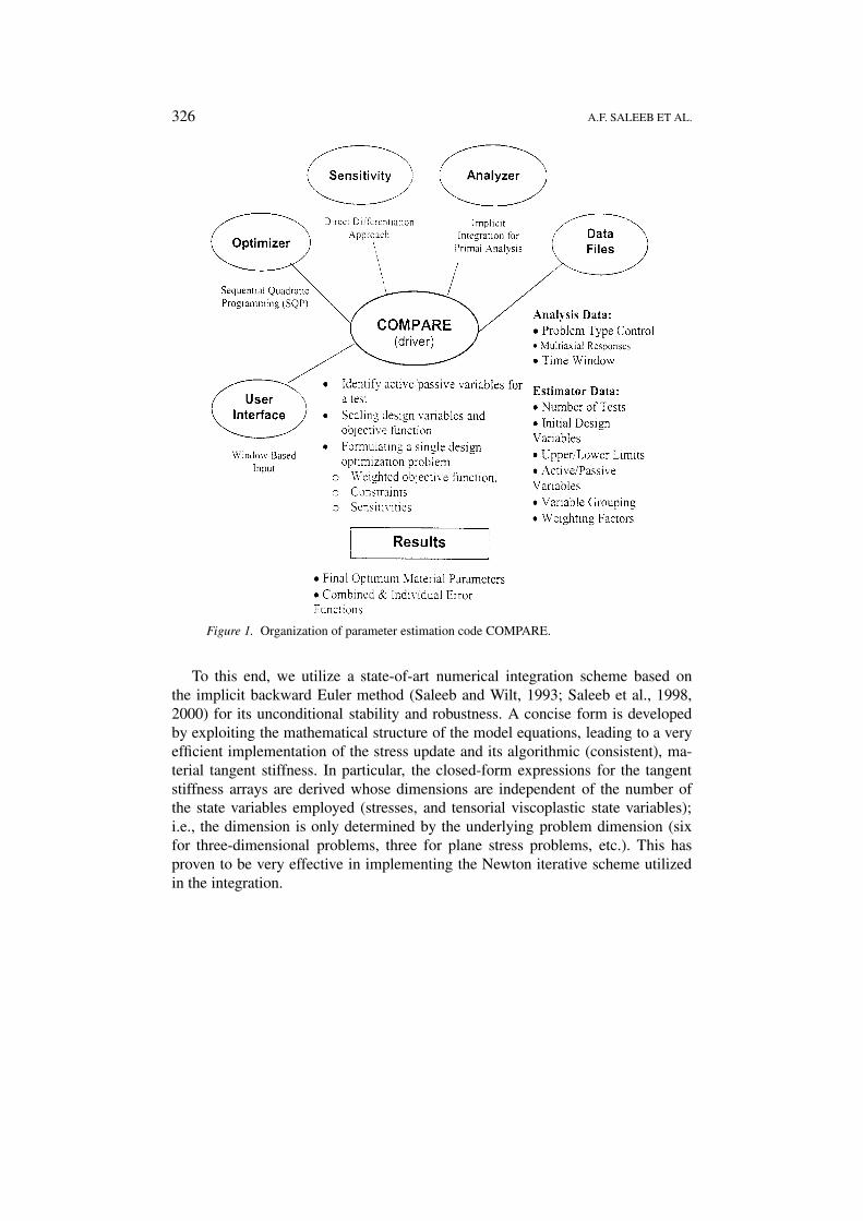
The organization of the modules that form COMPARE is depicted in Figure 1. Thecentral processor in COMPARE links these four modules to formulate the estima-tion of the material parameters as a minimum-error (weighted multi-objective) op-timization problem, and then solves it using the sequential quadratic programmingtechnique.

2.1. PRIMAL ANALYSIS

The primal analysis module in COMPARE is responsible for simulating the mater-ial response under the various loading conditions present in the experimental tests.This module takes the form of a small nonlinear finite element code built upon asingle, element for plane stress analysis. A finite element solution scheme has beenchosen to provide flexibility for adding new material models. It also allows suffi-cient generality in handling different control modes (stress/strain/mixed) under multi-axial (two-dimensional) stress conditions, but still utilizing aunified, strain-driven format for the implementation of the stress update algorithm.The primal analysis module has been written to be as numerically robust as pos-sible.


Figure 1. Organization of parameter estimation code COMPARE.

To this end, we utilize a state-of-art numerical integration scheme based onthe implicit backward Euler method (Saleeb and Wilt, 1993; Saleeb et al., 1998,2000) for its unconditional stability and robustness. A concise form is developedby exploiting the mathematical structure of the model equations, leading to a veryefficient implementation of the stress update and its algorithmic (consistent), ma-terial tangent stiffness. In particular, the closed-form expressions for the tangentstiffness arrays are derived whose dimensions are independent of the number ofthe state variables employed (stresses, and tensorial viscoplastic state variables);i.e., the dimension is only determined by the underlying problem dimension (sixfor three-dimensional problems, three for plane stress problems, etc.). This hasproven to be very effective in implementing the Newton iterative scheme utilizedin the integration.


2.2. SENSITIVITY ANALYSIS

Regarding the second module of COMPARE, methods and algorithmic details dif-fer for evaluating the sensitivity analysis (Adelmann and Haftka, 1986; Vidal andHaber, 1993). Among many others, the most common approaches for sensitivitycalculations can be listed as: (a) the finite difference methods (FDM); (b) the evol-utionary sensitivities approach (ESA); (c) the adjoint sensitivity approach (ASA),and (d) the direct differentiation approach (DDA). The methods in (a) are knownto be prohibitively time expensive and are prone to truncation and/or round-offerror. The second (ESA) approach (e.g., Senseny et al., 1993) requires a ratherspecialized set of coding techniques, far exceeding in their complexity the demandsof the primal analysis part. That is, it calls for the interchange of the order indifferentiations, with respect to time and material parameters, of the raw formsof evolution and flow rate equations of the model. This leads to a separate setof coupled nonlinear first order differential equations for the sensitivities of theresponse (e.g., the stress) and all internal variables (in an experiment under uniaxialstrain control) with respect to each and every material parameter involved in themodel. On their own, these new sets of differential sensitivity equations, with theirexceedingly large number (e.g. even for a uniaxial model containing 10 materialparameters and three state variables such as stress, drag stress, and back stress, thisnumber totals 3×10 = 30) are typically very stiff, thus requiring quite an elaborate(usually high order) time integration scheme to maintain stability and accuracy andto cope with potential singularity problems.

On the other hand, because of their regressive/convolution nature of computa-tion, and the corresponding large storage requirements, the third ASA methods areknown (e.g., Vidal and Haber, 1993) to be only efficient when the response func-tionals are significantly less in their number compared to the number of design vari-ables (i.e., the material parameters in our case). Considering the present situationwith viscoplasticity; i.e., for coupled, transient, history-dependent, responses thesituation is completely opposite, thus rendering the ASA approach less appealing.

Finally, with regard to the DDA approach, these explicit sensitivity methodsare known to be very efficient since they only require a small fraction of the ori-ginal primal-analysis cost. However, this is achieved at the expense of laboriousderivations that must be made in direct linkage with the particular primal-analysisproblem being solved. Herein, we utilized the DDA method, for its efficiency, toderive ‘explicit’ expressions for the response sensitivities under different controlmodes. With this, the sensitivities arrays are evaluated only once after convergenceof the primal analysis phase.

2.3. NONLINEAR OPTIMIZATION

As far as the optimization technique is concerned, COMPARE formulates amulti-objective optimization problem and solves it using a Sequential Nonlin-ear Programming technique. At present, this is known to be one of the best


available, gradient-based, nonlinear optimization techniques. Several features havealso been incorporated into COMPARE to facilitate the estimation of the ma-terial parameters. These include the following: (i) design variable formulationwhich includes variable grouping, i.e., active/passive variables, (ii) constraint for-mulation including variable bounds, (iii) general scaling of variables as well asobjective functions; (iv) formulating a single optimization problem through theweighted-multi-objective function methodology, and (v) the use of quasi-Newtonand line search techniques for solution enhancements. In brief, the estimator toolis of the optimal strategy type, in which the nonlinear mathematical program-ming problem is solved utilizing a successive quadratic programming technique(Powell, 1977; Schittkowski, 1980, 1983, 1986; Leunberger, 1984). Such an op-timization technique is based on an iterative formulation and solution of severalquadratic-programming sub-problems. Each sub-problem may be obtained utiliz-ing a quadratic approximation of the system Lagrangian and a linearization of theconstraints at each iteration.

Finally, a graphical user interface, GUI, has been written for COMPARE inorder to facilitate the data entry task of the users. It is written in the Tcl/Tk scriptinglanguage (Welch, 1997) for better portability to different machines. Such a userinterface internally constructs all of the required files for COMPARE to execute,eliminates much of the tedious data preparation, and allows post-processing of theresults for comparing the experimental data to the model predictions to assess thequality of the fits.

3. Viscoplastic Material Models

A specific class of models, which is representative of the present state-of-art inmetal viscoplasticity (of the generalized J2 or von Mises type), is considered here.For brevity, this will be referred to as GVIPS model (for Generalized VIsco-plasticity with Potential Structure). The model includes a number of distinctivefeatures, and collectively spans a very wide spectrum of characteristic and predict-ive capabilities that are shared by many other viscoplastic models. For example,the formulation (Arnold and Saleeb, 1994; Arnold et al., 1995; Saleeb and Wilt,1993; Saleeb et al., 1998, 2000) is unique in its utilization of a nonlinear kinematichardening (back stress) mechanism resulting from an assumed thermo-dynamicpotential (Gibb’s) function for the ‘equation-of-state’ defining the associated (con-jugate/dual) internal strain variable, as well as a dissipation function, including athermal (static) recovery contribution, for its rate of revolution. A characteristicpartitioning, with several regions of discontinuities of the state (stress-internalvariable) space is also used to account for stress-reversal/cyclic loading. For theflow equations, simple power functions are typically employed. The GVIPS modelis very appealing in view of its theoretically sound basis from the thermodynam-ics standpoint, and the symmetries exhibited in the corresponding linearization ofthe integrated forms of its flow and evolution equations. A summary of the main


equations of this class of material models is outlined in the following subsections(for more details, please see Arnold and Saleeb, 1994; Arnold et al., 1995; Saleeband Wilt, 1993; Saleeb et al., 1998, 2000). In addition, a transversely isotropicelastic-viscoplastic material, i.e., a solid reinforced by a single family of fibers asin Robinson and Duffy (1990), Robinson et al. (1987), Saleeb and Wilt (1993) andKojic and Bathe (1987), is assumed. All derivations are restricted to the case ofsmall deformations and isothermal conditions. For convenience, we utilize bothindex and matrix notations interchangeably.

3.1. ELASTIC RESPONSE

The hyper-elastic response is assumed to be linear. That is, a quadratic strain-energy-density function, �e, is assumed to exist such that the Cauchy (true) stresscomponents are given by

σij = ∂�e

∂εeij= Ce

ijklεekl, (1)

where a superscript ‘e’ denotes the elastic component, and the expression

εij = εeij + εiij (2)

holds true in accordance with the basic hypothesis of the additive decompositionof the total strain tensor, εij , into elastic, εeij , and inelastic components, εiij . In theabove, Ce

ijkl denotes the fourth-order symmetric elastic moduli tensor; see Saleeband Wilt (1993) for its details in case of isotropy (i.e., two elastic moduli, E and ν,for Young’s modulus and Poisson’s ratio, respectively) and anisotropy (e.g., withfive elastic constants for transverse anisotropy).

3.2. THE VISCOPLASTIC RESPONSE

For the viscoplastic response, the plastic dissipation function, �, is written in termsof the ‘anisotropic’ invariants of the stress tensor, σij , the internal tensor variable(back stress) αij and the material anisotropy direction tensor, Vij , (e.g. used fordefining a single family of fibers as in a reinforced composite) including separateflow/hardening and static-recovery contributions, �1 and �2, respectively,

� = �(σij , αij , Vij ) = �1(σij , αij , Vij )+�2(αij , Vij ), (3)

� = �1(F )+�2(G), (4)

ε̇iij = ∂�

∂σij= ∂�1

∂σij, (5)

γ̇ij = − ∂�

∂αij, (6)


and the material directionality Vij is defined as Vij = vivj , where v is the unitvector defining the material fiber direction.

The F and G are scalar quadratic functions in terms of the invariants of thedeviatoric components of the effective stress, (σij − αij ), and the back stress, αij ,tensors, respectively, and are defined as,

F = 1

2k2T

(σij − αij )Mijkl(σkl − αkl)− 1 (7)

and

G = 1

2k2T

(αij )Mijkl(αkl) (8)

with Mijkl denoting a symmetric fourth-order tensor which is a function of thematerial fiber orientation tensor Vij defined as

Mijkl = Pijkl − ξQijkl − 1

2ζRijkl . (9)

In Equation (9), 0 ≤ ξ ≤ 1 and 0 ≤ ζ ≤ 1 are material parameters defining thestrength ratios, i.e.,

ξ = η2 − 1

η2, ζ = 4(ω2 − 1)

4ω2 − 1,

η = k!

kT, ω = Y!

YT, (10)

where the constants kT (and k!) and YT (and Y!) are threshold strengths of thecomposite material in transverse (and longitudinal) shear and tension/compression,respectively. The fourth-order tensors Pijkl , Qijkl and Rijkl are defined as (e.g.,Saleeb and Wilt, 1993)

Pijkl = Iijkl − 1

3δij δkl, Iijkl = 1

2(δikδjl + δilδjk),

Qijkl = 1

2(Vikδjl + Vilδjk + Vjlδik)− 2VijVkl,

Rijkl = 3VijVkl − (Vij δkl + Vklδij )+ 1

3δij δkl . (11)

For the isotropic case, ξ = ζ = 0 and Mijkl reduces to Pijkl , i.e., the classicalvon-Mises-type forms in function F and G.

For the case considered here, the present purely mechanical theory has thefollowing decoupled form of Gibb’s complementary free-energy density functionin terms of stress and internal state parameters, i.e., with superscripts ‘e’ and ‘i’indicating elastic and inelastic parts,

�(σij , αij ) = �e(σij )+�i(αij ). (12)


The terms �e and �i are defined to have the following forms

�e(σij ) = 1

2σij (C

eijkl)

−1σkl,1

k2T

∂�i

∂G= 1

h,

h = H

Gβ(power-law hardening), or

= H(1 −Gβ/2) (saturation hardening), (13)

where H and kT (stress units), and β (dimensionless) are (positive) material con-stants. The function G was defined previously in Equation (8). Together with thestrain vector decomposition of Equation (2), the above equations (12) and (13)define the equations of state,

εij − εiij = ∂�e

∂σij= (Ce

ijkl)−1σkl,

γij = ∂�i

∂αij= 1

hπij , (14)

in which πij is defined as

πij = Mijklαkl. (15)

We also define the free energy �̄(εe, γ ) through the ordinary Legendre-type

transformation, i.e., �̄ = �̄e + �̄i , where �̄e = �e for linear elasticity, and�̄i = α · γ − �i(α). The dissipation function �(σij , αij ) is now introduced as

� = σij ε̇ij − ˙̄� ≥ 0. (16)

Substituting for �̇ in terms of σ̇ij and α̇ij from Equations (12–14), one obtains

∂�

∂σij= ε̇iij ,

∂�

∂αij= −γ̇ij = −

(∂2�i

∂αij ∂αkl

)α̇kl (17)

The above rate form connects α̇ij and γ̇ij through the hardening-moduli tensorwhich is the Hessian matrix of �i . Using Equation (17) and the second ofEquation (13), yields

α̇ij = h

[Zmijkl +

h′

h(1 − h′h(2k2

T G))αijαkl

]γ̇kl = [Lijkl]−1γ̇kl, (18)

where Lijkl is the present, single, compliance operator (e.g., Arnold and Saleeb,1994; Arnold et al., 1995; Saleeb and Wilt, 1993), and h′ is a scaled derivative

h′ = 1

k2T

dh

dG. (19)


In addition, Zmijkl above is defined as the ‘generalized inverse’ of the deviatoric,

positive semi-definite, material tensor operator Mijkl , i.e.,Zmijkl = M−1

ijkl (see Saleeband Wilt, 1993, for details of this ‘inverse’ under different conditions; e.g., three-dimensional, plane strain/axisymmetric, generalized plane stress, etc.).

From Equations (13) and (17), the final expressions for the inelastic flow andevolution equations for the specific selection of power functional forms for �1(F )

and �2(G), Equation (4) can be straightforwardly derived; i.e.,

ε̇iij = f (F ).ij , .ij = Mijkl(σkl − αkl), (20)

γ̇ij = ε̇iij − λ

hπij , πij = Mijklαkl, (21)

α̇ij = [Lijkl]−1

(ε̇ikl −

λ

hπkl

), (22)

where f , h, and λ are the flow, hardening, and recovery functions (all of nonlinearpower functional form), respectively, which are defined as

f (F ) = Fn

2µ, h = H

G+G0)β(power),

h = H(1 −Gβ/2) (saturation), λ = RGm−β, (23)

in which n, µ, H , β, R and m are (positive) material constants.Several regions of discontinuities in the state space are introduced to account

for stress-reversal/cyclic-loading/dynamic-recovery effects. This simply amountsto using different functional forms for f and h in different regions, i.e.,

f = f if F > 0,

f = 0 otherwise; (24)

h = h if (σij − αij )πij > 0,

h = H (saturation)

= H

Gβ

0

(power) otherwise; (25)

The ‘small’ constant (cut-off value) G0 is an ‘adjusted’ parameter (selected here tobe 10−5) to prevent singularity in h (see the second of Equation (23)) whenG → 0.

Finally, a number of important remarks are in order regarding the above math-ematical formulation. Firstly, we emphasize that the model is based upon a purelyphenomenological approach, i.e. for macroscopic-level descriptions (as opposed tothe more fundamental microscopic approach). Secondly, the details of the model


were largely motivated by consideration of the underlying physics of metal de-formations; i.e. originated in the dislocation theories; e.g. see Saleeb et al. (2001).Indeed, this is also the rational behind the choice of the representative (power-type)functional forms selected above.

On the other hand, it is presently well recognized that, despite the marked dif-ferences in the underlying physics on the microscale, different classes of materialsystems (e.g. metals, polymer-based composites, etc.) do exhibit qualitatively sim-ilar phenomenological manifestations in their measured reponses during testing;e.g. see Chaboche (1997). In fact, it is with this premise that we proceeded withthe latter applications to various types of materials. For example, considering therather extreme specialization to viscoelasticity (e.g. predominate in polymer com-posites) from the basically viscoplastic forms above (e.g. significant in metals).This can be obtained as follows; i.e., with exponents n = m = β = 0 in Equa-tion (23), the model reduces to (essentially) linear viscoelasticity when the plasticthreshold, kT in Equation (7), is discarded. Furthermore, with a significant valueof the static/thermal recovery term R (relative to H in Equation (23)), it is thenpossible to allow complete recovery of strains (upon unloading and holding at zerostresses) as typical with three-elements solids in viscoelasticity. Further extensionsallowing a wide spectrum of viscoelastic relaxation times are also possible throughthe use of multiple internal (kinemtaic-hardening) stress components α; see Saleebet al. (2001) for further details, and also some of the applications in Section 6.

3.3. ALGORITHMS FOR STRESS UPDATE AND CONSISTENT TANGENT

STIFFNESS

The fully implicit backward Euler integration scheme is presented in this section.The derivation of the equations follow a systematic process outlined below. Inparticular, we utilize a strain-driven format for the time marching strategy fromthe known state at time tn to the targeted (unknown) state at time tn+1 over onetypical time increment 4t = tn+1 − tn. The first step is to write the local updateexpressions for the stress and internal variables, i.e.,

σ n+1 = σ n +4σn+1, (26)

αn+1 = αn +4αn+1. (27)

Using the implicit update equation, i.e., Equations (26) and (27), construct theupdate expressions for the stress, σ and internal state variable, α. That is, withgiven 4ε = εn+1 − εn, and making use of Equations (18) and (20)-(22),

σ n+1 = σ n + Ce(4ε −4tf .n+1), (28)

αn+1 = αn +4t

[Zm + h′

h(1 − h′h(2k2

T G))(α ⊗ α)

](hf. − γ π)|n+1. (29)


The second step involves forming residual vectors, which are necessary parts of theiterative implicit scheme. Thus, using Equations (28) and (29), the residual vectorsmay be defined as

Rσ = σn+1 − [σ n + Ce(4ε −4tf .)|n+1], (30)

Rα =(M −

(h′

hπ ⊗ π

)∣∣∣∣n+1

)(αn+1 − αn)−4t(hf. − λπ)|n+1. (31)

Referring to Equations (26) and (27) the ultimate objective is to calculate the in-crements in stress and the internal variables. Thus, consider the first-order Taylorseries expansion of the residual vectors, i.e.,

Rk+1σ = Rk

σ + ∂Rσ

∂σ

∣∣∣∣k

dσ k + ∂Rσ

∂α

∣∣∣∣k

dαk, (32)

Rk+1α = Rk

α + ∂Rα

∂σ

∣∣∣∣k

dσ k + ∂Rα

∂α

∣∣∣∣k

dαk. (33)

Note that the subscript n+1 is dropped for clarity, and the index ‘k’ is the iterationcounter.

The third and final step is to form the necessary iterative corrections in stressand internal variables, dσ and dα using Equations (30–33). During the derivations,an objective is to factor and group the expressions in terms of the stress incrementdσ kn+1. This leads to

dσ kn+1 = −J−1(Ce−1Rσ + P 4P−11 Rα), (34)

dαkn+1 = −P−11 (Rα − P 2 dσ kn+1). (35)

Note that, in the above equations, the dimensions of the vectors and matrices areof the order of the underlying physical stress-space dimension. That is, for a three-dimensional space, and accounting for the second-order tensors dσ and dα, thevectors are 6 × 1 and the matrices are 6 × 6. Thus the size has been reduced froma possible 12 × 12 matrix size to a maximum dimension of 6 × 6 for all arraysinvolved.

Now Equations (34) and (35) along with the iterative form of the updateequations, i.e.,

σ k+1n+1 = σ kn+1 + dσ kn+1, (36)

αk+1n+1 = αkn+1 + dαkn+1, (37)

constitutes the complete, fully implicit integration algorithm. In Equation (34), Jis the iteration Jacobian matrix,

J = P 3 − P 4P−11 P 2 = Ce−1 + P 4(I − P−1

1 P 2) (38)


with the following additional matrices defined:

P 1 = Z−1m + P 2 +4tλM +

[4tλ′ − h′

h(4tλ+ 1)

](π ⊗ π)

+ ρ

[(h′

h

)2

− h′′

h

](π ⊗ π)

− ρ

(h′

h

)2 [M −

(h′

h

)(π ⊗ π)

]

−(h′

h

)[(πn+1 − πn)⊗ πn+1 + (πn+1 − πn)⊗ πn+1], (39)

P 2 = hP 4, P 4 = 4t(fM + f ′. ⊗ .) (40)

P 3 = Ce−1 +4t(fM + f ′. ⊗ .) = Ce−1 + P 4. (41)

In the above, the primes indicate ‘scaled’ derivatives as given below:

f ′ = 1

k2T

df

dF, h′ = 1

k2T

dh

dG, λ′ = 1

k2T

dλ

dG, h′′ = 1

k2T

dh′dG (42)

and the scalar is defined as

ρ = πTn+1 · (αn+1 − αn). (43)

Note that all arrays and functions in Equations (38) to (43) are evaluated based onthe last updated state (σ kn+1, αkn+1), unless indicated otherwise. Note also that thestate (σ n, αn) corresponds to the converged global solution at the last time step;i.e., they are kept constant during the local iteration sequence in Equations (36)and (37).

In keeping with the underlying fully implicit integration scheme, one canstraightforwardly proceed to differentiate the updated stress field, σkn+1 to obtainthe algorithmic (also consistent) viscoplastic-moduli or material tangent stiffnessmatrix, Cev, for use in the finite element stiffness calculations. The derivations willin fact lead to

Cev = J−1 = [Ce−1 + P 4 − hP 4P−11 P 4]−1, (44)

Clearly, Ce and P 1, P 2, P 3, and P 4 are symmetric, resulting in a symmetric tangentstiffness Cev.

4. Explicit Material Parameter Sensitivities

Following a direct-differentiation (DD) approach, the ‘exact’ expressions for thematerial parameter sensitivities are naturally derived and utilized for the sensitivity


calculations. Simply stated, these sensitivities will provide the necessary arraysgiving the extent by which a calculated response component (for example, totalstrain in a stress-controlled conventional creep test) will change as a result of (unit)changes in material parameters. Because of the time variant nature of the exper-imental tests (creep, relaxation, etc.) these latter arrays are naturally provided astime histories. Such an approach is computationally efficient in that the sensitivityexpressions are only calculated once after the primal analysis phase. The generalperceived disadvantage of this technique is, however, the necessary analytical de-rivation of the sensitivities. While such derivations may be complicated, the benefitin terms of computational efficiency and elimination of the drawbacks associatedwith the other competing approaches are believed to be worth such effort (e.g., seeSection 2.2). The key to the closed form gradient generation lies in the fact thatthe stress function of the viscoplastic material model is expressed in terms of thematerial parameters. Such material parameters can be expressed in a vector formX as (e.g., without elasticity and anisotropy material parameters, for brevity)

X = [kT , n, µ,m, β,R,H ]T . (45)

Sensitivity calculations, of course, depends on the type of control utilized inthe experimental test; e.g., stress-, strain-, or mixed-controls. For conciseness, weconsider below the case of strain control in detail. The final forms for the stress andmixed controls are also provided. It can be noticed that the general case of mixedcontrol is simply obtained from the results of the two other cases by a ‘careful’partitioning.

4.1. MATERIAL PARAMETER SENSITIVITY FOR A STRAIN-CONTROLLED

TEST

In this case, the material parameter sensitivity functions become the measuredtime-history of stresses. Their sensitivities with respect to the material parametersare simply obtained from the appropriate derivatives of the integrated (algorithmic)stress and state variable fields, i.e., Equations (30) to (31), with zero residualvectors Rσ and Rα , Equations (36) and (37), which occur after convergence. Inthis, two major contributions are obtained: (i) from the explicit dependence ofthe integrated stress/state variables on material parameters; (ii) from their implicitdependence through the history of sensitivity at state (n) and the correspondingsensitivity changes because of dependence of Rσ on the converged σn+1 andαn+1 values. Thus, one speaks of the evolution-in-time of the sensitivity arrays,(Dσ/DX)(t) and (Dα/DX)(t), at different instants of time (t).

For the present case of strain control (specified εn+1 and εn), we can then showthat the final expressions for sensitivity matrices are given by(

Dσ

DX

)n+1

= J−1

[Ce−1

[−

(∂Rσ

∂X

)exp

+(Dσ

DX

)n

]


− P 4P−11

[(∂Rα

∂X

)exp

−Q∗(Dα

DX

)n

]], (46)

(Dα

DX

)n+1

= P−11

[P 2

(Dσ

DX

)n+1

−(∂Rα

∂X

)exp

−Q∗(Dα

DX

)n

], (47)

where (.)exp indicates explicit derivatives of (.), which can be expressed as (e.g. inthe case of power hardening)(

∂Rσ

∂X

)exp

= Ce.

[−2n

µkTFn−1(F + 1),

1

µFn lnF,−F

n

µ2, 0, 0, 0, 0

]4t,(48)

(∂Rα

∂X

)exp

= (. 9+ π S)4t, (49)

where

9 =[(

nh

µkTFn−1(F + 1)− βH

µkTGBFn

),−h2µ

Fn lnF,hFn

2µ2, 0,

H

GB

Fn

2µlnG, 0,

−Fn

2µGB

], (50)

S =[−2RmGm

kT, 0, 0, RGm lnG, 0,Gm, 0

], (51)

with Q∗ denoting the ‘inverse’ of tensor Lijkl in Equation (18); i.e.,

Q∗ = 1

h

[M − h′

hπ ⊗ π

], (52)

which is a symmetric matrix.It can be noted that all the arrays in the above sensitivity expressions have been

defined previously in the integration scheme; i.e., no extra computational cost isrequired here. Consequently, the entire calculations for sensitivity arrays simplyreduces to a recursive (noniterative) evolution; i.e., from their stored values attime station tn directly to the new station at tn+1; e.g., as per the prescription ofEquations (46) and (47).

4.2. MATERIAL PARAMETER SENSITIVITY FOR A STRESS-CONTROLLED

TEST

For stress control (i.e., specified σn and σn+1), one can arrive at the sensitivitiesfor strains and internal state variables as(

Dε

DX

)n+1

=(Dε

DX

)n

+{Ce−1

(∂Rσ

∂X

)exp


− P 4P−11

[(∂Rα

∂X

)exp

−Q∗(Dα

DX

)n

]}, (53)

(Dα

DX

)n+1

= −P−11

[(∂Rα

∂X

)exp

−Q∗(Dα

DX

)n

]. (54)

4.3. MATERIAL PARAMETER SENSITIVITY FOR A MIXED-CONTROLLED

TEST

For mixed control, a part σ (1) of the stress of order M and a part ε(2) of the strain oforder N are responses for the imposed remaining parts σ (2) and σ (1), respectively,where partitions (1) and (2) are naturally orthogonal and the sum of N +M givesthe total dimension of the physical stress space (e.g., six in the three-dimensionalproblem). The inverse of the elastic moduli tensor and J -matrix can be partitionedas

Ce−1 =[Ce−1

11(M×M)Ce−1

12(M×N)Ce−1

21(N×M)Ce−1

22(N×N)

], J =

[J e−1

11(M×M)J e−1

12(M×N)J e−1

21(N×M)J e−1

22(N×N)

], (55)

where the submatrix Ce−1

11 is of order (M ×M), Ce−1

22 is of order (N ×N), and Ce−1

12is an (M × N). The sensitivities arrays for stresses, strains, and internal variablescan be expressed as(

Dσ(1)

DX

)n+1

= J e−1

[(a(1) + b(1))+ Ce−1

11

(Dσ(1)

DX

)n

], (56)

(Dε(2)

DX

)n+1

=(Dε(2)

DX

)n

+ J e−1

21

(Dσ(1)

DX

)n+1

− (α(1) + b(1))− Ce−1(Dσ(1)

DX

)n

, (57)

a =[a(1)

a(2)

]= −Ce−1

(∂Rσ

∂X

)exp

, (58)

b =[b(1)

b(2)

]= −P 4P

−11

[(∂Rα

∂X

)exp

−Q∗(Dα

DX

)n

]. (59)

5. Optimization Algorithm

As alluded to previously (Section 2.3), the optimization scheme in COMPAREformulates a multi-objective optimization problem from information specified


in data files, for both experimental measurements and simulated responses, andthen solves it by using a sequential quadratic nonlinear programming technique(Schittkowski, 1980, 1986, 1988). To this end, we cast the optimal materialparameters as the following nonlinear mathematical programming problem:

find the n variables in X within prescribed upper and lower bounds (i.e.,XLi ≤ Xi ≤ XU

i , i = 1, 2, . . . , n) to minimize the weighted function �(X)under a set of inequality constraints ng.

In the above, X represents the independent, active, variables for viscoplasticmaterial; e.g., see Equation (45).

The multi-objective weighted function for a number of mt response measure-ments (i.e., mt experimental test data) can be expressed in terms of the following‘error norms’

�(X) =mt∑i=1

Wi

fi(X)

|fi0(X)|, (60)

where

fi(X) = 1

2

nm∑j=1

nR∑k=1

(1 − Rn

Rkm

)2

. (61)

In the above, Wi is the weighted parameter for the ith test (∑mt

i=1 Wi = 1); fi(X)is the objective function for the ith test; fi0(X) is the initial value of the objectivefunction for the ith test; nm is the number of measurement stations along the spe-cified load history in a given test; Rk and Rkm are the kth stress/strain componentsfrom the analysis and test data, respectively; and nR is the number of stress/straincomponents at a particular time; i.e., j th station.

Utilizing a successive quadratic programming technique to solve the nonlinearprogramming problem simply amount to the following formal statements (Powell,1977), where ng is the number of (nonlinear) constraints

minX∈Rn

�(X) (62)

subject to

g!(X) > 0 for ! = 1, 2, . . . , ng, (63)

XL ≤ X ≤ XU. (64)

Such an optimization technique is based on iterative formulation and solution ofquadratic programming sub-problems that can be obtained by using a quadraticapproximation of the system’s Lagrangian and linearizing of the constraints at thekth iteration as

mind∈Rn

1

2dTk H kdk + ∇�(X)T dk (65)


subject to

∇g!(X)T dk + g!(X) ≥ 0, ! = 1, 2, . . . , ng (66)

XL −Xk ≤ dk ≤ XU −Xk, (67)

where dk is the solution of the sub-problem; Hk is the positive definite approxim-ation of the Hessian matrix; Xk is the variables at the kth iteration; ∇�(X) is thegradient of the weighted objective function; and ∇g!(X) is the gradient of the !thconstraint.

A line search scheme is then used to fined a new variable Xk+1,

Xk+1 = Xk + αdk, α ∈ (0, 1], (68)

such that the objective function �(Xk+1) has a lower value at the new state variableXk+1.

COMPARE contains a capability for obtaining the material parameters of theviscoplastic model directly from test data. It is recommended to obtain the mater-ial parameters from several experiments involving different kinds of deformationsover a range of stress/strains, rates, and times of interest in the actual applications.This is particularly significant in view of the fact that parameter identification prob-lems are known to be prone to severe nonuniqueness/instability problems unlessthe experimental data are sufficiently ‘rich’ in their contents so as to activate allinvolved parameters (and mechanisms) in the model.

Once the viscoplastic material constants are determined by COMPARE, thequality of the model’s correlation with the test data can be assessed. This is simplydone by using the plotting capability in COMPARE to graphically show how wellthe model’s prediction of the material behavior, under different deformation modes,compares with the experimental data. At this point, the user has to judge whetherthe material parameters determined by COMPARE are acceptable.

Finally, an important remark is in order with regard to the actual implementationof the scheme summarized in Equations (60) to (68). In all these equations thetreatment proceeds with scaled sets of variables; i.e., X(scaled)

i = Xi/X(0)i , where

X(0)i is the starting value of the ith design variable (optimization iteration number

zero). Similar definitions for bounds on variables, subsequent sensitivities, etc. areconsidered. Together with the implied scaling in Equations (60) and (61), whichalleviates the difficulty with ‘dimensionality’ in dealing with different tests (e.g.with one test measuring stress response, as in relaxation or constant-strain-ratetensile test and another measuring strains, as in creep experiments), the use ofX(scaled) was found to be crucial for the accuracy and convergence properties of thealgorithms.


6. Numerical Simulations and Characterization

The primary objective of this section is of three-fold: (i) to assess the accuracyof the derived expressions for the sensitivities as well as the developed meth-odology for optimization for different classes of tests (i.e., stress-, strain-, ormixed-controls); (ii) to actually characterize the material parameters under iso-thermal conditions and using the isotropic form of the viscoplastic model GVIPS,given comprehensive experimental data for TIMETAL 21S (which is the re-gistered trademark of TIMET, Titanium Metals Corporation), and (iii) to providea new anisotropic characterization for composite material system; i.e. W/Kanthaland AS4/PEEK with bi-axial strain measurements, and (iv) to report results oncharacterization of IN738LC under cyclic multiaxial loading.

In the following applications, all of the elastic material parameters are assumedknown and are made ‘passive’ during the optimization process. Note that ‘passive’signifies that the specified material parameters are held fixed at their initial inputvalues during the optimization process. On the other hand, ‘active’ signifies mater-ial parameters that are free to move between bounds (upper and lower) during theoptimization process. With this in mind, the current viscoplastic model requires atotal of seven material parameters that need to be determined. Three of these areassociated with the flow law; i.e., kT , µ and n; two with the nonlinear hardeningoperator; i.e., H and β; and two with the internal thermal recovery term; i.e., Rand m. Inasmuchas COMPARE conducts a least square, constrained, nonlinearoptimization problem, the primary task of the user is the selection of appropriateupper and lower bounds as well as initial values for all material parameters. Notethat the need for judicious selection of these bounds and the initial values is notdriven by numerics (as COMPARE has been shown to be extremely robust andcomputationally efficient) as much as by the physics of the problem.

6.1. VALIDATION TESTS

The optimization methodology developed in COMPARE has been assessedthrough: (i) comparing the direct (explicit) sensitivities derived with those obtainedby the conventional finite difference scheme; (ii) simulating ‘measured’ data bythe GVIPS model for a fixed set of material parameters, for different types oftests, and then using the optimization scheme to predict the material parametersutilizing different initial values for these parameters. To this end, one tensile testat a strain rate of 0.108/sec, three conventional creep tests at constant stresses of10, 20 and 30 Ksi, and one relaxation test at a constant strain of 10−3 are utilized.In all these simulations, the Young’s modulus and Poisson’s ratio are considered tobe equal to 30000 Ksi, and 0.3, respectively; and the seven material parameters forthe viscoplastic response are given in Table I.


Table I. Viscoplastic material parametersfor validation test.

Parameter Unit Value

kT Ksi 0.6823

n – 1.5

µ Ksi.sec 25000

m 00 1.5

β – 1.5

R 1/sec 5.556 × 10−10

H Ksi 18000

Table II. Material parameter sensitivities for the tensile test.

Material Time step number 1 Time step number 25 Time step number 50

parameters Explicit Finite Explicit Finite Explicit Finitedifference difference difference

kT 16.0340 16.0321 24.1918 24.1992 26.2758 26.2731

n –12.8053 –12.7862 –14.0278 –14.0052 –14.0326 –14.0103

µ 1.1632E-4 1.1627E-4 1.2534E-4 1.2529E-4 1.2538E-4 1.2533E-4

m –5.2902E-11 –6.0396E-11 –5.1621E-7 –5.1765E-7 –2.4249E-6 –2.4323E-6

β –1.4486 –1.449 –9.1001 –9.0866 –11.9538 –11.9352

R –6.8245 –6.7141 –250.445 –250.450 –1071.526 –1071.524

H 3.9068E-5 3.9053E-5 1.2960E-4 1.2956E-4 1.5588E-4 1.5583E-4

6.1.1. Explicit versus Finite Difference Sensitivities

The explicit sensitivities have been compared with those derived from the conven-tional finite difference scheme for three different test types; i.e., the tensile test, thecreep test under constant stress of 20 Ksi, and the relaxation test. A step size on theorder of the parameter value times 10−4 is used in the finite difference algorithm.The sensitivities obtained for the entire history of loading are in excellent agree-ment with those reported by the finite difference. The sensitivities (reported herefor the actual, nonscaled, parameters for comparison) for only three different steps;i.e., step numbers 1, 25, and 50, are given Tables II to IV for the three test cases.It is worthy noting that the finite difference sometimes could not capture a smallvalue for sensitivities (predict a zero value instead) as shown in Table III with theparameter m and R. Also note the drastically different magnitudes of the sensitivitycoefficients for various parameters, thus the necessity of the proper scaling in theactual implementation of the algorithms (recall Section 2.3).


Table III. Material parameter sensitivities for the creep test.



kT –1.8419E-6 –1.8380E-6 –2.0896 –2.0854 –2.7084 –2.7030

n 8.8099E-7 8.8233E-7 0.72978 0.73003 75.715 75.720

µ –1.439E-11 –1.437E-11 –7.8764E-6 –7.8716E-6 –8.801E-6 –8.797E-6

m –9.1001E-23 0.00 3.0735E-6 3.0837E-6 1.4427E-5 1.4492E-5

β –5.8559E-8 –5.8540E-8 1.2015 1.2030 1.7716 1.7744

R 6.7072E-14 0.00 1259.452 1259.521 5693.79 5693.83

H –1.5598E-12 –1.5590E-12 –1.5172E-5 –1.5161E-5 –2.1554E-5 –2.15345

Table IV. Material parameter sensitivities for the relaxation test.



kT 1.7899E-1 1.7864E-1 4.5844 4.5816 4.5844 4.5817

n –1.1361E-1 –1.1384E-1 2.1588E-1 2.1525E-1 2.1588E-1 2.1525E-1

µ 1.4583E-6 1.4570E-6 –1.7294E-6 –1.7291E-6 –1.730E-6 –1.729E-6

m 9.2111E-19 0.00 –6.3965E-6 –6.4033E-6 –1.5127E-5 –1.5144E-5

β 4.2054E-3 4.2041E-3 –9.4439E-1 –9.4236E-1 –9.4395E-1 –9.4325E-1

R –9.1043E-9 0.00 –9293.57 –9293.71 –2.1978E-5 –2.1976E-5

H 1.4634E-7 1.4628E-7 3.6125E-5 3.6085E-5 3.6124E-5 3.6084E-5

Although the sensitivities obtained explicitly are almost identical to those byfinite difference, the CPU time required for such calculations are different. Relativeto the CPU time required by the direct scheme, the sensitivity calculations obtainedusing the finite differences required 8.004, 8.235, and 7.931 times as much for thetensile, creep, and relaxation test cases, respectively. This is very good evidence ofthe efficiency of the developed explicit sensitivities, which is to be expected in viewof the fact that most of their ingredients are already available during the integrationprocess.

6.1.2. Re-Identification of Target Parameters Using Simulated Data

Several issues are studied in this section to validate the optimization scheme inCOMPARE. These include uniqueness; full versus partial set parameter estimation,and optimization using several test datasets either of the same type or of differ-


Table V. Partial optimum sets for three different test cases.

Tension test Tension test Three creep tests

Active Initial Optimum Active Initial Optimum Active Initial Optimum

parameter parameter parameter

N 0.50 1.5002 µ 20000 24996.93 m 0.50 1.50

(1.50) (25000) (1.50)

β 0.50 1.4997 H 12000 18002.99 R × 10−10 0.50 5.517

(1.50) (18000) (5.556)

Table VI. Optimum parameter set for tension, creep, and relaxation, simulated, test case.

Parameter Lower bound Initial Upper bound Optimum True

kT 0.400 0.50 4.00 0.6823 0.6823

n 0.500 1.0 4.00 1.5025 1.500

µ 10000.0 20000.0 80000.0 24225.85 25000.0

m 0.500 1.00 5.00 0.9999 1.50

β 0.20 0.50 5.00 1.4914 1.50

R 10−10 0.5 × 10−1 1.0 × 10−6 0.4999 × 10−1 5.55 × 10−10

H 12000.0 16000.0 20000.0 16420.669 18000.0

ent types. In all of these studies, the viscoplastic model GVIPS has been utilizedto generate the so-called ‘experimental data’ using the fixed material parametersgiven earlier in Table I. Note that in the following cases, we will refer to these samefixed material parameters used to generate the fictitious data as the ‘true’ values.We then start the optimization exercise with a different set of initial values for theactive material parameters and see if we are able to, in effect, re-fit the test data andconverge back on the same ‘true’ values.

In the first case, COMPARE has been utilized to re-identify a partial set ofmaterial parameters. In this, some of the parameters are considered to be active,while the rest are specified as passive (fixed at their original ‘optimum’ values).Specifically, only two parameters are considered active and the other five are con-sidered passive. Three test cases are examined: (1) the tensile test with n and βas active parameters; (2) the tensile test with ν and H as active; and (3) the threecreep tests withm andR as active. The re-identified values for the active parametersobtained with COMPARE are shown in Table V together with ‘true’ ones (shownhere between parentheses). Upon comparing the obtained optimum values with the‘true’ values in parentheses, it is evident that COMPARE accurately matches the‘true’ values for the active parameters.


Table VII. Sum of error square for tension, creep, and relaxation (simulated) test case.

Tensile test Creep test Relaxation test Weighted errorfunction

Initial 66363.2 140967.0 55.775 69128.66

Optimum 1.069 × 10−3 1.214 × 10−2 1.979 × 10−10 4.405 × 10−3

A second case consists of three tests (i.e., tensile, creep at fixed stress of 20 Ksi,and relaxation tests) that are considered simultaneously for optimization. All ofthe viscoplastic material parameters are considered as active variables. The initialvalues for the parameters as well as the lower and upper bounds are shown inTable VI. In COMPARE, one has the option to specify different weights for eachtest used in the optimization. This flexibility allows the user to add weight (i.e.significance) to some tests over the others. Here, equal weight factors are usedfor the three tests during optimization. COMPARE has successfully obtained anoptimum set, which is also shown in Table VI along with the ‘true’ values for suchparameters. The response history due to initial, optimum, and true set of parametersare shown in Figure 2 for the tensile, creep, and relaxation tests, respectively.

The sum of the error squares for all the three tests at the starting (initial) andfinal (optimum) parameter sets are shown in Table VII. The weighted error func-tions are in effect a measurement of the error (or difference) between the model’sprediction and corresponding the experimentally measured data for all of the testscombined. In this context, having an initial error function of 69128.66 signifieshow ‘far away’ the initial predictions based upon the starting values were from theactual experimental data. How far away the initial guesses (dashed lines) are is alsoclearly demonstrated in Figure 2. On the other hand, at the optimum solution, theerror function has reduced to 4.405×10−5, i.e. the predicted responses based uponthe optimum values are very close to the experimental data. It is worth noting thata reduction of more than seven orders of magnitude in the error (‘cost’) functionwas obtained which shows the robustness of the optimization scheme to handle ‘faraway’ initial guesses and yet obtain a good final correlation with the test data.

Finally, note that despite the good (both qualitative and quantitative) overallmatch observed in Figure 2, some of the re-identified set of seven parameters didnot exactly match their targeted counterparts (see Table VI). This clearly hintsat a possible ‘nonuniqueness’ problem in view of the rather limited content of‘experimental’ data of three tests used (a single tension, a single creep and asingle relaxation test), whereas the involved parameters (particularly the last four inTable VI for hardening/recovery) are designed to account for a wide range of stresslevels, loading rates, and time scales. For the limited tests utilized, the identificationprocess has somewhat ‘repartitioned’ the balance between recovery (m and R) andhardening (β and H ).


Figure 2. Results using three-simulated-test data.


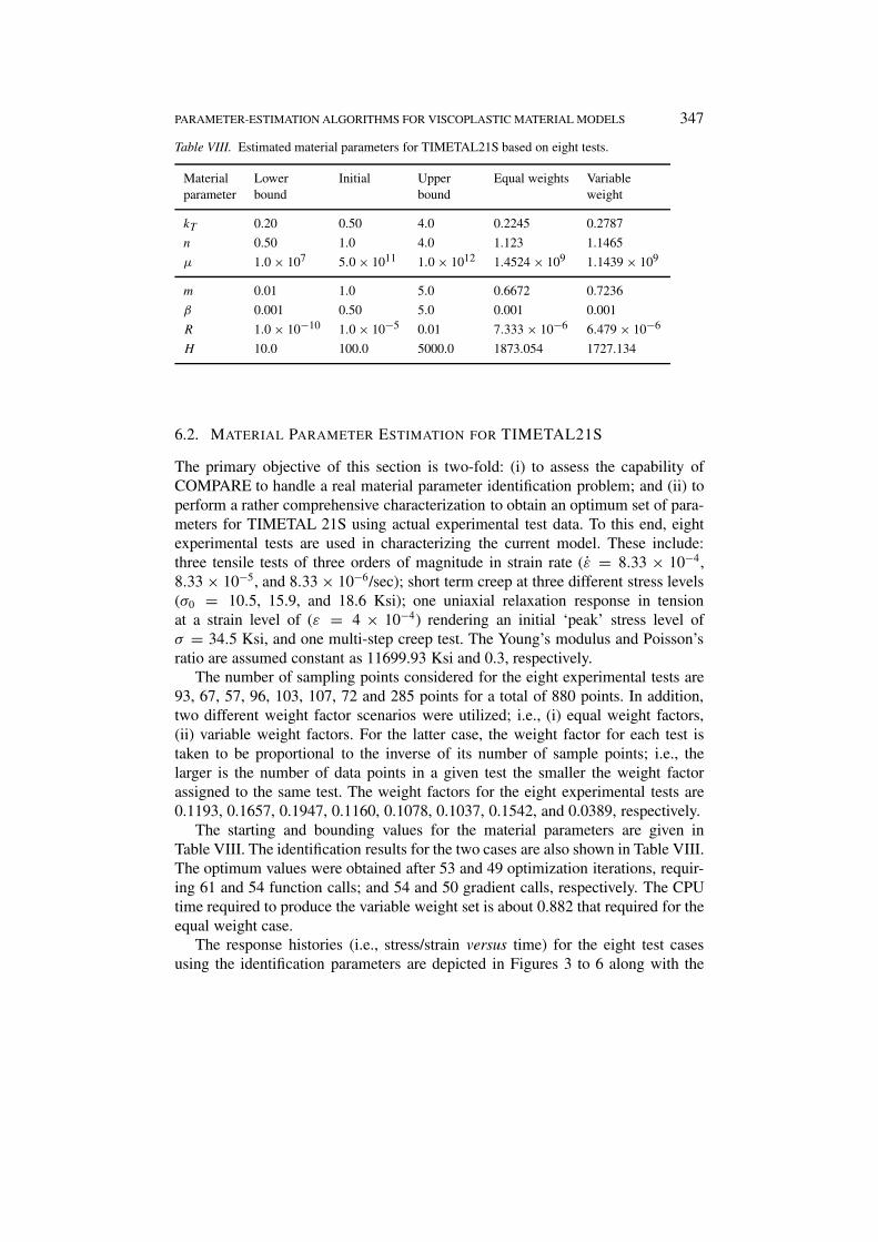
Table VIII. Estimated material parameters for TIMETAL21S based on eight tests.

Material Lower Initial Upper Equal weights Variableparameter bound bound weight

kT 0.20 0.50 4.0 0.2245 0.2787

n 0.50 1.0 4.0 1.123 1.1465

µ 1.0 × 107 5.0 × 1011 1.0 × 1012 1.4524 × 109 1.1439 × 109

m 0.01 1.0 5.0 0.6672 0.7236

β 0.001 0.50 5.0 0.001 0.001

R 1.0 × 10−10 1.0 × 10−5 0.01 7.333 × 10−6 6.479 × 10−6

H 10.0 100.0 5000.0 1873.054 1727.134

6.2. MATERIAL PARAMETER ESTIMATION FOR TIMETAL21S

The primary objective of this section is two-fold: (i) to assess the capability ofCOMPARE to handle a real material parameter identification problem; and (ii) toperform a rather comprehensive characterization to obtain an optimum set of para-meters for TIMETAL 21S using actual experimental test data. To this end, eightexperimental tests are used in characterizing the current model. These include:three tensile tests of three orders of magnitude in strain rate (ε̇ = 8.33 × 10−4,8.33 × 10−5, and 8.33 × 10−6/sec); short term creep at three different stress levels(σ0 = 10.5, 15.9, and 18.6 Ksi); one uniaxial relaxation response in tensionat a strain level of (ε = 4 × 10−4) rendering an initial ‘peak’ stress level ofσ = 34.5 Ksi, and one multi-step creep test. The Young’s modulus and Poisson’sratio are assumed constant as 11699.93 Ksi and 0.3, respectively.

The number of sampling points considered for the eight experimental tests are93, 67, 57, 96, 103, 107, 72 and 285 points for a total of 880 points. In addition,two different weight factor scenarios were utilized; i.e., (i) equal weight factors,(ii) variable weight factors. For the latter case, the weight factor for each test istaken to be proportional to the inverse of its number of sample points; i.e., thelarger is the number of data points in a given test the smaller the weight factorassigned to the same test. The weight factors for the eight experimental tests are0.1193, 0.1657, 0.1947, 0.1160, 0.1078, 0.1037, 0.1542, and 0.0389, respectively.

The starting and bounding values for the material parameters are given inTable VIII. The identification results for the two cases are also shown in Table VIII.The optimum values were obtained after 53 and 49 optimization iterations, requir-ing 61 and 54 function calls; and 54 and 50 gradient calls, respectively. The CPUtime required to produce the variable weight set is about 0.882 that required for theequal weight case.

The response histories (i.e., stress/strain versus time) for the eight test casesusing the identification parameters are depicted in Figures 3 to 6 along with the


Figure 3. Correlation of tension tests using eight-experimental-test data.


Figure 4. Correlation of creep tests using eight-experimental-test data.


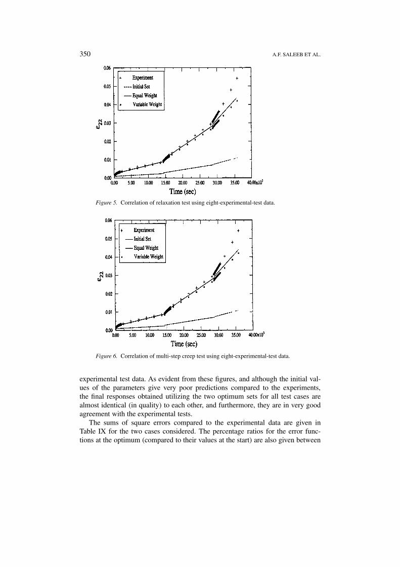
Figure 5. Correlation of relaxation test using eight-experimental-test data.

Figure 6. Correlation of multi-step creep test using eight-experimental-test data.

experimental test data. As evident from these figures, and although the initial val-ues of the parameters give very poor predictions compared to the experiments,the final responses obtained utilizing the two optimum sets for all test cases arealmost identical (in quality) to each other, and furthermore, they are in very goodagreement with the experimental tests.

The sums of square errors compared to the experimental data are given inTable IX for the two cases considered. The percentage ratios for the error func-tions at the optimum (compared to their values at the start) are also given between


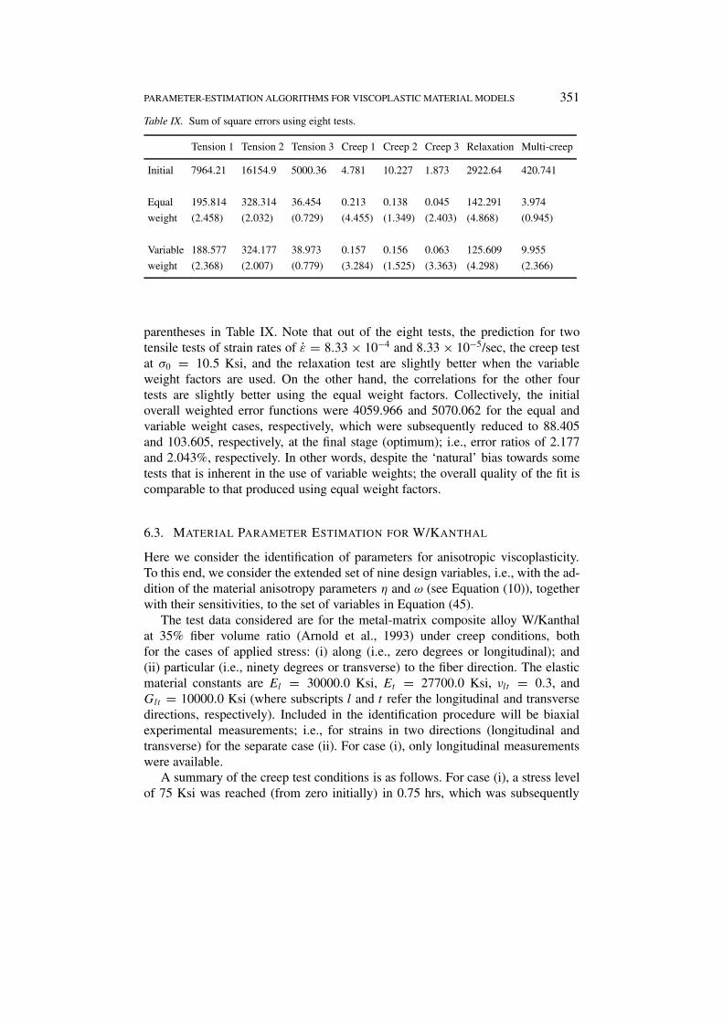
Table IX. Sum of square errors using eight tests.

Tension 1 Tension 2 Tension 3 Creep 1 Creep 2 Creep 3 Relaxation Multi-creep

Initial 7964.21 16154.9 5000.36 4.781 10.227 1.873 2922.64 420.741

Equal 195.814 328.314 36.454 0.213 0.138 0.045 142.291 3.974

weight (2.458) (2.032) (0.729) (4.455) (1.349) (2.403) (4.868) (0.945)

Variable 188.577 324.177 38.973 0.157 0.156 0.063 125.609 9.955

weight (2.368) (2.007) (0.779) (3.284) (1.525) (3.363) (4.298) (2.366)

parentheses in Table IX. Note that out of the eight tests, the prediction for twotensile tests of strain rates of ε̇ = 8.33 × 10−4 and 8.33 × 10−5/sec, the creep testat σ0 = 10.5 Ksi, and the relaxation test are slightly better when the variableweight factors are used. On the other hand, the correlations for the other fourtests are slightly better using the equal weight factors. Collectively, the initialoverall weighted error functions were 4059.966 and 5070.062 for the equal andvariable weight cases, respectively, which were subsequently reduced to 88.405and 103.605, respectively, at the final stage (optimum); i.e., error ratios of 2.177and 2.043%, respectively. In other words, despite the ‘natural’ bias towards sometests that is inherent in the use of variable weights; the overall quality of the fit iscomparable to that produced using equal weight factors.

6.3. MATERIAL PARAMETER ESTIMATION FOR W/KANTHAL

Here we consider the identification of parameters for anisotropic viscoplasticity.To this end, we consider the extended set of nine design variables, i.e., with the ad-dition of the material anisotropy parameters η and ω (see Equation (10)), togetherwith their sensitivities, to the set of variables in Equation (45).

The test data considered are for the metal-matrix composite alloy W/Kanthalat 35% fiber volume ratio (Arnold et al., 1993) under creep conditions, bothfor the cases of applied stress: (i) along (i.e., zero degrees or longitudinal); and(ii) particular (i.e., ninety degrees or transverse) to the fiber direction. The elasticmaterial constants are El = 30000.0 Ksi, Et = 27700.0 Ksi, νlt = 0.3, andGlt = 10000.0 Ksi (where subscripts l and t refer the longitudinal and transversedirections, respectively). Included in the identification procedure will be biaxialexperimental measurements; i.e., for strains in two directions (longitudinal andtransverse) for the separate case (ii). For case (i), only longitudinal measurementswere available.

A summary of the creep test conditions is as follows. For case (i), a stress levelof 75 Ksi was reached (from zero initially) in 0.75 hrs, which was subsequently


Table X. Estimated anisotropic material parameters for W/Kanthal based on twocreep tests.

Material Lower bound Initial Upper bound Optimumparameter

kT 0.20 0.80 8.0 1.705695

n 0.50 1.750 5.0 3.614909

µ 1.0 × 107 5.92 × 1011 1.0 × 1016 6.8738 × 1011

m 1.0 × 10−3 0.345 5.0 0.115448

β 2.0 × 10−4 1.0 × 10−3 5.0 0.93769 × 10−4

R 1.0 × 10−11 0.7126 × 10−6 0.01 4.8494 × 10−7

H 10.0 4.182 × 103 5000.0 2.31008 × 103

ξ 1.0 × 10−1 0.20 0.999 0.201

ζ 1.0 × 10−4 0.216 0.999 0.781218

held constant for a total duration from t = 0.75 to t = 5.15 hrs. For the transverseloading case (ii), the corresponding creep stress level was 25 Ksi (reached in a timeramp of 75 × 10−5 hrs) and was maintained steady afterwards for time between75 × 10−5 to 0.16744 hrs.

Following our previous formats of presenting the results of identifications, weinclude in Table X a summary of the results, i.e., initial, bounding and final valuesof the nine, active, material parameters (including anisotropy).

Note the significant magnitude of the final identified parameters (this is therelevant anisotropic parameter for loading along angles of zero and 90 degreesas in the present case, whereas ξ is only significant for other angles). Without‘some’ biaxial test measurements (e.g., strains in two perpendicular directions), itis almost impossible to determine ‘unique’ values for the anisotropic viscoplasticparameters.

The very good quality of correlations in the two cases (i) and (ii) are shownin Figure 7. Notice also the significant differences in strain magnitudes in the twoperpendicular directions in case (ii).

6.4. MATERIAL PARAMETER ESTIMATION FOR AS4/PEEK PMC AT 25◦C

The material system used in this example is composed of AS4 graphite fibers in apolyether ether Ketone (PEEK) matrix material (Gates and Sun, 1991). A seriesof test specimens having a range of off-axis angles, i.e. fiber-orientation angle(relative to load direction) θ = 15◦, 30◦ and 60◦ were used as presented in Gatesand Sun (1991). In addition, data was presented for each of the fiber angles atdifferent strain rates (Gates and Sun, 1991). For our characterization purposes, an


Figure 7. Anisotropic correlation using two-creep-test data.


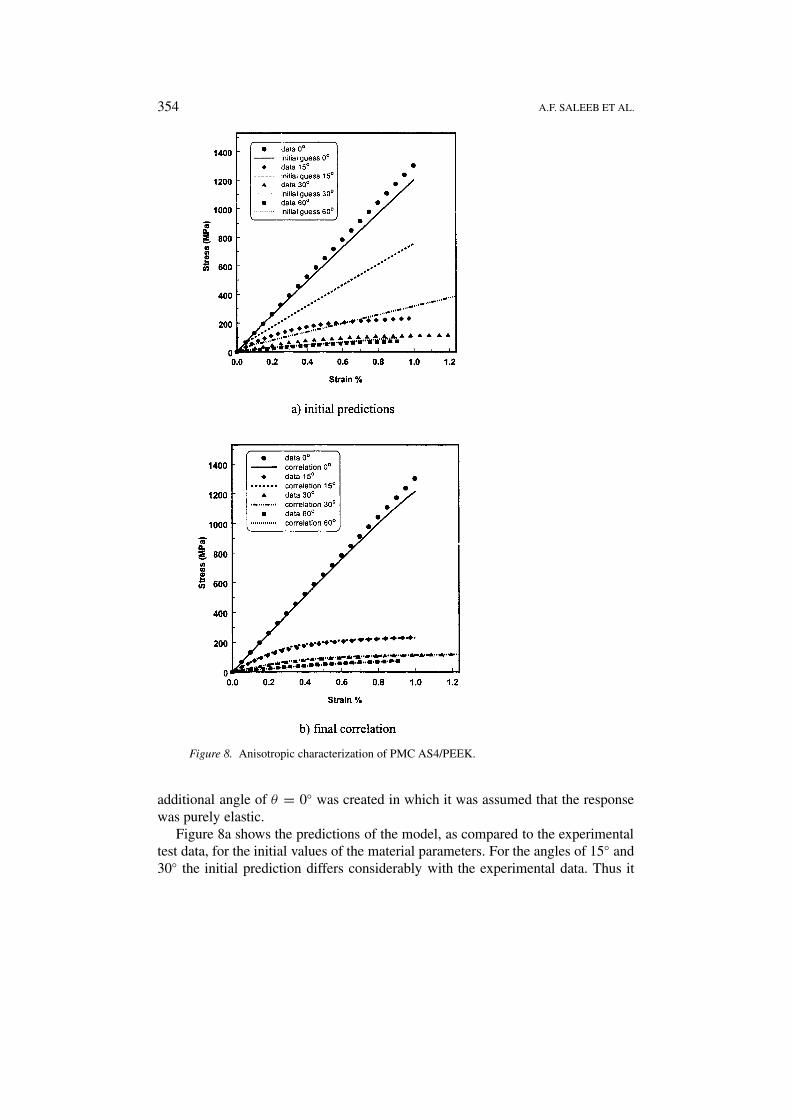
Figure 8. Anisotropic characterization of PMC AS4/PEEK.

additional angle of θ = 0◦ was created in which it was assumed that the responsewas purely elastic.

Figure 8a shows the predictions of the model, as compared to the experimentaltest data, for the initial values of the material parameters. For the angles of 15◦ and30◦ the initial prediction differs considerably with the experimental data. Thus it


Table XI. Final characterized viscoplastic parametersfor PMC at 25◦C.

Material parameters Units Optimum values

κf MPa 0.01

N – 1.80

µ MPa-s 865.15

m(1) – 2

R(1) 1/s 1 × 10−1

κ(1) MPa 41.20

β(1) – 3.55

H(1) MPa 9706.90

ξ – 0.499

ζ – 0.998

can be said that the initial starting values are sufficiently far away from the startingvalues such that the robustness of COMPARE’s ability to fit the data is tested.

The elastic material constants are given as follows: E11 = 130.3 × 103 MPa,E22 = 10.3 × 103 MPa, ν12 = 0.32 and G12 = 0.49 × 105; as required for thein-plane conditions used and these elastic constants were held fixed (passive) asthey were already determined experimentally as in Gates and Sun (1991).

Figure 8b shows the results of COMPARE in which, for all angles, very goodcorrelation with the experimental data is obtained. It is with the exception of the‘artificially very stiff’ response assumed for θ = 0◦, we note that the experimentaldata, together with the model correlation results, for angles θ = 30◦ and 60◦,appear to be heading toward a state of (hardening) saturation.

Finally, note that typically under constant-rate tensile tests, that inelasticprocesses develop relatively fast with short time, thus rendering the physical‘thermal/static recovery’ processes irrelevant during the present tension tests. Cor-respondingly, the parameters R and m (responsible for thermal recovery) werebasically left untouched during the characterization in Table XI.

6.5. MATERIAL PARAMETER ESTIMATION FOR IN738LC AT 850◦C

In this final example we consider the identification of parameters in which bothuniaxial and multi-axial tests are used. This is an extended application of thepresent model, along the lines in Saleeb et al. (2001), with multiple viscoplasticmechanisms (namely three in this case) as alluded to previously at the end of Sec-tion 3.2. The material parameters are to be determined for the IN738LC materialsystem (Abdel-Karim and Ohno, 2000). Included in our characterization were fiveconstant strain rate tensile tests at five different rates, i.e. ε̇ = 1/sec, 10−1/sec,


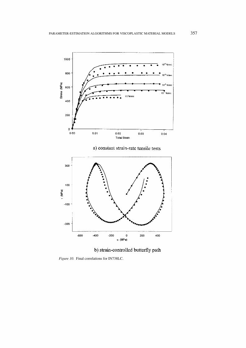
Figure 9. Butterfly strain-control load path. (a) Constant strain-rate tensile tests.(b) Strain-control butterfly path.

10−2/sec, 10−3/sec and 10−4/sec and a multi-axial test, referred to as butterfly-type strain path (Figure 9), a biaxial stress relaxation test which has a tensilepre-strain of ε = 0.424% followed by cyclic shear straining of γ /

√3 = 0.424%

and a biaxial test consisting of a tensile pre-stress of 175 MPa followed by a cyclicshear straining of γ /

√3 = 0.424%. The inclusion of the biaxial tests shows the

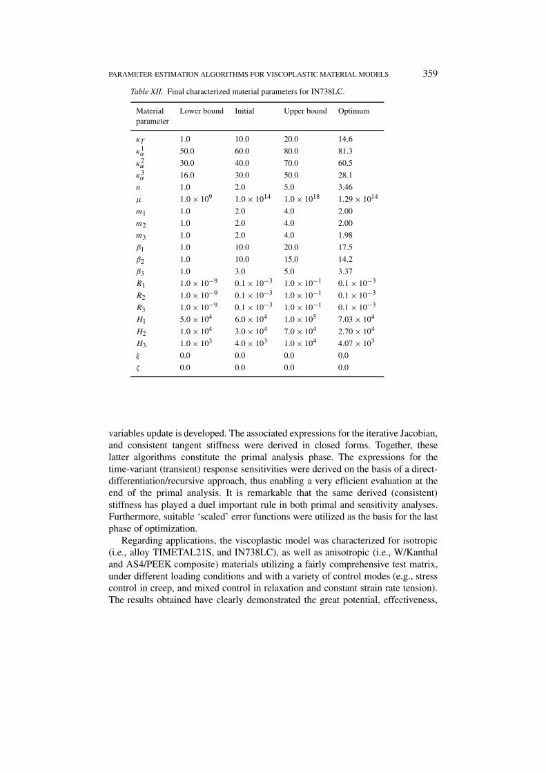
flexibility of COMPARE to handle a variety of load conditions. Thus a total ofseven strain-controlled tests were used in the characterization. The elastic constantsare given as E = 0.15 × 106 MPa and ν = 0.33. Note that in the characterization,three viscoplastic mechanisms were utilized. The results of the characterizationare as shown in Figure 10. Note the excellent correlations with all of the tensiletests, the multi-axial butterfly load test and the stress relaxation test. Table XII liststhe material parameters obtained. Further details of this particular characterizationmay be found in Saleeb et al. (2002).

7. Conclusions

Details of several algorithmic developments have been presented as parts of anoverall automated strategy to estimate the material parameters of a class of visco-plastic models for isotropic and anisotropic responses. These were subsequentlyincorporated into constitutive material estimation software (COMPARE). In this,a general time-stepping algorithm, of the implicit type, for stress- and state-


Figure 10. Final correlations for IN738LC.


Figure 10. Continued.


Table XII. Final characterized material parameters for IN738LC.

Material Lower bound Initial Upper bound Optimumparameter

κT 1.0 10.0 20.0 14.6

κ1α 50.0 60.0 80.0 81.3

κ2α 30.0 40.0 70.0 60.5

κ3α 16.0 30.0 50.0 28.1

n 1.0 2.0 5.0 3.46

µ 1.0 × 109 1.0 × 1014 1.0 × 1018 1.29 × 1014

m1 1.0 2.0 4.0 2.00

m2 1.0 2.0 4.0 2.00

m3 1.0 2.0 4.0 1.98

β1 1.0 10.0 20.0 17.5

β2 1.0 10.0 15.0 14.2

β3 1.0 3.0 5.0 3.37

R1 1.0 × 10−9 0.1 × 10−3 1.0 × 10−1 0.1 × 10−3

R2 1.0 × 10−9 0.1 × 10−3 1.0 × 10−1 0.1 × 10−3

R3 1.0 × 10−9 0.1 × 10−3 1.0 × 10−1 0.1 × 10−3

H1 5.0 × 104 6.0 × 104 1.0 × 105 7.03 × 104

H2 1.0 × 104 3.0 × 104 7.0 × 104 2.70 × 104

H3 1.0 × 103 4.0 × 103 1.0 × 104 4.07 × 103

ξ 0.0 0.0 0.0 0.0

ζ 0.0 0.0 0.0 0.0

variables update is developed. The associated expressions for the iterative Jacobian,and consistent tangent stiffness were derived in closed forms. Together, theselatter algorithms constitute the primal analysis phase. The expressions for thetime-variant (transient) response sensitivities were derived on the basis of a direct-differentiation/recursive approach, thus enabling a very efficient evaluation at theend of the primal analysis. It is remarkable that the same derived (consistent)stiffness has played a duel important rule in both primal and sensitivity analyses.Furthermore, suitable ‘scaled’ error functions were utilized as the basis for the lastphase of optimization.

Regarding applications, the viscoplastic model was characterized for isotropic(i.e., alloy TIMETAL21S, and IN738LC), as well as anisotropic (i.e., W/Kanthaland AS4/PEEK composite) materials utilizing a fairly comprehensive test matrix,under different loading conditions and with a variety of control modes (e.g., stresscontrol in creep, and mixed control in relaxation and constant strain rate tension).The results obtained have clearly demonstrated the great potential, effectiveness,


as well as practical utility of the proposed methodology.1 In particular, a numberof pertinent remarks are summarized below:

(i) Identification exercises were completed successfully from several simulatedas well as available experimental test data.

(ii) The efficiency and accuracy of the developed explicit sensitivities weredemonstrated.

(iii) The size of test sampling points does not appear to have significant effecton the identification, as long as these sample points representative of thetrends/regions of change in the experimental test. However, the data con-tent of tests (e.g., their varieties, duration, etc.) is crucial in ensuring that allparameters will be excited persistently, thus avoiding nonuniqueness.

(iv) Although assigning variable weight factors for tests will naturally case abias towards some tests, the overall quality of the fit was still found to becomparable to that produced using equal weight factors.

(v) Without ‘some’ biaxial test measurements (e.g., strains in two perpendic-ular directions), it is almost impossible to determine ‘unique’ values forthe anisotropic viscoplastic parameters (e.g., compare the no-change versuslarge-change in the shear versus tension-related anisotropy parameters in theidentification of Section 6.3).

Acknowledgement

Partial financial support for this work was provided by NASA Glenn ResearchCenter, Grants No. NCC3-8085 and NAG3-1747 to the University of Akron. Thissupport is gratefully acknowledged.

Note1 The software program COMPARE is available for download as freeware at:

openchannelfoundation.org. Select the Computational Methods Group link for informationon how to download the software.

References

Abdel-Karim, M. and Ohno, N., ‘Kinematic hardening model suitable for ratchetting with steady-state’, Internat. J. Plasticity 16, 2000, 225–240.

Adelmann, H.M. and Haftka, R., ‘Sensitivity analysis of discrete structural system’, AIAA J. 24,1986, 823–832.

Arnold, S.M. and Saleeb, A.F., ‘On the thermodynamic framework of generalized coupled ther-moelastic viscoplastic ‘damage modeling”, Internat. J. Plasticity 10(3), 1994, 263–278.

Arnold, S.M., Saleeb, A.F. and Wilt, T.E., ‘A modeling investigation of thermal and strain inducedrecovery and nonlinear hardening in potential based viscoplasticity’, J. Engrg. Mater. Tech.,ASME 117, 1995, 157–167.


Arnold, S.M., Wilt, T.E., Saleeb, A.F. and Castelli, M.G., ‘An investigation of macro and micro-mechanical approaches for a model MMC system’, HITEMPREVIEW 1993, Advanced HighTemperature Engine Materials Technology Program, Vol. II: Compressor/Turbine Materials-MMC’s/IMC’s, NASA CP 19117, 1993, 52:1–52:12.

Bruhns, O.T. and Anding, D.K., ‘On the simultaneous estimation of model parameters used inconstitutive laws for inelastic material behavior’, Internat. J. Plasticity 15, 1999, 1311–1340.

Bui, H.D. and Tanaka, M. (eds), Inverse Problems in Engineering Mechanics, A.A. Balkema,Rotterdam, 1994.

Chaboche, J.L., ‘Constitutive equations for cyclic viscoplasticity’, Internat. J. Plasticity 5, 1989,247–302.

Chaboche, J.L., ‘Thermodynamic formulation of constitutive equations and application to vis-coelasticity and viscoplasticity of metals and polymers’, Internat. J. Solids Structures 34(18),1997, 2239–2254.

Coleman, B.D. and Gurtin, M.E., ‘Thermodynamics with internal variables’, J. Chem. Phys. 47(2),1967, 597–613.

Freed, A.D. and Walker, K.P., ‘Viscoplasticity with creep and plasticity bounds’, Internat. J.Plasticity 9, 1993, 213–242.

Gates, A.S. and Sun, C.T., ‘Elastic/viscoplastic constitutive model for fiber reinforced thermoplasticcomposites’, AIAA J. 29(3), 1991, 457–463.

Gendy, A.S. and Saleeb, A.F., ‘Nonlinear material parameter estimation for characterizing hyperelastic large strain models’, Comput. Mech. 25(1), 2000, 66–77.

Huang, S. and Khan, A.S., ‘Modeling the mechanical behavior of 1100-0 aluminum at different strainrates by the Bodner–Partom model’, Internat. J. Plasticity 8, 1992, 501–517.

Kojic, M. and Bathe, K.J., ‘Effective-stress function algorithm for thermo-elastic plasticity andcreep’, Internat. J. Numer. Methods Engrg. 24, 1987, 1509–1532.

Lemaitre, J. and Chaboche, J.L., Mechanics of Solid Materials, Cambridge University Press, NewYork, 1990.

Leunberger, D.G., Linear and Nonlinear Programming, 2nd edn., Addison-Wesley, Reading, MA,1984.

Lubliner, J., ‘On the structure of rate equations of materials with internal variables’, Act Mechanica17, 1973, 109–119.

Powell, M.J.D., ‘A fast algorithm for nonlinearly constrained optimization calculations’, in Nu-merical Analysis, G.A. Waston (ed.), Lecture Notes in Mathematics, Vol. 630, Springer-Verlag,Berlin, 1977, 144–157.

Robinson, D.N. and Duffy, S.F., ‘Continuum deformation theory for high-temperature metalliccomposites’, J. Engrg. Mech., ASME 116(4), 1990, 832–844.

Robinson, D.N., Duffy, S.F. and Ellis, J.R., ‘A viscoplastic constitutive theory metal matrix com-posites at high-temperature’, in Thermal Stress, Material Deformation, and ThermomechanicalFatigue, H. Sehitoglu and S.Y. Zamrik (eds), ASME-PVP, Vol. 123, ASME, New York, 1987,49–56.

Saleeb, A.F. and Arnold, S.M., ‘A general reversible hereditary Model: Part I: Theoretical develop-ments’, NASA TM-107493, 1997.

Saleeb A.F. and Wilt, T.E., ‘Analysis of the anisotropic viscoplastic-damage response of compositelaminates-continuum basis and computation algorithms’, Internat. J. Numer. Meth. Engrg. 36,1993, 1629–1660.

Saleeb, A.F., Arnold, S.M. and Castelli, M.G., ‘A general reversible hereditary model: Part II:Application to a titanium alloy’, NASA TM-107494, 1997.

Saleeb, A.F., Wilt, T.E. and Li, W., ‘An implicit integration scheme for generalized viscoplasticitywith dynamic recovery’, Comput. Mech. 21(6), 1998, 429–440.

Saleeb, A.F. Wilt, T.E. and Li, W., ‘Robust integration schemes for generalized viscoplasticity withinternal-state variables’, Internat. J. Comput. & Structures 74, 2000, 601–628.


Saleeb, A.F., Arnold, S.M., Castelli, M.G., Wilt, T.E. and Graf, W., ‘A general hereditarymultimechanism-based deformation model with application to the viscoelastoplastic responseof titanium alloys’, Internat. J. Plasticity 17, 2001, 1305–1350.

Saleeb, A.F., Gendy, A.S., Wilt, T.E. and Trowbridge, D.A., ‘COMPARE-constitutive material para-meter estimation, User’s guide – Version 1.0, Technical Report, Department of Civil Engineering,University of Akron, Akron, OH, 2002.

Schittkowski, K., Nonlinear Programming Code, Lecture Notes in Eronotics and MathematicalSystems, Vol. 183, Springer-Verlag, Berlin, 1980.

Schittkowski, K., ‘NLPQL: A Fortran subroutine solving constrained nonlinear programmingproblems’, in Annals of Operations Research, Vol. 5 C.L. Monma, (ed.), Kluwer AcademicPublishers, Dordrecht, 1986, 485–500.

Schittkowski, K., Solving Nonlinear Least-Squares Problems by a General Purpose SQP-Method,Trends in Mathematical Optimization, International Series of Numerical Mathematics, Vol. 84,Birkhäuser, Boston, MA, 1998.

Senseny, P.E., Brodsky, N.S. and DeVries, K.L., ‘Parameter evaluation for a unified constitutivemodel’, J. Engrg. Mater. Tech., ASME 115, 1993, 157–162.

Vidal, C. and Haber, R.B., ‘Design sensitivity of rate-independent elasto-plasticity’, Comput.Methods Appl. Mech. Engrg. 107, 1993, 393–431.

Welch, B.B., Practical Programming in Tcl and Tk, Prentice Hall, Englewood Cliffs, NJ, 1997.

Parameter-Estimation Algorithms for Characterizing a...

Documents

Transcript of Parameter-Estimation Algorithms for Characterizing a...