Using Modelica/Matlab for parameter estimation in a ... · Using Modelica/Matlab for parameter...

Using Modelica/Matlab for parameter estimation in abioethanol fermentation model

Juan I. Videla Bernt LieTelemark University College

Department of Electrical Engineering, Information Technology, and CyberneticsPorsgrunn, 3901 Norway

Abstract

Bioethanol production from fermentation of a sub-strate using biomass as catalyst is considered.Four alternative reaction rate models with di¤er-ent levels of details are derived and implementedin Modelica. The problem of parameter estima-tion of models using state/parameter estimationtechniques in a Modelica-Dymola/Matlab setup isdiscussed. Practical aspects concerning the di¤er-ent implementations of nonlinear estimators areanalyzed (EKF, UKF, and EnKF). The use ofModelica-Dymola for �on-line� applications suchas state estimation poses the additional problemof the e¢ ciency of the code; this will also be dis-cussed. The four reaction rate models are �ttedusing �ctitious experimental data generated fromone of the models to illustrate the parameter esti-mation procedure.Keywords: bioethanol fermentation, parameter es-timation, nonlinear estimators

1 Introduction

Alcoholic fermentation is an important bio-chemical process which has been known for some5000 years. Ethyl alcohol, or more commonlyethanol, has chemical formulae C2H5OH, and�nds uses as (i) alcoholic beverage (beer, wine,spirits), (ii) solvent, (iii) raw material in chemicalsynthesis, and (iv) fuel.With the current focus on CO2 release and globalwarming, there is a considerable interest in pro-ducing fuel from biomass. Production of ethanolfrom fermentation typically involves a two stepprocess: (a) the main process where substrate(glucose) is converted to ethanol and non-fossilCO2 in an enzymatic process, and (b) the aero-

bic yeast growth through the consumption of sub-strate and oxygen.

In continuous reactors, yeast is contiuouslywashed out, leading to a less e¢ cient use of theyeast. The use of immobilized yeast increasesthe e¢ ciency of the process, as less substrate is�wasted� for yeast production. In fermentation,salts are involved as co-enzymes. The resultingions a¤ect the oxygen uptake in the reaction mix-ture.

The produced (bio-) ethanol can be used as fuelafter some additional processing ��lter yeast, re-move water by distillation, etc. Alternatively, theethanol can be converted to methane by microor-ganism.

The e¢ cient production of ethanol in a fermenta-tion reactor requires quantitative analysis of howraw materials are converted to products. Staticmodels are often used for design purposes for con-tinuous reactors, while dynamic models are re-quired for batch reactors (e.g. beer production)and for control analysis and design in continuousreactors. A simple numeric dynamic model forthe continuous fermentation of glucose using theyeast saccharomyces cerevisae is given in [1]. Themodel is somewhat simpli�ed in that the dynam-ics of the overall reactor volume is neglected, therole of the salts as co-enzymes is neglected, andsomewhat simple kinetic reaction rates are used.A more systematic development of reaction ratesfor the continuous ethanol fermentation process ispresented in [2]. In [1], the e¤ect of ions on theoxygen uptake in the reactor mixture is included,but the e¤ect of glucose is neglected; expressionsfor the e¤ect of ions and sugars are given in [3].Most of the parameters of the model of [1] aregiven in their publication; however there is oneor two typos, and the e¤ect of salt ions on the

Using Modelica/Matlab for Parameter Estimation in a Bioethanol Fermentation Model

The Modelica Association 287 Modelica 2008, March 3rd − 4th, 2008

oxygen uptake is as if the salinity of the reactionmixture was similar to that of sea water (due tosome mole-to-gram conversion problem).

It is of interest to study the parameter estima-tion problem of the fermentation model for thedi¤erent rates of reaction models with the pur-poses of control and identi�cation. Online pa-rameter identi�cation can be achieved using re-cursive state/parameter estimators. For linearsystems with normally distributed process andmeasurement noise, the optimal recursive estima-tor is the Kalman �lter. Estimation for non-linear systems is considerably more di¢ cult andadmits a wider variety of suboptimal solutions.The extended Kalman �lter (EKF), unscentedKalman �lter (UKF), and the ensemble Kalman�lter (EnKF) are implemented using Modelica-Dymosim and Matlab. The fermentation with thedi¤erent reaction rates is implemented in Model-ica and compiled into Dymosim. The parametersare directly estimated using the parameter state-augmented approach and the discrete version ofthe estimators are implemented in Matlab.

The paper is organized as follows. In the nextsection, an overview of the fermentation processand its implementation is given. Di¤erent kineticreaction rates for the fermentation process are pre-sented in accordance with biochemical engineeringprinciples. We give a brief introduction of the im-plementation of the proposed models in Modelica.In section 3, we discuss the problem of parame-ter estimation of models using recursive nonlinearstate/parameter estimation techniques in a Mod-elica/Matlab setup. The traditional use of theExtended Kalman Filter poses some questions re-garding the computation of the Jacobians of thesystem. In more modern techniques such as theUnscented Kalman Filter, and Monte Carlo tech-niques such as the Ensemble Kalman Filter, thecomputation of Jacobians is avoided. Also, thesemore modern techniques handle nonlinearities in abetter way than the Extended Kalman Filter. Inparticular when these estimation techniques areused for parameter estimation, some of the �l-ter constants need to be carefully tuned, and wediscuss this problem. Also, the use of Modelicafor �on-line�application such as state estimationposes some particular problems with regards tothe e¢ ciency of Modelica implementations; thiswill be discussed. Finally, we assume that themodel of [1] has been �tted well to experimen-

tal data. We then generate �ctitious experimentaldata from the model of Agachi et al., and we illus-trate the parameter estimation procedure by �t-ting the new models to the generated experimentaldata.

2 Fermentation model

2.1 Description

The nutrients in biochemical reactions are knownas substrates. The substrate for the ethanol pro-duction process is thus glucose. For the yeastgrowth process, the substrates are glucose andoxygen. In the sequel we will use symbol S do de-note glucose. Since oxygen has a relatively simplechemical formulae, we will not introduce a partic-ular notation for oxygen. Furthermore, we will usesymbol P for the main product, which is ethanol,and symbol X for the yeast.The original reaction kinetics given by [1] can beseen in Table 3 with the superscript o for everyspecie roj :The fermentation reactor for the production ofethanol is sketched in Fig. 1. Glucose (substrateS, sugar) in a water solution is continuously fedto the well stirred reactor; the volumetric feed�ow is _Vi [volume/time] : The reactor containsyeast (microorganisms X), which reacts with sub-strate to produce ethanol (product P). We con-sider this reaction 1, with kinetic reaction rater1 [mass/(volume time)] 1.

SE1! P (1)

Simultaneously, in a second reaction (2), the mi-croorganism breed under the consumption of oxy-gen to produce more yeast; the kinetic reactionrate is r2 [mass/(volume time)].

S+O2E2! X (2)

The relationships between the rates of generationrj [mass/(volume time)] with j 2 fP;X;S;O2gcan be seen in Table 3. All reaction rates havedimension mass/(volume time). It follows thatr1 = rP is the mass of ethanol produced per vol-ume and time, etc. Factor YSP has the meaningof mass of ethanol (product) produced per mass ofglucose (substrate) consumed. Similar interpreta-tions are valid for YSX and YOX.

1The CO2 specie is not considered in the expression.

J. I. Videla, B. Lie


V% i,_,_S,i,Ti

V% o,_,_P,_X,_S,_CO2 ,T

V, h,_,_P,_X,_S,_CO2 ,T

A

Q%V% J,_J, TJ,i V% J,_J,TJ

Fig. 1: Sketch of fermentation reactor.

Both in the inlet stream and in the reactionmedium, water is dominant such that the density� of the mixture can be assumed to be constant.For oxygen, there is an input �ow _mO2;a in thatoxygen is transported from air to dissolved oxygenin the reaction medium,

_mO2;a = kà��O2 � �O2

�V; (3)

where kà [1/time] depends on the temperature,V is the volume of the reaction medium, �O2 isthe mass based concentration [mass/volume], and��O2 is the equilibrium concentration of oxygen inwater. ��O2 depends on salts in the mixture. Itis assumed that there is no O2 in the feed waterstream. In both reactions 1 and 2, CO2 is releasedas a byproduct; here we do not model the carbondioxide production.The total mass, species balances, and energy bal-ance for the reactor and the water jacket modelsare presented in Table 1. The fermentation bound-ary conditions de�ned as inputs and outputs arede�ned in this table. The fermentation model pa-rameters of the original model developed in [1] areshown in Table 2.

2.1.1 Fermentation reaction and rates

The elementary reaction rate re1 for the ethanolproduction is developed considering the substrate-enzyme interactions, the resulting rate is given bythe Michaelis-Menten kinetics. Additionally, thepresence of ethanol inhibits the ethanol produc-

Tab. 1: Fermentation model.Reactor total mass and species balances:ddtm = _mi � _mo

ddtmj = _mj;i � _mj;o + _mk

j;g with j 2 fP;X;S;O2gReactor rates of generation:

_mj;g = rkj V with j 2 fP;X;S;O2g

Reactor outputs:

_mo = kpV

_mj;o = _Vo�j with j 2 fP;X;S;O2gReactor inputs:

_mi = � _Vi

_mP;i � 0_mX;i � 0_mS;i = �S;i

_Vi

_mO2= _mO2;a

Oxygen interface transport:

_mO2;a = kà��O2

� �O2

�V

��O2= ��O2;0

(T ) exp (�P

n In �P

m Sm)

with n 2 fNa+;Cl�;Ca+2;CO�23 ;Mg+2;H+;OH�g

In =12Hjz

2j cjP

m Sm = SS = KScS��O2;0

(T ) = �0 + �1T + �2T2 + �3T

3

Reactor energy balance:

�cpVdTd = �cp _Vi (Ti � T ) + �Hr;2V rjO2

� _Qheatex

Water jacket mass balance:

_mJ;i + _mJ;o = 0

Water jacket energy balance:

�J cp;JVJdTJdt = �J cp;J

_VJ (TJ;i � TJ) + _Qheatex

Water jacket-reactor heat transfer:

Qheatex = UxAx (T � TJ)

tion rate (inactive enzymes), this e¤ect is also in-cluded in this reaction rate. The combined e¤ectis shown in Table 3.A common simpli�ed model for the e¤ect of com-petition for active sites yields the simpli�ed raters1; where a specie that competes for an activesite and participate in the reaction has the form�S=(KS;1+�S), while a specie that competes for anactive site and does not participate in the reactionhas the form 1=(1 + kP;1�P):

Another possible model for ethanol produc-tion with ethanol inhibition is to notice thatexp

��kP;1�P

�� 1=

�1 + kP;1�P

�: This exponen-

tial term can be explained by assuming inhibitionby ethanol may be caused by intracellular mech-anisms.A similar analysis can be done for the reactionrate for the yeast production for the di¤erent ap-



Tab. 2: Parameters for the fermentation reactor withoriginal reaction rates.Reactor/Water jacket parameters:

� = 1080 g= l � ~Hr;O2= �518 kJ=molO2

�J= 1000 g= l VJ= 50 l

cp= 4:18 J=( g�C) UxAx= 3:6E5 J= ( h

�C)

cp;J= 4:18 J=( g�C) (kla)0= 38h

�1

Rate of generation parameters:

�1= 1:79 h�1 KS;2= 1:03 g= l

�O2= 0:5 h�1 KO2

= 8:86mg= l

A1= 9:5E8 h�1 kP;1= 0:070 l= g

A2= 2:55E33 h�1 kP;2= 0:139 l= g

Ea1=R = 6:6185E3 K YSX= 0:607 gX= gSEa2=R = 26:474E3 K YSP= 0:435 gP= gSKS;1= 1:68 g= l YOX= 0:970 gX= gO2

Oxygen interface transport parameters:

zNa+= +1 HMg+2= �0:314 l=molzCl�= �1 HCa+2= �0:303 l=molzCa+2= +2 KS= 0:119 l=mol

zCO�23= �2 MNaCl= 58:44 g

zMg+2= +2 MMgCl2= 95:21 g=mol

zH+= +1 MCaCO3= 100:09 g=mol

zOH�= �1 MO2= 32 g=mol

HNa+= �0:55 l=mol MS= 180:15 g=mol

HCl�= 0:84 l=mol �0= 14:16mg= l

HOH�= 0:94 l=mol �1= �0:394mg=( l �C)HCO�2

3= 0:48 l=mol �2= 7:71E�3mg=( l �C2)

HH+= �0:77 l=mol �3= �6:4E�5mg=( l �C3)

proximations.The original rates are closely related to the devel-oped rates where product inhibition is explainedvia intracellular transport. The original modelneglects the oxygen dependence of the intracellu-lar model and neglects the substrate dependenceand the product inhibition. Clearly, when the ki-netic rates change their functional form, the para-meter/temperature functions change. The di¤er-ent rate reaction rates are shown in Table 3.

2.2 Implementation

In Modelica it is important to implement a goodstructure to enable easy modi�cation of the mod-els. The core model of the fermentation reactor isthe basic volume model, there is where the totalmass, species mass balances, and energy balanceare de�ned. This model exchanges heat with thewater jacket model through an MSL heat port. It

Tab. 3: Parameters for the fermentation reactor withoriginal reaction rates.Reaction rates 1:

ro1= �1�X�S

KS;1+�Sexp

��kP;1�P

�re1= �1�X

�SKS;1+(1+kP;1�P)+�S

rs1= �1�X�S

KS;1+�S

11+kP;1�P

ri1= �1�X�S

KS;1+�Sexp

��kP;1�P

�Reaction rates 2:

ro2= �2�X�S

KS;2+�Sexp

��kP;2�P

�re2= �2�X

�S�O2KS;2KO2

+(1+kP;2�P)+KO2�S+�S�O2

rs2= �2�X�S

KS;2+�S

�O2KO2

+�O2

11+kP;2�P

ri2= �2�X�S

KS;2+�S

�O2KO2

+�O2exp

��kP;2�P

�Rates of reactions for P;X;S;O2rkP= r

k1 , k = fo; e; s; ig

rkX= rk2 , k = fo; e; s; ig

rkS= � 1YSPrk1� 1

YSXrk2 , k = fo; e; s; ig

rk�

O2= � 1

YOXrk

�

2 , k�= fe; s; igroO2

= � 1YOX

�O2�X

�O2KO2

+�O2

also has a chemical port (i.e. intensive variables:temperature and mass concentration vector; andextensive variables: mass �ow rates vector andheat �ow rate) that connects with the rate of gen-eration replaceable model and the oxygen trans-port model, and two thermo�uid ports (i.e. in-tensive variables: pressure, speci�c enthalpy, andmass fraction vector; and extensive variables: en-thalpy �ow rate vector, mass �ow rate vector, andtotal mass �ow rate) to connect the basic volumewith the incoming mass �ow rate in and the out-coming mass �ow rate out of the model. The ba-sic volume is then connected to the water jacketmodel, to the oxygen transport model, to the rateof generation replaceable model as shown in Fig.2.

The four di¤erent reaction kinetic rates (i.e. orig-inal, elementary, simpli�ed, and intracellular) areimplemented using a replaceable component. Acommon set of parameters and equations are de-�ned in a partial model called rate of generation.Speci�cs of every reaction rate model are de�nedseparately in each model that inherits the rate ofgeneration partial model. The heat of reaction isalso de�ned in these models. The water jacketmodel uses two MSL �ow ports.



O2 transportinterface model

Water Jacketmodel

Mass andenergy balancecontrol volume

replaceablerate of

generationmodels

Fig. 2: Dymola diagram layout of the fermentation re-actor component.

3 Nonlinear estimators

3.1 Description

The ethanol fermentation reactor model can bewritten in the general discrete nonlinear statespace form:

xk = fk�1 (xk�1; uk�1; wk�1)

yk = hk (xk; vk) (4)

where fk�1 : Rnx+nu+nw ! Rnx is the discretestate function, xk 2 Rnx is the discrete state vec-tor, uk�1 2 Rnu is the discrete input, wk�1 2 Rnwis the discrete process noise vector, hk : Rnx+nv !Rnx is the discrete output function, vk 2 Rnv is thediscrete measurement noise vector, yk 2 Rny is theoutput vector, and k is the time index. The noisevector sequences fwk�1g and fvkg are assumedGaussian, white, zero-mean, uncorrelated, andhave the known covariance matrices Qk 2 Rnx�nwand Rk 2 Rny�nv .

3.2 Augmented states

The augmented state space approach can be di-rectly used to simultaneously solve the state andthe parameter estimation problem (e.g. see [4]).An augmented state space representation is for-mulated by adding the vector of parameters to beestimated �k 2 Rn��1 as new states:

Tab. 4: EKF algorithm.

Initialization:x0j0 � N (�x0; P0)P0j0 = P0

for k = 1; 2; : : :

Propagation step:( a priori covariance estimate)

Fk�1 =@fk�1@xk�1

��xk�1jk�1

Lk�1 =@fk�1@wk�1

��xk�1jk�1

Pkjk�1 = Fk�1Pk�1jk�1FTk�1 + Lk�1Qk�1L

Tk�1

( a priori state-output estimate)

xkjk�1 = fk�1(xk�1jk�1; uk�1; 0)

ykjk�1 = hk(xkjk�1; 0)

Measurement update:(Kalman gain calculation)

Hk =@hk@uk

��xkjk�1

Mk =@hk@vk

��xkjk�1

Kk = Pkjk�1HTk (HkPkjk�1H

Tk +MkRkM

Tk )

�1

( a posteriori state-covariance estimate)

xkjk = xkjk�1 +Kk(yk � ykjk�1)Pkjk = (I �KkHk)Pkjk�1

"xk

�k

#=

"fk�1

�xk�1; uk�1; w

(x)k�1

��k�1 + Tsw

(�)k�1

#(5)

yk = hk (xk; vk) (6)

where Ts is the sampling time step, w(x)k�1 2 Rn

(x)w

is the process noise vector that a¤ects the original

states; and w(�)k�1 2 Rn(�)w is the process noise vec-

tor that a¤ects the added parameter states. Thenoise vector sequences fwk�1g and fvkg are as-sumed Gaussian, white, zero-mean, uncorrelated,and have the known covariance matrices Qk 2R(nx+n�)�(n

(x)w +n

(�)w ) and Rk 2 Rny�nv

wk � N (0;blkdg(Q(x)k ; Q(�)k ))

vk � N (0; Rk)

During the propagation step, the augmentedstates corresponding to parameters �k are consid-ered equal to the previous time step �k�1 withsome additive process noise w(�)k�1. If it is assumedthat the parameters do not change at all, thenthere is no process noise vector w(�)k�1, but for themore general case of time-varying parameters (e.g.fouling, etc.), the value of Q(�)k will be given bythe admissible range of variation of �k: During



the measurement update step the parameter val-ues are corrected.For notational simplicity in the estimators algo-

rithms that follow, the augmented state vector isreferred to as xk, the state augmented function (5)is referred to as fk�1, and the augmented processnoise vector is referred to as wk�1.

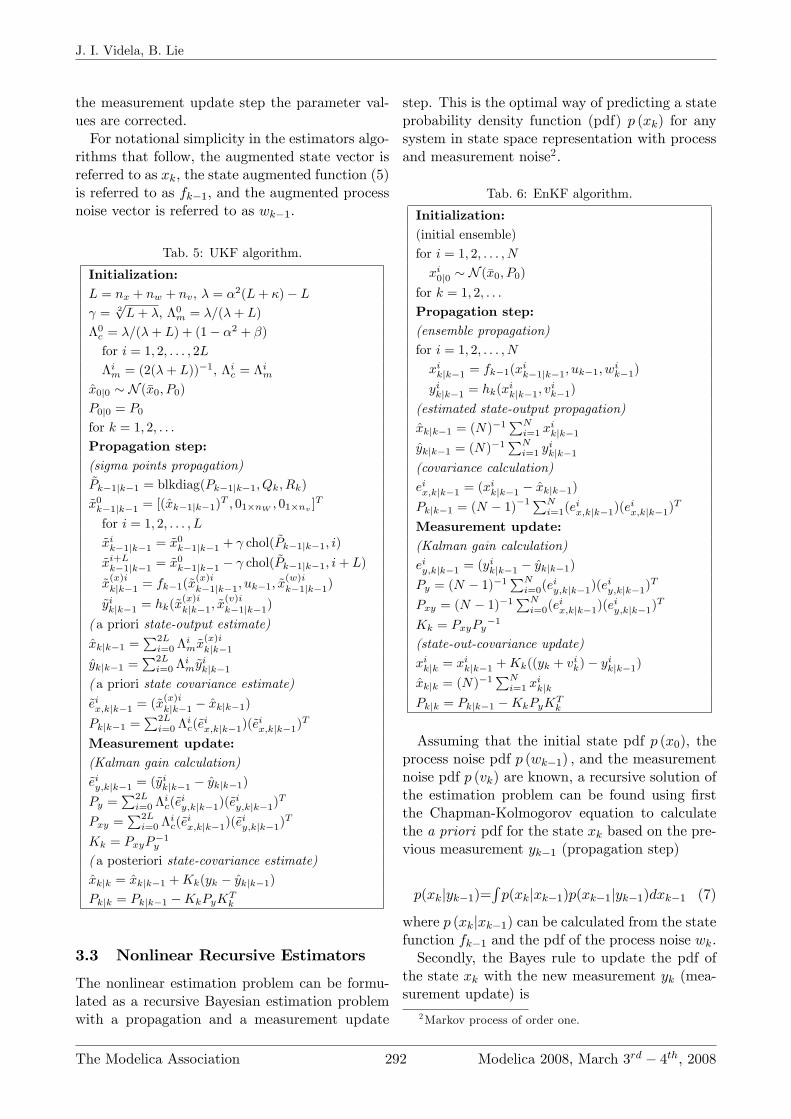
Tab. 5: UKF algorithm.

Initialization:L = nx + nw + nv; � = �

2(L+ �)� L = 2

pL+ �; �0m = �=(�+ L)

�0c = �=(�+ L) + (1� �2 + �)for i = 1; 2; : : : ; 2L

�im = (2(�+ L))�1; �ic = �

im

x0j0 � N (�x0; P0)P0j0 = P0

for k = 1; 2; : : :

Propagation step:(sigma points propagation)~Pk�1jk�1 = blkdiag(Pk�1jk�1; Qk; Rk)

~x0k�1jk�1 = [(xk�1jk�1)T ; 01�nW ; 01�nv ]

T

for i = 1; 2; : : : ; L

~xik�1jk�1 = ~x0k�1jk�1 + chol(

~Pk�1jk�1; i)

~xi+Lk�1jk�1 = ~x0k�1jk�1 � chol( ~Pk�1jk�1; i+ L)

~x(x)ikjk�1 = fk�1(~x

(x)ik�1jk�1; uk�1; ~x

(w)ik�1jk�1)

~yikjk�1 = hk(~x(x)ikjk�1; ~x

(v)ik�1jk�1)

( a priori state-output estimate)

xkjk�1 =P2L

i=0 �im~x

(x)ikjk�1

ykjk�1 =P2L

i=0 �im~y

ikjk�1

( a priori state covariance estimate)

~eix;kjk�1 = (~x(x)ikjk�1 � xkjk�1)

Pkjk�1 =P2L

i=0 �ic(~e

ix;kjk�1)(~e

ix;kjk�1)

T


~eiy;kjk�1 = (~yikjk�1 � ykjk�1)

Py =P2L

i=0 �ic(~e

iy;kjk�1)(~e

iy;kjk�1)

T

Pxy =P2L

i=0 �ic(~e

ix;kjk�1)(~e

iy;kjk�1)

T

Kk = PxyP�1y

( a posteriori state-covariance estimate)

xkjk = xkjk�1 +Kk(yk � ykjk�1)Pkjk = Pkjk�1 �KkPyK

Tk

3.3 Nonlinear Recursive Estimators

The nonlinear estimation problem can be formu-lated as a recursive Bayesian estimation problemwith a propagation and a measurement update

step. This is the optimal way of predicting a stateprobability density function (pdf) p (xk) for anysystem in state space representation with processand measurement noise2.

Tab. 6: EnKF algorithm.

Initialization:(initial ensemble)

for i = 1; 2; : : : ; N

xi0j0 � N (�x0; P0)for k = 1; 2; : : :

Propagation step:(ensemble propagation)

for i = 1; 2; : : : ; N

xikjk�1 = fk�1(xik�1jk�1; uk�1; w

ik�1)

yikjk�1 = hk(xikjk�1; v

ik�1)

(estimated state-output propagation)

xkjk�1 = (N)�1PN

i=1 xikjk�1

ykjk�1 = (N)�1PN

i=1 yikjk�1

(covariance calculation)

eix;kjk�1 = (xikjk�1 � xkjk�1)

Pkjk�1 = (N � 1)�1PN

i=1(eix;kjk�1)(e

ix;kjk�1)

T


eiy;kjk�1 = (yikjk�1 � ykjk�1)

Py = (N � 1)�1PN

i=0(eiy;kjk�1)(e

iy;kjk�1)

T

Pxy = (N � 1)�1PN

i=0(eix;kjk�1)(e

iy;kjk�1)

T

Kk = PxyPy�1

(state-out-covariance update)

xikjk = xikjk�1 +Kk((yk + v

ik)� yikjk�1)

xkjk = (N)�1PN

i=1 xikjk

Pkjk = Pkjk�1 �KkPyKTk

Assuming that the initial state pdf p (x0), theprocess noise pdf p (wk�1) ; and the measurementnoise pdf p (vk) are known, a recursive solution ofthe estimation problem can be found using �rstthe Chapman-Kolmogorov equation to calculatethe a priori pdf for the state xk based on the pre-vious measurement yk�1 (propagation step)

p(xkjyk�1)=Rp(xkjxk�1)p(xk�1jyk�1)dxk�1 (7)

where p (xkjxk�1) can be calculated from the statefunction fk�1 and the pdf of the process noise wk.Secondly, the Bayes rule to update the pdf of

the state xk with the new measurement yk (mea-surement update) is

2Markov process of order one.



p (xkjyk)=p (ykjxk) p (xkjyk�1)Rp (ykjxk) p (xkjyk�1) dxk

(8)

where p (ykjxk) is available from our knowledgeof the output function hk and the pdf of vk, andp (xkjyk�1) is known from (7). Although the initialstate pdf p (x0), the process noise pdf p (wk�1) ;and the measurement noise pdf p (vk) are neededto solve the recursive Bayesian estimation, no spe-ci�c statistical distribution is required.The recursive relations (7) and (8) used to cal-

culate the a posteriori pdf p (xkjyk) are a con-ceptual solution and only for very speci�c casescan these be solved analytically. In general, ap-proximations are required for practical problems.Three main groups of suboptimal techniques withsigni�cant performance and computational costdi¤erences are used to approximate the recursiveBayesian estimation problem: the classical non-linear extension of the Kalman �lter (EKF), theUnscented Kalman �lter (UKF), and the Ensem-ble Kalman �lter (EnKF) approaches.

3.4 Extended Kalman Filter (EKF)

The discrete EKF is probably the most used se-quential nonlinear estimator nowadays. It wasoriginally developed as a nonlinear extension bySchmidt [5] of the seminal work of Kalman [6].Based on the Kalman �lter, it assumes that thestatistical distribution of the state vector remainsGaussian after every time step3 so it is only nec-essary to propagate and update the mean and co-variance of the state random variable xk. Themain concept is that the estimated state (i.e. es-timated mean of xk) is su¢ ciently close to thetrue state (i.e. true mean of xk) so the nonlinearstate/output model equations can be linearizedby a truncated �rst-order Taylor series expansionaround the previously estimated state.The discrete algorithm is given in table 4. In

general, this algorithm works for many practicalproblems, but no general convergence or stabilityconditions can be established4 and its �nal per-formance will depend on the speci�c case study.For highly nonlinear models with unknown initialconditions, the EKF assumptions may prove tobe poor and the �lter may fail or have a poor per-

3 this assumption is in general not true for nonlinear sys-tems.

4except for some special cases [7].

dymosim i generates adefault dsin.txt file

Statistics ofthe simulation. Debug info

Results of thesimulation Binary or textformats

Final state(same structure

as dsin.txt)

Standaloneprogram that

s simulatel linearizet inival. calc.

Optional fileto definetrajectories ofinput signals

Experiment description:start timestop timeinival. (opt.)parameters,etc

dymosim l linearize modelat initial valuesJacobians

dymosim.exe

dslog.txt dsres.matdsres.txt dsfinal.txt

dsin.txtdsu.matdsu.txt

dslin.mat

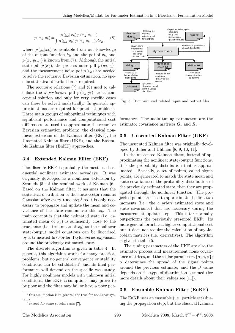
Fig. 3: Dymosim and related input and output �les.

formance. The main tuning parameters are theestimator covariance matrices Qk and Rk:

3.5 Unscented Kalman Filter (UKF)

The unscented Kalman �lter was originally devel-oped by Julier and Uhlman [8, 9, 10, 11].In the unscented Kalman �lters, instead of ap-

proximating the nonlinear state/output functions,it is the probability distribution that is approx-imated. Basically, a set of points, called sigmapoints, are generated to match the state mean andstate covariance of the probability distribution ofthe previously estimated state, then they are prop-agated through the nonlinear function. The pro-jected points are used to approximate the �rst twomoments (i.e. the a priori estimated state andstate covariance) that are necessary during themeasurement update step. This �lter normallyoutperforms the previously presented EKF. Itsmore general form has a higher computational costbut it does not require the calculation of any Ja-cobian matrices (i.e. derivatives). The algorithmis given in table 5.The tuning parameters of the UKF are also the

estimator process and measurement noise covari-ance matrices, and the scalar parameters f�; �; �g:� determines the spread of the sigma pointsaround the previous estimate, and the � valuedepends on the type of distribution assumed (formore details about their values see [11]).

3.6 Ensemble Kalman Filter (EnKF)

The EnKF uses an ensemble (i.e. particle set) dur-ing the propagation step, but the classical Kalman



measurement update equations (instead of usingthe resampling with replacement approach of theparticle �lters) during the measurement updatestep. The covariances matrices Pxy and Py ob-tained from the propagation of the ensemble ele-ments through the nonlinear state-space are usedto calculate the Kalman gain Kk: The a posteri-ori ensemble is calculated from the Kalman gainmatrix and an arti�cially generated measurementparticle set that is normally distributed with meanequal to the current measurement yk and covari-ance equal to Rk. The a posteriori ensemble isused to calculate the a posteriori state and co-variance estimate, and it is used for the next �lteriteration of the algorithm. For details about thealgorithm, see table 6. The EnKF was originallydeveloped in [12] to overcome the curse of dimen-sionality in large scale problems (i.e. weather dataassimilation). It is suggested in the literature [13]that ensembles (i.e. particle sets) of 50 to 100are often adequate for systems with thousands ofstates, but no conclusive work has been done onthis.

Besides the estimator process and measurementnoise covariance matrices, the other tuning para-meter for this �lter is the number of ensemble el-ements.

3.7 Implementation

The fermentation model is written in Modelicaand compiled in Dymola into a stand-alone ex-ecutable �le called Dymosim. The di¤erent es-timators are implemented in Matlab from whereDymosim is sequentially called during the prop-agation step to project the state vector (i.e. in-tegrate over the sampling time) in the estimatoralgorithms. The parameter state vector �k is di-rectly propagated within the Matlab code so theoriginal model does not need to be modi�ed toinclude the parameter dynamic equations.

Within the Modelica model the input vector uk,the process noise input vector wk, and the para-meter input vector �k must be de�ned. This canbe done in the following way at the top level ofthe model:

model fermentation...input Real u_u1; // define model inputsinput Real u_w1; // define noise inputsinput Real u_p1; // define param. inputs...parameter Real p_u1;parameter Real p_w1;parameter Real p_p1;parameter Real p_i1;equationfluidBCv.u[1]=u_u1+p_u1;reactor.basicVol.w[1]=u_w1+p_w1;reactor.RG.p_mu1=u_p1+p_p1;reactor.i_rho[1]=p_i1;

end fermentation;

Additionaly, the discrete EKF estimator re-quires the calculation of the discrete JacobiansFk�1; Lk�1;Hk;Mk. This can be done calculat-ing a linearized model around the previous stateestimate de�ned by the operating point op =[xTk�1; u

Tk�1; 0; �

Tk�1]

T with the following Matlabcode:

eval( ['! dymosim ', 'l ','dsin.txt'] );

In the �le �dsin.txt� (see Fig. 3) the operatingpoint is de�ned using parameters and the initialstate for every iteration. The calculated linearizedmodel is written in the �le �dslin.mat�and then itcan be loaded into Matlab using the Dymola add-on function tloadlin which loads the matricesA,B,C,D and the string vectors uname, yname, andxname. These matrices correspond toA = @f(x;u;w)

@x

��op

B =�@f(x;u;w)

@u

��op; @f(x;u;w)@w ;

��op; @f(x;u;w)@�

��op

�C = @h(x;u)

@x

��op

D = @h(x;u)@u

��op

The parameter augmented state space discrete ja-cobians are approximated from the A;B;C;D ma-trices

Ae =

"A B(:;nu+nw+1:end)

0np�nx 0np�np

#Fk�1 = @fk�1

@xk�1

��op� exp (Ae�t)

Be =

"B(:;nu+1:end) 0nx�np0np�nx 1np�np

#Lk�1 = @fk�1

@wk�1

��op

� [I�t+ 12!A

e�t2 + 13!A

e2�t3 + : : :]Be

Hk =�C 0ny�nx

�Mk = D



where nu is the input vector dimension, nw is theprocess noise vector dimension, and so on. Fornotation simplicity, the matrices in the previousequations use Matlab notation.

4 Results

Due to the lack of experimental measurements,simulated data sets from the model with the orig-inal kinetic reaction rates are generated. The sys-tem model is simulated for 1000 h and data sam-ples are collected every 1 h. Because the transientresponse is relevant to parameter identi�cation,step-like input sequences with high frequency con-tent are used (see Fig.4). The initial state vectorfor the fermentation model isx0 =

h_V ; �P; �X; �S; �O2

; T; TJ

iT 0= [1000; 12:9; 0:9; 28:6; 3:9; 30:4; 26:9]

T

The system model process and measurement noisevector sequences fwk�1g and fvkg are Gaussian,white, zero-mean, uncorrelated, and have constantcovariance matricesQk = blkdiag

�Q(x)k ; Q

(�)k

�Q(x)k = diag ([1000; 15; 2; 100; 5; 35; 30]) � 1E�7

Q(�)k = diag ([1; 1; 1; 1; 1; 1; 1; 1]) � 1E�7

Rk = diag ([15; 2; 100; 5; 35; 30]) � 2E�3A subset of 8 parameters � =[�1;KS;1;KS;2; kP;1; kP;2; YSP; YSX; YOX]

T isestimated for every estimator (i.e., the EKF,the UKF, and the EnKF) using every reactionrate model (i.e., the original, the elementary,the simple, and the intracellular reaction kineticmodels). The initial parameter values for everyreaction rate model are adjusted to ensure thatall simulation results give the same steady statevalues at initial time t = 0. The estimatorsinputs are equal to the system model inputsu = [ _VJ;i; �S;i]

T , and the measured outputs arey = [�P; �X; �S; �O2 ; T; TJ ]

T (see Fig.4). The esti-mators are simulated for 1000 h with a samplingtime of 1 h.The estimators� initial state vectors are drawnfrom a normal distribution with mean and covari-ance equal tox0j0 � N ([�xT0 ; ��

T0 ]T ;blkdiag

�P(x)0 ; P

(�)0

�)

�x0 = [990; 13:9; 0:8; 27:6; 4:9; 27:4; 24:9]T

��0 = [1:49; 1:48; 1:23; 7:3; 1:19; 5:07; 4:55; 9:3]T

P(x)0 = diag(

�0:125 � �x0j0

�:^2)

P(�)0 = diag(

�0:125 � ��0j0

�:^2)

The UKF parameters are f�; �; �g =

f1E�3; 0; 0g, and the EnKF is evaluatedfor an ensemble of N = 100 elements. The esti-mators process and measurement noise sequencesare Gaussian, white, zero-mean, uncorrelated,and have constant covariance matrices equal tothe system model.

0 500 1000

20

40

60

_ V J;i

(k)[l]

Water jacket volume °ow rate in

0 500 1000

20406080

100120

½ S;i(k

)[g=l

]

mass concentration of glucose in _Vi

0 500 10000.5

1

1.5

½ X(k

)[g=l

]

Mass concentration of yeast

0 500 10000

20

40

60

80½ S

(k)[g=l

]Mass concentration of glucose

0 500 10003

3.5

4

4.5

5

5.5

½ O2(k

)[m

g=l]

Mass concentration of oxygen

0 500 100026

28

30

32

34

time [h]

T(k

)[±C

]

Reactor Temperature

0 500 1000222426283032

time [h]

T J(k

)[± C

]

Jacket Temperature

0 200 400 600 800 10008

10

12

14

16Mass concentration of ethanol

½ P(k

)[g=

l]

Fig. 4: Process inputs ( _VJ;i; �S;i), and measured out-puts (�P; �X; �S; �O2

; T; TJ) with measurement noise(grey line) and without it (black line).

Every di¤erent reaction rate is evaluated forevery estimator using 50 Monte Carlo simula-tions. As a general notation, consider an ensem-ble {xij (k)g where i indicates the realization, j thestate/parameter, and k the time index. The en-semble average (over the realizations) is denotedhxij (k)i:

hxij (k)i ,P

i xij(k)

nsimul

where nsimul is the number of realizations.For every estimator with the di¤erent reactionrates two performance values (averaged over thenumber of Monte Carlo simulations) are calcu-lated for each estimated parameter j: the averagedestimated parameter for every time index k thatis used to evaluate the parameter estimation bias

wrt. the true parameter value h�ij (k)i, and theaveraged absolute estimated parameter error de-



�ned as hjei�j (k) ji , hj�i

j-h�i

j (k)iji for every timeindex k. This second performance value is used toevaluate the convergence and consistency of everyestimator.

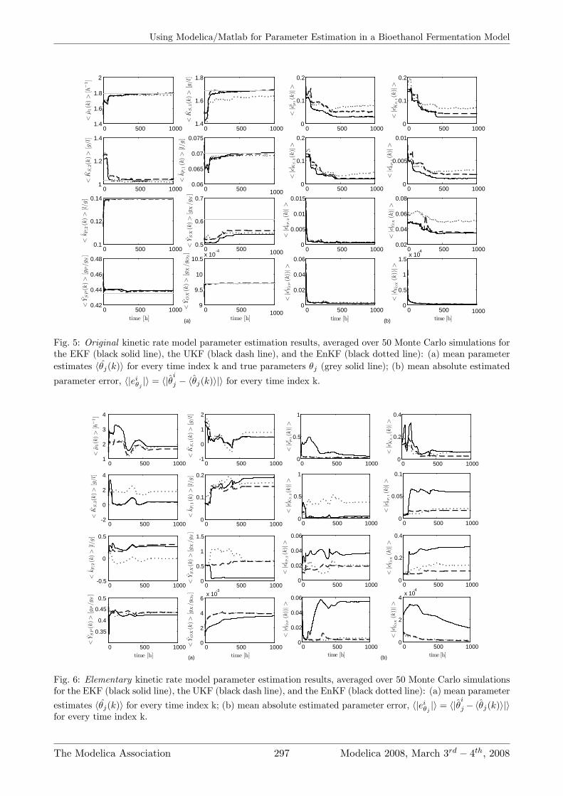
The Monte Carlo averaged performance of the es-timators using the original reaction rate model isshown in Fig. 5. The averaged estimated parame-ters h�j (k)i converge to the true parameters forall the parameters except for the slightly biasedYSP estimate and the more biased YSX estimate.In Fig. 5 column (b), the averaged estimated pa-rameter errors for the parameters fkP;2; YSP; YO2gconverge at a faster rate than for the other esti-mated parameters f�1; KS;1; KS;2; kP;1; YSXg: TheEKF and the UKF have comparable averaged es-timated parameters, while the EnKF has slightlybiased averaged estimated parameters. The bestperformance wrt. the averaged absolute estimatedparameter error hjei�j (k) ji is achieved for the EKFfollowed by the UKF and the EnKF.

The Monte Carlo averaged performance of the es-timators using the elementary reaction rate modelis shown in Fig. 6. It can be seen that the av-eraged estimated parameters no longer convergeto the true parameters of the original rate modelused in the system model simulations. It is tobe expected that some of the parameters will betime-varying to compensate for the di¤erent ki-netic rates (between the system and the estimatorkinetic rate models) and, in this way, keep a goodstate estimation performance besides their di¤er-ences. For this case, the averaged estimated para-meters h�j (k)i are considered as an unbiased esti-mate of the true (possibly time-varying) parame-ters. The averaged estimated parameters h�j (k)itake di¤erent shapes over time depending on thespeci�c estimator evaluated. In Fig. 6 column (b),the averaged absolute estimated parameter errorshjei�j (k) ji for the parameters fkP;1; kP;2; YSX; YSPgand the EKF diverge while the UKF achieves thebest performance followed by the EnKF. It is thenreasonable to consider that the averaged estimatedparameters h�j (k)i that correspond to the UKFare the best estimate of the true parameters �j (k)for this estimator reaction rate model.

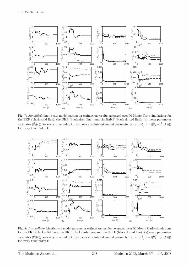
The Monte Carlo averaged performance of the es-timators using the simpli�ed reaction rate modelis shown in Fig. 7. As for the elementary case, theaveraged estimated parameters h�j (k)i are con-sidered as an unbiased estimate of the true (possi-bly time-varying) parameters. The averaged es-

timated parameters h�j (k)i have similar valuesfor the EKF and the UKF and slightly di¤erentfor the EnKF. In Fig. 7 column (b), the low-est averaged absolute estimated parameter errorshjei�j (k) ji are achieved for the EKF, closely fol-lowed by the UKF performance. For all the esti-mators the averaged absolute estimated parametererrors decrease over time.The Monte Carlo averaged performance of theestimators using the intracellular reaction ratemodel is shown in Fig. 8. As for the elementaryand simpli�ed cases, the averaged estimated para-meters h�j (k)i are considered as an unbiased esti-mate of the true (possibly time-varying) parame-ters. The averaged estimated parameters h�j (k)ihave similar values for the EKF and the UKF andslightly di¤erent for the EnKF. In Fig. 8 column(b), the averaged absolute estimated parametererrors hjei�j (k) ji decrease over time for all the pa-rameters and estimators, except for the estimatedparameter YSX with the EnKF.In Table 7 the di¤erent reaction rate models areevaluated for each �lter using the normalizedmean RMSE de�ned as

RMSE (x) =Pnx

j

Pnsimuli

2

sPntk (xj(k)�xtruej

(k))2

nt

max(xtruej )�min(xtruej )

Tab. 7: Normalized mean RMSE for the estimatedstate x and parameter � vectors .The best results forevery case is indicated by parentheses.

RMSE (:) EKF UKF EnKFOriginal x 9.11E-2 9.13E-2 (8.44E-2)

� (1.22) 1.74 1.95

Elementary x 2.09E-1 1.00E-1 (9.35E-2)� 5.57E-1 (2.73E-1) 7.54E-1

Simpli�ed x 8.36E-2 (8.05E-2) 8.77E-2� (3.21E-1) 3.56E-1 3.28E-1

Intracellular x 8.94E-2 1.05E-1 (8.60E-2)� (3.98E-1) 5.69E-1 4.71E-1

5 Conclusions

The recursive parameter estimation problem is an-alyzed for an ethanol fermentation process withdi¤erent reaction rate models. The model is im-plemented in Modelica and three nonlinear esti-mators are evaluated using the compiled Modelicamodel (Dymosim) with Matlab. Implementationdetails (e.g. how to calculate Jacobians, de�nednoise inputs, etc.) are presented.Some relevant model parameters are estimated us-ing the EKF, the UKF, and the EnKF from sim-



(a)

0 500 10001.4

1.6

1.8

<K

S;1

(k)>

[g=l

]0 500 1000

0.06

0.065

0.07

0.075

<k P

;1(k

)>

[l=g]

0 500 10000.5

0.6

0.7

<Y

SX

(k)>

[gX

=g S

]

0 500 10009

9.5

10

10.5x 10

4

time [h]

<Y

OX

(k)>

[gX

=gO

2]

0 500 10001.4

1.6

1.8

2<

¹1(k

)>

[h¡

1]

0 500 10001

1.2

1.4

<K

S;2

(k)>

[g=l

]

0 500 10000.1

0.12

0.14

<k P

;2(k

)>

[l=g]

0 500 10000.42

0.44

0.46

0.48

time [h]

<Y

SP

(k)>

[gP

=g S

]

0 500 10000

0.1

0.2

<jei K

S;1(k

)j>

0 500 10000

0.005

0.01

<jei k

P;1(k

)j>

0 500 10000.02

0.04

0.06

0.08

<jei Y

SX

(k)j

>

time [h]

0 500 10000

0.5

1

1.5x 10

4

time [h]

<jei Y

OX

(k))

j>

(b)

0 500 10000

0.1

0.2

<jei ¹

1(k

)j>

0 500 10000

0.1

0.2

<jei K

S;2(k

)j>

0 500 10000

0.005

0.01

0.015

<jei k

P;2(k

)j>

0 500 10000

0.02

0.04

0.06

<jei Y

SP

(k))

j>

Fig. 5: Original kinetic rate model parameter estimation results, averaged over 50 Monte Carlo simulations forthe EKF (black solid line), the UKF (black dash line), and the EnKF (black dotted line): (a) mean parameterestimates h�j(k)i for every time index k and true parameters �j (grey solid line); (b) mean absolute estimatedparameter error, hjei�j ji = hj�

i

j � h�j(k)iji for every time index k.

0 500 10001

2

3

4

<¹

1(k

)>

[h¡

1]

0 500 10002

0

2

4

<K

S;2

(k)>

[g=l

]

0 500 10000.5

0

0.5

<k P

;2(k

)>

[l=g]

0 500 1000

0.35

0.4

0.45

0.5

time [h]

<Y

SP

(k)>

[gP

=gS

]

0 500 10001

0

1

2

<K

S;1

(k)>

[g=l

]

0 500 10000

0.1

0.2

<k P

;1(k

)>

[l=g]

0 500 10000

0.5

1

1.5

<Y

SX

(k)>

[gX

=g S

]

0 500 10000

2

4

6x 10

3

time [h]

<Y

OX

(k)>

[gX

=g O

2]

0 500 10000

0.5

1

<jei K

S;2(k

)j>

0 500 10000

0.02

0.04

0.06

<jei k

P;2(k

)j>

0 500 10000

0.02

0.04

0.06

time [h]

<jei Y

SP

(k))

j>

0 500 10000

0.5

1

<jei ¹

1(k

)j>

0 500 10000

0.05

0.1

<jei k

P;1(k

)j>

0 500 10000

0.2

0.4

<jei Y

SX

(k)j

>

0 500 10000

2

4x 10

4

time [h]

<jei Y

OX

(k))

j>

0 500 10000

0.2

0.4

<jei K

S;1(k

)j>

(a) (b)

Fig. 6: Elementary kinetic rate model parameter estimation results, averaged over 50 Monte Carlo simulationsfor the EKF (black solid line), the UKF (black dash line), and the EnKF (black dotted line): (a) mean parameter

estimates h�j(k)i for every time index k; (b) mean absolute estimated parameter error, hjei�j ji = hj�i

j �h�j(k)ijifor every time index k.



0 500 10000

1

2

3<

¹1(k

)>

[h¡

1]

0 500 10000.5

1

1.5

2

<K

S;1

(k)>

[g=l

]0 500 1000

1

0

1

2

<K

S;2

(k)>

[g=l

]

0 500 10000

0.05

0.1

<k P

;1(k

)>

[l=g

]

0 500 10000.1

0.12

0.14

0.16

<k P

;2(k

)>

[l=g]

0 500 10000.4

0.6

0.8

1

<Y

SX

(k)>

[gX

=g S

]

0 500 10000.4

0.45

0.5

time [h]

<Y

SP

(k)>

[gP

=g S

]

0 500 10000.9

1

1.1x 10

3

time [h]

<Y

OX

(k)>

[gX

=gO

2]

0 500 10000

0.1

0.2

<jei ¹

1(k

)j>

0 500 10000

0.1

0.2

<jei K

S;2(k

)j>

0 500 10000

0.005

0.01

0.015

<jei k

P;2(k

)j>

0 500 10000

0.02

0.04

0.06

time [h]

<jei Y

SP

(k))

j>

0 500 10000

0.1

0.2

<jei K

S;1(k

)j>

0 500 10004

6

8

10x 10

3

<jei k

P;1(k

)j>

0 500 10000.02

0.04

0.06

0.08

<jei Y

SX

(k)j

>

0 500 10000

0.5

1

1.5x 10

4

time [h]

<jei Y

OX

(k))

j>

(a) (b)

Fig. 7: Simpli�ed kinetic rate model parameter estimation results, averaged over 50 Monte Carlo simulations forthe EKF (black solid line), the UKF (black dash line), and the EnKF (black dotted line): (a) mean parameter



0 500 10000

0.1

0.2

<jei ¹

1(k

)j>

0 500 10000

0.1

0.2

<jei K

S;1(k

)j>

0 500 10000

0.1

0.2

<jei K

S;2(k

)j>

0 500 10000

0.005

0.01

<jei k

P;1(k

)j>

0 500 10000

0.005

0.01

0.015

<jei k

P;2(k

)j>

0 500 10000.02

0.04

0.06

0.08

<jei Y

SX

(k)j

>

0 500 10000

0.02

0.04

0.06

time [h]

<jei Y

SP

(k))

j>

0 500 10000

0.5

1x 10

4

time [h]

<jei Y

OX

(k))

j>

0 500 10001

2

3

<¹

1(k

)>

[h¡

1]

0 500 10001

1.5

2

2.5

<K

S;1

(k)>

[g=l

]

0 500 10000.5

1

1.5

<K

S;2

(k)>

[g=l

]

0 500 10000.05

0.1

0.15

0.2

<k P

;1(k

)>

[l=g]

0 500 10000.1

0.15

0.2

<k P

;2(k

)>

[l=g]

0 500 10000.4

0.6

0.8

1

<Y

SX

(k)>

[gX

=g S

]

0 500 10000.4

0.45

0.5

time [h]

<Y

SP

(k)>

[gP

=g S

]

0 500 10009

9.5

10

10.5x 104

time [h]

<Y

OX

(k)>

[gX

=g O

2]

(a) (b)

Fig. 8: Intracellular kinetic rate model parameter estimation results, averaged over 50 Monte Carlo simulationsfor the EKF (black solid line), the UKF (black dash line), and the EnKF (black dotted line): (a) mean parameter





ulated data sets over 50 Monte Carlo simulations.Four di¤erent reaction rate models are used by theestimators while the simulated data sets are gen-erated assuming that the original reaction rateparameters have been estimated experimentally.When using the original reaction rate model inthe estimator, the best parameter estimation isachieved by the EKF with slightly poorer perfor-mances for the UKF and the EnKF. The lowerperformance of the UKF can be explained by thelack of tunig of its parameters. For the estimatorusing the elementary reaction rate model, the bestparameter estimation corresponds to the UKF,while the EnKF has a poorer performance and theEKF diverges for some of the parameters. For theestimator with the simpli�ed reaction rate modelsimilar performances are achieved for the 3 esti-mators; the UKF slightly outperforms the othertwo. For the estimator with the intracellular re-action rate model, the best parameter estimationperformance corresponds to the EKF.The EnKF has a poor parameter estimation per-formance for most of the cases but when consid-ering the mean RMSE of the estimated states itoutperforms the other estimators for three of thefour cases (see Table 7).The computational cost of the estimators increasesconsiderably from the EKF to the EnKF becauseof the number of projections required for everyestimator iteration. The fermentation model isrun from a Dymosim executable �le and this slowsdown the computational performance of the esti-mators (i.e. the computational time required forevery estimator interation) mainly because Dy-mosim uses a slow �le input/output interface. De-spite this practical disadvantage, nonlinear esti-mators can be evaluated with complex Modelicamodels in a simple way. Our future work will focuson the parameter identi�ability of the completemodel.

References

[1] P. S. Agachi, Z. K. Cristea, and A. Imre-Lucaci,Model Based Control. Case Studies in ProcessEngineering. Weinheim: Wiley-VCH VerlagGmbH&Co., 2006.

[2] B. Lie and J. I. Videla, �Continuous bioethanolproduction by fermentation,� in Green Energywith energy management and IT, Stockholm,2008.

[3] P. M. Doran, Bioprocess Engineering Principles.San Diego: Academic Press, 1995.

[4] J. L. Crassidis and J. L. Junkins, Optimal estima-tion of dynamic systems, ser. CRC applied math-ematics and nonlinear science series. Chapman& Hall, 2000.

[5] S. F. Schmidt, Application of State-Space Methodsto Navigation Problems, c.t. leondes ed. Aca-demic Press, New York, San Francisco, London,1966, vol. 3, pp. 293�340.

[6] R. E. Kalman, �A new approach to linear �lter-ing and prediction problems,�Transactions of theASME�Journal of Basic Engineering, vol. 82, no.Series D, pp. 35�45, 1960.

[7] D. Simon, Optimal State Estimation � Kalman,H1, and Nonlinear Approaches. Hoboken, NewJersey: John Wiley & Sons, Inc., 2006.

[8] S. J. Julier, J. K. Uhlmann, and H. F. Durrant-Whyte, �A new approach for �ltering nonlinearsystems,� in Proceedings of the 1995 AmericanControl Conference, Seattle, WA, 1995, pp. 1628�1632.

[9] S. Julier and J. Uhlmann, �A general method forapproximating nonlinear transformations of prob-ability distributions,� tech. rep., RRG, Dept. ofEngineering Science, University of Oxford, Nov1996, Tech. Rep., 1996.

[10] � � , �A new extension of the Kalman �l-ter to nonlinear systems,� in Int. Symp.Aerospace/Defense Sensing, Simul. and Controls,Orlando, FL, 1997.

[11] S. J. Julier and J. K. Uhlmann, �Unscented �l-tering and nonlinear estimation (invited paper),�in Proceedings of the IEEE, vol. 92(3). IEEEInstitute of Electrical and Electronics, 2004, pp.401�422.

[12] G. Evensen, �The ensemble kalman �lter: The-oretical formulation and practical implementa-tion,� Ocean Dynamics, vol. 53, pp. 343�367,2003.

[13] S. Gillijns, O. B. Mendoza, J. Chandrasekar, B. L.R. D. Moor, D. S. Bernstein, and A. Ridley,�What is the ensemble kalman �lter and how welldoes it work?� in Proceedings of the 2006 Ameri-can Control Conference, Minneapolis, Minnesota,USA, June 2006.



Using Modelica/Matlab for parameter estimation in a ... · Using Modelica/Matlab for parameter...

Documents

Transcript of Using Modelica/Matlab for parameter estimation in a ... · Using Modelica/Matlab for parameter...