Parameter Estimation in a Moving Horizon...
32
Parameter Estimation in a Moving Horizon Perspective State and Parameter Estimation in Dynamical Systems Lennart Ljung Reglerteknik, ISY, Linköpings Universitet Lennart Ljung Parameter Estimation in a Moving Horizon Perspective AUTOMATIC CONTROL REGLERTEKNIK LINKÖPINGS UNIVERSITET
Transcript of Parameter Estimation in a Moving Horizon...
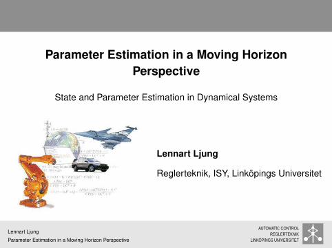
Parameter Estimation in a Moving HorizonPerspective
State and Parameter Estimation in Dynamical Systems
Lennart Ljung
Reglerteknik, ISY, Linköpings Universitet
Lennart Ljung
Parameter Estimation in a Moving Horizon Perspective
AUTOMATIC CONTROLREGLERTEKNIK
LINKÖPINGS UNIVERSITET

State and Parameter Estimation in Dynamical Systems
OUTLINE1Problem Formulation
2State Estimation with Sparse Process Disturbances in Linear Systems
3Parameter and State Estimation in Unknown (Linear) Systems
Lennart Ljung
Parameter Estimation in a Moving Horizon Perspective
AUTOMATIC CONTROLREGLERTEKNIK
LINKÖPINGS UNIVERSITET
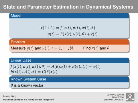
State and Parameter Estimation in Dynamical Systems
Model
x(t + 1) = f (x(t), u(t), w(t), θ)
y(t) = h(x(t), u(t), θ) + e(t)
Problem
Measure y(t) and u(t), t = 1, . . . , N. Find x(t) and θ
Linear Case
f (x(t), u(t), w(t), θ) = A(θ)x(t) + B(θ)u(t) + w(t)h(x(t), u(t), θ) = C(θ)x(t)
Known System Case
θ is a known vector
Lennart Ljung
Parameter Estimation in a Moving Horizon Perspective
AUTOMATIC CONTROLREGLERTEKNIK
LINKÖPINGS UNIVERSITET

Maximum Likelihood
View Θ = [θ, x(t), t = 1, . . . , N] as unknown parameters. Assumee(t) ∈ N(0, I). Then the negative log-likelihood function is
V(θ, x(·)) =N
∑t=1‖y(t)− h(x(t), u(t), θ)‖2
Too many parameters! ⇒ Regularize!
Lennart Ljung
Parameter Estimation in a Moving Horizon Perspective
AUTOMATIC CONTROLREGLERTEKNIK
LINKÖPINGS UNIVERSITET
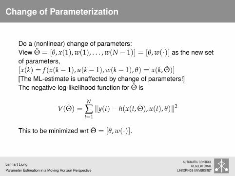
Change of Parameterization
Do a (nonlinear) change of parameters:View Θ̃ = [θ, x(1), w(1), . . . , w(N− 1)] = [θ, w(·)] as the new setof parameters,[x(k) = f (x(k− 1), u(k− 1), w(k− 1), θ) = x(k, Θ̃)][The ML-estimate is unaffected by change of parameters!]The negative log-likelihood function for Θ̃ is
V(Θ̃) =N
∑t=1‖y(t)− h(x(t, Θ̃), u(t), θ)‖2
This to be minimized wrt Θ̃ = [θ, w(·)].
Lennart Ljung
Parameter Estimation in a Moving Horizon Perspective
AUTOMATIC CONTROLREGLERTEKNIK
LINKÖPINGS UNIVERSITET
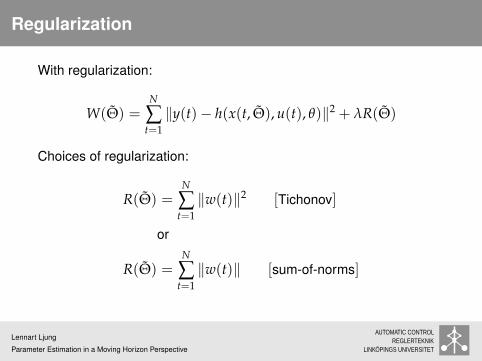
Regularization
With regularization:
W(Θ̃) =N
∑t=1‖y(t)− h(x(t, Θ̃), u(t), θ)‖2 + λR(Θ̃)
Choices of regularization:
R(Θ̃) =N
∑t=1‖w(t)‖2 [Tichonov]
or
R(Θ̃) =N
∑t=1‖w(t)‖ [sum-of-norms]
Lennart Ljung
Parameter Estimation in a Moving Horizon Perspective
AUTOMATIC CONTROLREGLERTEKNIK
LINKÖPINGS UNIVERSITET

Classical Interpretation
Regularization curbs the flexibility of (large) model sets by pulling theparameters toward the origin.
Tichonov: Regularization for Bias-Variance Trade-off
Sum-of-norms: Regularization for Sparsity:Solutions with “many” ‖w(t)‖ = 0 are favored
Lennart Ljung
Parameter Estimation in a Moving Horizon Perspective
AUTOMATIC CONTROLREGLERTEKNIK
LINKÖPINGS UNIVERSITET

Bayesian Interpretation
Suppose w(t) ∈ N(0, I) and θ is a random vector with θ ∈ N(0, cI)(dim = d). Then the joint pdf of θ, y(·), w(·) is
−2 log P(y(·), w(·), θ) ∼N
∑t=1
[‖y(t)− h(x(t, w(·)), u(t), θ)‖2 + ‖w(t)‖2]
+ ‖θ‖2/c + constx(t, w(·)) = f (x(t− 1, w(·)), u(t− 1), w(t− 1), θ)
so the MAP estimate of Θ̃ is
ˆ̃Θ = arg min W(Θ̃) + ‖θ‖2/c
which for c→ ∞ is the same as the Tichonov-regularized MLestimate of Θ̃.
Lennart Ljung
Parameter Estimation in a Moving Horizon Perspective
AUTOMATIC CONTROLREGLERTEKNIK
LINKÖPINGS UNIVERSITET

Outline
2State Estimation with Sparse Process Disturbances in Linear Systems
3Parameter and State Estimation in Unknown (Linear) Systems
Lennart Ljung
Parameter Estimation in a Moving Horizon Perspective
AUTOMATIC CONTROLREGLERTEKNIK
LINKÖPINGS UNIVERSITET
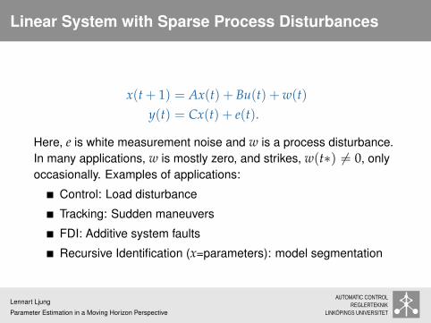
Linear System with Sparse Process Disturbances
x(t + 1) = Ax(t) + Bu(t) + w(t)y(t) = Cx(t) + e(t).
Here, e is white measurement noise and w is a process disturbance.In many applications, w is mostly zero, and strikes, w(t∗) 6= 0, onlyoccasionally. Examples of applications:
Control: Load disturbance
Tracking: Sudden maneuvers
FDI: Additive system faults
Recursive Identification (x=parameters): model segmentation
Lennart Ljung
Parameter Estimation in a Moving Horizon Perspective
AUTOMATIC CONTROLREGLERTEKNIK
LINKÖPINGS UNIVERSITET
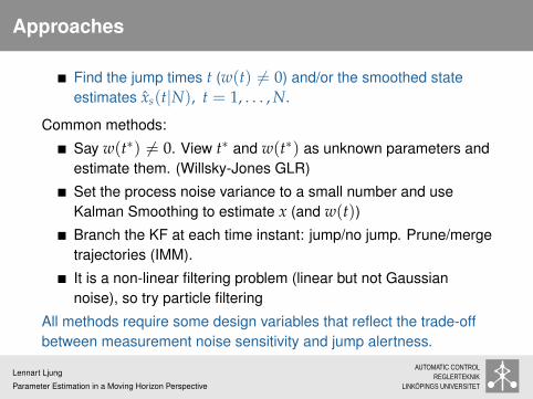
Approaches
Find the jump times t (w(t) 6= 0) and/or the smoothed stateestimates x̂s(t|N), t = 1, . . . , N.
Common methods:
Say w(t∗) 6= 0. View t∗ and w(t∗) as unknown parameters andestimate them. (Willsky-Jones GLR)
Set the process noise variance to a small number and useKalman Smoothing to estimate x (and w(t))Branch the KF at each time instant: jump/no jump. Prune/mergetrajectories (IMM).
It is a non-linear filtering problem (linear but not Gaussiannoise), so try particle filtering
All methods require some design variables that reflect the trade-offbetween measurement noise sensitivity and jump alertness.
Lennart Ljung
Parameter Estimation in a Moving Horizon Perspective
AUTOMATIC CONTROLREGLERTEKNIK
LINKÖPINGS UNIVERSITET
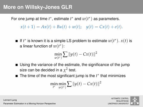
More on Willsky-Jones GLR
For one jump at time t∗, estimate t∗ and w(t∗) as parameters.
x(t + 1) = Ax(t) + Bu(t) + w(t); y(t) = Cx(t) + e(t).
If t∗ is known it is a simple LS problem to estimate w(t∗). x(t) isa linear function of w(t∗):
minw(t∗)
∑ ‖y(t)− Cx(t)‖2
Using the variance of the estimate, the significance of the jumpsize can be decided in a χ2 test.The time of the most significant jump is the t∗ that minimizes
mint∗
minw(t∗)
∑ ‖y(t)− Cx(t)‖2
Lennart Ljung
Parameter Estimation in a Moving Horizon Perspective
AUTOMATIC CONTROLREGLERTEKNIK
LINKÖPINGS UNIVERSITET
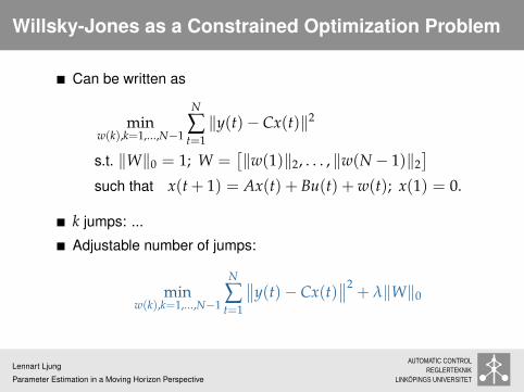
Willsky-Jones as a Constrained Optimization Problem
Can be written as
minw(k),k=1,...,N−1
N
∑t=1‖y(t)− Cx(t)‖2
s.t. ‖W‖0 = 1; W =[‖w(1)‖2, . . . , ‖w(N− 1)‖2
]such that x(t + 1) = Ax(t) + Bu(t) + w(t); x(1) = 0.
k jumps: ...
Adjustable number of jumps:
minw(k),k=1,...,N−1
N
∑t=1
∥∥y(t)− Cx(t)∥∥2
+ λ‖W‖0
Lennart Ljung
Parameter Estimation in a Moving Horizon Perspective
AUTOMATIC CONTROLREGLERTEKNIK
LINKÖPINGS UNIVERSITET

Do the `1 Trick! (`0 → `1)
This problem is computationally forbidding, so relax the `0 norm:
minw(k),k=1,...,N−1
N
∑t=1
∥∥y(t)− Cx(t)∥∥2
+ λ‖W‖1
= minw(k),k=1,...,N−1
N
∑t=1
∥∥y(t)− Cx(t)∥∥2
+ λN
∑t=1‖w(t)‖2
[StateSON] This is our Moving Horizon State estimation problem withSON-regularization.Choice of λ : ....Ohlsson, Gustafsson, Ljung, Boyd: Smoothed state estimates underabrupt changes using sum-of-norms regularization. Automatica48(4):595-605, April 2012
Lennart Ljung
Parameter Estimation in a Moving Horizon Perspective
AUTOMATIC CONTROLREGLERTEKNIK
LINKÖPINGS UNIVERSITET

How Does it Work?
DC motor with impulse disturbances at t = 49, 55State RMSE over 500 realizations as a function of time t : 0→ 100.Dashed blue: Willsky-Jones, Solid green: StateSON
0 20 40 60 80 1000
0.5
1
1.5
2
2.5
Lennart Ljung
Parameter Estimation in a Moving Horizon Perspective
AUTOMATIC CONTROLREGLERTEKNIK
LINKÖPINGS UNIVERSITET
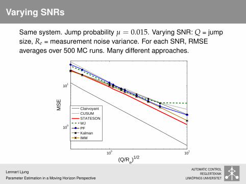
Varying SNRs
Same system. Jump probability µ = 0.015. Varying SNR: Q = jumpsize, Re = measurement noise variance. For each SNR, RMSEaverages over 500 MC runs. Many different approaches.
100
101
100
101
(Q/Re)1/2
MS
E
ClairvoyantCUSUMSTATESONWJPFKalmanIMM
Lennart Ljung
Parameter Estimation in a Moving Horizon Perspective
AUTOMATIC CONTROLREGLERTEKNIK
LINKÖPINGS UNIVERSITET

Conclusions Sparse State Estimation
Solving the (moving horizon) state estimation problem withSum-of-Norm (`1) regularization is a good way to handle sparseprocess noise.
Performance is at least as good as for more complicated(hypothesis-testing) routines
Lennart Ljung
Parameter Estimation in a Moving Horizon Perspective
AUTOMATIC CONTROLREGLERTEKNIK
LINKÖPINGS UNIVERSITET
State and Parameter Estimation
New problem: No longer assume that the parameter vector is known.
How to estimate also the parameter θ in the system description?
Lennart Ljung
Parameter Estimation in a Moving Horizon Perspective
AUTOMATIC CONTROLREGLERTEKNIK
LINKÖPINGS UNIVERSITET
State and Parameter Estimation
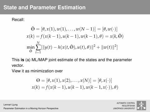
Recall:
Θ̃ = [θ, x(1), w(1), . . . , w(N− 1)] = [θ, w(·)]x(k) = f (x(k− 1), u(k− 1), w(k− 1), θ) = x(k, Θ̃)
minΘ̃
N
∑t=1
[‖y(t)− h(x(t, Θ̃), u(t), θ)‖2 + ‖w(t)‖2]
This is (a) ML/MAP joint estimate of the states and the parametervector.View it as minimization over
Θ = [θ, x(1), x(2), . . . , x(N)] = [θ, x(·)]x(k) = f (x(k− 1), u(k− 1), w(k− 1, x(·)), θ)
Lennart Ljung
Parameter Estimation in a Moving Horizon Perspective
AUTOMATIC CONTROLREGLERTEKNIK
LINKÖPINGS UNIVERSITET
Joint State and Parameter Estimate
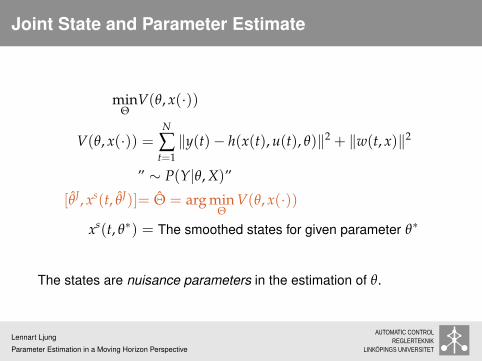
minΘ
V(θ, x(·))
V(θ, x(·)) =N
∑t=1‖y(t)− h(x(t), u(t), θ)‖2 + ‖w(t, x)‖2
” ∼ P(Y|θ, X)”
[θ̂J, xs(t, θ̂J)]= Θ̂ = arg minΘ
V(θ, x(·))
xs(t, θ∗) = The smoothed states for given parameter θ∗
The states are nuisance parameters in the estimation of θ.
Lennart Ljung
Parameter Estimation in a Moving Horizon Perspective
AUTOMATIC CONTROLREGLERTEKNIK
LINKÖPINGS UNIVERSITET

Possible Parameter Estimates
θ̂Jas above; joint estimate with states
θ̂ML = arg max P(Y|θ) ∼ arg max∫
P(Y|θ, X)P(X|θ)dX
θ̂SEM = arg minθ
N
∑t=1‖y(t)− h(xs(t, θ), u(t), θ)‖2 "smoothing error est"
θ̂J is conceptually simple to compute (in line with MPC) - couldbe a lot of numerical work, though.θ̂SEM sounds like a good idea: “Smoothing Error minimizationshould be better than Prediction Error minimization”θ̂ML has good credentials, but the ML criterion for nonlinearmodels involves solving the non-linear filtering problem.(The marginalization wrt x above is an extensive task.)
Lennart Ljung
Parameter Estimation in a Moving Horizon Perspective
AUTOMATIC CONTROLREGLERTEKNIK
LINKÖPINGS UNIVERSITET

Marginalization: Picture
The integration will of course in general affect the maximum:
Lennart Ljung
Parameter Estimation in a Moving Horizon Perspective
AUTOMATIC CONTROLREGLERTEKNIK
LINKÖPINGS UNIVERSITET

One more Estimation Method: EM
When the likelihood function is difficult to form, it may beadvantageous to extend the problem with latent variables for a welldefined likelihood function, and iterate between estimating thesevariables and the parameters.This is the EM-algorithm, and in our case the states x can serve asthese latent variables.Take expectation of V(θ, x(.)) under the assumption that x has beengenerated by the model with the parameter value α:
Q(θ, α) = E[V(θ, x(·))|Y, θ = α)]
θk = arg minθ
Q(θ, θk−1)
θ̂EM = limk→∞
θk [≈ θML?]
How much work is required to form Q(θ, α)?
Lennart Ljung
Parameter Estimation in a Moving Horizon Perspective
AUTOMATIC CONTROLREGLERTEKNIK
LINKÖPINGS UNIVERSITET

Linear Models
How are these estimates related - and are they any good?3Parameter and State Estimation in Unknown Linear Systems
Linear Model: (Joint discussions with Thomas Schön and DavidTörnqvist)
x(t + 1) = A(θ)x(t) + B(θ)u(t) + w(t)y(t) = C(θ)x(t) + e(t)
Ew(t)wT(t) = Q(θ) Ee(t)eT(t) = R(θ)
Specialize to (without much loss of generality):
u(t) ≡ 0, Q(θ) = I, R(θ) = I
Lennart Ljung
Parameter Estimation in a Moving Horizon Perspective
AUTOMATIC CONTROLREGLERTEKNIK
LINKÖPINGS UNIVERSITET
Notation
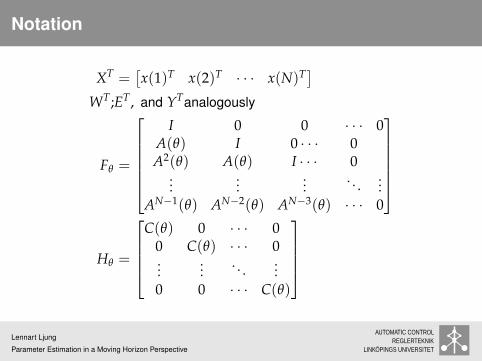
XT =[x(1)T x(2)T · · · x(N)T]
WT;ET, and YTanalogously
Fθ =
I 0 0 · · · 0
A(θ) I 0 · · · 0A2(θ) A(θ) I · · · 0
......
.... . .
...AN−1(θ) AN−2(θ) AN−3(θ) · · · 0
Hθ =
C(θ) 0 · · · 0
0 C(θ) · · · 0...
.... . .
...0 0 · · · C(θ)
Lennart Ljung
Parameter Estimation in a Moving Horizon Perspective
AUTOMATIC CONTROLREGLERTEKNIK
LINKÖPINGS UNIVERSITET

Matrix Formulation
X = FθW, Y = HθX + E
W and E are Gaussian random vectors N(0, I).
Y = HθFθW + E
Y ∈ N(0, Rθ), Rθ = HθFθFTθ HT
θ + I
−2 log P(Y|θ) = YTR−1θ Y + log det Rθ
−2 log P(Y|θ, X) = ‖Y−HθX‖2
In a Bayesian setting with θ ∈ N(0, cI)
P(Y, X, θ) = P(Y|X, θ)P(X|θ)P(θ)V(Y, X, θ) = −2 log P(Y, X, θ) = ||Y−HθX‖2 + ‖F−1
θ X‖2 + ‖θ‖2/c
Lennart Ljung
Parameter Estimation in a Moving Horizon Perspective
AUTOMATIC CONTROLREGLERTEKNIK
LINKÖPINGS UNIVERSITET
The Estimates
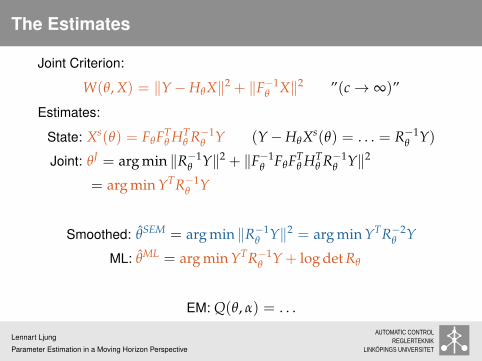
Joint Criterion:
W(θ, X) = ‖Y−HθX‖2 + ‖F−1θ X‖2 ”(c→ ∞)”
Estimates:
State: Xs(θ) = FθFTθ HT
θ R−1θ Y (Y−HθXs(θ) = . . . = R−1
θ Y)
Joint: θJ = arg min ‖R−1θ Y‖2 + ‖F−1
θ FθFTθ HT
θ R−1θ Y‖2
= arg min YTR−1θ Y
Smoothed: θ̂SEM = arg min ‖R−1θ Y‖2 = arg min YTR−2
θ Y
ML: θ̂ML = arg min YTR−1θ Y + log det Rθ
EM: Q(θ, α) = . . .
Lennart Ljung
Parameter Estimation in a Moving Horizon Perspective
AUTOMATIC CONTROLREGLERTEKNIK
LINKÖPINGS UNIVERSITET
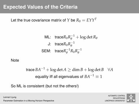
Expected Values of the Criteria
Let the true covariance matrix of Y be R0 = EYYT
ML: traceR0R−1θ + log det Rθ
J: traceR0R−1θ
SEM: traceR−1θ R0R−1
θ
Note
trace BA−1 + log det A ≥ dim B + log det B ∀A
equality iff all eigenvalues of BA−1 ≡ 1
So ML is consistent (but not the others!)
Lennart Ljung
Parameter Estimation in a Moving Horizon Perspective
AUTOMATIC CONTROLREGLERTEKNIK
LINKÖPINGS UNIVERSITET
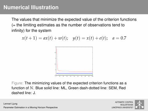
Numerical Illustration
The values that minimize the expected value of the criterion functions(= the limiting estimates as the number of observations tend toinfinity) for the system
x(t + 1) = ax(t) + w(t); y(t) = x(t) + e(t); a = 0.7
0 10 20 30 40 50 60 70 80 90 1000.5
1
1.5
2
2.5
3
Figure: The minimizing values of the expected criterion functions as afunction of N. Blue solid line: ML, Green dash-dotted line: SEM, Reddashed line: J.
Lennart Ljung
Parameter Estimation in a Moving Horizon Perspective
AUTOMATIC CONTROLREGLERTEKNIK
LINKÖPINGS UNIVERSITET
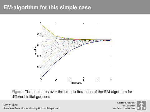
EM-algorithm for this simple case
Figure: The estimates over the first six iterations of the EM-algorithm fordifferent initial guesses
Lennart Ljung
Parameter Estimation in a Moving Horizon Perspective
AUTOMATIC CONTROLREGLERTEKNIK
LINKÖPINGS UNIVERSITET

Some Observations
J ∼ W(θ, X) ML ∼ ”∫
W(θ, X)dX”
J∼ YTR−1θ Y ML ∼ YTR−1
θ Y + log det Rθ
J is not consistent,(but ML is, of course)
J and ML are different maxima of W(θ, X)
The marginalization of W(θ, X) only leads to adata-independent (regularization) term log det Rθ
Is a similar result true also in the non-linear case?
How would EM work in the non-linear case? (Schön, Wills,Ninness: Automatica 2011.)
Lennart Ljung
Parameter Estimation in a Moving Horizon Perspective
AUTOMATIC CONTROLREGLERTEKNIK
LINKÖPINGS UNIVERSITET
Conclusions: State and Parameter Estimation
Tempting to use MPC-thinking for model estimation usingMoving Horizon Estimation - “Just” minimize over θ as well.
This however leads to inconsistent estimates.
Can it be saved by thoughtful regularization?
Lennart Ljung
Parameter Estimation in a Moving Horizon Perspective
AUTOMATIC CONTROLREGLERTEKNIK
LINKÖPINGS UNIVERSITET