ORIGINS OF ANALYSIS METHODS IN ENERGY SIMULATION PROGRAMS

USED FOR HIGH PERFORMANCE COMMERCIAL BUILDINGS

A Thesis

by

SUKJOON OH

Submitted to the Office of Graduate Studies of

Texas A&M University

in partial fulfillment of the requirements for the degree of

MASTER OF SCIENCE

Chair of Committee, Jeff S. Haberl

Committee Members, David E. Claridge

Charles H. Culp

Jonathan C. Coopersmith

Head of Department, Ward V. Wells

August 2013

Major Subject: Architecture

Copyright 2013

ii

ABSTRACT

Current designs of high performance buildings utilize hourly building energy

simulations of complex, interacting systems. Such simulations need to quantify the

benefits of numerous features including: thermal mass, HVAC systems and, in some

cases, special features such as active and passive solar systems, photovoltaic systems,

and lighting and daylighting systems. Unfortunately, many high performance buildings

today do not perform the way they were simulated. One potential reason for this

discrepancy is that designers using the simulation programs do not understand the

analysis methods that the programs are based on and therefore they may have

unreasonable expectations about the system performance or use.

The purpose of this study is to trace the origins of a variety of simulation

programs and the analysis methods used in the programs to analyze high performance

buildings in the United States. Such an analysis is important to better understand the

capabilities of the simulation programs so they can be used more accurately to simulate

the performance of an intended design. The goal of this study is to help explain the

origins of the analysis methods used in whole-building energy simulation, solar system

analysis simulation or design, and lighting and daylighting analysis simulation programs.

A comprehensive history diagram or genealogy chart, which resolves discrepancies

between the diagrams of previous studies, has been provided to support the explanations

for the above mentioned simulation programs.

iii

DEDICATION

To

My Loving God, Wife and Family

iv

ACKNOWLEDGEMENTS

First of all, I would like to sincerely thank my loving God for the guidance

throughout the course of my life, including this research.

I would like to express my deepest appreciation to the committee chair, Dr. Jeff

S. Haberl. I really appreciate your expertise and support throughout the course of this

research. I would like to thank my committee members, Dr. David E. Claridge, Dr.

Charles H. Culp, and Dr. Jonathan C. Coopersmith for your encouragement and insights.

My thanks go to the reviewers for the genealogy chart in this study: Zulfikar O.

Cumali, Dr. Edward F. Sowell, Dennis R. Landsberg, Prof. Larry O. Degelman, Dr.

Daniel E. Fisher, Dr. Juan-Carlos Baltazar-Cervantes, and Dr. Richard R. Perez. I really

appreciate your time and useful comments. I also appreciate Dr. Mohsen Farzad and

Mick Schwedler’s information about Carrier’s HAP program and Trane’s TRACE

program.

My thanks also go to the copyright holders: American Society of Heating,

Refrigerating and Air-Conditioning Engineers (ASHRAE), American Concrete Institute

(ACI), Brad Grantham, Electric Power Research Institute (EPRI), Energy Systems

Laboratory (ESL) at Texas A&M University, John Wiley & Sons, Inc., Lawrence

Berkeley National Laboratory (LBNL), Rocky Mountain Institute (RMI), Springer, the

University of Illinois at Urbana-Champaign (UIUC). Using your materials will help my

readers better understand this study.

v

I would like to recognize my friends and colleagues, especially for Chunliu Mao

and Sandeep Kota, who are graduate assistant researchers at the ESL. Thank you for

making this study rigorous.

Finally, thanks to my loving mother, father, sister and sister’s family, and my

wife’s family for your best encouragement. I really thank my wife, Soo Jeoung Han, for

your beautiful patience and love.

vi

TABLE OF CONTENTS

Page

ABSTRACT .......................................................................................................................ii

DEDICATION ................................................................................................................. iii

ACKNOWLEDGEMENTS .............................................................................................. iv

TABLE OF CONTENTS .................................................................................................. vi

LIST OF FIGURES ............................................................................................................ x

LIST OF TABLES ...........................................................................................................xii

CHAPTER I INTRODUCTION ....................................................................................... 1

1.1 Background ...................................................................................................... 1 1.2 Objectives and Scope ....................................................................................... 2 1.3 Significance of the Study ................................................................................. 3

1.4 Limitations of the Study ................................................................................... 4 1.5 Organization of the Thesis ............................................................................... 5

CHAPTER II LITERATURE REVIEW ........................................................................... 6

2.1 Defining High Performance Buildings ............................................................. 6

2.2 Review of Previous Attempts to Trace the Methods Used in Simulation

Programs and the History of Simulation Programs ........................................ 10

2.2.1 Proceedings of the first symposium on use of computers for

environmental engineering related to buildings

(Kusuda ed., 1971) .......................................................................... 13 2.2.2 Building energy analysis computer programs with

solar heating and cooling system capabilities

(Feldman and Merriam, 1979) ........................................................ 14 2.2.3 Proceedings of the building energy simulation conference

(US DOE, 1985) .............................................................................. 16 2.2.4 A bibliography of available computer programs in the area of

heating, ventilating, air conditioning, and refrigeration

(Degelman and Andrade, 1986) ...................................................... 17

vii

2.2.5 An annotated guide to models and algorithms for energy

calculations relating to HVAC equipment (Yuill, 1990) and

annotated guide to load calculation models and algorithms

(Spitler, 1996) .................................................................................. 18

2.2.6 Historical development of building energy calculations

(Ayres and Stamper, 1995) .............................................................. 20 2.2.7 Evolution of building energy simulation methodology

(Sowell and Hittle, 1995) ................................................................ 22 2.2.8 Short-time-step analysis and simulation of homes and

buildings during the last 100 years (Shavit, 1995) .......................... 24 2.2.9 Early history and future prospects of buildings system

simulation (Kusuda, 1999) .............................................................. 27

2.2.10 Literature review of uncertainty of analysis methods

(F-Chart, PV F-Chart , and DOE-2 program)

(Haberl and Cho, 2004a, 2004b, 2004c) ......................................... 28

2.2.11 Contrasting the capabilities of building energy performance

simulation programs (Crawley et al., 2005) .................................... 33

2.2.12 Historical survey of daylighting calculation methods and

their use in energy performance simulation

(Kota and Haberl, 2009) .................................................................. 34

2.2.13 Pre-read for Building Energy Modeling (BEM) innovation

summit (Tupper et al., 2011) ........................................................... 35

2.3 Summary of Literature Review ...................................................................... 39

CHAPTER III METHODOLOGY .................................................................................. 49

3.1 Overview of Methodology ............................................................................. 49 3.2 Identification of Major Groups of Simulation Programs ............................... 51

3.2.1 Whole-building energy simulation programs .................................. 54 3.2.2 Solar energy simulation programs ................................................... 55 3.2.3 Lighting and daylighting simulation program ................................. 56

3.2.4 Scope and summary table of each simulation program ................... 57 3.3 Review of Each Group of the Simulation Programs by Tracing

the Origins of the Analysis Methods Used in the Simulation Programs ........ 63 3.4 Development of a New Comprehensive History Diagram ............................. 64

3.4.1 Identify the analysis methods used in the simulation programs ...... 64 3.4.2 Accurately analyze the historical facts of the previous studies ....... 66

3.4.3 Add relevant historical information about the analysis methods

to identify from where the analysis methods originated ................. 67 3.5 Review of the New Comprehensive Genealogy Chart by Key Experts of

Each Program Group ...................................................................................... 67 3.6 Presentation and Analysis of the New Comprehensive History Diagram

(Genealogy Chart) .......................................................................................... 68 3.6.1 Discuss the new simulation genealogy chart by time period .......... 68

viii

3.6.2 Discuss the new simulation genealogy chart by tracing specific

analysis method ............................................................................... 69 3.6.3 Discuss the new simulation genealogy chart by tracing specific

simulation programs ........................................................................ 69

3.6.4 Discuss the new simulation genealogy chart by tracing the

influence of specific organizations or support funding ................... 69 3.7 Summary of Methodology ............................................................................. 69

CHAPTER IV RESULTS ............................................................................................... 71

4.1 Description of the New Comprehensive Genealogy Chart ............................ 71

4.1.1 Features of the genealogy chart ....................................................... 71

4.1.2 Description of the horizontal axis of the chart ................................ 73

4.1.3 Description of the vertical axis of the chart .................................... 75 4.1.4 Description of shaded areas of the chart ......................................... 75 4.1.5 Errors or discrepancies found from the previous studies or

previous history diagrams ............................................................... 80

4.2 Four Methods to Utilize the New Comprehensive Genealogy Chart ............. 82 4.2.1 Analysis by time period ................................................................... 82

4.2.2 Analysis by analysis method ........................................................... 82 4.2.3 Analysis by simulation program ..................................................... 82 4.2.4 Analysis by organization ................................................................. 82

4.3 Summary of Results ....................................................................................... 83

CHAPTER V DISCUSSION OF THE NEW GENEALOGY CHART ......................... 84

5.1 Discussion of the Chart by Time Period ........................................................ 86 5.1.1 Pre-1950s ......................................................................................... 89

5.1.2 1950s ............................................................................................... 95 5.1.3 1960s ............................................................................................... 97

5.1.4 1970s ............................................................................................. 103 5.1.5 1980s ............................................................................................. 112

5.1.6 1990s ............................................................................................. 119 5.1.7 From 2001 to present ..................................................................... 123 5.1.8 Summary ....................................................................................... 128

5.2 Discussion of the Chart for Tracing Specific Analysis Methods ................. 130 5.2.1 The analysis methods of whole-building energy simulation ......... 133

5.2.2 The analysis methods of solar system analysis simulation or

design ............................................................................................ 153

5.2.3 The analysis methods of lighting and daylighting analysis

simulation ...................................................................................... 173 5.3 Discussion of the Chart for Tracing Specific Programs ............................... 181

5.3.1 Whole-building energy simulation programs ................................ 183 5.3.2 Solar analysis simulation or design programs ............................... 203

ix

5.3.3 Lighting and daylighting analysis simulation programs ............... 210 5.4 Discussion of the Chart Tracing the Influence of Specific

Organizations or Funding Sources .............................................................. 221 5.4.1 The organizations for developing whole-building simulation

programs ........................................................................................ 225 5.4.2 The organizations for developing solar system analysis

simulation programs ...................................................................... 231 5.4.3 The organizations for developing lighting and daylighting

analysis simulation programs ........................................................ 236

CHAPTER VI SUMMARY .......................................................................................... 240

REFERENCES ............................................................................................................... 249

APPENDIX A ................................................................................................................ 292

APPENDIX B ................................................................................................................ 301

x

LIST OF FIGURES

Page

Figure 2.1. ASHRAE standard 90.1 timeline. .................................................................... 7

Figure 2.2. History of energy analysis computer programs. ............................................ 15

Figure 2.3. Family trees of public domain programs. ...................................................... 22

Figure 2.4. Development timeline of simulation programs. ............................................ 26

Figure 2.5. History diagram of the F-Chart program.. ..................................................... 30

Figure 2.6. History diagram of the PV F-Chart program.. ............................................... 31

Figure 2.7. History diagram of the DOE-2 simulation program. ..................................... 32

Figure 2.8. History diagram of the daylighting calculation methods and

the daylighting simulation programs. ............................................................. 36

Figure 2.9. History diagram of energy simulation programs. .......................................... 38

Figure 3.1. Procedures for developing and discussing the new comprehensive

genealogy chart. ............................................................................................. 51

Figure 3.2. Three groups of simulation programs by different organizations. ................. 52

Figure 4.1. Example: 1961-1970 selection of the new comprehensive

genealogy chart. ............................................................................................. 74

Figure 4.2. Example: a portion of the chart showing the two shaded areas of

whole building energy simulation. ................................................................. 76

Figure 4.3. Example: small, rounded and rectangular boxes at the bottom of

the event box. ................................................................................................. 77

Figure 4.4. Example: event boxes connected by a line with an arrow. ............................ 78

Figure 4.5. Example: dashed boxes on the arrow lines. ................................................... 78

Figure 4.6. Example: a diamond box with a number on the left of the event box. .......... 79

Figure 4.7. Example: a big, rounded box. ........................................................................ 79

xi

Figure 5.1. Structure of discussion of the comprehensive genealogy chart. .................... 84

Figure 5.2. Origin of difference between magnitude of instantaneous heat gain

and instantaneous cooling load. ................................................................... 135

Figure 5.3. Origin of difference between magnitude of instantaneous heat gain

and instantaneous cooling load. ................................................................... 136

Figure 5.4. Resistance-capacitance thermal circuit. ....................................................... 142

Figure 5.5. Rectangular temperature pulses. .................................................................. 143

Figure 5.6. Triangular temperature pulses...................................................................... 143

Figure 5.7. Schematic of heat balance processes in zone. .............................................. 149

Figure 5.8. Effect of radiation distribution on the monthly average daily

utilizability. .................................................................................................. 157

Figure 5.9. F-chart for liquid systems. ........................................................................... 163

Figure 5.10. F-chart for air systems. .............................................................................. 163

Figure 5.11. Components of the daylight factor. ............................................................ 174

Figure 5.12. The split flux concept. ............................................................................... 175

Figure 5.13. Total radiosity. ........................................................................................... 177

Figure 5.14. The concept of the ray tracing method. ..................................................... 179

Figure 5.15. The concept of the improved ray tracing method. ..................................... 180

Figure 5.16. Schematic of simultaneous solution scheme. ............................................ 185

Figure 5.17. Building simulation sequence. ................................................................... 189

Figure 5.18. DOE-2.2 simulation sequence. .................................................................. 194

Figure A.1. The legend of the new comprehensive genealogy chart. ............................ 292

Figure A.2. The new comprehensive genealogy chart. .................................................. 293

xii

LIST OF TABLES

Page

Table 2.1. Catalog of previous studies that identified the analysis methods used

in simulation programs for high performance commercial buildings. ........... 41

Table 2.2. Coverage of the previous literature including features of the diagram

found in the previous studies. ......................................................................... 44

Table 3.1. Characteristics of the programs in three major groups. .................................. 58

Table 3.2. Analysis methods of the simulation programs. ............................................... 65

Table 3.3. List of reviewers. ............................................................................................. 68

Table 4.1. Components of the new comprehensive genealogy chart. .............................. 72

Table 4.2. Errors or discrepancies from the previous studies. ......................................... 81

Table 5.1. Major development of analysis method or simulation program by year......... 86

Table 5.2. Development of the analysis methods used in the simulation programs. ..... 131

Table 5.3. Development of the simulation or design programs ..................................... 182

Table 5.4. The summary of major organizations and funding sources. ......................... 222

Table B.1. Annotated references of the analysis methods of the whole-building

energy simulation programs. ........................................................................ 301

Table B.2. Annotated references of the analysis methods of the solar analysis

programs. ...................................................................................................... 307

Table B.3. Annotated references of the analysis methods of the lighting and

daylighting analysis programs. ..................................................................... 312

1

CHAPTER I

INTRODUCTION

1.1 Background

Numerous methods are used to calculate building energy use in today’s

simulation programs1 (Gough, 1999; Crawley et al., 2008). Currently, a list of the

various simulation programs for estimating the energy use in buildings is maintained and

updated by the U.S. Department of Energy (US DOE) (EERE, 2013a). However,

simulation results from two different programs listed at this site often show significant

differences for similar buildings, even when experts simulate the exact same buildings

(Huang et al., 2006; Versage et al., 2010; Tupper et al., 2011). In addition, most people

who use simulation programs do not understand the analysis methods that the programs

are based upon (Tupper et al., 2011; RMI, 2011), and previous attempts to trace the

history or ancestry of the analysis methods sometimes yielded different origins. These

misunderstandings can lead to simulations being applied to features in buildings that a

program cannot simulate, producing incorrect results or worse.

Therefore, the purpose of this study is to trace the history of simulation programs

and the analysis methods used to analyze high performance buildings in the United

States. The expectation is that if simulation users knew more about the origins of the

analysis methods in the simulation programs they used, some of the current problems

1 Simulation programs are mathematical computer models based on physical and engineering

fundamentals (IBPSA, 2011).

2

and obstacles in applying the building simulation program might be resolved (Tupper et

al., 2011).

To accomplish this goal, approximately 20 of the most widely used simulation

programs were studied, including both the analysis methods contained in the programs

and the source of those analysis methods. This study covered programs that simulate

hourly whole-building energy use, solar photovoltaic (PV), solar thermal, passive solar,

lighting, and daylighting systems. The programs that were studied were selected for the

following reasons: (a) the simulation program is most widely used in the U.S., (b) the

program and its documentation are available in the U.S., (c) the simulation program or a

derivative of the program is still presently in use and supported, and (d) the analysis

method used in the simulation program has made a significant contribution toward the

development of the simulation analysis area.

1.2 Objectives and Scope

This study identifies the origins of the analysis methods in simulation programs

used in high performance buildings. The simulation programs studied analyze whole-

building energy use, solar PV, solar thermal, passive solar, lighting, and daylighting

systems. This research has four objectives:

1. Review and analyze the previous literature in order to trace the origins of the

analysis methods contained in widely used simulation programs in the U.S.;

2. Develop a consistent, comprehensive history diagram that corrects problems in

the previous diagrams;

3

3. Identify the key roles of individuals and organizations that have contributed

significantly to the development of simulation programs; and

4. Identify the important analysis methods of the most widely used programs,

including where the analysis methods came from.

Using these the four objectives, the simulation programs analyzed were selected

with the following criteria: (a) the simulation program is widely used in the U.S., (b) the

program and its documentation are available in the U.S. in English, (c) the simulation

program, or a derivative of the program is still presently in use and supported, and (d)

the analysis method used in the simulation program has made a large contribution

toward the development of simulation in this area.

Even though the analysis methods of simulation programs cover many aspects of

building energy use, this study is primarily focused on a subset of analysis methods. For

example, in the case of whole-building analysis programs, this study focuses on heat

transfer methods for the exterior building envelope.

1.3 Significance of the Study

This study investigates the history of simulation programs and their analysis

methods, which are used to analyze high performance buildings in the United States.

Such an analysis is significant because it will help users to better understand the

capabilities of today’s most widely used simulation programs based on an analysis of the

origins of their analysis methods. Currently, there have been only a few previous studies

that explained only a limited segment of the origins of the most important analysis

methods used in building simulation programs. Unfortunately, even today, most users do

4

not achieve the same modeling results on the same building, even when they use the

same simulation programs to simulate the same building using the same weather data

(RMI, 2011).

This study is intended to give readers a better understanding of where the

analysis methods of the simulation programs came from, who developed them, and why

they were developed through the comprehensive genealogy chart.

1.4 Limitations of the Study

The proposed study is conducted with the following limitations:

1. The study is focused on the origins of the calculation methods used in simulation

programs, not on the future directions of existing programs.

2. The study does not cover the origins of the analysis methods and simulation programs

used in Building Information Modeling (BIM), HVAC system performance analysis,

building water use, indoor air quality (IAQ), thermal comfort, acoustics or

structural/earthquake simulations of buildings.

3. The study does not cover simulation programs developed outside the U.S. although

many of the programs reviewed are used outside the U.S.

4. The study does not analyze the program source codes or the specific equations in the

simulation programs with the exception of the equations shown in the references that

were reviewed. Ultimately, a more detail analysis would investigate the algorithms

used in building simulation programs by studying the source code (i.e., FORTRAN) of

the simulation programs. This would be a logical next step of a future study.

5

1.5 Organization of the Thesis

This study has six chapters. Chapter I introduces the background, objectives and

scope, significance, and limitations of this study as well as the organization of this study.

Chapter II is the literature review. This chapter defines high performance

buildings using building standards and reviews the history of the methodologies and

simulations used in high performance buildings regarding the development of computer

technology. This chapter also reviews previous studies that attempted to trace the history

of: whole-building energy simulation; solar photovoltaic (PV), active solar and passive

solar system simulation; and lighting and daylighting simulation programs.

Chapter III explains the method, used in this study, including the identification

and review of different classes of simulation programs and explains methods used to

develop and analyze a new comprehensive history diagram.

Chapter IV contains the results of this study. This chapter describes the new

comprehensive diagram.

Chapter V provides an analysis of the new comprehensive history diagram,

including: an analysis by time period, a tracing of specific analysis methods, a tracing of

specific simulation programs and a tracing of the influence of specific individuals and

organizations.

Chapter VI summarizes this study and describes what has been learned from this

study. In addition, this chapter suggests future work based on features or facts that were

discovered during the course of the study but were left unresolved.

6

CHAPTER II

LITERATURE REVIEW

This literature review covers: (a) the definition of high performance buildings

and (b) a review of the previous studies of the history of the analysis methods and

simulation programs used for high performance buildings. The sources of literature

include the publications from: National Bureau of Standards or NBS, now National

Institute of Standards and Technology (NIST); American Society of Heating,

Refrigerating and Air Conditioning Engineers (ASHRAE); National Research Council

(NRC), Rocky Mountain Institute (RMI); Energy Systems Laboratory (ESL) at Texas

A&M University; and national laboratories of the U.S. Department of Energy (US

DOE), including: National Renewable Energy Laboratory (NREL), Lawrence Berkeley

National Laboratory (LBNL), Pacific Northwest National Laboratory (PNNL) and Oak

Ridge National Laboratory (ORNL); the proceedings of the 1970 and 1985 building

energy simulation conferences; and the proceedings of the International Building

Performance Simulation Association (IBPSA), as well as various theses and dissertations

from which many of the analysis methods originated.

2.1 Defining High Performance Buildings

High performance commercial buildings are significantly more energy efficient

than standard commercial buildings (Cho and Haberl, 2006). However, in order to

understand high performance commercial buildings, we have to understand the

minimum energy efficiency standards for common commercial buildings.

7

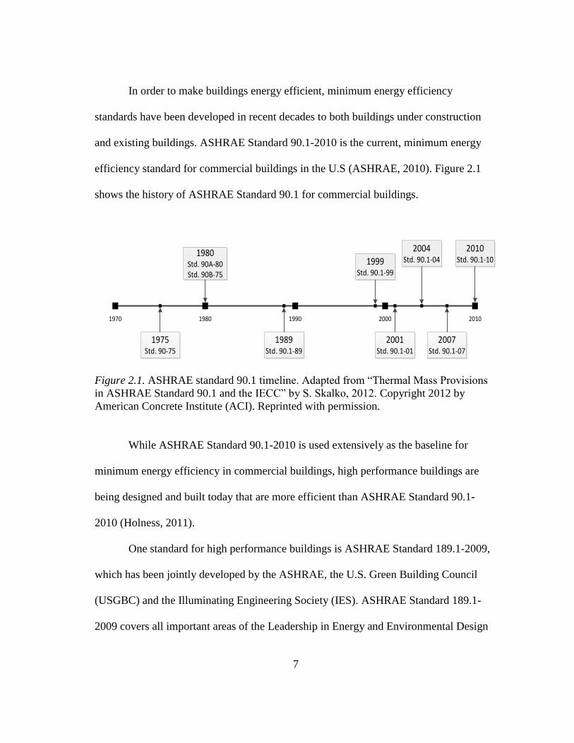
In order to make buildings energy efficient, minimum energy efficiency

standards have been developed in recent decades to both buildings under construction

and existing buildings. ASHRAE Standard 90.1-2010 is the current, minimum energy

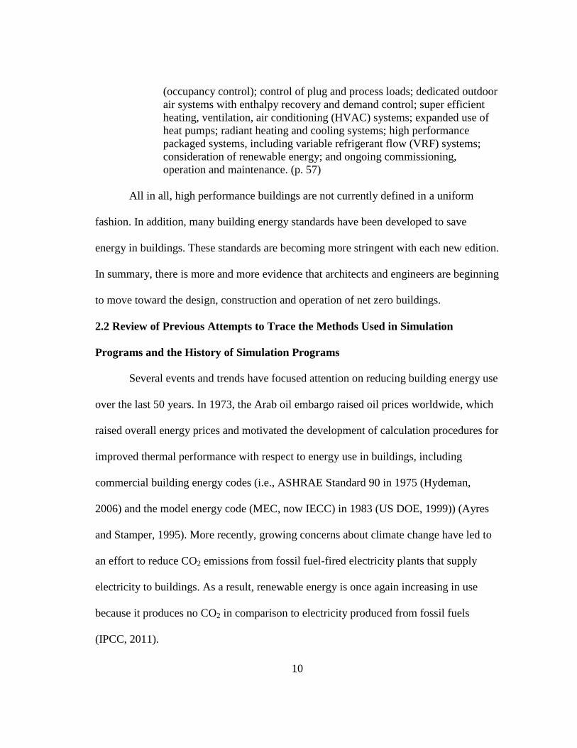
efficiency standard for commercial buildings in the U.S (ASHRAE, 2010). Figure 2.1

shows the history of ASHRAE Standard 90.1 for commercial buildings.

1970

1975Std. 90-75

1980 201020001990

1980Std. 90A-80Std. 90B-75

1989Std. 90.1-89

1999Std. 90.1-99

2001Std. 90.1-01

2004Std. 90.1-04

2007Std. 90.1-07

2010Std. 90.1-10

Figure 2.1. ASHRAE standard 90.1 timeline. Adapted from “Thermal Mass Provisions

in ASHRAE Standard 90.1 and the IECC” by S. Skalko, 2012. Copyright 2012 by

American Concrete Institute (ACI). Reprinted with permission.

While ASHRAE Standard 90.1-2010 is used extensively as the baseline for

minimum energy efficiency in commercial buildings, high performance buildings are

being designed and built today that are more efficient than ASHRAE Standard 90.1-

2010 (Holness, 2011).

One standard for high performance buildings is ASHRAE Standard 189.1-2009,

which has been jointly developed by the ASHRAE, the U.S. Green Building Council

(USGBC) and the Illuminating Engineering Society (IES). ASHRAE Standard 189.1-

2009 covers all important areas of the Leadership in Energy and Environmental Design

8

(LEED) rating system developed by USGBC. This standard is approximately 32% more

efficient than ASHRAE Standard 90.1-2004 (Holness, 2011). In addition, ASHRAE

Standard 189.1-2009 covers “…site sustainability, water use efficiency, energy

efficiency, indoor environmental quality (IEQ), and the building’s impact on the

atmosphere, materials and resources.” (ASHRAE, 2009, p. 4). ASHRAE Standard

189.1-2011, which is the revised version of 189.1-2009, was released in February 2012

(Stanke, 2012). ASHRAE Standard 189.1-2011 provides substantial improvements over

the previous version, including reference to ASHRAE Standard 90.1-2010, which has

more stringent requirements than ASHRAE Standard 90.1-2007 (ASHRAE, 2011;

Stanke, 2012). For example, ASHRAE Standard 90.1-2010 has more stringent

requirements for sidelights and skylights, which ASHRAE Standard 90.1-2007 does not

have. ASHRAE Standard 189.1-2011 also includes a detailed prescriptive option with

respect to a minimum sidelighting effective aperture and a skylight effective aperture,

which ASHRAE Standard 189.1-2009 did not have.

The International Green Construction Code (IGCC), developed by the

International Code Council (ICC), is another standard for high performance commercial

buildings. In addition, the IGCC covers conservation of natural resources, materials,

energy and water. It also has requirements concerning indoor environmental air quality

and owner education. The IGCC can cross-reference ASHRAE Standard 189.1 if a local

jurisdiction adopts it (ICC, 2012).

Net zero energy buildings (NZEBs) are buildings that need energy equal to or

less than the amount of renewable energy provided on-site annually. However, the

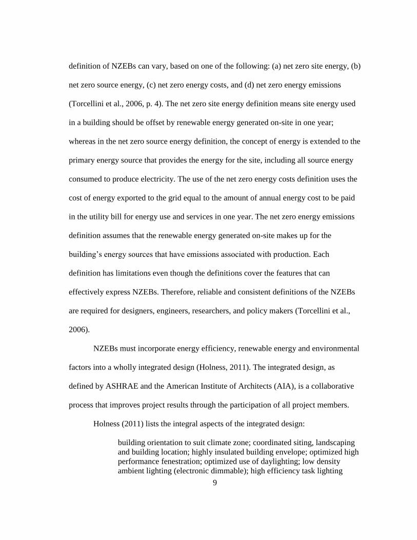
9

definition of NZEBs can vary, based on one of the following: (a) net zero site energy, (b)

net zero source energy, (c) net zero energy costs, and (d) net zero energy emissions

(Torcellini et al., 2006, p. 4). The net zero site energy definition means site energy used

in a building should be offset by renewable energy generated on-site in one year;

whereas in the net zero source energy definition, the concept of energy is extended to the

primary energy source that provides the energy for the site, including all source energy

consumed to produce electricity. The use of the net zero energy costs definition uses the

cost of energy exported to the grid equal to the amount of annual energy cost to be paid

in the utility bill for energy use and services in one year. The net zero energy emissions

definition assumes that the renewable energy generated on-site makes up for the

building’s energy sources that have emissions associated with production. Each

definition has limitations even though the definitions cover the features that can

effectively express NZEBs. Therefore, reliable and consistent definitions of the NZEBs

are required for designers, engineers, researchers, and policy makers (Torcellini et al.,

2006).

NZEBs must incorporate energy efficiency, renewable energy and environmental

factors into a wholly integrated design (Holness, 2011). The integrated design, as

defined by ASHRAE and the American Institute of Architects (AIA), is a collaborative

process that improves project results through the participation of all project members.

Holness (2011) lists the integral aspects of the integrated design:

building orientation to suit climate zone; coordinated siting, landscaping

and building location; highly insulated building envelope; optimized high

performance fenestration; optimized use of daylighting; low density

ambient lighting (electronic dimmable); high efficiency task lighting

10

(occupancy control); control of plug and process loads; dedicated outdoor

air systems with enthalpy recovery and demand control; super efficient

heating, ventilation, air conditioning (HVAC) systems; expanded use of

heat pumps; radiant heating and cooling systems; high performance

packaged systems, including variable refrigerant flow (VRF) systems;

consideration of renewable energy; and ongoing commissioning,

operation and maintenance. (p. 57)

All in all, high performance buildings are not currently defined in a uniform

fashion. In addition, many building energy standards have been developed to save

energy in buildings. These standards are becoming more stringent with each new edition.

In summary, there is more and more evidence that architects and engineers are beginning

to move toward the design, construction and operation of net zero buildings.

2.2 Review of Previous Attempts to Trace the Methods Used in Simulation

Programs and the History of Simulation Programs

Several events and trends have focused attention on reducing building energy use

over the last 50 years. In 1973, the Arab oil embargo raised oil prices worldwide, which

raised overall energy prices and motivated the development of calculation procedures for

improved thermal performance with respect to energy use in buildings, including

commercial building energy codes (i.e., ASHRAE Standard 90 in 1975 (Hydeman,

2006) and the model energy code (MEC, now IECC) in 1983 (US DOE, 1999)) (Ayres

and Stamper, 1995). More recently, growing concerns about climate change have led to

an effort to reduce CO2 emissions from fossil fuel-fired electricity plants that supply

electricity to buildings. As a result, renewable energy is once again increasing in use

because it produces no CO2 in comparison to electricity produced from fossil fuels

(IPCC, 2011).

11

Analysis by hourly computer simulation programs is one way that energy use can

be reduced in buildings at the design stage (ASHRAE TGER, 1975). According to

Kusuda (1999), in 1959, the ASHRAE Journal published the first paper that addressed

how a digital computer could be used to simulate an HVAC system component

(Soumerai et al., 1959). In this study, a Bendix G-15 computer that used assembly

language was used at the Worthington air conditioning company to calculate the cylinder

pressure of a refrigeration compressor. The authors had to work hard for the calculation

because the programming language for the Bendix G-15 was very tedious and limited by

today’s standards. Shortly afterwards in the 1950s, an IBM 7094 computer using

FORTRAN, which was a more powerful programming language, was used for building

simulations at the National Bureau of Standards (NBS). The availability of the IBM

7094 computer using FORTRAN enabled a numerical simulation to be developed that

analyzed the interior thermal environment of fallout shelters in 1964 at NBS even though

the simulation running time was quite long. This simulation achievement using a digital

computer encouraged other engineers including Metin Lokmanhekim, who played an

important role in creating the DOE-2 program at LBNL, to develop the beginnings of

today’s building simulation programs (Kusuda, 1999).

As computers became more powerful, engineers were able to use more detailed

calculation methods, which had previously not been used due to the limited computer

memory for earlier building energy simulations. In addition, with the development of

computers using FORTRAN, which allowed the simulation developers to develop a

program on one computer to be run on another computer, many new programs for

12

simulation were developed that had more flexibility, including programs that allowed the

user to manage varying loads, with different HVAC systems. Eventually, better user

interfaces were also developed (Sowell and Hittle, 1995).

This section discusses the previous studies that traced energy analysis simulation

programs and their analysis methods with respect to whole-building energy use, solar

PV, active solar, passive solar, and lighting and daylighting simulation programs. This

section reviews studies from the 1950s to the present, which roughly follows the

evolution of FORTRAN. The previous studies include: the proceedings of the first

symposium on use of computers for environmental engineering related to buildings held

in 1970 (NBS, 1971); the report funded by the Electric Power Research Institute (EPRI)

for computer programs with solar heating and cooling systems (Feldman and Merriam,

1979); the proceedings of the building energy simulation conference held in 1985 (US

DOE, 1985); the bibliography of available computer programs of HVAC, which is

provided by ASHRAE (Degelman and Andrade, 1986); and ASHRAE 1995 publications

celebrating the 100th

anniversary of ASHRAE (Ayres and Stamper, 1995; Sowell and

Hittle, 1995; Shavit, 1995). Also covered are the previous studies regarding ASHRAE’s

annotated guides (1990, 1996), Kusuda’s IBPSA paper (1999), Haberl and Cho’s paper

(2004), Kota and Haberl’s paper (2009), and a recent report by the Rocky Mountain

Institute (Tupper et al., 2011).

13

2.2.1 Proceedings of the first symposium on use of computers for environmental

engineering related to buildings (Kusuda ed., 1971)

The first symposium with respect to the use of computers for building energy

simulation was held at the National Bureau of Standards (NBS) in Gaithersburg,

Maryland in 1970. This symposium, entitled “Use of Computers for Environmental

Engineering Related to Buildings”, attracted approximately 400 architects, engineers,

and scientists from 12 countries. NBS, ASHRAE, and the Automated Procedures for

Energy Consultants (APEC) sponsored this symposium. The 59 technical papers of this

symposium addressed a wide variety of issues including computer applications for

building heat transfer analysis, loads and energy calculations, HVAC system

simulations, weather data, and computer graphics (Kusuda ed., 1971). Many of the

papers contained detailed listings of the equations and algorithms that were used.

The majority of these proceedings was related to the cooling and heating load

calculations because these were popular topics among building environmental engineers

in the late 1960s (Kusuda ed., 1971). The application of computers to the dynamic

thermal load calculations allowed building engineers to work with more accurate

solutions and methods that better represented a building’s time-varying loads (Tull,

1971; Lokmanhekim, 1971).

In these proceedings, significant historical facts regarding the application of the

computer to building environmental engineering were mentioned several times such as

the ASHRAE algorithms and the Post Office program. However, these proceedings did

not include timeline diagrams that helped readers more easily understand the historical

14

development of building simulation programs and the analysis methods used in the

simulation programs that were discussed.

2.2.2 Building energy analysis computer programs with solar heating and cooling

system capabilities (Feldman and Merriam, 1979)

The 1979 Electric Power Research Institute (EPRI) report by Feldman and

Merriam concluded that several organizations had developed computer analysis

programs for solar heating and cooling systems. The report focused on the available

programs for electric utilities and their customers. Scott Feldman and Richard Merriam

at Arthur D. Little, Inc. investigated 31 computer programs that they selected based on

the criteria outlined in their report. For example, Feldman and Merriam chose programs

that were not merely duplicated from another program; provided detailed information

describing the program; and did not analyze building loads only (i.e., programs that

included a solar system analysis). In general, the characteristics of these programs were

different because they used different analysis methods, system component types and data

requirements. Only a few of the programs reviewed by Feldman and Merriam remain in

use today; many of the programs are no longer in use or have been combined with other

programs. The report is significant because it referenced many studies that contained

detailed information about the computer models and their applications, performance

analyses of solar systems, and the ASHRAE methods used in the computer simulation

models (Feldman and Merriam, 1979). The report also included diagrams and summary

matrices to help readers better understand the capabilities and background of the

simulation programs that were surveyed.

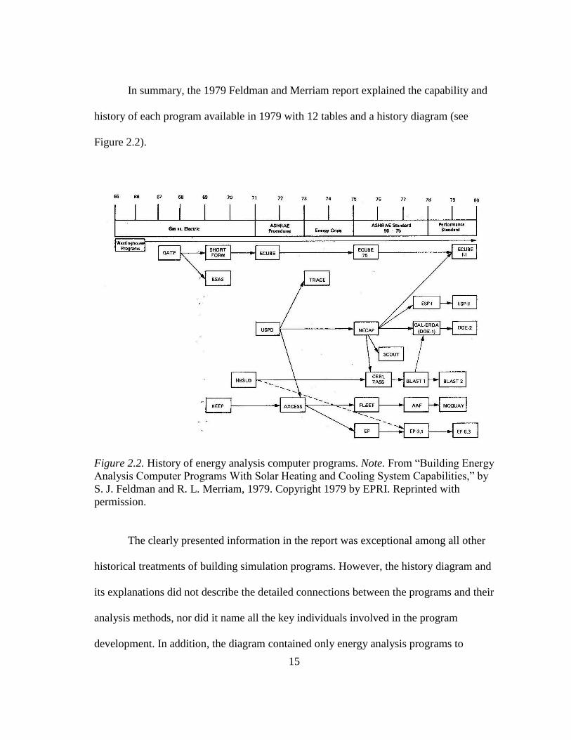
15

In summary, the 1979 Feldman and Merriam report explained the capability and

history of each program available in 1979 with 12 tables and a history diagram (see

Figure 2.2).

Figure 2.2. History of energy analysis computer programs. Note. From “Building Energy

Analysis Computer Programs With Solar Heating and Cooling System Capabilities,” by

S. J. Feldman and R. L. Merriam, 1979. Copyright 1979 by EPRI. Reprinted with

permission.

The clearly presented information in the report was exceptional among all other

historical treatments of building simulation programs. However, the history diagram and

its explanations did not describe the detailed connections between the programs and their

analysis methods, nor did it name all the key individuals involved in the program

development. In addition, the diagram contained only energy analysis programs to

16

compare the background of solar heating and cooling programs. In other words, the

diagram did not show solar heating and cooling programs. Finally, the report was written

in 1979 and only covered computer programs created before then. It was never updated

by EPRI.

2.2.3 Proceedings of the building energy simulation conference (US DOE, 1985)

The Building Energy Simulation Conference held in Seattle, Washington, in

1985 was sponsored by the Passive Solar Group of the United States Department of

Energy (US DOE, 1985). The conference was unique because it was one of the first U.S.

conferences that focused on building energy simulation since the first symposium at

National Bureau of Standards (NBS) in 1970. The proceedings of the conference focused

on effective simulation applications, microcomputer techniques and program

development. Out of a total of 59 papers in the proceedings, 11 papers were about

applications of building energy simulation, 13 papers about the microcomputer

simulation techniques and 22 papers about simulation program development.

The proceedings of the conference also provided an explanation about how

building energy simulation was developed and conducted from the late 1960s until 1985

in a variety of locations, including: North America (Kusuda, 1985), Europe (Sornay and

Clarke, 1985), Asia (Matsuo, 1985) and Oceania (i.e., Australia and New Zealand)

(Mason, 1985). The proceedings also included papers that explained microcomputer

programs such as ECAP (Jansen, 1985) and ESPRE (Merriam, 1985), which contributed

to opportunities for further developing many of today’s energy simulation programs

(Kusuda, 1985). The microcomputer programs referenced in the proceedings used a

17

number of different calculation techniques to calculate energy use in buildings,

including: the Cooling Load Temperature Difference (CLTD) Method (Rudoy and

Duran, 1975); a Resistor-Capacitor (RC) Network Model (Paschkis, 1942); and

Response Factor (Mitalas and Stephenson, 1967) / Weighting Factor (Stephenson and

Mitalas, 1967) Method. Other papers in the proceedings discussed related program

developments for passive solar systems (Gratia 1985; Hayashi et al., 1985; Ishizuka et

al., 1985; Emery et al., 1985). There was also a paper by Winkelmann and Selkowitz

that discussed a daylighting simulation program that was combined into a whole-

building energy simulation program (i.e., DOE-2) (Winkelmann and Selkowitz, 1985).

In summary, the proceedings of this conference covered many of the historical

aspects for building energy simulation and solar simulation programs (i.e., daylighting

and passive solar programs). However, although the proceedings did contain historical

papers, they did not include any papers that contained timeline diagrams to help readers

graphically visualize the sequence and inter-connection of the historical process of

building energy simulation.

2.2.4 A bibliography of available computer programs in the area of heating,

ventilating, air conditioning, and refrigeration (Degelman and Andrade, 1986)

This bibliography described general abstracts and annotated software abstracts of

various simulation programs, including areas of acoustics, computer-aided building

design, mechanical equipment design, energy and economic analysis, heating and

cooling load calculations, lighting, solar systems, psychrometrics, weather data analysis,

and other related areas. This bibliography included information that had been collected

18

until November 1986, which was from domestic and foreign journals, all U.S.

universities, national laboratories, and known software companies. There are two main

sections; Section 1 presents the abstracts categorized by the areas of the simulation

programs, and Section 2 includes cross-reference indices by keyword, computer type,

price category, program name, and author or vendor, which are used for searching the

simulation programs (Degelman and Andrade, 1986).

This bibliography contained the abstracts, operating environment, program

availability and authors of 36 heating and cooling load calculations, 52 energy analysis,

nine solar system analysis, and 18 lighting design and analysis simulation programs. The

abstracts and subsections provided the features, computer types such as microcomputer,

minicomputer, or mainframe computer, source code type, and author of each simulation

program. In addition, some abstracts of these simulation programs explained the analysis

methods used in these simulation programs. However, this bibliography did not explain

the historical development of the analysis methods used in the simulation programs, and

most of the abstracts did not describe which analysis method was used in the simulation

program.

2.2.5 An annotated guide to models and algorithms for energy calculations relating to

HVAC equipment (Yuill, 1990) and annotated guide to load calculation models and

algorithms (Spitler, 1996)

By the 1990s, engineers and researchers had developed many simulation models

that contained thousands of different algorithms to simulate hourly envelope loads and

HVAC system loads for building simulation programs. To help researchers sift through

19

the different programs, ASHRAE sponsored several annotated guides. For example, in

1975, the ASHRAE Task Group on Energy Requirements (TGER) published two books

(ASHRAE, 1975a, 1975b) that included algorithms for load calculation and modeling

methods for HVAC systems and plants in order to computerize building energy analysis.

These ASHRAE annotated guide books were developed because many simulation

program developers spent much of their time searching ASHRAE literature for technical

information to help them write their algorithms. Such demand for this information

directly motivated ASHRAE to develop and publish the annotated guides. The ASHRAE

annotated guides provided explanations and references to help simulation program

developers better understand the algorithms and models used in building computer

programs. The annotated guide book relating to HVAC equipment (Yuill, 1990)

included algorithms relating to the air-handling, refrigeration, heating, unitary and solar

heating equipment, while the annotated guide book for load calculation (Spitler, 1996)

covered building envelope models, entire building loads models and other room heat

transfer models.

In summary, the two ASHRAE annotated guides thoroughly reviewed the

previous references and provided detailed information about the historical development

of the previous algorithms and models for HVAC equipment and load calculations.

However, the guides did not contain detailed timeline diagrams (i.e., family trees or

genealogy charts) that help trace the interconnections of the algorithms and models in

order to better grasp their significance.

20

2.2.6 Historical development of building energy calculations (Ayres and Stamper,

1995)

During the 1970s, companies and government organizations created dozens

peak-load and annual energy use simulation programs. The energy calculation

methodologies used in these simulation programs varied from detailed hourly

simulations to simple steady-state equations. Many of these simulation programs are no

longer in use because of a lack of support, poor documentation, limited technical

upgrades, or discontinuance of the program. A few programs were re-released, updated

and improved over time and included detailed documentation. By 1980, there were

approximately ten major hourly energy analysis programs for large commercial

buildings. However, by 1995, only the proprietary energy simulation programs

developed by Trane, Carrier, the Automated Procedures for Energy Consultants (APEC),

and a few others had survived because their software documentation and support were

satisfactory. Some companies with proprietary software did not want to share the

algorithms of their simulation programs, which often contributed to the demise of the

software. On the other hand, there have been many advances in public domain energy

analysis programs because the shared algorithms made the programs more available to

users, and as a result, received a wider acceptance.

During this period, the government financially supported only a few of the public

programs, which contributed to their success, while at the same time, making it difficult

for private companies to continue to support their programs because of the competition

from the publically-funded programs. In recent years, the U.S. national laboratories,

21

selected educational institutions and a few private companies have focused more on

developing new interfaces for the existing energy simulation programs rather than

developing new calculation methods in order to meet increasing demands for ease-of-use

(Ayres and Stamper, 1995).

Ayres and Stamper used tables and diagrams to help explain the history of the

manual and automated energy calculation methods as well as energy simulation

programs. Their explanations included information about the basic analysis methods, the

historical background of why simulation programs became important, and which

organizations developed or supported the simulation programs. The paper concluded that

many proprietary energy analysis programs had difficulty surviving, while only a few

public domain building energy simulation programs survived beyond 1995.

In summary, the Ayres and Stamper paper showed that today’s energy analysis

programs for buildings were developed from only a few peak-load and annual energy

calculation computer programs. The paper also contained a useful family tree type

diagram for the public domain programs (see Figure 2.3).

22

Figure 2.3. Family trees of public domain programs. Note. From “Historical

Development of Building Energy Calculations,” by J. M. Ayres and E. Stamper, 1995,

ASHRAE Transactions, 37, p.847. Copyright 1995 by ASHRAE2 (www.ashrae.org).

Reprinted with permission.

However, there were few explanations about the diagram and no details that

explained the connections between the public domain programs and the earlier energy

analysis programs in terms of the analysis methods used to analyze building energy use,

or the authors of the earlier analysis methods.

2.2.7 Evolution of building energy simulation methodology (Sowell and Hittle, 1995)

According to the paper by Sowell and Hittle (1995), the generally available

public domain energy analysis programs for buildings use one of two methods to

2 ASHRAE address: 1791 Tullie Circle, N.E. Altlanta, GA 30329

23

calculate the heating and cooling loads in buildings. One method, called the weighting

factor method (Mitalas and Stephenson, 1967), calculates cooling or heating loads with

pre-calculated weighting factors or custom weighting factors. Weighting factors are used

to convert heat gains through walls or roofs to heating or cooling loads in a zone. The

other method is the heat balance method that uses a conductive, convective, and

radiative heat balance for all room surfaces in the thermal zone. These two methods for

calculating a building’s hourly heating and cooling loads have been applied in most

major public domain programs. Each method has advantages and limitations, which

affect the performance of the energy programs. For example, the weighting factor

method does not require repeated calculations for simulation, and the heat balance

method does not need the assumptions of constant convection conditions (Sowell and

Hittle, 1995).

Sowell and Hittle explained the development of the load, system, plant, and

economics (LSPE) simulation sub-programs. They also compared the two main public

domain programs that existed prior to 1995 (i.e., DOE-2 and BLAST) that used the two

methods (i.e., the weighting factor method for DOE-2 and the heat balance method for

BLAST). However, the paper did not have a historical diagram or complete explanations

of all the references in the development process of the LSPE algorithms in the two

methods. Finally, since the paper was written in 1995, it did not cover analysis methods

written since then that are contained in today’s public domain programs (i.e,

EnergyPlus).

24

2.2.8 Short-time-step analysis and simulation of homes and buildings during the last

100 years (Shavit, 1995)

Short-time-step analysis and hourly simulation programs for buildings have been

under development for the last 100 years, which has included three time periods: pre-

World War II, from World War II (1945) to the second energy crisis (1973), and a

period representing the post-second energy crisis. In contrast to the hourly energy

simulation programs, the short-time-step analysis programs were designed to evaluate

building heating and cooling loads on a minute-by-minute basis for use when simulating

the performance of a building’s HVAC controls simulation. Such an analysis using a

short-time-step was able to simulate short-time-steps for thermal systems in almost real

time. However, hourly whole-building programs were used to analyze an entire

building’s annual energy use because of the long computing time required by the short-

time-step programs (Shavit, 1995).

Shavit explained the pre-1960s historical aspects of the analysis methods that

contributed to the development of building simulation programs. Shavit’s paper made an

important contribution because it is difficult to find detailed explanations about any pre-

1960s analysis methods in other papers. Before digital computers were used for building

analysis in the 1960s, engineers used analog computers, which used an electric circuit

analogy (i.e., actual resistors and capacitors), to simulate the time-dependent thermal

behavior (Willcox et al., 1954; Buchberg, 1955; Buchberg 1958). The electric circuit

25

analogy greatly influenced the thermal analysis calculations in all succeeding simulation

programs, including short-time-step and whole-building simulation programs.

Shavit’s paper also provided comparisons between the short-time-step programs

and whole-building simulation programs. Finally, this paper provided useful information

about short-time-step programs and their uses in control simulations. In addition, the

paper provided a timeline diagram that included both short-time-step programs and

hourly whole-building simulation programs from 1967 to 1986 (see Figure 2.4). Like the

diagram of the 1979 EPRI report, Shavit’s diagram included the lineage of several

additional privately developed programs (i.e., TRACE and ECUBE). However, the

diagram did not explain from where the analysis methods in these programs originated.

Unfortunately, Shavit did not provide sufficient explanations and references necessary

for a complete understanding of the history diagram in the paper.

26

Figure 2.4. Development timeline of simulation programs. Note. From “Short-Time-Step Analysis and Simulation of Homes

and Buildings During the Last 100 Years,” by G. Shavit, 1995, ASHRAE Transactions, 101, p. 864. Copyright 1995 by

ASHRAE (www.ashrae.org). Reprinted with permission.

27

2.2.9 Early history and future prospects of buildings system simulation (Kusuda, 1999)

According to Kusuda (1999), in the early 1960s, the U.S. government developed

the first computerized thermal simulations to analyze fallout shelters to determine what

interior conditions would be like in the heavy underground concrete structures. Around

this same time, gas and electric companies such as the Westinghouse Electric Company

and a group of gas industry companies, called Gas Application to Total Energy

(GATE), also started producing general-purpose thermal simulations for buildings based

on hourly calculations. This trend motivated ASHRAE to form the Task Group on

Energy Requirements (TGER) in 1967 to develop a public-domain, whole-building

energy simulation program with hourly load calculations. Also, in 1967, the Automated

Procedure for Engineering Consultants (APEC) developed a loads calculation program

(HCC) that used the Total Equivalent Temperature Differential (TETD)/Time Averaging

(TA) method, which was better-suited to run on the small computers that had limited

memory, which were used by HVAC engineers at that time (Kusuda, 1999).

In his paper, Kusuda also discussed his experience with the detailed development

of thermal simulation analysis methods, including specific analysis methods for

psychometric calculations, room air motion using Computational Fluid Dynamics (CFD)

and heating and cooling load calculations. In each of these discussions, Kusuda also

discussed the historical aspects of each method and provided references to organizations

or individuals that contributed to the development of the analysis methods. Kusuda also

provided his view of future prospects for building simulation programs based on his

more than 30 years of experience and knowledge writing simulation programs.

28

In summary, Kusuda’s paper covered his personal simulation experience from

the 1950s to the 1970s including the detailed development of analysis methods and their

historical significance. The information in this paper was also based in part on his

experience, which is important because he contributed significantly to the development

of many of the original analysis methods that are still used in simulation programs today.

However, his paper did not have a historical diagram to help the reader visually

understand the hierarchy and genealogy of the analysis methods he discussed. Also, even

though the paper was published in 1999, Kusuda did not include the most recent state-of-

the-art programs (i.e., EnergyPlus) and their analysis methods in his discussion.

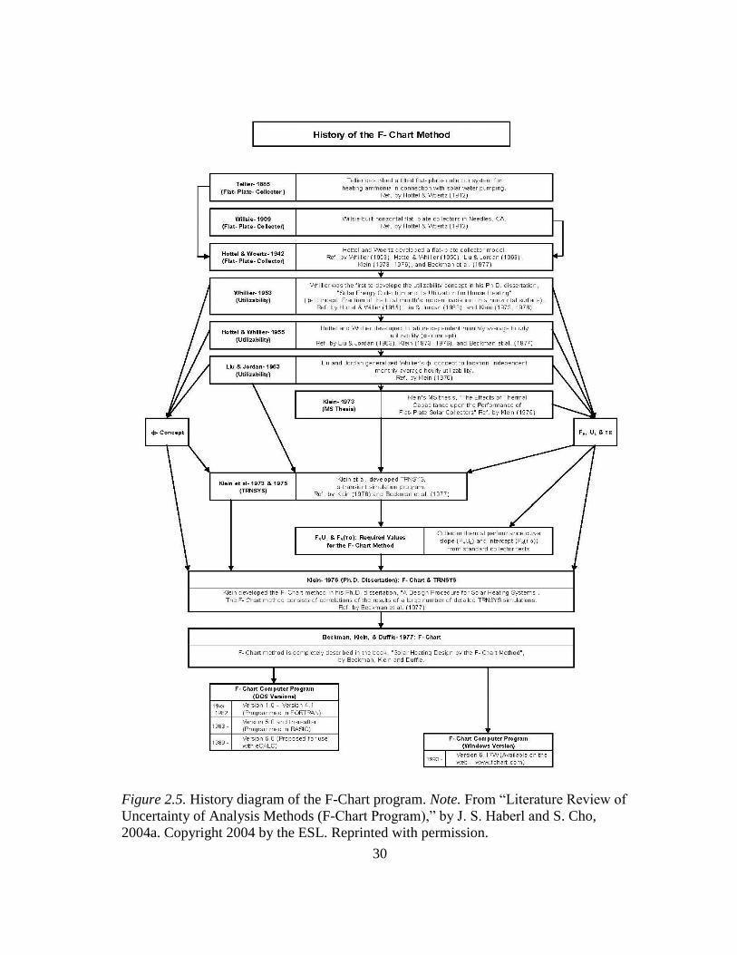
2.2.10 Literature review of uncertainty of analysis methods (F-Chart, PV F-Chart ,

and DOE-2 program) (Haberl and Cho, 2004a, 2004b, 2004c)

Haberl and Cho wrote three reports in 2004. Haberl and Cho’s first report in

2004 traced the lineage of the F-Chart method, which originated from Sanford Klein’s

Ph.D. dissertation (Klein, 1976). The F-Chart program uses the F-Chart method, also

developed by Klein, which estimates the fraction F of heating loads generated from solar

energy (Klein, 1993). Correlations using data from many TRNSYS simulation runs,

which analyzed specific solar heating systems, were used to create the F-Chart equations

(Klein et al., 1976). The F-Chart program can be used to design solar heating systems by

deciding what size and type of solar collectors are best for a given heating load and the

domestic hot water (DHW) system of a building (Haberl and Cho, 2004a). The second

report traced the roots of the PV F-Chart program that can be used to analyze

photovoltaic systems, utility interface, and battery storage systems. Klein and Beckman

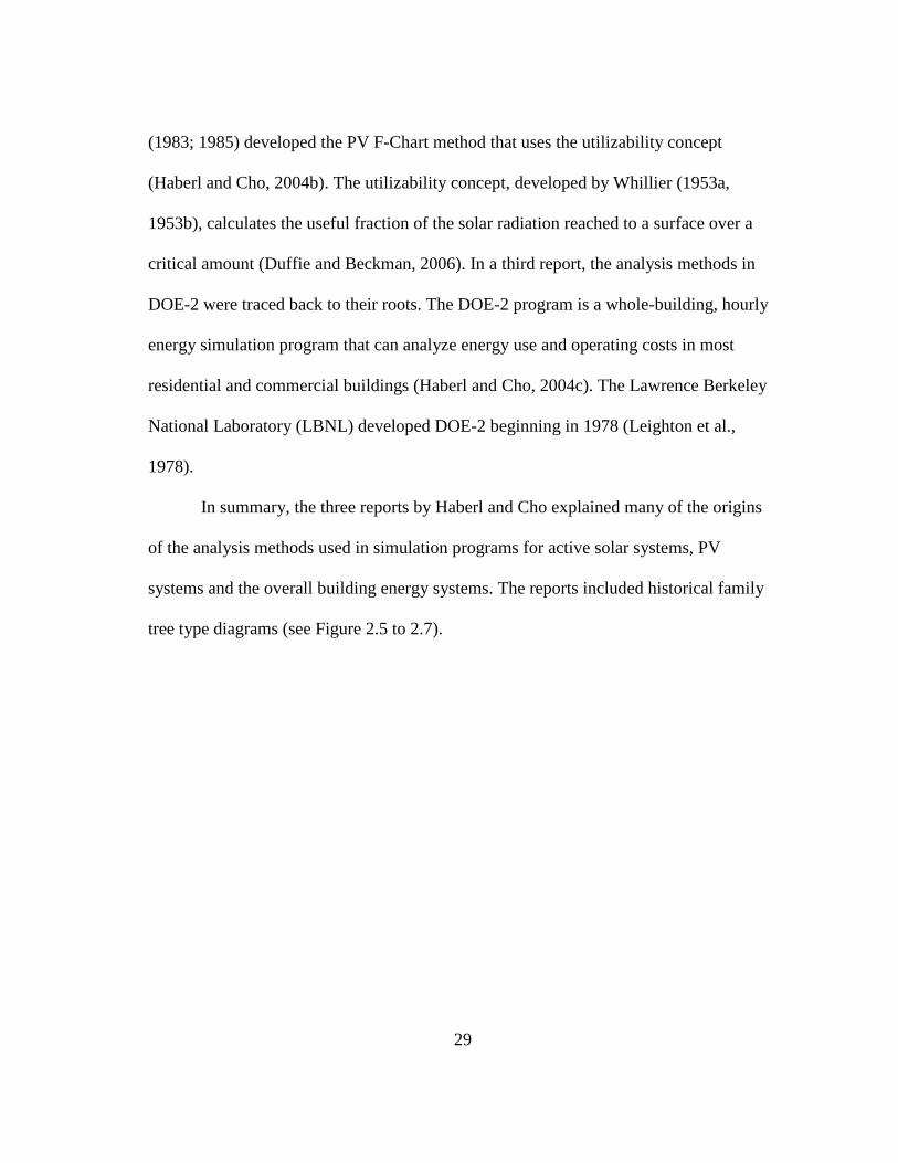
29

(1983; 1985) developed the PV F-Chart method that uses the utilizability concept

(Haberl and Cho, 2004b). The utilizability concept, developed by Whillier (1953a,

1953b), calculates the useful fraction of the solar radiation reached to a surface over a

critical amount (Duffie and Beckman, 2006). In a third report, the analysis methods in

DOE-2 were traced back to their roots. The DOE-2 program is a whole-building, hourly

energy simulation program that can analyze energy use and operating costs in most

residential and commercial buildings (Haberl and Cho, 2004c). The Lawrence Berkeley

National Laboratory (LBNL) developed DOE-2 beginning in 1978 (Leighton et al.,

1978).

In summary, the three reports by Haberl and Cho explained many of the origins

of the analysis methods used in simulation programs for active solar systems, PV

systems and the overall building energy systems. The reports included historical family

tree type diagrams (see Figure 2.5 to 2.7).

30

Figure 2.5. History diagram of the F-Chart program. Note. From “Literature Review of

Uncertainty of Analysis Methods (F-Chart Program),” by J. S. Haberl and S. Cho,

2004a. Copyright 2004 by the ESL. Reprinted with permission.

31

Figure 2.6. History diagram of the PV F-Chart program. Note. From “Literature Review

of Uncertainty of Analysis Methods (PV F-Chart Program),” by J. S. Haberl and S. Cho,

2004b. Copyright 2004 by the ESL. Reprinted with permission.

32

Figure 2.7. History diagram of the DOE-2 simulation program. Note. From “Literature

Review of Uncertainty of Analysis Methods (DOE-2 Program),” by J. S. Haberl and S.

Cho, 2004c. Copyright 2004 by the ESL. Reprinted with permission.

33

These three historical diagrams provided detailed information about the analysis

methods in a straightforward and clear diagram that used a branching, family tree

format. However, each report only treated the analysis methods of the specific program

(i.e., F-Chart, PV F-Chart and DOE-2 program) and did not provide any linkage between

the programs. In other words, the first report covered only the F-Chart program, the

second report only the PV F-Chart program and the third report only the DOE-2

program. In addition, the three reports did not cover other programs in use today (i.e.,

EnergyPlus), nor have they been updated since they were published.

2.2.11 Contrasting the capabilities of building energy performance simulation

programs (Crawley et al., 2005)

Various whole-building simulation programs have been developed to use in

saving energy in buildings since the 1970s. In 2005, Crawley et al.’s paper reviewed the

features of 20 whole-building simulation programs including: BLAST (Hittle, 1977),

BSim , DeST (Chen and Jiang, 1999), DOE-2.1e (Winkelmann et al., 1993), ECOTECT

(Marsh, 1996), Ener-Win (Degelman, 1990), Energy Express (Moller, 1996), Energy-10,

EnergyPlus (Crawley et al., 2001), eQUEST (LBNL and JJH, 1998), ESP-r (Energy

Systems Research Unit, 2002; Clarke, 1982, 2001), IDA ICE (Sahlin et al, 2003), IES

<VE>, HAP (Carrier, 2003), HEED (Milne, 2004), PowerDomus (Mendes et al., 2003),

SUNREL (Deru et al, 2002), Tas, TRACE (Trane, 1992), and TRNSYS (Klein et al.,

1976). In the paper, overviews of 20 simulation programs were described and 14 tables

were presented to compare the specific areas of 20 programs including: general

modeling features; zone loads; building envelope and daylighting; infiltration,

34

ventilation and multizone airflow; renewable energy systems; electrical systems and

equipment; HVAC systems; HVAC equipment; economic evaluation; climate data

availability; results reporting; validation; user interface, links to other programs, and

availability (Crawley et al., 2005).

Among the many comparative papers and surveys for building simulation

programs, this paper provided the most comprehensive comparisons for specific features

using 14 tables and their footnotes. However, the tables utilized information provided by

vendors, which may not have had an adequate peer-review (Crawley et al., 2005). In

addition, even though the overviews and tables of 20 simulation programs describe

analysis methods used in the programs, they did not explain where the analysis methods

originated, and who or which organization contributed to the development of the

analysis methods.

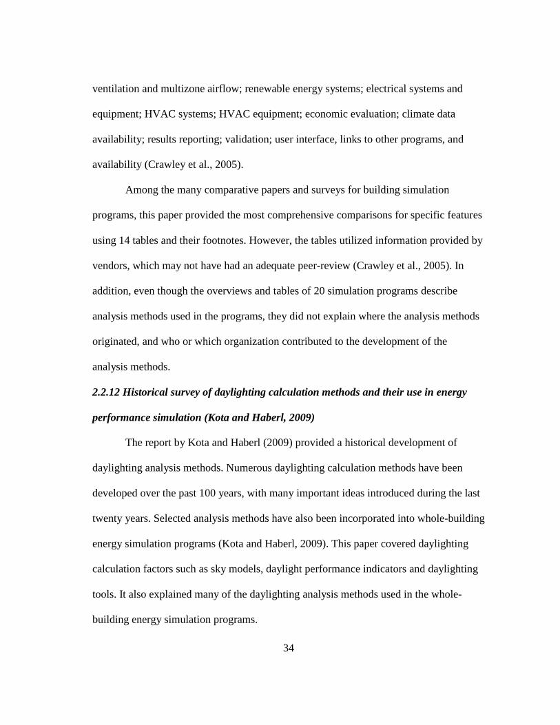
2.2.12 Historical survey of daylighting calculation methods and their use in energy

performance simulation (Kota and Haberl, 2009)

The report by Kota and Haberl (2009) provided a historical development of

daylighting analysis methods. Numerous daylighting calculation methods have been

developed over the past 100 years, with many important ideas introduced during the last

twenty years. Selected analysis methods have also been incorporated into whole-building

energy simulation programs (Kota and Haberl, 2009). This paper covered daylighting

calculation factors such as sky models, daylight performance indicators and daylighting

tools. It also explained many of the daylighting analysis methods used in the whole-

building energy simulation programs.

35

In summary, this paper traced the origins of the methods used in the daylighting

simulation programs and the development process of the daylighting calculations

methods. This paper also included a detailed historical family tree diagram (see Figure

2.8). Although the historical diagram seemed to be the only known analysis that

provided such detailed information, it was presented in a somewhat confusing diagram

with several parallel paths, different line types crossing back and forth between paths

and, unfortunately, used a very small font that made the diagram difficult to read.

Finally, the report has also not been updated since it was published.

2.2.13 Pre-read for Building Energy Modeling (BEM) innovation summit (Tupper et

al., 2011)

RMI, ASHRAE, IBPSA, USGBC, and the Institute for Market Transformation

(IMT) recognized the need for collaboration among stakeholders in the field of building

energy modeling. In the spring of 2011, RMI hosted the first BEM Innovation Summit

with other organizations in Boulder, Colorado to work together to develop widespread

use of BEM solutions for analysis of high performance buildings. This report was

published with the purpose of explaining the history and present situation of the BEM

industry in the U.S to all participants of the BEM innovation summit (Tupper et al.,

2011).

36

Figure 2.8. History diagram of the daylighting calculation methods and the daylighting

simulation programs. Note. From “Historical Survey of Daylighting Calculations

Methods and Their Use in Energy Performance Simulations,” by S. Kota and J. S.

Haberl, 2009. Copyright 2009 by the ESL. Reprinted with permission.

37

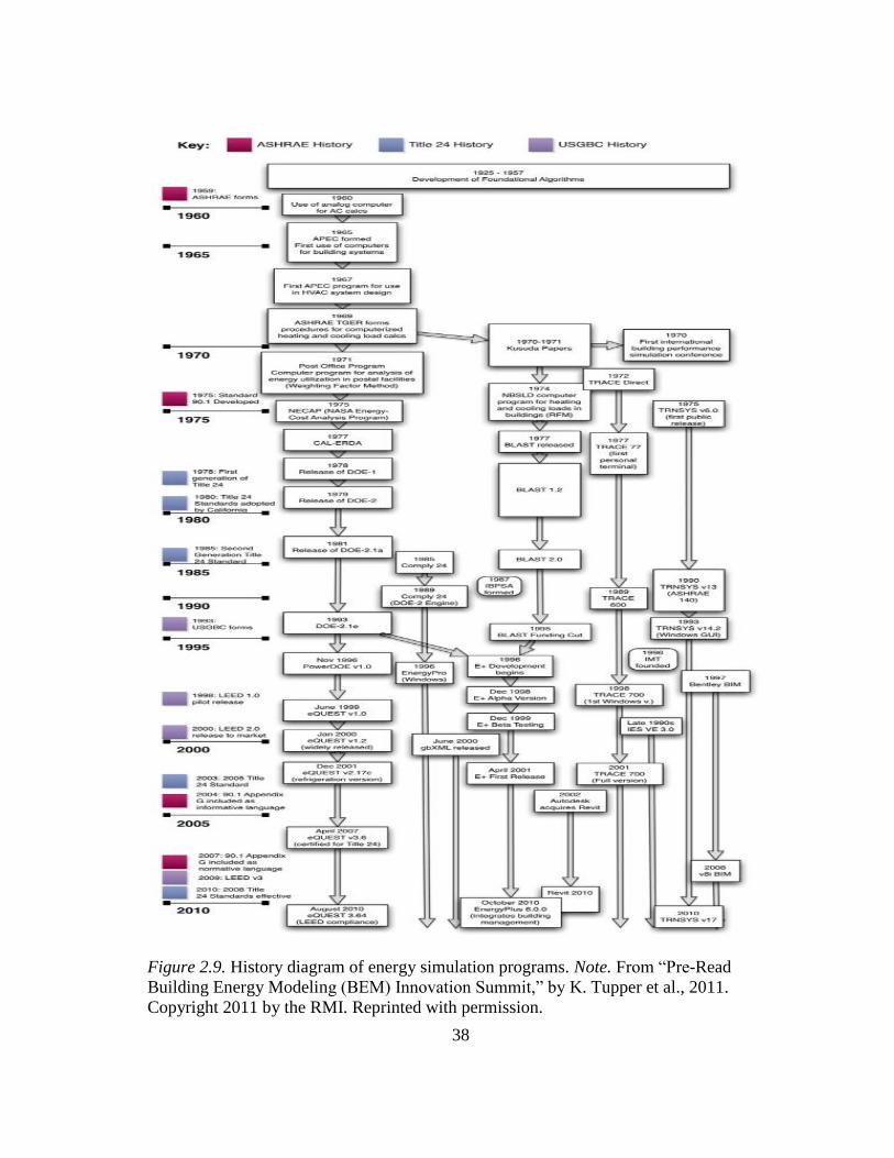
In this pre-read report, there was a section that discussed the history of BEM.

This section provided a historical explanation and a historical flow chart that graphically

displayed the evolution of BEM. The flow chart highlighted the development of many

different building energy software programs including their release date and also

indicated key organizations that contributed to the simulation development along the

timeline. Much of the flow chart and accompanying explanation was adapted from

Haberl and Cho’s (2004c) third report with additional information provided by personal

communications with selected building simulation experts.

In summary, the history section of the RMI report explained the history of

selected analysis methods, simulation programs, and organizations from the pre-1960s to

the present using a timeline diagram (see Figure 2.9). However, it did not discuss the

different analysis methods in each simulation program, and the boxes in the flow chart

contained inconsistent content. For example, some boxes had explanations of building

simulation programs and funding organizations, whereas other boxes only marked the

names of the simulation programs and organizations. In addition, the boxes of the flow

chart were cluttered and not as well organized as other historical diagrams. Finally, the

flowchart was based on Haberl and Cho’s diagram (see Figure 4), which did not trace all

the programs in the RMI report. The RMI report also did not have all the references for

the flow chart. Therefore, a more detailed diagram or flow chart with additional

information still needs to be developed.

38

Figure 2.9. History diagram of energy simulation programs. Note. From “Pre-Read

Building Energy Modeling (BEM) Innovation Summit,” by K. Tupper et al., 2011.

Copyright 2011 by the RMI. Reprinted with permission.

39

2.3 Summary of Literature Review

This literature review included a review of the different definitions of high

performance buildings using the most widely used standards, a review of the history of

the methodologies and simulations used to analyze high performance buildings with

respect to the development of computer technology, and a review of the previous studies

that investigated the methods used in simulation programs and traced the history of

simulation programs. The previous studies reviewed included: historical traces of whole-

building energy simulation; solar PV, active solar and passive solar system simulation;

and lighting and daylighting simulation programs. Table 2.1 shows the areas covered by

the previous studies. Table 2.2 shows which previous literature had historical diagrams

and the features of the historical diagrams that were reviewed. Each of areas of the

previous studies is summarized as follows:

Whole-Building Energy Simulation: Several of the previous studies covered the

history of whole-building energy simulations and their analysis methods.

Fifteen studies discussed the history of whole-building energy simulations among

the sixteen studies that were reviewed. Five history diagrams were provided

among the fifteen studies. These history diagrams varied in format and included

timelines and family tree-type diagrams to help readers better understand the

relationship and development of the analysis methods in the simulation

programs. However, some history diagrams had no connections between

simulation programs and their analysis methods, while others had connection but

presented little about what analysis methods were shared. Many have not been

40

updated since the studies were written, some of which are now 17 years old.

Other history diagrams did not have detailed information about the relevant

individual boxes in the history diagrams. One of most insightful discussions had

no diagram to accompany the discussions (i.e., Kusuda’s paper in 1999).

Solar System Simulation: Four literature (i.e., EPRI report in 1979, Proceedings

of the building energy simulation conference in 1985, and Haberl and Cho’s

reports in 2004) covered the history of solar system simulations. Two literature

contained history diagrams of the solar system simulations (i.e., Haberl and

Cho’s reports in 2004). The history diagrams showed detailed information

including brief explanations and references. However, the diagrams did not

compare many solar simulation programs and their analysis methods. Also, the

diagrams did not include information about organizations supporting the

development of the solar system simulation programs.

Lighting & Daylighting Simulation: Only one of the previous papers included a

history diagram of lighting and daylighting simulation programs (i.e., Kota and

Haberl’s report in 2009). This historical diagram presented brief explanations and

references from 1895 to 2006. However, the diagram was constructed with

somewhat confusing parallel paths with several line types crossing back and forth

between the paths and, unfortunately, used a very small font that was difficult to

read.

41

Table 2.1. Catalog of previous studies that identified the analysis methods used in simulation programs for high performance

commercial buildings.

Paper Title Author /

Year

Whole-Building Energy Solar Systems Lighting &

Daylighting Load

Calculation

HVAC

Systems PV System

Active Solar

System

Passive Solar

System

Proceedings of the

first symposium on

use of computers for

environmental

engineering related to

buildings

Kusuda, T.

(Ed.) /

1971

● ●

Building Energy

Analysis Computer

Programs with Solar

Heating and Cooling

System Capabilities

Feldman &

Merriam /

1979

● ● ● ● ●

Building Energy

Simulation

Conference

Notebook

US DOE /

1985 ● ● ●

A bibliography of

available computer

programs in the area

of heating,

ventilating, air

conditioning, and

refrigeration

Degelman

& Andrade

/

1986

● ● ● ● ● ●

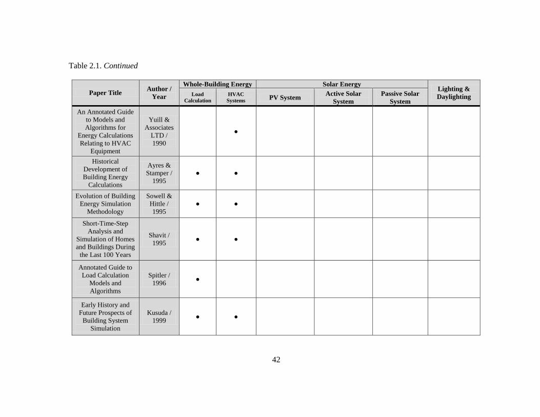
42

Table 2.1. Continued

Paper Title Author /

Year

Whole-Building Energy Solar Energy Lighting &

Daylighting Load

Calculation

HVAC

Systems PV System

Active Solar

System

Passive Solar

System

An Annotated Guide

to Models and

Algorithms for

Energy Calculations

Relating to HVAC

Equipment

Yuill &

Associates

LTD /

1990

●

Historical

Development of

Building Energy

Calculations

Ayres &

Stamper /

1995

● ●

Evolution of Building

Energy Simulation

Methodology

Sowell &

Hittle /

1995

● ●

Short-Time-Step

Analysis and

Simulation of Homes

and Buildings During

the Last 100 Years

Shavit /

1995 ● ●

Annotated Guide to

Load Calculation

Models and

Algorithms

Spitler /

1996 ●

Early History and

Future Prospects of

Building System

Simulation

Kusuda /

1999 ● ●

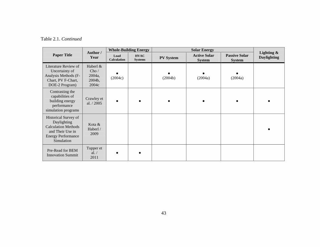
43

Table 2.1. Continued

Paper Title Author /

Year

Whole-Building Energy Solar Energy Lighting &

Daylighting Load

Calculation

HVAC

Systems PV System

Active Solar

System

Passive Solar

System

Literature Review of

Uncertainty of

Analysis Methods (F-

Chart, PV F-Chart,

DOE-2 Program)

Haberl &

Cho /

2004a,

2004b,

2004c

●

(2004c)

●

(2004b)

●

(2004a)

●

(2004a)

Contrasting the

capabilities of

building energy

performance

simulation programs

Crawley et

al. / 2005 ● ● ● ● ● ●

Historical Survey of

Daylighting

Calculation Methods

and Their Use in

Energy Performance

Simulation

Kota &

Haberl /

2009

●

Pre-Read for BEM

Innovation Summit

Tupper et

al. /

2011

● ●

44

Table 2.2. Coverage of the previous literature including features of the diagram found in the previous studies.

Paper Title Author /

Year

Literature

Covered

Year

Literature

Topic

History

Diagram

Existence

History Topic

History Diagram Features

Advantages Disadvantages

Proceedings of the first symposium

on use of

computers for environmental

engineering

related to buildings

Kusuda,

T. (Ed.) /

1971

Pre-1971

Whole-

Building

Simulation

No

Whole-

Building

Simulation

Mentioned significant historical facts

regarding the application of the

computer to building environmental engineering several times such as the

ASHRAE algorithms and the Post

Office program.

Did not include timeline diagrams

that helped readers more easily

understand the historical development of building simulation

programs and the analysis methods

used in those simulation programs.

Building Energy

Analysis Computer

Programs with

Solar Heating and Cooling System

Capabilities

Feldman

& Merriam /

1979

1960s - 1970s

Whole-

Building

Simulation

Yes

Whole-

Building

Simulation

Displayed various whole-building simulation programs.

Did not explain the connections

between the programs and their algorithms. Not updated after 1980.

Not explained in detail.

Building Energy Simulation

Conference

Notebook

US DOE /

1985

1960s -

1985

Whole-

Building Simulation /

Solar

Systems Simulation

No

Whole-

Building Simulation

Covered many of the historical aspects for building energy simulation and solar

simulation programs (i.e., daylighting

and passive solar programs).

Did not include any papers that

contained timeline diagrams to help readers graphically visualize the

sequence and inter-connection of the

historical process of building energy simulation.

A bibliography of available computer

programs in the

area of heating, ventilating, air

conditioning, and

refrigeration

Degelma &

Andrade /

1986

Pre-1987

Whole- Building /

Solar

Systems / Lighting &

Daylighting

Simulations

No No

Contained the abstracts, operating

environment, program availability and

authors of 36 heating and cooling load calculations, 52 energy analysis, nine

solar system analysis, and 18 lighting

design and analysis simulation programs. The abstracts and

subsections provided the features,

computer types such as microcomputer,

minicomputer, or mainframe computer,

source code type, and author.

Did not explain the historical development of the analysis methods

used in the simulation programs, and

most of the abstracts did not describe which analysis method was used in

the simulation program.

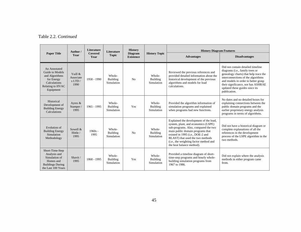
45

Table 2.2. Continued

Paper Title Author /

Year

Literature

Covered

Year

Literature

Topic

History

Diagram

Existence

History Topic History Diagram Features

Advantages Disadvantages

An Annotated Guide to Models

and Algorithms

for Energy Calculations

Relating to HVAC

Equipment

Yuill &

Associate

s LTD /

1990

1958 - 1990

Whole-

Building Simulation

No

Whole-

Building Simulation

Reviewed the previous references and

provided detailed information about the

historical development of the previous algorithms and models for load

calculations.

Did not contain detailed timeline

diagrams (i.e., family trees or

genealogy charts) that help trace the

interconnections of the algorithms

and models in order to better grasp

their significance, nor has ASHRAE updated these guides since its

publication.

Historical

Development of Building Energy

Calculations

Ayres &

Stamper /

1995

1965 - 1995

Whole-

Building

Simulation

Yes

Whole-

Building

Simulation

Provided the algorithm information of

simulation programs and explained

when programs had new functions.

No dates and no detailed boxes for explaining connections between the

public domain programs and the

earlier proprietary energy analysis programs in terms of algorithms.

Evolution of

Building Energy

Simulation Methodology

Sowell & Hittle /

1995

1960s -

1995

Whole- Building

Simulation

No Whole-

Building

Simulation

Explained the development of the load,

system, plant, and economics (LSPE)

sub-programs. Also, compared the two

main public domain programs that

existed in 1995 (i.e., DOE-2 and BLAST) that used the two methods

(i.e., the weighting factor method and

the heat balance method).

Did not have a historical diagram or

complete explanations of all the references in the development

process of the LSPE algorithm in the

two methods.

Short-Time-Step

Analysis and Simulation of

Homes and

Buildings During the Last 100 Years

Shavit /

1995 1868 - 1995

Whole-

Building Simulation

Yes

Whole-

Building Simulation

Provided a timeline diagram of short-time-step programs and hourly whole-

building simulation programs from

1967 to 1986.

Did not explain where the analysis

methods in either program came from.

46

Table 2.2. Continued

Paper Title Author /

Year

Literature

Covered

Year

Literature

Topic

History

Diagram

Existence

History Topic History Diagram Features

Advantages Disadvantages

Annotated Guide

to Load

Calculation

Models and Algorithms

Spiter / 1996

1958 - 1996

Whole-

Building

Simulation

No

Whole-

Building

Simulation

Reviewed the previous references and

provided detailed information about the

historical development of the previous

algorithms and models for HVAC equipment.

Did not contain detailed timeline diagrams (i.e., family trees or

genealogy charts) that help trace the

interconnections of the algorithms and models in order to better grasp

their significance, nor has ASHRAE

updated these guides since its publication.

Early History and

Future Prospects of Building

System Simulation

Kusuda / 1999

1950s - 1970s

Whole-

Building

Simulation

No

Whole-

Building

Simulation

Covered Kusuda’s personal simulation

experience from the 1950s to 1970s

including the detailed development of analysis methods and their historical

significance. The information in this

paper was also based in part on his experience, which is significantly

important because he contributed

significantly to the development of many of the original analysis methods

that are still used in simulation

programs today.

Did not have a historical diagram to

help the reader visually understand

the hierarchy and genealogy of the analysis methods he discussed. Also,

even though the paper was published

in 1999, Kusuda did not include the most recent state-of-the-art programs

(i.e., EnergyPlus) and their analysis

methods in his discussion.

Literature Review

of Uncertainty of Analysis Methods

(F-Chart Program)

Haberl &

Cho /

2004a

1885 - 1993

Solar

Thermal

Systems

Yes Solar Thermal

Systems Provided detailed information and straightforward diagram paths.

Did not compare other similar

programs and their analysis methods. The diagram covered only the F-

Chart program.

Literature Review

of Uncertainty of Analysis Methods

(PV F-Chart

Program)

Haberl & Cho /

2004b

1953 - 1993 Solar PV

Systems Yes

Solar PV

Systems Same as above.

Did not compare other similar

programs and their analysis methods.

The diagram covered only the PV F-Chart program.

47

Table 2.2. Continued

Paper Title Author /

Year

Literature

Covered

Year

Literature

Topic

History

Diagram

Existence

History Topic History Diagram Features

Advantages Disadvantages

Literature Review of Uncertainty of

Analysis Methods

(DOE-2 Program)

Haberl &

Cho /

2004c

1925 - 2003

Whole-

Building

Simulation

Yes

Whole-

Building

Simulation

Same as above.

Did not compare other similar programs and their analysis methods.

The diagram covered only the DOE-

2 program.

Contrasting the

capabilities of

building energy performance

simulation

programs

Crawley

et al. /

2005

Pre-2006

Whole-

Building / Solar

Systems /

Lighting & Daylighting

Simulations

No No

Provided the comparisons in the most specific areas using 14 tables and their

footnotes among many comparative

papers and surveys for building simulation programs.

Utilized information provided by vendors, which may not have had an

adequate review (Crawley et al.,

2005). Did not explain where the analysis methods originated, and

who or which organization

contributed to the development of the analysis methods.

Historical Survey

of Daylighting

Calculation

Methods and Their

Use in Energy Performance

Simulation

Kota &

Haberl /

2009

1895 - 2007 Lighting & Daylighting

Yes Lighting & Daylighting

Provided detailed information including references and explanations.

Presented in a somewhat confusing

diagram flow with several line types

and footnotes, as well as a small font

that was difficult to read in the diagram.

Pre-Read for BEM Innovation

Summit

Tupper et

al. / 2011 1925 - 2011

Whole- Building

Simulation

Yes Whole-

Building

Simulation

Explained several simulation programs and organizations from pre 1960s to

present.

Did not compare the analysis

methods of each simulation program.

Also, the boxes of the diagram contained inconsistent content. The

boxes of the diagram were cluttered.

Finally, this diagram was based on Haberl and Cho’s partially

developed diagram; therefore, more

detailed information should be

added.

48

In summary, although there have been many attempts at tracing the history of

analysis methods used in whole-building, solar, and lighting and daylighting simulation

programs, all of the previous attempts have some limitations. Therefore, there is a need

for a more comprehensive and improved history diagram, which includes origins and

brief explanations of the important analysis methods in the simulation programs for

whole-building, solar PV, active solar, passive solar, lighting and daylighting simulation

programs. Such comprehensive analysis is needed because if simulation users knew

more about the analysis methods in the simulation programs and their origins, some of

the current problems and obstacles in applying the building simulation program might be

resolved (Tupper et al., 2011). For example, today, different building simulation users do

not achieve the same modeling results, even when they use the same programs to

simulate the same building, using the same weather data. Also, in general, simulation

users who did not create the simulation program usually do not completely comprehend

what the simulation program can simulate without an extensive review of all the

program analysis methods, defaults and calculation logic (RMI, 2011).

49

CHAPTER III

METHODOLOGY

3.1 Overview of Methodology

The methodology of this study is provided in this chapter. The objectives of this

study are as follows: (a) to review and analyze the previous literature in order to trace

the origins of the analysis methods contained in widely-used simulation programs in the

U.S.; (b) to develop a consistent, comprehensive historical diagram that resolves

discrepancies in the previous diagrams; (c) to identify the key roles of individuals and

organizations that have contributed significantly to the development of simulation

programs; and (d) to identify the important analysis methods of the most widely used

programs, where the analysis methods came from, who developed the methods, and how

the programs use the capabilities of the analysis methods to simulate high performance

buildings. With these objectives, the following tasks were performed:

1. Identify the major groups of simulation programs that are used to analyze high

performance buildings in the U.S. Review each group of simulation programs and trace

the origins of the simulation programs to the original source of the key analysis methods.

2. Develop a new comprehensive history diagram (i.e., genealogy chart).

2.1. Identify the analysis methods used in the simulation programs.

2.2. Accurately analyze the historical facts of the previous studies.

2.3. Add relevant historical information about the analysis methods to identify

from where the analysis methods originated.

50

3. Review the new comprehensive genealogy chart with key experts of each program

group.

4. Complete and analyze the new genealogy chart by time period, by specific

organization or funding, by specific analysis method, and by specific simulation

program.

In order to better describe the origins of analysis methods used in today’s

simulation programs, a new comprehensive history diagram was created. Figure 3.1

shows the steps involved with this methodology. The following sections explain the

details of each procedure. 15 simulation programs which are divided into three groups

are studied in this research (Section 3.2). The overall features of each program are

briefly described in the summary table of Section 3.2.4. A description about how each

group of simulation programs was reviewed is explained in Section 3.2. The procedures

used to create the new comprehensive history diagram are presented in Section 3.4.

Finally, an analysis of the history diagram using four approaches (i.e., time period,

specific analysis methods, specific simulation programs, and specific organizations or

funding) is presented in Section 3.5.

51

Identification of Major Groups of Simulation Programs

Review of Each Group of the Simulation Programs by Tracing the Origins of the Analysis Methods Used in

the Simulation Programs

Development of a New Comprehensive History Diagram (Genealogy Chart)

Analysis of the Genealogy Chart

By time periodBy tracing specific analysis methods

By tracing specific simulation programs

By tracing the influence of specific

organizations, funding, etc.

Identify the analysis methods used in the simulation programs

Accurately analyze the historical facts of the

previous studies

Add relevant historical information about the

analysis methods to identify from where the analysis

methods originated

Identification and Data Collection

Development of

a New Genealogy Chart

Analysis of

the New Genealogy Chart

Presentation of the Genealogy Chart

Review of the Genealogy Chart by Key Experts of Each Program Group

Review of the Genealogy Chart

Figure 3.1. Procedures for developing and discussing the new comprehensive genealogy

chart.

3.2 Identification of Major Groups of Simulation Programs

There are numerous simulation programs for analyzing high performance

buildings (EERE, 2013a). These simulation programs can be categorized by three groups

(i.e., whole-building analysis, solar energy analysis, and lighting and daylighting

52

analysis) that are seen in Figure 3.2. These three groups were chosen primarily because

of the different organizations that supported them. Some of the simulation programs

appear in more than one group.

Radiance

eQUEST/DOE-2.2

DOE-2.1eEnergyPlus TRNSYSTRACE HAP

F-Chart/TRNSYS

PV F-Chart/TRNSYS

SLR Method/PASOLE

Lighting & Daylighting Analysis Simulation

EnergyPlus Daylighting

Whole-Building Energy Simulation

SUNREL/SERIRES

DAYSIM DOE-2.1e Daylighting

Solar Thermal Design

Lumen-Micro

Solar PV Design

Passive Solar Simulation

Solar Energy Analysis Simulation

Figure 3.2. Three groups of simulation programs by different organizations.

The major U.S. organization that has contributed significantly to the

development of whole-building energy simulation programs is the American Society of

Heating, Refrigerating and Air Conditioning Engineers (ASHRAE). In addition to

53

ASHRAE, several national institutes such as the National Institute of Standards and

Technology or NIST (formerly the National Bureau of Standards or NBS) and the U.S.

Postal Service (USPS), national laboratories – the Lawrence Berkeley National

Laboratory or LBNL (foremerly the Lawrence Berkeley Laboratory or LBL), Argonne

National Laboratory (ANL), and Los Alamos National Laboratory or LANL (formerly

Los Alamos Scientific Laboratory or LASL) contributed to the development of the

whole-building energy simulation programs. Several consulatants and academic

institutes also contributed the development. These include the Computational

Consultants Bureau (CCB), GARD Analytics (formerly known as the General American

Research Division (GARD) of the General American Transportation Corporation

(GATX)), the University of Illinois at Urbana-Champaign (UIUC), and Oklahoma State

University (OSU). The first symposium at the NBS in 1970 successfully continues to the

present time as the IBPSA conference. Most of the financial support of the whole-

building simulation development has come from the U. S. Department of Energy (US

DOE).

The major U.S. contributors to the development of solar energy analysis

programs include: the American Society of Mechanical Engineers (ASME) Solar Energy

Division (SED) and the American Solar Energy Society (ASES) of the International

Solar Energy Society (ISES). The US DOE financially supported the simulation

development of solar energy systems since 1972. Several national laboratories and

universities conducted studies for simulation development under the sponsorship of the

US DOE. The national laboratories include LASL (now, LANL), the Solar Energy

54

Research Institute (SERI) (now, the National Renewable Energy Laboratory or NREL),

and the Sandia National Laboratory (SNL). The universities include the University of

Wisconsin-Madison (UWM) and Colorado State University (CSU).

The major U.S. contributor to the development of lighting and daylighting

analysis programs is the Illuminating Engineering Society of North America (IESNA).

The LBL (now LBNL) has been the major developer for lighting and daylighting

simulations in the U.S. since 1976 when there was strong national interest for employing

daylighting strategies into new energy efficient building design.

These three different groups appear to have worked separately due to their

different stated objectives even though the end result contributed to integrated high

performance building simulations. Therefore, the simulation programs in this study were

classified by the three different groups. Six whole-building analysis simulation

programs, four solar energy analysis programs, and five lighting and daylighting

simulation programs were studied, and the results presented on the new chart.

3.2.1 Whole-building energy simulation programs

In general, hourly whole-building analysis programs calculate all the hourly

energy that is consumed or generated by an entire building over the period of one year.

These whole-building simulation programs take into account the effects of weather,

internal loads and occupants’ energy-use patterns to calculate how different HVAC

systems meet the heating and cooling loads. In this study, EnergyPlus (Crawley et al.,

2001), DOE-2.1e (Winkelmann et al., 1993), eQUEST/DOE2.2 (Hirsch, 1998), TRACE

55

(Trane, 1992), HAP (Carrier, 2003), and TRNSYS (Klein et al., 1976) were studied as

whole-building analysis simulation programs.

3.2.2 Solar energy simulation programs

Solar energy can be used to heat air or water using various solar systems, or it

can be used to generate electricity. In this study, the following types of solar energy

design or simulation programs were studied: solar thermal, solar PV, and passive solar.

3.2.2.1 Solar thermal design program

Solar thermal simulation programs are used to analyze solar thermal systems

such as active solar thermal systems (i.e., solar collectors and thermal storage units) and

solar domestic hot water (SDHW) systems. In this study, one solar thermal design

program, which is called the F-Chart program (Klein and Beckman, 2001a), was traced

and analyzed. This program uses the F-Chart method, which was created by correlations

of many simulation runs using TRNSYS, a simulation program (Klein et al., 1976).

3.2.2.2 Solar Photovoltaic (PV) design program

Solar PV, also called solar cells, converts sunlight (i.e., solar radiation) directly

into electricity. The PV F-Chart program (Klein and Beckman, 2001b), which is based

on the F-Chart method and Clark et al.’s method (Clark et al., 1984), can be used to

evaluate the long-term performance of PV systems. This program was traced and

analyzed as the solar PV design program in this study.

3.2.2.3 Passive solar simulation program

Passive solar houses use solar heating directly (i.e., without pumps, blowers, etc.)

and sometimes include natural passive cooling. For example, solar direct gain,

56

sunspaces, Trombe walls, and passive down-draft cooltowers3 are passive solar

strategies. SUNREL (Deru et al., 2002) currently can be used to calculate the

effectiveness of different types of passive solar buildings. SUNREL based on SERIRES

uses the solar geometry equations by McFarland in 1979 and the solar declination

equation by Duffie and Beckman in 1991 (Deru et al., 2002). PASOLE, which was

introduced in 1978, analyzes passive solar buildings. A correlation using results from

over hundred simulation runs through PASOLE (i.e., the detailed simulation program)

created the Solar Load Ratio (SLR) method, which is a method for estimating the

required solar collector array size for space heating without active solar systems

(Balcomb, 1992). In this study, these programs were traced and analyzed as passive solar

simulation programs. In addition, the F-Chart program, previously classified as a solar

thermal simulation program, can also be used to analyze selected passive solar systems,

such as passive direct gain and a passive storage wall.

3.2.3 Lighting and daylighting simulation program

Daylighting strategies use natural light to reduce the electricity loads of artificial

electric lighting systems. A proper daylighting design can provide improved illumination

for occupants and can reduce a building’s energy use. Building orientation, window size,

and shading (i.e., overhangs and fins) are used to calculate the lighting levels at specific

points in a space. Such programs can also keep track of how much artificial lighting is

3 The passive down-draft cooltower uses the evaporation of water to cool the incoming air at the top of a

tower (i.e., chimney). The incoming air, cooled by the evaporation effect, becomes heavier and falls down

through the tower and cools inside of a building. This passive design has been applied to the visitor center

of Zion National Park, designed by NREL (Torcellini, 2000).

57

needed to supplement the daylighting illumination to meet predetermined lighting levels.

The simulation programs for lighting and daylighting analysis used in this study are

DAYSIM (Reinhart and Herkel, 2000; Reinhart and Walkenhorst, 2001), Radiance

(Ward, 1994), the daylighting model in EnergyPlus (i.e., DElight) (Crawley et al, 2001),

the daylighting routines in DOE-2.1e (Winkelmann and Selkowitz, 1985), and the

daylighting routines in Lumen Micro (DiLaura, 1982)4.

3.2.4 Scope and summary table of each simulation program

In this study, the simulation programs in each group were selected based upon

the following criteria: (a) the simulation program is widely used in the U.S., (b) the

program and its documentation are publically available in English throughout the U.S.,

(c) the simulation program or a derivative of the program is still presently in use and

supported, and (d) the analysis method used in the simulation program has made a large

contribution toward the development of simulation (i.e., building thermal, solar thermal,

solar PV, passive solar, or daylighting).

The features of each simulation program are summarized in Table 3.1. The

authors and sponsoring agencies are also included in the table. The abstract column

contains the capabilities and other features. The historical significance column provides

a discussion of why the simulation program is important regarding the development of

simulation programs of each area. This column also presents how a simulation program

affects other simulation programs.

4 Information about the development of the lighting and daylighting simulation programs was reviewed

based on Kota’s doctoral proposal in 2011.

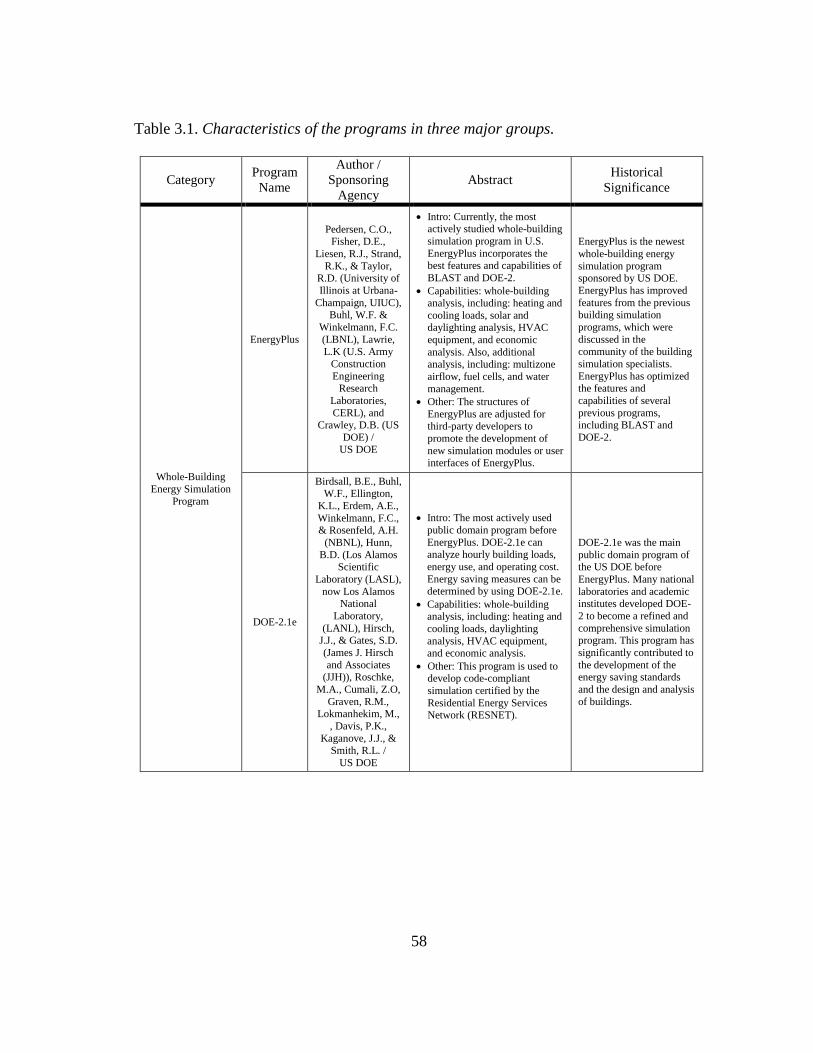
58

Table 3.1. Characteristics of the programs in three major groups.

Category Program

Name

Author /

Sponsoring

Agency

Abstract Historical

Significance

Whole-Building

Energy Simulation

Program

EnergyPlus

Pedersen, C.O., Fisher, D.E.,

Liesen, R.J., Strand,

R.K., & Taylor, R.D. (University of

Illinois at Urbana-

Champaign, UIUC), Buhl, W.F. &

Winkelmann, F.C.

(LBNL), Lawrie,

L.K (U.S. Army

Construction

Engineering Research

Laboratories,

CERL), and Crawley, D.B. (US

DOE) / US DOE

Intro: Currently, the most actively studied whole-building

simulation program in U.S.

EnergyPlus incorporates the best features and capabilities of

BLAST and DOE-2.

Capabilities: whole-building analysis, including: heating and

cooling loads, solar and daylighting analysis, HVAC

equipment, and economic

analysis. Also, additional analysis, including: multizone

airflow, fuel cells, and water

management.

Other: The structures of

EnergyPlus are adjusted for third-party developers to

promote the development of

new simulation modules or user interfaces of EnergyPlus.

EnergyPlus is the newest

whole-building energy

simulation program sponsored by US DOE.

EnergyPlus has improved

features from the previous building simulation

programs, which were

discussed in the

community of the building

simulation specialists.

EnergyPlus has optimized the features and

capabilities of several

previous programs, including BLAST and

DOE-2.

DOE-2.1e

Birdsall, B.E., Buhl, W.F., Ellington,

K.L., Erdem, A.E.,

Winkelmann, F.C., & Rosenfeld, A.H.

(NBNL), Hunn,

B.D. (Los Alamos Scientific

Laboratory (LASL),

now Los Alamos National

Laboratory,

(LANL), Hirsch, J.J., & Gates, S.D.

(James J. Hirsch

and Associates (JJH)), Roschke,

M.A., Cumali, Z.O,

Graven, R.M., Lokmanhekim, M.,

, Davis, P.K.,

Kaganove, J.J., & Smith, R.L. /

US DOE

Intro: The most actively used

public domain program before

EnergyPlus. DOE-2.1e can analyze hourly building loads,

energy use, and operating cost.

Energy saving measures can be determined by using DOE-2.1e.

Capabilities: whole-building analysis, including: heating and

cooling loads, daylighting

analysis, HVAC equipment, and economic analysis.

Other: This program is used to develop code-compliant

simulation certified by the

Residential Energy Services Network (RESNET).

DOE-2.1e was the main

public domain program of the US DOE before

EnergyPlus. Many national

laboratories and academic institutes developed DOE-

2 to become a refined and

comprehensive simulation program. This program has

significantly contributed to

the development of the energy saving standards

and the design and analysis

of buildings.

59

Table 3.1. Continued

Category Program

Name

Author /

Sponsoring

Agency

Abstract Historical

Significance

Whole-Building

Energy Simulation

Program

eQUEST/

DOE-2.2

eQuest: James J.

Hirsch and Associates (JJH) /

non-Government funding

DOE-2.2:

Simulation

Research Group at

LBNL & James J. Hirsch and

Associates (JJH) /

US DOE, the Electric Power

Research Institute

(EPRI), & JJH

Intro: The most widely used whole-building simulation

program that has a user-

friendly graphical user interface including a building creation

wizard, 3D building geometry

display, a graphical HVAC layout, and graphical

simulation results.

Capabilities: whole-building analysis, including: heating and

cooling loads, solar and

daylighting analysis, HVAC equipment, and economic

analysis.

Other: The simulation engine

of eQUEST is DOE 2.2

developed from the DOE 2.1e version 087, which was

released in 1995. This DOE 2.2

engine analyzes window, lighting, and HVAC systems

more accurately and flexibly

than the DOE 2.1e version 087.

eQUEST is the proprietary

version of DOE-2.1e, owned by JJH, developed

in 1999. eQUEST is only

an existing version of

DOE-2 series. This

program uses DOE 2.2

developed from the DOE 2.1e version 087, which

was released in 1995. DOE

2.1e has not been worked on since 2003.

TRNSYS

Klein, S. A.,

Beckman, W. A., & Duffie, S. A. (Solar

Energy Laboratory,

Univ. of Wisconsin-Madison) /

US DOE

Intro: Flexible, modular simulation program that has a

library of models of system

components written as FORTRAN subroutines. A

module includes algebraic or

differential equations that can be modified by users.

Capabilities: whole-building analysis, including HVAC

analysis and sizing, multizone

airflow, electric power simulation, solar design,

building thermal performance,

and analysis of control schemes.

Other: TRNSYS was used to develop the F-Chart method

and PV F-Chart method.

TRNSYS is a widely used

modular or component-

based program since 1975. This program has made a

major contribution to

building energy simulation programs, solar thermal

simulations, and PV

analysis.

TRACE Trane Company

Intro: Load and energy calculation program by the

Trane company.

Capabilities: TRACE can

evaluate several alternatives to

save building energy, including: building envelopes,

HVAC systems and equipment,

and economic combinations.

Other: TRACE provides the

choice of eight cooling load methods and the algorithms

developed by ASHRAE.

A proprietary program for

load and energy

calculations since 1980.

60

Table 3.1. Continued

Category Progra

m Name

Author /

Sponsoring

Agency

Abstract Historical

Significance

Whole-Building

Energy Simulation

Program

HAP Carrier Company

Intro: Hourly analysis program by the Carrier company.

Capabilities: HAP can calculate building loads and system

sizes.

Other: HAP uses ASHRAE’s

Transfer Function Method

(TFM) for thermal loads and the System-Based Design

concept, which is based on

ASHRAE’s Heat Extraction

Method, for system sizes.

Graphical user interface is

used.

A proprietary program for

load and energy

calculations since 1980.

Solar

Energy

Analysis

Simulation

or Design

Program

Solar

Thermal

Analysis

F-

CHART / TRNSYS

Klein, S. A. &

Beckman, W. A. (Solar Energy

Laboratory, Univ.

of Wisconsin-

Madison)

Intro: Comprehensive solar

system analysis and design program.

Capabilities: The system

options contain: water and building storage heating,

domestic hot water, integral

collector-storage DHW, passive direct-gain, passive collector-

storage wall, pebble bed

storage heating, indoor and outdoor pool heating. The

collector options include flat-

plates, evacuated types, compound parabolic

concentrating (CPC) collectors,

and 1or 2 axis tracking types. F-CHART also provides

thermal performance and

economic analysis.

Other: F-Chart uses utilizability

methods to analyze active solar heating systems and un-

utilizability method to estimate

passive direct-gain systems and storage wall systems.

Proven long-term analysis

program for active and passive solar systems. The

analysis method of this

program originated from

Whillier in1953.

Solar

PV

Analysis

PV F-

CHART / TRNSYS

Klein, S. A. &

Beckman, W. A.

(Solar Energy Laboratory, Univ.

of Wisconsin-Madison)

Intro: Comprehensive photovoltaic

(PV) system analysis and design

program.

Capabilities: PV F-CHART

analyzes: monthly estimates of

utility interface systems, battery

storage systems, and stand-alone

systems. The tracking options

include fixed, 1or 2 axis tracking,

and concentrators. Also, it provides

economic analysis.

Other: PV F-CHART uses

utilizability methods to estimate the

weather variation effect regarding

the long-term average performance

of PV systems.

Proved long-term analysis program for PV systems.

The analysis method of this program originated

from Whillier in1953.

61

Table 3.1. Continued

Category Progra

m Name

Author /

Sponsoring

Agency

Abstract Historical

Significance

Solar

Energy

Analysis

Simulation

or Design

Program

Passive

Solar

Analysis

Solar Load

Ratio

(SLR) Method /

PASOLE

PASOLE:

McFarland, R. D.

(LASL (now LANL))

SLR Method: Balcomb, J. D., &

McFarland, R. D.

(LASL (now LANL))

Intro: A research program that incorporates a thermal network

solution by specifying nodes that represent finite regions.

Capabilities: PASOLE analyzes passive solar heated structures

and contains models and

algorithms for calculating solar sources in a general framework.

Provides simulation support for

a design method related to

passive solar heating.

Other: SLR method uses a

simplified monthly calculation procedure depending on

correlations that are the ratio of

solar gain to building load. The correlations are results from

thousands of hourly simulations

developed at LASL (i.e., PASOLE).

SLR method is a widely-

used method to calculate

passive solar buildings since 1978. PASOLE was

used to provide the

correlation parameters of the SLR method.

SUNREL

National Renewable

Energy Laboratory (NREL)

Intro: The whole-building simulation program, most

suitable for passive solar

buildings.

Capabilities: SUNREL contains

modeling of moveable

insulation, interior shading control, Trombe walls, water

walls, advanced glazings,

schedulable window shading, active-charge/passive-discharge

thermal storage, phase change

materials, and natural ventilation.

Other: SUNREL is used for the building physics and

mathematics engine in Targeted

Retrofit Energy Analysis Tool (TREAT), developed for single

and multifamily building

analysis software.

SUNREL is the upgraded

version of SERIRES developed by SERI (now

NREL) in 1983. Currently

used program for passive solar strategies.

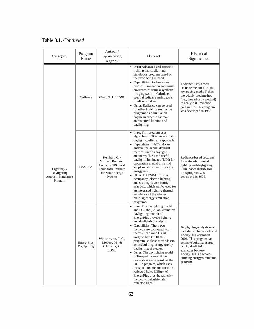
62

Table 3.1. Continued

Category Program

Name

Author /

Sponsoring

Agency

Abstract Historical

Significance

Lighting &

Daylighting Analysis Simulation

Program

Radiance Ward, G. J. / LBNL

Intro: Advanced and accurate lighting and daylighting

simulation program based on the ray-tracing method.

Capabilities: Radiance can predict illumination and visual

environment using a synthetic

imaging system. Calculates spectral radiance and spectral

irradiance values.

Other: Radiance can be used

for other building simulation

programs as a simulation

engine in order to estimate architectural lighting and

daylighting.

Radiance uses a more

accurate method (i.e., the ray-tracing method) than

the widely used method

(i.e., the radiosity method) to analyze illumination

parameters. This program

was developed in 1988.

DAYSIM

Reinhart, C. /

National Research Council (NRC) and

Fraunhofer Institute

for Solar Energy Systems

Intro: This program uses algorithms of Radiance and the

daylight coefficients approach.

Capabilities: DAYSIM can

analyze the annual daylight

metrics: such as daylight autonomy (DA) and useful

daylight illuminance (UDI) for

calculating annual glare and supplemental electric lighting

energy use.

Other: DAYSIM provides

occupancy, electric lighting,

and shading device hourly schedule, which can be used for

an integrated lighting-thermal

simulation of the whole-building energy simulation

programs.

Radiance-based program

for estimating annual lighting and daylighting

illuminance distribution.

This program was developed in 1998.

EnergyPlus

Daylighting

Winkelmann, F. C., Modest, M., &

Selkowitz, S /

LBNL

Intro: The daylighting model and DElight (i.e., an alternative

daylighting model) of

EnergyPlus provide lighting and daylighting analysis.

Capabilities: These two methods are combined with

thermal loads and HVAC

analysis like the DOE-2 program, so these methods can

assess building energy use by

daylighting strategies.

Other: The daylighting model

of EnergyPlus uses three calculation steps based on the

DOE-2 program, which uses

the split-flux method for inter-reflected light. DElight of

EnergyPlus uses the radiosity

method to calculate inter-reflected light.

Daylighting analysis was included in the first official

EnergyPlus version in

2001. This program can estimate building energy

use by daylighting

strategies because

EnergyPlus is a whole-

building energy simulation

program.

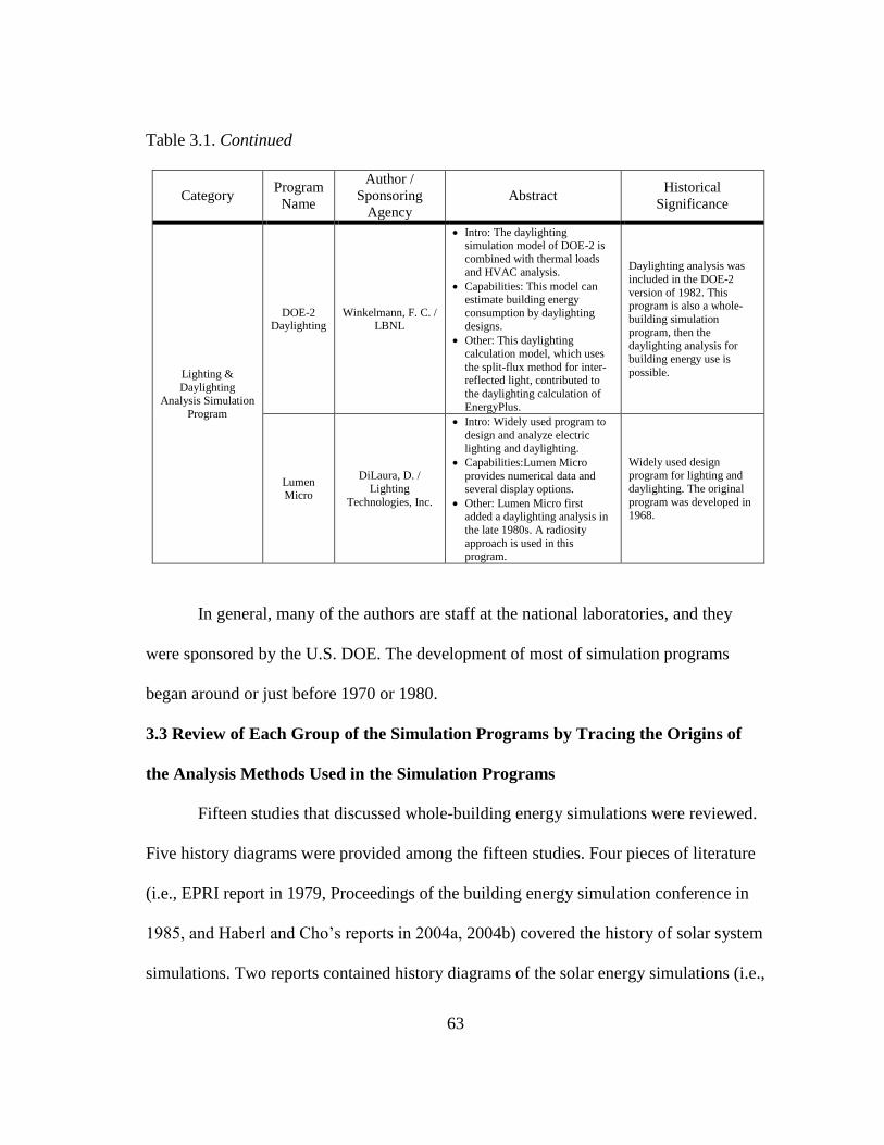
63

Table 3.1. Continued

Category Program

Name

Author /

Sponsoring

Agency

Abstract Historical

Significance

Lighting &

Daylighting Analysis Simulation

Program

DOE-2 Daylighting

Winkelmann, F. C. / LBNL

Intro: The daylighting simulation model of DOE-2 is

combined with thermal loads and HVAC analysis.

Capabilities: This model can estimate building energy

consumption by daylighting

designs.

Other: This daylighting

calculation model, which uses

the split-flux method for inter-

reflected light, contributed to

the daylighting calculation of

EnergyPlus.

Daylighting analysis was

included in the DOE-2

version of 1982. This program is also a whole-

building simulation

program, then the daylighting analysis for

building energy use is

possible.

Lumen Micro

DiLaura, D. /

Lighting

Technologies, Inc.

Intro: Widely used program to

design and analyze electric lighting and daylighting.

Capabilities:Lumen Micro

provides numerical data and several display options.

Other: Lumen Micro first added a daylighting analysis in

the late 1980s. A radiosity

approach is used in this program.

Widely used design program for lighting and

daylighting. The original

program was developed in 1968.

In general, many of the authors are staff at the national laboratories, and they

were sponsored by the U.S. DOE. The development of most of simulation programs

began around or just before 1970 or 1980.

3.3 Review of Each Group of the Simulation Programs by Tracing the Origins of

the Analysis Methods Used in the Simulation Programs

Fifteen studies that discussed whole-building energy simulations were reviewed.

Five history diagrams were provided among the fifteen studies. Four pieces of literature

(i.e., EPRI report in 1979, Proceedings of the building energy simulation conference in

1985, and Haberl and Cho’s reports in 2004a, 2004b) covered the history of solar system

simulations. Two reports contained history diagrams of the solar energy simulations (i.e.,

64

Haberl and Cho’s reports in 2004a, 2004b). Only one of the previous papers included a

history diagram of lighting and daylighting simulation programs (i.e., Kota and Haberl’s

report in 2009).

Unfortunately, the previous studies and diagrams did not provide the connections

between the analysis methods and the simulation programs. Therefore, there is a need for

a more comprehensive and improved history diagram, which includes origins and brief

explanations of the important analysis methods in the simulation programs for whole-

building, solar PV, active solar, passive solar, lighting and daylighting simulation

programs. In addition, none of diagrams have been updated since the studies were

written. The limitations could be resolved by analyzing the original references cited in

all the previous studies as well as the new published studies.

3.4 Development of a New Comprehensive History Diagram

After analyzing the original references cited in all the previous studies, a new

comprehensive history diagram was created. This new diagram included the three

different groups of simulation programs and included key analysis methods and their

authors as well as institutions. In order to display all the information in this new

diagram, the diagram was oriented horizontally, running across several pages. In this

new diagram, special attention has been paid to connect the analysis methods to the

simulation programs that codified the original analysis methods.

3.4.1 Identify the analysis methods used in the simulation programs

Several analysis methods are used in today’s whole-building energy, solar

energy, and lighting and daylighting simulation programs. Table 3.2 indicates which

65

analysis methods were traced in this study. The primary types of analysis methods can

be categorized by the type of building parameters. Therefore, this table was designed to

aid in describing the new comprehensive history diagram. In this study, a selection of the

primary analysis methods was chosen for analyzing the origins of the simulation

programs.

Table 3.2. Analysis methods of the simulation programs.

Group Selected

Parameter Analysis Method Program Name

Whole-Building

Energy Simulation

Program

Zone Thermal

Loads

Heat Balance Method EnergyPlus

Weighting Factor Method DOE-2.1e

Weighting Factor Method eQUEST/DOE-2.2

Finite-Difference and

Network Approach / Heat

Balance Method

TRNSYS

Weighting Factor Method,

Cooling Load Temperature

Difference / Cooling Load

Factor Method, Total Equivalent

Temperature Differential / Time

Averaging Method, or Radiant

Time Series Method

TRACE

Weighting Factor Method HAP

Solar Energy

Analysis Program

Solar Heating

Load

Performance

Utilizability Method, Un-

Utilizability Method, and F-

Chart Method

F-CHART / TRNSYS

Utilizability Method and PV

Design Method PV F-CHART / TRNSYS

Thermal Network Method SLR Method / PASOLE

Thermal Network Method SUNREL

Lighting &

Daylighting Analysis

Simulation Program

Internal

Reflected

Component

Ray-Tracing Method Radiance

Ray-Tracing Method DAYSIM

Split-Flux Method

or Radiosity Method

EnergyPlus Daylighting

Module

Split-Flux Method DOE-2 Daylighting Model

Radiosity Method Lumen Micro

66

The different analysis methods for calculating the zonal thermal loads used in the

whole-building energy simulation programs are the Heat Balance method, the Weighting

Factor Method, the Cooling Load Temperature Difference/Cooling Load Factor Method,

the Total Equivalent Temperature Difference/Time Averaging Method, or the Radiant

Time Series Method. The analysis methods for estimating the solar heating load

performance used in the solar energy analysis programs are the Utilizability Method, the

Un-utilizability Method, the F-Chart Method, the PV Design Method, or the Thermal

Network Method. The internal reflected component analysis methods for the lighting

and daylighting analysis programs are the Ray-Tracing Method, the Radiosity Method,

or the Split-Flux Method.

3.4.2 Accurately analyze the historical facts of the previous studies

In general, the previous literature did not accurately express the contributors that

developed the analysis methods used in the simulation programs. In addition, several of

the previous papers had errors or discrepancies regarding selected historical origins of

the simulation programs and their analysis methods. In this study the errors contained in

the previous history studies were identified by studying the literature referenced in the

simulation manuals or listed in other historical papers. Therefore, the new

comprehensive history diagram presents a more comprehensive history diagram that

expresses the contributors and corrects the previous errors.

67

3.4.3 Add relevant historical information about the analysis methods to identify from

where the analysis methods originated

In most cases, in the previous history diagrams, no explanation was provided

about the source of the analysis methods used in the simulation programs. In order to

find the connections between the analysis methods and the simulation programs, several

sources were studied including the simulation program manuals and personal

communications.

3.5 Review of the New Comprehensive Genealogy Chart by Key Experts of Each

Program Group

The new comprehensive genealogy chart was reviewed by the experts in each

program area: the whole-building energy simulation, solar energy analysis simulation or

design, and lighting and daylighting analysis simulation programs.

The reviewers of the new chart include: Zulfikar O. Cumali, Edward F. Sowell,

Dennis R. Landsberg, and Larry O. Degelman, who reviewed the whole-building

simulations part of the genealogy chart; Juan-Carlos Baltazar-Cervantes who reviewed

the solar energy analysis part of the chart; and Richard R. Perez who reviewed the

lighting and daylighting analysis part of the chart. The expert review of the diagram

found some errors in the original chart and provided useful information for the final

chart. Table 3.3 shows the list of reviewers.

68

Table 3.3. List of reviewers.

Group Reviewer Organization Expertise

Whole-Building

Energy Simulation

Zulfikar O.

Cumali

President at Computation

Consultants Bureau (CCB), now

President at Optens, LLC

Weighting Factor Method used

in DOE-2.1e

Edward F.

Sowell

Emeritus of Computer Science

and Mechanical Engineering at

California State University,

Fullerton

Analysis Methods used in

DOE-2.1e

Dennis R.

Landsberg

President at L&S Energy

Services, Inc.

Whole-Building Simulation

Programs developed in the

1980s

Larry O.

Degelman

Emeritus of Architecture at

Texas A&M University

Whole-Building Simulation

Programs developed in the

1980s.

Daniel E. Fisher Professor at Oklahoma State

University

Cooling Load Calculation

Procedure used in EnergyPlus

Solar Energy

Simulation

Juan-Carlos

Baltazar-

Cervantes

Manager of the Energy Analysis

Group at Energy Systems

Laboratory

Solar Energy Simulation

Programs

Lighting and

Daylighting

Simulation

Richard R.

Perez

Professor at State University of

New York at Albany

Sky Models used in Lighting &

Daylighting Simulation

Programs

3.6 Presentation and Analysis of the New Comprehensive History Diagram

(Genealogy Chart)

The new comprehensive genealogy chart developed in this study was analyzed

by the following four sections: time period, analysis method, simulation program, and

organization or support funding.

3.6.1 Discuss the new simulation genealogy chart by time period

In this analysis, the simulation genealogy chart was examined according to the

time period. In general, each time period spans 10 years, exclusive of the pre-1950

period. This discussion includes relevant background or events when the simulation

programs were being developed.

69

3.6.2 Discuss the new simulation genealogy chart by tracing specific analysis method

All simulation programs have specific analysis methods. For example, the whole-

building analysis simulation programs have analysis methods for calculating the

dynamic hourly heat transfer through multilayer walls and for calculating the zonal

heating and cooling loads. In this section, the simulation genealogy chart was traced

according to the key analysis methods used in the simulation programs, which were

discussed in Section 3.4.1.

3.6.3 Discuss the new simulation genealogy chart by tracing specific simulation

programs

In this section, the simulation genealogy chart was analyzed by tracing the roots

of each simulation program. In the chart, 15 computer programs that are currently in use

were analyzed.

3.6.4 Discuss the new simulation genealogy chart by tracing the influence of specific

organizations or support funding

In this section, the simulation genealogy chart was analyzed by tracing the

influence of the organizations which funded the development of the simulation

programs. The organizations were classified by three different groups mentioned in

Section 3.2, which include: whole-building analysis, solar energy analysis, and lighting

and daylighting analysis.

3.7 Summary of Methodology

This chapter has presented the methodology to be used to discuss and analyze the

new comprehensive simulation history diagram (i.e., simulation genealogy chart). To

70

accomplish this, four tasks were conducted as follows: 1) Identification of different

groups of simulation programs, 2) Review of each group of the simulation programs by

tracing the origins of the analysis methods used in the simulation programs, 3)

Development of the new comprehensive simulation genealogy chart, and 4) Analysis of

the new simulation genealogy chart. The results of these procedures will be discussed in

Chapter IV.

71

CHAPTER IV

RESULTS

This chapter explains the results of this study in three sections, using the

methodology discussed in Chapter III. Section 4.1 describes the new comprehensive

genealogy chart, and includes the significance of both the horizontal and vertical axes in

the chart as well as the components of the chart. Section 4.2 presents the four approaches

to most effectively use the chart.

4.1 Description of the New Comprehensive Genealogy Chart

The new comprehensive genealogy chart was created based on the methodology

described in Chapter III. This chart was designed to help readers better understand the

origins of the analysis methods in the simulation programs used for high performance

commercial buildings. Detailed discussion about this chart (i.e., by time period, by

analysis method, by simulation program, and by organization) will be included in

Chapter V. In this chapter, the general features of the new chart are described. This chart

is horizontally oriented to include as much information as possible, which currently

measures eight pages in length. Each page is presented in Figure A.2 in Appendix A. A

legend of the genealogy chart is presented in Figure A.1.

4.1.1 Features of the genealogy chart

In the new genealogy chart, there are connections drawn between the analysis

methods used in the simulation programs and the simulation programs. The connections

are an important feature in this study because this feature can help resolve some of the

72

problems found from the previous literature reviewed in Chapter II. In order to better

understand this chart, Table 4.1 shows the eight components of the chart.

Table 4.1. Components of the new comprehensive genealogy chart.

Component Description

An arrow indicates connections between boxes that contain events

related to analysis methods or simulation programs. In some cases,

two or three boxes affect only one box. The box connected to the

starting point of an arrow is affected by the box at the end point of an

arrow.

A box contains an event connected to analysis methods, which

happened in one year. Such boxes will be called event boxes.

A shaded box contains an event related to simulation programs other

than analysis methods, which happened in one year. Such a box will

be called a shaded event box.

Time periods from 1950 to the present are divided into individual

years by the dashed vertical lines. In the years prior to 1950, the

dashed line signifies a period of ten years.

A small, rounded box marks the abbreviation of an organization that

contributed to the development of an analysis method or a simulation

program. The rounded box is usually located on the bottom left of the

event or shaded event box of the chart. A legend of the genealogy

chart explains the abbreviations in Figure A.1.

A small, rectangular box indicates the abbreviation of an analysis

method. A small box is usually located on the bottom right of the

event or shaded event box of the chart. Readers can easily know which

event or shaded event box contains which analysis method using the

small box. A legend of the genealogy chart explains the abbreviation

in Figure A.1.

A dashed box is the indicator of an event box in the next page or

previous page. This dashed box, which shows the year and author of

the next or previous event box, is located at the start or end of the

arrowed line in each page.

1

A diamond box represents the legend for the analysis methods for

lighting and daylighting simulation. The number inside a diamond box

distinguishes the legend classification as followings: 1. Graphical

methods, 2. Geometrical instruments, 3. Sky models, 4. Mathematical

formulae, 5. Computer graphic techniques, 6. Daylight analysis tools;

and 7. Tools that can calculate the impact of daylighting strategies on

energy consumption of buildings.

73

Table 4.1 Continued

Component Description

A big, rounded box marks an analysis method or simulation program

that does not meet the criteria used in this study. In some cases, this

box is used for indicating an important historical event.

Each component will be described in detail from Section 4.1.2 to 4.1.4. The

small, rectangular boxes located on the bottom right of the event boxes allow readers to

quickly determine which simulation program uses which analysis methods by following

the solid arrow that connects the event box with the shaded event box.

4.1.2 Description of the horizontal axis of the chart

The horizontal axis of each page of the chart presents a time period of ten years,

exclusive of pre-1950 entries. The pre-1950 selection contains the origins of the

development of the time period in one page of the chart since there were very few events

during this period of more than 50 years.

74

Sim

ula

tio

n P

rogr

ams

of

Wh

ole

Bu

ildin

g En

ergy

An

alys

is M

eth

od

s fo

r W

ho

le B

uild

ing

Ener

gy

Sim

ula

tio

nSi

mu

lati

on

Pro

gram

s o

f So

lar

An

alys

isA

nal

ysis

Me

tho

ds

for

Sola

r A

nal

ysis

Sim

ula

tio

nSi

mu

lati

on

Pro

gram

s o

f Li

ghti

ng

& D

aylig

hti

ng

An

alys

is M

eth

od

s fo

r Li

ghti

ng

& D

aylig

hti

ng

Sim

ula

tio

n

1967The first program

developed by APEC was Heating and Cooling

Peak Load Calculation program (HCC)

(APEC)

1966“Fortran IV programs to calculate radiant energy

interchange factors”(Mitalas & Stephenson)

1967“Room thermal

response factors”(Mitalas & Stephenson)

1967“Cooling load

calculations by thermal response factor

method”(Stephenson & Mitalas)

1969“An experimental check on the weighting factor method of calculating

room cooling load”(Mitalas)

1969“Thermal response factors

for multi-layer structures of various heat conduction

systems”(Kusuda)

1965The first use of

computers in the design and analysis of building

systems began(APEC Formed)

1965“An assessment of

common assumptions in estimating cooling loads

and space temperatures”

(Mitalas)

1965Kettler’s formula to

calculate the luminance distribution of clear sky

was adopted(C.I.E.)

1970Lumen-II(DiLaura)

1966Daylight Factor

calculator(Hopkinson et al.)

1969Dot charts to estimating Sky Component (SC) for overcast sky by Turner

(Fuller, 1985)

N3

A2

N3

N3

N3

A2

N3 N2

1969“Proposed Procedure

for determining heating and cooling loads for computerized energy

calculations”(Lokmanhekim ed.)

1969“Proposed procedures for

simulating the performance of components and systems for energy

calculations”(Stoecker)

A3 A3

1963The Whillier’s utilizability

was generalized to location-independent

monthly average hourly utilizability

(Liu & Jordan)

M2

1961 1962 1963 1966 1968 19701965 19691964 1967Pg #3. < 1961 – 1970 >

1968Lumen-I(DiLaura)

1967“Fortran IV programs to

calculate Heat flux response factors for a

multi-layer slab”(Mitalas & Arseneault)

N3

RFM

RFM

WFM RFM

HBMWFM HBMWFM

RFM

1957, Hill

1958, Churchill

1959, Carslaw & Jaeger

1955, Hottel & Whillier

1954, Pleijel

1946, Dufton

1955, Kettler

1971, Stephenson

& Mitalas

1975, ASHRAE

1972, Mitalas &

Arseneault

1971, Lokmanhekim

ed.

1973 & 1975, Klein et al.; 1978, Klein;

1978, Evans et al.; 1973, Klein et al.

1978, Millet

1983, C.I.E.

1972, BRS & Cornell

University

1981, DiLaura

1958, Hopkinson

et al.

1983, Buhl et al.

1954, Hopkinson et al.

UT

Figure 4.1. Example: 1961-1970 selection of the new comprehensive genealogy chart.

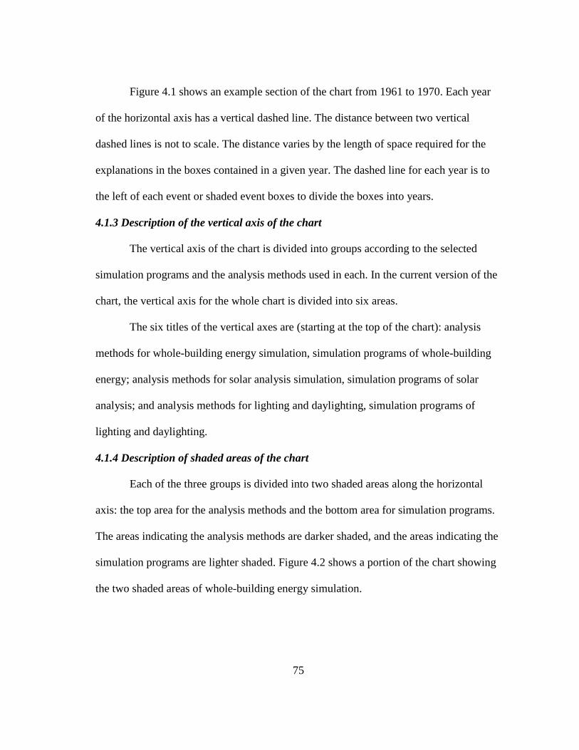
75

Figure 4.1 shows an example section of the chart from 1961 to 1970. Each year

of the horizontal axis has a vertical dashed line. The distance between two vertical

dashed lines is not to scale. The distance varies by the length of space required for the

explanations in the boxes contained in a given year. The dashed line for each year is to

the left of each event or shaded event boxes to divide the boxes into years.

4.1.3 Description of the vertical axis of the chart

The vertical axis of the chart is divided into groups according to the selected

simulation programs and the analysis methods used in each. In the current version of the

chart, the vertical axis for the whole chart is divided into six areas.

The six titles of the vertical axes are (starting at the top of the chart): analysis

methods for whole-building energy simulation, simulation programs of whole-building

energy; analysis methods for solar analysis simulation, simulation programs of solar

analysis; and analysis methods for lighting and daylighting, simulation programs of

lighting and daylighting.

4.1.4 Description of shaded areas of the chart

Each of the three groups is divided into two shaded areas along the horizontal

axis: the top area for the analysis methods and the bottom area for simulation programs.

The areas indicating the analysis methods are darker shaded, and the areas indicating the

simulation programs are lighter shaded. Figure 4.2 shows a portion of the chart showing

the two shaded areas of whole-building energy simulation.

76

Sim

ula

tio

n P

rogr

ams

of

Wh

ole

Bu

ildin

g En

ergy

An

alys

is M

eth

od

s fo

r W

ho

le B

uild

ing

Ener

gy

Sim

ula

tio

n

1966“Fortran IV programs to calculate radiant energy

interchange factors”(Mitalas & Stephenson)

1965The first use of

computers in the design and analysis of building

systems began(APEC Formed)

1965“An assessment of

common assumptions in estimating cooling loads

and space temperatures”

(Mitalas)

N3

A2

N3

Figure 4.2. Example: a portion of the chart showing the two shaded areas of whole

building energy simulation.

The shaded event boxes have shadows to clearly indicate that these boxes explain

simulation programs. The sizes of the shaded areas are dependent on the number of the

event boxes during each period. The event or the shaded event boxes in the chart may

have a small rounded box, a small rectangular box, or both types at the bottom of the

event boxes. The explanations of the small boxes are included in Table 4.1.

In the case of Figure 4.2, the event box in the dark area (i.e., the analysis method

section) indicates Mitalas evaluated the assumptions for cooling load calculations in

1965. Mitalas was a researcher at N3 (i.e., National Research Council Canada). This

study was related to RFM (i.e., response factor method). The shaded event boxes in the

77

light area (i.e., the simulation program section) indicate that the Automated Procedures

for Energy Consultants (APEC) started to use digital computers for designing and

analyzing building systems in 1965. In addition, in 1966, Mitalas and Stephenson, who

were researchers at N3, developed Fortran IV programs to calculate interchange factors

of radiant energy.

Figure 4.3 shows one example of an event box that has both a small, rounded box

and a small, rectangular box at the bottom.

1981The Custom WFM for Thermal-Load

Calculations in DOE-2

(Kerrisk)

WFML2

Figure 4.3. Example: small, rounded and rectangular boxes at the bottom of the event

box.

The small, rounded box in the lower left is labeled L2 to indicate Los Alamos

Scientific Laboratory or LASL (now Los Alamos National Laboratory or LANL). The

small, rectangular box at the lower right indicates Weighting Factor Method (WFM).

Figure 4.4 shows an arrow that connects two event boxes. The arrow between

event boxes indicates that the events, which are explained in the boxes, are related to

each other.

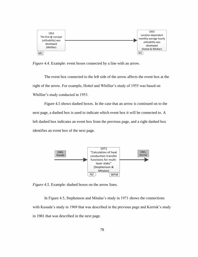
78

1953The first ф concept

(utilizability) was developed(Whillier)

1955Location-dependent

monthly average hourly utilizability was

developed(Hottel & Whillier)

M1 M1

Figure 4.4. Example: event boxes connected by a line with an arrow.

The event box connected to the left side of the arrow affects the event box at the

right of the arrow. For example, Hottel and Whillier’s study of 1955 was based on

Whillier’s study conducted in 1953.

Figure 4.5 shows dashed boxes. In the case that an arrow is continued on to the

next page, a dashed box is used to indicate which event box it will be connected to. A

left dashed box indicates an event box from the previous page, and a right dashed box

identifies an event box of the next page.

N2

1971“Calculation of heat conduction transfer functions for multi-

layer slabs”(Stephenson &

Mitalas)

WFM

1969, Kusuda

1981, Kerrisk

Figure 4.5. Example: dashed boxes on the arrow lines.

In Figure 4.5, Stephenson and Mitalas’s study in 1971 shows the connections

with Kusuda’s study in 1969 that was described in the previous page and Kerrisk’s study

in 1981 that was described in the next page.

79

Figure 4.6 shows the example of a diamond-shaped box. A diamond-shaped box

with a number signifies the classification of the analysis methods for lighting and

daylighting simulation.

1923Waldram diagrams for

calculating Sky component was

invented by Waldram(Hopkinson et al., 1966)

1

Figure 4.6. Example: a diamond box with a number on the left of the event box.

The number inside the diamond box is categorized as follows: 1. Graphical

methods; 2. Geometrical instruments; 3. Sky models; 4. Mathematical Formulae; 5.

Computer graphic techniques; 6. Daylight analysis tools; and 7. Tools that can calculate

the impact of daylighting strategies on energy consumption of buildings. These

categories were based on Kota and Haberl’s classification (Kota and Haberl, 2009). In

Figure 4.6, the diamond box with number one indicates Waldram’s diagram developed

in 1923 was one of graphical methods.

Figure 4.7 shows an example of a big, rounded box.

1967BIN method

(ASHRAE)

Figure 4.7. Example: a big, rounded box.

80

An example of a big, rounded box indicates an analysis method or simulation

program that does not meet the criteria used in the scope of this study. The criteria are:

(a) the simulation program is widely used in the U.S., (b) the program and its

documentation are available in the U.S. in English, (c) the simulation program or a

derivative of the program is still presently in use and supported, and (d) the analysis

method used in the simulation program has made a large contribution toward the

development of simulation in this area. In Figure 4.7, for example, the BIN method

introduced by ASHRAE in 1967 is not presently in use and supported for simulation.

4.1.5 Errors or discrepancies found from the previous studies or previous history

diagrams

Some of the historical facts from previous studies or previous history diagrams

have errors or discrepancies. Table 4.2 shows several of the errors or discrepancies

found from the previous studies.

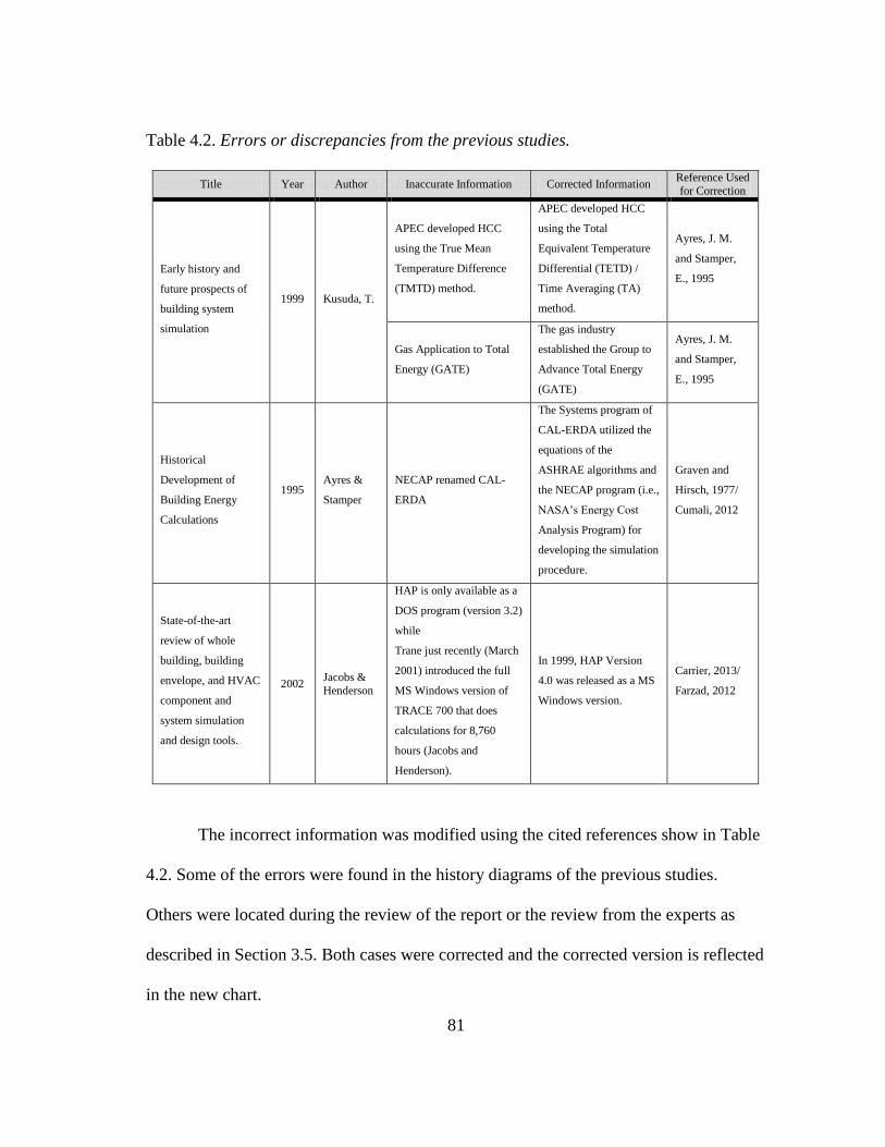
81

Table 4.2. Errors or discrepancies from the previous studies.

Title Year Author Inaccurate Information Corrected Information Reference Used

for Correction

Early history and

future prospects of

building system

simulation

1999 Kusuda, T.

APEC developed HCC

using the True Mean

Temperature Difference

(TMTD) method.

APEC developed HCC

using the Total

Equivalent Temperature

Differential (TETD) /

Time Averaging (TA)

method.

Ayres, J. M.

and Stamper,

E., 1995

Gas Application to Total

Energy (GATE)

The gas industry

established the Group to

Advance Total Energy

(GATE)

Ayres, J. M.

and Stamper,

E., 1995

Historical

Development of

Building Energy

Calculations

1995 Ayres &

Stamper

NECAP renamed CAL-

ERDA

The Systems program of

CAL-ERDA utilized the

equations of the

ASHRAE algorithms and

the NECAP program (i.e.,

NASA’s Energy Cost

Analysis Program) for

developing the simulation

procedure.

Graven and

Hirsch, 1977/

Cumali, 2012

State-of-the-art

review of whole

building, building

envelope, and HVAC

component and

system simulation

and design tools.

2002 Jacobs &

Henderson

HAP is only available as a

DOS program (version 3.2)

while

Trane just recently (March

2001) introduced the full

MS Windows version of

TRACE 700 that does

calculations for 8,760

hours (Jacobs and

Henderson).

In 1999, HAP Version

4.0 was released as a MS

Windows version.

Carrier, 2013/

Farzad, 2012

The incorrect information was modified using the cited references show in Table

4.2. Some of the errors were found in the history diagrams of the previous studies.

Others were located during the review of the report or the review from the experts as

described in Section 3.5. Both cases were corrected and the corrected version is reflected

in the new chart.

82

4.2 Four Methods to Utilize the New Comprehensive Genealogy Chart

This section describes four approaches or methods to effectively utilize the new

comprehensive genealogy chart. The approaches are divided by time period, analysis

method, simulation program, and organization or funding source.

4.2.1 Analysis by time period

The analysis by time period helps readers understand when the simulation

programs and their analysis methods were developed and includes selected background

or additional information about the simulation programs or the analysis methods created.

4.2.2 Analysis by analysis method

The analysis by analysis method presents the key analysis methods used in the

simulation programs. This approach explains why the analysis methods were developed,

who developed them, and how the analysis methods were developed.

4.2.3 Analysis by simulation program

The analysis by simulation program describes when the simulation programs

were developed, who developed them, why the simulation programs were developed,

and which analysis methods were used in the simulation programs.

4.2.4 Analysis by organization

The analysis by the organization or funding explains which organizations funded,

or contributed to the development of simulation programs, including their objectives and

conferences.

A more detailed description and discussion of the genealogy chart using the four

approaches will be presented in the next chapter.

83

4.3 Summary of Results

In this chapter, the format of new comprehensive genealogy chart was described.

The chart has six components, vertical and horizontal axes, and different shaded areas.

These features were explained in Sections 4.1.1 to 4.1.4. Errors and inaccurate

information discovered in the previous studies with respect to building simulation

programs and their analysis methods were presented in Section 4.1.5. The errors were

corrected, and these corrected errors were used in the new genealogy chart. Section 4.2

described the four methods to utilize the new comprehensive genealogy chart. The next

chapter, Chapter V, will include the analysis discussions and references for the chart.

84

CHAPTER V

DISCUSSION OF THE NEW GENEALOGY CHART

In this chapter, the new comprehensive genealogy chart is discussed using the

four approaches discussed in Chapter IV including: by time period, by analysis method,

by simulation program, and by organization. Figure 5.1 outlines these approaches.

Appendix AThe Comprehensive

Genealogy Chart

Section 5.1Table and

Discussion by Time Period

Section 5.2Table and

Discussion by Analysis Method

Section 5.3Table and Discussion

by Simulation Program

Section 5.4Table and Discussion

by Funding Organization

Chapter VISummary

and Future Work

Appendix BAnnotated

References used in the Comprehensive

Genealogy Chart

Figure 5.1. Structure of discussion of the comprehensive genealogy chart.

Each section is characterized using a summary table categorized by time period,

by specific analysis method, by specific simulation program, and by organization. The

summary tables are presented to help readers better understand the genealogy chart

shown in Appendix A.

85

In Section 5.1, the origins of the selected key analysis methods and computer

programs are described by time period. The historical background of the origins and

additional analysis methods are also noted. Table 5.1 presents the matrix of the

development of the selected analysis methods and computer programs, which are

classified by time period. The year indicates when the analysis methods or simulation

programs were first released. Section 5.2 explains the origins of the analysis methods

used in the selected simulation programs by the three groups (i.e., whole-building

analysis, solar energy analysis, and lighting and daylighting analysis simulation

programs). Table 5.2 shows the analysis methods classified by the three groups, the

parameters of the analysis methods, and the years when the analysis methods were

developed. Section 5.3 describes the origins of the simulation programs by the three

groups. The years when the simulation programs were released are indicated in Table

5.3. Section 5.4 historically explains the key organizations that contributed to the

development of the analysis methods or the simulation programs. Table 5.4 shows which

organization supports which simulation program or analysis method and the years when

the organizations were founded.

Appendix B provides major annotated references used in the chart. The

references are classified by the three groups and the analysis methods of each group.

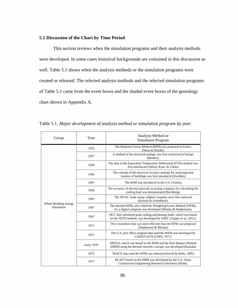
86

5.1 Discussion of the Chart by Time Period

This section reviews when the simulation programs and their analysis methods

were developed. In some cases historical backgrounds are contained in this discussion as

well. Table 5.1 shows when the analysis methods or the simulation programs were

created or released. The selected analysis methods and the selected simulation programs

of Table 5.1 came from the event boxes and the shaded event boxes of the genealogy

chart shown in Appendix A.

Table 5.1. Major development of analysis method or simulation program by year.

Group Year Analysis Method or

Simulation Program

Whole-Building Energy Simulation

1925 The Response Factor Method (RFM) was proposed in France

(Nessi & Nisolle)

1937 A method of the electrical analogy was first conceived in Europe

(Beuken).

1939 The idea of the Equivalent Temperature Differential (ETD) method was

first introduced (Alford, Ryan, & Urban)

1942 The concept of the electrical circuitry analogy for analyzing heat

transfer of buildings was first introduced (Paschkis)

1947 The RFM was introduced in the U.S. (Tustin)

1958 The accuracy of thermal network on analog computer for calculating the

cooling load was demonstrated (Buchberg).

1963 The HVAC loads using a digital computer were first analyzed

(Kusuda & Achenbach).

1967 The detailed RFM, also called the Weighting Factor Method (WFM),

for a digital computer was developed (Mitalas & Stephenson).

1967 HCC that calculated peak cooling and heating loads, which was based

on the TETD method, was developed by APEC (Tupper et al., 2011).

1971 The z-transform that was more efficient than the RFM was proposed

(Stephenson & Mitalas)

1971 The U.S. post office program that used the WFM was developed by

GARD/GATX (USPS, 1971)

Early 1970 NBSLD, which was based on the RFM and the Heat Balance Method

(HBM) using the thermal network concept, was developed (Kusuda)

1972 TRACE that used the WFM was released (Sowell & Hittle, 1995)

1977 BLAST based on the HBM was developed by the U.S. Army

Construction Engineering Research Laboratory (Hittle).

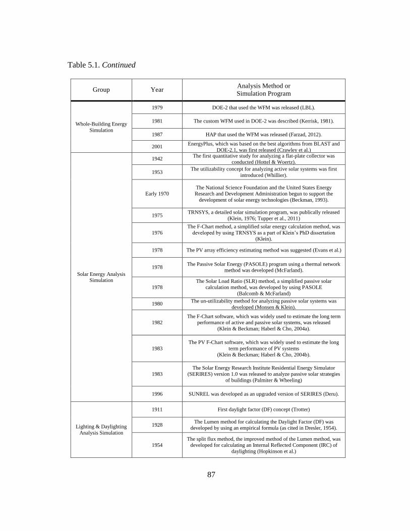
87

Table 5.1. Continued

Group Year Analysis Method or

Simulation Program

Whole-Building Energy

Simulation

1979 DOE-2 that used the WFM was released (LBL).

1981 The custom WFM used in DOE-2 was described (Kerrisk, 1981).

1987 HAP that used the WFM was released (Farzad, 2012).

2001 EnergyPlus, which was based on the best algorithms from BLAST and

DOE-2.1, was first released (Crawley et al.)

Solar Energy Analysis Simulation

1942 The first quantitative study for analyzing a flat-plate collector was

conducted (Hottel & Woertz).

1953 The utilizability concept for analyzing active solar systems was first

introduced (Whillier).

Early 1970 The National Science Foundation and the United States Energy Research and Development Administration begun to support the

development of solar energy technologies (Beckman, 1993).

1975 TRNSYS, a detailed solar simulation program, was publically released

(Klein, 1976; Tupper et al., 2011)

1976

The F-Chart method, a simplified solar energy calculation method, was

developed by using TRNSYS as a part of Klein’s PhD dissertation (Klein).

1978 The PV array efficiency estimating method was suggested (Evans et al.)

1978 The Passive Solar Energy (PASOLE) program using a thermal network

method was developed (McFarland).

1978

The Solar Load Ratio (SLR) method, a simplified passive solar

calculation method, was developed by using PASOLE

(Balcomb & McFarland)

1980 The un-utilizability method for analyzing passive solar systems was

developed (Monsen & Klein).

1982 The F-Chart software, which was widely used to estimate the long term

performance of active and passive solar systems, was released

(Klein & Beckman; Haberl & Cho, 2004a).

1983

The PV F-Chart software, which was widely used to estimate the long

term performance of PV systems

(Klein & Beckman; Haberl & Cho, 2004b).

1983 The Solar Energy Research Institute Residential Energy Simulator

(SERIRES) version 1.0 was released to analyze passive solar strategies

of buildings (Palmiter & Wheeling)

1996 SUNREL was developed as an upgraded version of SERIRES (Deru).

Lighting & Daylighting

Analysis Simulation

1911 First daylight factor (DF) concept (Trotter)

1928 The Lumen method for calculating the Daylight Factor (DF) was

developed by using an empirical formula (as cited in Dresler, 1954).

1954 The split flux method, the improved method of the Lumen method, was

developed for calculating an Internal Reflected Component (IRC) of

daylighting (Hopkinson et al.)

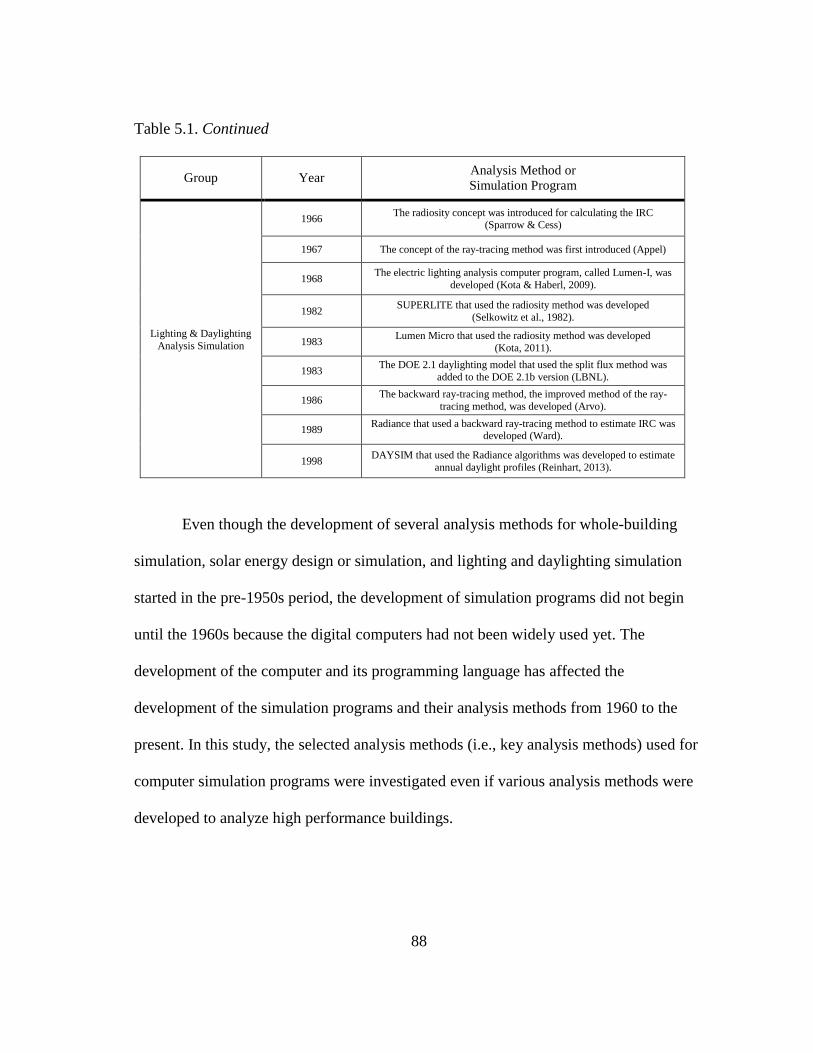
88

Table 5.1. Continued

Group Year Analysis Method or

Simulation Program

Lighting & Daylighting

Analysis Simulation

1966 The radiosity concept was introduced for calculating the IRC

(Sparrow & Cess)

1967 The concept of the ray-tracing method was first introduced (Appel)

1968 The electric lighting analysis computer program, called Lumen-I, was

developed (Kota & Haberl, 2009).

1982 SUPERLITE that used the radiosity method was developed

(Selkowitz et al., 1982).

1983 Lumen Micro that used the radiosity method was developed

(Kota, 2011).

1983 The DOE 2.1 daylighting model that used the split flux method was

added to the DOE 2.1b version (LBNL).

1986 The backward ray-tracing method, the improved method of the ray-

tracing method, was developed (Arvo).

1989 Radiance that used a backward ray-tracing method to estimate IRC was

developed (Ward).

1998 DAYSIM that used the Radiance algorithms was developed to estimate

annual daylight profiles (Reinhart, 2013).

Even though the development of several analysis methods for whole-building

simulation, solar energy design or simulation, and lighting and daylighting simulation

started in the pre-1950s period, the development of simulation programs did not begin

until the 1960s because the digital computers had not been widely used yet. The

development of the computer and its programming language has affected the

development of the simulation programs and their analysis methods from 1960 to the

present. In this study, the selected analysis methods (i.e., key analysis methods) used for

computer simulation programs were investigated even if various analysis methods were

developed to analyze high performance buildings.

89

5.1.1 Pre-1950s

In the pre-1950s period, specifically from 1600 and 1900, most fundamentals

(i.e., gas laws, heat properties, and thermodynamics) of HVAC systems were studied.

They scientifically contributed to the development of technology. Gas laws explained

the relations of temperature, volume, and pressure, and thermodynamics described the

relations of heat, work, and energy. The fundamental understanding allowed engineers to

create more efficient systems and predict energy performance (Donaldson et al., 1994).

In 1836 and 1850, Thomas Tredgold and Eugéne Péclet introduced heat transfer theory

for ventilating and heating systems through their books (Donaldson et al., 1994; Mao et

al., 2013). In 1894, Hermann Rietschel, a professor at the Technical University of Berlin

– Charlottenburg, proposed general procedures for the design of HVAC systems based

on the scientific fundamentals. The title of the published book was Guide to Calculating

and Design of Ventilating and Heating Installations (Donaldson et al., 1994).

The most important social issues in the pre-1950s period were World War I and

II, which spanned each from 1914 to 1918 and from 1939 to 1945. World War I and II

forced governments to promote energy conservation. People tried to save resources due

to the war, and it motivated engineers to create efficient methods to save energy (Shavit,

1995).

The development of a computer was also important event in the pre-1950s. In

1834, Charles Babbage designed a computing machine (i.e., called the Analytical

Engine) that became the basis of a current computer framework (Steitz, 2006; CHM,

2008). During World War I, mechanical calculators were developed to help engineers

90

better calculate the trajectory of artillery shells, whereas World War II saw the

development of punched-cards, the electronic calculators (i.e. ENIAC and EDVAC) and

the development of the first computers (i.e., COLOSSUS and MANIAC), which were

the foundation for all computers that followed (McCartney, 1999; Copeland, 2006). In

1946, John Mauchly and John Presper Eckert at the University of Pennsylvania

developed the Electrical Numerical Integrator And Calculator (ENIAC) sponsored by

the U.S. Army. The first digital calculator for a general purpose, ENIAC, was originally

developed for enhancing artillery target accuracy. However, ENIAC was used for

estimating weather prediction and wind tunnel calculations as well as military

experiments because World War II ended in 1945 (Bellis, 2013).

5.1.1.1 Discussion of Pre-1950s whole-building simulation

In order to estimate whole-building energy use, the fundamentals and essential

concepts for calculating cooling and heating loads were developed in the pre-1950s

period.

In 1897, Rolla Carpenter discussed time-dependent temperature to select a

radiator size in the American Society of Heating and Ventilating Engineers (ASHVE,

now ASHRAE) Transactions (Carpenter, 1897). This was the first study to be published

in the ASHVE Transactions for considering time-dependent temperature (Shavit, 1995).

In 1907, he used the Peclet equation developed in 1868 to estimate material conduction

by temperature difference with the coefficient of conductivity and the thickness of the

material (Carpenter, 1907). In 1913, Ralph C. Taggart first published the differential

equation in the ASHVE Transactions to estimate the required time to heat rooms by

91

using steam radiators. The differential equation was solved by an explicit approach

(Taggart, 1913; Shavit, 1995). The use of air conditioning increased the importance of

calculating heat gain and loss in buildings (Shavit, 1995). In 1935, F. Faust, L. Levine,

and F. Urban, engineers at the General Electric Corporation, calculated the cooling load

by using a time lag effect in a paper, titled “A rational heat gain method for the

determination of air conditioning cooling loads” (Faust et al., 1935). The time lag

accounted for the effect of wall’s thermal storage capacity. In other words, the time lag

concept accounted for time delay and heat amplitude reduction between an outer surface

and an inter surface of a wall (Faust et al., 1935; Alford et al., 1939). In 1939, J. Alford,

J. Ryan, and F. Urban, engineers at the General Electric Corporation, proposed a

decrement factor to visualize the wall’s thermal storage capacity (Alford et al., 1939).

Through World War II (1939-1945), people recognized the importance of

available resources. Researchers started to develop new methods for the building

performance computation (Shavit, 1995). In 1942, the concept of the electrical circuitry

analogy for analyzing heat transfer in buildings was first introduced by Victor Paschkis,

a research engineer at Columbia University (Paschkis, 1942; Paschkis and Baker, 1942;

Shavit, 1995). C. Beuken first conceived a method of the electrical analogy in Europe in

1937 and 1938 (as cited in Paschkis and Baker, 1942).

92

After World War II, researchers used analog computers5 for solving various

engineering problems. In 1948, Harold Johnson, a professor at University of California –

Berkeley, used this technology (i.e., analog circuitry) to analyze transient thermal

performance at inner surfaces of building walls (Johnson, 1948). The weighting factor

concept for the transient thermal behavior was introduced in his study (Johnson, 1948;

Shavit, 1995). In the same year, Charles Leopold, a consulting engineer, developed a

hydraulic analogue based on the electric analogy approach to accurately estimate

conduction, convection, radiation, and thermal storage behavior used for calculating a

cooling load (Leopold, 1948).

The most widely-used concept for calculating instantaneous heat gain through

walls and roofs was the Response Factor Method (RFM), first used by André Nessi and

Léon Nisolle, engineers at Ėcole Centrale Paris, in France in 1925 (Nessi and Nisolle,

1925; Haberl and Cho, 2004c). The RFM was first introduced in the U.S. in 1947 by

Arnold Tustin, who was a British professor at the University of Birmingham. This

method was published in an Electrical Engineering Journal (Tustin, 1947; Haberl and

Cho, 2004c).

Another transient heat gain calculation method, called the Equivalent

Temperature Differential (ETD) method, which was later used in the Total Equivalent

Temperature Differential (TETD)/Time Averaging (TA) method (Rees et al., 2000), was

5 Analog computers use continuous inputs (i.e., electrical circuits) to calculate problem variables described

using electrical voltages, whereas digital computers use discrete inputs using symbols such as numbers

and letters, which are described in programming languages (i.e., FORTRAN) (Dooijes and Peek, 2013;

Collins, 2013).

93

proposed by James Stewart at the Carrier Corporation in 1948 (Stewart, 1948). This

ETD method was based on the concept of the sol-air temperature method developed in

1944 by C. Mackey and L. Wright, professors at Cornell University (Mackey and

Wright, 1944, 1946). Mackey and Wright’s study referenced the solution of J. Alford, J.

Ryan, F. Urban proposed in 1939 (Alford et al., 1939; Mackey and Wright, 1944).

Mackey and Wright’s study assumed periodic cycles of steady state temperature on a

one-day basis for calculating heat gain through walls and roofs. This assumption caused

one of the limitations to accurately estimate heat gain of buildings (Kusuda, 1969).

5.1.1.2 Discussion of Pre-1950s solar energy analysis simulation

In this study, the origins of today’s solar thermal, solar PV, and passive solar

simulation programs were also investigated. In the pre-1950s period, active solar thermal

systems included solar collectors, storage units, and solar domestic hot water (SDHW)

systems. In terms of solar collectors, a flat-plate collector was widely used because this

type of collector is easier to build than other types of collectors. In 1885, Charles Tellier

set up and introduced the concept of a tilted, flat-plate collector, which heated ammonia,

with a solar water pumping system (Tellier, 1885). In 1909, H. Willsie developed a

horizontal, flat-plate collector that used a working fluid of sulphur dioxide to collect heat

for a heat engine operation (Willsie, 1909). In order to analyze a flat-plate collector,

Hoyt Hottel and B. Woertz first conducted a quantitative study in 1942 (Hottel and

Woertz, 1942). This method was the basis of the utilizability method introduced by

Austin Whillier in 1953 (Whillier, 1953a, 1953b).

94

5.1.1.3 Discussion of Pre-1950s lighting and daylighting simulation

In the pre-1950s period, sky models for calculating sky luminance and

daylighting analysis methods for calculating daylight illuminance in buildings started

being developed. These studies became the key methods of lighting and daylighting

simulation programs.

A sky model is one of important factors to estimate daylighting in a building

because both direct and diffuse daylight from the sun and sky come into a building. In

1921, Herbert Kimball and Irving Hand at the Weather Bureau in Washington D.C. first

measured sky luminance distribution (Kimball and Hand, 1921; Kota, 2011). In 1929,

Pokrowski developed a formula for calculating the luminance distribution of a cloudless

clear sky using Rayleigh scattering6. In 1942, P. Moon and D. Spencer developed an

empirical formula for calculating sky luminance distribution of an overcast sky (as cited

in Hopkinson et al, 1966; Kota, 2011).

Most daylightling calculation methods used in today’s simulation tools are

divided into a daylight factor (DF) method, a daylight coefficient (DC) method, and a

ray-tracing technique (Kota, 2011). The first study using the daylight factor was

conducted by Alexander Trotter in 1989 (as cited in Walsh, 1951). In 1928, H. G.

Fruhling developed the Lumen method to calculate the DF using an empirical formula

(as cited in Dresler, 1954).

6 Light’s elastic scattering. This was discovered by Lord Rayleigh who was an English physicist. This is

caused by the electric polarizability of particles. Diffuse radiation of sky is generated from this

phenomenon of sunlight in the sky (Rayleigh Scattering, 2013).

95

The methods for finding components of the daylight factor (DF) can be divided

into graphical and non-graphical methods. In 1923, P. Waldram developed the Waldram

diagram, which is a graphical method used for estimating the overall DF or a single DF

component (as cited in Hopkinson et al., 1966). In 1946, A. Dufton proposed daylight

protractors as a non-graphical method to calculate the DF (as cited in Hopkinson et al.,

1966).

5.1.2 1950s

In the 1950s, analog computers became widely used for building energy analysis.

The key analysis methods for solar, lighting and daylighting simulation programs were

also developed in the 1950s, which were based on selected methods developed prior to

this time.

In the 1950s, a programming language for digital computers was developed that

became widely used in the 1960s. In 1954, the International Business Machines

Corporation (IBM) developed FORmula TRANslator (FORTRAN), which was the first

high level programming language. This language was commercially released in 1957

(CHM, 2008). FORTRAN positively affected the availability of a digital computer in the

1960s because FORTRAN allowed the simulation developers to create a program on one

computer to be run on another computer, so multiple programs for simulation were soon

developed.

5.1.2.1 Discussion of 1950s whole-building simulation

In the 1950s, analog computers were widely used to study cooling and heating

loads. In 1954, H. Nottage and G. Parmelee, research engineers at the American Society

96

of Heating and Ventilating Engineers (ASHVE) Research Laboratory, used thermal

circuits on analog computers to analyze cooling and heating loads (Nottage and

Parmelee, 1954). In the same year, T. Willcox, C. Oergel, S. Reque, C. ToeLaer, and W.

Brisken, who were engineers at the General Electric Corporation, studied cooling loads

used in residential buildings using analog computers (Willcox et al., 1954). In 1955,

Harry Buchberg used an analog computer approach to study thermal behavior in simple

dwelling houses. His original study was his Master of Science thesis at University of

California – Los Angeles (UCLA) sponsored by the American Society of Heating and

Air-Conditioning Engineers (ASHAE, formerly ASHVE and now ASHRAE) (Buchberg,

1955). In 1958, Buchberg extended his previous study that was conducted in 1955 as an

associate professor at UCLA, which was also sponsored by the ASHAE. In the second

study, he demonstrated the accuracy of thermal network on analog computer for

calculating the cooling load (Buchberg, 1958).

In 1956, the RFM using rectangular pulses was developed by W. Brisken and S.

Reque who were engineers at the General Electric Corporation after the RFM was first

introduced in the U.S. by A. Tustin in 1947. In the next year, Paul R. Hill at the Langley

Aeronautical Laboratory of the National Adivosry Committee for Aeronautics (NACA,

now National Aeronautics and Sapce Administration (NASA)) first proposed the RFM

that uses triangular pulses more accuracy than rectangular pulses (Hill, 1957).

5.1.2.2 Discussion of 1950s solar energy analysis simulation

In 1953, the key analysis method for solar simulation program was developed.

Austin Whillier first proposed the utilizability concept for analyzing the ratio of the

97

incident solar radiation that reaches the surface of a solar system, thorough his Ph.D.

dissertation at the Massachusetts Institute of Technology (MIT), under Prof. Hoyt

Hottel’s direction (Whillier, 1953b). In 1955, Hottel and Whillier used Whillier’s

utilizability concept to develop the location-dependent, monthly-average hourly

utilizability concept (Hottel and Whillier, 1955; Beckman, 1993; Haberl and Cho,

2004a).

5.1.2.3 Discussion of 1950s lighting and daylighting simulation

In order to have a designated sky model, in 1955 the International Commission

on Illumination (CIE) selected Moon and Spencer’s formula as the standard to calculate

the overcast sky luminance distribution. This formula was developed in 1942 for

luminance distribuition of an average overcast sky (as cited in Hopkinson et al, 1966).

In order to develop a daylighting calculation method in buildings, A. Dresler

(1954) extended the Lumen method, developed by Fruhling in 1928, and especially

improved the method to calculate an Internal Reflected Component (IRC) of daylight

(Dresler, 1954). In the same year, R. Hopkinson, J. Longmore, and P. Petherbridge at the

Building Research Station in the U.K. developed the split flux method based on A.

Dresler, W. Arndt, and G. Pleijel (Hopkinson et al., 1954). This method calculated the

IRC using an empirical formula. In 1958, Hopkinson et al. created tables to calculate

DFs (Hopkinson et al., 1966).

5.1.3 1960s

In the 1960s, digital computers began to be substituted for analog computers

because digital computers were more convenient to program new problems and digital

98

computers using FORTRAN made it easier to describe the governing equations and

driving functions than the configurations required by analog computers. The scientific

application of digital computers was considerably improved by FORTRAN, the high

level programming language that was commercially released in 1957 by IBM.

In the early 1960s, the Union of Soviet Socialist Republics (USSR) intimidated

the U.S. with their nuclear weapon. As a response, researchers at the Building Research

Division (BRD) of the National Bureau of Standards (NBS) (now the Building and Fire

Research Laboratory (BFRL) of the National Institute of Standards and Technology

(NIST)) studied the indoor, thermal environmental conditions in high occupancy fallout

shelters using an IBM 7094 with FORTRAN (Kusuda, 1999). This study was one of the

first studies to use a digital computer to study the dynamic heat transfer in a building.

The Stanford Research Institute (SRI) reported building space heating and

cooling energy accounted for approximately 20% of the end-use consumption in 1968 in

the U.S (as cited in ASHRAE, 1975a). This report helped engineers recognize the

importance of energy saving in buildings, which helped motivate ASHRAE to begin its

research efforts in building energy simulations (ASHRAE, 1975a).

5.1.3.1 Discussion of 1960s whole-building simulation

In the early 1960s, analog computers were still used to analyze cooling and

heating loads in buildings like during the 1950s. In 1962, D. G. Stephenson and G. P.

Mitalas studied solar heat gain using an analog computer (Stephenson and Mitalas,

1962). In 1965, L. Nelson published one of the first detailed studies regarding the

99

interaction between envelope, equipment, and control systems of a building using an

analog computer (Nelson, 1965; Shavit, 1995).

In the 1960s, researchers started to use digital computers for estimating the

HVAC applications in buildings. In 1963, Tasami Kusuda and P. Achenbach’s study at

the NBS was one of the first to analyze the HVAC loads using a digital computer

(Kusuda and Achenbach, 1963). In 1967, G. P. Mitalas and D. G. Stephenson at the

National Research Council (NRC) Canada improved their own previous work that used

an analog computer in 1962 (Stephenson and Mitalas, 1962). Their study developed the

response factors for digital computers that became the basis for today’s instantaneous

heat gain analysis through walls and roofs of buildings (Mitalas and Stephenson, 1967;

Shavit, 1995).

Stephenson and Mitalas’s Response Factor Method (RFM) for calculating heat

gain through walls and roofs and Weighting Factor Method (WFM) for calculating

cooling loads (Mitalas and Stephenson, 1967; Stephenson and Mitalas, 1967) became the

important foundations toward the thermal performance development of whole-building

simulation computer programs (Shavit, 1995).

In 1967, Mitalas and J. G. Arseneault developed a FORTRAN IV program to

calculate heat gain through multi-layered slabs using the RFM of Mitalas and

Stephenson (Mitalas and Arseneault 1967; Kusuda, 1969). Mitalas and Arseneault used a

Laplace transform matrix introduced by Louis A. Pipes in 1957 (Pipes, 1957; Mitalas

and Arseneault 1967; Kusuda, 1969). Previously, Mackey and Wright’s study in 1944

100

employed Fourier series rather than the Laplace transform to calculate heat conduction

equations due to the low speed of computers (Mackey and Wright, 1944; Kusuda, 1969).

In 1969, Kusuda extended the RFM for calculating the response factors (RFs) for

curvatures of multi-layers (Kusuda, 1969). In the same year, Mitalas compared the

calculated results of the WFM with the measured data (Mitalas, 1969). Using the RFM

and the WFM, researchers and engineers could analyze the dynamic heat gain and

cooling loads through multi-layered walls and roofs to better design envelope and

HVAC systems in buildings.

In 1965, ASHRAE founded a Presidential Committee on Energy Consumption to

specifically address the calculations of heating and cooling loads with more accurate

computer methods. This committee reviewed the issues surrounding the development of

more accurate methods in detail and suggested further assignments to a task group,

called Task Group on Load Profiles, also founded in 1965. From 1965 to 1966, the

initial Task Group researched accurate methods and developed a diagram for calculating

building load profiles (Tull, 1971; Stamper, 1995). In 1966, the Task Group voted for

the ASHRAE budgets to fund energy calculation research projects and a new renamed

Task Group (Stamper, 1995). In 1967, the new Task Group known as the ASHRAE Task

Group on Energy Requirements (TGER) for Heating and Cooling Buildings held its first

meeting. Robert Tull, who was a previous ASHRAE president, became the first

chairman of the ASHRAE TGER (Tull, 1971; Stamper, 1995; Kusuda, 1999). In 1968

and 1969, ASHRAE TGER first presented two booklets that contained the computer

algorithms for the dynamic, hourly cooling and heating loads calculation methods and

101

methods for modeling secondary systems and plants. The first booklet on the loads

calculation was narrowly distributed to approximately 150 researchers and engineers at

the ASHRAE annual meeting in 1968 to receive comments from them (Lokmanhekim

ed., 1971; Tull, 1971). The final form of the booklet that contained the algorithms for the

pre-calculated WFM and the custom WFM was published in 1971 (Lokmanhekim ed.,

1971). The 3rd

edition of the booklet that included the algorithms for the WFM and the

HBM was presented in 1975 (ASHRAE, 1975a).

In the 1960s, the development of computer programs for calculating building

thermal performance began. In 1966 and 1967, Mitalas, Stephenson, and Arseneault who

were researchers at the NRC Canada developed FORTRAN IV programs to analyze

building thermal performance (Mitalas and Stephenson, 1966; Mitalas and Arseneault,

1967). FORTRAN IV was released by the IBM in 1962. In 1967, the group of consulting

engineers, called the Automated Procedures for Energy Consultants (APEC), developed

a computer program (i.e., HCC) that calculated peak cooling and heating loads for a

building. This program was based on the TETD/TA method introduced in ASHRAE

Guide and Data Book published in 1961 (ASHRAE, 1961; as cited in Ayres and

Stamper, 1995; Mao et al., 2013), which used the sol-air temperature method of Mackey

and Wright in 1944 and 1946 (Mackey and Wright, 1944, 1946). Many of the same

APEC members who developed the HCC program also participated in the formation of

the ASHRAE TGER (Tupper et al., 2011).

102

5.1.3.2 Discussion of 1960s solar energy analysis simulation

In 1963, the key analysis method (i.e., the utilizability method) for solar

simulation program was further developed (Liu and Jordan, 1963). Benjamin Liu and

Richard Jordan, professors at the University of Minnesota, developed the location-

independent, monthly average hourly utilizability method using Whillier’s utilizability

concept, developed in 1955 (Whillier, 1953a, 1953b).

5.1.3.3 Discussion of 1960s lighting and daylighting simulation

For a sky model, in 1965, R. Kettler developed a formula for luminance

distribution of a clear blue sky. The CIE selected Kettler’s formula for luminance

distribution of a clear blue sky as the standard for luminance distribution of a clear blue

sky with sun (as cited in Hopkinson et al., 1966).

For daylighting calculation methods in buildings, in 1966, E. Sparrow at the

University of Minnesota and R. Cess at the State University of New York at Stony

Brook introduced the radiosity concept in their book, entitled Radiation Heat Transfer

(Sparrow and Cess, 1966). In 1967, Arthur Appel at the IBM Research Center first

proposed the concept of ray tracing (Appel, 1967; Weghorst et al., 1984). These two

methods, the radiosity method and the ray tracing method became the basis of today’s

lighting and daylighting simulation programs.

For the simulation of lighting and daylighting, in 1968, the electric lighting

analysis computer program, called Lumen-I, was developed by David DiLaura, which

was based on point-by-point calculations. In 1970, DiLaura developed Lumen II that

103

improved the existing capabilities of Lumen I by adding the calculations for daylighting,

glare, and visual comfort (as cited in Kota and Haberl, 2009).

5.1.4 1970s

As a result of the oil crises (i.e., 1973 and 1979), the development of FORTRAN,

and the increasing availability of digital computers, more and more engineers began to

develop building thermal calculation methods and eventually whole-building simulation

programs (Ayres and Stamper, 1995). Engineers and researchers were finally able to

more easily apply the laws of thermodynamics to complex whole-building simulation

programs using mainframe computers with FORTRAN (Pedersen, 2009).

In 1970, the first symposium with respect to the use of computers for building

energy simulation was held at the National Bureau of Standards (NBS) in Gaithersburg,

Maryland. This symposium, entitled “Use of Computers for Environmental Engineering

Related to Buildings”, attracted approximately 400 architects, engineers, and scientists

from 12 countries. The NBS, ASHRAE, and the Automated Procedures for Energy

Consultants (APEC) sponsored this symposium. The 59 technical papers of this

symposium addressed issues including computer applications for building heat transfer

analysis, loads and energy calculations, HVAC system simulations, weather data, and

computer graphics (Kusuda ed., 1971).

5.1.4.1 Discussion of 1970s whole-building simulation

Several significant events occurred in the 1970s. First, in 1971, Stephenson and

Mitalas proposed the z-transform method that was more efficient than the Response

Factor Method (RFM) regarding speed and memory space of digital computers

104

(Stephenson and Mitalas, 1971). In 1975, the ASHRAE TGER published the 3rd

editions

of “Procedure for Determining Heating and Cooling Loads for Computerizing Energy

Calculations” and “Procedures for Simulating the Performance of Components and

Systems for Energy Calculations”, which were originally published in 1968 and 1969

(ASHRAE, 1975a, 1975b). These publications helped researchers and engineers quickly

learn the basic knowledge of whole-building simulation programs, which accelerated the

development of whole-building energy simulation (Sowell and Hittle, 1995).

In the late 1960s, the NBS used the state-of-the-art digital computer to estimate

heat conduction of fallout shelters in underground. Based on this work, in the early

1970s, Kusuda at the NBS proposed the National Bureau of Standards Load

Determination (NBSLD) program that used the RFM and the Heat Balance Method

(HBM) to analyze building thermal performance (i.e., heating and cooling loads)

(Stamper, 2001; Wright, 2003). This NBSLD program was developed for calculating

cooling loads, excluding HVAC systems and plants. Later, this program was improved

for calculating annual energy use with simple HVAC systems in one zone (Kusuda,

1999). In 1976, the FORTRAN algorithms of NBSLD were publically released to help

engineers develop their own simulation programs according to their needs. Some of the

algorithms that came from ASHRAE TGER’s book (ASHRAE, 1975a) were corrected

in the NBSLD algorithms book (Kusuda, 1976). The U.S. Army Construction

Engineering Research Laboratory (CERL) used these algorithms including the HBM to

develop CERL’s first building simulation program, called as TASS. In 1977, CERL

developed the Building Load Analysis and System Thermodynamics (BLAST) program

105

using the modifications to CERL’s first simulation program (i.e., TASS) and a new

FORTRAN code. In 1979, BLAST 2.0 was released. The HBM concept of NBSLD and

BLAST is now the basis for today’s public domain program, EnergyPlus (Walton,

2001).

In 1971, the U.S. Post Office released the post office program to analyze, design,

or remodel U.S. Post Office facilities (Lokmanhekim, 1971; USPS, 1971). Researchers

at the General American Research Division (GARD) of the General American

Transportation Corporation (GATX), which was a subcontractor of Post Office facilities,

developed a building shadow calculation program under the direction of Metin

Lokmanhekim. The GARD/GATX developed the U.S. Post Office program based on the

ASHRAE TGER report about the shadow program and the ASHRAE TGER algorithms

that used the weighting factor method (WFM) (USPS, 1971; Ayres and Stamper, 1995;

Kusuda, 1999). As a result, the U.S. Post Office program became the first public domain

program for whole-building simulation accounting for cooling and heating loads, HVAC

systems, plants, and economic analysis (USPS, 1971; Haberl and Cho, 2004c).

In the late 1970s, Zulfikar O. Cumali and the Computation Consultants Bureau

(CCB) developed the CAL-ERDA code based on the loads sub-program code used in the

Post Office Program (Cumali, 2013). The name of the CAL-ERDA program came from

the names of the sponsors: the California (CAL) Energy Commission and the United

States Energy Research and Development Administration (ERDA). CAL-ERDA was an

improvement over the Post Office program because the code of the Post Office program

was a monolithic that required recompilation for each subroutine, whereas CAL-ERDA

106

was speed up by recompiling the code. The CCB also developed the Building

Description Language (BDL) for CAL-ERDA, which was the first user-friendly

computer input language (i.e., familiar terminology), for controlling the load, systems,

plant, and economic sub-programs of the program (Graven and Hirsch, 1977; Cumali,

2013). The Lawrence Berkeley Laboratory (LBL, now Lawrence Berkeley National

Laboratory (LBNL)), the Argonne Nation Laboratory (ANL), and the Los Alamos

Scientific Laboratory (LASL, now Los Alamos National Laboratory (LANL)) also

contributed to the development of CAL-ERDA (Graven and Hirsch, 1977).

In 1976, CAL-ERDA was released. In the same year, the California Energy

Commission (CEC) and the ERDA sponsorship for CAL-ERDA ended and the ERDA

was integrated into the U.S. Department of Energy (US DOE) (Birdsall et al., 1990).

About this same time when M. Lokmanhekim moved from the GARD/GATX in Illinois

to the LBL in California, he brought his skills from the development of the Post Office

program to the LBL to accelerate the development of CAL-ERDA (Kusuda, 1999). The

LOADS program of CAL-ERDA was developed based on the ASHRAE algorithms

published in 1975. The SYSTEMS program of CAL-ERDA utilized the equations of the

ASHRAE algorithms and the NECAP7 program (i.e., the National Aeronautics and

Space Administration (NASA)’s Energy Cost Analysis Program) for developing the

simulation procedure (Graven and Hirsch, 1977).

7 NECAP was developed by the GARD/GATX under the sponsorship of the NASA in 1975 by improving

the Post Office program (Henninger ed., 1975; Sowell and Hittle, 1995). NECAP consisted of six

computer programs: Response Factor Program, Data Verification Program, Thermal Load Analysis

Program, Variable Temperature Program, System and Equipment Simulation Program, and Owning and

Operating Cost Program (Henninger ed., 1975).

107

In 1978, DOE-1, a slightly enhanced version of CAL-ERDA, was released by

CCB, LBL (now LBNL), LASL (now LANL), and ANL (ANL, 1978 as cited in LASL,

1980; Cumali, 2013). The US DOE Office of Buildings and Community Systems

supported the development of DOE-1 (Birdsall et al., 1990). Zulfikar Cumali, Ender

Erdem, Robert Grave, and Metin Lokmanhekim led the development of the BDL of

DOE-1 (LASL, 1980). In 1979, LBL improved the central plant algorithms of DOE-1

and released DOE-2 (Ayres and Stamper, 1995). In 1979 and 1980, DOE-2.0a and DOE-

2.1a were released by LBL and LASL. In the new programs, a new BDL had been

created for the DOE-2 series to more easily control the LOADS analysis program, the

SYSTEMS program, the PLANT program, and the ECONOMICS analysis program.

Frederick Buhl, James Hirsch, and Mark Roschke helped design the BDL of the DOE-2

series. Frederick Buhl was the principal researcher for the LOADS program, James

Hirsh for the SYSTEMS program, Steven Gates for the PLANT program, Frederick

Winkelmann for the ECONOMICS and LOADS programs, and Mark Roschke for the

DOE-2 Solar Simulator, which was called the Component Based Simulator (CBS) for

active solar systems (LASL, 1980).

In terms of the proprietary programs regarding whole-building simulation in the

1970s, in 1972, the Trane company released Trane Air Conditioning Economics

(TRACE) direct version. TRACE was derived from the post office program developed in

1971 (Sowell and Hittle, 1995). In 1977, TRACE 77 version was released (Tupper et al.,

2011).

108

In addition to the hourly whole-building simulation programs, performance-

based (i.e., minute-by minute) simulation programs were also developed. In the early

1960s, Nelson at Honeywell, Inc. started the effort to study dynamic performance of

buildings, HVAC systems, and control systems within them, using an analog computer

(Nelson, 1965). In 1978, Gideon Shavit at Honeywell, Inc. developed the performance-

based simulation program, BLDSIM, using a digital computer (as cited in Shavit, 1995).

Digital computers made it possible to solve any ordinary differential equations and non-

linear relationship to better analyze the high-frequency dynamic performance of HVAC

control systems in a building (Shavit, 1995).

5.1.4.2 Discussion of 1970s solar energy analysis simulation

In the early 1970s, the Solar Energy Laboratory (SEL) at the University of

Wisconsin-Madison (UWM) and the Solar Energy Applications Laboratory (SEAL) at

Colorado State University (CSU) began to study solar energy technologies supported by

the National Science Foundation and the United States Energy Research and

Development Administration (ERDA) (now the U.S. Department of Energy (US DOE))

(Beckman, 1993; Tupper et al., 2011). The CSU team planned to build a solar energy

test house, and needed a flexible simulation program to find the various design options

before the test house was built. Therefore, the UWM suggested a modular program for

flexible analysis, called the Transient Systems Simulation (TRNSYS) program (Klein,

1976; Beckman, 1993). Sanford A. Klein, a graduate student at the University of

Wisconsin-Madison, introduced the FORTRAN program, TRNSYS, through his PhD

study (Klein, 1976; Beckman, 1993). In 1975, TRNSYS was publically released, and

109

Klein finished his dissertation in 1976 (Tupper et al., 2011). Since then TRNSYS has

become a widely used modular or component-based program. Originally, TRNSYS was

developed for solar thermal simulations, but has also made a major contribution to

building energy simulation programs, PV analysis, and other analysis such as hydrogen

production analysis (Athienitis, et al., 2012).

For simplified solar energy calculations, in 1977, William. A. Beckman, Sanford.

A. Klein, and John. A. Duffie published the F-Chart method, which was a simplified set

of correlations based on thousands of simulations using TRNSYS (Klein, 1976;

Beckman et al., 1977).

In 1978 to further develop the utilizability method suggested in 1953 by Whillier

(Whillier, 1953a, 1953b), Klein developed the monthly-average daily utilizability

function that improved upon Liu and Jordan’s daily utilizability study in 1963 (Klein,

1978). In 1979, Manual Collares-Pereira at the University of Chicago and Ari Rabl at the

Solar Energy Research Institute (SERL, now National Renewable Energy Laboratory

(NREL)) developed long term average energy models using the daily utilizability

correlations in order to estimate different types of solar collectors such as flat-pate

collectors, compound parabolic concentrators (CPC), and tracking collectors for east-

west, polar, and two-axis tracking axis (Collares-Pereira and Rabl, 1979). Collares-

Pereira and Rabl’s study was supported by the US DOE. In 1980, J. C. Theilacker and

Klein proposed a new correlation method that simplified and improved the accuracy of

Klein’s correlation method that was developed in 1978. This method was also applicable

to surfaces facing the equator like Klein’s method, and it added more correlations for

110

surfaces shaded by overhangs and vertical surfaces facing east and west orientations

(Theilacker, 1980; Klein and Beckman, 1984; Theilacker and Klein, 1980; Jones and

Wray, 1992).

For photovoltaic (PV) system analysis, in 1978, D. L. Evans, W. A. Facinelli,

and R. T. Otterbein studied hybrid / PV thermal component models. A PV array

efficiency estimating method was suggested in this study (Evans et al., 1978; Klein and

Beckman, 1984).

For passive solar system analysis, in 1978, Robert D. McFarland at Los Alamos

Scientific Laboratory (LASL, now Los Alamos National Laboratory (LANL)) developed

the Passive Solar Energy (PASOLE) program using a thermal network method

(McFarland, 1978). In the same year, the Solar Load Ratio (SLR) method was proposed

by John Douglas Balcomb and R. D. McFarland (Balcomb and McFarland, 1978). The

Solar Load Ratio (SLR) method, a simplified passive solar calculation method, used

correlation parameters generated from thousands of runs with PASOLE, which is similar

to the relationship of the F-Chart method and TRNSYS. In 1980, another passive solar

method for estimating the useful amount of solar energy for passive solar heating loads

in building structure, called the un-utilizability method, was developed by W. A.

Monsen and Klein (Monsen and Klein, 1980).

In summary, during the 1970s, major solar energy analysis studies were

conducted under the US DOE’s support. The most widely used solar simulation

program, TRNSYS, was developed in 1975 based on a modular approach for flexibility.

The simplified solar energy calculation method, the F-Chart method, was developed in

111

1977 using TRNSYS. The previously developed utilizability method for estimating the

ratio of the incident solar radiation that reaches the surface of a solar system was further

developed in 1978, 1979, and 1980. A PV array efficiency estimating method was

developed in 1978. In the same year, the passive solar energy analysis program,

PASOLE, was developed. The simplified passive solar energy calculation method, the

SLR method, was also developed in 1978 using PASOLE. Another passive solar energy

calculation method, called the un-utilizability method for estimating the solar energy

amount above the critical solar level for calculating heating loads stored in building

structure, was developed in 1980.

5.1.4.3 Discussion of 1970s lighting and daylighting simulation

Graphical methods for calculating the DF were continuously developed after P.

Waldram developed the Waldram diagram in 1923. In 1979, Millet proposed the

Graphic Daylight Design Method (GDDM) to estimate the overall DF regarding the

standard CIE overcast sky. In 1980, Millet extended the study to include a clear sky (as

cited in Moore, 1985).

For glare analysis, in 1972, the Building Research Station (BRS) in the U.K. and

Cornell University proposed the Daylight Glare Index (DGI) to estimate glare, which

was an improvement on the BRS glare equation from 1950 (as cited in Kota, 2011). In

1979, H. D. Einhorn proposed a formula that contributed to the development of the CIE

Glare Index (CGI) (Einhorn, 1979; Wienold and Christoffersen, 2006).

For lighting and daylighting computation methods, in 1975 and 1976, DiLaura

who previously developed Lumen I and Lumen II in 1968 and 1970, respectively,

112

proposed efficient computation methods for calculating direct and reflected component

illuminance and visual comfort, which were used for Equivalent Sphere Illumination

(ESI) (DiLaura 1975, 1976). In 1980, DiLaura established Lighting Technologies Inc.

This company later released Lumen III in 1981 (Moore, 1985; Kota and Haberl, 2009).

5.1.5 1980s

In the 1980s, microcomputers became widely used for building energy

simulation programs. Unfortunately, the accuracy of simulation results using

microcomputers was less than the accuracy of simulation results using mainframe

computers. The main reason for this was that microcomputers used simplified

calculation methods compared to the detailed methods of the mainframe computers.

Even though microcomputers had lower accuracy, engineers preferred to use

microcomputers because mainframe computers were expensive and difficult to use and

engineers had trouble understanding the complete operating systems of mainframe

computers (Kusuda, 1985). Eventually, by the late 1980s, microcomputers (i.e., personal

computers) became powerful enough to run mainframe computer-based simulation

programs such as DOE-2 and BLAST.

Another trend of the 1980s was that existing the whole-building simulation

programs were updated and revised, rather than developing new analysis methods for

simulation programs (Tupper et al., 2011). On the other hand, the analysis methods for

solar simulation programs, lighting and daylighting simulation programs were

continuously developed.

113

5.1.5.1 Discussion of 1980s whole-building simulation

The weighting factor method (WFM), which was developed in the mid-1960s,

was improved for use in various room types in a building. In 1979, Zulfikar O. Cumali

and his associates (i.e., the CCB) developed the mathematical method of an upgraded

WFM, called a custom WFM (Cumali et al., 1979; Cumali, 2013). In 1981, the custom

WFM method used in the DOE-2.1 program was described in detail (Kerrisk, 1981;

Kerrisk et al., 1981). The original WFM (i.e., precalculated WFM) used precalculated

input data representing typical buildings (i.e., light, medium, and heavy construction),

whereas the custom WFM employed actual input data representing various buildings

(Kerrisk et al., 1981).

In the 1980s, there were also updates and improvements to whole-building

simulation programs8. In 1981, BLAST 3.0, which was the upgraded version of BLAST

2.0 from 1979, was released (Herron et al., 1981). In addition, DOE-2.1a was released in

1981 (LASL, 1981). During the remainder of the 1980s new versions of DOE-2 were

released including: DOE-2.1b in 1982, DOE-2.1c in 1984, and DOE-2.1d in 1989 (LBL,

1982, 1984, 1989). The details of new versions will be further discussed in Section

5.3.1.1 and 5.3.1.2.

8 In the 1980s, many engineering offices did not have mainframe computers, and the speed of personal

computers was slow. Therfore, A Simplified Energy Analysis Method (ASEAM), which was a public

domain program, was widely used during the period because ASEAM could run on small and slow

computers (PNNL, 1990; Jacobs and Henderson, 2002; Landsberg, 2013). ASEAM used a modified bin

method for loads calculation and the system and plant algorithms of DOE-2 for system energy calculation

(Cane, 1979; Knebel, 1983; PNNL, 1990; Landsberg, 2013). W. S. Fleming & Associates, Inc. developed

ASEAM. The US DOE’s Federal Energy Management Program (FEMP) supported the development of

ASEAM (PNNL, 1989, 1990).

114

In terms of the development of the proprietary programs for whole-building

simulation, in 1989, TRACE 600, which was the upgraded version of TRACE 77

(originally released in 1977) was released (Tupper et al., 2011). Another proprietary

whole-building energy simulation program developed by the Carrier Company was the

Hourly Analysis Program (HAP). In 1987, HAP version 1.0 was released, which was a

new enhanced version of the Commercial Load Estimating and Bin Opcost analysis

programs, which were developed by the Carrier Company. In 1989, HAP version 2.0

was released which used ASHRAE’s load calculation methods (Farzad, 2012).

To improve the documentation of whole-building energy calculation methods, in

the late 1980s, ASHRAE developed the annotated guide book for HVAC systems and

equipment that updated the previous ASHRAE book, “Procedures for Simulating the

Performance of Components and Systems for Energy Calculations” (Yuill, 1990). This

new annotated guide included new literature about mathematical models and computer

algorithms for HVAC systems and equipment.

In summary, in the 1980s, public domain (i.e., BLAST and DOE-2.1) and

proprietary whole-building simulation programs (i.e., TRACE and HAP) were improved

and updated. The upgraded WFM, called the custom WFM, was developed and used in

DOE-2.1. The mathematical theory and computer algorithms of this method were

introduced in 1979 and 1981. ASHRAE published the annotated guide book in 1990,

including mathematical models and computer algorithms for HVAC systems and

equipment.

115

5.1.5.2 Discussion of 1980s solar energy analysis simulation

For analyzing the performance of direct gain solar heating system, in 1981, W.

A. Monsen, S. A. Klein, and W. A. Beckman at the SEL of the UWM used the un-

utilizability method, which was previously proposed by Monsen and Klein in 1980, to

calculate the performance of thermal storage walls. In the same year, Klein, Monsen, and

Beckman also proposed a simplified procedure for analyzing the performance of thermal

storage walls using correlation parameters and tabulated weather data (Jones and Wray,

1992). For further developing the utilizability method suggested in 1953, Clark, Klein,

and Beckman developed a simplified algorithm in 1983 for digital computers to

calculate the hourly utilizability function for analyzing the solar radiation of active solar

heating systems. Also, in 1983, the F-Chart program, a simplified solar energy analysis

program, was released for use as a FORTRAN program. This program adopted the

utilizability and un-utilizability concepts for designing and analyzing active and passive

solar heating systems (Klein and Beckman, 2001a).

For analyzing the performance of PV systems, in 1980, D.L. Evans, W. A.

Facinelli, and L. P. Koehler at Arizona State University proposed a simplified, non-

computer based procedure to size PV arrays and battery storage to satisfy electrical loads

(Evans et al., 1980). In 1981, M. D. Siegel, Klein, and Beckman at the SEL of the UWM

also proposed a simplified method to analyze PV system performance using monthly-

average calculation (Siegel et al., 1981). Finally, in 1984, D. R. Clark, Klein, and

Beckman at the SEL of the UWM developed a method to analyze the long-term average

performance of PV systems (Clark et al., 1984). This method was used in the PV F-

116

Chart program to calculate the annual performance of PV systems. The user manual of

the program, which detailed the analysis of the method developed by Clark, Klein, and

Beckman in 1984, was published in 1985 (Klein and Beckman, 2001b).

In the 1980s, two simplified solar energy analysis programs (i.e., long-term,

monthly analysis programs), the F-Chart software and the PV F-Chart software, were

released. The F-Chart software is widely used to calculate the long term performance of

active and passive solar systems, and the PV F-Chart software is widely used to calculate

the long term performance of PV systems. In 1982, F-Chart versions 1.0 through 4.1

were released for mainframe computers using the FORTRAN programming language. In

1983, F-Chart version 5 was released for microcomputers, which was programmed in

BASIC. In the same year, the PV F-Chart computer program was first released. In 1985,

PV F-Chart version 3.3 was released for microcomputers that used Disk Operating

System (DOS). All the F-Chart and PV F-Chart programs were developed by the SEL of

the UWM (Haberl and Cho, 2004a, 2004b).

For passive solar system analysis, in 1983, Larry Palmiter and Terry Wheeling at

the Ecotope Group developed the Solar Energy Research Institute Residential Energy

Simulator (SERIRES) Version 1.0, a FORTRAN program, to analyze passive solar

strategies used in residential and small commercial. The development of SERIRES was

founded through a contract with the Solar Energy Research Institute (SERI) (now the

National Renewable Energy Laboratory, (NREL)). Ron Judkoff, Bob O'Doherty, David

Simm, and David Wortman were technical monitors of SERI. SERIRES was released for

117

mainframe computers programmed in FORTRAN 66 in 1983 buildings (Palmiter and

Wheeling, 1983).

In summary, the utilizability and un-utilizability methods were further developed

in 1983 and 1981 respectively, and a simplified analysis method for the performance of

PV systems was developed in 1984. The two simplified solar energy analysis programs

(i.e., long-term, monthly analysis programs), the F-Chart software for active and passive

solar strategies and the PV F-Chart software for PV strategies, were released in 1983 and

1985. The SERIRES simulation program for analyzing passive solar strategies used in

residential and small commercial buildings was released in 1983.

5.1.5.3 Discussion of 1980s lighting and daylighting simulation

In regards to daylighting calculation methods in buildings, in 1982, the radiosity

computer algorithms, which were based on the radiosity concept introduced in 1966,

were developed to calculate the Internal Reflected Component (IRC) in buildings

(Modest, 1982; Selkowitz et al., 1982; Kim et al., 1986). In addition, the lighting and

daylighting simulation program, SUPERLITE (Selkowitz et al., 1982) that used the

radiosity algorithms was also developed (Hitchcock and Carroll, 2003).

Other daylighting calculation methods in buildings were also developed during

this period. In 1983, P. R. Tregenza and I. M. Waters developed the concept of a

Daylight Coefficient (DC) method (Tregenza and Waters, 1983). The DC method was

used to calculate the illuminance distributions inside buildings according to the sky

luminance conditions present at a given moment. In 1986, James Arvo developed a

backward ray-tracing method following the concept of ray-tracing, which was originally

118

developed by Arthur Appel in 1967 (Appel, 1967). The backward ray tracing method

provided an improved solution for exactly calculating the indirect diffuse reflection,

which had not been previously solved (Arvo, 1986).

In terms of a sky model for a daylighting model, in 1987, K. Matsuura developed

a new formula for the sky model. This formula was used for calculating luminance

distribution of a clear turbid sky and for an intermediate sky condition (as cited in Kota,

2011).

In the 1980s, several new versions of lighting and daylighting analysis programs

were developed. In 1981, David L. DiLaura and Lighting Technologies, Inc. developed

Lumen III, which was upgraded from the previous Lumen II program (Moore, 1985;

Kota, 2011). In Lumen III, flux transfer algorithms were provided, which were

previously developed by D. L. DiLaura and Gregg A. Hauser in 1978 (DiLaura and

Hauser, 1978; Moore, 1985). In 1982, DiLaura and Lighting Technologies, Inc.

developed a new daylighting program for microcomputers named Energy, which was

also marketed by Lighting Technologies, Inc. (Moore, 1985). In 1983, DiLaura and

Lighting Technologies, Inc. developed the Lumen Micro program that used radiosity

algorithms (Kota, 2011). Also, in 1983, the DOE-2.1b version was released, which

added a daylighting analysis model using the split flux method. In the early 1980s,

SUPERLITE was developed at the Lawrence Berkeley Laboratory (LBL, now Lawrence

Berkeley National Laboratory (LBNL)), which used the radiosity algorithms to analyze

the IRC (Selkowitz et al., 1982). In 1989, Radiance was first released by Gregory J.

Ward at the LBL (Ward, 1994). Radiance, which was developed on the UNIX platform

119

is an advanced lighting and daylighting simulation program for analyzing color (i.e.,

renderings) and illuminance of building inside and outside light (EERE, 2011c).

Radiance used a backward ray-tracing method to estimate the IRC. In 1990, Radiance

versions 1.2 and version 1.3 were released (LBNL, 2013).

In summary, for daylighting calculations in buildings, radiosity algorithms were

developed in 1982. Advanced daylighting calculation methods, including the DC method

and the backward ray-tracing method, were introduced in 1983 and 1986. In the 1980s,

several new versions of the previously developed and new programs for lighting and

daylighting simlation were developed (i.e., Lumen III, Lemen Micro, DOE-2.1

daylighting model, SUPERLITE, and Radiance).

5.1.6 1990s

In the 1990s, as personal computers continued to improve, the decreased price

and improved speed and memory of the computers made it possible for engineers to use

detailed engineer programs on their personal computers in their offices (Ayres and

Stamper, 1995). Also, in 1985, Microsoft (MS) Windows, which added a graphical user

interface (GUI) to the underlying DOS operating system, was released. In a similar

fashion to the Apple’s GUI, MS Windows GUI also helped to accelerate the use of

personal computers by the general public.

The improvement and enhancement of existing simulation programs also

continued during the 1990s. Most of the improvements were focused on the development

of the graphical user interface and more sophisticated analysis procedures (Ayres and

Stamper, 1995; Sowell and Hittle, 1995). These improvements added new algorithms to

120

better integrate existing procedures, and in some cases, provided optimized solution

schemes (Sowell and Hittle, 1995).

5.1.6.1 Discussion of 1990s whole-building simulation

For more efficient and rigorous cooling load calculation, in 1997, Jeffrey D.

Spitler, Daniel E. Fisher, and Curtis O. Pedersen at University of Illinois at Urbana-

Champaign (UIUC) proposed the Radiant Time Series (RTS) method for calculating

peak cooling load. This new method was an improvement over the previous

CLTD/SCL/CLF, TETD/TA, and TFM methods (Spitler et al., 1997; ASHRAE, 2001).

In terms of the development of simulation programs, the first version of DOE

2.1e and DOE-2.1e-087 were released by LBL in 1993 and 1995 (Winkelmann et al.;

1993; LBNL and JJH, 1998). In the early 1990s, engineers of James J. Hirsch and

Associates (JJH), LBNL (the new name of LBL from 1995 to the present), and the

Electric Power Research Institute (EPRI) began to develop DOE-2.2, a new version of

DOE-2.1. In 1996, PowerDOE, the first graphical interface program using DOE-2.2, was

created by JJH. In 1999, eQUEST version 1.0, another graphical interface program using

DOE 2.2 was released by JJH. While the development of PowerDOE stopped in 2001

due to funding difficulty, eQUEST has been continuously developed until today (as cited

in Tupper et al., 2011).

In 1996, the U.S. Department of Energy (US DOE) and the U.S. Department of

Defense (US DOD) started to develop a new whole-building simulation program, called

EnergyBase, later designated as EnergyPlus (Crawley et al., 1997). EnergyPlus

combined the best features of DOE-2 released by LBNL in 1979, BLAST and IBLAST

121

released by U.S. Army Construction Engineering Research Laboratory (CERL) and

University of Illinois in 1977 and 1994 (Crawley et al., 1999). The alpha version of

EnergyPlus was developed and tested internally in 1998, and a beta version of

EnergyPlus was released to be tested by engineers outside the development circle in

1999 (Crawley et al., 1999). Due to the development of the new simulation program

(i.e., EnergyPlus), the funding for further improvements to BLAST and DOE-2.1 was

discontinued (Tupper et al., 2011).

The development of the two most widely used proprietary whole-building

simulation programs, TRACE and HAP, continued. The Carrier Company released HAP

version 3.0 in 1993 and version 4.0 in 1999. HAP version 4.0 was the first version to be

developed for the Microsoft Windows (Farzad, 2012). The Trane Company released

TRACE 700 in 1998, which was their first Windows version (Tupper et al., 2011).

In respect to whole-building energy calculation methods documentation, in 1996,

ASHRAE, who recognized the importance of documentation for building energy

analysis methods, published another annotated guide for load calculation models and

algorithms, following the previously published annotated guide for HVAC equipment

published in 1990 (Spitler, 1996). In 1993 and 1998, ASHRAE issued two new toolkits

for secondary and primary HVAC systems (Brandemuehl et al., 1993; ASHRAE 1998).

These new toolkits contained algorithms, models and executable FORTRAN code to

help simulation software developers better understand and create new programs (Spitler,

1996; Pedersen et al., 2003). The toolkits replaced the earlier ASHRAE book, named

“Procedures for Simulating the Performance of Components and Systems for Energy

122

Calculations” published by the ASHRAE TGER in 1975 (ASHRAE, 1975b; Spitler,

1996)). The new toolkits also included updates based on ASHRAE’s literature search,

which was conducted in the annotated guide for HVAC equipment issued in 1990

(Spitler, 1996).

In summary, regarding whole-building energy calculation methods

documentation, ASHRAE, who recognized the importance of documentation for

building energy analysis methods, published in 1966 an updated annotated guide for load

calculation models and algorithms, following the previously published annotated guide

for HVAC equipment that was published in 1990. In the 1990s, the development of the

whole-building simulation programs continued. The first version of DOE 2.1e and The

087 version of DOE-2.1e were released by LBL in 1993 and 1995. In 1996, the U.S.

Department of Energy (US DOE) and the U.S. Department of Defense (US DOD)

started to develop a new whole-building simulation program, called EnergyBase, later

designated as EnergyPlus. The development of the two most widely used proprietary

whole-building simulation programs, TRACE and HAP, continued as well. The Carrier

Company respectively released HAP versions 3.0 and 4.0 in 1993 and 1999. The Trane

Company released TRACE 700 in 1998.

5.1.6.2 Discussion of 1990s solar energy analysis simulation

In 1993, Klein and Beckman released the F-Chart program version 6.17W and

the PV F-Chart program version 3.01W. Both versions were now compatibly with the

MS Windows operating system (Haberl and Cho, 2004a, 2004b). In 1996, the SEL of the

123

UWM also released TRNSYS version 14.2, which was the first MS Windows

compatible version (as cited in Tupper et al., 2011).

In 1996, the SERIRES version 1.0, which was originally developed by the

Ecotope Group under the contract with the Solar Energy Research Institute (SERI) (now

the National Renewable Energy Laboratory (NREL)) in 1983, was upgraded and

released as SUNREL by Colorado State University and NREL (Deru, 1996). One of

upgrades was to make the format of the program more flexible with respect to future

improvements and to be compatible with visual user interfaces (Deru et al., 2002).

5.1.6.3 Discussion of 1990s lighting and daylighting simulation

From 1991 to 1997, the Radiance program was updated each year (i.e., version

2.0 in 1991, version 2.1 in 1992, version 2.3 in 1993, version 2.4 in 1994, version 2.5 in

1995, version 3.0 in 1996, and version 3.1 in 1997) (LBNL, 2013). In 1998, Reinhart

proposed DAYSIM using the Radiance algorithms as a lighting and daylighting analysis

simulation program that can estimate annual daylight profiles (Reinhart, 2013).

In terms of a sky model for a daylighting model, Richard Perez, R. Seals, and J.

Michalsky at the State University of New York developed a new sky model for all

weather conditions in 1993 (Perez et al., 1993). This model was adopted shortly after by

the Radiance and DAYSIM programs (Kota, 2011).

5.1.7 From 2001 to present

Recently, growing concerns about climate change have led to an effort to reduce

CO2 emissions from fossil fuel-burning power plants that supply electricity to buildings.

Therefore, building standards and codes, for example, ASHRAE Standard 189.1-2009

124

and ASHRAE Standard 189.1-2011 published in 2009 and 2011 respectively, and the

International Green Construction Code (IGCC) issued in 2012, have been created for

high performance buildings to reduce energy use and CO2 emissions from fossil fuel-

fired power plants. In such standards and codes, building energy simulation is one of

severed compliance paths for a user to prove their proposed design consumes less energy

annually than a similar building built to the prescriptive cod standards (Tupper et al.,

2011).

The improvement and enhancement of existing simulation programs also

continued. Fixing existing bugs and having new simulation features were the main

reasons for further development of the simulation programs.

5.1.7.1 Discussion of whole-building simulation from 2001 to present

In 2001, the first version of EnergyPlus was released after the alpha and beta

testing of EnergyPlus was completed in the late 1990s (Crawley et al., 1999).

EnergyPlus is a public domain program, which was designed to be a modular, well-

structured code. EnergyPlus is based on the best algorithms from several of the previous

building simulation programs (i.e., BLAST, IBLAST, and DOE-2.1). After the first

release, EnergyPlus was improved and updated by the national laboratories and third-

party developers, under sponsorship by the US DOE. EnergyPlus version 1.1 was

released in 2003, version 1.2 in 2004, version 1.3 and 1.4 in 2006, version 2.0 and 2.1 in

2007, version 2.2 and 3.0 in 2008, version 3.1 and 4.0 in 2009, version 6.0 in 2010,

version 7.0 in 2011, version 7.1 and 7.2 in 2012, and version 8.0 in 2013(EERE, n.d.;

125

EERE, 2010; EERE, 2011e; EERE, 2012; EERE, 2013b). The details of all the different

versions will be noted in Section 5.3.1.1.

Due to the focus on the development of EnergyPlus, funding for improving

DOE-2.1 was terminated. Instead of the US DOE funding for improvements to DOE-2.1,

DOE-2.2, a new proprietary version of DOE-2.1 developed in the late 1990s, has been

continuously improved for the capabilities and fixing bugs of DOE-2.2 until today.

eQUEST, the graphic interface version of DOE-2.2, also has been upgraded by James J.

Hirsch and Associates (JJH). In 2001, 2003, 2005, 2007, and 2010, eQUEST versions

2.17c, 3.4, 3.55, 3.61b, and 3.64 were respectively released (as cited in Tupper et al.,

2011; JJH, 2009). The details of the different versions will be described in Section

5.3.1.3.

The two most popular proprietary whole-building simulation programs, TRACE

and HAP were also widely used in the 2000s. TRACE and HAP can be used to calculate

building loads, building energy use, and size HVAC systems (Jacobs and Henderson,

2002; Farzad, 2012). TRACE, developed by the Trane Company in 1972, has been

continuously updated and released until today (i.e., Trace 700 full version in 2001, Trace

700 version 4.1 in 2002, Trace 700 version 6.0 in 2006, Trace 700 version 6.2 in 2008,

and Trace 700 version 6.2.10 in 2013) (Tupper et al., 2011; Trane, 2013). HAP,

developed by the Carrier Company in 1987, also has been continuously improved until

today (i.e., version 4.1 in 2002, version 4.2 in 2003, version 4.3 in 2006, version 4.4 in

2008, version 4.5 in 2010, version 4.6 in 2012, and version 4.7 in 2013) (Carrier, 2013).

126

The details of TRACE and HAP versions will be described in Section 5.3.1.4 and

5.3.1.5.

TRNSYS, which was released by Klein and the SEL in 1975, was originally

developed to analyze active solar heating systems. TRNSYS can be also used to simulate

HVAC systems using its component-based or modular approaches. The solution

algorithms of TRNSYS were more rigorous than the solution algorithms of whole-

building energy simulation programs such as BLAST and DOE-2.1. However, the

models of whole-building simulation programs for calculating conventional cooling and

heating loads were more detailed (Sowell and Hittle, 1995). TRNSYS was updated and

widely used in the U.S (i.e., version 15 in 2001, version 16 in 2004, version 17 in 2010,

and version 17.1 in 2012). The details of TRNSYS versions will be further discussed in

Section 5.3.1.6.

To improve the documentation of whole-building energy calculation methods, in

2002, ASHRAE published a toolkit for building load calculations, developed by C. O.

Pedersen, D. E. Fisher, R. J. Liesen, and R. K. Strand (Pedersen et al., 2003). The

ASHRAE toolkit for building loads replaced the ASHRAE TGER’s book about

procedures for determining heating and cooling loads issued in 1975 (ASHRAE, 1975a;

Pedersen et al., 2003). In additon, the new toolkit was based on the more recent literature

research from ASHRAE’s annotated guide for load calculation models and algorithms

written by Spitler in 1996 (Spitler, 1996).

In summary, from 2001 to the present, improvements and enhancements to

existing simulation programs were conducted to mostly fix existing bugs and bring in

127

new features. In 2001, the first version of EnergyPlus was released after the alpha and

beta testing of EnergyPlus were completed in the late 1990s. After the first release,

EnergyPlus was improved and updated. eQUEST, TRACE, HAP, and TRNSYS were

also upgraded and enhanced by their developers.

5.1.7.2 Discussion of solar energy analysis simulation from 2001 to present

Since 2001, the user manuals of the F-Chart program and the PV F-Chart

program, published in 1983, were updated. New Windows versions of the F-Chart

program and the PV F-Chart program were also released in 2001 (Klein and Beckman,

2001b).

In 2002, Michael Deru, Ron Judkoff, and Paul Torcellini of NREL publically

released a new version of SUNREL. In 2004, SUNREL version 1.14 was released.

SUNREL is used almost exclusively to simulate passive solar technologies in small

buildings (Deru et al., 2002). SUNREL can be used to design “…moveable insulation,

interior shading control, energy-efficient windows, thermochromatic glazings, Trombe

walls, water walls, phase change materials, and rockbins.” (Deru et al., 2002, p.1).

5.1.7.3 Discussion of lighting and daylighting simulation from 2001 to present

After 2001, new methods for estimating daylighting performance, the Daylight

Autonomy (DA) and the Useful Daylight Illuminance (UDI) index, were developed

(Nabil and Mardaljevic, 2006). These methods were then used in DAYSIM to estimate

daylight profiles.

Since 2001, Radiance and DAYSIM that use the Radiance algorithms have been

continuously improved until today (i.e., DAYSIM version 1.3 in 2002, version 2.0 in

128

2003, version 2.1 in 2005, and version 3.X in 2010; Radiance version 3.4 in 2002,

version 3.5 in 2003, version 3.7 in 2005, version 3.9 in 2008, version 4.0 in 2010, and

version 4.1 in 2011) (LBNL, 2013; Reinhart, 2013). The details of Radiance and

DAYSIM versions will be further discussed in Section 5.3.3.1.1 and 5.3.3.1.2.

In 2004, DElight, a lighting and daylighting simulation program, was added to

EnergyPlus version 1.2. The DElight version 1.x series used the daylighting algorithms

of DOE-2.1. DElight version 2.0 was updated to use the radiosity algorithms of

SUPERLITE. The 2.0 version of DElight was included with EnergyPlus version 1.2,

which was released in 2004 (Hitchcock and Carroll, 2003; EERE, n.d.). The DElight

version 2.0 included algorithms to estimate complex fenestration systems (CFS)

(Hitchcock and Carroll, 2003).

5.1.8 Summary

Section 5.1 discussed the development of the analysis methods and the

simulation programs (i.e., whole-building energy simulation, solar energy analysis

simulation, and lighting and daylighting analysis simulation) by period: pre-1950s,

1960s, 1970s, 1980s, 1990s, and from 2001 to present. Appendix A shows the

comprehensive genealogy chart that is referenced in the discussions of Section 5.1.

Significant historical events such as World War I (1914-1918) and World War II

(1939-1945), the development of digital computers and computer programming

language (1950s), and repeated oil crises (1967, 1973, and 1979) have had a major

impact on the development of key analysis methods and the origins of the simulation

programs that are now used to simulate annual building energy use.

129

In the pre-1950s period, most of the fundamentals (i.e., gas laws, heat transfer

properties, and thermodynamics) of HVAC systems were studied and published that

significantly contributed to the development of today’s technology. Also, during this

same period, researchers and engineers developed the essential methods for: calculating

dynamic heat gain and building loads (i.e., cooling and heating loads) used in whole-

building energy simulation programs; calculating solar heating performance prediction

used in solar energy analysis design and simulation programs; and for analyzing

internally reflected illuminance used in lighting and daylighting simulation programs.

During the 1950s, analog computers became widely used to study the behavior of

dynamic heat gain/loss and the response of heating, ventilating, and air conditioning

(HVAC) systems. From the 1960s to the present, advanced digital computers and

analysis methods suitable for the digital computers were developed and became widely

used. Digital computers were substituted for analog computers because the digital

computer is more convenient to program, and the methods used in digital computers

made it easier and quicker to describe the governing equations and driving functions

than the methods used in analog computers. Finally, the scientific application of the

digital computer was considerably improved by the FORTRAN programming language,

a high level programming language that was commercially released in 1957 by IBM.

FORTRAN also allowed computer codes written on one computer to be run on another

computer by a different analyst, which accelerated the availability of simulation

programs. As a result, the concept of analog computers and the capabilities of digital

computers significantly contributed to the development of whole-building, solar energy,

130

lighting and daylighting simulation programs. Currently, almost all computer simulation

programs in use today continued to be written in the FORTRAN programming language.

Section 5.2, which follows, will discuss the comprehensive genealogy chart

shown in Appendix A by analysis method.

5.2 Discussion of the Chart for Tracing Specific Analysis Methods

A multitude of analysis methods are used in today’s whole-building simulation,

solar analysis simulation, and lighting and daylighting simulation programs. One way to

discuss these methods is to trace each method according to analysis type.

In general, whole-building simulation programs such as DOE-2 and BLAST

were composed of four major sections: loads, systems, plants, and economics (Sowell

and Hittle, 1995). In this study, the analysis methods for calculating building cooling

loads used in whole-building simulation programs are the main focus, with less of an

emphasis on systems, plant and economics.

Solar energy analysis programs evaluate the performance of systems that are

designed to collect and use solar radiation for thermal or electricity conversion. In this

study, the methods for estimating the solar heating performance prediction are the main

focus, with less of an emphasis on passive cooling methods or solar-driven cooling

simulations.

Historically, lighting and daylighting simulation programs have used three

components in order to calculate the daylight coming through a window or skylight: the

Sky Component (SC), the External Reflected Component (ERC), and the Internal

Reflected Component (IRC). For this study, the methods for IRC are primarily traced

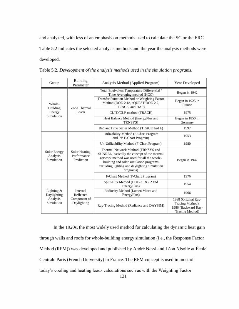
131

and analyzed, with less of an emphasis on methods used to calculate the SC or the ERC.

Table 5.2 indicates the selected analysis methods and the year the analysis methods were

developed.

Table 5.2. Development of the analysis methods used in the simulation programs.

Group Building

Parameter Analysis Method (Applied Program) Year Developed

Whole-

Building

Energy

Simulation

Zone Thermal

Loads

Total Equivalent Temperature Differential /

Time Averaging method (HCC) Began in 1942

Transfer Function Method or Weighting Factor

Method (DOE-2.1e, eQUEST/DOE-2.2,

TRACE, and HAP)

Began in 1925 in

France

CLTD/CLF method (TRACE) 1975

Heat Balance Method (EnergyPlus and

TRNSYS)

Began in 1850 in

Germany

Radiant Time Series Method (TRACE and L) 1997

Solar Energy

Analysis

Simulation

Solar Heating

Performance

Prediction

Utilizability Method (F-Chart Program

and PV F-Chart Program) 1953

Un-Utilizability Method (F-Chart Program) 1980

Thermal Network Method (TRNSYS and

SUNREL, basically the concept of the thermal

network method was used for all the whole-

building and solar simulation programs

excluding lighting and daylighting simulation

programs)

Began in 1942

F-Chart Method (F-Chart Program) 1976

Lighting &

Daylighting

Analysis

Simulation

Internal

Reflected

Component of

Daylighting

Split-Flux Method (DOE-2.1&2.2 and

EnergyPlus) 1954

Radiosity Method (Lumen Micro and

EnergyPlus) 1966

Ray-Tracing Method (Radiance and DAYSIM)

1968 (Original Ray-

Tracing Method),

1986 (Backward Ray-

Tracing Method)

In the 1920s, the most widely used method for calculating the dynamic heat gain

through walls and roofs for whole-building energy simulation (i.e., the Response Factor

Method (RFM)) was developed and published by André Nessi and Léon Nisolle at Ėcole

Centrale Paris (French University) in France. The RFM concept is used in most of

today’s cooling and heating loads calculations such as with the Weighting Factor

132

Method or the Transfer Function Method for DOE-2.1e, DOE 2.2/eQUEST, TRACE,

and HAP, the CLTD/CLF method for TRACE, the Heat Balance method for EnergyPlus

and TRNSYS, and the Radiant Time Series Method for TRACE.

In the 1940s, the origin of the Resistance-Capacitance (RC) network analysis

method (i.e., the thermal network method) used in solar and whole-building simulation

programs was first introduced by Victor Paschkis, a research engineer at Columbia

University. This thermal network concept is used in all solar energy simulation

programs, as well as whole-building energy simulation programs. In the 1950s, the most

important method (i.e, the utilizability method) for calculating the performance of solar

heating systems used in solar energy design or simulation programs was developed by

Austin Whillier at the MIT. The utilizability method is used today in detailed solar

energy simulation programs such as TRNSYS and in simplified solar energy design

programs such as the F-Chart and the PV F-Chart program.

In the 1950s and 1960s, the origins of the Inter Reflected Component (IRC)

calculation method (i.e., the split flux method, the radiosity method, and the ray tracing

method) for daylighting simulation were developed. In 1954, the split flux method was

proposed by R. Hopkinson, J. Longmore, and P. Petherbridge at the Building Research

Station in the U.K. In 1966, E. Sparrow at the University of Minnesota and R. Cess at

the State University of New York at Stony Brook introduced the radiosity concept in

their book, entitled Radiation Heat Transfer. In 1967, Arthur Appel at the IBM Research

Center first proposed the concept of ray tracing.

133

Today, the split flux method is used in whole-building energy simulation

programs such as DOE-2.1e, DOE 2.2/eQUEST, and EnergyPlus as a daylighting model.

The radiosity method is used in Lumen Micro and in EnergyPlus as a daylighting

module. The ray tracing method is also used in a detailed lighting and daylighting

simulation program including rendering such as Radiance.

5.2.1 The analysis methods of whole-building energy simulation

In Section 5.2.1, the origins of cooling load calculations used in building

simulation programs were described. Various methods for calculating commercial (i.e.,

non-residential) building cooling and heating loads9 have been developed (Mao et al.,

2013). However, in order to more rigorously calculate building loads over long periods

such as one year, rigorous hourly approaches were required that used digital computers

(ASHRAE, 1997).

In this study, the analysis methods for cooling load calculations used in today’s

whole-building energy simulation programs were included: The Total Equivalent

Temperature Difference (TETD) / Time Averaging (TA) method, the Cooling Load

Temperature Difference (CLTD) / Cooling Load Factor (CLF) method, the Transfer

Function Method (TFM), and the Radiant Time Series (RTS) method for calculating

peak cooling load; the Weighting Factor Method (WFM) and the Heat Balance Method

(HBM) for calculating time-varying cooling load for energy analysis (ASHRAE, 1997,

2009; Rees et al., 2000; Smith, 2011).

9 In this study, the origins of the analysis methods for cooling loads were analyzed rather than heating

loads. Procedures for calculating cooling loads are basically the same to those for calculating heating loads

with some exceptions (ASHRAE, 2009).

134

Cooling load calculations are mainly categorized by four variables: heat gain,

cooling load, heat extraction rate, and cooling coil load. Heat gain means the entered or

generated instantaneous heat gain in a space through walls, roofs, and windows. Cooling

load indicates the instantaneous heat that has to be removed in a space to keep constant

air temperature and humidity. Cooling load is affected by a time delay effect (i.e., the

thermal storage effect). Heat extraction rate is the same to the space cooling load if the

space air temperature is constant. The space heat extraction rate covers the effect of a

slight cyclic variation or swing of space temperature. Finally, cooling coil load is the

instantaneous heat removal from the cooling coil and additional system loads such as

heat gain due to fan, duct, outdoor air heat, and outdoor air moisture (ASHRAE, 2009).

In this study, the origins of heat gain and cooling loads were analyzed. Figure 5.2 and

Figure 5.3 show the diagrams of the ASHRAE handbook published in 1997 and 2009.

The diagram (see Figure 5.2) of the past ASHRAE handbook published in 1997 contains

the TETD/TA method (ASHRAE, 1961), the TFM (McQuiston and Spitler, 1992), and

the CLTD/CLF method (Rudoy and Duran, 1975).

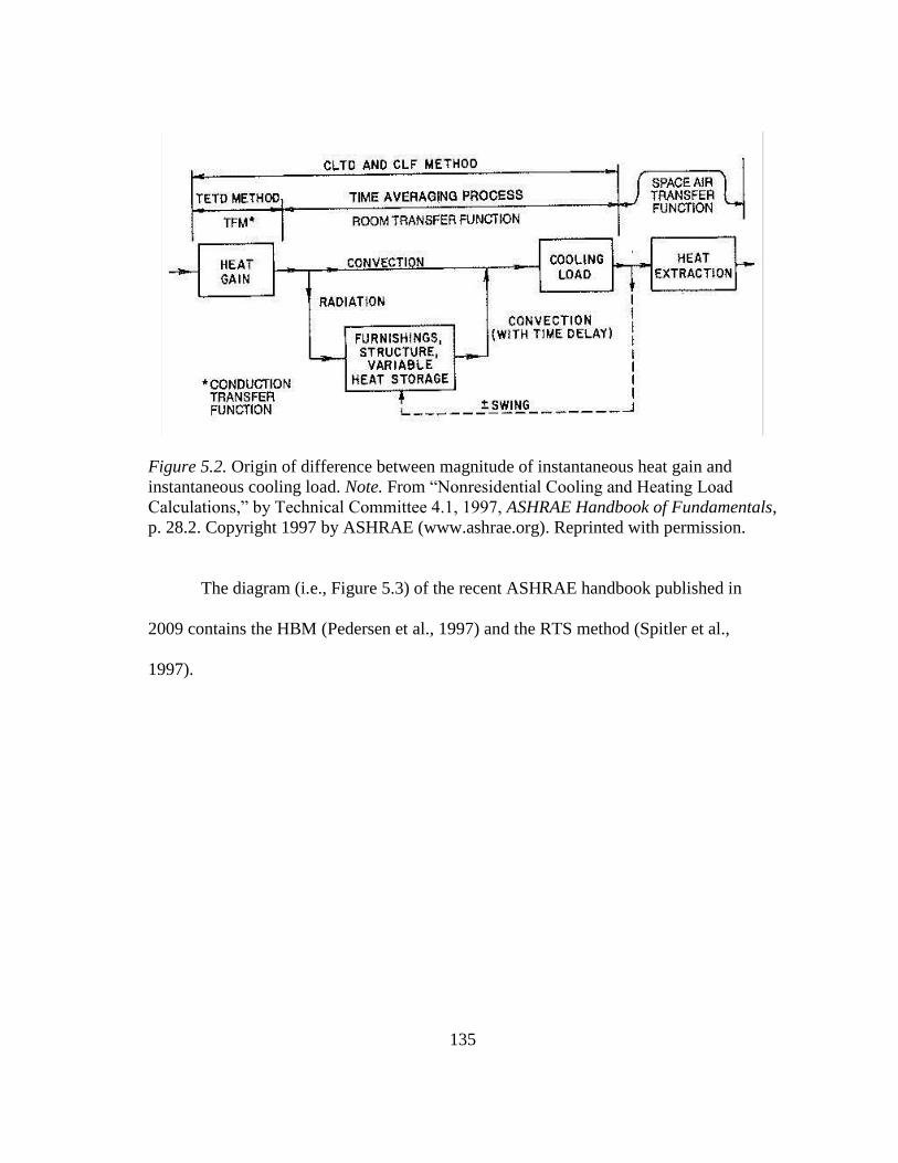
135

Figure 5.2. Origin of difference between magnitude of instantaneous heat gain and

instantaneous cooling load. Note. From “Nonresidential Cooling and Heating Load

Calculations,” by Technical Committee 4.1, 1997, ASHRAE Handbook of Fundamentals,

p. 28.2. Copyright 1997 by ASHRAE (www.ashrae.org). Reprinted with permission.

The diagram (i.e., Figure 5.3) of the recent ASHRAE handbook published in

2009 contains the HBM (Pedersen et al., 1997) and the RTS method (Spitler et al.,

1997).

136

Figure 5.3. Origin of difference between magnitude of instantaneous heat gain and

instantaneous cooling load. Note. From “Nonresidential Cooling and Heating Load

Calculations,” by Technical Committee 4.1, 2009, ASHRAE Handbook of Fundamentals,

p. 18.2. Copyright 2009 by ASHRAE (www.ashrae.org). Reprinted with permission.

.

Figure 5.2 and Figure 5.3 also indicate which analysis method is categorized in

the variable. The TETD method of the TETD/TA method, the Conduction Transfer

Functions (CTFs) of the WFM or the TFM, and the Conduction Time Series (CTS) of

the RTS method are used to calculate the heat gain. The TA method of the TETD/TA

method, the Weighting Factors (WFs) of WFM or TFM, and the Radiant Time Factors

(RTFs) of the RTS method are used for calculating the cooling load. The CLTD/CLF

method and HBM are used for calculating the heat gain and the cooling load at the same

time. Air temperature WFs of WFM or TFM is used for calculating the heat extraction

rate.

137

5.2.1.1 Total equivalent temperature difference (TETD) / Time averaging (TA) method

The TETD/TA10

method allowed building engineers to estimate approximate

heat gains by using tabulated TETD values of walls and roofs, or near equivalents

(ASHRAE, 1997). This method was first developed to analyze the transient aspects of

solar radiation and time delay by the thermal storage effect (McQuiston and Spitler,

1992). The heat gain using the TETD/TA method is obtained from the overall heat

transfer coefficient, U, and the equivalent temperature difference known as TETD

calculated by the sol-air temperature variation, decrement factors, and time lags

according to the type of construction of the walls and roofs (Threlkeld, 1970; McQuiston

and Spitler, 1992; ASHRAE, 1997). This heat gain method is considered a first order

Response Factor Method (i.e., decrement factors and delay factors) (McQuistion and

Spitler, 1992).

In the TETD/TA method, cooling load is calculated by using a Time Averaging

(TA) method in order to convert heat gain to cooling load. The TA method accounts for

a thermal storage effect or the radiant effect of heat gain (McQuiston and Spitler, 1992).

A thermal storage effect accounts for interior surfaces of a room that absorb and store

some radiation portion of heat gain. The absorbed and stored heat is later released to the

air in a room with the effect of time delay as convective heat unless the room surfaces

perfectly absorb or release heat (Kusuda and Powell, 1972). One of the limitations of the

TETD/TA method is that the TETD/TA does not provide a rigorous technique for

defining the TA period (i.e., time delay for cooling load). When the users of the

10 The TETD is used for calculating heat gain, and the TA is used for calculating cooling load.

138

TETD/TA method decide the TA period, the decision is based on users’ experience

(McQuiston and Spitler, 1992).

The development of TETD/TA is shown in the first shaded area from the top in

Figure A.2. An abbreviation, TT, in the small, rectangular boxes indicates the TETD/TA

method at the bottom of the event boxes. In 1944, C. Mackey and L. Wright, professors

at Cornell University, used the concept of sol-air temperature (called equivalent

temperature in England), decrement factors, and time lag to calculate periodic heat

transfer for homogeneous walls dealing with solar heat gain (Mackey and Wright, 1944).

This study was later extended to composite walls (Mackey and Wright, 1946). Mackey

and Wright’s studies were based on the studies proposed by F. Faust et al. and J. Alford

at al. at the General Electric Corporation in 1935 and 1939 (Faust et al., 1935; Alford et

al., 1939; Mackey and Wright, 1942). In 1935, F. Faust et al. calculated heat gain

through walls by considering a time lag and solar effect in their paper (Faust et al.,

1935). The time lag accounted for the effect of wall’s thermal storage capacity. In other

words, time lag concept accounted for time delay and heat amplitude reduction between

an outer surface an inter surface of a wall (Faust et al., 1935; Alford et al., 1939). In

1939, J. Alford et al. proposed a decrement factor to visualize the wall’s thermal storage

capacity (Alford et al., 1939).

The TETD method of the TETD/TA method was outlined and tabled for

calculating heat gain of practical walls by J. Stewart at the Carrier Corporation in 1948

based on Mackey and Wright’s study in 1944 (Stewart, 1948; Threlkeld, 1970). Finally,

the TETD/TA method using the TA was introduced to calculate cooling load in the

139

ASHRAE Guide and Data Book (now ASHRAE Handbook of Fundamentals) published

in 1961 (ASHRAE 1961; Mao et al., 2013). Even though the TETD/TA was developed

as a manual method at first, this method has also been used as a computer procedure

(McQuiston and Spitler, 1992). For example, the HCC program developed by APEC in

1967 used the TETD/TA method (Ayres and Stamper, 1995).

5.2.1.2 Transfer function method (TFM) or weighting factor method (WFM)

The TFM or the WFM was derived from the Heat Balance Method (HBM). In

other words, energy balance equations are used to determine weighting factors (Cumali

et al., 1979; Kerrisk, 1981). The transfer function concept is utilized in this method to

connect heat gain to cooling load and to connect cooling load to heat extraction rate, so it

is called the Transfer Function method (Mitalas, 1972). The TFM or the WFM uses two

steps to calculate cooling loads like the TETD/TA method. The first step is to calculate

all types of heat gain within a room. The second step converts heat gain to cooling load

(ASHRAE, 1997). In the process of converting heat gain into cooling load, the TFM or

the WFM uses each transfer function with respect to the past values of heat gain while

the TETD/TA method uses a simple average weighted value (i.e., the TA method) in

terms of the previous values of heat gain (Mitalas, 1972; McQuiston and Spitler, 1992).

Response Factors (RFs) and later Conduction Transfer Functions (CTFs) are

used to calculate instantaneous heat gain, which accounts for the effect of time delay,

through walls and roofs. RFs are also called thermal response factors (Mitalas and

Stephenson, 1967; ASHRAE, 1997). RFs are time series coefficients with respect to the

current instantaneous heat gain, which relates the current and past values of exterior and

140

interior temperatures. CTFs use a heat flux history in place of a temperature history

using the z-transform functions (Stephenson and Mitalas, 1971; Spitler, 2011). The

computer procedure for calculating instantaneous heat gain using CTFs is more efficient

than the procedure using RFs because it calculates faster and uses less memory space

(Stephenson and Mitalas, 1971).

Weighting Factors (WFs), also called room transfer function coefficients, are

used to convert the various types of the instantaneous heat gain into cooling loads. The

basic concept of RFs was extended to cooling load and room air temperature using WFs

as transfer functions (Kusuda, 1985). WFs can be obtained using the DOE-2 program by

converting RFs to transfer functions (McQuiston and Spitler, 1992). In this way, WFs

represent the properties of all elements thermal storage in a room, which defines the

characteristics of time-varying heat gain in a room (Mitalas, 1972).

In the TFM or the WFM, room surface temperatures and cooling loads for typical

constructions such as schools and offices, which are categorized by light, medium, and

heavy constructions, are first obtained using the strict and lengthy HBM. In these

processes, triangular pulses of unit heat gain are used to simulate solar heat gain,

conduction heat gain, lighting heat gain, equipment heat gain or occupants heat gain.

The sum of the input excitation pulses are then used to calculate the transfer function

coefficients (i.e., WFs) for a room as numerical constants indicating time-varying

cooling load (McQuiston and Spitler, 1992; ASHRAE, 1997). In this way, the calculated

WFs can be assumed to be independent of the input pulses. Therefore, this method can

reduce the time involved compared to the more strict and lengthy HBM (Sowell and

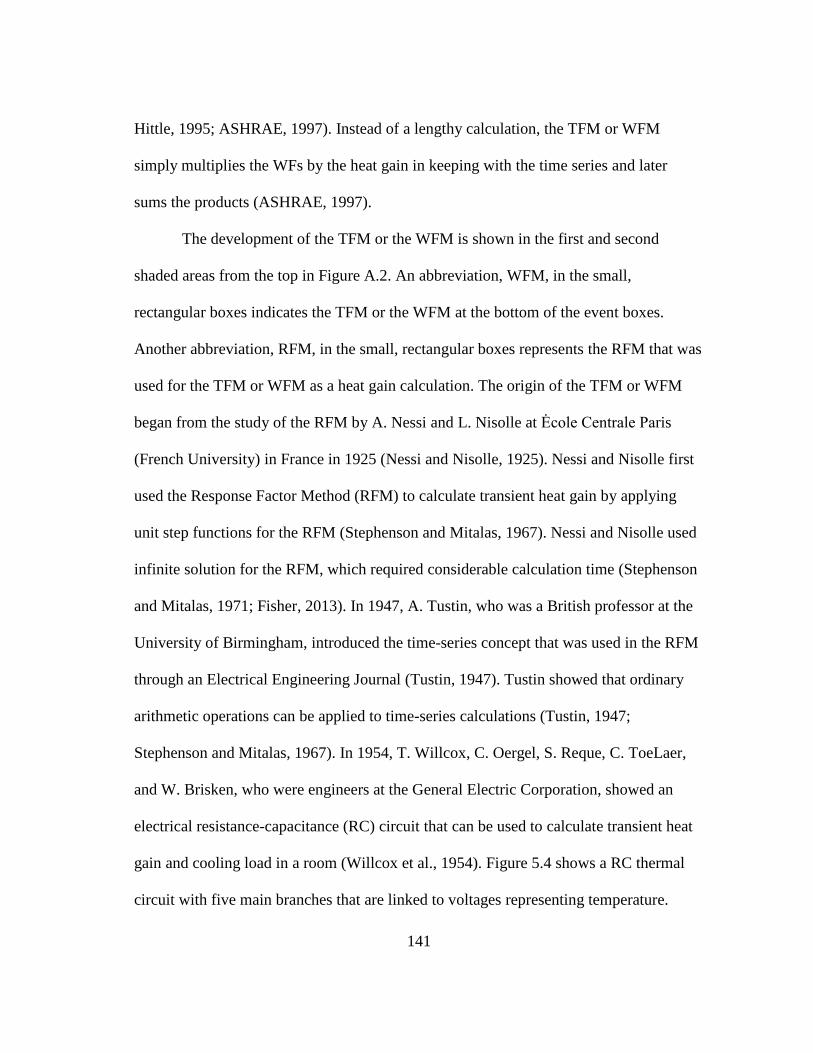
141

Hittle, 1995; ASHRAE, 1997). Instead of a lengthy calculation, the TFM or WFM

simply multiplies the WFs by the heat gain in keeping with the time series and later

sums the products (ASHRAE, 1997).

The development of the TFM or the WFM is shown in the first and second

shaded areas from the top in Figure A.2. An abbreviation, WFM, in the small,

rectangular boxes indicates the TFM or the WFM at the bottom of the event boxes.

Another abbreviation, RFM, in the small, rectangular boxes represents the RFM that was

used for the TFM or WFM as a heat gain calculation. The origin of the TFM or WFM

began from the study of the RFM by A. Nessi and L. Nisolle at Ėcole Centrale Paris

(French University) in France in 1925 (Nessi and Nisolle, 1925). Nessi and Nisolle first

used the Response Factor Method (RFM) to calculate transient heat gain by applying

unit step functions for the RFM (Stephenson and Mitalas, 1967). Nessi and Nisolle used

infinite solution for the RFM, which required considerable calculation time (Stephenson

and Mitalas, 1971; Fisher, 2013). In 1947, A. Tustin, who was a British professor at the

University of Birmingham, introduced the time-series concept that was used in the RFM

through an Electrical Engineering Journal (Tustin, 1947). Tustin showed that ordinary

arithmetic operations can be applied to time-series calculations (Tustin, 1947;

Stephenson and Mitalas, 1967). In 1954, T. Willcox, C. Oergel, S. Reque, C. ToeLaer,

and W. Brisken, who were engineers at the General Electric Corporation, showed an

electrical resistance-capacitance (RC) circuit that can be used to calculate transient heat

gain and cooling load in a room (Willcox et al., 1954). Figure 5.4 shows a RC thermal

circuit with five main branches that are linked to voltages representing temperature.

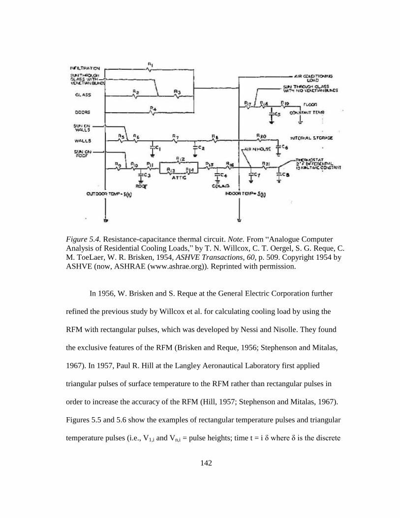
142

Figure 5.4. Resistance-capacitance thermal circuit. Note. From “Analogue Computer

Analysis of Residential Cooling Loads,” by T. N. Willcox, C. T. Oergel, S. G. Reque, C.

M. ToeLaer, W. R. Brisken, 1954, ASHVE Transactions, 60, p. 509. Copyright 1954 by

ASHVE (now, ASHRAE (www.ashrae.org)). Reprinted with permission.

In 1956, W. Brisken and S. Reque at the General Electric Corporation further

refined the previous study by Willcox et al. for calculating cooling load by using the

RFM with rectangular pulses, which was developed by Nessi and Nisolle. They found

the exclusive features of the RFM (Brisken and Reque, 1956; Stephenson and Mitalas,

1967). In 1957, Paul R. Hill at the Langley Aeronautical Laboratory first applied

triangular pulses of surface temperature to the RFM rather than rectangular pulses in

order to increase the accuracy of the RFM (Hill, 1957; Stephenson and Mitalas, 1967).

Figures 5.5 and 5.6 show the examples of rectangular temperature pulses and triangular

temperature pulses (i.e., V1,i and Vn,i = pulse heights; time t = i δ where δ is the discrete

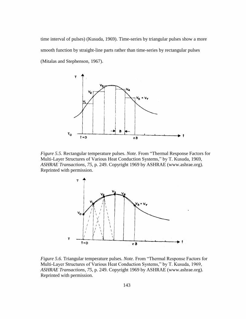
143

time interval of pulses) (Kusuda, 1969). Time-series by triangular pulses show a more

smooth function by straight-line parts rather than time-series by rectangular pulses

(Mitalas and Stephenson, 1967).

Figure 5.5. Rectangular temperature pulses. Note. From “Thermal Response Factors for

Multi-Layer Structures of Various Heat Conduction Systems,” by T. Kusuda, 1969,

ASHRAE Transactions, 75, p. 249. Copyright 1969 by ASHRAE (www.ashrae.org).

Reprinted with permission.

Figure 5.6. Triangular temperature pulses. Note. From “Thermal Response Factors for

Multi-Layer Structures of Various Heat Conduction Systems,” by T. Kusuda, 1969,

ASHRAE Transactions, 75, p. 249. Copyright 1969 by ASHRAE (www.ashrae.org).

Reprinted with permission.

144

In 1965, G. Mitalas at the National Research Council (NRC) Canada proved that

linear mathematical models could be applicable for estimating the thermal behavior in

air conditioned rooms (Mitalas, 1965). This study was important because engineers can

only use the RFM and the WFM when systems can be expressed by linear equations

(Stephenson and Mitalas, 1967).

In 1967, G. Mitalas and D. Stephenson at the NRC Canada developed a new

RFM that used P. Hill’s triangular pulses for digital computers that applied the RFM for

the transient thermal analysis of buildings. G. Mitalas and D. Stephenson’s method

provided a more accurate analysis than W. Brisken and S. Reque’s method that used an

analog model of lumped resistances and capacitances (RC) and rectangular pulses

(Brisken and Reque, 1956; Mitalas and Stephenson, 1967; Kusuda, 1969). The most

important difference is that Mitalas and Stephenson’s method can separately estimate

convection and radiation rather than combined convection and radiation in a room

(Mitalas and Stephenson, 1967). In the same year, a related paper of D. Stephenson and

G. Mitalas introduced the application of the RFM for estimating cooling load and

surface temperature (i.e., the WFM) (Stephenson and Mitalas, 1967).

Also, in 1967, G. Mitalas and J. Arseneault created a FORTRAN IV program for

an IBM-360 computer to calculate RFs for multi-layer walls or roofs. In their program,

the heat flux of the multi-layer systems was able to be calculated numerically by

inverting a matrix of Laplace transforms, which was introduced by L. A. Pipes in 1957

(Pipes, 1957), with the help of the digital computer when triangular pulses were used to

145

simulate the temperature profile of the transient boundary condition (Mitalas and

Arseneault, 1967; Kusuda, 1969). This Laplace transform approach was able to improve

the calculation accuracy by the lumped RC approach of Brisken and Reque. (Kusuda,

1969).

In 1969, T. Kusuda utilized G. Mitalas and J. Arseneaults’ method to calculate

the RFs for analyzing curved exterior surfaces such as cylindrical, spherical buildings,

underground pipes, tunnels, and storage tanks (Kusuda, 1969). In 1971, D. Stephenson

and G. Mitalas further developed the RFM using CTFs (i.e., finite approach) that was

more efficient than the previous RFM regarding speed and memory space of digital

computers (Stephenson and Mitalas, 1971; Fisher, 2013).

Finally, in 1971, the RFM using CTFs was adopted by the ASHRAE Task Group

on Energy Requirements (TGER) (Lokmanhekim ed., 1971). The ASHRAE TGER

recommended the RFM using CTFs and further developed from the RFM to the WFM

using another transfer functions (Lokmanhekim ed., 1971; Kusuda, 1985). The RFM

could be used to calculate time-varying heat gain using wall RFs and surface

temperatures, and the WFM could be used to calculate time-varying cooling load using

WFs and heat gain (Lokmanhekim ed., 1971). In the 1970s, engineers preferred the

WFM over the more time consuming HBM because the speed and memory of digital

computers was limited at the time. (Kusuda, 1985). In 1988, a new method for deciding

146

CTFs11

and WFs was suggested through ASHRAE research projects (Harris and

McQuistion, 1988; Sowell 1988a, 1988b, 1988c; Spitler and Fisher, 1999).

The original WFs developed in 1967 and 1971, called the pre-calculated WFs,

were pre-calculated for typical rooms such as light, medium, and heavy weight

constructions to be used to calculate hourly cooling load. The ASHRAE Handbook of

Fundamentals contained the pre-calculated WFs in the table (Sowell and Hittle, 1995).

The use of pre-calculated WFs reduced the calculation time with a modest loss in

rigorousness of the HBM. In 1979, the deficiency of the pre-calculated WFs was

improved by Z. Cumali, A. Sezgen, and R. Sullivan at the CCB (Cumali et al., 1979).

The new WFs, called the custom WFs, used the actual description data of rooms for

calculating cooling load. The algorithms of the custom WFM were included in the

whole-building energy simulation program, DOE-2.1 (Kerrisk, 1981; Kerrisk et al.,

1981). In the DOE-2.1 program, the custom WFs were generated for time-varying

cooling load in each zone (Kerrisk, 1981; Cumali, 2012). The custom WFs consist of

heat gain WFs and air temperature WFs. Heat gain WFs are the transfer functions for

converting transient heat gains to space cooling load. Air temperature WFs are WFs that

are used to calculate the heat extraction rate and air temperature from the net energy load

including the cooling load of rooms (ASHRAE, 2009). While the pre-calculated WFs

showed some inaccuracy regarding heaving constructed rooms (i.e., lots of thermal mass)

11 CTFs procedure, which was described by H. T. Ceylan and G. E. Myers in 1980, John E. Seem in 1987,

and Kunze Ouyang and Fariborz Haghighat in 1991, was used for the Heat Balance Method (HBM) of

EnergyPlus (Ceylan and Myers, 1980; Seem, 1987; Ouyang and Haghighat, 1991; UIUC and LBNL,

2012).

147

and rooms affected by a large amount of solar load, the custom WFs showed an

improved accuracy for heaving constructed rooms, solar load driven rooms, and even

direct gain passive solar rooms (Schnurr et al., 1979; Kerrisk et al., 1980; Kerrisk, 1981).

In 2012, Z. Cumali proposed improved algorithms based on the custom WFM, which

used a numerical Green’s functions (NGFs) solution, to improve the speed of the time-

varying load calculations in EnergyPlus (Cumali, 2012).

The TFM or WFM explained in this section is currently used for DOE-2.1e,

eQUEST/DOE-2.2, TRACE, and HAP which will be described in Section 5.3.1.2

through 5.3.1.5.

5.2.1.3 Cooling load temperature difference (CLTD)/solar cooling load (SCL)/cooling

load factor (CLF) method

The CLTD/SCL/CLF method is based on the TFM to calculate the cooling load.

This method is a hand calculation with a one-step procedure that does not require the

two steps (i.e., the heat gain and cooling load steps such as the TETD/TA method and

the TFM or the WFM) (ASHRAE, 1997). The CLTD is used to calculate the conductive

cooling loads of walls, roofs, and windows. The Solar Cooling Load (SCL) is used to

determine solar radiation cooling load, and CLF is used to calculate internal cooling load

of lights, peoples, appliances and equipment (McQuiston and Spitler, 1992).

The CLTD/CLF method was developed by William Rudoy and Fernando Duran

at the University of Pittsburg in 1975 (Rudoy and Duran, 1975). This method simplified

the TETD/TA and TFM methods by removing the step that converts radiant heat gain to

cooling load (ASHRAE, 2001). In 1993, this method was modified to become the

148

CLTD/SCL/CLF method by J. D. Spitler, F. C. McQuiston, and K. I. Lindsey as

ASHRAE Research Project-626 (Spitler et al., 1993). The concept of the Solar Cooling

Load (SCL) replaced the CLF for calculating solar radiation cooling load through

fenestration. The SCL reduced the unnecessary step of the CLF and enhanced the

accuracy for estimating the solar radiation load (McQuiston and Spitler, 1992; Spitler et

al., 1993). In addition, the new CLTD/SCL/CLF method improved the effects of zone

response due to zone types using the new WFs and CTFs developed by ASHRAE

Research Project-472 in 1988 (Spitler et al., 1993). Before ASHRAE Research Project-

472, ASHRAE Research Project-359 conducted in 1984 discovered the effects of the

zone response (Sowell and Chiles, 1985).

In the genealogy chart, the original CLTD/CLF method and the new

CLTD/SCL/CLF method are shown in the big rounded boxes. The TRACE program

uses the CLTD/CLF method to size cooling loads.

5.2.1.4 Heat balance method (HBM)

The HBM , also called the thermal balance method, is the scientifically strictest

method to calculate building cooling loads when compared to the TETD/TA method, the

TFM or WFM, and the CLTD/CLF method. The heat balance model has five major

assumptions: constant air temperature in a zone, constant surface temperatures, constant

long and shortwave irradiation, diffuse radiating surfaces, and one-dimensional heat

conduction at the surfaces of the room. In conjunction with these assumptions, the four

processes of the heat balance were analyzed: outside surface heat balance, wall

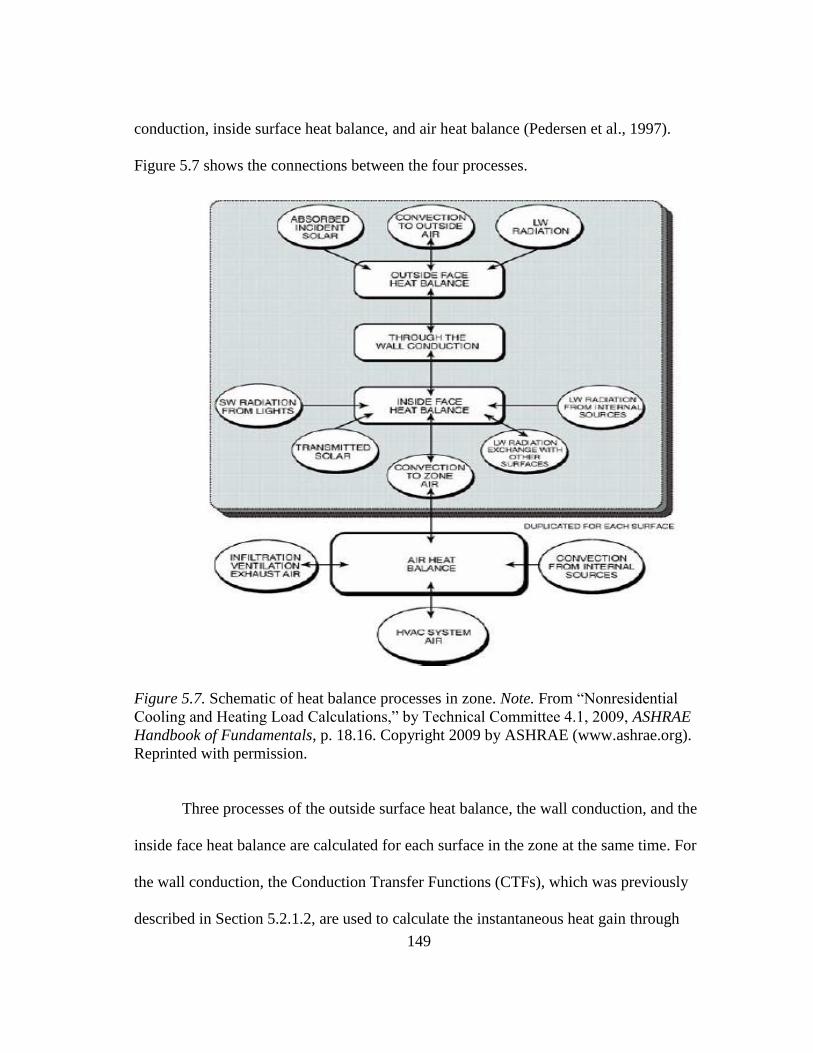
149

conduction, inside surface heat balance, and air heat balance (Pedersen et al., 1997).

Figure 5.7 shows the connections between the four processes.

Figure 5.7. Schematic of heat balance processes in zone. Note. From “Nonresidential

Cooling and Heating Load Calculations,” by Technical Committee 4.1, 2009, ASHRAE

Handbook of Fundamentals, p. 18.16. Copyright 2009 by ASHRAE (www.ashrae.org).

Reprinted with permission.

Three processes of the outside surface heat balance, the wall conduction, and the

inside face heat balance are calculated for each surface in the zone at the same time. For

the wall conduction, the Conduction Transfer Functions (CTFs), which was previously

described in Section 5.2.1.2, are used to calculate the instantaneous heat gain through

150

walls. The air heat balance procedure interacts with the heat convection to zone air

obtained from the three processes for each surface in the zone. The cooling load is

provided by the air heat balance procedure (ASHRAE, 2009).

The advantages of the HBM are that it does not require the simplifying

assumptions of the linear superposition that were used for the WFM or TFM, and the

HBM can analyze changing parameters such as heat convection coefficients at the

surfaces in the zone and transient solar variables that reach into the zone or room

(Sowell and Hittle, 1995). Above all, the procedures in the HBM do not hide the

fundamental processes for accurately calculating each step without risky errors

(Pedersen et al., 1997).

The development of the HBM is shown in the first shaded area from the top in

Figure A.2. An abbreviation, HBM, in the small, rectangular boxes indicates the HBM at

the bottom of the event boxes. The original fundamentals of the HBM were established

by N. Carnot, R. Clausius, and E. F. Obert. One of the fundamentals of the HBM was the

first law of thermodynamics, developed by Clausius in 1851. This principle was based

on Carnot’s study about cycles relating heat and work (Donaldson et al., 1994; Pedersen,

2009). Clausius divided the cycles into minute parts and additionally proposed internal

energy. Inexact differentials were used for heat and work, and an exact differential was

used for energy in the first law. In 1960, this concept was modified by Obert. He

developed a new concept for the first law by introducing time as the independent

variable. Thus, in the first law of Obert, heat and work were also considered as exact

differentials. In other words, Obert defined the first law based on time of the

151

independent variable (Obert, 1960; Pedersen, 2009). Aerospace and other types of

engineers have widely used general heat balance models in their research (Sowell and

Hittle, 1995). The first application for buildings that used a complete method form of the

HBM was developed by Kusuda for the National Bureau of Standards Load

Determination (NBSLD) program (Kusuda, 1976; Sowell and Hittle, 1995; Pedersen et

al., 1997). Kusuda studied the thermal network approach proposed by Buchberg in 1958

to improve the HBM (Kusuda, 1999). The ASHRAE Task Group on Energy

Requirements (TGER) outlined the heat balance algorithm for computer programs in

1975 (ASHRAE, 1975a). Following the development of the NBSLD, in 1977 and 1983,

BLAST12

and TARP13

also employed the HBM. Finally, in 1997, ASHRAE Research

Project-875, sponsored by Technical Committee 4.1, organized the current HBM for the

cooling load calculation and procedure (Pedersen et al., 1997). In the HBM, an improved

CTFs procedure, which was described by H. T. Ceylan and G. E. Myers in 1980, John E.

Seem in 1987, and Kunze Ouyang and Fariborz Haghighat in 1991, was used to

calculate dynamic heat gain through walls and roofs (Ceylan and Myers, 1980; Seem,

1987; Ouyang and Haghighat, 1991; UIUC and LBNL, 2012). The origins of the CTFs

were described in Section 5.2.1.2. The HBM14

was used for calculating cooling load in

12 In 1977, the U.S. Army Construction Engineering Research Laboratory (CERL) developed the Building

Load Analysis and System Thermodynamics (BLAST) program using the modifications of CERL’s first

simulation program (i.e., TASS) and new program code. 13

In 1983, National Bureau of Standards (NBS, now NIST) developed Thermal Analysis Research

Program (TARP) using the heat balance algorithms proposed by ASHRAE in 1975. 14

The HBM calculates heat gain and cooling load at the same time (i.e., no break), whereas the TFM and

the RTS method have a break between heat gain and cooling load calculation (Fisher, 2013).

152

EnergyPlus, the whole-building energy simulation program, released in 2001 (Crawley

et al., 2002).

5.2.1.5 Radiant time series (RTS) method

The RTS method is directly simplified from the HBM and is therefore more

rigorous than other simplified (i.e., non-heat-balance based methods) cooling load

calculations (i.e., the TETD/TA method, the TFM or WFM, and the CLTD/SCL/CLF

method). The RTS method does not need iterative calculations such as the TFM or WFM.

Also, engineers can easily inspect the coefficients of the radiant time series (i.e., the

radiant time factors) for various zone types (Spitler et al., 1997).

The RTS method consists of two series of calculations, as is case for the TFM or

WFM and the TETD/TA method. The first is to calculate time-varying heat gain and the

second is to calculate cooling load using the heat gain. The RTS method uses conduction

time series (CTS) for calculating time-varying heat gain through walls and roofs and

radiant time factors (i.e., the RTS coefficients) for calculating the radiant part of the

cooling load. The convective part of the cooling load that does not require the radiant

time factors (RTFs) is later combined with the radiant part of the cooling load to

generate the total cooling load for a particular hour (ASHRAE, 2009).

The development of the RTS method is shown in the first shaded area from the

top in the 1991-2000 section and the 2001-2010 section of Figure A.2. An abbreviation,

RTS, in the small, rectangular boxes indicates the RTS method at the bottom of the event

boxes. In 1997, Jeffrey D. Spitler, Daniel E. Fisher, and Curtis O. Pedersen proposed the

RTS method as the part of the ASHRAE Research Project-875 (Spitler et al., 1997). In

153

2001, the ASHRAE Fundamentals Handbook adopted the RTS method with the HBM

instead of the TETD/TA method, the TFM or WFM, and the CLTD/SCL/CLF method

(ASHRAE, 2001). As mentioned above in this section, the RTS method uses CTS and

RTFs for calculating each heat gain and cooling load. The origins of CTS started from

the development of response factors (RFs) and conduction transfer functions (CTFs).

The origins of RFs and CTFs were described in Section 5.2.1.2. The RFs were changed

to periodic response factors (PRFs) in the RTS method. PRFs are a simplified version of

response factors, which use a set of 24, for a steady periodic input (Spitler et al., 1997).

In 1999, Spitler and Fisher showed the PRFs can be generated from CTFs using the

assumptions of steady periodic heat input conditions (Spitler and Fisher, 1999). Finally,

the CTS were formed from the further simplification of the 24 periodic response factors,

divided by the overall U factor of walls or roofs (ASHRAE, 2001).

In 1997, the RTFs for calculating the radiant cooling load were described by J.

Spitler, D. Fisher, and C. Pedersen (Spitler et al., 1997). The RTFs was directly

generated by the HBM as the purpose of the RTS method that was to offer the simplified

method from the HBM (ASHRAE, 2001). In 1998, Pedersen et al. developed a computer

program based on the HBM, called Hbfort, to generate the RTFs (Pedersen et al., 1998).

The approach for creating RTFs is similar to the approach for generating the custom

weighting factors using the DOE-2.1 program (ASHRAE, 2001).

5.2.2 The analysis methods of solar system analysis simulation or design

Solar energy analysis programs evaluate the performance of solar systems that

are designed to collect and use solar radiation for thermal or electricity conversion.

154

These programs are used for simulations and design methods: Computer simulations

estimate the time-dependent short-term and long-term performance of solar energy

systems in detail, and design methods analyze the long-term average performance of

solar energy systems with less calculation work than simulations (Klein, 1993). Design

methods are useful for engineers to choose and size solar systems when input data and

solar irradiation have high uncertainty (Evans et al., 1982).

In this study, the solar design methods were mainly investigated. The analysis

methods for detailed solar simulation programs are described in Section 5.2.2.1, and the

design methods for solar design programs (i.e., simplified programs) are explained from

Section 5.2.2.2 to 5.2.2.4. The development of the analysis methods and the design

methods for solar energy programs is shown in the third shaded area from the top in the

pre-1950 section to the 1981-1990 section of Figure A.2 in Appendix A. In Figure A.2,

the abbreviations explained by Figure A.1 in the small, rectangular boxes indicate the

analysis method represented in the event box.

5.2.2.1 The analysis method of detailed simulation programs

In 1972, due to a national direction toward solar energy employment, the first

solar energy simulation programs under U.S. government funding were developed with

the sponsorship of the National Science Foundation (NSF) and the U.S. Energy Research

and Development Administration (ERDA, now the U. S. Department of Energy (US

DOE)). The simulation programs included TRNSYS developed by the University of

Wisconsin-Madison and several programs by the Los Alamos Scientific Laboratory

(LASL, now Los Alamos National Laboratory (LANL)) (Kusuda, 1985; Beckman,

155

1993). In 1975, the TRNSYS program, which was initially developed as a public domain

program, was first publically released by the Solar Energy Laboratory (SEL) at the

University of Wisconsin. The LASL programs were not fully documented and were used

as research tools (Beckman 1993). One of the LASL programs was PASOLE, which

stands for PAssive SOLar Energy. The PASOLE program was used for developing the

Solar Load Ratio (SLR) method, a design method, for passive solar heating applications

(McFarland, 1978; Feldman and Merriam, 1979).

These simulation programs for solar energy applications used a thermal network

approach to solve the time-varying heat transfer problem. This is because the analysis of

a solar heating system on a building requires both an analysis of the time-varying

conditions of the house and the time-dependent solar radiation being collected by the

solar system, including the heat storage effect (Kusuda, 1985). Also, the use of thermal

networks had been shown to be useful in accounting for transient time variation or

temperature dependent values (Niles, 1992). However, the thermal network approach

had limitations for calculating the heat balance in rooms and estimating HVAC systems

used in large-size commercial buildings (Kusuda, 1985).

Before researchers used digital computers to analyze buildings that also have

solar energy systems with the thermal network approach, electrical components were

used in analog circuits because the building thermal components were similar to

electrical circuit components in the thermal network method (Niles, 1992). In 1974,

Peikari explained the electrical network fundamentals (Peikari, 1974). In 1977, Kimura

also discussed the thermal networks for buildings (Kimura, 1977). After the advent of

156

the digital computers, numerical methods were used for thermal network programs to

enhance analysis accuracy. The finite difference method of the numerical approach can

algebraically use the equations to simultaneously or iteratively solve them (Niles, 1992).

In 1979, the PASOLE program, which was introduced by McFarland used the implicit

method of the finite difference method; and in 1983, the SERIRES program (now,

SUNREL), which was developed by Larry Palmiter and Terry Wheeling, used the

explicit method of the finite difference method (McFarland, 1978; Palmiter and

Wheeling, 1983; Niles, 1992).

5.2.2.2 Active solar system design method

Active solar systems consist of solar collectors, storage components, fluid

transport equipment, loads, heat exchangers, auxiliary systems, and other devices

(Duffie, 1993). Domestic water heating systems are typical examples of the active solar

systems. In this study, the development of analysis methods used in the F-Chart

program, which is based on TRNSYS simulation, was summarized and traced.

5.2.2.2.1 Utilizability method

The utilizability method was developed to analyze the incident solar radiation

that reaches the surface of a solar system. The utilizability method was first proposed by

Whillier in 1953 to analyze flat-plate solar collectors (Whillier, 1953a, 1953b). The

method was later extended to estimating concentrating collectors, passive and

photovoltaic systems (Klein, 1993). The solar radiation that reaches a collector can be

expressed in Figure 5.8. Sequence A represents three average days, while sequence B

indicates a clear, an overcast, and an average day. Ic,1 is the critical level which is used to

157

calculate the daily utilizability. Ic,2 would be a higher critical level that might represent a

thermal use with a higher temperature. The utilizable incident solar radiation on the

collectors is indicated as the area above the critical level. The solar radiation area below

the critical level represents the thermal losses of solar collectors, and the area above the

critical level represents the “utilizable” part of the absorbed solar radiation (Klein, 1978;

Klein, 1993).

Figure 5.8. Effect of radiation distribution on the monthly average daily utilizability.

Note. From “Calculation of Flat-Plate Collector Utilizability,” by S. A. Klein, 1978,

Solar Energy, p. 395. Copyright 1978 by Elsevier. Reprinted with permission.

The utilizability method considers the critical insolation level as a constant level.

However, usually most active solar systems have variable critical levels due to the

effects of their thermal storage units and the ambient temperature. Thus, correction

factors for compensating for the errors generated by assuming a constant critical level

were developed, and correlations for the correction factors were obtained by TRNSYS

158

simulation results. The correlation method improved the utilizability method and

enhanced the accuracy of the F-Chart method, which will be explained in the next

section, 5.2.2.2.2.

The development of the utilizability method is shown in the third shaded area

from the top from the pre-1950 section continuing over to the 1981-1990 section of

Figure A.2. An abbreviation, UT, in the small, rectangular boxes indicates the

utilizability method at the bottom of the event boxes. In 1953, Whillier proposed the first

utilizability concept for evaluating flat-plate solar collectors to shorten the calculation

for analyzing the collectors, as part of his Ph.D. dissertation, at the Massachusetts

Institute of Technology (MIT), under Prof. Hottel’s direction (Whillier, 1953b). Before

this study, Hottel and Woertz developed the fundamental equations for flat-plate solar

collectors (Hottel and Woertz, 1942; Hottel, 1950). In 1955, Hottel and Whillier

presented their work (i.e., equations for solar collectors and the utilizability method for

the solar radiation incident) at a conference on the use of solar energy (Hottel and

Whillier, 1955). The equations they used for collectors represented how much useful

solar energy could be collected according to the collector and operating variables. The

variables they used for the collectors are FR(τα) and FRUL (where FR = heat removal

efficiency, τα = suitable mean value of the product of the effective transmittance of the

glass cover plates and the absorptivity of the blackened receiver, UL = overall collector

heat loss coefficient) (Whillier, 1953b). The critical level for determining the utilizable

part of the solar radiation incident on the collectors was defined using the variables for

159

the collectors. Finally, the utilizability ( equation was obtained from a function of the

critical level if the solar radiation data is sufficiently available (Klein, 1993).

In 1963, Liu and Jordan generalized Whillier’s utilizability method (Liu and

Jordan 1963). In Whillier’s utilizability curves, introduced in his dissertation in 1953, he

indicated that the plots of utilizability could be expressed as the calculated utilizability

obtained from the utilizability equation versus the ratio of the critical level to the long-

term average hourly radiation. Whillier also showed utilizability could be determined for

each hour from solar noon because it symmetrically divided the distribution of solar

radiation as shown in Figure 5.8. The limitation of this simplification was that the

utilizability method could not be applied to locations where there was morning fog or

large mountains (i.e., location-dependent utilizability) (Whillier, 1953b; Haberl and Cho,

2004a). Using Whillier’s utilizability curve method, Liu and Jordan’s studies proposed a

cloudiness index in order to create a location-independent utilizability curve method

(Klein, 1993). The cloudiness index depended on the turbidity and cloudiness of an

atmosphere. Liu and Jordan’s study in 1960 proved that the cloudiness index was the

main parameter that affected the sum of the distribution of daily solar radiation upon a

horizontal surface (Liu and Jordan, 1960). Also, Liu and Jordan studied the effects of

collectors that have tilted surfaces using the utilizability curves (Liu and Jordan, 1963).

In 1980 and 1981, Theilacker and Bendt et al. validated Liu and Jordan’s studies with

advanced computers and enough solar radiation data because Liu and Jordan’s studies

were conducted during a period when the capabilities of computers were more limited

and they use insufficient solar radiation data (Theilacker, 1980; Bendt et al., 1981).

160

The disadvantages of Liu and Jordan’s utilizabiliy curves were that there were no

analytical methods to express the utilizability curves, and the utilizability curves were

focused only on surfaces of collectors facing the equator. In 1983, Hollands and Huget

developed an analytical equation for utilizability (Hollands and Huget, 1983). Even

though the algebra of their calculations was complicated, a computerized calculation for

any orientation surfaces was developed from the algebra (Klein and Beckman, 1984). In

the same year, Clark et al. developed a correlation method for utilizability, which was

used for any array orientation (Clark et al., 1983). This computerized method was

algebraically simpler than Hollands and Huget’s method with similar accuracy (Klein

and Beckman, 1984).

In addition to the hourly utilizability method, there was also a daily utilizability

method. While the hourly utilizability represented the utilizable part of the solar

radiation during an hourly period of a specific day, a daily utilizability represented the

average utilizable part of the solar radiation from the sunrise and sunset period for a

month (i.e., this is often called the monthly-average daily utilizability). In other words,

the daily utilizability represented the average solar radiation for each month beyond the

critical level during the period between the rise and fall of sun. In order to use the daily

utilizability concept, the critical level of the solar radiation distribution was considered

as an hourly constant during the entire day. These improved methods for estimating the

daily utilizability were developed even though there was an equation for evaluating the

daily utilizability using the radiation-weighted average of the hourly utilizability values

during all daylight hours (Klein and Beckman, 1984). In 1978, Klein proposed a

161

correlation method for the daily utilizability, where he used curve-fitted values to

develop the daily utilizability correlation and hourly radiation data obtained from Liu

and Jordan’s statistical data, which was given by their study in 1960, instead of using

actual radiation data. Klein’s daily utilizability chart reduced the calculation efforts and

was easily implemented in automated computer programs. The limitation of this method

was that it could be applied to only surfaces headed for the equator (Klein, 1978). In

1979, Collares-Pereira and Rabl developed long-term average energy models using the

daily utilizability correlations to estimate the utilizable solar radiation on flat-pate

collectors, compound parabolic concentrator (CPC), and tracking collectors for east-west,

polar, and two-axis tracking axis. In order to analyze all these collectors, the models

considered the operating temperature used in the solar collectors (Collares-Pereira and

Rabl, 1979).

In 1980, Theilacker proposed a new correlation method that simplified and

improved the accuracy of Klein’s correlation method developed in 1978. This new

method was also applicable to surfaces facing the equator like Klein’s method, but it

added new correlations for surfaces shaded by overhangs and vertical surfaces facing

east and west (Theilacker, 1980; Theilacker and Klein, 1980).

In 1981, Klein et al. developed new tables for vertical surfaces facing south by

using the monthly utilizability obtained from Theilacker’s correlation method (Klein et

al., 1981; Klein and Beckman, 1984). Then, in 1982, Evans et al. developed a new

method that used the actual collector parameters instead of using the critical level. This

method used an empirical approach for the monthly average utilizability to analyze flat-

162

plate collectors, especially for tilted collectors facing south, and the collector efficiency.

This empirical approach could quickly determine the results according to the changes of

location, design and inlet temperature of collectors (Evans et al., 1982).

The utilizability concept explained in this section is currently used for the F-

Chart program developed in 1982, which will be described in Section 5.3.2.1.1.

5.2.2.2.2 F-Chart method

The f-chart method is used to estimate active solar space heating systems and

solar domestic hot water systems. The F-Chart method is a correlation that uses results

from over hundreds of simulation runs using TRNSYS, which is a detailed transient

thermal simulation program, to create the fraction, f (Beckman et al., 1977). The fraction

of the heating load for each month, which will be provided by solar energy, represents f.

The f was developed for defined solar heating systems. The process for gaining the f

values is parallel to the approach of other engineer fields that make correlations of

multiple physical measurements. The f-chart method is usually presented as two

dimensionless variables that are important parameters of solar heating systems (Figure

5.9): The X variable represents the ratio of reference collector energy loss during a

month to total heating load during the same month, and the Y variable represents the

ratio of total energy absorbed on the solar collector during a month to the total heating

load during the same month (Klein, 1993). Figure 5.9 and Figure 5.10 show the

interrelation between f, X, and Y of the solar heating systems using liquid fluids or air

fluids.

163

Figure 5.9. F-chart for liquid systems. Note. From “Chapter 5. Long-Term Performance

of Solar heating Systems,” by W. A. Beckman, S. A. Klein, and J. A. Duffie, 1977, Solar

Heating Design by the F-Chart Method, p. 59. Copyright 1977 by John Wiley & Sons,

Inc. Reprinted with permission.

Figure 5.10. F-chart for air systems. Adapted from “Chapter 5. Long-Term Performance

of Solar heating Systems,” by W. A. Beckman, S. A. Klein, and J. A. Duffie, 1977, Solar

Heating Design by the F-Chart Method, p. 75. Copyright 1977 by John Wiley & Sons,

Inc. Reprinted with permission.

164

In order to gain the fraction of the annual heating load generated from solar

energy, F (i.e., F indicates the annual heating load fraction by solar energy, and f means

the monthly heating load fraction by solar energy), X and Y are obtained for each month.

The value of f, then, is determined by the location of the intersection of the X variable

and Y variable for each month. Finally, the value of F is calculated by a function of f and

the sum of the monthly total (i.e., space and water) heating loads. In the f-chart method,

the fluid flow rate of the collector, the capacity of the thermal storage, and the size of the

load heat exchanger are considered as constant values (Klein, 1993).

The solar energy community used the f-chart method widely in order to design

new systems and analyze the performance of existing systems. However, the f-chart

method has the following disadvantages: a) erroneous results may be produced when the

f-chart method is used for solar systems other than the standard type of systems for

which the f-chart method was initially developed, b) the f-chart method was basically

developed for an ideal system performance estimation and therefore cannot predict the

performance of actual systems that have system characterizations that vary from the

original simulations, c) the f-chart method does not account for small amounts of energy

use required to run controllers, pumps, and fans, and d) ambient solar radiation and

monthly solar radiation are only inputs for the f-chart method in term of the

meteorological information. Therefore, for sites where the input data are not available,

data from nearby sites must be used. The utilizability method, introduced in Section

5.2.2.2.1, more generally accounts for the solar radiation data in detail rather than the f-

chart method (Klein, 1993).

165

The development of the f-chart method is shown in the third shaded area from

the top in the 1971-1980 section of Figure A.2. In 1976, Klein developed the f-chart

method (Klein, 1976; Beckman et al., 1977). The f-chart method was further developed

for customary types of active solar systems such as active domestic hot water systems

(i.e., two-tank domestic water heating systems), pebble bed storage space and domestic

water heating systems, and water storage space and domestic water heating systems.

In 1979, Klein and Beckman developed the monthly utilizability, f-chart method

to extend the f-chart concept to other applications such as concentrating solar collectors

(Klein and Beckman, 1979). To accomplish this, they used the monthly utilizability

concept introduced in the previous section to generalize the f-chart method. In 1981,

Klein and Theilacker proposed a method to estimate radiation data for the tilted surface

of collectors using horizontal solar radiation data because the solar radiation incident on

the collector plane was only for horizontal data (Klein and Theilacker, 1981). In 1983,

Braun et al. expanded the monthly utilizability, f-chart method for close-loop solar

energy systems, developed by Klein and Beckman in 1979, to the monthly utilizability,

f-chart method for open-loop systems (Braun et al., 1983).

Even though the f-chart method was developed to reduce computational effort

compared to the detailed simulation programs, this method still required substantial

computational efforts due to the repetition for the correlation. Thus, various researchers

developed simpler correlation methods that used the results of the f-chart method (Klein,

1993). In 1976, Ward developed a new correlation for solar space heating systems with

water storage that used three collector types (Ward, 1976). In 1978, Barley and Winn

166

proposed a correlation that calculated the annual solar fraction for varying to space and

domestic water heating systems (Barley and Winn, 1978). In the same year, Lameiro and

Bendt proposed a new correlation method, called as the GFL method, for analyzing the

annual solar fraction. In 1980, Wright developed four graphs obtained from the results of

a correlation by the f-chart method in order to further simplify the analysis of actual

solar domestic hot water system performance (Wright, 1980). In 1982, Kreider et al. also

developed a correlation of the annual solar fraction using the f-chart method that was

similar to the previous correlation methods. This correlation method was called as the

W-Chart method (Kreider et al., 1982). These correlation methods, which were based on

the f-chart method, became restrictive because, after the mid-1980s, advanced personal

computers were able to quickly calculate the models of the f-chart method (Klein, 1993).

Other researchers extended the f-chart method because it was initially developed

for only three types of active solar systems as earlier mentioned. In 1979, Jurinak and

Abdel-Khalik performed simulations for air-based solar heating systems using the

TRNSYS program, which led to correlations for air type systems. In their study, a

correction factor obtained from the simulation results was then applied to the f-chart

method for estimating phase change energy storage systems (Jurinak and Abdel-Khalik,

1979). In 1980, Buckles and Klein developed a modified f-chart method to analyze

domestic hot water systems that used for a single tank system. Originally, the f-chart

method was proposed for domestic hot water systems with two tank systems (Buckles

and Klein, 1980). In the same year, Anderson et al. conducted a study concerning

parallel solar heat pump systems. They used the results of simulations to propose a

167

design method for the systems. This design method utilized the f-chart method to

calculate the fraction of the monthly solar energy load (Anderson et al., 1980). In 1985,

Evans et al. performed simulations for active-passive hybrid space heating systems using

the TRNSYS program. Their simulation results developed a new correction factor that

could be applied to the f-chart method for analyzing the hybrid active-passive space

heating systems (Evans et al., 1985).

The F-Chart method explained in this section is currently used for the F-Chart

program developed in 1982, which will be described in Section 5.3.2.1.1.

5.2.2.3 Passive solar system design method

Passive solar systems use solar heating directly (i.e., without pumps, blowers,

etc.) and sometimes include natural passive cooling. Passive solar systems require

simpler and less expensive equipment than that of active solar systems. However,

passive systems for heating need large areas that receive and store solar energy, and the

systems may not be able to effectively store solar energy for long periods (Evans et al.,

1985). In this study, the development of design methods related to the PASOLE program

and the F-Chart program was summarized and traced.

5.2.2.3.1 Solar Load Ratio (SLR) method

The SLR method was developed to use for passive solar systems in a condition

without an active solar system. The SLR method was initially developed for estimating

the required solar collector array size for space heating by Balcomb and Hedstrom in

1976 (Balcomb and Hedstrom, 1976). They correlated the results from a detailed

simulation program, PASOLE, which will be discussed in Section 5.3.2.2.2. This

168

correlation method was divided into a detailed and a simplified type. The detailed

method used the simulation results of system performance for each month, such as the

approach for the development of the f-chart method (Klein, 1993). The SLR was

determined using simulations as the ratio of the solar radiation incident on the collectors

to the building load for each month. After calculating the SLR, the monthly solar

fraction was obtained as a function of the SLR. Also, an annual solar fraction could be

calculated using the load-weighted average of the monthly solar fractions, similar to the

procedure of the f-chart method (Klein, 1993). The simplified method, the SLR method,

used an annual calculation, which used a table that contains the ratio of the heating load

to the collector for annual solar fractions. These tabulated values were obtained from the

results of the detailed hourly simulations using PASOILE (Balcomb and Hedstrom,

1976). However, the SLR method was applicable only for standardized systems (Klein,

1976; Klein 1993).

The development of the SLR method is shown in the third shaded area from the

top in the 1971-1980 section of Figure A.2. An abbreviation, SLR, in the small,

rectangular boxes indicates the SLR method at the bottom of the event boxes. In 1976,

Balcomb and Hedstrom developed the SLR method for estimating the required solar

collector array size for space heating. In 1978, Balcomb and McFarland proposed the

SLR method for passive solar heated walls (Balcomb and McFarland, 1978). In 1981,

Schnurr et al. proposed an extension to the SLR method. This extended method was used

for estimating space and water heating systems used in commercial buildings. In the use

of the results from the DOE-2 detailed simulation program, new correlations were

169

developed for these space and water heating systems (Schnurr et al., 1981). In the same

year, Arney et al. proposed the P-Chart, which is a simplified method of the SLR

method, to optimize passive system size and predict annual solar fraction (Arney et al.,

1981). In 1984 and 1988, Balcomb et al. defined a new SLR method to specifically

analyze passive solar systems (Balcomb et al., 1984; Balcomb and Wray, 1988).

In general, the SLR method was widely received, and tabulated SLR values can

still be seen in popular textbooks such as the Mechanical and Electrical Equipment for

Buildings (Grondzik et al., 2010). However, another new method, called the un-

utilizability method that will be described in the next section, was developed because the

SLR method had limitations.

5.2.2.3.2 Un-utilizability method

The un-utilizability method utilizes the monthly utilizability concept to measure

the solar energy amount that does not reduce ancillary heating load for calculating

heating loads stored in a building structure (i.e., passive solar system) (Monsen and

Klein, 1980; Monsen et al., 1981). The un-utilizability method improved the limitations

of the SLR method, explained in the previous section, in terms of direct gain systems

and collector-storage walls. This is because the SLR method could not account for the

building capacitance effects, interior temperature fluctuation, or alternating room

temperatures, night insulation, and solar absorptance (Monsen et al., 1982).

The development of the un-utilizability method is shown in the third shaded area

from the top in the 1981-1990 section of Figure A.2. An abbreviation, Un-UT, in the

small, rectangular boxes indicates the un-utilizability method at the bottom of the event

170

boxes. The roots of the un-utilizability are the same as those of the utilizability method

for estimating active solar heating systems, which began with the studies of Whillier, Liu

and Jordan, and were then expanded and modified by Klein, and Theilacker and Klein

between 1953 and 1980. These studies were summarized in section 5.2.2.2.1.

In 1980, Monsen and Klein developed the un-utilizability method for passive

solar systems (Monsen and Klein, 1980; Monsen et al., 1981). In this method, they

applied the un-utilizability concept to estimate the performance of direct solar gain

systems. In 1981, Monsen et al. further developed the un-utilizability method to analyze

collector-storage walls (i.e., thermal storage walls). In the same year, Klein et al.

proposed tables for simplifying the un-utilizability procedure (Klein et al., 1981). In

addition, Theilacker et al. extended this method for estimating vertical surfaces with an

overhang, facing south (Theilacker et al., 1981; Jones and Wray, 1992).

The un-utilizability method explained in this section is currently used for the F-

Chart program developed in 1982, which will be described in Section 5.3.2.1.1.

5.2.2.4 Solar photovoltaic (PV) design method

Solar PV, also called solar cells, converts sunlight (i.e., solar radiation) directly

into electricity. The PV F-Chart program (Klein and Beckman, 2001b), which is based

on the utilizability method, the F-Chart method, and Clark et al.’s method (Clark et al.,

1984), can be used to evaluate the monthly performance of PV systems. In this study, the

development of the design method used in the PV F-Chart program is summarized and

traced in the following section.

171

A detailed method provides a short-term (i.e., hourly or less than an hour)

analysis with short-term weather and specific location data, but a simplified method (i.e.,

a design method) achieves a long-term (i.e., monthly average) estimation.

5.2.2.4.1 PV design method

The design method used in the PV F-Chart program also makes use of the

utilizability method, and is generally based on Siegel et al. and Clark et al.’s methods

(Klein and Beckman, 2001b). The detailed origins of the development of the utilizability

method were explained in section 5.2.2.2.1.

The development of the design methods of the PV-F Chart program is shown in

the third shaded area from the top in the 1981-1990 section of Figure A.2. An

abbreviation, PV, in the small, rectangular boxes indicates the PV design method at the

bottom of the event boxes. In 1981, Siegel et al. developed a simplified method to

analyze the monthly-average PV performance. The methods for estimating monthly

average daily PV array output (i.e., electrical output), excess array capacity, and battery

storage were presented in this study. Siegel et al’s method used the TRNSYS compatible

subroutines developed by Evans et al. in 1978 to estimate PV performance data, which

were then compared to the results of the TRNSYS simulations (Evans et al., 1978;

Siegel et al., 1981). Before this study, a method for the long term, monthly average PV

array output was proposed by Evans in 1980 (Evans, 1980). Also, a method for the

excess array capacity was developed by Gupta and Young. Gupta and Young predicted

the excess capacity of the array by using Liu and Jordan’s utilizabilty method developed

in 1963 (Gupta and Young, 1980; Siegel et al., 1981). However, Siegel et al’s method

172

for the excess capacity used Klein’s utilizability method developed in 1978 that used the

monthly average daily utilizability because Klein’s utilizability method had more

computation efficiency than Liu and Jordan’s original utilizability method (Klein, 1978;

Siegel et al., 1981). For estimating the battery charge/discahrge, Siegel et al. used

Shepherd’s battery model proposed in 1965 as well as the model of a 2-V battery cell

explained by Evans et al. in 1978 (Shepherd, 1965; Evans et al., 1978; Siegel et al.,

1981).

In 1984, Clark et al. presented a design method for estimating PV systems to

improve the design methods developed by Evans and Evans et al. in 1980 (Clark et al.,

1984). Evans’s method accounted for the average PV array output without energy

storage capacity using a computational method and graphs. Evans et al.’s method

considered the effect of energy storage capacity for estimating the solar load fraction of

PV systems by using graphs (Evans, 1980; Evans et al., 1980).

In preparation for the coming wide-spread availability of personal computers (i.e.,

microcomputers), Clark et al’s design method presented a proper computational method

by an analytical method for predicting PV systems with or without storage capacity

(Clark et al., 1984). Clark et al.’s method adopted their previous study in 1983 in order

to estimate the PV system performance without battery storage capacity. The previous

study presented the algorithm of the hourly utilizability function rather than the daily

utilizability function used in Siegel et al’s method. The hourly utilizability function

allowed Clark et al.’s method to be used for analyzing hourly loads in the PV systems

(Clark et al., 1983; Clark et al., 1984).

173

The PV design method explained in this section is currently used for the PV F-

Chart program developed in 1983, which will be described in Section 5.3.2.3.1.

5.2.3 The analysis methods of lighting and daylighting analysis simulation

Historically, daylighting analysis programs have used three components in order

to calculate the daylight coming through a window or skylight: the Sky Component

(SC), the External Reflected Component (ERC), and the Internal Reflected Component

(IRC). For this study, the methods for IRC were traced and analyzed. In particular, the

development of the IRC methods used in DAYSIM, Radiance, EnergyPlus, DOE-2, and

Lumen Micro was summarized and traced.

5.2.3.1 Split flux method

The Split flux method is used for calculating the IRC, which is one of the

components of the daylight factor (DF) method (Bryan and Clear, 1980). According to

Bryan and Robert, “… the daylight factor is defined as the ratio between the daylight

illumination at a point in the interior and the simultaneous exterior illumination available

on a horizontal surface from an unobstructed sky (excluding direct sunlight) expressed

as a percentage” (Bryan and Clear, 1980, p.1).

Figure 5.11 shows three paths of light that reach a point on a horizontal work

surface: the sky light (the Sky Component (SC)), the reflected light from external

obstacles (the External Reflected Component (ERC)), and the reflected light from

internal roofs, floors, or walls (the Internal Reflected Component (IRC)). The daylight

factor method accounts for all three components (Bryan and Clear, 1980).

174

Figure 5.11. Components of the daylight factor. Note. From “A Procedure for

Calculating Interior Daylight Illumination with a Programmable Hand Calculator,” by H.

J. Bryan and R. D. Clear, 1980, LBL Report, LBL-11186 C.2, p. 2. Copyright 1980 by

the LBNL.

The split flux method is used to calculate the average IRC, which is the ratio

between the inter-reflected illumination at a point on a horizontal work surface and the

simultaneous sky illumination on an external flat ground. The split flux method uses two

calculations to estimate the IRC: the entering light from the sky and the entering light

from the ground (Bryan and Clear, 1980).

Figure 5.12 indicates the concept of the split flux method:

The light from the sky on entering the room is considered to be modified

by the average reflectance of the floor and those parts of the walls below

the mid-height of the window. The light from the ground is considered to

be modified by the average reflectance of the ceiling and those parts of

the walls above the mid-height of the window. fs = window factor due to

the light incident on the window from sky, Rfw = average reflectance of

the floor and those parts of the walls, below the plane of the mid-height of

the window (excluding the window-wall), fg = window factor due to the

light incident on the window from ground, Rcw = average reflectance of

the ceiling and those parts of the walls, above the plane of the mid-height

of the window (excluding the window-wall) (Bryan and Clear, 1980, p.3)

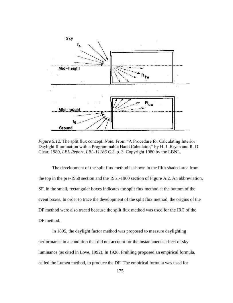
175

Figure 5.12. The split flux concept. Note. From “A Procedure for Calculating Interior

Daylight Illumination with a Programmable Hand Calculator,” by H. J. Bryan and R. D.

Clear, 1980, LBL Report, LBL-11186 C.2, p. 3. Copyright 1980 by the LBNL.

The development of the split flux method is shown in the fifth shaded area from

the top in the pre-1950 section and the 1951-1960 section of Figure A.2. An abbreviation,

SF, in the small, rectangular boxes indicates the split flux method at the bottom of the

event boxes. In order to trace the development of the split flux method, the origins of the

DF method were also traced because the split flux method was used for the IRC of the

DF method.

In 1895, the daylight factor method was proposed to measure daylighting

performance in a condition that did not account for the instantaneous effect of sky

luminance (as cited in Love, 1992). In 1928, Fruhling proposed an empirical formula,

called the Lumen method, to produce the DF. The empirical formula was used for

176

calculating a utilization coefficient, which Fruhling used to create a table of the

utilization factors. Unfortunately, Fruhling’s method did not account for the ERC and

the IRC (as cited in Dresler, 1954). In 1954, Dresler extended Fruhling’s method to

calculate the IRC using the Ulbricht unit sphere principle (Dresler, 1954). About this

same time, Arndt developed a method for calculating the IRC. Arndt’s method adopted a

simpler approach compared to Dresler’s method for calculating the first lighting flux that

reaches an inside surface through a window (as cited in Dresler, 1954).

Finally, also in the same year, Hopkins et al. presented the split flux method

based on Arndt’s method. The split flux method was used to estimate the IRC using an

empirical formula (Hopkinson et al., 1954). The split flux method assumes interior

surfaces of a room are a connected sphere shape and perfectly diffuse with no inner

obstacles, so it works best when a room is shape as a cube and does not have internal

partitions. Due to these reasons, the internally reflected illuminance at the back side of a

room may be over-predicted when the ceiling height of a room is much less than the

depth of the window-wall (Winkelmann and Selkowitz, 1985). In 1989, Tregenza

presented a modified method of the split flux method to account for large external

obstacles such as overhang (Tregenza, 1989).

5.2.3.2 Radiosity method

The radiosity method is an advanced approach used to accurately calculate the

IRC. This procedure uses the energy balance concept for analyzing radiative heat

transfer, which thermal engineers widely use (Goral et al., 1984).

177

Figure 5.13 shows the radiosity method. The term radiosity embodies reflected or

transmitted incident light plus self-emitted light. All the reflection and emission light is

assumed to be ideally diffuse (i.e., Lambertian surfaces or reflectors), and the inner

surface of a room is divided into patches. The reflected light indicates the light leaving a

patch multiplied by the rate of the radiant light leaving a patch which was reached from

the previous patch (i.e., the form-factor (F)) and the reflectivity of a patch. The form-

factor accounts for effect of the geometry. The total reflected and self-emitted light of

each patch is the radiosity of the patch (Greenberg et al., 1986). The radiosity approach

provides a view-independent analysis, which can be used for pre-estimating dynamic

sequences of illumination. In addition, the diffuse reflection as calculated by the

radiosity method can later include surface reflections, which have a small amount of

specular areas with negligible error (Goral et al., 1984).

Figure 5.13. Total radiosity. Note. From “Radiosity: A Method for Computing Global

Illumination,” by D. P. Greenberg, M. F. Cohen, and K. E. Torrance, 1986, The Visual

Computer, 2, p. 292. Copyright 1986 by Springer. Reprinted with permission.

178

Radiosity (B) = the total rate of energy leaving a surface (i.e., sum of emitted

and reflected energy); Emission (E) = The rate of energy (light) emitted from a surface;

Reflectivity (ρ) = the fraction of incident light which is reflected back into the

environment; Form-factor (F) = the fraction of the energy leaving one surface which

lands on another surface; i or j = 1 to N; N = the number of discrete surfaces of

“patches”.

The development of the radiosity method is shown in the fifth shaded area from

the top in the 1971-1980 section and the 1981-1990 section of Figure A.2. An

abbreviation, RS, in the small, rectangular boxes indicates the radiosity method at the

bottom of the event boxes. In In 1966, Sparrow and Cess introduced the radiosity

concept in their book (Sparrow and Cess, 1966). In 1982, Modest utilized the radiosity

method to develop the algorithm for digital computers to calculate the daylighting

effects inside rooms in buildings (Modest, 1982). In 1984, Cindy Goral, Kenneth

Torrance, Donald Greenberg, and Bennett Battaile at Cornell University first used the

radiosity method for computer graphics. At this time, the existing computer graphics did

not use reflection models that considered the reflection effects between diffuse surfaces.

Therefore, the radiosity method, which accounted for reflection s, provided a more

accurate analysis rather than the existing models for the global illumination (Goral et al.,

1984).

The radiosity method was used in the SUPERLITE and DElight programs

(Hitchcock and Carroll, 2003). Version 2.0 of DElight has been integrated into Version

179

1.2 of EnergyPlus, which was released in 2004, as well as the following versions of

EnergyPlus (EERE, n.d.). EnergyPlus will be discussed in Section 5.3.3.2.2.

5.2.3.3 Ray tracing method

Ray tracing is a method of creating computer graphics images with high quality.

The ray tracing method is also used for analyzing inter-reflections between both diffuse

and specular surfaces (Ward et al., 1988). The ray tracing method uses the approach of

tracing the rays of light generated from a source of light to the eye of the viewer

(Kuchkuda, 1988). Figure 5.14 shows the concept of the original ray tracing method.

Figure 5.14. The concept of the ray tracing method. Note. From “COEN 290 Computer

Graphics I,” by B. Grantham, 2008. Reprinted with permission.

In the ray tracing method, the rays of a light source are distributed in all

directions in a room. Among the rays, some rays are reflected and refracted by an object.

Finally, some of these rays reach a viewpoint through an image plane. The idea of the

original ray tracing method was to follow all the paths of the rays from a light source to

180

the viewer. Unfortunately, this approach is wasteful because most of the rays of a light

source do not strike the viewpoint (i.e., image plane) (Kuchkuda, 1988).

Figure 5.15 shows the concept of the improved ray tracing method.

Figure 5.15. The concept of the improved ray tracing method. Note. From “COEN 290

Computer Graphics I,” B. Grantham, 2008. Reprinted with permission.

The improved ray tracing method (i.e., light-backwards ray tracing method)

traces a ray of each point (i.e., each pixel) backwards from the viewer through the image

plane to the object (Arvo, 1986; Kuchkuda, 1988; Ward, 1994). In other words, the paths

of the rays are traced in reversed from a viewpoint to an object in contrast to the original

ray tracing method which followed all of the paths of light.

The development of the improved ray tracing method is shown in the fifth shaded

area from the top in the 1961-1970 section through the 1981-1990 section of Figure A.2.

An abbreviation, RT, in the small, rectangular boxes indicates the ray tracing method at

the bottom of the event boxes. In 1967, Arthur Appel at the IBM Research Center first

proposed the concept of ray tracing (Appel, 1967; Weghorst et al., 1984). In 1971,

Robert A. Goldstein and Roger Nagel at Mathematical Applications Group, Inc. used the

181

ray tracing method to introduce image production software developed by MAGI

(Goldstein and Nagel, 1971; Weghorst et al., 1984). In 1980, Turner Whitted at Bell

Laboratories extended the ray tracing method in order to account for global illumination

in terms of rendering computer graphics images (Whitted, 1980). In 1984, Robert L.

Cook, Thomas Porter, and Loren Carpenter at Lucasfilm Ltd. improved the ray tracing

method by using an analytical function. The unsolved problems of the original ray

tracing method such as motion blur, fuzzy reflections, and depth of field were resolved

by this analytical approach (Cook et al., 1984). In the same year, Hank Weghorst, Gary

Hooper, and Donald Greenberg at Cornell University proposed computational

procedures to reduce the process time for making images by the ray tracing method

(Weghorst et al., 1984). In 1986, James Arvo at Apollo Computer, Inc. described the

backward ray tracing method. The backward ray tracing method provided a solution for

exactly calculating indirect light’s diffuse reflection, which had not been solved (Arvo,

1986).

The advanced ray tracing method (i.e., the backward ray tracing method) has

been used in the Radiance program, developed by Ward in 1988, to analyze the effects

of lighting and daylighting in buildings (Ward et al., 1988; Ward, 1994). The most

recent version of Radiance (i.e., Version 4.2) is currently used (IBPSA USA, 2013).

Radiance will be discussed in Section 5.3.3.1.1.

5.3 Discussion of the Chart for Tracing Specific Programs

In this section, six whole-building energy simulation programs, four solar energy

analysis simulation and design programs, and five lighting and daylighting analysis

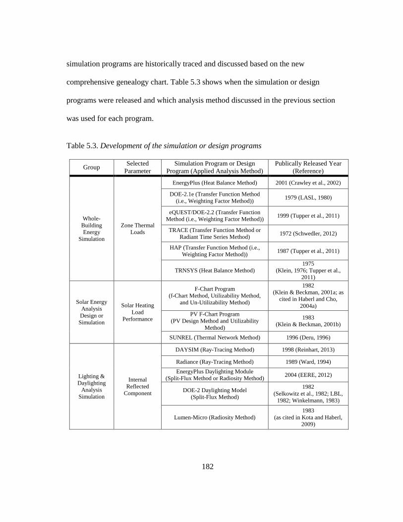
182

simulation programs are historically traced and discussed based on the new

comprehensive genealogy chart. Table 5.3 shows when the simulation or design

programs were released and which analysis method discussed in the previous section

was used for each program.

Table 5.3. Development of the simulation or design programs

Group Selected

Parameter

Simulation Program or Design

Program (Applied Analysis Method)

Publically Released Year

(Reference)

Whole-

Building

Energy

Simulation

Zone Thermal

Loads

EnergyPlus (Heat Balance Method) 2001 (Crawley et al., 2002)

DOE-2.1e (Transfer Function Method

(i.e., Weighting Factor Method)) 1979 (LASL, 1980)

eQUEST/DOE-2.2 (Transfer Function

Method (i.e., Weighting Factor Method)) 1999 (Tupper et al., 2011)

TRACE (Transfer Function Method or

Radiant Time Series Method) 1972 (Schwedler, 2012)

HAP (Transfer Function Method (i.e.,

Weighting Factor Method)) 1987 (Tupper et al., 2011)

TRNSYS (Heat Balance Method)

1975

(Klein, 1976; Tupper et al.,

2011)

Solar Energy

Analysis

Design or

Simulation

Solar Heating

Load

Performance

F-Chart Program

(f-Chart Method, Utilizability Method,

and Un-Utilizability Method)

1982

(Klein & Beckman, 2001a; as

cited in Haberl and Cho,

2004a)

PV F-Chart Program

(PV Design Method and Utilizability

Method)

1983

(Klein & Beckman, 2001b)

SUNREL (Thermal Network Method) 1996 (Deru, 1996)

Lighting &

Daylighting

Analysis

Simulation

Internal

Reflected

Component

DAYSIM (Ray-Tracing Method) 1998 (Reinhart, 2013)

Radiance (Ray-Tracing Method) 1989 (Ward, 1994)

EnergyPlus Daylighting Module

(Split-Flux Method or Radiosity Method) 2004 (EERE, 2012)

DOE-2 Daylighting Model

(Split-Flux Method)

1982

(Selkowitz et al., 1982; LBL,

1982; Winkelmann, 1983)

Lumen-Micro (Radiosity Method)

1983

(as cited in Kota and Haberl,

2009)

183

All the simulation or design programs currently used in the U.S. were released

after 1970 due to the increased availability of powerful computers and improved

compliers. Even though various programs have been developed, some of the programs

have used the same analysis method.

5.3.1 Whole-building energy simulation programs

Whole-building energy simulation programs15

are used to simulate energy use in

buildings, which account for the variation of weather, HVAC system performance, and

occupants in the buildings. Whole-building energy simulation programs are used to

fulfill building energy code or standard compliance, measurement and verification

(M&V), and energy budget conformance as well as determining design phase building

performance, HVAC systems performance, and long-term energy costs (PNNL, 1990;

Higgins, 2012).

5.3.1.1 EnergyPlus

EnergyPlus is the newest whole-building energy simulation program sponsored

by the US DOE. EnergyPlus improved many of the features of previous building

simulation programs, which were discussed in the community of building simulation

specialists (Pedersen et al., 1997). EnergyPlus is a modular structured program that

consists of two basic modules: a heat and mass balance simulation and a building

systems simulation (Crawley et al., 2005). EnergyPlus integrated existing models,

15 This study did not analyze the origins of simulation programs for analyzing the dynamic performace of

mechanical systems in buildings (i.e., BLDSIM, HVACSIM+, and SPARK). BLDSIM was developed by

Shavit in 1978 (as cited in Shavit, 1995). HVACSIM+ and SPARK are component-based simulation

progams like TRNSYS, and they provide improved analysis for HVAC systems in comparison with

whole-building simulation programs (Park et al., 1985; Buhl et al., 1993; Sowell and Hittle, 1995; Wright,

2003).

184

algorithms, or programs in the two modules. The heat and mass balance simulation

module includes the DOE-2 daylighting model (Winkelmann and Selkowitz, 1985) and

DELight2 developed by the Lawrence Berkeley National Laboratory (LBNL), the

window performance analysis of WINDOW developed by the LBNL, and the airflow

network model based on AIRNET developed by Walton at the National Institute of

Standards and Technology (NIST) (Walton, 1989). The building systems simulation

module includes the system and plant models of DOE-2 and BLAST (Pedersen et al.,

1997; UIUC and LBNL, 2012). DOE-2 was released in 1979 by the Lawrence Berkeley

Laboratory (LBL, now LBNL) and the Los Alamos Scientific Laboratory (LASL, now

Los Alamos National Laboratory (LANL) under the U.S. Department of Energy (US

DOE)’s support for the development. The Building Load Analysis and System

Thermodynamics (BLAST) was released in 1977 by the U.S. Army Construction

Engineering Research Laboratory (CERL) under the U.S. Department of Defense (US

DOD)’s support. The development of DOE-2 and BLAST was described in Section

5.1.4.1.

The two modules are managed by the simultaneous solution method based on

IBLAST, which was a research version of BLAST (Crawley et al., 2004; UIUC and

LBNL, 2012).

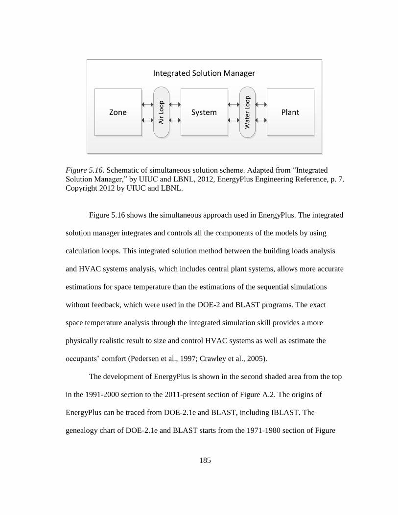
185

Zone System Plant

Integrated Solution Manager

Air

Lo

op

Wat

er L

oo

p

Figure 5.16. Schematic of simultaneous solution scheme. Adapted from “Integrated

Solution Manager,” by UIUC and LBNL, 2012, EnergyPlus Engineering Reference, p. 7.

Copyright 2012 by UIUC and LBNL.

Figure 5.16 shows the simultaneous approach used in EnergyPlus. The integrated

solution manager integrates and controls all the components of the models by using

calculation loops. This integrated solution method between the building loads analysis

and HVAC systems analysis, which includes central plant systems, allows more accurate

estimations for space temperature than the estimations of the sequential simulations

without feedback, which were used in the DOE-2 and BLAST programs. The exact

space temperature analysis through the integrated simulation skill provides a more

physically realistic result to size and control HVAC systems as well as estimate the

occupants’ comfort (Pedersen et al., 1997; Crawley et al., 2005).

The development of EnergyPlus is shown in the second shaded area from the top

in the 1991-2000 section to the 2011-present section of Figure A.2. The origins of

EnergyPlus can be traced from DOE-2.1e and BLAST, including IBLAST. The

genealogy chart of DOE-2.1e and BLAST starts from the 1971-1980 section of Figure

186

A.2., because most of capabilities used in EnergyPlus were obtained from these two

programs. The development of DOE-2.1E will be discussed in the next section.

In terms of the development of BLAST, which is one of the programs that

contributed to EnergyPlus, the National Bureau of Standards Load Determination

(NBSLD) program developed by the National Bureau of Standards (NBS, now the

National Institute of Standards and Technology (NIST)) was an important starting point

to trace BLAST. In 1976, the algorithms used in NBSLD, including the heat balance

method (HBM) or RMTMP (Kusuda and Powell, 1972), were officially released to help

engineers develop their own building simulation programs according to their requests.

The algorithms that came from ASHRAE Task Group on Energy Requirements

(TGER)’s book were corrected and included in the NBSLD algorithms book (Kusuda,

1976). The U.S. Army Construction Engineering Research Laboratory (CERL) used the

NBSLD algorithms to develop CERL’s first building simulation program, called TASS.

In 1977, CERL developed BLAST using the modifications of TASS and a new program

code (Walton, 2001). BLAST was an integrated program including: NBS’s NBSLD (i.e.,

the building load calculation program using HBM), the Computation Consultants Bureau

(CCB)’s total energy plant simulation (TEPS), and CERL’s own system simulation

(Ayres and Stamper, 1995). In 1979 and 1981, BLAST 2.0 and 3.0 were released

(Walton, 2001). In 1994, IBLAST was developed by the University of Illinois at

Urbana-Champaign (UIUC). The HBM concept of BLAST and the simultaneous

solution method of IBLAST significantly impacted the development of EnergyPlus

(Crawley et al., 2005). In the meantime, in 1983, George Walton developed Thermal

187

Analysis Research Program (TARP) at the NIST (Walton, 1983). TARP was derived

from BLAST (Sowell and Hittle, 1995). TARP was able to simultaneously solve heat

balance formulae for multiple rooms in conjunction with air pressure balance formulae.

This unique solution was used for evaluating the movement of natural air, contaminant,

and humidity in multiple rooms (Kusuda, 1985). The one algorithm of the TARP is used

for calculating inside and outside surface convection for EnergyPlus (UIUC and LBNL,

2012).

In 1995, the development of EnergyPlus started because of the need to merge

two simulation programs sponsored by the US DOE and US DOD: DOE-2 and BLAST

(Crawley et al., 1997). In 1997, EnergyPlus was first publically introduced as

EnergyBase (Pedersen et al., 1997). In 1998 and 1999, the alpha and beta version tests

of EnergyPlus were conducted (Crawley et al., 1999). Finally, in 2001, the first version

of EnergyPlus was released (Crawley et al., 2001). In 2003, in Version 1.1, EnergyPlus

incorporated TRNSYS, which will be discussed in Section 5.3.1.6, to calculate PV

systems. From Version 1.2 in 2004, the model, based on the Duffie and Beckman’s

equivalent one-diode model, was used for PV calculations (Duffie and Beckman, 2006;

UIUC and LBNL, 2012). In addition, from Version 1.2, EnergyPlus used DELight 2

developed by LBNL to analyze the effects of lighting and daylighting (UIUC and LBNL,

2012). In 2006, Version 1.3 was released. The existing Airflow Network models (i.e.,

COMIS and ADS) were replaced by a new model with the integrated features from both

models.

188

In 2007, Version 2.0 replaced the existing materials data of DOE-2 and BLAST

with new data from the 2005 ASHRAE Handbook of Fundamentals. In 2008, new

models were added to version 3.0: ventilated slab model, thermal chimney model, and a

cooltower model. In 2009, beginning with version 4.0, users can control the parameters

of window glazing by changing the U factor, solar heat gain coefficient (SHGC), and

visible transmittance (VT) (EERE, n.d.). In 2010, in Version 6.0, the execution time of

EnergyPlus was significantly reduced by approximately 25 to 40% (EERE, 2010). In

2012 and 2013, Versions 7.2 and 8.0 further improved the calculation speed and fixed

previous bugs (EERE, 2012; EERE, 2013b).

5.3.1.2 DOE 2.1e

DOE-2.1e was the main public domain program of the US DOE before

EnergyPlus. Several national laboratories and institutes developed DOE-2.1e to become

a refined and comprehensive simulation program. This program significantly contributed

to the development of the energy saving standards and the design and analysis of

buildings. DOE-2.1e can analyze hourly building loads, energy use, and operating cost.

It can also conduct daylighting analysis, HVAC equipment analysis, and economic

analysis. Currently, DOE-2 based programs are the only programs used to develop code-

compliant simulations certified by the Residential Energy Services Network (RESNET).

Figure 5.17 shows the sequential simulation used in the DOE-2.1e program

without feedback from the previous step. DOE-2.1e consists of four sub-programs:

Loads Analysis, Systems Analysis, Plant Analysis, and Economic Analysis. For the first

step, the Load Analysis sub-program (LOADS) is simulated by using building

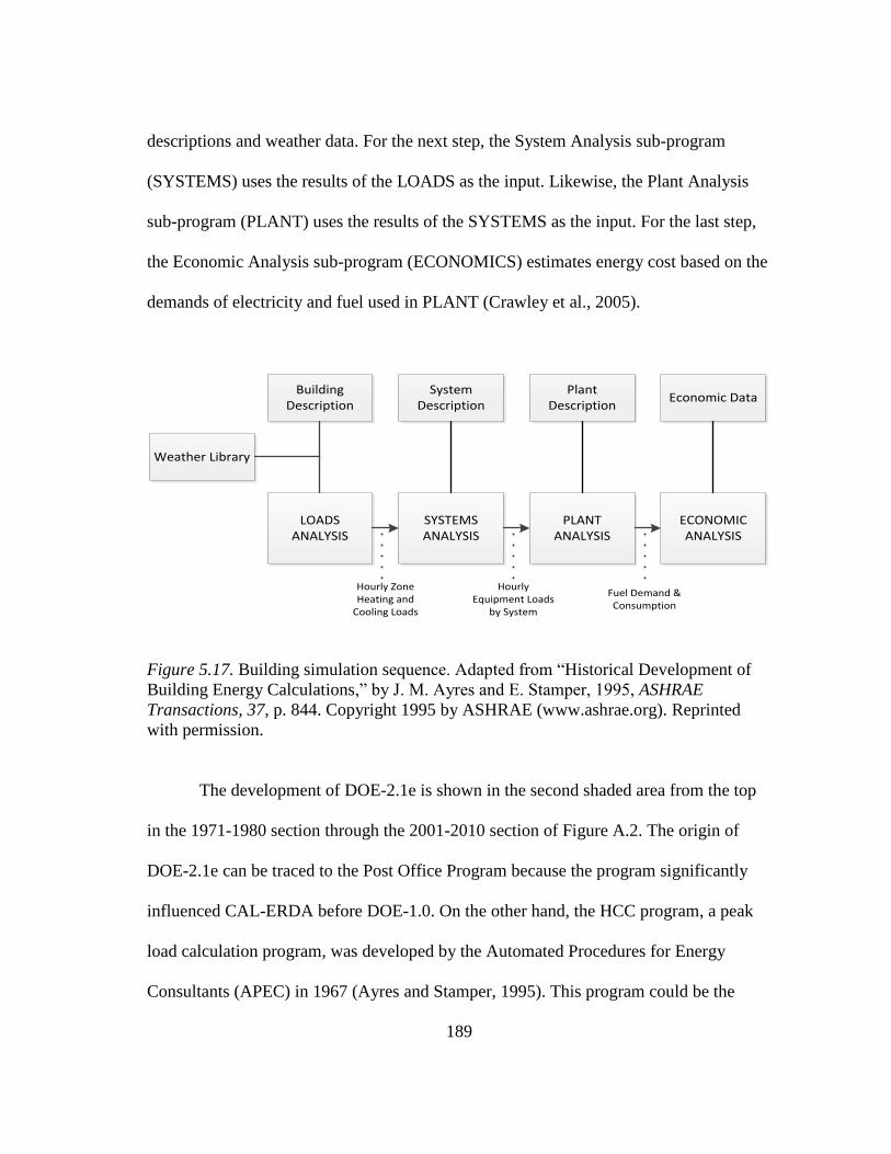
189

descriptions and weather data. For the next step, the System Analysis sub-program

(SYSTEMS) uses the results of the LOADS as the input. Likewise, the Plant Analysis

sub-program (PLANT) uses the results of the SYSTEMS as the input. For the last step,

the Economic Analysis sub-program (ECONOMICS) estimates energy cost based on the

demands of electricity and fuel used in PLANT (Crawley et al., 2005).

SYSTEMS ANALYSIS

LOADS ANALYSIS

PLANT ANALYSIS

ECONOMIC ANALYSIS

Building Description

System Description

Plant Description

Economic Data

Weather Library

Hourly Zone Heating and

Cooling Loads

Hourly Equipment Loads

by System

Fuel Demand & Consumption

Figure 5.17. Building simulation sequence. Adapted from “Historical Development of

Building Energy Calculations,” by J. M. Ayres and E. Stamper, 1995, ASHRAE

Transactions, 37, p. 844. Copyright 1995 by ASHRAE (www.ashrae.org). Reprinted

with permission.

The development of DOE-2.1e is shown in the second shaded area from the top

in the 1971-1980 section through the 2001-2010 section of Figure A.2. The origin of

DOE-2.1e can be traced to the Post Office Program because the program significantly

influenced CAL-ERDA before DOE-1.0. On the other hand, the HCC program, a peak

load calculation program, was developed by the Automated Procedures for Energy

Consultants (APEC) in 1967 (Ayres and Stamper, 1995). This program could be the

190

previous program of the Post Office Program because the load calculation is the

significant part with respect to the development of the whole-building simulation

program even though they do not have a direct connection.

In the late 1960s, the General American Research Division (GARD) of the

General American Transportation Corporation (GATX), which was a subcontractor for

the Post Office facilities division, developed the loads program (i.e., computational

procedures) for the Post Office Program (Stamper 1995; Cumali, 2013). In 1971, the U.S.

post office introduced the post office program (USPS, 1971) to help analyze building

and remodeling efforts for the U.S. Post Office facilities. To accomplish this, the

GARD/GATX engineers developed a building shadow calculation program under the

direction of Metin Lokmanhekim (Kusuda, 1999). The GARD/GATX developed the U.S.

post office program with the ASHRAE TGER report regarding the GARD/GATX

shadow program and the ASHRAE TGER algorithms that used the weighting factor

method (WFM) (USPS, 1971; Kusuda and Powell, 1972; Kusuda, 1999).

In the late 1970s, the Computation Consultants Bureau (CCB) developed the

CAL-ERDA code based on the loads sub-program code used in the Post Office Program.

The name of the CAL-ERDA program was from the name of the sponsors: the

California (CAL) Energy Commission and the United States Energy Research and

Development Administration (ERDA). The code of the Post Office program was a

monolithic and required recompilation for each subroutine. The speed of the CAL-

ERDA was improved by recompiling the code. CCB also developed the Building

Description Language (BDL), which is a user-friendly computer input language (i.e.,

191

familiar terminology), for controlling the load, systems, plant, and economic sub-

programs of the program (Cumali, 2013; Graven and Hirsch, 1977). The Lawrence

Berkeley Laboratory (LBL, now Lawrence Berkeley National Laboratory (LBNL)), The

Argonne Nation Laboratory (ANL), and Los Alamos Scientific Laboratory (LASL, now

Los Alamos National Laboratory (LANL)) also contributed to the development of CAL-

ERDA (Graven and Hirsch, 1977). In 1976, CAL-ERDA was produced. In the same year,

the California Energy Commission (CEC) and ERDA sponsorship for CAL-ERDA

ended and ERDA was integrated into the U.S. Department of Energy (US DOE)

(Birdsall et al., 1990). When Metin Lokmanhekim moved from GARD to LBL, he

brought the skill of the Post Office program to LBL to develop CAL-ERDA (Kusuda,

1999). The LOADS program of CAL-ERDA was developed based on the ASHRAE

algorithms published in 1975. The SYSTEMS program of CAL-ERDA utilized the

equations of the ASHRAE algorithms and the NECAP program (i.e., NASA’s Energy

Cost Analysis Program) for developing the simulation procedure (Graven and Hirsch,

1977).

In 1978, DOE-1, a slightly enhanced version of CAL-ERDA, was released by

CCB, LBL (now LBNL), LASL (now LANL), and ANL (ANL, 1978 as cited in LASL,

1980; Cumali, 2013). The US DOE Office of Buildings and Community Systems

supported the development of DOE-1 (Birdsall et al., 1990). Zulfikar Cumali, Ender

Erdem, Robert Grave, and Metin Lokmanhekim contributed to the development of the

BDL of DOE-1 (LASL, 1980). In 1979 and 1980, DOE-2.0a and DOE-2.1a were

released by LBL and LASL. In the new program, a new BDL had been created for the

192

DOE-2 series to more easily control the LOADS analysis program, the SYSTEMS

program, the PLANT program, and the ECONOMICS analysis program. Frederick Buhl,

James Hirsch, and Mark Roschke designed the BDL of the DOE-2 series. Frederick Buhl

was the principal researcher for the LOADS program, James Hirsh for the SYSTEMS

program, Steven Gates for the PLANT program, Frederick Winkelmann for the

ECONOMICS and LOADS programs, and Mark Roschke for the DOE-2 Solar

Simulator, which was called the Component Based Simulator (CBS) for active solar

systems (LASL, 1980).

In 1982, DOE-2.1b was released by LBL and LANL (LBL, 1982). From this

version, users could use metric inputs for the simulation and could choose metric or

English units for the output result reports. Also, in DOE-2.1b, a simulation method for

daylighting calculation using the split flux method, explained in Section 5.2.3.1, was

installed.

In 1984, DOE-2.1c was released by LBL (LBL, 1984). The funding from the US

DOE had been quickly reduced at ANL and LASL, so LBL became the main national

laboratory for developing new versions of DOE-2 (Ayres and Stamper, 1995). In this

version, algorithms for analyzing sunspaces were added. In 1989, DOE-2.1d was

released by LBL, which included an improved calculation method for diffuse solar

radiation shading (LBL, 1989). In 1993, DOE-2.1e was introduced by LBL and James J.

Hirsch and Associates (JJH). In this version, the models for water loop heat pump

systems, water-cooled condenser option for packaged units, electric and fuel meters,

packaged variable volume temperature (PVVT) system, and gas heat pumps were

193

developed. In 1995, 2000, 2001, 2002, and 2003, DOE-2.1e-Version 087, DOE-2.1e-107,

DOE-2.1e-113, DOE-2.1e-119, and DOE-2.1e-121 were released (LBNL and JJH, 1998;

Haberl and Cho, 2004c; Crawley et al., 2005). DOE-2.1e can be categorized two

versions: the standard DOE-2.1e and the enhanced DOE-2.1e. The standard DOE-2.1e

series, which indicates the versions before Version e-110, were developed by LBNL and

JJH. The enhanced DOE-2.1e series, which means the versions after Version e-110,

were developed by JJH and were improved by fixing existing bugs and having new

features. The features of the enhanced DOE-2.1e contributed to the development of

DOE-2.2 (JJH, 2012).

In 2003, DOE-2.1e-136 was last released as the legacy version (JJH, 2009). In

2005, the development of DOE-2.1e was terminated due to the change of the US DOE’s

funding priorities. The US DOE now focused on developing EnergyPlus, which is

discussed in Section 5.3.1.1. However, the DOE 2.1e based programs such as Visual

DOE and Energygauge developed by each Eley Associates and Florida Solar Energy

Center (FSEC) are currently used (Jacobs and Henderson, 2002; as cited in Tupper et al.,

2011).

5.3.1.3 eQUEST / DOE 2.2

eQUEST or called Quick Energy Simulation Tool is a Graphical User Interface

(GUI) version that uses the DOE-2.2 simulation program. This program is owned by

James J. Hirsch and Associates (JJH) and was first released in 1999 (Jacobs and

Henderson, 2002; as cited in Tupper et al., 2011). DOE 2.2 was developed using the

DOE 2.1e version released in 1994 (LBNL and JJH, 1998). DOE 2.1e has not been

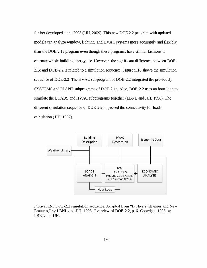
194

further developed since 2003 (JJH, 2009). This new DOE 2.2 program with updated

models can analyze window, lighting, and HVAC systems more accurately and flexibly

than the DOE 2.1e program even though these programs have similar fashions to

estimate whole-building energy use. However, the significant difference between DOE-

2.1e and DOE-2.2 is related to a simulation sequence. Figure 5.18 shows the simulation

sequence of DOE-2.2. The HVAC subprogram of DOE-2.2 integrated the previously

SYSTEMS and PLANT subprograms of DOE-2.1e. Also, DOE-2.2 uses an hour loop to

simulate the LOADS and HVAC subprograms together (LBNL and JJH, 1998). The

different simulation sequence of DOE-2.2 improved the connectivity for loads

calculation (JJH, 1997).

HVAC ANALYSIS

(ref. DOE-2.1e: SYSTEMS and PLANT ANALYSIS)

LOADS ANALYSIS

ECONOMIC ANALYSIS

Building Description

Weather Library

Hour Loop

HVAC Description

Economic Data

Figure 5.18. DOE-2.2 simulation sequence. Adapted from “DOE-2.2 Changes and New

Features,” by LBNL and JJH, 1998, Overview of DOE-2.2, p. 6. Copyright 1998 by

LBNL and JJH.

195

eQUEST based on the DOE-2.2 program is a freeware program, although its

source code is privately owned. It allows users to perform detailed building energy

analysis even though users do not have extensive experience with respect to the DOE-

2.1e simulation program. The user-friendly GUI has a building creation wizard and an

energy efficiency measure (EEM) wizard as well as a graphical module based on DOE-

2.2. Two input options are provided in eQUEST: a wizard option and a detailed input

option. The wizard option works with reduced input data to describe the building such as

building geometry and HVAC systems. The detailed input option allows users to access

and control the full input data of DOE-2.2 (Jacobs and Henderson, 2002).

The development of eQUEST is shown in the second shaded area from the top in

the 1991-2000 section and the 2010-Present section of Figure A.2. The origin of

eQUEST begins DOE 2.1e, which is one of versions of the DOE-2.1 program, developed

in 1993. The DOE 2.1e and DOE-2.1e-087 versions were released by LBL in 1993 and

1995 (LBNL and JJH, 1998; Haberl and Cho, 2004c). Engineers of James J. Hirsch and

Associates (JJH), LBNL (the new name of LBL from 1995), and the Electric Power

Research Institute (EPRI) began to develop DOE-2.2, a new version of DOE-2.1e, in the

early 1990s.

In 1996, PowerDOE, the first GUI program that used DOE-2.2, was created by

JJH along with several partners, under sponsorship by the electric power industry

through EPRI. During the development period for PowerDOE, ownership issues

regarding the DOE-2.2 source code caused a conflict between LBNL and JJH. This

dispute caused LBNL to focus on developing a new whole-building simulation program

196

(i.e., EnergyPlus), which is described in Section 5.3.1.1. During this time, JJH

commercialized and further developed DOE-2.2 using sponsorship from mainly non-

government institutes (i.e., non-US DOE funding) (as cited in Tupper et al., 2011).

In 1999, the eQUEST version 1.0, another GUI program that used DOE 2.2, was

released by JJH. While the development of PowerDOE stopped in 2001 due to funding

difficulty, eQUEST continues to be developed today. In 2000, Version 1.2 of eQUEST

was widely released on the internet. In 2001, Version 2.17c, which included a

refrigeration simulation for grocery stores, was released. In 2007, Version 3.6 was

released and certified for Title 2416

. In 2009, Version 3.63b was released and the US

DOE allowed the version to be the qualified simulation program for the commercial

building tax deductions of the Energy Policy Act of 200517

(EPACT 2005, now the

Emergency Economic Stabilization Act of 2008 (EESA 2008)). In 2010, Version 3.64

was released, which provided a feature to generate the compliance models for LEED

baselines (as cited in Tupper et al., 2011; JJH, 2009). The major funding source (i.e.,

approximately 90%) for the recent eQUEST development was obtained from

California’s Public Goods Charge (PGC), which was an additional charge on electricity

sales (Tupper et al., 2011).

16 The Title 24 code began in 1980 and is the building energy code of the California Energy Commission

(CEC). eQUEST received the qualification for the performance requirement for Title 24 (Tupper et al.,

2011). 17

EPACT 2005 allows the benefit of a tax reduction to building owners who save more than 50% building

energy cost when it compared to the energy cost, meeting ASHRAE Standard 90.1-2001. Energy

simulation programs must be approved by the Internal Revenue Service and US DOE in order to calculate

building energy savings (Tupper et al., 2011).

197

5.3.1.4 TRACE

The Trane Air Conditioning Economics (TRACE) program is a widely used

program among practicing architects and engineers for building loads and energy

calculations. TRACE was developed by the Trane Company. The first version of

TRACE was released in 1972 (as cited in Tupper et al., 2011; Schwedler, 2012).

TRACE has its own calculation engine and Graphical User Interface (GUI). TRACE is

widely used by practicing architects and engineers because the Trane Company strongly

supports TRACE. In 2001, a MS Windows version was developed to simulate hourly

building loads and energy use (Jacobs and Henderson, 2002). TRACE provides users

with several options for calculating cooling loads, including: the Transfer Function

method (TFM) or the Weighting Factor Method (WFM), the Total Equivalent

Temperature Difference / Time Averaging (TETD/TA) method, the Cooling Load

Temperature Difference / Cooling Load Factor (CLTD/CLF) method, and the Radiant

Time Series (RTS) method. These methods were previously discussed in Section 5.2.1.

The development of TRACE is shown in the second shaded area from the top in

the 1971-1980 section to the 2011-Present section of Figure A.2. In 1972, Trane released

the TRACE direct version. TRACE was derived from the Post Office program

developed in 1971 (Sowell and Hittle, 1995). In 1977, the TRACE 77 version was

released, and in 1989, TRACE 600 was released, which was the upgraded version of

TRACE 77 (as cited in Tupper et al., 2011).

The Trane Company released TRACE 700 in 1998, which was the first MS

Windows version of the program (Tupper et al., 2011). Since 2000, engineers and

198

architects have widely used both the TRACE program and the HAP program from the

Carrier company. Both programs are used to calculate building loads, size of HVAC

systems, and annual energy use (Jacobs and Henderson, 2002). TRACE has continued to

be released and updated until now (i.e., TRACE 700 Windows full Version in 2001,

TRACE 700 Version 4.1 in 2002, TRACE 700 Version 6.0 in 2006, TRACE 700

Version 6.2 in 2008, and TRACE 700 Version 6.2.10 in 2013) (Tupper et al., 2011;

Trane, 2013). TRACE 700 Version 6.2 added the RTS method, which was described in

Section 5.2.1.5, to calculate peak cooling loads. The RTS method was not a feature

available in the 600 version.

5.3.1.5 HAP

The Hourly Analysis Program (HAP) was developed by the Carrier Company.

The first version of HAP was released in 1987 (Tupper et al., 2011). HAP has its own

calculation engine and GUI based on the MS Windows platform (Jacobs and Henderson,

2002; EERE, 2011a). Practicing engineers and architects widely use the HAP program

because the Carrier Company strongly supports HAP (Jacobs and Henderson, 2002).

Dynamic heat gain, design peak loads, HVAC system sizing and design, and annual

hourly energy use can be simulated by HAP (EERE, 2011a).

The development of HAP is shown in the second shaded area from the top in the

1981-1990 section through the 2011-Present section of Figure A.2. In 1960, the System

Design Manual of Carrier was published to help engineers learn the HVAC system

design method. This book contained manual calculation procedures for estimating

dynamic heat gain and design peak loads (Carrier, 1960). In 1981, Carrier released the

199

Commercial Load Estimating program Version 1.0, which was a Personal Computer

(PC) based program, for automatically estimating the building design peak loads

(Tupper et al., 2011; Farzad, 2012). The program provided engineers with a time-saving,

cost effective way to calculate the design peak loads. The program was well-received

since engineers were spared the tedious hand calculations needed for calculating the

design peak loads. Shortly after the Commercial Load Estimating program Version 1.0,

the Bin Opcost analysis program Version 1.0 was developed for estimating the annual

energy use in buildings that used ASHRAE’s Bin method (Farzad, 2012).

In 1987, HAP Version 1.0 was released, which was a follow-up program to

Carrier’s Commercial Load Estimating and Bin Opcost analysis programs. HAP Version

1.0 combined the functions of calculating the design peak loads, HVAC system design,

and hourly energy analysis. By 1987, the development of PCs had improved enough that

the accuracy of energy analysis using an hour by hour procedure was possible.

Therefore, in 1989, HAP Version 2.0 was released. This version applied ASHRAE’s

Transfer Function Method (TFM) to calculate building loads (Farzad, 2012; EERE

2012). In 1993 and 1999, Version 3.0 and Version 4.0 were respectively released.

Version 4.0 moved HAP from the MS DOS platform to the MS Windows platform

(Farzad, 2012). Version 4.0 included a MS Windows-based Graphical User Interface

(GUI) to more easily faciliate input data (Farzad, 2012; Carrier, 2013).

HAP has continued to be released and updated until now. In 2002, Version 4.1

added the capabilities to calculate the energy use and cost regarding air-side system and

plant operations. In 2006, Version 4.3 implemented the option for importing gbXML

200

building information format, which is a new data format to connect data between

building design and information programs and building energy simulation programs.

Also, Version 4.3 provided a Building Wizard program to provide useful schematic or

preliminary design options. In 2008, Version 4.4 provided useful options to help users

achieve the LEED Energy and Atmosphere Credit 1. In addition, Version 4.4 updated

new Wizard features, which were based on the Wizard options of Version 4.3, to help

users more quickly enter the needed input data for a simulation. In 2012, Version 4.6

added more new HVAC models such as variable refrigerant flow (VRF) equipment and

condensing and non-condensing boilers, which were based on customer surveys (Carrier,

2013).

HAP currently uses ASHRAE’s Transfer Function Method (TFM) or Weighting

Factor Method (WFM) to calculate dynamic heat gains and building loads, which was

explained Section 5.2.1.2 (Farzad, 2012; EERE 2012).

5.3.1.6 TRNSYS

TRNSYS is a widely used modular or component-based program. Originally, the

program was called TRANsient SYStems (TRANSYS), which was later changed to

TRNSYS because only six letters were permitted in early version of FORTRAN

compilers (Beckman, 1993). This program was developed to simulate solar systems with

the transient variation as the program name indicates. The first publically available

version of TRNSYS was released at the University of Wisconsin-Madison in 1975

(Tupper et al., 2011). This program originally was developed for solar thermal

simulations, but has extended a major contribution to building energy simulation,

201

passive solar, photovoltaic (PV), and even hydrogen production analysis (Athienitis, et

al., 2012).

TRNSYS uses connecting modular subroutines to perform an analysis. The

subroutines (i.e., models) contain mathematical equations (i.e., ordinary differential or

algebraic equations) and all necessary aspects for calculating each system. This

connective solution approach has been shown to be more rigorous and accurate than

other whole-building simulation programs that must estimate solar heating and cooling

systems used in buildings (Kusuda, 1985; Sowell and Hittle, 1995). However, the

solution approach is limited for large-size buildings because large-size buildings

simultaneously have the heating and cooling loads, and high internal loads occur in these

types of buildings. For large-size buildings, the whole-building simulation programs,

which are previously described in Section 5.3.1.1 through 5.3.1.5, are more proper

(ASHRAE, 1981). The algorithms of the whole-building simulation programs were more

detailed for calculating conventional cooling and heating loads (Sowell and Hittle,

1995).

The development of TRNSYS is shown in the second shaded area from the top in

the 1971-1980 section through the 2011-Present section of Figure A.2. In the early

1970s, the Solar Energy Laboratory (SEL) at the University of Wisconsin-Madison

(UWM) started to study solar energy technologies, under the sponsorship of the US

DOE (as cited in Tupper et al., 2011). Sanford Klein, then a graduate student at the

University of Wisconsin-Madison, proposed the methods for accounting for the thermal

storage effect of solar collectors as his MS thesis. He later developed a multi-node

202

collector model for analyzing the transient effect of thermal storage (Klein, 1973). In the

same year, Klein and SEL proposed TRNSYS using Klein’s method for solar collectors

as one of the components of TRNSYS (as cited in Klein, 1976). In 1975, TRNSYS was

publically released, and Klein finished his dissertation in 1976 (Klein, 1976; Tupper et

al., 2011). In 1977, William Beckman, Sanford Klein, and John Duffie completely

described the F-Chart method that was introduced by Klein’s PhD dissertation (Beckman

et al., 1977). The F-Chart method consists of correlations based on thousands of the

simulation results using TRNSYS.

In 1993, the SEL released TRNSYS Version 14.2, which was the first MS

Windows version (Tupper et al., 2011). Unfortunately, the algorithms in TRNSYS

required a lot of computing time to simulate complete system. However, although a

program initially, this problem was resolved as more powerful Personal Computers

(PCs) became available. In the late 1990s, the US DOE decided to stop supporting

TRNSYS and to focus on developing a new whole-building simulation program (i.e.,

EnergyPlus), which is described in Section 5.3.1.1. From that time, the main funding

source for the development of TRNSYS has been reinvestment through the TRNSYS

sales revenue (Tupper et al., 2011).

Since 1975, TRNSYS has been updated and widely used in the U.S. (i.e., Version

15 in 2001, Version 16 in 2004, Version 17 in 2010, and Version 17.1 in 2012).

TRNSYS uses the finite difference and network approach (i.e., the connecting approach

by using models that contain differential equations) to analyze solar heating and cooling

systems used in buildings (Kusuda, 1985). In addition, TRNSYS uses the Conduction

203

Transfer Function (CTF) method explained in Section 5.2.1.2 to analyze transient heat

gain through walls and roofs (SEL, 2010; Delcroix et al, 2012). TRNSYS uses the Heat

Balance Method (HBM) described in Section 5.2.1.4 to estimate cooling loads (SEL,

2010).

5.3.2 Solar analysis simulation or design programs

Solar energy analysis programs evaluate the performance of systems that are

designed to collect and use solar radiation for thermal or electrical conversion. The

programs are used for simulations and design methods (i.e., simplified methods).

Detailed simulation programs estimate the time-dependent short-term and long-term

performance of solar energy systems in detail, and design programs (i.e., simplified

programs) analyze the long-term average performance of solar energy systems with less

calculation work than simulations (Klein, 1993). Detailed simulation programs are used

to create the most accurate results. On the other hand, design programs are used to make

quick results as a design step because an iterative process is required at the design step

(Athienitis, et al., 2012). In addition, design programs are useful for engineers to choose

and size solar systems when input and solar irradiation data has high uncertainty (Evans

et al., 1982).

5.3.2.1 Active solar system analysis

Active solar heating and cooling systems contain unpredictable variables such as

nonlinear reaction parameters of systems with respect to solar radiation, weather data,

and transient variation (Duffie, 1993). In order to simulate solar systems, two types of

simulation programs were developed: the detailed simulation and the design analysis

204

programs. TRNSYS, the detailed simulation program, was explained in Section 5.3.1.6.

In terms of the design analysis program for active solar system analysis, F-Chart

program was selected in this study.

5.3.2.1.1 F-Chart program

The F-Chart program was proposed by SEL at the University of Wisconsin-

Madison. The F-Chart method used in the F-Chart program was first introduced in

Klein’s PhD dissertation (Klein, 1976). The utilizability method and the F-Chart method,

explained in Section 5.2.2.2.1 and 5.2.2.2.2, are used to analyze active solar space

heating systems and solar domestic hot water systems. A correlation using results from

over hundred simulation runs through TRNSYS, which is the detailed transient thermal

simulation program, create the fraction, f (Beckman et al., 1977). The F-Chart program

was originally created in the BASIC platform (i.e., now in the Windows platform). This

computer program reduces tedious work, such as controlling of solar radiation data of

the F-Chart method by utilizing a computer speed. This program also provides economic

analysis such as costs, life cycle, and cash flow of the solar systems (Klein and

Beckman, 2001a; Athienitis, et al., 2012). The F-Chart program uses the F-Chart method

to estimate active domestic hot water system, pebble bed storage space and domestic

water heating systems, water storage space and/or domestic water heating systems, and

building storage systems. The F-Chart program also uses the utilizability, F-Chart

method, explained in Section 5.2.2.2.2 to analyze general solar heating systems. In

addition, the F-Chart program uses the un-utilizability method, explained in Section

205

5.2.2.3.2, to estimate passive direct-gain system and storage wall systems (Klein and

Beckman, 2001a).

The development of the F-Chart program is shown in the fourth shaded area from

the top in the 1981-1990 section through the 2001-2010 section of Figure A.2.

The F-Chart program was first developed for mainframe computers using the

FORTRAN platform. Until 1982, the F-Chart program (i.e., Version 1.0 through 4.1)

had been developed in FORTRAN. From 1983 to1992, the versions of the F-Chart

program (i.e. Version 5.0 series) were written in BASIC for microcomputers. Since

1993, the F-Chart program has been developed in the Windows platform (as cited in

Haberl and Cho, 2004a; Klein and Beckman, 2001a).

5.3.2.2 Passive solar system analysis

Passive solar heating and cooling systems contain unpredictable variables such as

nonlinear reaction parameters of systems with respect to solar radiation, weather data,

and transient variation (Duffie, 1993). In order to simulate passive solar systems, two

types of simulation programs were developed: the detailed simulation and the design

analysis programs. In the following sections, 5.3.2.2.1 and 5.3.2.2.2, the detailed

simulation programs (i.e., SUNREL and PASOLE) were discussed. In terms of the

design analysis program for passive solar system analysis, the F-Chart program was

explained in the previous section, Section 5.3.2.1.1.

5.3.2.2.1 SUNREL

SUNREL is the whole-building simulation program for small-size buildings, but

suitable for the buildings that have passive solar systems (EERE, 2011b). This is because

206

the thermal network method used in SUNREL had limitations for calculating the heat

balance in rooms and estimating HVAC systems used in large-size commercial buildings

(Kusuda, 1985). SUNREL is an upgraded version of SERIRES developed by the Solar

Energy Research Institute (SERI, now called the National Renewable Energy

Laboratory, NREL) in 1983 (Palmiter and Wheeling, 1983). SUNREL can be used to

calculate the effectiveness of different types of passive solar buildings. SUNREL is used

as the building physics and mathematics engine in Targeted Retrofit Energy Analysis

Tool (TREAT), which was developed for single and multifamily building analysis

software (NREL, 2005; EERE, 2011b).

The development of the SUNREL program is shown in the fourth shaded area

from the top in the 1971-1980 section through the 2001-2010 section of Figure A.2. In

1980, SUNCAT Version 2.4 was developed by Larry Palmiter and Terry Wheeling at

Ecotope Group, a non-profit organization for energy research and education (as cited in

Palmiter and Wheeling, 1983). The SUNCAT program was one of a series of programs

developed by Palmiter and Wheeling over four years. In 1983, the SERIRES version 1.0

developed by the same authors under contract to SERI (now NREL). SERIRES stands

for Solar Energy Research Institute Residential Energy Simulator (Palmiter and

Wheeling, 1983). In 1996, SERIRES was upgraded to SUNREL by Colorado State

University and NREL (Deru, 1996). One of the upgrades was to make the format of the

program flexible with respect to future improvements and visual user interfaces, using

the FORTRAN language. SUNREL uses the solar geometry equations by McFarland in

207

1979 and the solar declination equation by Duffie and Beckman in 1991 (Deru, 1996;

Deru et al., 2002).

SUNREL used a thermal network approach to solve the time-varying heat

transfer problem. This is because the analysis of a solar heating system on a building

requires both an analysis of the time-varying conditions of the house as well as the time-

dependent solar radiation being collected by the solar system (Kusuda, 1985). Also, the

use of thermal networks had been shown to be useful in accounting for transient time

variation or temperature dependent values. The SERIRES program, developed by Larry

Palmiter and Terry Wheeling in 1983, used the explicit approach of the finite difference

method (Niles, 1992).

5.3.2.2.2 PASOLE

In 1972, due to the national scheme for solar energy employment, the first solar

energy simulation programs funded by the U.S. government were developed under the

sponsorship of the National Science Foundation (NSF) and the U. S. Energy Research

and Development Administration (ERDA, now the U. S. Department of Energy (US

DOE)) (Kusuda, 1985; Beckman, 1993). One of the Los Alamos Scientific Laboratory

(LASL, now Los Alamos National Laboratory (LANL)) programs is PASOLE, which

stands for PAssive SOLar Energy. PASOLE was introduced by McFarland at LASL in

1978. This simulation program was created to simulate detailed analyses for passive

solar systems. Users were able to manipulate a thermal network model used in PASOLE

by utilizing nodes, connections of nodes, and parameters between nodes and

208

connections. The nodes and parameters were created in FORTRAN subroutines

(McFarland, 1978; Feldman and Merriam, 1979).

The development of the PASOLE program is shown in the fourth shaded area

from the top in the 1971-1980 section of Figure A.2. In 1978, PASOLE was introduced

by R. D. McFarland at the LASL (McFarland, 1978). John Douglas Balcomb proposed

the simulation type idea of creating PASOLE. J. C. Hedstrom developed a one-mass-

node simulation program, which contributed to the development of PASOLE

(McFarland, 1978). The LASL utilized PASOLE to develop passive solar models for

Trombe walls, direct-gain systems, and sunspaces. A correlation using results from over

hundred simulation runs through PASOLE (i.e., the detailed simulation program) created

the Solar Load Ratio (SLR) method (Balcomb, 1992). The SLR method, the design

method for a monthly backup heat analysis, was discussed in Section 5.2.2.3.1.

After the advent of digital computers, numerical methods were used for thermal

network based computer programs to enhance analysis accuracy. The finite difference

method of the numerical approach can algebraically use equations to simultaneously or

iteratively solve the equations. The thermal network approach program, PASOLE, used

the implicit approach of the finite difference method (Niles, 1992).

5.3.2.3 Solar photovoltaic (PV) analysis

PV analysis programs estimate the electrical output of PV systems, including PV

panels, energy inverters, and energy storage. The analysis is based on geometric

locations and weather data (Klise and Stein, 2009). In this study, the PV F-Chart

program that uses a simplified method (i.e., design method) will be discussed. Detailed

209

PV programs (i.e., simulation programs), such as PV-DesignPro developed from Maui

Solar and PVWatt developed from NREL, were not discussed in this study. Most

detailed programs in the U.S. use the PVFORM model (i.e., detailed model) developed

in 1985 at the Sandia National Laboratory (Menicucci, 1985, 1986). Simulation

programs provide a short-term (i.e., hourly or less than an hour) analysis with short-term

weather and specific location data, but the PV F-Chart program achieves a long-term

(i.e., monthly average) estimation of PV systems (Klein and Beckman, 2001b).

5.3.2.3.1 PV F-Chart program

The PV F-Chart program was developed by SEL at the University of Wisconsin

in 1983 (Haberl and Cho, 2004b). This program is used for estimating the long-term PV

system analysis. In addition, this program provides the economic analysis for life cycle

costs. The PV F-Chart program consists of major four algorithms: monthly average PV

array output, monthly average excess energy, effect of load variability, and battery

storage systems. The PV design method, explained in Section 5.2.2.4.1, is largely used

for the four algorithms. In addition, the utilizability method, explained in Section

5.2.2.2.1, is employed for the monthly average excess energy and effect of load

variability algorithms (Klein and Beckman, 2001b). For a plane of array radiation

analysis, a simple isotropic sky model of Liu and Jordan developed in 1963 is used in the

PV-F Chart program (Klise and Stein, 2009).

The development of the PV F-Chart program is shown in the fourth shaded area

from the top in the 1981-1990 section through the 2001-2010 section of Figure A.2. The

PV F-Chart program was first developed for mainframe computers using the FORTRAN

210

platform. Since 1993, the PV F-Chart program has been developed in the Windows

platform (as cited in Haberl and Cho, 2004a; Klein and Beckman, 2001b).

5.3.3 Lighting and daylighting analysis simulation programs

In order to analyze the daylight or natural light effect, several methods were

developed: rules of thumb, graphical methods, and methods of utilizing physical models

(as cited in Ubbelohde and Humann, 1998). Lighting designers wanted to estimate

interior illumination in buildings with one of methods above. Several calculation

methods were developed to accurately analyze the interior light. Many lighting designers

assumed computer simulation programs were able to be used for estimating interior light

with the most accurate approach (Ubbelohde and Humann, 1998).

Daylighting strategies use natural light to reduce the loads of artificial electrical

lighting systems. A proper daylighting design can provide improved illumination for

occupants and can reduce a building’s energy use. Building orientation, window size,

shading (i.e., overhangs and fins), and the use of artificial lighting systems are involved

in a daylighting simulation. Daylighting analysis simulation programs are primarily used

to calculate the lighting levels at specific points in a space. They can also keep track of

how much artificial lighting is needed to supplement the illumination to meet

predetermined lighting levels. The simulation programs for lighting and daylighting

analysis used in this study are the following: Radiance, DAYSIM, and Lumen Micro as

an independent program; the daylighting model in EnergyPlus (i.e., DElight) and the

daylighting routines in DOE-2.1e as an integrated program.

211

5.3.3.1 Independent program

Daylighting analysis programs can be used to estimate building energy use by

daylighting strategies. However, in this independent program section, lighting and

daylighting design or visualization programs are discussed. The independent programs

are not connected to building energy use analysis accounting for electric lighting and

building loads related to HVAC system analysis.

5.3.3.1.1 Radiance

Radiance developed in the UNIX platform is an advanced lighting and

daylighting simulation program for analyzing color (i.e. renderings) and illuminance of

building inside and outside light (EERE, 2011c). Rendered images generated from

Radiance are significantly beneficial to evaluate lighting distribution and aesthetics

(Papamichael et al., 1998). Radiance uses the light-backwards ray tracing method

discussed in Section 5.2.3.2 in order to analyze inter-reflections between both diffuse

and specular surfaces (Ward et al., 1988; Ward, 1994). A Monte Carlo method (i.e., a

numerical method) also was used in Radiance to estimate indirect illuminance (Howell

and Perlmutter, 1964; Ward et al., 1988). Radiance adopted all weather sky model

developed by Perez, Seals, and Michalsky to account for room illuminance under sky

conditions (Kota, 2011).

Radiance is an integrated program with different programs (Papamichael et al.,

1998). For generating sky models, the GENSKY and GENDAYLIT programs are used

in Radiance: A sky scene description of the CIE standard sky distribution is generated by

GENSKY, a sky scene description by using Perez’s all weather sky model is produced

212

by GENDAYLIT (Mardaljevic, 2000). Also, the RAD program helps users manage

input control parameters (Papamichael et al., 1998).

The development of the Radiance program is shown in the sixth shaded area

from the top in the 1981-1990 section through the 2011-Present section of Figure A.2.

Radiance was developed by Gregory Ward at the LBL and the Ecole Polytechnique

Federal de Lausanne (EPFL, Swiss institute). The development of this program was

initiated by studying ray tracing algorithms discussed in Section 5.2.3.2. US DOE and

later the Swiss federal government decided to support this study after they found energy

saving opportunities through lighting and daylighting strategies. In 1989, Radiance was

first released (Ward, 1994). In 1990, Version 1.2 and 1.3 were released. Luminaire data

of the Illuminating Engineering Society (IES) format was added to Version 1.3 using

conversion utility. In 1991, Version 2.0 was released. An option for estimating

irradiance in lieu of radiance was added to this Version 2.0. In 1992, 1993, 1994, and

1995, Version 2.1, Version 2.3, Version, 2.4, and Version 2.5 were released. For Version

2.5, a new item for the Materials and Geometry (MGF) format was added (LBNL,

2013). In 1996 and 1997, Version 3.0 and 3.1 were released (LBNL, 2013). For Version

3.0, the RANIMATE program that handles walk-through animations for multiple

processing was installed (Ward and Shakespeare, 1998; Papamichael et al., 1998; LBNL,

2013). For Version 3.1, the PCOND program that adjusts the exceeded range of images

to be visible was added (Ward et al., 1997; Papamichael et al., 1998; LBNL, 2013).

These programs helped users understand the daylight properties applied in buildings

(Papamichael et al., 1998).

213

In 2002, Version 3.4 was released. An improved command was added for

calculating specified ray origins and its directions. In 2003, Version 3.5 was released,

and this version enhanced the accuracy for estimating irradiance gradient adjacent to

specular surfaces. In 2005, Version 3.7 that contained the RTCONTRIB program was

released. The new program was used to calculate ray contribution coefficients. In 2006,

Version 3.8 was released. The RAN2TIFF program was added in Version 3.8 to control

animation sequences, incorporated with the PCOND program. In 2008, 2010, and 2011,

Version 3.9, 4.0, and 4.1 were released. The DCTIMESTEP program was added to

Version 4.0. This program using the daylight coefficient (DC) method was used to

generate a combined picture for a specific time as well as sensor values (NBNL, 2013).

5.3.3.1.2 DAYSIM

DAYSIM is an advanced lighting and daylighting simulation program for

estimating the annual daylight and electric light effects (EERE, 2011d; Reinhart, 2013).

State-of-the-art façade systems can be analyzed in DAYSIM. Also, complex systems and

controls for electric lighting equipment can be modeled. In order to calculate the global

illumination, DAYSIM adopted the algorithms of Radiance discussed in the previous

section. Radiance uses the backward ray tracing method discussed in Section 5.2.3.2 to

analyze inter-reflections between both diffuse and specular surfaces (Ward et al., 1988;

Ward, 1994). DAYSIM provides the annual illuminance analysis by combining the ray

tracing method with a Daylight Coefficient (DC) method proposed by Tregenza and

Waters in 1983 (Tregenza and Waters 1983; Versage et al., 2010). The DC method is

used to estimate the illuminance distributions inside buildings according to sky

214

luminance conditions. A celestial hemisphere divided by small parts (i.e., patches) is

utilized in the DC method. Each part of the sky model provides the illuminance to a

reference point on a surface in a building (i.e., a room or space). This approach easily

estimates the total illuminace of a reference point according to a sky condition. In

DAYSIM, the DC approach enables the annual daylighting analysis (i.e., hourly analysis)

with a sky condition to avoid long simulation time (Versage et al., 2010). Also, an

advanced model based on a Lightswitch algorithm is incorporated with DAYSIM. This

model provides sub-hourly simulation for the behavior of occupants in order to estimate

an accurate lighting and daylighting use for dynamic situations including lighting

controls and window blinds (Reinhart et al., 2003; Bourgeois et al., 2006). DAYSIM

provides occupancy, electric lighting, and shading device hourly schedules. The hourly

schedules can be used for an integrated lighting-thermal simulation of the whole-

building energy simulation programs (i.e., eQUEST, EnergyPlus, and TRNSYS)

(Reinhart, 2013). DAYSIM can analyze the annual daylight metrics, such as daylight

autonomy (DA) and useful daylight illuminance (UDI) for estimating annual glare and

supplemental electric lighting (Reinhart, 2013). DA is the percent of daylighting

occupied time that meets a minimum illuminance boundary for one year at a reference

point on a surface in a building. UDI indicates the valuable daylighting levels avoiding

too bright or dark (i.e., 100-2000 lux) (Nabil and Mardajevic, 2005). DAYSIM adopted

all weather sky model developed by Perez, Seals, and Michalsky to account for room

illuminance under sky conditions (Kota, 2011).

215

The development of the DAYSIM program is shown in the sixth shaded area

from the top in the 1991-2000 section through the 2011-Present section of Figure A.2. In

1998, Christoph Reinhart led the development of DAYSIM. The National Research

Council (NRC) Canada, Fraunhofer Institute for Solar Energy Systems (FISE), Harvard

University, and Massachusetts Institute of Technology (MIT) contributed the

development of DAYSIM. In 2001, the FISE developed an advanced simulation module

for daylighting analysis to estimate annual illuminance. Also, the FISE proposed a

subprogram for predicting short-time interior illuminance (Reinhart, 2013). In the same

year, Christoph Reinhart improved the DA method used for DAYSIM, which was

originally suggested by the Association Suisse des Electriciens in 1989 (as cited in

Reinhart et al., 2006).

In 2003, a JAVA graphical interface of DAYSIM was developed at the NRC. In

2004, the NRC created and combined the occupant behavior model based on Lightswitch

with DAYSIM. In addition, the FISE measured field data for the occupant behavior

model. In 2006, MIT and the NRC validated translucent glazing simulations of

DAYSIM with measured data. In 2009, Harvard University compared the five façade

simulation results of DAYSIM and 3dsMax based on measured data from the NRC. In

2010, the FISE developed a new subprogram (i.e., gen_dgp_profile) to simulate annual

glare levels by using a probability concept. In 2012, various independent groups for

shading and lighting were added in a ds_electric_lighting subprogram of DAYSIM at

MIT. The improved subprogram provided system simulations for complex façades and

lighting controls used for multi-zones (Reinhart, 2013).

216

5.3.3.1.3 Lumen Micro

Lumen Micro, which was developed at Lighting Technologies Inc. in 1983, was

widely used for designing electric lighting systems in industry (Ubbelohde and Humann,

1998; as cited in Kota and Haberl, 2009). Lumen Micro uses the radiosity method

discussed in 5.2.3.2 (Ubbelohde and Humann, 1998). Lumen-micro has limitations

compared to Radiance and DAYSIM because the radiosity method used in Lumen Micro

cannot estimate spectral properties of inside surfaces or complex geometries, compared

to the ray tracing method used in Radiance and DAYSIM (Papamichael et al., 1998;

Versage et al., 2010).

The development of the Lumen Micro program is shown in the sixth shaded area

from the top in the 1961-1970 section through the 2001-2010 section of Figure A.2. In

1968, David L. DiLaura proposed Lumen I which can estimate artificial lighting systems

based on point-by-point calculations. In 1970, DiLaura developed Lumen II with the

Smith, Hinchman, and Grylls Group, an architectural engineering firm. This program

improved the existing capabilities of Lumen I by adding the estimation options of

daylighting, glare, and visual comfort (Kota and Haberl, 2009). In 1975 and 1976,

DiLaura proposed efficient computation methods for calculating direct and reflected

component illuminance and visual comfort, for equivalent sphere illumination (ESI)

(DiLaura 1975, 1976). In 1980, DiLaura established Lighting Technologies Inc., and

Lumen III was developed at Lighting Technologies Inc. in 1981 (Kota and Haberl, 2009).

Lumen III was used for estimating daylight illuminance in a room with the flux transfer

computer algorithms proposed byDiLaura and Gregg A. Hauser, which was based on

217

DiLaura’s previous studies in 1975 and 1976 (DiLaura and Hauser, 1978; Moore, 1985;

Kota and Haberl, 2009). Overcast and clear sky models were used for calculating the

daylight illuminance in a room of Lumen III (Kota and Haberl, 2009).

In 1983, Lighting Technologies Inc. released the first version of Lumen Micro,

which was the next version of the Lumen series (i.e., Lumen I, II, and III). The name of

Lumen Micro reflected the use of a microcomputer (as cited in Kota and Haberl, 2009).

In the late 1980s, Lighting Technologies Inc. added a daylighting component to Lumen

Micro. In 1996 and 1998, Lumen Micro Version 7.1 and Version 7.5 were released

(Ubbelohde and Humann, 1998). Lumen Micro 2000 was released as a recent version

(Kota and Haberl, 2009). For calculating the Internal Reflected Component (IRC),

Lumen Micro 2000 used the finite element flux transfer method that was known as the

radiosity method. The International Commission on Illumination (CIE) sky models were

used for calculating daylight illuminance in Lumen Micro 2000 (Ubbelohde and

Humann, 1998; Kota and Haberl, 2009).

Also, Lumen Designer was developed at Lighting Technologies Inc. Lumen

Designer adopted a Computer Aided Design (CAD) approach, integrated with the

Lumen Micro algorithms (Estes et al., 2004). Lumen Micro and Lumen Designer are not

available for sale after Musco Sports acquired Lighting Technologies Inc. (LTI, 2006).

5.3.3.2 Integrated program

Lighting and daylighting programs integrated in the whole-building energy

simulation programs can assess building energy use by daylighting strategies (Versage et

218

al., 2010). In this section, the integrated module and program within DOE-2 and

EnergyPlus (i.e., whole-building energy simulation programs) are discussed.

5.3.3.2.1 DOE-2 daylighting module

A daylighting simulation module was combined with the DOE-2.1b program

released in 1982 (Selkowitz et al., 1982; LBL, 1982). This module has been applied to

the DOE-2.1 program series since 1982. This module can be used for estimating whole-

building energy consumption by daylighting strategies because it is combined with

DOE-2.1 (i.e., the whole-building energy simulation program). This daylighting

calculation module of DOE-2 uses the split-flux method discussed in 5.2.3.1 for

estimating inter-reflected light. EnergyPlus also adopted and improved the daylighting

module of DOE-2.1 as one of two options (UIUC and LBNL, 2012). Another program is

discussed in the next section.

Three main steps are applied to the daylighting module of DOE-2.1. Daylight

factors are first decided based on clear sky statuses or an overcast status. The clear sky

statuses depend on 20 different positions of the sun. After daylight factors are calculated,

hourly room illuminance is determined by utilizing the pre-estimated daylight factors.

The pre-estimated daylight factors are interpolated by the hourly sky and sun conditions

as well as outside horizontal illuminance in order to calculate the hourly room

illuminance. This approach decreases the daylighting simulation time of DOE-2.1.

Finally, the requirements for electric lighting systems are calculated based on the

difference between the hourly daylighting room illuminance and a required (i.e., design)

room illuminance (Selkowitz et al., 1982; Winkelmann and Selkowitz, 1984).

219

The development of the DOE-2.1 daylighting module is shown in the sixth

shaded area from the top in the 1981-1990 section of Figure A.2. In 1954, Hopkins et al.

presented the split flux method used for calculating the inter-reflected light. The

daylighting module of DOE-2.1 was based on the split flux method to calculate room

illuminance. In 1982, the daylighting module was included in the DOE-2.1b version

(Selkowitz et al., 1982; LBL, 1982; Winkelmann, 1983). This module has been applied

to the DOE-2.1 program series since 1982. In 2001, the first official EnergyPlus version

adopted and improved the daylighting module of DOE-2.1 (Crawley et al., 2002; UIUC

and LBNL, 2012). The improved aspects of the EnergyPlus daylighting module provide

four different types of sky and hourly positions of the sun whereas that of DOE-2.1 used

two sky types and 20 positions of the sun that cover annual range (UIUC and LBNL,

2012). However, in 2010, it was found that the EnerglyPlus daylighting module

represented a limitation for estimating zone illuminance in a long shape zone. The

illuminance levels at spots that were long distance from a window were overestimated.

This study showed the daylighting analysis results through DAYSIM that used the ray

tracing method, which was discussed in 5.2.3.2, provided higher accuracy in a long

shape zone than the results of the EnergyPlus daylighting module (Versage et al., 2010).

5.3.3.2.2 EnergyPlus daylighting program

Daylighting analysis has been included in EnergyPlus since the first official the

EnergyPlus version released in 2001 (Crawley et al., 2002; EERE, n.d.). Two

daylighting calculation approaches of EnergyPlus can be used for estimating whole-

building energy use by daylighting strategies because EnergyPlus is a whole-building

220

energy simulation program. The two approaches are the daylighting module and DElight

(i.e., an alternative daylighting program). The EnergyPlus daylighting module, the

upgraded module of DOE-2.1, was explained in the previous section. Another

daylighting program of EnergyPlus, which is called DElight that uses the radiosity

method to calculate inter-reflected light, is discussed in this section. Basically, the

EnergyPlus daylighting module and DElight have the same process for energy analysis

by the daylighting strategies. The DElight program has more advantages than the

EnergyPlus daylighting module because DElight can estimate complex fenestration

systems (CFS) and use the radiosity method that estimates the inter-reflected light more

accurately than the split flux method used in the EnergyPlus daylighting module,

including more accurate estimation for internal obstacles (UIUC and LBNL, 2012).

The development of the EnergyPlus daylighting program is shown in the sixth

shaded area from the top in the 1981-1990 section through the 2001-2010 of Figure A.2.

In 1982, Modest proposed the algorithms of SUPERLITE that use the radiosity method

(Modest, 1982; Selkowitz et al., 1982). In the same year, the SUPERLITE program was

developed at LBNL (Selkowitz et al., 1982). SUPERLITE Version 2.0 was the last

version in the perspective of active development (Estes et al., 2004). LBNL also

developed DElight, the next level program for a lighting and daylighting analysis. The

DElight version 1.x series used the daylighting algorithms of DOE-2.1, and the DElight

version 2.0 used the daylighting algorithms of SUPERLITE. The DElight version 2.0

contained the algorithms to estimate complex fenestration systems (CFS) (Hitchcock and

221

Carroll, 2003). In 2004, DElight that uses the radiosity method was added to the

EnergyPlus version 1.2 and the following versions of EnergyPlus (EERE, n.d.).

5.4 Discussion of the Chart Tracing the Influence of Specific Organizations or

Funding Sources

Many organizations have contributed to the development of simulation programs

with funding from several government agencies and industry sponsors. The major

federal funding agency that has supported simulation is the U.S. Department of Energy

(US DOE). In the past, US DOE funding has usually been allocated to specific institutes

according to the government priorities, economic conditions, and importance of research

(Tupper et al., 2011). As well as the US DOE, selected industry associations sponsored

the development of the simulation programs. With these funding sources, various

developers or institutes have developed new or improved methods for simulation

programs.

The following sections discuss key developers or institutes including which

funding sources contributed to the development of specific simulation programs. Table

5.1 shows key developers, institutes, or meetings (i.e., symposium or conference) by

funding source and started year as well as developed computer programs by the patron.

222

Table 5.4. The summary of major organizations and funding sources.

Group

Key Developer, Organization, or

Meeting (i.e., Symposium or

Conference)

Sponsor or Funding

Source / Year Started

Computer Program

Developed

Whole-

Building

Energy

Simulation

Organization: The American Society of

Heating, Refrigerating and Air

Conditioning Engineers (ASHRAE)

Various Source / 1959

Developed analysis

methods for building

energy simulation

Organization: The ASHRAE Task

Group on Energy Requirements (TGER)

The National Bureau of

Standards (NBS, now

NIST), the U.S. Postal

Service (USPS) and the

National Research Council

of Canada (NRC) / 1967

Developed algorithms

for building energy

simulation

Symposium: The Use of Computers for

Environmental Engineering Related to

Buildings

NBS, ASHRAE, and

Automated Procedures for

Engineering Consultants

(APEC) / 1970

N/A

Organization: The U.S. Postal Service

and the General American Research

Division (GARD) of the General

American Transportation Corporation

(GATX)

Symposium: U.S. Postal Service

Symposium - Computer Program for

Analysis of Energy Utilization

USPS and National

Security Industrial

Association / 1971

The Post Office

Program

Organization: The Energy Research and

Development Administration (ERDA)

(now, the U.S. Department of Energy

(US DOE)), the Lawrence Berkeley

Laboratory (LBL, now Lawrence

Berkeley National Laboratory (LBNL)),

the Computation Consultants Bureau

(CCB), the Argonne Nation Laboratory

(ANL), and the Los Alamos Scientific

Laboratory (LASL, now Los Alamos

National Laboratory (LANL))

US DOE / 1976 CAL-ERDA / DOE-

1&2 Versions

Organization: The U.S. Army

Construction Engineering Research

Laboratory (CERL) and University of

Illinois at Urbana-Champaign (UIUC)

US DOD / 1977 BLAST (Later,

IBLAST)

Organization: CERL, UIUC, LBNL,

Oklahoma State University (OSU),

GARD Analytics, and Florida Solar

Energy Center

US DOE / 1996 EnergyPlus

Organization: CERL, UIUC, LBNL,

Oklahoma State University (OSU),

GARD Analytics, and Florida Solar

Energy Center

US DOE / 1996 EnergyPlus

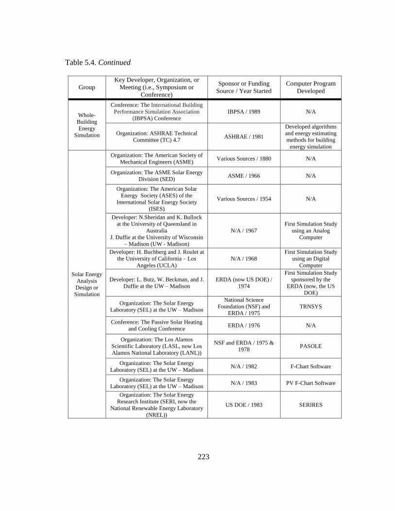
223

Table 5.4. Continued

Group

Key Developer, Organization, or

Meeting (i.e., Symposium or

Conference)

Sponsor or Funding

Source / Year Started

Computer Program

Developed

Whole-

Building

Energy

Simulation

Conference: The International Building

Performance Simulation Association

(IBPSA) Conference

IBPSA / 1989 N/A

Organization: ASHRAE Technical

Committee (TC) 4.7 ASHRAE / 1981

Developed algorithms

and energy estimating

methods for building

energy simulation

Solar Energy

Analysis

Design or

Simulation

Organization: The American Society of

Mechanical Engineers (ASME) Various Sources / 1880 N/A

Organization: The ASME Solar Energy

Division (SED) ASME / 1966 N/A

Organization: The American Solar

Energy Society (ASES) of the

International Solar Energy Society

(ISES)

Various Sources / 1954 N/A

Developer: N.Sheridan and K. Bullock

at the University of Queensland in

Australia

J. Duffie at the University of Wisconsin

– Madison (UW - Madison)

N/A / 1967

First Simulation Study

using an Analog

Computer

Developer: H. Buchberg and J. Roulet at

the University of California – Los

Angeles (UCLA)

N/A / 1968

First Simulation Study

using an Digital

Computer

Developer: L. Butz, W. Beckman, and J.

Duffie at the UW – Madison

ERDA (now US DOE) /

1974

First Simulation Study

sponsored by the

ERDA (now, the US

DOE)

Organization: The Solar Energy

Laboratory (SEL) at the UW – Madison

National Science

Foundation (NSF) and

ERDA / 1975

TRNSYS

Conference: The Passive Solar Heating

and Cooling Conference ERDA / 1976 N/A

Organization: The Los Alamos

Scientific Laboratory (LASL, now Los

Alamos National Laboratory (LANL))

NSF and ERDA / 1975 &

1978 PASOLE

Organization: The Solar Energy

Laboratory (SEL) at the UW – Madison N/A / 1982 F-Chart Software

Organization: The Solar Energy

Laboratory (SEL) at the UW – Madison N/A / 1983 PV F-Chart Software

Organization: The Solar Energy

Research Institute (SERI, now the

National Renewable Energy Laboratory

(NREL))

US DOE / 1983 SERIRES

224

Table 5.4. Continued

Group

Key Developer, Organization, or

Meeting (i.e., Symposium or

Conference)

Sponsor or Funding

Source / Year Started

Computer Program

Developed

Solar Energy

Analysis

Design or

Simulation

Organization: The Sandia National

Laboratory (SNL) US DOE / 1985 PVFORM model

Organization: The CSU and NREL (i.e.,

formerly SERI) US DOE / 1996 SUNREL

Lighting &

Daylighting

Analysis

Simulation

Organization: The Illuminating

Engineering Society of North America

(IESNA) of the Illuminating

Engineering Society (IES)

Various Sources / 1906 N/A

Developer: R. Hopkinson, J. Longmore,

and P. Petherbridge at the Building

Research Station in the U.K.

N/A / 1954

Split Flux Method,

later Used for the

DOE-2 Daylighting

Model

Developer: E. Sparrow at the University

of Minnesota and R. Cess at the State

University of New York at Stony Brook

N/A / 1966

Radiosity Method,

later Used for

SUPERLITE and

DElight Version 2.0

(i.e. the EnergyPlus

Daylighting Module)

Developer: Arthur Appel at the IBM

Research Center N/A / 1967

Ray Tracing Method,

later Used for

Radiance

Developer: David DiLaura at Wayne

State University N/A / 1968

Lumen I

(later became Lumen

Micro)

Conference: The Association for

Computing Machinery (ACM)’s Special

Interest Group on Graphics and

Interactive Techniques (SIGGRAPH)

Conference

ACM / 1974 N/A

Organization: LBL (now LBNL) US DOE / 1982 The DOE-2

Daylighting model

Organization: LBL US DOE / 1982 SUPERLITE

Developer: Gregory Ward at the LBL

and the Ecole Polytechnique Federal de

Lausanne (EPFL, Swiss institute)

US DOE and the Swiss

government / 1989 Radiance

Organization: LBNL (formerly LBL) US DOE / 2003 or 2004

DElight Version 2.0

(i.e., the EnergyPlus

Daylighting Module)

In this section, the key developers or institutes are categorized by organization

for the whole-building energy simulation programs, solar energy analysis programs, and

the lighting and daylighting analysis programs.

225

5.4.1 The organizations for developing whole-building simulation programs

The most important engineering organization that contributed to the development

of whole-building simulation programs in the U.S. is the American Society of Heating,

Refrigerating and Air Conditioning Engineers (ASHRAE).

In 1889, the Master Steam and Hot Water Fitters Association of the United States

(i.e., the antecedent of the American Society of Heating and Ventilating engineers

(ASHVE)) was organized and opened the first convention of the Master Fitters

Association. In 1894, ASHVE was started by the contribution of Hugh Barron who

wanted to improve the convention by focusing on technical issues other than business of

interest. In 1904, another engineering association, the American Society of Refrigerating

Engineers (ASRE), was established by William Ross. He organized ASRE under the

idea caused from an industry journal, the Cold Storage and Ice Trade Journal

(Donaldson et al., 1994; ASHRAE, 2013).

In 1954, the name of ASHVE was changed to the American Society of Heating

and Air Conditioning Engineers (ASHAE). In 1958, the members of ASHAE and ASRE

voted to merge the two organizations. Finally, in 1959, the merged organization was

officially launched with a new name, ASHRAE (ASHRAE, 2013).

Until the 1960s, most engineers estimated heating and cooling energy used in a

building by using approximate methods from experience such as the heating degree day

method, the bin method, and the cooling degree day method (i.e., equivalent full-load

hour method) (Tull, 1971; Stamper, 1995). However, accurate methods were required to

calculate heating and cooling energy because the heating and cooling energy cost

226

accounts for the substantial amount of the total energy cost in a building. In addition, the

use of a computer was necessary because an accurate energy estimation was complicated

due to the effects of the varying weather data, HVAC system performance, and HVAC

operating schedules (Tull, 1971).

In 1965, ASHRAE founded a Presidential Committee on Energy Consumption

according to the significance of calculating heating and cooling energy with accurate

methods. This committee checked the issues of developing accurate methods in detail

and suggested assignments to a task group, called Task Group on Load Profiles, founded

in 1965. From 1965 to 1966, the initial Task Group researched the accurate methods and

developed a diagram for estimating building load profiles (Tull, 1971; Stamper, 1995).

In 1966, the Task Group voted for the budgets for energy calculation research projects

and a new renamed Task Group (Stamper, 1995). In 1967, the new Task Group known

as the ASHRAE Task Group on Energy Requirements (TGER) for Heating and Cooling

Buildings held the first meeting. Robert Tull, who was a previous ASHRAE president,

became the chairman of the ASHRAE TGER (Tull, 1971; Stamper, 1995; Kusuda,

1999). In the mid-1960s, other engineering groups such as Westinghouse Electric

Company, a group of gas industry companies called Group to Advance Total Energy

(GATE), and Automated Procedures for Engineering Consultants (APEC) also

developed computer procedures to calculate building energy. The ASHRAE TGER

decided to utilize the computer procedures developed from other engineering groups to

develop new computer algorithms (Tull, 1971; Stamper, 1995). At the time, engineers

needed open source algorithms because some existing procedures of the groups were

227

proprietary (Stamper, 1995). The National Bureau of Standards (NBS, now NIST), the

U.S. Postal Service (USPS) and the National Research Council of Canada (NRC) also

have contributed to the Task Group’s project (Tull, 1971).

The ASHRAE TGER consisted of four subcommittees. Subcommittee #1 on

Heating and Cooling Load Requirements was in charge of developing building loads

calculation procedures. Subcommittee #2 on System and Equipment Energy was

responsible for creating a new method to calculate energy requirements of HVAC

systems and plants by utilizing the building loads. Subcommittee #3 on the Overall

Logic Pattern worked for integrating other affecting variables, such as weather,

operation schedule, and system auxiliaries, with the building loads and energy

requirements calculations. Subcommittee #4 on Field Validation Studies was in charge

of validating the developed procedures (Tull, 1971).

The ASHRAE TGER developed algorithms for calculating building loads that

implemented a non-steady state heat calculation method developed by Stephenson and

Mitalas in 1967 instead of the Total Equivalent Temperature Difference (TETD) / Time

Averaging (TA) method described in the 1967 ASHRAE fundamental handbook.

Stephenson and Mitalas’s method, called the Thermal Response Factor Method, was

used for calculating the instantaneous heat conduction through walls and roofs. This

method discussed in Section 5.2.1.2 was also used for approximately calculating the

thermal storage effect for walls and roofs. In 1968 and 1969, ASHRAE TGER first

released two books that contained the algorithms of the building loads calculation

methods of buildings and the energy calculation methods of HVAC systems and plants.

228

The loads calculation book was restrictively distributed to researchers and engineers at

the ASHRAE annual meeting in 1968. The system simulation book was released in

1969. This book also was narrowly distributed (Tull, 1971).

In 1970, the first symposium regarding the use of computers for building energy

simulation was held at the National Bureau of Standards (NBS) in Gaithersburg,

Maryland, titled “Use of Computers for Environmental Engineering Related to

Buildings” (Kusuda ed., 1971). This symposium attracted approximately 400 architects,

engineers, and scientists from 12 countries. The 59 technical papers of this symposium

addressed issues including computer applications for building heat transfer analysis,

loads and energy calculations, HVAC system simulations, weather data, and computer

graphics. The majority of these proceedings was related to cooling and heating load

calculations because these were popular topics among building environmental engineers

in the late 1960s (Kusuda ed., 1971). The application of computers to dynamic thermal

load calculations allowed building engineers to work with more accurate solutions and

methods (Tull, 1971; Lokmanhekim, 1971).

In 1971, the USPS held a symposium to introduce a Post Office computer

program (USPS, 1971). The USPS developed the Post Office program, called Computer

Program for Analysis of Energy Utilization in Postal Facilities, to calculate building

energy savings for increasing post office branches. In the 1970s, the USPS was the

second ranking institute that built many buildings in the U.S. (USPS, 1971; Stamper,

1995). The General American Research Division (GARD) of the General American

Transportation Corporation (GATX), which was a subcontractor for the Post Office

229

facilities division, developed the loads program (i.e., computational procedures) for the

Post Office Program (Stamper 1995; Cumali, 2013).

In 1973, oil crisis from an Arab embargo as well as advanced computers

triggered progressive improvements of developing computer procedures that analyze

building thermal behavior and energy consumption (Ayres and Stamper, 1995). U.S.

government funding was moved to the building energy simulation program area from the

nuclear and aerospace technology area (Kusuda, 1999). The Energy Research and

Development Administration (ERDA) (now, the USDOE) and Lawrence Berkeley

Laboratory (LBL, now Lawrence Berkeley National Laboratory (LBNL)) developed

CAL-ERDA in 1976 based on the analysis method (i.e., the Weighting Factor Method

(WFM)) of the Post Office program. The Computation Consultants Bureau (CCB), the

Argonne Nation Laboratory (ANL), and the Los Alamos Scientific Laboratory (LASL,

now Los Alamos National Laboratory (LANL)) also contributed to the development of

CAL-ERDA (Graven and Hirsch, 1977). In 1979, CAL-ERDA became the DOE-2

version. In the mid-1980s, the funding from the US DOE had been quickly reduced at

ANL and LASL, so LBL became the main national laboratory for developing new

versions of DOE-2 (Ayres and Stamper, 1995).

The U.S. Department of Defense (DOD) supported and the U.S. Army

Construction Engineering Research Laboratory (CERL) issued BLAST in 1977 based on

the analysis method (i.e., the Heat Balance Method (HBM)) of the NBSLD program

developed at the NBS in the late 1960s (Stamper, 1995). In the meantime, proprietary

sectors also developed building energy simulation programs. The utility industry

230

released Gas for the Advancement of Total Energy (GATE) (later E-CUBE) in 1967 and

AXCESS in 1971, and APEC issued HCC and ESP in 1967 and 1978. The Trance

Company developed TRACE in 1972 (PNNL, 1990; Stamper, 1995; Ayres and Stamper,

1995). In 1996, DOE-2 and BLAST started to be combined as EnergyPlus by the efforts

of LBNL, CERL, University of Illinois at Urbana-Champaign (UIUC), Oklahoma State

University (OSU), GARD Analytics (formerly, GARD/GATX), and Florida Solar

Energy Center, which are sponsored by the US DOE (Crawley et al., 2002).

In 1974, 1978, and 1983, building energy simulation symposiums following the

first symposium for the use of computers for building energy simulation that was held in

1970 at the NBS were opened in Paris, Banff, and Tokyo. This is because the first

symposium at the NBS was successfully held and attracted substantial interest (Kusuda

ed., 1971; Kusuda, 1999). In 1985, the Building Energy Simulation Conference,

sponsored by the Passive Solar Group of the US DOE, was held in Seattle, Washington

(US DOE, 1985). The previous four symposiums and the one conference were

considered as the origins of the International Building Performance Simulation

Association (IBPSA) conference, which has been now opened every two years since

1989 (Kusuda, 1999). The IBPSA was established in 1987 to develop and share practical

and advanced knowledge for building energy simulation worldwide (Tupper et al.,

2011).

The ASHRAE TGER became Technical Committee (TC) 4.7 (ASHRAE, 1981;

Stamper, 1995). TC 4.7 has contributed to the development of building energy

231

simulation and the building energy estimating methods for simulation such as

EnergyPlus until now.

In summary, the ASHRAE TGER was the main contributor for developing the

algorithms of building energy simulation. Currently, TC 4.7, formerly the ASHRAE

TGER, is the main supplier for the algorithms and estimating methods of building

energy simulation. The US DOE, US DOD, USPS, and NBS (now NIST) contributed to

the development of simulation programs based on the algorithms of the ASHRAE

TFGER. National laboratories (i.e., LBL, ANL, and LASL) and consultant and academic

institutes (i.e., CCB, GARD Analytics, UIUC, and OSU) also contributed to the

development. The first symposium at the NBS successfully continues to the present time

as the IBPSA conference.

5.4.2 The organizations for developing solar system analysis simulation programs

The American Society of Mechanical Engineers (ASME) Solar Energy Division

(SED) and the American Solar Energy Society (ASES) have been the major contributors

for the development of solar system analysis simulation programs.

In 1880, the ASME was founded to enhance and to share mechanical technology

(ASME, 2013a). In the mid-1950s, mechanical engineers at the Massachusetts Institute

of Technology (MIT) started to study reliable solar energy systems. Hottel and Woertz

published their paper in Transactions of ASME (Hottel and Woertz, 1942; Balcomb,

1992; Beckman, 1993). In 1960, the Journal of Solar Energy Engineering was started.

This journal has allowed many solar engineers to be involved in solar technology and

simulation development (ASME, 2013b). In 1966, the ASME SED was grouped from

232

the ASME to effectively utilize mechanical systems for solar energy (ASME, 2013c). In

addition, the ASME Solar Energy Conference was started in 1981 for sharing

information between solar engineers. This conference was integrated by previous

conferences (i.e., the System Simulation and Economic Analysis (SSEA) Conference

and the Solar Heating and Cooling Operational Results (SHCOR) Conference)

sponsored by US DOE. The SSEA conference, held in 1978 and 1980, dealt with the

issues of system simulation and economics. The SHCOR, held in 1978 and 1979,

covered active and passive solar systems (Reid, 1981).

The ASES was founded in 1954. The ASES has increased solar energy feasibility

as one of the sections of the International Solar Energy Society (ISES) (ASES, 2012).

Solar Energy has been a journal of the ISES since 1957 and this journal also allowed

many solar engineers to be involved in solar technology and simulation development

(ELSEVIER, 2013). The ISES conference has been held every two years since the 1950s

for solar engineers (ISES, 2012).

In 1967, N. Sheridan and K. Bullock at the University of Queensland in Australia

and J. Duffie at the University of Wisconsin – Madison first studied simulation for solar

systems. The researchers studied a process between solar water heating system

components by using an analog computer (Sheridan et al., 1967; Beckman, 1993). In the

same year, Close at the UW – Madison extended the previous study using an analog

computer to an improved study using a digital computer with an analog simulation

program. He proposed a factorial design method for estimating the effects of solar water

heaters (Close, 1967). Early studies were conducted by using analog simulation because

233

electrical models were able to easily account for the physical systems. However, analytic

weather data was used and annual analysis could not be studied by analog simulation

due to high cost (Beckman, 1993). In 1968, H. Buchberg and J. Roulet at University of

California – Los Angeles (UCLA) used real weather data for annual simulation by using

digital computer programs for estimating the effects of solar collector, storage, and

auxiliary systems in residential buildings. IBM 7094 (i.e., a digital computer) located at

UCLA was used for all computations in this study (Buchberg and Roulet, 1968). In

1973, G. Löf at Ohio State University (OSU) and R. Tybout at Colorado State University

(CSU) first studied solar heating systems with a practical “what if” approach. They

selected eight cities in the U.S. and hourly analyzed solar heating systems with several

parameters, such as house, collector, storage sizes, tilted angle of solar collectors, and

collector thermal capacity, using the speed of a digital computer (Löf and Tybout, 1973;

Beckman, 1993). All the papers above were published in Solar Engineering journals of

ISES.

Before 1973, solar simulation research was conducted by different universities

and institutes, showing a lack of coherence between researches. In 1972, the national

scheme for solar energy employment was proposed by the National Science Foundation

(NSF) (Beckman, 1993). In 1974, the first study for solar simulation under the

sponsorship of the U. S. Energy Research and Development Administration (ERDA,

now the U. S. Department of Energy (US DOE)) was conducted by L. Butz, W.

Beckman, and J. Duffie at the UW – Madison for solar cooling and heating systems of

residential buildings (Butz et al., 1974; Beckman, 1993). About the same time, CSU

234

researchers tried to build a test house for estimating solar heating systems, supported by

the NSF. The simulation code of the Butz et al.’s program showed the deficiency of

analyzing the CSU’s solar test house. This was because the flexibility of the simulation

code was inefficient to analyze the design parameters of the test house even though the

solar heating systems of Butz et al’s study were parallel to those of the CSU’s solar test

house (Beckman, 1993). The need of a flexible program created a simulation program

with a modular approach. The Solar Energy Laboratory (SEL) at the UW – Madison

proposed this development plan of the simulation program to the NSF. In 1975, a new

developed simulation code became the modular simulation program, TRNSYS under the

sponsorship of the NSF and the ERDA (Klein, 1976; Beckman, 1993; Tupper et al.,

2011).

Other simulation programs were developed at the Los Alamos Scientific

Laboratory (LASL, now Los Alamos National Laboratory (LANL)), by the sponsorship

of the NSF and the US DOE programs (Kusuda, 1985; Beckman, 1993). The LASL

programs were not fully documented and used as research tools (Beckman 1993). One of

the LASL programs was PASOLE, and the name was from PAssive SOLar Energy. This

simulation program was used in aiding to create design methods for passive solar heating

applications (McFarland, 1978; Feldman and Merriam, 1979).

In 1976, the first strong interest for passive solar systems was represented as the

Passive Solar Heating and Cooling conference, which was held at the University of New

Mexico (LASL, 1976; Balcomb, 1992). The ERDA sponsored this conference, and the

LASL coordinated it in collaboration with the American Society of Heating,

235

Refrigerating and Air Conditioning Engineers (ASHRAE) and the New Mexico Solar

Energy Association (NMSEA) (LASL, 1976). In 1977 and 1978, the ASES of ISES also

held a conference for passive solar systems, sponsored by the US DOE (Prowler ed.,

1978).

In 1979, Arthur D. Little, Inc. engineers including Feldman and Merriam

reviewed approximately 70 simulation programs. The report of Arthur D. Little, Inc. was

sponsored by Electric Power Research Institute (EPRI). The Solar Energy Research

Institute (SERI, now the National Renewable Energy Laboratory (NREL)) and the US

DOE coordinated this review report due to mutual interests (Feldman and Merriam,

1979). The SERI published a brochure with the updated list of solar simulation programs

based on EPRI’s report (SERI, 1980).

In 1983, The SERI developed the SERIRES simulation program for buildings

that have passive solar systems. SERIRES stands for Solar Energy Research Institute

Residential Energy Simulator (Palmiter and Wheeling, 1983). In 1985, the Sandia

National Laboratory (SNL) developed a PVFORM model (i.e., detailed model) for

photovoltaic (PV) systems used in most detailed PV programs in the U.S. (Menicucci,

1985; Klise and Stein, 2009). In 1996, SERIRES was upgraded to SUNREL by CSU and

NREL (i.e., formerly SERI) (Deru, 1996). In 2009, the SEL published a review report

for PV simulation programs (Klise and Stein, 2009).

In summary, the SED of ASES and the ASES of ISES have been the major

contributors in the U.S. for the development of solar energy technology and simulation

programs. From 1972, the US DOE financially supported most of the simulation

236

development of solar energy systems. National laboratories (i.e., LASL (now, LANL),

SERI (now, NREL), and SNL), and universities (i.e., the UW – Madison and CSU),

institutes (i.e., EPRI and NMSEA) conducted studies for the simulation development

under the sponsorship of the US DOE.

5.4.3 The organizations for developing lighting and daylighting analysis simulation

programs

The Illuminating Engineering Society (IES) and the Illuminating Engineering

Society of North America (IESNA), which were established in 1906, have contributed to

the development of lighting and daylighting technology. In the same year, the Journal of

the Illuminating Engineering Society was started and published every year since 1906

(DiLaura, 2006). The ASES and ISES have also enhanced lighting and daylighting

technology. The journal of Solar Energy by the ISES was started in 1957 and this journal

also allowed many lighting and daylighting engineers to be involved in lighting and

daylighting technology and simulation development (ISES, 2012).

In 1954, 1966, and 1968, key methods for calculating internal reflected light

were introduced. In 1954, the split flux method was proposed by R. Hopkinson, J.

Longmore, and P. Petherbridge at the Building Research Station (BRS) in the U.K.

(Hopkinson et al., 1954). In 1966, E. Sparrow at the University of Minnesota and R.

Cess at the State University of New York at Stony Brook introduced the radiosity

concept in their book (Sparrow and Cess, 1966). In 1967, Arthur Appel at the IBM

Research Center first proposed the concept of ray tracing (Appel, 1967; Weghorst et al.,

1984).

237

In 1968, David DiLaura at Wayne State University proposed the Lumen I

program that can estimate artificial lighting systems based on point-by-point calculations.

In 1970, DiLaura developed Lumen II. This program improved the existing capabilities

of Lumen I by adding the estimation options of daylighting, glare, and visual comfort. In

1980, DiLaura established Lighting Technologies Inc., and Lumen III was developed at

Lighting Technologies Inc. in 1981. In 1983, Lighting Technologies Inc. released the

first version of Lumen Micro, which was the next version of the Lumen series (i.e.,

Lumen I, II, and III). The name of Lumen Micro reflected the use of a microcomputer

(as cited in Kota and Haberl, 2009). In the late 1980s, Lighting Technologies Inc. added

a daylighting module to Lumen Micro. In 1996 and 1998, Lumen Micro Version 7.1 and

Version 7.5 were released (Ubbelohde and Humann, 1998).

In 1969, the Special Interest Group on Graphics and Interactive Techniques

(SIGGRAPH) was grouped from the Association for Computing Machinery (ACM)

established in1947 (Williams, 1998; ACM, 2013). In 1974, a SIGGRAPH conference

was initiated and has been held every year since 1974 (Williams, 1998). The

SIGGRAPH and conference have been an important role for the development of lighting

and daylighting simulation because the simulation analysis was related to rendering

issues (i.e., image generation) based on computer graphics (Ward, 1994).

In the U.S. around 1976, strong interest and effort for employing passive solar

energy were initiated (Balcomb, 1992). In 1976, the Passive Solar Heating and Cooling

conference, which was discussed in the previous section, was held by the coordination of

the LASL and the sponsorship of the ERDA (LASL, 1976; Balcomb, 1992). The interest

238

of passive solar energy stimulated daylighting utilization because daylighting could be

employed as a major approach of passive solar technology. In addition, daylighting

utilization was able to accomplish building energy savings due to the reduction of

electrical light usage (Gordon et al., 1986).

In 1982, LBL (now LBNL) researchers developed a daylighting model using the

split flux method introduced in 1954. They integrated the daylighting model with the

DOE-2.1b program (i.e., the building loads analysis program) to analyze the energy

effects of the daylighting utilization in buildings (Selkowitz et al., 1982; LBL, 1982;

Winkelmann, 1983). This model has been applied to the DOE-2.1 program series since

1982. In the same year, Michael Modest at University of Southern California (USC)

published a paper to describe computer algorithms using the radiosity method introduced

in 1966. The algorithms for digital computers were developed to calculate the

daylighting effects inside rooms in buildings (Modest, 1982). Also, in the same year,

Stephen Selkowitz, Jong-Jin Kim, Mojtaba Navvab, and Frederick Winkelmann at LBL

described and compared the DOE-2.1 daylighting model and SUPERLITE (Selkowitz et

al., 1982). In 1984, Cindy Goral, Kenneth Torrance, Donald Greenberg, and Bennett

Battaile at Cornell University first represented the radiosity method for computer

graphics (Goral et al., 1984).

In around 2003, NBNL developed a DElight Version 2.0 program that was the

next version of SUPERLITE using the radiosity method. Before Version 2.0, Version

1.X series adopted the daylighting algorithms of the DOE-2.1b using the split flux

method (Hitchcock and Carroll, 2003). In 2004, University of Illinois at Urbana-

239

Champaign (UIUC) and LBNL researchers integrated the version 2.0 of DElight into the

EnergyPlus Version 1.2. From 2004, the DElight has been combined with the following

versions of EnergyPlus (EERE, n.d.).

In 1989, Radiance using the ray tracing method introduced in 1968 was first

released by the effort of Gregory Ward at the LBL and the Ecole Polytechnique Federal

de Lausanne (EPFL, Swiss institute) (Ward, 1994). In 1998, Christoph Reinhart led the

development of DAYSIM based on the Radiance algorithms. The National Research

Council (NRC) Canada, Fraunhofer Institute for Solar Energy Systems (FISE), Harvard

University, and Massachusetts Institute of Technology (MIT) contributed the

development of DAYSIM (Reinhart, 2013). Since the years, Radiance and DAYSIM

have been widely used for lighting and daylighting analysis.

In summary, the Illuminating Engineering Society of North America (IESNA),

which was established in 1906, was a main contributor for developing lighting and

daylighting technology in the U.S. In the 1950s and 1960s, many researchers (i.e.,

Hopkinson, Longmore, Patherbridge, Sparrow, Cess, Appel, and DiLaura) developed

key lighting and daylighting analysis methods that were later used for simulation

programs. After 1976 when there was strong national interest for employing daylighting

strategies, LBL (now LBNL) has been a major developer for lighting and daylighting

simulation (i.e., the DOE-2.1 daylighting algorithms, SUPERLITE, DElight, and

Radiance).

240

CHAPTER VI

SUMMARY

Throughout this study, the origins of the key analysis methods used in whole-

building simulation programs, solar energy design and simulation programs, and lighting

and daylighting simulation programs, which were developed in the U.S., were traced and

analyzed. In addition, the origins of the selected simulation programs and the

organizations who contributed to the development of the analysis methods and the

simulation programs were traced and analyzed. As a result, a new comprehensive

genealogy chart has been created as shown in Appendix A, which is discussed using four

approaches: by time period, analysis method, simulation program, and funding or

organization. This study is intended to give readers a better understanding of where the

analysis methods of the simulation programs came from, who developed them, and why

they were developed through tracing the origins of the simulation programs.

The observations and findings from this study are the following:

Summary by time period:

Significant historical events such as World War I (1914-1918) and World War II

(1939-1945), the development of analog and digital computers and programming

languages (1950s), and repeated oil crises (1967, 1973, and 1979) had a major

impact on the development of key analysis methods and the origins of the

simulation programs that are now used to simulate annual building energy use.

241

In the pre-1950s period, most fundamentals (i.e., gas laws, heat transfer

properties, and thermodynamics) of HVAC systems were studied and published,

which contributed significantly to the development of today’s technology. Also,

during this same period, researchers and engineers developed the essential

methods for: calculating dynamic heat gain and building loads (i.e., cooling and

heating loads) used in whole-building energy simulation programs; calculating

solar heating performance prediction used in solar energy analysis design and

simulation programs; and for analyzing internal reflected illuminance used in

lighting and daylighting simulation programs.

During the 1950s, analog computers were widely used to study the behavior of

dynamic heat gain/loss and the response of heating, ventilating, and air

conditioning (HVAC) systems.

From the 1960s until the present, digital computers and analysis methods suitable

for the digital computers were developed and became widely used. Digital

computers were substituted for analog computers because the digital computer is

more convenient to program, more flexible, and the methods used in digital

computers made it easier and quicker to describe the governing equations and

driving functions than the methods used in analog computers. Finally, the

scientific applications of the digital computer was considerably improved by the

FORTRAN programming language, a high level scientific programming

language that was first commercially released in 1957 by IBM. FORTRAN also

allowed computer codes written on one computer to be run on another computer

242

by a different analyst, which accelerated the availability of simulation programs.

As a result, both analog and digital computers significantly contributed to the

development of whole-building, solar energy, lighting and daylighting simulation

programs.

Summary by analysis method:

In the 1920s, one of the most important methods for calculating the dynamic heat

gain through walls and roofs for whole-building energy simulation (i.e., the

Response Factor Method (RFM)) was developed and published by André Nessi

and Léon Nisolle at Ėcole Centrale Paris (French University) in France. The

RFM concept is still used in most of today’s cooling and heating loads

calculations such as with the Weighting Factor Method or the Transfer Function

Method for DOE-2.1e, DOE 2.2/eQUEST, TRACE, and HAP, the CLTD/CLF

method for TRACE, the Heat Balance method for BLAST and EnergyPlus, and

the Radiant Time Series Method for TRACE.

In the 1940s, the origin of the Resistance-Capacitance (RC) network analysis

method (i.e., the thermal network method) used in simulation programs for

buildings was first introduced by Victor Paschkis, a research engineer at

Columbia University. The thermal network concept is used today in whole-

building simulation programs such as DOE-2.1e and EnergyPlus and detailed

solar simulation programs such as TRNSYS and SUNREL.

243

In the 1950s, the origin of the most important method (i.e, the utilizability

method) for calculating the performance of solar heating systems for design or

simulation programs was developed by Austin Whillier at MIT. The utilizability

method is used today in both advanced solar energy simulation programs such as

TRNSYS and simplified solar design programs such as the F-Chart and the PV

F-Chart program.

In the 1950s and 1960s, the origins of the Inter Reflected Component (IRC)

calculation method (i.e., the split flux method, the radiosity method, and the ray

tracing method) for daylighting simulation were developed. In 1954, the split

flux method was proposed by R. Hopkinson, J. Longmore, and P. Petherbridge at

the Building Research Station in the U.K. In 1966, E. Sparrow at the University

of Minnesota and R. Cess at the State University of New York at Stony Brook

introduced the radiosity concept in their book, entitled Radiation Heat Transfer.

In 1967, Arthur Appel at the IBM Research Center first proposed the concept of

ray tracing. Today, the split flux method method is used in whole-building

energy simulation programs such as DOE-2.1e, DOE 2.2/eQUEST, and

EnergyPlus as a daylighting module. The radiosity method is used in Lumen

Micro and one of the dayligihtg modules of EnergyPlus. Finally, the ray-tracing

method is used in an advanced lighting and daylighting simulation program such

as Radiance.

244

Summary by simulation program

During the 1970s, companies and government organizations created dozens of

peak-load and annual energy use simulation programs due to the repeated energy

crises (1967, 1973, and 1979), the availability of digital computers, and the

development of FORTRAN. However, many of these simulation programs are no

longer in use because of a lack of support, poor documentation, limited technical

upgrades, or discontinuance of the program.

Today’s most widely used simulation programs are the following:

o a) whole-building energy simulation: EnergyPlus, DOE-2.1e, DOE-

2.2/eQUEST, TRNSYS, TRACE, and HAP;

o b) detailed solar energy simulation: TRNSYS and SUNREL, simplified

solar design analysis: the F-Chart program and the PV F- Chart program;

and

o c) Independent lighting and daylighting simulation programs: Radiance,

DAYSIM, and Lumen Micro; Integrated lighting and daylighting

simulation programs: the DOE-2 daylighting model and the EnergyPlus

daylighting modules.

Summary by organization and conference

Over the years, ASHRAE has led the development of the analysis methods and

the algorithms for whole-building energy simulation in the U.S. Most

developments of whole-building simulation programs have been conducted by

245

governmental organizations (i.e., US DOE, US DOD, USPS, and NIST),

engineering societies (i.e., ASHRAE and IBPSA), national laboratories (i.e.,

LBNL, ANL, and LANL), and consultant and academic institutes (i.e., CCB,

GARD Analytics, UIUC, and OSU).

In 1970, the first symposium regarding the use of computers for building energy

simulation was held at the NBS (now, NIST) in Gaithersburg, Maryland. In

1985, the Building Energy Simulation Conference, sponsored by the Passive

Solar Group of the US DOE, was held in Seattle, Washington (US DOE, 1985).

Both of these events are considered as the origins of the International Building

Performance Simulation Association (IBPSA) conference, which has been held

every two years since 1989.

The SED of ASES, established in 1966, and the ASES of ISES, established in

1954, have been the major organizers of conferences in the U.S. that reported on

the development of solar energy technology and simulation programs. From 1972

onward, the ERDA (now, the US DOE) financially supported the development of

simulation of solar energy systems. National laboratories (i.e., LANL, NREL,

and SNL), and universities (i.e., the UW – Madison and CSU) conducted

important studies that led to simulation development under the sponsorship of the

US DOE.

The Illuminating Engineering Society of North America (IESNA), established in

1906, was the main organizer of conferences that reported on the development of

lighting and daylighting technology in the U.S. In the 1950s and 1960s, many

246

researchers (i.e., Hopkinson, Longmore, Patherbridge, Sparrow, Cess, Appel, and

DiLaura) developed key lighting and daylighting analysis methods that were later

used for simulation programs. After 1976 when there was a strong national

interest for employing daylighting strategies, LBNL became the major developer

for lighting and daylighting simulation.

Key analysis methods developed by specific individuals at a variety of

organizations can be traced to today’s most widely used simulation programs.

The Total Equivalent Temperature Differential (TETD)/Time Averaging (TA)

method, the Transfer Function Method (TFM), the Cooling Load Temperature

Difference (CLTD)/Solar Cooling Load (SCL)/Cooling Load Factor (CLF)

method, and the Radiant Time Series (RTS) method were developed to calculate

peak cooling load for whole-building energy simulation programs. The

Weighting Factor Method (WFM) and the Heat Balance Method (HBM) were

developed to calculate time-varying cooling load for energy analysis for whole-

building energy simulation programs.

The thermal network method was developed and used to analyze the time-

varying dynamic cooling load and to simulate solar energy systems.

The utilizability method and the un-utilizability method were developed to

analyze solar energy amount for use by solar energy design or simulation

programs.

247

The split flux method, the radiosity method, and the ray tracing method were

developed to analyze the inter-reflected lighting and daylighting in buildings for

lighting and daylighting simulation programs.

Currently, the most widely used computer simulation programs in the U.S. for

whole-building energy simulations are DOE-2.1e, eQUEST/DOE2.2, TRACE, HAP,

TRNSYS, and EnergyPlus. TRNSYS and SUNREL are the most popular programs used

for detailed solar energy analysis in buildings. TRNSYS is used to estimate solar

thermal, active and passive solar systems, while SUNREL is used to analyze passive

solar systems. The F-Chart program and the PV F-Chart program are both widely used

for simplified solar energy analysis. Daylighting models in EnergyPlus, DOE-2.1e, and

eQUEST/DOE2.2 are widely used to analyze daylighting in buildings and to estimate

reduced lighting by daylighting. Radiance and Lumen Micro are used to simulate

lighting and daylighting of buildings and render images for lighting and daylighting.

DAYSIM is used to analyze annual lighting and daylighitng in buildings.

These prevalent simulation programs have adopted the key analysis methods,

including the weighting factor method (WFM), the heat balance method (HBM), the

thermal network method, the utilizability method, the un-utilizability method, the split

flux method, the radiosity method, and the ray tracing method. The WFM is used in

DOE-2.1e, eQUEST/DOE2.2, TRACE, and HAP. The HBM is used in EnergyPlus. The

thermal network method is used in all whole-building and solar energy simulation

programs, excluding lighting and daylighting simulation programs. The utilizability

248

method and un-utilizability method are used in the F-Chart program, and the utilizability

method is used in the PV F-Chart program. The split flux method is used in the

daylighting model in DOE 2.1e, eQUEST/DOE2.2, and EnergyPlus. The radiosity

method is used in the daylighting model of EnergyPlus and Lumen Micro. The ray

tracing method is used in Radiance and DAYSIM. DAYSIM uses the algorithms of

Radiance.

Some simulation programs have adopted the same analysis methods because

these methods have proved to be reliable. These analysis methods all have strength and

weaknesses- some have detailed solutions at slower computation speeds, and while

others have simplified solutions at higher speeds.

In this study, the origins of the analysis methods and the simulation programs as

well as the developers and the organizations who contributed to or funded the

development of the analysis methods and the simulation programs have been discussed

in order to better understand the simulation programs based on the comprehensive

genealogy chart. The discussions based on the comprehensive genealogy chart provide

detailed information to identify and comprehend the simulation programs, their analysis

method, developers, and organizations. The new comprehensive genealogy chart can be

used to better understand the analysis methods and capabilities of the selected simulation

programs.

249

REFERENCES

Alford, J. S., Ryan, J. E., & Urban, F. O. (1939). Effect of heat storage and variation in

outdoor temperature and solar intensity on heat transfer through walls. ASHVE

Transactions, 45, 369-396.

American Solar Energy Society (ASES). (2012). About the American solar energy

society. Retrieved from http://www.ases.org/about-ases/

American Society of Heating, Refrigerating and Air-Conditioning Engineers

(ASHRAE). (1961). ASHRAE guide and data book 1961 fundamentals and

equipment. New York, NY: Author.

American Society of Heating, Refrigerating and Air-Conditioning Engineers

(ASHRAE). (1975a). Procedure for determining heating and cooling loads for

computerizing energy calculations - Algorithms for building heat transfer

subroutines. Atlanta, GA: Author.

American Society of Heating, Refrigerating and Air-Conditioning Engineers

(ASHRAE). (1975b). Procedures for simulating the performance of components

and systems for energy calculations. W.F. Stoecker, (Ed.). Atlanta, GA: Author.

American Society of Heating, Refrigerating and Air-Conditioning Engineers

(ASHRAE). (1981). ASHRAE Handbook: 1981 Fundamentals. Atlanta, GA:

Author.

American Society of Heating, Refrigerating and Air-Conditioning Engineers

(ASHRAE). (1997). ASHRAE Handbook: 1997 Fundamentals. Atlanta, GA:

Author.

250

American Society of Heating, Refrigerating and Air-Conditioning Engineers

(ASHRAE). (1998). A toolkit for primary HVAC system energy calculations.

Atlanta, GA: Author.

American Society of Heating, Refrigerating and Air-Conditioning Engineers

(ASHRAE). (2001). ASHRAE Handbook: 2001 Fundamentals. Atlanta, GA:

Author.

American Society of Heating, Refrigerating and Air-Conditioning Engineers

(ASHRAE). (2009). ASHRAE Handbook: 2009 Fundamentals. Atlanta, GA:

Author.

American Society of Heating, Refrigerating and Air-Conditioning Engineers

(ASHRAE). (2010). ANSI/ASHRAE/IESNA standard 90.1-2010, Energy

standard for buildings except low-rise residential buildings. Atlanta, GA: Author

American Society of Heating, Refrigerating and Air-Conditioning Engineers

(ASHRAE). (2011). ANSI/ASHRAE/USGBC/IES standard 189.1-2011, Standard

for the design of high-performance green buildings except low-rise residential

buildings. Atlanta, GA: Author.

American Society of Heating, Refrigerating and Air-Conditioning Engineers

(ASHRAE). (2013). The ASHRAE centennial: 100 years of progress. Retrieved

from www.ashrae.org/file%20library/doclib/public/200511311142_347

American Society of Mechanical Engineers (ASME). (2013a). About ASME. Retrieved

from https://www.asme.org/about-asme

251

American Society of Mechanical Engineers (ASME). (2013b). All issues. Retrieved from

http://solarenergyengineering.asmedigitalcollection.asme.org/issues.aspx

American Society of Mechanical Engineers (ASME). (2013c). Solar energy division.

Retrieved from http://divisions.asme.org/solar/

Anderson, J. V., Mitchell, J. W., & Beckman, W. A. (1980). A design method for

parallel solar-heat pump systems. Solar Energy, 25, 155-163.

Appel, A. (1967). The notion of quantitative invisibility and the machine rendering of

solids. Proceedings of the ACM National Conference, New York, NY, 387-393.

Arney, M., Seward, P., & Kreider, J. F. (1981). P-chart – a passive solar design method.

Energy Engineering, 78(3), 41-50.

Arvo, J. (1986). Backward ray tracing. SIGGRAPH ’86 Developments in Ray Tracing

Course notes, volume 12. Retrieved from

http://www.cs.washington.edu/education/courses/cse457/06au/projects/trace/extr

a/Backward.pdf

Association for Computing Machinery (ACM). (2013). History. Retrieved from

http://www.acm.org/about/history?searchterm=acm+established+1947

Athienitis, A., Kalogirou, S. A., & Candanedo, L. (2012). Modeling and simulation of

passive and active solar thermal systems. In A. Sayigh (Ed.), Comprehensive

Renewable Energy Volume III (pp. 357-417). New York, NY: ELSEVIER.

Ayres, J. M., & Stamper, E. (1995). Historical development of building energy

calculations. ASHRAE Transactions, 37(2), 841-849.

252

Balcomb, J. D. (1992). Introduction. In J. D. Balcomb (Ed.), Passive solar buildings (pp.

1-37). Cambridge, MA: The MIT Press.

Balcomb, J. D., & Hedstrom, J. C. (1976). A simplified method for calculating required

solar collector array size for space heating. Proceedings of ISES Annual Meeting,

Winnipeg, Canada, August 15-20, 280-294.

Balcomb, J. D., Jones, R. W., McFarland, R.D., & Wray, W. O. (1984). Passive solar

heating analysis: a design manual. Atlanta, GA: ASHRAE.

Balcomb, J. D., & McFarland, R. D. (1978). A simple empirical method for estimating

the performance of a passive solar heated building of the thermal storage wall

type. Proceedings of 2nd

National Passive Solar Conference, Philadelphia, PA,

March 16-18, 1-13.

Balcomb, J. D., & Wray, W. O. (1988). Passive solar heating analysis. Supplement one:

thermal mass effects and additional SLR correlations. Atlanta, GA: ASHRAE.

Barley, C. D., & Winn, C. B. (1978). Optimal sizing of solar collectors by the method of

relative areas. Solar Energy 21(4), 279-289.

Beckman, W. A. (1993). Detailed simulation methods and validation. In G. Löf (Ed.),

Active solar systems (pp. 19-38). Cambridge, MA: The MIT Press.

Beckman, W. A., Klein, S. A., & Duffie, J. A. (1977). Solar heating design by the f-

chart method. NY: John Wiley & Sons.

Bellis, M. (2013). The history of the ENIAC computer. Retrieved from

http://inventors.about.com/od/estartinventions/a/Eniac.htm

253

Bendt, P., Collares-Pereira, M., & Rabl, A. (1981). The frequency distribution of daily

insolation values. Solar Energy, 27(1), 1-5.

Birdsall, B., Buhl, W. F., Ellington, K. L., Erdem, A. E., & Winkelmann, F. C. (1990).

Overview of the DOE-2 building energy analysis program version 2.1 D (LBL-

19735, Rev. 1). Berkeley, CA: Lawrence Berkeley Laboratory.

Bourgeois, D., Reinhart, C. F., & Macdonald, I. (2006). Adding advanced behavioural

models in whole building energy simulation: a study on the total energy impact

of manual and automated lighting control. Energy and Buildings, 38(7), 814-823.

Brandemuehl, M. J., Gabel, S., & Andresen, I. (1993). A tookit for secondary HVAC

system energy calculations. Atlanta, GA: ASHRAE.

Braun, J. E., Klein, S. A., & Pearson, K. A. (1983). An improved design method for

solar water heating systems. Solar Energy, 31(6), 597-604.

Bryan, H. J., & Clear, R. D. (1980). A procedure for calculating interior daylight

illumination with a programmable hand calculator (LBL-11186). Retrieved from

http://ec2-54-235-160-58.compute-

1.amazonaws.com/fedora/repository/ir%3A81470

Buchberg, H. (1955). Electric analogue prediction of the thermal behavior of an

inhabitable enclosure. ASHVE Transactions 61, 339-386.

Buchberg, H. (1958). Cooling load from thermal network solutions. ASHVE

Transactions 64, 111-128.

Buchberg, H., & Roulet, J. R. (1968). Simulation and optimization of solar collection

and storage for house heating. Solar Energy, 12, 31-50.

254

Buckles, W. E., & Klein, S. A. (1980). Analysis of solar domestic hot water heaters.

Solar Energy, 25, 417-424.

Buhl, W. F., Erdem, A. E., Winkelmann, F. C., & Sowell, E. F. (1993). Recent

improvements in SPARK: Strong component decomposition, multivalued

objects, and praphical interface. Proceedings of Building Simulation ’93,

Adelaide, Australia, August 16-18, 283-290.

Butz, L. W., Beckman, W. A., & Duffie, J. A. (1974). Simulation of a solar heating and

cooling system. Solar Energy, 16, 129-136.

Cane, R. L. D. (1979). A “modified” bin method for estimating annual heating energy

requirements of residential air source heat pumps (DBR No. 910). Ottawa,

Canada: National Research Council Canada.

Carpenter, R. C. (1897). Method of proportioning direct radiation. ASHRAE

Transactions 3, 73-90.

Carpenter, R. C. (1907). Derivation of constants for building losses. ASHRAE

Transactions 13, 90-102.

Carrier Corporation. (1960). Handbook of air conditioning system design. NY: McGraw

– Hill.

Carrier Corporation. (2003). HAP Quick Reference Guide. Syracuse, NY: Carrier

Corporation.

Carrier Corporation. (2013). What’s new with HAP. Retrieved from

http://www.commercial.carrier.com/commercial/hvac/general/0,3053,CLI1_DIV

12_ETI3944,00.html.

255

Ceylan, H. T., & Myers, G. E. (1980). Long-time solutions to heat-conduction transients

with time-dependent inputs. Journal of Heat Transfer, 102(1), 115-120.

Chen, F., & Jiang, Y. (1999). Introduction of building environment designer’s simulation

toolkit (DeST). Proceedings of Building Simulation ’99, Kyoto, Japan, 1165-

1172.

Cho, S., & Haberl, J. S. (2006). A survey of high-performance office buildings in the

United States. Proceedgins of Symposium on Improving Building Systems in Hot

and Humid Climates, Orlando, FL, July 24-26.

Clark, D. R., Klein, S. A., & Beckman, W. A. (1983). Algorithm for evaluating the

hourly radiation utilizability function. Journal of Solar Energy Engineering,

105(3), 281-287.

Clark, D. R., Klein, S. A., & Beckman, W. A. (1984). A method for estimating the

performance of photovoltaic systems. Solar Energy, 33(6), 551-555.

Clarke, J. A. (1982). Documentation of the ESP-r system final grant report to SERC.

Glasgow, Scotland: University of Strathclyde.

Clarke, J. A. (2001). Energy simulation in building design. Oxford, England:

Butterworth and Heineman.

Close, D. J. (1967). A design approach for solar processes (A 1966 conference paper).

Solar Energy, 11(2), 112-122.

Collares-Pereira, M., & Rabl, A. (1979). Simple procedure for predicting long term

average performance of nonconcentrating and of concentrating solar collectors.

Solar Energy, 23(3), 235-253.

256

Collins. (2013). Digital computer. Retrieved from

http://www.collinsdictionary.com/dictionary/english/digital-computer

Computer History Museum (CHM). (2008). The Babbage engine. Retrieved from

http://www.computerhistory.org/babbage/history/

Cook, R. L., Porter, T., & Carpenter, L. (1984). Distributed ray tracing. Computer

Graphics, 18(3), 137-145.

Copeland, B. J. (Ed.). (2006). COLOSSUS – the secrets of Bletchley Park’s

codebreaking computers. NY: Oxford University Press.

Crawley, D. B., Hand, J. W., Kummert, M., & Griffith, B. T. (2005). Contrasting the

capabilities of building energy performance simulation programs. Retrieved

from http://gundog.lbl.gov/dirpubs/2005/05_compare.pdf

Crawley, D. B., Hand, J. W., Kummert, M., & Griffith, B. T. (2008). Contrasting the

capabilities of building energy performance simulation programs. Building and

Environment, 43(4), 661-673.

Crawley, D. B., Lawrie, L. K., Pedersen, C. O., Liesen, R. J., Fisher, D. E., Strand, R.

K., Taylor, R. D., Winkelmann, F. C., Buhl, W. F., Huang, Y. J., & Erdem, A. E.

(1999). EnergyPlus: A new generation building energy simulation program.

Proceedings of Renewable and Advanced Energy Systems for the 21st Century,

Maui, Hawaii, April 11-15.

Crawley, D. B., Lawrie, L. K., Pedersen, C. O., Winkelmann, F. C., Witte, M. J., Strand,

R. K., Liesen, R. J., Buhl, W. F., Huang, Y. J., Hnninger, R. H., Glazer, J.,

257

Fisher, D. E., & Shirey, D. (2002). EnergyPlus: New, capable, and linked.

Proceedings of the 2002 International Green Building Conference, Austin, TX.

Crawley, D. B., Lawrie, L. K., Pedersen, C. O., Winkelmann, F. C., Witte, M. J., Strand,

R. K., Liesen, R. J., Buhl, W. F., Huang, Y. J., Henninger, R. H., Glazer, J.,

Fisher, D. E., Shirey, D. B., Griffith, B. T., Ellis, P. G., & Gu, L. (2004).

EnergyPlus: An update. Proceedings of the SimBuild 2004 Conference, Boulder,

CO, August 4-6.

Crawley, D. B., Lawrie, L. K., Winkelmann, F. C., Buhl, W. F., Erdem, A. E., Pedersen,

C. O., Liesen, R. J., & Fisher, D. E. (1997). What next for building energy

simulation – A glimpse of the future. Proceedings of Building Simulation ’97,

Prague, Czech Repunblic, September 7-10, Volume II, 395-402.

Crawley, D. B., Lawrie, L. K., Winkelmann, F. C., & Pedersen, C. O. (2001).

EnergyPlus: New capabilities in a whole-building energy simulation program.

Proceedings of Building Simulation 2001, Rio de Janeiro, Brazil, August, 51-58.

Cumali, Z. O. (2012). Fast algorithms for EnergyPlus acceleration Phase I – 2012.

Unpublished manuscript, Optens, LLC, CA.

Cumali, Z. O. (February 12, 2013). Personal communication.

Cumail, Z. O., Sezgen, A. O., & Sullivan, R. (1979). Final report - passive solar

calculation methods (Report under Contract EM-78-C-01-5221 to US

Department of Energy). Oakland, CA: CCB/Cumali Associates.

258

Degelman, L. O. (1990). ENERCAL: A weather and building energy simulation model

using fast hour-by-hour algorithms. Proceedings of the 4th

National Conference

on Microcomputer Applications in Energy, Tucson, AZ, 15-22.

Degelman, L. O., & Andrade, G. (1986). A bibliography of available computer

programs in the area of heating, ventilating, air conditioning, and refrigeration.

Atlanta, GA: ASHRAE.

Delcroix, B., Kummert, M., Daoud, A., & Hiller, M. (2012). Conduction transfer

functions in TRNSYS multizone building model: Current implementation,

limitations and possible improvements. Proceedings of the Fifth National

Conference of IBPSA-USA, Madison, WI, 219-226.

Deru, M. P. (1996). Improvements to the SERIRES/SUNREL building energy simulation

program. (Master’s thesis). Fort Collins, CO: Colorado State University.

Deru, M. P., Judkoff, R., & Torcellini, P. (2002). SUNREL, Technical reference manual

(NREL/BK-550-30193). Golden, CO: National Renewable Energy Laboratory.

DiLaura, D. L. (1975). On the computation of equivalent sphere illumination. Journal of

the Illuminating Engineering Society, 4, 129-149.

DiLaura, D. L. (1976). On the computation of visual comfort probability. Journal of the

Illuminating Engineering Society, 5, 207-217.

DiLaura, D. L. (2006). A history of light and lighting: in celebration of the centenary of

the Illuminating Engineering Society of North America. New York, NY: The

Illuminating Engineering Society of North America.

259

DiLaura, D. L., & Hauser, G. A. (1978). On calculating the effects of daylighting in

interior spaces. Journal of the Illuminating Engineering Society, 7, 2-14.

Donaldson, B., Nagengast, B., & Meckler, G. (1994). Heat & cold: Mastering the great

indoors. Atlanta, GA: ASHRAE.

Dooijes, E. H., & Peek, H. Z. (2013). Analog computers. Retrieved from

http://www.science.uva.nl/museum/AnalogComputers.php

Dresler, A. (1954). The “reflected component” in daylighting design. Transactions of the

Illuminating Engineering Society, 19(2), 50-60.

Duffie, J. A. (1993). Overview of modeling and simulation. In G. Löf (Ed.), Active solar

systems (pp. 3-18). Cambridge, MA: The MIT Press.

Duffie, J. A., & Beckman, W.A. (2006). Solar engineering of thermal processes. (3rd

ed.). Hoboken, NJ: John Wiley & Sons, Inc.

Einhorn, H. D. (1979). Discomfort glare: a formula to bridge differences. Lighting

Research and Technology, 11(2), 90-94.

ELSEVIER. (2013). Solar energy. Retrieved from

http://www.sciencedirect.com/science/journal/0038092X/1

Emery, A. F., Garbini, J. L., Heerwagen, D. R., Kunkle, R. D., & Kippenhan, C. J.

(1985). The measured performance and computer simulation of two unheated

passive solar test cells in the Pacific Northwest. Proceedings of Building Energy

Simulation Conference, Seattle, WA, 368-375.

260

Energy Efficiency & Renewable Energy (EERE). (n.d.). New features by EnergyPlus

version. Retrieved from

http://apps1.eere.energy.gov/buildings/energyplus/pdfs/featurehighlights.pdf

Energy Efficiency & Renewable Energy (EERE). (2010). EnergyPlus energy simulation

software. Retrieved from http://apps1.eere.energy.gov/buildings/energyplus/

Energy Efficiency & Renewable Energy (EERE). (2011a). Building energy software

tools directory: HAP. Retrieved from

http://apps1.eere.energy.gov/buildings/tools_directory/software.cfm/ID=385/pag

ename=alpha_list_sub

Energy Efficiency & Renewable Energy (EERE). (2011b). Building energy software

tools directory: SUNREL. Retrieved from

http://apps1.eere.energy.gov/buildings/tools_directory/software.cfm/ID=457/pag

ename=alpha_list_sub

Energy Efficiency & Renewable Energy (EERE). (2011c). Building energy software

tools directory: Radiance. Retrieved from

http://apps1.eere.energy.gov/buildings/tools_directory/software.cfm/ID=66/page

name=alpha_list_sub

Energy Efficiency & Renewable Energy (EERE). (2011d). Building energy software

tools directory: DAYSIM. Retrieved from

http://apps1.eere.energy.gov/buildings/tools_directory/software.cfm/ID=428/pag

ename=alpha_list_sub

261

Energy Efficiency & Renewable Energy (EERE). (2011e). EnergyPlus energy

simulation software. Retrieved from

http://apps1.eere.energy.gov/buildings/energyplus/

Energy Efficiency & Renewable Energy (EERE). (2012). EnergyPlus energy simulation

software. Retrieved from http://apps1.eere.energy.gov/buildings/energyplus/

Energy Efficiency & Renewable Energy (EERE). (2013a). Building energy software

tools directory. Retrieved from

http://apps1.eere.energy.gov/buildings/tools_directory/

Energy Efficiency & Renewable Energy (EERE). (2013b). EnergyPlus energy

simulation software. Retrieved from

http://apps1.eere.energy.gov/buildings/energyplus/

Energy Systems Research Unit. (2002). The ESP-r system for building energy

simulation, user guide version 10 series. Glasgow, Scotland: University of

Strathclyde.

Estes, J. M., Schreppler, S., & Newsom, T. (2004). Daylighting prediction software:

comparative analysis and application. Proceedgins of the Fourteenth Symposium

on Improving Building Systems in Hot and Humid Climates, Richardson, TX,

May 17-20, 259-267.

Evans, B. L., Klein, S. A., & Duffie, J. A. (1985). A design method for active-passive

hybrid space heating systems. Solar Energy, 35(2), 189-197.

262

Evans, D. L. (1980). Simplified method for predicting photovoltaic array output.

Proceedings of American Section Meeting of the International Solar Energy

Society, Phoenix, AZ, June 2-6.

Evans, D. L., Facinelli, W. A., & Koehler, L. P. (1980). Simulation and simplified design

studies of photovoltaic systems (SAND 80-7013). Albuquerque, NM: Sandia

National Laboratories.

Evans, D. L., Facinelli, W. A., & Otterbein, R. T. (1978). Combined

photovoltaic/thermal system studies (SAND 78-7031). Albuquerque, NM: Sandia

National Laboratories.

Evans, D. L., Rule, T. T., & Wood, B. D. (1982). A new look at long term collector

performance and utilizability. Solar Energy, 28(1), 13-23.

Farzad, M. (2012, January 13). Personal communication.

Faust, F. H., Levine, L., & Urban, F. O. (1935). A rational heat gain method for the

determination of air conditioning cooling loads. ASHVE Transactions, 41, 327-

354.

Feldman, S. J., & Merriam, R. L. (1979). Building energy analysis computer programs

with solar heating and cooling System capabilities (Research Report No. EPRI

ER-1146 to the Electric Power Research Institute). Cambridge, MA: Arthur D.

Little, Inc.

Fisher, D. E. (January 29, 2013). Personal communication.

Goldstein, R. A., & Nagel, R. (1971). 3-D visual simulation. Simulation, 16, 25-31.

263

Goral, C. M., Torrance, K. E., Greenberg, D. P., Battaile, B. (1984). Modeling the

interaction on light between diffuse surfaces. Proceedings of the 11th

Annual

Conference on Computer Graphics and Interactive Techniques SIGGRAPH ’84,

New York, NY, 213-222.

Gordon, H. T., Rittelman, P. R., Estoque, J., Hart, G. K., & Kantrowitz, M. (1986).

Passive solar energy for non-residential buildings. In K. W. Böer (Ed.), Advances

in solar energy – an annual review of research and development volume 3 (pp.

171-206). Boulder, CO: American Solar Energy Society (ASES), Inc.

Gough, M. A. (1999). A review of new techniques in building energy and environmental

modelling. Final Report BRE Contract No. BREA-42. Garston, Watford, UK:

Building Research Establishment.

Grantham, B. (2008). COEN 290 Computer Graphics I – Santa Clara University.

Retrieved from www.plunk.org/COEN-290/Notes/Week8.ppt

Gratia, E. (1985). The Sunspace: Computation and in-situ measures. Proceedings of the

Building Energy Simulation Conference, Seattle, WA, 338-345.

Graven, R. M., & Hirsch, P. R. (1977). CAL-ERDA users manual (ANL/ENG-77-03).

Argonne, IL: Argonne National Laboratory.

Greenberg, D. P., Cohen, M. F., & Torrance, K. E. (1986). Radiosity: A method for

computing global illumination. The Visual Computer, 2, 291-297.

Grondzik, W. T., Kwok, A. G., Stein, B., & Reynolds, J. S. (2010). Mechanical and

electrical equipment for buildings. Hoboken, NJ: John Wiley & Sons, Inc.

264

Gupta, Y., & Young, S. (1980). Method of predicting long-term average performance of

photovoltaic systems. Proceedings of Systems Simulation and Economic Analysis

Conference, San Diego, CA.

Haberl, J. S., & Cho, S. (2004a). Literature review of uncertainty of analysis methods

(F-Chart program) (ESL-TR- 04-08-04). Retrieved from Texas A&M

University, Energy Systems Laboratory website:

http://www.esl.tamu.edu/docs/terp/2004/ESL-TR-04-08-04.pdf

Haberl, J. S., & Cho, S. (2004b). Literature review of uncertainty of analysis methods

(PV F-Chart program) (ESL-TR-04-10-02). Retrieved from Texas A&M

University, Energy Systems Laboratory website:

http://www.esl.tamu.edu/docs/terp/2004/ESL-TR-04-10-02.pdf

Haberl, J. S., & Cho, S. (2004c). Literature review of uncertainty of analysis methods

(DOE-2 program) (ESL-TR- 04-11-01). Retrieved from Texas A&M University,

Energy Systems Laboratory website:

http://www.esl.tamu.edu/docs/terp/2004/ESL-TR-04-11-01.pdf

Harris, S. M., & McQuiston, F. C. (1988). A study to categorize walls and roofs on the

basis of thermal response. ASHRAE Transactions, 94(2), 688-714.

Hayashi, T., Urano, Y., Watanabe, T., & Ryu, Y. (1985). Passive system simulation

program "PSSP" and its applications. Proceedings of the Building Energy

Simulation Conference, Seattle, WA, 346-353.

265

Henninger, R. H. (Ed.). (1975). NECAP – NASA’s energy-cost analysis program: Part II

– engineering manual. NASA CR-2590 Part II. Washington, DC: National

Aeronautics and Space Administration (NASA).

Herron, D., Walton, G., & Lawrie, L. (1981). Building loads anlaysis and system

thermodynamics (BLAST) program users manual. Volume one. Supplement

(Version 3.0). Illinois, IL: U.S. Army Construction Engineering Research

Laboratory (CERL).

Higgins, J. A. (2012). Energy modeling basics. ASHRAE Journal, 54(12), 26-30.

Hill, P. R. (1957). A method of computing the transient temperature of thick walls from

arbitrary variation of adiabatic-wall temperature and heat-transfer coefficient.

(Technical Notes No. 4105). Hampton, VA: Langley Aeronautical Laboratory.

Hitchcock, R. J., & Carroll, W. L. (2003). DElight: A daylighting and electric lighting

simulation engine. Proceedings of Building Simulation 2003, Eindhoven, The

Netherlands, 483-489.

Hittle, D. C. (1977). The building loads analysis and system thermodynamics program

(BLAST). Illinois, IL: U.S. Army Construction Engineering Research Laboratory

(CERL).

Hollands, K. G. T., & Huget, R. G. (1983). A probability density function for the

clearness index, with applications. Solar Energy, 30(3), 195-209.

Holness, G. (2011). On the path to net zero, how do we get there from here?. ASHRAE

Journal, 53(6), 50-60.

266

Hopkinson, R. G., Longmore, J., & Petherbridge, P. (1954). An empirical formula for

the computation of the indirect component of daylight factor. Transactions of the

Illuminating Engineering Society, 19(7), 201-219.

Hopkinson, R. G., Petherbridge, P., & Longmore, J. (1966). Daylighting. London,

England: Heinemann.

Hottel, H. C. (1950). Performance of flat-plate solar energy collectors. Proceedings of a

Course-Symposium Held at MIT, Cambridge, MA, 58-71.

Hottel, H. C. (1954). Radiant-heat transmission. In W. H. McAdams (Ed.), Heat

transmission (3d ed., chapter 4). NY: McGraw-Hill.

Hottel, H. C., & Whillier, A. (1955). Evaluation of flat-plate solar collector performance.

Transaction of the Conference on the Use of Solar Energy: The Scientific Basis,

Tucson, AZ, Vol. 2., Part I, Secton A, 74-104.

Hottel, H. C., & Woertz, B. B. (1942). Performance of flat-plate solar collectors. ASME

Transactions, 64, 91-104.

Howell, J. R., & Perlmutter, M. (1964). Monte Carlo solution of thermal transfer through

radiant media between gray walls. Journal of Heat Transfer, 86(1), 116-122.

Huang, J., Bourassa, N., Buhl, F., Erdem, E., & Hitchcock, R. (2006). Using energyplus

for California title-24 compliance calculations. Proceedings of 2nd

National

IBPSA-USA Conference SimBuild 2006, Cambridge, MA.

Hydeman, M. (2006). A tale of two codes. ASHRAE Journal, 48, 46-53.

International Building Performance Simulation Association - USA Affiliate (IBPSA

USA). (2011). Overview of simulation. Retrieved from

267

http://www.labeee.ufsc.br/sites/default/files/disciplinas/ECV4202_Overview_Si

mulation.pdf

International Building Performance Simulation Association - USA Affiliate (IBPSA

USA). (2013). Radiance. Retrieved from

http://www.bembook.ibpsa.us/index.php?title=Radiance

International Code Council (ICC). (2012). International green construction code

[PowerPoint]. Retrieved from

http://www.iccsafe.org/cs/IGCC/Documents/Media/IGCC-PPT.ppsx

Intergovernmental Panel on Climate Change (IPCC). (2011). Renewable energy and

climate change. In O. Edenhofer, R. Pichs-Madruga, Y. Sokona, K. Seyboth, P.

Matschoss, S. Kadner, T. Zwickel, P. Eickemeier, G. Hansen, S. Schlömer, C.

von Stechow (Eds.), IPCC special report on renewable energy sources and

climate change mitigation (pp.l61-208). New York, NY: Cambridge University

Press.

International Solar Energy Society (ISES). (2012). ISES conferences. Retrieved from

http://www.ises.org/index.html

Ishizuka, M., Kobashi, K., & Nakamura, T. (1985). Validation of energy simulation

program for passive solar house. Proceedings of the Building Energy Simulation

Conference, Seattle, WA, 360-367.

Jacobs, P., & Henderson, H. (2002). State-of-the-art review of whole building, building

envelope, and HVAC component and system simulation and design tools.

Retrieved from

268

http://www.engineering.ucsb.edu/~mgroup/wiki/images/a/ae/30010.30020-

final.pdf

James J. Hirsch & Associates (JJH) (1997). Converting DOE-2.1E input files for use

with DOE-2.2 and PowerDOE. Retrieved from

www.doe2.com/download/Docs/cnvrt21e.pdf

James J. Hirsch & Associates (JJH) (2009). DOE-2 building energy use and cost

analysis tool. Retrieved from http://doe2.com/DOE2/#doe21edocs

James J. Hirsch & Associates (JJH) (2012). Comparison of DOE-2.1E, DOE-2.2,

eQUEST and PowerDOE. Retrieved from http://www.doe2.com/compare.html

Jansen, S. J. (1985). ECAP - An energy and cost analysis program for microcomputers.

Proceedings of the Building Energy Simulation Conference, Seattle, WA, 104-

111.

Johnson, H. A. (1948). Periodic heat transfer at the inner surface of a homogeneous wall.

ASHVE Transactions 54, 143-164.

Jones, G. F., & Wray, W. O. (1992). Simplified methods. In J. D. Balcomb (Ed.),

Passive solar buildings (pp. 181-197). Cambridge, MA: The MIT Press.

Jurinak, J. J., & Abdel-Khalik, S. I. (1979). Sizing phase-change energy storage units for

air-based solar heating systems. Solar Energy, 22, 355-359.

Kerrisk, J. F. (1981). Weighting factors in the DOE-2 computer program (LA-8886-

MS). Los Alamos, NM: Los Alamos Scientific Laboratory.

Kerrisk, J. F., Hunn, B. D., Schnurr, N. M., & Moore, J. E. (1981). The custom

weighting-factor method for thermal-load calculations in the DOE-2 computer

269

program (LA-UR-81-1559). Los Alamos, NM: Los Alamos Scientific

Laboratory.

Kerrisk, J. F., Moore, J. E., Schnurr, N. M., & Hunn, B. D. (1980). Passive solar design

calculations with the DOE-2 computer program. Proceedings of the Fifth

National Passive Solar Conference, Amherst, MA, October 19-26, 116-120.

Kim, J. J., Papamichael, K. M., Selkowitz, S., Spitzglas, M., & Modest, M. (1986).

Determining daylight illuminance in rooms having complex fenestration systems.

Proceedings of the International Daylighting Conference, November 5-7, Long

Beach, CA.

Kimball, H. H., & Hand, I. F. (1921). Sky-brightness and daylight-illumination

measurements. Monthly Weather Review, 49(9), 481-488.

Kimura, K. (1977). Scientific basis of air-conditioning. London, England: Applied

Science Publishers.

Klein, S. A. (1973). The effects of thermal capacitance upon the performance of flat-

plate solar collectors. (Master’s thesis). Madison, WI: University of Wisconsin-

Madison.

Klein, S. A. (1976). A design procedure for solar heating systems. (Doctoral

dissertation). Madison, WI: University of Wisconsin-Madison.

Klein, S. A. (1978). Calculation of flat-plate collector utilizability. Solar Energy, 21(5),

393-402.

Klein, S. A. (1993). Design methods for active solar systems. In G. Löf (Ed.), Active

solar systems (pp. 39-80). Cambridge, MA: The MIT Press.

270

Klein, S. A., & Beckman, W. A. (1979). A general design method for closed-loop solar

energy systems. Solar Energy, 22(3), 269-282.

Klein, S. A., & Beckman, W. A. (1984). Review of solar radiation utilizability. Journal

of Solar Energy Engineering, 106, 393-402.

Klein, S. A., & Beckman, W. A. (2001a). F-Chart user's manual: F-Chart software.

Retrieved from www.fchart.com.

Klein, S. A., & Beckman, W. A. (2001b). PV F-Chart user's Manual: DOS version: F-

Chart Software. Retrieved from www.fchart.com.

Klein, S. A., Beckman, W. A., & Duffle, J. A. (1976). TRNSYS - A transient simulation

program. ASHRAE Transactions 82(1), 623-633.

Klein, S. A., Monsen, W. A., & Beckman, W. A. (1981). Tabular data for the

unutilizability passive solar design method. Proceedings of 6th

National Passive

Solar Conference, Portland, OR, September 8-12, 282-332.

Klein, S. A., & Theilacker, J. C. (1981). An algorithm for calculating monthly-average

radiation on inclined surfaces. Journal of Solar Energy Engineering, 103(1), 29-

33.

Klise, G. T., & Stein, J. S. (2009). Models used to assess the performance of

photovoltaic systems (Sandia Report SAND2009-8258). Retrieved from

http://prod.sandia.gov/techlib/access-control.cgi/2009/098258.pdf

Kota, S. (2011). Developing and testing an improved thermal and daylighting model to

study high performance commercial office buildings. (Unpublished doctoral

proposal). Texas A&M University, College Station, TX.

271

Kota, S., & Haberl, J. S. (2009). Historical survey of daylighting calculation methods

and their use in energy performance simulations. Proceedings of the 9th

International Conference for Enhanced Building Operation, Austin, TX.

Kreider, J. F., Cowing, T., & Lohner, T. (1982). Direct calculation of cost-optimal solar

DHW system size for the United States. Proceedings of ASME Solar Energy

Division 4th

Annual Meeting, Albuquerque, NM, 115-118.

Kuchkuda, R. (1988). An introduction to ray tracing. In R. A. Earnshaw (Ed.).,

Theoretical foundations of computer graphics and CAD (pp. 1039-1060).

London, England: Springer-Verlag.

Kusuda, T. (1969). Thermal response factors for multi-layer structures of various heat

conduction systems. ASHRAE Transactions, 75(1), 246-271.

Kusuda, T. (Ed.). (1971). Use of computers for environmental engineering related to

buildings. (National Bureau of Standards Building Science Series 39).

Washington, DC: Government Printing Office.

Kusuda, T. (1976). NBSLD, the computer program for heating and cooling loads in

buildings. (National Bureau of Standards Building Science Series 69).

Washington, DC: Government Printing Office.

Kusuda, T. (1985). Summary of recent activities on building energy simulation analysis

in North America. Proceedings of the Building Energy Simulation Conference,

Seattle, WA, 1-14.

Kusuda, T. (1999). Early history and future prospects of building system simulation.

Proceedings of Building Simulation 1999, Kyoto, Japan, 1, 3-16.

272

Kusuda, T., & Achenbach, P. R. (1963). Numerical analyses of the thermal environment

of occupied underground spaces with finite cover using a digital computer.

ASHRAE Transactions, 69, 439-447.

Kusuda, T. & Powell, F. J. (1972). Use of modern computer programs to evaluate

dynamic heat transfer and energy use processes in buildings. In B. E. Foster

(Ed.), National Bureau of Standards Special Publication 361: Vol.1.

Performance Concept in Buildings (pp. 407-418). Washington, DC: Government

Printing Office.

Lameiro, G. F., & Bendt, P. (1978). The GFL method for sizing solar energy space and

water heating systems (SERI-30). Golden, CO: Solar Energy Research Institute

(now NREL).

Landsberg, D. R. (January 30, 2013). Personal communication.

Lawrence Berkeley Laboratory (LBL). (1982). DOE-2 supplement version 2.1B (LBL-

8706, Rev.3.Suppl.). Berkeley, CA: Author.

Lawrence Berkeley Laboratory (LBL). (1984). DOE-2 supplement version 2.1C (LBL-

8706, Rev.4.Suppl.). Berkeley, CA: Author.

Lawrence Berkeley Laboratory (LBL). (1989). DOE-2 supplement version 2.1D (LBL-

8706, Rev.5.Suppl.). Berkeley, CA: Author.

Lawrence Berkeley National Laboratory (LBNL). (2013). Radiance release notes.

Retrieved from http://radsite.lbl.gov/radiance/refer/Notes/ReleaseNotes.html

273

Lawrence Berkeley National Laboratory (LBNL) & James J. Hirsch & Associates (JJH).

(1998). Overview of DOE-2.2. Retrieved from

http://www.doe2.com/download/Docs/22_Oview.pdf

Leighton, G. S., Ross, H. D., Lokmanhekim, M., Rosenfeld, A. H., Winkelmann, F. C.,

& Cumali, Z. O. (1978). DOE-1: A new state-of-the-art computer program for

the energy utilization analysis of buildings (LBL-7836). Berkeley, CA: Lawrence

Berkeley Laboratory.

Leopold, C. S. (1948). Hydraulic analogue for the solution of problems of thermal

storage, radiation, convection and conduction. ASHVE Transactions 54, 389-406.

Lighting Technologies Inc. (LTI) (2006). Some changes. Retrieved from

http://www.lighting-technologies.com/announce/anc_apd.html

Liu, B. Y. H., & Jordan, R. C. (1960). The interrelationship and characteristic

distribution of direct, diffuse and total solar radiation. Solar Energy, 4(3), 1-19.

Liu, B. Y. H., & Jordan, R. C. (1963). A rational procedure for predicting the long-term

average performance of flat-plate solar-energy collectors. Solar Energy, 7(2), 53-

74.

Löf, G. O. G., & Tybout, R. A. (1973). Cost of house heating with solar energy. Solar

Energy, 14, 253-278.

Lokmanhekim, M. (1971). Calculation of energy requirements with the proposed

ASHRAE algorithms for U.S. postal buildings. In T. Kusuda (Ed.), Building

Science Series: Vol. 39. Use of Computers for Environmental Engineering

Related to Buildings (pp. 279-287). Atlanta, GA: ASHRAE.

274

Lokmanhekim, M. (Ed.). (1971). Procedure for determining heating and cooling loads

for computerized energy calculations – algorithms for building heat transfer

subrouties. Atlanta, GA: ASHRAE.

Los Alamos Scientific Laboratory (LASL). (1976). Passive solar heating and cooling -

conference and workshop proceedings (LA-6637-C). Los Alamos, NM: Author.

Los Alamos Scientific Laboratory (LASL). (1980). DOE-2 reference manual part 1

(version 2.1). Los Alamos, NM: Author.

Love, J. A. (1992). The evolution of performance indicators for the evaluation of

daylighting systems. Proceedings of Industry Applications Society Annual

Meeting, Houston, TX, 1830-1836.

Mackey, C. O., & Wright, L. T. (1942). Summer comfort factors as influenced by the

thermal properties of building materials. Heating, Piping, and Air Conditioning,

14(12), 750-757.

Mackey, C. O., & Wright, L. T. (1944). Periodic heat flow – homogeneous walls or

roofs. Heating, Piping, and Air Conditioning, 16(9), 546-555.

Mackey, C. O., & Wright, L. T. (1946). Periodic heat flow – composite walls or roofs.

ASHVE Transactions, 52, 283-296.

Malhotra, M. (2009). An analysis of off-grid, off-pipe housing in six U.S. climates.

(Doctoral Dissertation). Retrieved from http://www-

esl.tamu.edu/docs/publications/thesis_dissertations/esl-th-09-12-02.pdf

275

Mao, C., Haberl, J. S., & Baltazar, J. C. (2013). Peak heating/cooling load design

methods: how we got to where we are today in the U.S. Proceedings of 13th

International Conference of the IBPSA, France, In Preparation (August).

Mardaljevic, J. (2000). Simulation of annual daylighting profiles for internal

illuminance. Lighting Research and Technology, 32(3), 111-118.

Marsh, A. J. (1996). Integrating performance modeling into the initial stages of design.

Proceedings of ANZAScA Conference, Hong Kong, China.

Mason, M. (1985). Survey of simulation technology in Australia and New Zealand.

Proceedings of the Building Energy Simulation Conference, Seattle, WA, 31-40.

Matsuura, K. (1987). Luminance Distributions of Various Reference Skies. CIE

Technical Report TC 3-09. Vienna, Austria: International Commission on

Illumination (CIE).

Matsuo, Y. (1985). Survey of simulation technology in Japan and Asia. Proceedings of

the Building Energy Simulation Conference, Seattle, WA, 23-30.

McCartney, S. (1999). ENIAC - the triumphs and tragedies of the world’s first computer.

New York, NY: Walker.

McFarland, R. D. (1978). PASOLE: A general simulation program for passive solar

energy (LA-7433-MS). Los Alamos, NM: Los Alamos National Laboratory.

McQuiston, F. C., & Spitler, J. D. (1992). Cooling and heating load calculation manual.

(2nd

ed.). Atlanta, GA: ASHRAE.

276

Mendes, N., Oliveira, R. C., & Santos, G. H. (2003). Domus 2.0: A whole-building

hygrothermal simulation program. Proceedings of Building Simulation 2003,

Eindhoven, The Netherlands, 863-870.

Menicucci, D. F. (1985). PVFORM- A new approach to photovoltaic system

performance modeling. Proceedings of the 18th

IEEE Photovoltaic Specialists

Conference, Las Vegas, NV, October 21.

Menicucci, D. F. (1986). Photovoltaic array performance simulation models. Solar Cells,

18, 383-392.

Merriam, L. R. (1985). ESPRE 1.2: A microcomputer program for residential hourly

energy use Analysis. Proceedings of the Building Energy Simulation Conference,

Seattle, WA, 144-149.

Milne, M., Barnett, J., Gomez, C., Leeper, D., & LaRoche, P. (2004). Customizing

HEED for a small utility district. Proceedings of the American Solar Energy

Society 2004, Portland, OR.

Mitalas, G. P. (1965). An assessment of common assumptions in estimating cooling

loads and space temperatures. ASHRAE Transactions, 71, Pt. 2, 72-80.

Mitalas, G. P. (1968). Calculation of transient heat flow through walls and roofs.

ASHRAE Transactions, 74, Pt. 2, 182-188.

Mitalas, G. P. (1969). An experimental check on the weighting factor of calculating

room cooling load. ASHRAE Transactions, 75, Pt. 2, 222-232.

Mitalas, G. P. (1972). Transfer function method of calculating cooling loads, heat

extraction and space temperature. ASHRAE Journal, 14(12), 54-56.

277

Mitalas, G. P., & Arseneault, J. G. (1967). Fortran IV program to calculate heat flux

response factors for a multi-layer slab. DBR Computer Program No. 26. Ottawa,

Canada: National Research Council of Canada – Division of Building Research.

Mitalas, G. P., & Arseneault, J. G. (1972). Fortran IV program to calculate z-transfer

functions for the calculation of transient heat transfer through walls and roofs.

DBR Computer Program No. 33. Ottawa, Canada: National Research Council of

Canada – Division of Building Research.

Mitalas, G. P., & Stephenson, D. G. (1966). Fortran IV programs to calculate radiant

energy interchange factors. DBR Computer Program No. 25. Ottawa, Canada:

National Research Council of Canada – Division of Building Research.

Mitalas, G. P., & Stephenson, D. G. (1967). Room thermal response factors. ASHRAE

Transactions, 73, Pt.1, 1-10.

Modest, M. F. (1982). A general model for the calculation of daylighting in interior

spaces. Energy and Buildings, 5, 69-79.

Moller, S. K. (1996). BUNYIP – A major upgrade. Proceedings of the Annual

Conference of the Australian and New Zealand Solar Energy Society, Darwin,

Australia.

Monsen, W. A., & Klein, S.A. (1980). Prediction of direct gain solar heating system

performance. Proceedings of American Section of the International Solar Energy

Society, Phoenix, AZ, June, 1980, 865-869.

Monsen, W. A., Klein, S.A., & Beckman, W. A. (1981). Prediction of direct gain solar

heating system performance. Solar Energy, 27(2), 143-147.

278

Monsen, W. A., Klein, S.A., & Beckman, W. A. (1981). The unutilizability design

method for collector-storage walls. Proceedings of Annual Meeting, American

Section of the International Solar Energy Society, Philadelphia, PA, May 1981.

American Section of the International Solar Energy Society. 862-866.

Monsen, W. A., Klein, S.A., & Beckman, W. A. (1982). The un-utilizability design

method for collector-storage walls. Solar Energy, 29(5), 421-429.

Moore, F. (1985). Concepts and practice of architectural daylighting. New York, NY:

Van Nostrand Reinhold Company.

Nabil, A., & Mardaljevic, J. (2005). Useful daylight illuminance: a new paradigm for

assessing daylight in buildings. Lighting Research and Technology, 37(1), 41-59.

Nabil, A., & Mardaljevic, J. (2006). Useful daylight illuminances: A replacement for

daylight factors. Energy and Buildings, 38(7), 905-913.

National Renewable Energy Laboratory (NREL). (2005). R&D 100 award – TREAT

with SUNREL Energy Analysis Software. NREL-FS-550-38989. Retrieved from

http://bld-specialists.com/documents/PVFORM_sol_cells_sm.pdf

Nelson, L. W. (1965). The analog computer as a product design tool. ASHRAE Journal

7(11), 37-45.

Nessi, A., & Nisolle, N. (1925). Regimes variables de fonctionnement dans les

installations de chauffage central. Paris, France: Dunod.

Neymark, J., & Judkoff, R. (2002). International energy agency building energy

simulation test and diagnostic method for heating, ventilating, and air-

279

conditioning equipment models (HVAC BESTEST); Volume 1: Cases E100-E200.

Retrieved from http://www.nrel.gov/docs/fy02osti/30152.pdf

Niles, P. W. B. (1992). Simulation analysis. In J. D. Balcomb (Ed.), Passive solar

buildings (pp. 111-179). Cambridge, MA: The MIT Press.

Nottage, H. B., & Parmelee, G. V. (1954). Circuit analysis applied to load estimating.

ASHVE Transactions 60, 59-102.

Obert, E. F. (1960). Concepts of thermodynamics. NY: McGraw-Hill.

Ouyang, K., & Haghighat, F. (1991). A procedure for calculating thermal response

factors of multi-layer walls – State space method. Building and Environment,

26(2), 173-177.

Pacific Northwest National Laboratory (PNNL). (1989). Architect’s and engineer’s

guide to energy conservation in existing buildings Volume 2 – Energy

conservation opportunities (PNL-7105, Vol. 2). Richland, WA: Author.

Pacific Northwest National Laboratory (PNNL). (1990). Architect’s and engineer’s

guide to energy conservation in existing buildings Volume 1 – Energy use

assessment and simulation methods (PNL-7105, Vol. 1). Richland, WA: Author.

Palmiter, M. L. (1992). SUNCAT version 2.4 user notes. Butte, MT: National Center for

Appropriate Technology.

Palmiter, M. L., & Wheeling, T. (1983). Solar energy research institute residential

energy simulator (Version 1.0). Golden, CO: Solar Energy Research Institute

(now NREL).

280

Papamichael, K., Hitchcock, R., Ehrlich, C., & Carroll, B. (1998). New tools for the

evaluation of daylighting strategies and technologies. Proceedings of the

International Daylighting Conference’98, Ottawa, ON, Canada. 37-44.

Park, C., Clark, D. R., & Kelly, G. E. (1985). An overview of HVACSIM+, a dynamic

building/HVAC/control systems simulation program. Proceedings of the 1st

annual building energy simulation conference, Seattle, WA, August 21-22.

Paschkis, V. (1942). Periodic heat flow in building walls determined by electrical

analogy method. ASHVE Transactions 48, 75-90.

Paschkis, V., & Baker, H. D. (1942). A method for determining unsteady-state heat

transfer by means of an electrical analogy. ASME Transactions 64, 105-112.

Pedersen, C. O. (2009). Building simulation [PowerPoint slides]. Retrieved from IBPSA-

USA 2009 Meeting: http://www.ibpsa.us/pub/meetings/2009-06-curtis-pedersen-

NOTES.pdf

Pedersen, C. O., Fisher, D. E., & Liesen, R. J. (1997). Development of a heat balance

procedure for calculating cooling loads. ASHRAE Transactions, 103, 459-468.

Pedersen, C. O., Fisher, D. E., Liesen, R. J., & Strand, R. K. (2003). ASHRAE toolkit

for building load calculations. ASHRAE Transactions, 109(1), 583-589.

Pedersen, C. O., Fisher, D. E., Spitler, J. D., & Liesen, R. J. (1998). Cooling and heating

load calculation principles. Atlanta, GA: ASHRAE.

Peikari, B. (1974). Fundamentals of network analysis and synthesis. NJ: Prentice-Hall.

281

Perez, R., Seals, R., & Michalsky, J. (1993). All-weather model for sky luminance

distribution-Preliminary configuration and validation. Solar Energy, 50(3), 235-

245.

Pipes, L. A. (1957). Matrix analysis of heat transfer problems. Journal of the Franklin

Institute, 263(3), 195-206.

Pokrowski, G. I. (1929). Uber die Helligkeitsverteilung am Himmel’, Phys. Z., 30, 697.

(English Translation: The brightness distribution of the sky, Building Research

Station Library Communication No. 487, 1953)

Prowler, D. (Ed.). (1978). Proceedings of the 2nd

national passive solar conference

(proceedings of the American section of ISES). Philadelphia, PA: Mid-Atlantic

Solar Energy Association.

Rayleigh Scattering. (2013). In Wikipedia. Retrieved June 15, 2013, from

http://en.wikipedia.org/wiki/Rayleigh_scattering

Rees, S. J., Spitler, J. D., Davies, M. G., & Haves, P. (2000). Qualitative comparison of

North American and U.K. cooling load calculation methods. HVAC&R Research,

6(1), 75-99.

Reid, R. L. (1981). Editorial. Journal of Solar Energy Engineering, 103(3), 1.

Reinhart, C. F. (2013). DAYSIM: Advanced daylight simulation software. Retrieved from

http://daysim.ning.com/page/credits

Reinhart, C. F., & Herkel, S. (2000). The simulation of annual daylight illuminance

distributions- a state-of-the-art comparison of six RADIANCE-based methods.

Energy and Buildings 32(1), 167-187.

282

Reinhart, C. F., & Mardaljevic, J., & Rogers, Z. (2006). Dynamic daylight performance

metrics for sustainable building design. Leukos, 3(1), 7-31.

Reinhart, C. F., & Morrison, M., & Dubrous, F. (2003). The lightswitch wizard –

reliable daylight simulation for initial design investigation. Proceedings of the

Buildings Simulation 2003, Eindhoven, The Netherlands, 1093-1100.

Reinhart, C. F., & Walkenhorst, O. (2001). Validation of dynamic RADIANCE-based

daylight simulations for a test office with external blinds. Energy and Buildings,

33(7), 683-697.

Rocky Mountain Institute. (2011). Post-Report from the BEM innovation summit.

Retrieved from Rocky Mountain Institute website:

http://rmi.org/Content/Files/BEM_Report_FINAL.pdf

Rudoy, W., & Duran, F. (1975). ASHRAE RP-138 development of an improved cooling

load calculation method. ASHRAE Transactions, 81(2), 19-69.

Sahlin, P., Eriksson, L., Grozman, P., Johnsson, H., Shapovalov, M., & Vuolle, M. Will

equation-based building simulation make it? – experiences from the introduction

of IDA indoor climate and energy. Proceedings of Building Simulation 2003,

Eindhoven, The Netherlands, 1147-1154.

Schnurr, N. M., Hunn, B. D., & Williamson, K. D. (1981). The solar load ratio method

applied to commercial building active solar system sizing. Proceedings of ASME

Solar Energy Division 3rd

Annual Meeting, Reno, NV.

Schnurr, N. M., Kerrisk, J. F., Moore, J. E., Hunn, B. D., & Cumail, Z. O. (1979).

Applications of DOE-2 to direct-gain passive solar systems: Implementation of a

283

weighting-factor calculative technique. Proceedings of the Fourth National

Passive Solar Conference, Kansas City, MO, October 3-5, 182-186.

Schwedler, M. (January 13, 2012). Personal communication.

Seem, J. E. (1987). Modeling of heat transfer in buildings. (Doctoral dissertation).

Madison, WI: University of Wisconsin-Madison.

Selkowitz, S., Kim, J. J., Navvab, M., & Winkelmann, F. (1982). The DOE-2 and

superlite daylighting programs. Proceedings of the 7th

National Passive Solar

Conference, Knoxville, TN.

Shavit, G. (1995). Short-time-step analysis and simulation of homes and buildings

during the last 100 years. ASHRAE Transactions, 101(1), 856-868.

Shepherd, C. M. (1965). Design of primary and secondary cells: II. An equation

describing battery discharge. Journal of the Electrochemical Society, 112(7),

657-664.

Sheridan, N. R., Bullock, K. J., & Duffie, J. A. (1967). Study of solar processes by

analog computer. Solar Energy, 11(2), 69-77.

Siegel, M. D., Klein, S. A., & Beckman, W. A. (1981). A simplified method for

estimating the monthly-average performance of photovoltaic systems. Solar

Energy, 26, 413-418.

Siegel, R., & Howell, J. R. (1972). Thermal radiation heat transfer. NY: McGraw – Hill.

Skalko, S. V. (2012). Building code treatment of thermal mass in energy modeling

[PowerPoint slides]. Retrieved from America Concrete Institute (ACI) 2012

Spring Conference: http://www.concrete.org/Convention/spring-

284

Convention/PresenterHandouts.asp?SessionID=00003875&CurrentDay=3%2F19

%2F2012

Smith, B. (2011). HVAC peak load calculation methods – History and comparisons.

Retrieved from http://www.elitesoft.com/web/newsroom/loadcalcs.html

Solar Energy Laboratory (SEL). (2010). TRNSYS 17 manual. Madison, WI: Author.

Solar Energy Research Institute (SERI). (1980). Analysis methods for solar heating and

cooling applications – passive and active systems. (3rd

ed.). Washington, DC:

Government Printing Office.

Sornay, J., & Clarke, J. (1985). Recent developments of building energy simulation tools

in Europe. Proceedings of the Building Energy Simulation Conference, Seattle,

WA, 15-22.

Soumerai et al. (1959). Digital computer applied to compressor design analysis.

ASHRAE Transactions, 1(7), 43-49.

Sowell, E. F. (1988a). Classsification of 200,640 parametric zones for cooling load

calculations. ASHRAE Transactions, 94(2), 754-777.

Sowell, E. F. (1988b). Cross-check and modification of the DOE-2 program for

calculation of zone weighting factors. ASHRAE Transactions, 94(2), 737-753.

Sowell, E. F. (1988c). Load calculations for 200,640 zones. ASHRAE Transactions,

94(2), 716-736.

Sowell, E. F., & Hittle, D. C. (1995). Evolution of building energy simulation

methodology. ASHRAE Transactions, 101(1), 850-855.

285

Sparrow, E. M., & Cess, R. D. (1966). Radiation heat transfer. Belmont, CA:

Brooks/Cole.

Spitler, J. D. (1996). Annotated guide to load calculation models and algorithms.

Atlanta, GA: ASHRAE.

Spitler, J. D. (2011). Thermal load and energy performance prediction. In J. L. M.

Hensen & R. Lamberts (Eds.), Building performance simulation for design and

operation (pp. 84-142). New York, NY: Spon Press.

Spitler, J. D., & Chiles, D. C. (1985). Characterization of zone dynamic response for

CLD /CLTD tables. ASHRAE Transactions, 91(2A), 162-178.

Spitler, J. D., & Fisher, D. E. (1999). On the relationship between the radiant time series

and transfer function methods for design cooling load calculations. HVAC&R

Research, 5(2), 123-136.

Spitler, J. D., Fisher, D. E., & Pedersen, C. O. (1997). The radiant time series cooling

load calculation procedure. ASHRAE Transactions, 103(2), 503-515.

Spitler, J. D., McQuistion, F. C., & Lindsey, K. L. (1993). The CLTD/SCL/CLF cooling

load calculation method. ASHRAE Transactions, 99(1), 183-192.

Stamper, E. (1995). ASHRAE’s development of computerized energy calculations for

buildings. ASHRAE Transactions, 101(1), 768-772.

Stamper, E. (2001). The role of the National Institute of Standards and Technology in

development of energy calculation programs. ASHRAE Transactions, 107(2),

684-687.

Stanke, D. (2012). 189.1 revised. ASHRAE Insights, 27(1), 3.

286

Steitz, B. (2006). A brief computer history. Retrieved from

http://people.bu.edu/baws/brief%20computer%20history.html

Stephenson, D. G., & Mitalas, G. P. (1962). An analog evaluation of methods for

controlling solar heat gain through windows. ASHRAE Transactions, 4(2), 41-46.

Stephenson, D. G., & Mitalas, G. P. (1967). Cooling load calculations by thermal

response factor method. ASHRAE Transactions, 73(1), 1-7.

Stephenson, D. G., & Mitalas, G. P. (1971). Calculation of heat conduction transfer

functions for multi-layer slabs. ASHRAE Transactions, 77 Part II, 117-126.

Stewart, J. P. (1948). Solar heat gain through walls and roofs for cooling load

calculations. ASHVE Transactions 54, 361-388.

Taggart, R. C. (1913). Time analysis in starting heating apparatus. ASHVE Transactions,

19, 292-308.

Tellier, C. (1885). The utilization of solar heat for the elevation of water. Reprinted from

La Nature. Scentific American, 53, 214.

Theilacker, J. C. (1980). An investigation of monthly-average utilizability for flat-plate

collectors. (Master’s thesis). Madison, WI: University of Wisconsin-Madison.

Theilacker, J. C., & Klein, S. A. (1980). Improvements in the utilizability relationships.

Proceedings of American Section of the ISES Annual Meeting, Phoenix, AZ, June

2-6, 271-275.

Theilacker, J. C., Klein, S. A., & Beckman, W. A. (1981). Solar radiation utilizability for

south-facing vertical surfaces shaded by an overhang. Proceedings of American

Section of the ISES Annual Meeting, Philadelphia, PA, May 27-30, 853-856.

287

Threlkeld, J. L. (1970). Thermal environmental engineering. (2nd

ed.). Englewood Cliffs,

NJ: Prentice-Hall, Inc.

Torcellini, P. (2000). Highlighting high performance: Zion National Park visitor center

– a sustainable building for the future. Retrieved from

http://www.nrel.gov/docs/fy00osti/29315.pdf

Torcellini, P., Pless, S., Deru, M., & Crawley, D. (2006). Zero energy buildings: a

critical look at the definition. To be presented at ACEEE Summer Study, Pacific

Grove, CA. Preprint retrieved from http://www.nrel.gov/docs/fy06osti/39833.pdf

Trane. (1992). TRACE 600 Engineering Manual. La Crosse, WI: Trane Company.

Trane. (2013). TRACE 700 version information. Retrieved from

http://www.trane.com/Commercial/dna/view.aspx?i=2067#release6210

Tregenza, P. R. (1989). Modification of the split-flux formulae for mean daylight factor

and internal reflected component with large external obstructions. Lighting

Research and Technology, 21, 125-128.

Tregenza, P. R., & Waters, I. M. (1983). Daylight coefficients. Lighting Research and

Technology, 15(2), 65-71.

Tull, R. H. (1971). The program of the ASHRAE task group on the determination of

energy requirements heating and cooling buildings. In T. Kusuda (Ed.), Building

Science Series: Vol. 39. Use of Computers for Environmental Engineering

Related to Buildings (pp. 199-203). Washington, DC: Government Printing

Office.

288

Tupper, K., Franconi, E., Chan, C., Fluhrer, C., Jenkins, M. & Hodgin, S. (2011). Pre-

Read for BEM innovation summit. Retrieved from Rocky Mountain Institute

website: http://www.rmi.org/Content/Files/Summit_PreRead_Apr-19-

2011(2).pdf

Tustin, A. (1947). A method of analyzing the behavior of linear systems in terms of time

series. J. Inst. Elec. Engineers, 94, Pt. 2A, 130-142.

Ubbelohde, M. S., & Humann C. (1998). Comparative evaluation of four daylighting

software programs. Proceedings of ACEE Summer Study on Energy Efficiency in

Buildings, Pacific Grove, CA.

University of Illinois at Urbana-Champaign (UIUC) & Lawrence Berkeley National

Laboratory (LBNL). (2012). EnergyPlus engineering reference. Berkeley, CA:

Author.

U.S. Department of Energy (US DOE). (1985). Building energy simulation conference

notebook. Golden, CO: The Solar Energy Research Institute. The Passive Solar

Group of the U.S. Department of Energy (now, NREL).

U.S. Department of Energy (US DOE). (1999). Codes & standards: The model energy

code (Report No. DOE/GO-10099-934). Retrieved from

http://www.gwssi.com/learning/images/modelcode.pdf

U. S. Postal Service (USPS). (1971). USPS symposium: Computer program for analysis

of energy utilization. Washington, DC: Author.

289

Versage, R., Melo, A. P., & Lamberts, R. (2010). Impact of different daylighting

simulation results on the prediction of total energy consumption. Proceedings of

4th

National IBPSA-USA Conference SimBuild 2010, New York, NY.

Walsh, J. W. T. (1951). The early years of illuminating engineering in Great Britain.

Transactions of the Illuminating Engineering Society, 16(3), 49-60.

Walton, G. N. (1983). Thermal anlaysis research program reference manual (NBSSIR

83-2655). MD: National Bureau of Standards (now, NIST).

Walton, G. N. (1989). AIRNET – A computer program for building airflow network

modeling (NISTIR 89-4072). MD: National Institute of Standards and

Technology.

Walton, G. N. (2001). Computer program for heating and cooling loads in buildngs. A

Century of Excellence in Measurements, Standards, and Technology. A

Chronicle of Selected NBS/NIST Publications 1901-2000. Special Publication

958. pp 266-269. MD: National Institute of Standards and Technology.

Ward, G. J. (1994). The RADIANCE Lighting Simulation and Rendering System.

Proceedings of '94 SIGGRAPH Conference, Orlando, FL, 459-472.

Ward, G. J., & Rubinstein, F. M. (1988). A new technique for computer simulation of

illuminated spaces. Journal of the Illuminating Engineering Society, 17(1), 80-

91.

Ward, G. J., & Rubinstein, F. M., & Clear, R. D. (1988). A ray tracing solution for

diffuse interreflection. Computer Graphics, 22(4), 85-92.

290

Ward, G. J., Rushmeier, H., & Piatko, C. (1997). A visibility matching tone reproduction

operator for high dynamic range scenes (LBL-39882). Berkeley, CA: Lawrence

Berkeley National Laboratory.

Ward, G. J., & Shakespeare, R. (1998). Rendering with Radiance: The art and science of

lighting visualization. Burlington, MA.

Ward, J. C. (1976). Minimum cost sizing of solar heating systems. Proceedings of

ASES/ISES Annual Meeting, Winnipeg, Canada, 336-346.

Weghorst, H., Hooper, G., & Greenberg, D. P. (1984). Improved computational methods

for ray tracing. ACM Transactions on Graphics, 3(1), 52-69.

Whillier, A. (1953a). The utilization of solar energy in South Africa. Journal of South

Africa Institute of Mechanical Engineers, 2(9), 260-266.

Whillier, A. (1953b). Solar energy collection and its utilization for house heating.

(Doctoral Dissertation). Cambridge, MA: MIT.

Whitted, T. (1980). An improved illumination model for shaded display.

Communications of the ACM, 23, 343-349.

Wienold, J., & Christoffersen, J. (2006). Evaluation methods and development of a new

glare prediction model for daylight environments with the use of CCD cameras.

Energy and Buildings 38(7), 743-757.

Willcox, T. N., Oergerl, C. T., & Reque, S. G. (1954). Analogue computer analysis of

residential cooling loads. ASHVE Transactions 60, 505-524.

291

Williams, R. (1998). SIGGRAPH and the SIGGRAPH conference: The early days.

Retrieved from

www.siggraph.org/publications/newsletter/v32n3/contributions/williams.html

Willsie, H. E. (1909). Experiments in the development of power from the sun’s heat.

Engineering News, 61(19), 511-514.

Winkelmann, F. C. (1983). Daylighting calculation in DOE-2 (LBL-11353). Berkeley,

CA: Lawrence Berkeley Laboratory.

Winkelmann, F. C., Birdsall, B. E., Buhl, W. F., Ellington, K. L., Erdem, A. E., Hirsch,

J. J., & Gates, S. (1993). DOE-2 supplement version 2.1E (LBL-34947).

Berkeley, CA: Lawrence Berkeley Laboratory.

Winkelmann, F. C., & Selkowitz, S. (1984). Daylight simulation in the DOE-2 building

energy analysis program (LBL-18508). Berkeley, CA: Lawrence Berkeley

Laboratory.

Winkelmann, F. C., & Selkowitz, S. (1985). Daylighting simulation in DOE-2: Theory,

validation, and applications. Proceedings of the Building Energy Simulation

Conference, Seattle, WA, 326-337.

Wright, R. N. (2003). Building and fire research at NBS/NIST 1975-2000 (NIST BSS

179). Washington, DC: Government Printing Office.

Wright, W. A. (1980). A method for generating graphic solar design tools. Proceedings

of ASES/ISES Annual Meeting, Phoenix, AZ, 286-290.

Yuill, G. K., & Associates Ltd. (1990). An annotated guide to models and algorithms for

energy calculations relating to HVAC equipment. Atlanta, GA: ASHRAE.

292

APPENDIX A

ASHRAE Task Group on Energy

Requirements (ASHRAE TGER)

General American Research Division

(GARD)/GARD Analytics

American Society of Heating,

Refrigerating and Air Conditioning

Engineers (ASHRAE)

National Research Council Canada (NRC Canada)

National Institute of Standards and

Technology (NIST) / National Bureau of

Standards (NBS)

National Aeronautics and

Space Administration

(NASA) / National Advisory Committee

for Aeronautics(NACA)

Energy Research and Development

Administration (ERDA)/U.S. Department of

Energy (DOE)

Solar Energy Laboratory

at the University of Wisconsin, Madison

(SEL)

Lawrence Berkeley Laboratory (LBL) / Lawrence Berkeley

National Laboratory(LBNL)

U.S. Department of Defense(DOD)

National Renewable Energy Laboratory

(NREL) / Solar Energy Research

Institute(SERI)

Trane®

Carrier®

Ecotope Group

Los Alamos National Laboratory (LANL) /

Los Alamos Scientific Laboratory

(LASL)

Massachusetts Institute of technology

(MIT)

Building Research Station, UK

University of Minnesota

University of Michigan

Sandia National Laboratories

(SNL)

James J. Hirsch and Associates

A1 A2

Automated Procedures for

Engineering Consultants, Inc.

(APEC)

A3

B2

C1

D1 D2

E1

G2

J

L1 L2

M1 M2 M3

N1 N2

N3

R1 S1

S2 T

Graphical Methods1

Non-Graphical Methods

2

Mathematical Formulae

4

Sky Models3

Computer Techniques

5

Daylight Analysis Tools

6

Tools that can calculate the impact of daylighting strategies on energy

consumption of buildings7

University of Illinois at Urbana-Champaign

I

US Army Construction Engineering

Research Laboratory (CERL)

C3

Response Factor or Conduction Transfer Function Method

Weighting Factor Method (WFM) or Transfer Function Method (TFM) using

Response Factors (RFs) or Conduction Transfer Functions (CTFs)

Heat Balance Method using Response Factors (RFs) or

Conduction Transfer Functions (CTFs)

RFM

WFM

HBM

Radiant Time Series MethodRTS

Colorado State University

C2

Honeywell, Inc.H1

Lighting Technologies, Inc.

L3

Utilizability MethodUT

Un-Utilizability MethodUn-UT

Solar Load Ratio MethodSLR

Ray-Tracing MethodRT

Radiosity MethodRS

Split-Flux MethodSF

Cornell University

C5

Time Equivalent Temperature Difference (TETD)/

Time Averaging (TA) MethodTT

Argonne National Laboratory (ANL)A4

Electric Power Research Institute

(EPRI)E2

Thermal Network MethodTN

Legend for Solar Simulation or Design

Legend for Whole-Building Energy Simulation

Legend for Lighting & Daylighting Simulation

Organizations

Thermal Network MethodTN

General Electric Corporation

G1

University of Wisconsin - Madison

W

University of California – Los Angeles

C7

Columbia UniversityC6

Ėcole Centrale Paris (French University)

F1

PV Design methodPV

F-Chart MethodFC

Computation Consultants Bureau

C4

Cooling Load Temperature Difference (CLTD)/Solar Cooling Load (SCL)/

Cooling Load Factor (CLF) MethodCLTD

U. S. Postal Service (USPS)

P

Arizona State University

A5

Oklahoma State University

O

Harvard UniversityH2

Fraunhofer Institute for Solar Energy Systems (FISE)

F3American Gas

Association (AGA)G3

U. S. Naval Research Laboratory

N4

University of BirminghamB1

Florida Solar Energy Center

F2

Edison Electric Institute

E3

Figure A.1. The legend of the new comprehensive genealogy chart.

293

Sim

ula

tio

n P

rogr

am

s o

f W

ho

le B

uild

ing

Ene

rgy

An

aly

sis

Me

tho

ds

for

Wh

ole

Bu

ildin

g En

erg

y Si

mu

lati

on

Sim

ula

tio

n P

rogr

am

s o

f So

lar

An

alys

is

An

aly

sis

Me

tho

ds

for

Sola

r A

nal

ysis

Sim

ula

tio

n o

r D

esi

gnSi

mu

lati

on

Pro

gra

ms

of

Ligh

tin

g &

Day

ligh

tin

gA

na

lysi

s M

eth

od

s fo

r Li

ghti

ng

& D

aylig

hti

ng

Sim

ula

tio

n

1885Described a tilted, flat-plate collector system

for heating ammonia to drive a solar water pumping system

(Tellier)

1900

1895The concept of the Daylight Factor was

first proposed(Love, 1992)

1910 1920 1930 1940 1950

1921Measurement

of sky Luminance(Kimball &

Hand)

1929Formula for luminance

distribution of a cloudless clear sky was proposed

from principles of Rayleigh

(Pokrowski)

1

1947The time-series

concept of the RFM was introduced.

(Tustin)

1950Formula for calculating

discomfort Glare was proposed(Hopkinson et

al., 1954)

1942The First detailed

methods for predicting the flat-plate collector

performance were developed.

(Hottel & Woertz)

1942Formula to represent the luminance distribution of

average overcast sky model was proposed

(Moon & Spencer)

1946Building Research

Station (BRS)Daylight Protractor

by Dufton(Hopkinson et al.,

1966)

2

B1

Pg #1. < Pre 1950 >

RFMRFM

1956, Brisken

& Reque

1954, Pleijel

1953, Whiller

1951, McDermott & Gordon-Smith

1966, Hopkinson

et al.

1954, Arndt

1944Sol-air temperature

and decrement factor for homogeneous

constructions(Mackey & Wright)

1948TETD was

proposed for practical walls

(Stewart)

1961, ASHRAE

C3C2

TTTT

4

1935A time lag effect for heat gain

(Faust et al.)

1939A decrement

factor (i.e. time lag) method for

heat gain(Alford et al.)

1946Extended study for Composite

walls(Mackey &

Wright)G1 G1 C2 TTTTTT

F1

1925The Response Factor

Method (RFM) was first used to calculate transient

heat Gain in France(Nessi & Nisolle)

1851Clausius developed

the first law of thermodynamics.(Donaldson et al., 1994; Pedersen,

2009)

1942The electrical circuitry

analogy for building heat transfer was first

introduced(Paschkis)

C6 TN

1909Flat-plate collectors were used to collect heat for operation of a heat-engine with

sulphur dioxide as the working fluid.

(Willsie)

1923Waldram diagrams for

calculating Sky component was

invented by Waldram(Hopkinson et al., 1966)

1923Two sky models

for a overcast and a clear sky were

studied(Kimball et al.)

3

1928Lumen Method was

developed by Fruhling

(Dresler, 1954)

1954, Willcox

et al.

1960, Obert

HBM

Figure A.2. The new comprehensive genealogy chart.

294

1956The RFM using

rectangular pulses was introduced

(Brisken & Reque)

1953The first φ concept (utilizability) was

developed(Whillier)

1955Location-dependent

monthly average hourly utilizability was

developed(Hottel & Whillier)

1951Formula to calculate the luminance distribution of a fully overcast sky

was proposed by McDermott and Gordon-Smith

(Hopkinson et al, 1966)

1955Moon & Spencer’s

formula to calculate the luminance distribution of average Overcast sky

was adopted(C.I.E.)

1955Formula for calculating

the luminance

distribution of clear sky

was proposed(Kettler)

1954Formula for IRC was

proposed(Dresler)

1954Formula for calculating Inter Reflected Component (IRC)

was proposed(Arndt)

1954Dot Chart Method for

Sky Component by Pleijel

(Hopkinson et al., 1966)

1954Split-Flux method(Hopkinson et al.)

1957The application of

triangular pulses was first used to improve the

accuracy of the RFM(Hill)

19511952 1954 1956 1958 1960

N1G1

M1 M1

Sim

ula

tio

n P

rogr

ams

of

Wh

ole

Bu

ildin

g En

ergy

An

alys

is M

eth

od

s fo

r W

ho

le B

uild

ing

Ener

gy S

imu

lati

on

Sim

ula

tio

n P

rogr

ams

of

Sola

r A

nal

ysis

An

alys

is M

eth

od

s fo

r So

lar

An

alys

is S

imu

lati

on

or

Des

ign

Sim

ula

tio

n P

rogr

ams

of

Ligh

tin

g &

Day

ligh

tin

gA

nal

ysis

Me

tho

ds

for

Ligh

tin

g &

Day

ligh

tin

g Si

mu

lati

on

1953 1955 1957 1959Pg #2. < 1951 – 1960 >

RFM RFM

1947, Tustin

1942, Hottel & Woertz

1923, Waldram

1946, Dufton

1942, Moon & Spencer

1950, Hopkinson & Petherbridge

1967, Mitalas &

Stephenson

1963, Liu &

Jordan

1969, Turner

1966, Hopkinson

et al.

1972, BRS & Cornell

University

1965, Kettler

1982, DOE-2.1b

SF

UT UT

1948, Stewart

1961, ASH-RAE

1

2

3

4

7

1954An RC circuit was studied

that it can be used for calculating heat gain and

cooling load(Willcox et al.)

G1

1960Obert developed a

new concept for the first law with time as

the independent variable.

(Obert; Pedersen, 2009)

TN

HBMW

1958The accuracy of the thermal network on

analog computer was demonstrated

(Buchberg)C7 TN

1942, Paschkis

1958Tables to calculate

Daylight Factor (DF) were developed

(Hopkinson et al., 1966)

1851, Clausius

1974, Kusuda; 1997, Peder-sen et

al.

1974, Kusuda; 1997, Pedersen et al.

B2

1954Radiosity method was first devised

(Hottel)

RSM1

1982,Modest

Figure A.2. Continued

295

Sim

ula

tio

n P

rogr

ams

of

Wh

ole

Bu

ildin

g En

ergy

An

alys

is M

eth

od

s fo

r W

ho

le B

uild

ing

Ener

gy S

imu

lati

on

Sim

ula

tio

n P

rogr

ams

of

Sola

r A

nal

ysis

An

alys

is M

eth

od

s fo

r So

lar

An

alys

is S

imu

lati

on

or

Des

ign

Sim

ula

tio

n P

rogr

ams

of

Ligh

tin

g &

Day

ligh

tin

gA

nal

ysis

Me

tho

ds

for

Ligh

tin

g &

Day

ligh

tin

g Si

mu

lati

on

1967Room thermal response factors were developed(Mitalas & Stephenson)

1967Cooling load

calculations Method by thermal response factor(Stephenson & Mitalas)

1969The RFM for multi-layer

structures of various heat conduction systems

(Kusuda)

1965The first use of

computers in the design and analysis of building systems began & APEC

Formed(Ayres & Stamper, 1995)

1965The essential

assumptions were described to use the RFM and the WFM

(Mitalas)

1965Kettler’s formula to

calculate the luminance distribution of clear sky

was adopted by International Commission

on Illumination (CIE)(Hopkinson et al., 1966)

1970DiLaura

developed Lumen-II

(Kota & Haberl, 2009)

1966Daylight Factor

calculator(Hopkinson et al.)

1969Dot charts to estimating Sky Component (SC) for overcast sky by Turner

(Moore, 1985)

N3

A2

N3

N3 N2

1969“Proposed Procedure

for determining heating and cooling loads for computerized energy

calculations”(Lokmanhekim ed.)

A3

1963The Whillier’s utilizability

was generalized to location-independent

monthly average hourly utilizability

(Liu & Jordan)

M2

1961 1962 1963 1966 1968 19701965 19691964 1967Pg #3. < 1961 – 1970 >

1968DiLaura developed

Lumen-I(Kota & Haberl,

2009)

1967Fortran IV programs to

calculate Heat flux response factors

(Mitalas & Arseneault)

N3

RFM

WFM

RFM

WFM

RFM

1957, Hill

1955, Hottel & Whillier

1954, Pleijel

1946, Dufton

1955, Kettler

1971, Stephenson

& Mitalas

1975, ASHRAE

1972, Mitalas &

Arseneault

1971, Lokmanhekim

ed.

1973, Klein et al.; 1978, Klein;

1978, Evans et al.; 1973, Klein et al.

1978, Millet

1982, Bryan & Calsberg

1972, BRS & Cornell

University

1981, Lumen-

III

1958, Hopkinson

et al.

1982, DOE-2.1b

1954, Hopkinson et al.

UT

1987, Matsuura

1948, Stewart

1

2

3

4

1967BIN method

(ASHRAE)

1967Degree-Day

method (ASHRAE)

7

6

WFM

1961TETD/TA was introduced(ASHRAE)

A1 TT

HBM

1968Response

factor method was described

(Mitalas)

N3 RFM

1973, TRNSYS; 1974, Kusuda;

1997, Pedersen et al.

A3

1969“Proposed procedures for

simulating the performance of components and systems for energy

calculations”(Stoecker)

1970First Building Simulation Symposium in the U.S.

(Kusuda ed., 1971)

N2A2A1

1971GATE was

released (PNNL, 1990)G3

1967The first program

developed by APEC was Heating and Cooling

Peak Load Calculation program (HCC)

(Ayres & Stamper, 1995)

TTA2

1971, E-CUBE

1965Equations for cell and

battery discharges(Shepherd)

N4 PV

1981, Siegel et al.

1967The concept of the

Ray Tracing Method was first proposed

(Appel)IBM RT

1979, Whitted

1958, Buchberg

1960, Obert

Figure A.2. Continued

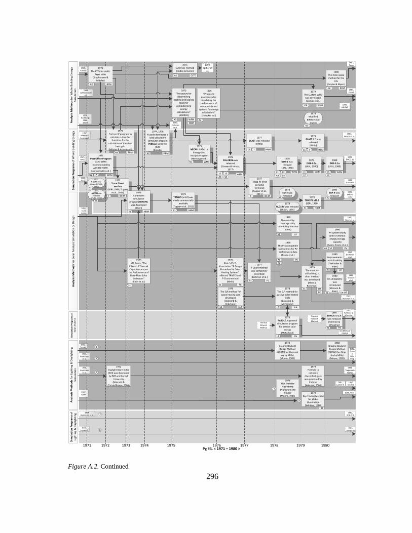
296

1975“Procedure for

determining heating and cooling

loads for computerizing

energy calculations”

(ASHRAE)

A3

N2

Sim

ula

tio

n P

rogr

ams

of

Wh

ole

Bu

ildin

g En

erg

yA

nal

ysis

Me

tho

ds

for

Wh

ole

Bu

ildin

g En

erg

y Si

mu

lati

on

Sim

ula

tio

n P

rogr

ams

of

Sola

r A

nal

ysis

An

alys

is M

eth

od

s fo

r So

lar

An

alys

is S

imu

lati

on

or

De

sign

Sim

ula

tio

n P

rogr

ams

of

Ligh

tin

g &

Day

ligh

tin

gA

nal

ysis

Me

tho

ds

for

Ligh

tin

g &

Day

ligh

tin

g Si

mu

lati

on

1974, 1976Kusuda developed a

load calculation computer program (NBSLD) using the

HBM(Kusuda)

1975NECAP, NASA＇s

Energy-Cost Analysis Program(Henninger ed.)

1979BLAST 2.0 was

released(Hittle)

1976CAL-ERDA was

released(Graven & Hirsch,

1977)

1977BLAST was released

(Hittle)

1977Trace 77 (first

personal terminal)

(Tupper et al., 2011)

N2

N1

C1

T

1978Flux Transfer Algorithms

By DiLaura and Hauser

(Moore, 1985)

1979Formula to calculate

discomfort glare was proposed by

Einhorn(Wienold, 2006)

1978Graphic Daylight Design Method

(GDDM) for Overcast sky by Millet

(Moore, 1985)

1979Ray Tracing Method

for global illumination

(Whitted, 1980)

1977F-Chart method was completely

described (Beckman et al.)

1978The monthly-average daily

utilizability function(Klein)

1978TRNSYS compatible subroutines for PV performance data

(Evans et al.) 1980Improvements to Utilizability(Theilacker &

Klein)

1980Un-utilizability

was introduced(Monsen &

Klein)1978

The SLR method for passive solar heated

walls(Balcomb & McFarland)

1976Klein’s Ph.D.

dissertation "A Design Procedure for Solar Heating Systems"

affected TRNSYS and F-Chart method

(Klein)

1976The SLR method for space heating was

developed(Balcomb & Hedstrom)

S1

S1

S1

L2

S1

A5

L2

S1

S1

1978PASOLE, A general

simulation program for passive solar

energy(McFarland)

L2

1971 1973 1975 1976 1978 1980

1980Graphic Daylight Design Method

(GDDM) for Clear sky by Millet

(Moore, 1985)

19791977

1978DOE-1 was

released(LASL, 1980)

L1

1979DOE-2.0a

(LASL, 1980)

L1

1974

1972Daylight Glare Index (DGI) was developed by BRS and Cornell

University(Wienold &

Christoffersen, 2006)

1972

1971The CTFs for multi-

layer slabs(Stephenson &

Mitalas)

1975TRNSYS (v 6.0) was made commercially

available(Tupper et al., 2011)

S1

A5

Pg #4. < 1971 – 1980 >

1973MS thesis, “The

Effects of Thermal Capacitance upon

the Performance of Flate-Plate Solar

Collectors”(Klein et al.)

1972Fortran IV program to

calculate z-transfer functions for the

calculation of transient heat gain

(Mitalas & Arseneault)N3

1971Post Office Program

used WFM recommended by

ASHRAE TGER.(Lokmanhekim ed. )

G2

HBM

WFM

HBM HBMI C1 I

WFM

HBM

RFM

WFM

RFM

WFM

WFMWFM WFM

1969, Lokmanhekim

ed.

1969, Kusuda

1967, Mitalas &

Arseneault

1967, APEC

1963, Liu &

Jordan

1969, Turner

1966, Hopkinson

et al.

1958, Hopkinson

et al.

1970, Lumen-II

1981, Kerrisk

1990, ASHRAE

1981, Herron et al.

1989, Trane 600

1981, Siegel et al.

1981, Monsen

et al.

1982, Beckman et al.

1982, Bryan

& Cals-berg

1983, Tregenza &

Walter

1986, Arvo

1982, Modest

1982, DOE-2.1b

1981, Lumen- III

1981, Lumen III

1954, Hopkinson et al.

RT

Un-UT

UT

UT

1982, Beckman

et al.

SLR

TN

L2

A4L1 L2

A4

1

2

4

5

5

1978BLDSIM was released

(Shavit, 1995)

1978ESP-I was released

1980ESP-II was released

1993, TRNSYS v14.2

1980SUNCAT v 2.4 was released(Palmiter & Wheeling)

SLR Method/PASOLE

1983, Palmiter & Wheeling

1979Modified

BIN Method(Cane)

6

7

1980The state space method for the

RFs(Ceylan & Myers)

1979The Custom WFM

was developed.(Cumali et al.)

HBM

RFMW

1979The monthly utilizability, f-chart method

was developed (Klein &

Beckman)FC

FC

WFMC4

C4

FC

UT

PV

C4 L2

1980DOE-2.1a

(LASL, 1980)

L1 WFML2

1982, DOE-2.1b

1993, Spitler et

al.

A3

1975“Proposed

procedures for simulating the

performance of components and

systems for energy calculations”(Stoecker ed.)

A1 CLTD

1975CLTD/CLF method (Rudoy & Duran)

1997, Pedersen

et al.

TNE1

S1

A2A2

1971E-CUBE was

released (PNNL, 1990)G3

1971AXCESS was

released(PNNL, 1990)

E3

1972Trace Direct

version(SERI, 1980; Tupper

et al., 2011)

T WFM

1967, GATE

N3

1973A transient simulation

program(TRNSYS) was developed

(Klein)

S1 HBM

SLR

1979TRNSYS v10.1(SERI, 1980)

S1 HBM

S2

PVS2

1967, Appel

P

1958, Buchberg;

1960, Obert

1987, Seem

Thermal Network Method

Thermal Network Method

1980PV system study with or without energy storage

capacity(Evans; Evans et al.)

Figure A.2. Continued

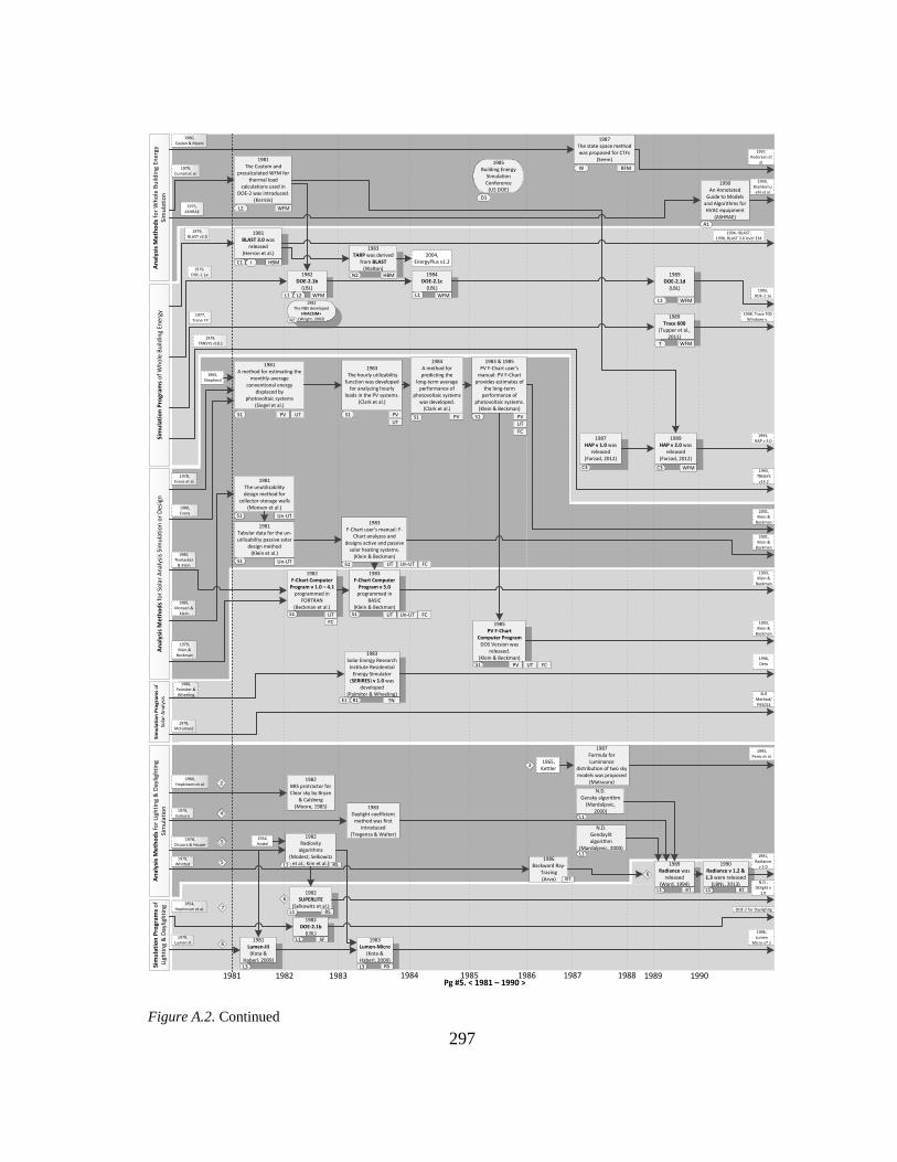
297

Sim

ula

tio

n P

rogr

am

s o

f W

ho

le B

uild

ing

Ene

rgy

An

aly

sis

Me

tho

ds

for

Wh

ole

Bu

ildin

g En

erg

y Si

mu

lati

on

Sim

ula

tio

n P

rogr

am

s o

f So

lar

An

alys

isA

na

lysi

s M

eth

od

s fo

r So

lar

An

alys

is S

imu

lati

on

or

De

sign

Sim

ula

tio

n P

rogr

am

s o

f Li

ghti

ng

& D

aylig

hti

ng

An

aly

sis

Me

tho

ds

for

Ligh

tin

g &

Day

ligh

tin

g Si

mu

lati

on

1981 1982 1984 1986 1988 1990

1984DOE-2.1c

(LBL)

1989DOE-2.1d

(LBL)

1982F-Chart Computer

Program v 1.0 – 4.1 programmed in

FORTRAN(Beckman et al.)

1983F-Chart Computer

Program v 5.0programmed in

BASIC(Klein & Beckman)

1983 The hourly utilizability

function was developed for analyzing hourly

loads in the PV systems.(Clark et al.)

1984A method for predicting the

long-term average performance of

photovoltaic systems was developed.

(Clark et al.)

1983 & 1985PV F-Chart user's

manual: PV F-Chart provides estimates of

the long-term performance of

photovoltaic systems.(Klein & Beckman)

1985PV F-Chart

Computer Program DOS Version was

released.(Klein & Beckman)

1981BLAST 3.0 was

released(Herron et al.)

1983Solar Energy Research Institute Residential

Energy Simulator (SERIRES) v 1.0 was

developed(Palmiter & Wheeling)

1989Trace 600

(Tupper et al., 2011)

C1

L1L1

T

S1

R1

S1S1

S1

S1

S1

1983Daylight coefficient

method was first introduced

(Tregenza & Walter)

1981Lumen-III(Kota &

Haberl, 2009)

1983Lumen-Micro

(Kota & Haberl, 2009)

N.D.Gensky algorithm

(Mardaljevic, 2000)

N.D.Gendaylit algorithm

(Mardaljevic, 2000)

1982SUPERLITE

(Selkowitz et al.)

1982Radiosity

algorithms(Modest; Selkowitz

et al.; Kim et al.)

1982BRS protractor for Clear sky by Bryan

& Calsberg(Moore, 1985)

1982DOE-2.1b

(LBL)

1986Backward Ray-

Tracing(Arvo)

L1

L1

L1

1981A method for estimating the

monthly-average conventional energy

displaced byphotovoltaic systems

(Siegel et al.)

1981The unutilizability design method for

collector-storage walls(Monsen et al.)

1981Tabular data for the un-utilizability passive solar

design method(Klein et al.)

S1

S1

S1

1982DOE-2.1b

(LBL)

L1

1983 1985 1987 1989Pg #5. < 1981 – 1990 >

1989Radiance was

released(Ward, 1994)

L1

HBMI

WFM WFMWFM

WFM

A1

1990An Annotated

Guide to Models and Algorithms for HVAC equipment

(ASHRAE)

1981The Custom and

precalculated WFM for thermal load

calculations used in DOE-2 was introduced.

(Kerrisk)

WFML2

1979, Cumali et al.

1975, ASHRAE

1979, BLAST v2.0

1979, DOE-2.1a

1979, TRNSYS v10.1

1978,Evans et al.

1980, Evans

1980, Monsen &

Klein

1979, Klein &

Beckman

1978, McFarland

1966, Hopkinson et al.

1979, Einhorn

1978, DiLaura & Hauser

1979, Whitted

1954, Hopkinson et al.

1970, Lumen-II

1997, Pedersen et

al.

1993, Brandemu-ehl et al.

1987HAP v 1.0 was

released(Farzad, 2012)

1990Radiance v 1.2 & 1.3 were released

(LBNL, 2013)L1

1993, DOE-2.1e

1998, Trace 700 Windows v.

1977, Trane 77

1993, HAP v 3.0

C3

1989HAP v 2.0 was

released(Farzad, 2012)

C3 WFM1993,

TRNSYS v14.2

1993, Klein &

Backman

1993, Klein &

Backman

1996, Deru

SLR Method/PASOLE

1991, Radiance

v 2.0

N.D., DElight v

1.0

DOE-2 for Daylightig

1996, Lumen

Micro v7.1

1983F-Chart user's manual: F-

Chart analyzes and designs active and passive

solar heating systems.(Klein & Beckman)

L3 L3 RS

SF

RS

RS

RT

RT RT

Un-UT

Un-UT Un-UTUTS1

1980, Theilacker

& Klein

UT Un-UTUT

PV PV PV

UT

2001, Klein &

Backman

2001, Klein &

Backman

1987Formula for Luminance

distribution of two sky models was proposed

(Matsuura)

1965, Kettler

1993, Perez et al.

2

4

5

5

3

1982The NBS developed

HVACSIM+(Wright, 2003)

1980, Palmiter & Wheeling

L17

6

6

6

1987The state space method was proposed for CTFs

(Seem)

RFMW

UT

FC

FC

L2

1994, IBLAST; 1998, BLAST 3.0 level 334

TNE1

PV

N2

1985Building Energy

Simulation Conference

(US DOE)

D1

PV UT

1965, Shepherd

1954, Hottel

L1

1983TARP was derived

from BLAST(Walton)

N2 HBM

2004, EnergyPlus v1.2

1980, Ceylan & Myers

UT

FC

FC

FC

Figure A.2. Continued

298

Sim

ula

tio

n P

rogr

ams

of

Wh

ole

Bu

ildin

g En

erg

yA

nal

ysis

Me

tho

ds

for

Wh

ole

B

uild

ing

Ene

rgy

Sim

ula

tio

nSi

mu

lati

on

Pro

gram

s o

f So

lar

An

alys

isA

nal

ysis

Me

tho

ds

for

Sola

r A

nal

ysis

Sim

ula

tio

n

Sim

ula

tio

n P

rogr

ams

of

Ligh

tin

g &

D

aylig

hti

ng

An

alys

is M

eth

od

s fo

r Li

ghti

ng

&

Day

ligh

tin

g Si

mu

lati

on

1991 1992 1994 1996 1998 20001993 1995 1997 1999

1993DOE-2.1e

(LBL)

2000DOE-2.1e-

107(LBNL)

1996EnergyPlus

development began(Crawley et al.,

1997)

1998The new generation energy simulation, EnergyPlus Alpha

Version (Crawley et al., 1999)

1999EnergyPlus Beta

Testing began(Crawley et al.,)

1996PowerDOE v1.0

/DOE-2.2(Tupper et al., 2011)

2000eQUEST v1.2

/DOE-2.2(Tupper et al., 2011)

1999eQUEST v1.0

/DOE-2.2(Tupper et al.,

2011)

1993 TRNSYS v14.2 was

released in Windows(Tupper et al., 2011)

1993F-Chart Computer Program v 6.17W programmed in

Windows(Klein & Beckman)

1993PV F-Chart Computer

Program v 3.01WWindows Version was

released.(Klein & Beckman) 1996

The upgrade of SERIRES to SUNREL

was completed(Deru)

1995DOE-2.1e-087

(LBNL)

1998Trace 700

(first Windows v.) (Tupper et al., 2011)

1999HAP v 4.0 included

a MS Windows-based GUI

(Carrier, 2013)

L1 L1

L1

D1 D2

L1

JJ

T

C3

S1

S1

S1

R1

1998DAYSIM was developed

by Reinhart’s coordination

(Reinhart, 2013)

N.D.Lumen-

Micro 2000(LT website)

Pg #6. < 1991 – 2000 >

1997EnergyBase,

combined the best features of BLAST and DOE-2 (Crawley et al.)

L1 I C1

WFM

HBMHBM

HBM

WFM

WFM

WFM

WFM

WFM

WFM

WFM

L1 I C1 HBM L1 I C1 HBM

A1 HBMWFM

1998BLAST 3.0 Level 334

was released(Crawley, 2005)

C1 HBMI

1993A Toolkit Algorithms and

Subroutines for Secondary HVAC Energy Calculations

(Brandemuehl et al.)

1999A Toolkit for Primary HVAC System Energy

Calculation(ASHRAE)

1996Annotated Guide to

Load Calculation Models and Algorithms

(Spitler)

A1A1

1991Radiance v2.0 was released (LBNL, 2013)

1992Radiance v2.1 was released (LBNL, 2013)

1993Radiance v 2.3 was released (LBNL, 2013)

1994Radiance v 2.4 was released (LBNL, 2013)

1995Radiance v 2.5 was released (LBNL, 2013)

1996Radiance v 3.0 was released (LBNL, 2013)

1997Radiance v 3.1 was released (LBNL, 2013)

1993HAP v 3.0 was

released(Farzad, 2012)

C3 WFM

1987, Seem

1990, ASHRAE

1981, BLAST v3.0

1989, DOE-2.1d

1989,Trace 600

1989, HAP v 2.0

1979, TRNSYS v10.1

1983, Klein &

Backman

1985, Klein &

Backman

1983, Palmiter & Wheeling

1978, McFarland

1990, Radiance v 1.2 & 1.3

1982, SUPERLITE

1982, DOE-2.1b

1983, Lumen Micro

2006, Trace 700

v6.0

2002, Pedersen

et al.

2001, EnergyPlus

First v.

2001, DOE-

2.1e-113

2001, eQUEST v2.17c

2001, Trace 700

2002,HAP v4.1

2001, TRNSYS v15.0

2001, Klein &

Beckman

2001,Klein &

Beckman

2002, Deru et al.

SLR Method/PASOLE

2003, DAYSIM v1.3

2002, Radiance

v3.4

N.D., DElight

v1.0

N.D.,Lumen

Designer

DOE-2 for Daylighting

N3

C5

L1 RT L1 RTL1 RT L1 RT L1 RT L1 RTL1 RT

RT

L3 RS

TN

UT Un-UT

UT

1983 & 1985,

Klein & Backman

1983, Klein &

Backman

2001, Klein & Backman

2001, Klein &

Backman

1993All weather sky

models were proposed

(Perez et al.)

1987, Matsuura 3

1994IBLAST

was released(Sowell & Hittle,

1995)

I HBM

E2

6

7

6

6

6

TRACE 700

1975, Rudoy &

Duran

A1 CLTD

1993CLTD/SCL/CLF

method (Spitler et al.)

1997The Current HBM

was organized (Pedersen et al.)

A1 HBM

1997Radiant Time Series

(RTS) Method (Spitler et al.)

A1 RTS

TRACE 700

PV

O G2 F2 O G2 F2 O G2 F2

H2 M1 F3

1996Lumen Micro v 7.1

(Ubbelohde & Humann, 1998)

1998Lumen Micro v 7.5

(Ubbelohde & Humann, 1998)

L3 RS L3 RS

FC

FC

Figure A.2. Continued

299

2001 2002 2004 2006 2008 2010

Sim

ula

tio

n P

rogr

ams

of

Wh

ole

Bu

ildin

g En

erg

yA

nal

ysis

Me

tho

ds

for

Wh

ole

B

uild

ing

Ene

rgy

Sim

ula

tio

nSi

mu

lati

on

Pro

gram

s o

f So

lar

An

alys

isA

nal

ysis

Me

tho

ds

for

Sola

r A

nal

ysis

Si

mu

lati

on

orD

esi

gnSi

mu

lati

on

Pro

gram

s o

f Li

ghti

ng

& D

aylig

hti

ng

An

alys

is M

eth

od

s fo

r Li

ghti

ng

& D

aylig

hti

ng

Sim

ula

tio

n

2003 2005 2007 2009

2002DOE-2.1e-119

(LBNL)

2001DOE-2.1e-113

(LBNL)

2003DOE-2.1e-121

(LBNL)

2001eQUEST v2.17c

/DOE-2.2(Tupper et al.,

2011)

2007eQUEST v3.6

/DOE-2.2(Tupper et al.,

2011)

2010eQUEST v3.64

/DOE-2.2(Tupper et al.,

2011)

2010EnergyPlus

v6.0 was released

(EERE, 2010)

2010TRNSYS v 17 was released(SEL website)

2002SUNREL was

registered publically

(Deru et al.)

2004SUNREL v1.14(Crawley et al.,

2005)

2004EnergyPlus v1.2

provied an option of TARP to calculate surface convection

(EERE, n.d.)

2007EnergyPlus v2.0

& v2.1(EERE, n.d.)

2009EnergyPlus v3.1

& v4.0(EERE, n.d.)

2004 TRNSYS v16 was

released

2001EnergyPlus

First Release(Crawley et al.,

2002)

2001 TRNSYS v15 was released

2001Trace 700

(full version) (Tupper et al.,

2011)

2008Trace 700 v 6.2

was released(Trane, 2013)

2006HAP v 4.3 was

released(Carrier, 2013)

2002HAP v 4.1 was

released(Carrier, 2013)

2008HAP v 4.4 was

released(Carrier, 2013)

2010HAP v 4.5

was released(Carrier,

2013)

2003HAP v 4.2 was

released(Carrier, 2013)

2006Trace 700 v 6.0

was released(Trane, 2013)

2005Daylight

Autonomy (DA)(Nabil &

Mardaljevic, 2006)

2006Useful Daylight

Illuminances (UDI)(Nabil &

Mardaljevic)

N.D.DElight v1.0

2004DElight v2 full

integration with EnergyPlus v1.2

(EERE., n.d.)

N.D.DElight v2.0

N.D.Lumen

Designer(LT website)

J

L1

T

S1

J

L1

C3C3

J

L1

S1

R1 R1

T

C3 C3

T

S1

C3

Pg #7. < 2001 – 2010 >

L1

2006EnergyPlus v1.3

& v1.4(EERE, n.d.)

2008EnergyPlus v2.2

& v3.0(EERE, n.d.)

2003EnergyPlus v1.1

was released (EERE, n.d.)

2005eQUEST v3.55

/DOE-2.2(JJH website)

J

WFMWFM WFM

RTSRTS

HBMHBM HBM

WFMWFM WFM

WFM

WFM

WFM

WFM

HBM

L1 I HBML1 I HBM

L1 I C1

HBML1 I HBM

L1 I HBM L1 I HBM L1 I HBM L1 I HBM

WFM

WFMWFM WFM WFM

2002ASHRAE Toolkit for

Building Load Calculations

(Pedersen et al.)

A1

1997, Spitler et

al.

1999, ASHRAE

1999, EnergyPlus

Beta

2000, DOE-2.1e-107

2000, eQUEST

v1.2

1998, Trace 700

Windows v.

1999, HAP v4.0

1996,TRNSYS v14.2

1996, Deru

1978, McFarland

1998, DAYSIM

1997, Radiance

v3.1

1982, SUPERLITE

N.D., Lumen-Micro

2000

2011, EP

v7.0

2002Trace 700 v 4.1

was released(Trane, 2013)

T WFM

2002Radiance v3.4(LBNL, 2013)

L1 RT

2003Radiance v3.5(LBNL, 2013)

L1 RT

2005Radiance v3.7(LBNL, 2013)

L1 RT

2008Radiance v3.9(LBNL, 2013)

L1 RT

2002DAYSIM v1.3

(Reinhart, 2013)N3 RT

2003DAYSIM v2.0

(Reinhart, 2013)RT

2005DAYSIM v2.1

(Reinhart, 2013)RT

2010DAYSIM v3.X was released

(Reinhart, 2012) RT

DOE-2.1e

eQUEST

2012, Trace 700 v6.2.9

2012, HAP v4.6

& 4.61

2012, TRNSYS v17.1

2013, DAYSIM

v4.0

2011, Radiance

v4.1

DOE-2 for Daylighting

Lumen Micro

F-Chart Computer Program

PV F-Chart Computer Program

SUNREL

SLR Method/PASOLE

2010Radiance v4.0 (LBNL, 2013)

L1 RTEnergyPlus for Daylighting

RS

TNTN

2001PV F-Chart user's manual

(Klein & Beckman) UT

2001F-Chart user's manual

(Klein & Beckman)S1 UT

2001F-Chart

Windows v.(Klein &

Beckman)

2001PV F-Chart

Windows v. (Klein &

Beckman)S1

S1 UT Un-UT

UT

Un-UT

1993, PV F-Chart Windows v.

1993, F-Chart

Windows v.

S1

6

6

7

6

6

7

PV

O G2 F2

2003eQUEST v3.40

/DOE-2.2(JJH website)

J WFM

1983, TARP

H2M1 F3

N3

H2M1 F3 N3 H2M1 F3 N3 H2M1 F3

1982, DOE-2.1b

L3 RS

PV FC

FC

FC

FC

L1 RSL1 RS

Figure A.2. Continued

300

Radiance

eQUEST/DOE-2.2

DOE-2.1e

EnergyPlus

TRNSYS

TRACE

HAP

2011 2012

Sim

ulat

ion

Prog

ram

s of

Who

le B

uild

ing

Ener

gyA

naly

sis

Met

hods

for

Who

le

Build

ing

Ener

gy S

imul

atio

nSi

mul

atio

n Pr

ogra

ms

of S

olar

Ana

lysi

sSi

mul

atio

n Pr

ogra

ms

of L

ight

ing

& D

aylig

htin

gA

naly

sis

Met

hods

for

Ligh

ting

& D

aylig

htin

g Si

mul

atio

n

F-Chart Computer Program

PV F-Chart Computer Program

SLR method/PASOLE

Lighting & Daylighting

Analysis Simulation

EnergyPlus for Daylighting

WholeBuilding Energy

Simulation

Pg #8. < 2011 – Present >

SUNREL

Daysim

DOE-2 for Daylighting

Solar Thermal Simulation

2011EnergyPlus v7.0

was released(EERE, 2011e)

2012EnergyPlus v7.1

and v7.2 was released

(EERE, 2012)

Lumen Micro

Ana

lysi

s M

etho

ds

for

Sola

r A

naly

sis

Sim

ulat

ion

orD

esig

n

Solar PV Simulation

Passive Solar Simulation

WFM

L1 I HBML1 I HBM L1 I HBM

L1 WFM

J

T RTSWFM

C3 WFM

S1 HBM

2012Trace 700 v 6.2.9

was released(Trane, 2013)

T RTSWFM

2012HAP v 4.6 & 4.61

were released(Carrier, 2013)

C3 WFM

2012TRNSYS v 17.1 was released(SEL website)

S1 HBM

S1

S1

R1

L2

UT

UT

TN

TN

RT

L1 RT

L1 RS

L1 SF

L3 RS

SF

2011Radiance v4.1(LBNL, 2013)

L1 RT

2010, EP

v6.0

2003, DOE-2.1e-

121

2010, eQUEST

v3.64

2008, Trace

700 v6.2

2010, HAP v4.5

2010, TRNSYS v17.0

2010, DAYSIM

v3.X

2010, Radiance

v4.0

2004, DElight

v2.0

N.D.,Lumen

Designer

2001, F-Chart

Windows v.

2001, PV F-Chart Windows v.

2004, SUNREL

v1.14

1978, McFarland

Un-UT

6

7

7

6

TT CLTD

Solar System Simulation or

Design

SLR

PV

2013

2013EnergyPlus v8.0

was released(EERE, 2013b)

L1 I HBM

N3 H2M1 F3

2013DAYSIM v4.0

(Reinhart, 2013)N3 H2M1 F3 6RT

1982, DOE-2.1b

FC

FC

Figure A.2. Continued

301

APPENDIX B

Table B.1. Annotated references of the analysis methods of the whole-building energy simulation programs.

Sorter Year Author Who were they? Literature Title What did the literature do? Why was it important?

Time

Equivalent

Tempera-ture

Difference

(TETD)/ Time

Averaging

(TA) Method

1935

Faust, F.,

Levine,

L., & Urban, F.

Engineers at the General Electric

Corporation

A rational heat gain

method for the determination of air

conditioning cooling

loads

Faust et al. calculated the cooling load using

a time lag effect of walls.

The time lag accounted for the effect of

wall’s thermal storage capacity. In other

words, the time lag concept accounted for time delay and heat amplitude reduction

between an outer surface and an inter surface

of a wall (Faust et al., 1935; Alford et al., 1939).

1939

Alford, J., Ryan, J.,

& Urban,

F.

Engineers at the

General Electric Corporation

Effect of heat storage

and variation in outdoor temperature

and solar intensity on

heat transfer through walls

Alford et al. proposed a decrement factor to

visualize the wall’s thermal storage capacity.

The concept of a decrement factor was used

for Mackey and Wright’s study (Mackey and Wright, 1944).

1944

Mackey,

C. O. &

Wright, L. T.

Professors at Cornell

University

Periodic heat flow – homogeneous walls or

roofs.

Mackey and Wright’s study assumed

periodic cycles of steady state temperature on

a one-day basis for calculating heat gain through walls and roofs (Kusuda, 1969).

They employed Fourier series rather than the

Laplace transform to calculate heat conduction equations due to the low speed of

computers (Mackey and Wright, 1944;

Kusuda, 1969).

1946

Mackey,

C. O. &

Wright, L. T.

Professors at Cornell

University

Periodic heat flow – composite walls or

roofs.

Previous study was extended to composite

walls.

This study contributed to the development of

the ETD method.

1948 Stewart, J. Engineer at the

Carrier Corporation

Solar heat gain

through walls and

roofs for cooling load calculations

The ETD method (later the TETD method) was outlined and tabled for calculating heat

gain of practical walls.

This study contributed to the development of

the TETD method.

1961 ASHRAE ASHRAE ASHRAE Guide and

Data Book

The TETD/TA method using the TA was

introduced to calculate cooling load.

Even though the TETD/TA was developed as

a manual method at first, this method has

also been used as a computer procedure

(McQuiston and Spitler, 1992). For example,

the HCC program developed by APEC in

1967 used the TETD/TA method (Ayres and Stamper, 1995).

302

Table B.1. Continued

Sorter Year Author Who were they? Literature Title What did the literature do? Why was it important?

Response

Factor Method

(RFM)/

Conduction Transfer

Function

(CTF) Method

1925

Nessi, A.

& Nisolle, L.

Engineers, Ėcole

Centrale Paris (French University)

Regimes variables de

fonctionnement dans

les installations de chauffage central

(Regime variables of

operation in the installations of central

heating)

Nessi and Nisolle employed the superposition of unit step functions rather

than triangular pulses (Stephenson, D. G. &

Mitalas, G. P., 1967).

The response factor method of calculating

transient heat flow was used first (Stephenson, D. G. & Mitalas, G. P., 1967).

1947 Tustin, A.

British engineer,

professor of engineering at the

University of

Birmingham

A method of analyzing

the behavior of linear

systems in terms of time series

Prof. Tustin showed that time-series are very similar to polynomials in that they can be

added, subtracted, multiplied and divided.

The commutative and distributive laws of ordinary arithmetic also apply for time-series

(Stephenson, D. G. & Mitalas, G. P., 1967).

The concept of a time-series was first presented by Tustin, in 1947 (Stephenson, D.

G. & Mitalas, G. P., 1967).

1956

Brisken,

W. R. & Reque, S.

G.

Manager, commercial and industrial air

conditioning department, General

Electric Co. /

Systems analysis engineer, electrical

engineering

laboratory, GE Co.

Heat load calculations by thermal response

Steady-state load factors were modified to

include transient effects and special allowances were recommended for internal

heat storages of the buildngs. This procedure,

the thermal response method was further developed in this study (Brisken, W. R. &

Reque, S. G.).

Unique features of the thermal response method were found in this study. However,

the response factors due to rectangular pulses

were still used (Stephenson, D. G. & Mitalas, G. P., 1967).

1957 Hill, P. R.

Researcher, National

Advisory Committee

for Aeronautics (NACA)

A method of

computing the transient temperature

of thick walls from

arbitrary variation of adiabatic-wall

temperature and heat-

transfer coefficient

Formulas to facilitate the determination of the transient surface temperatures of thick

walls from an arbitrary variation of adiabatic-

wall temperature and heat-transfer coefficient have been developed. Formulas to facilitate

the determination of heat flow from an

arbitrary variation of wall surface temperature were also obtained (Hill, P. R.,

1957).

A simple method is developed for the calculation of the temperature history of the

surfaces of a thick wall or of any plane

within the wall (Hill, P. R., 1957). The first application of triangular pulses was used

(Stephenson, D. G. & Mitalas, G. P., 1967).

303

Table B.1. Continued

Sorter Year Author Who were they? Literature Title What did the literature do? Why was it important?

Response Factor

Method

(RFM)/ Conduction

Transfer

Function

(CTF)

Method

1967 Mitalas, G. P. & Stephenson,

D. G.

Researchers,

Building Services

Section, Division of Building

Research, National

Research Council, Canada

Room thermal

response factors

Room thermal response factors were developed for improving previous response

factors of Brisken and Reque.

This paper presented a method of computing the factors for any room. It differs from the

earlier work by Brisken and Reque.

1967

Mitalas, G. P.

& Arseneault, J. G.

Researchers,

Division of Building

Research, National

Research Council, Canada

Fortran IV program to calculate heat flux

response factors for a

multi-layer slab

Mitalas and J. G. Arseneault developed a FORTRAN IV program to calculate heat gain

through multi-layered slabs using the RFM of

Mitalas and Stephenson.

This Laplace transform approach was able to

improve the calculation accuracy by the lumped RC approach of Brisken and Reque.

1971 Stephenson,

D. G.&

Mitalas, G. P.

Researchers,

Building Services

Section, Division of Building

Research, National

Research Council, Canada

Calculation of heat

conduction transfer

functions for multi-layer slabs

CTFs use a heat flux history in place of a temperature history using the z-transform

functions.

The computer procedure for calculating

instantaneous heat gain using CTFs is more efficient than the procedure using RFs

because it calculates faster and uses less

memory space.

1971 Lokmanhekim

ed.

ASHRAE Task

Group on Energy

Requirements (TGER)

Procedure for

determining heating

and cooling loads for

computerized energy

calculations – algorithms for

building heat transfer

subrouties.

ASHRAE TGER adopted the RFM that uses CTFs. This booklet shows the computer

algorithms for the RFM.

These publications helped researchers and

engineers quickly learn the basic knowledge

of whole-building simulation programs,

which accelerated the development of whole-building energy simulation (Sowell and

Hittle, 1995).

1980 Ceylan, H. &

Myers, G.

Graduate student

and professor at

the University of Wisconsin-

Madison

Long-time solutions to heat-conduction

transients with time

dependent inputs

They compared the state space method with

other solution procedures (UIUC and LBNL, 2012).

Without applying z-transform, this study

suggested a method to calculate response factors.

1987 Seem, J. E.

Graduate student at the University

of Wisconsin-

Madison

Modeling of heat

transfer in buildings

Seem shows the procedures to calculate the

CTFs using the state space method.

This study showed the state space method reduced the calculation time to estimate the

CTFs rather than the Laplace transform

approach.

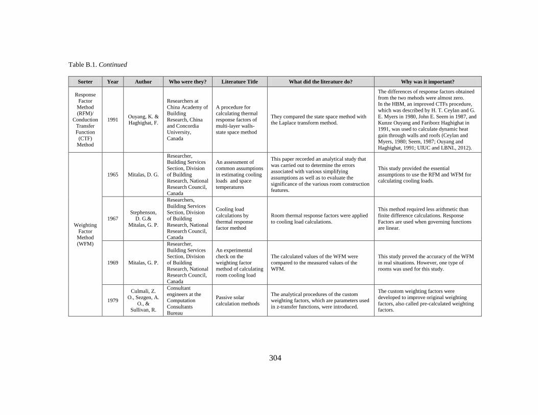
304

Table B.1. Continued

Sorter Year Author Who were they? Literature Title What did the literature do? Why was it important?

Response

Factor

Method (RFM)/

Conduction

Transfer Function

(CTF)

Method

1991 Ouyang, K. & Haghighat, F.

Researchers at

China Academy of Building

Research, China

and Concordia University,

Canada

A procedure for calculating thermal

response factors of

multi-layer walls-state space method

They compared the state space method with the Laplace transform method.

The differences of response factors obtained

from the two mehods were almost zero. In the HBM, an improved CTFs procedure,

which was described by H. T. Ceylan and G.

E. Myers in 1980, John E. Seem in 1987, and Kunze Ouyang and Fariborz Haghighat in

1991, was used to calculate dynamic heat

gain through walls and roofs (Ceylan and Myers, 1980; Seem, 1987; Ouyang and

Haghighat, 1991; UIUC and LBNL, 2012).

Weighting

Factor Method

(WFM)

1965 Mitalas, D. G.

Researcher, Building Services

Section, Division

of Building Research, National

Research Council,

Canada

An assessment of

common assumptions

in estimating cooling loads and space

temperatures

This paper recorded an analytical study that

was carried out to determine the errors associated with various simplifying

assumptions as well as to evaluate the

significance of the various room construction features.

This study provided the essential

assumptions to use the RFM and WFM for calculating cooling loads.

1967 Stephenson,

D. G.&

Mitalas, G. P.

Researchers,

Building Services

Section, Division of Building

Research, National

Research Council, Canada

Cooling load

calculations by

thermal response

factor method

Room thermal response factors were applied

to cooling load calculations.

This method required less arithmetic than

finite difference calculations. Response

Factors are used when governing functions

are linear.

1969 Mitalas, G. P.

Researcher,

Building Services Section, Division

of Building

Research, National Research Council,

Canada

An experimental check on the

weighting factor

method of calculating room cooling load

The calculated values of the WFM were

compared to the measured values of the

WFM.

This study proved the accuracy of the WFM

in real situations. However, one type of

rooms was used for this study.

1979

Culmali, Z.

O., Sezgen, A.

O., & Sullivan, R.

Consultant

engineers at the Computation

Consultants

Bureau

Passive solar

calculation methods

The analytical procedures of the custom weighting factors, which are parameters used

in z-transfer functions, were introduced.

The custom weighting factors were

developed to improve original weighting

factors, also called pre-calculated weighting factors.

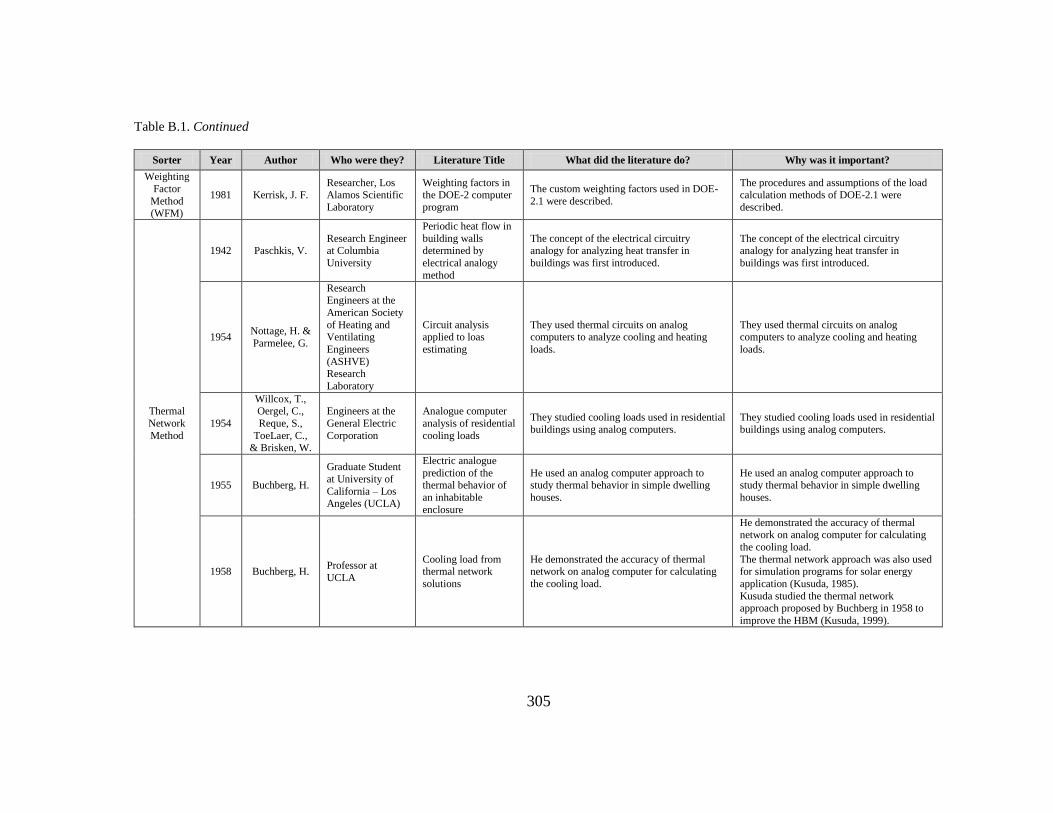
305

Table B.1. Continued

Sorter Year Author Who were they? Literature Title What did the literature do? Why was it important?

Weighting

Factor

Method (WFM)

1981 Kerrisk, J. F. Researcher, Los Alamos Scientific

Laboratory

Weighting factors in the DOE-2 computer

program

The custom weighting factors used in DOE-

2.1 were described.

The procedures and assumptions of the load calculation methods of DOE-2.1 were

described.

Thermal

Network

Method

1942 Paschkis, V. Research Engineer at Columbia

University

Periodic heat flow in

building walls determined by

electrical analogy

method

The concept of the electrical circuitry analogy for analyzing heat transfer in

buildings was first introduced.

The concept of the electrical circuitry analogy for analyzing heat transfer in

buildings was first introduced.

1954 Nottage, H. &

Parmelee, G.

Research Engineers at the

American Society

of Heating and Ventilating

Engineers

(ASHVE) Research

Laboratory

Circuit analysis applied to loas

estimating

They used thermal circuits on analog computers to analyze cooling and heating

loads.

They used thermal circuits on analog computers to analyze cooling and heating

loads.

1954

Willcox, T., Oergel, C.,

Reque, S.,

ToeLaer, C.,

& Brisken, W.

Engineers at the

General Electric

Corporation

Analogue computer

analysis of residential

cooling loads

They studied cooling loads used in residential buildings using analog computers.

They studied cooling loads used in residential buildings using analog computers.

1955 Buchberg, H.

Graduate Student

at University of

California – Los Angeles (UCLA)

Electric analogue

prediction of the thermal behavior of

an inhabitable

enclosure

He used an analog computer approach to study thermal behavior in simple dwelling

houses.

He used an analog computer approach to study thermal behavior in simple dwelling

houses.

1958 Buchberg, H. Professor at

UCLA

Cooling load from thermal network

solutions

He demonstrated the accuracy of thermal network on analog computer for calculating

the cooling load.

He demonstrated the accuracy of thermal network on analog computer for calculating

the cooling load.

The thermal network approach was also used for simulation programs for solar energy

application (Kusuda, 1985).

Kusuda studied the thermal network approach proposed by Buchberg in 1958 to

improve the HBM (Kusuda, 1999).

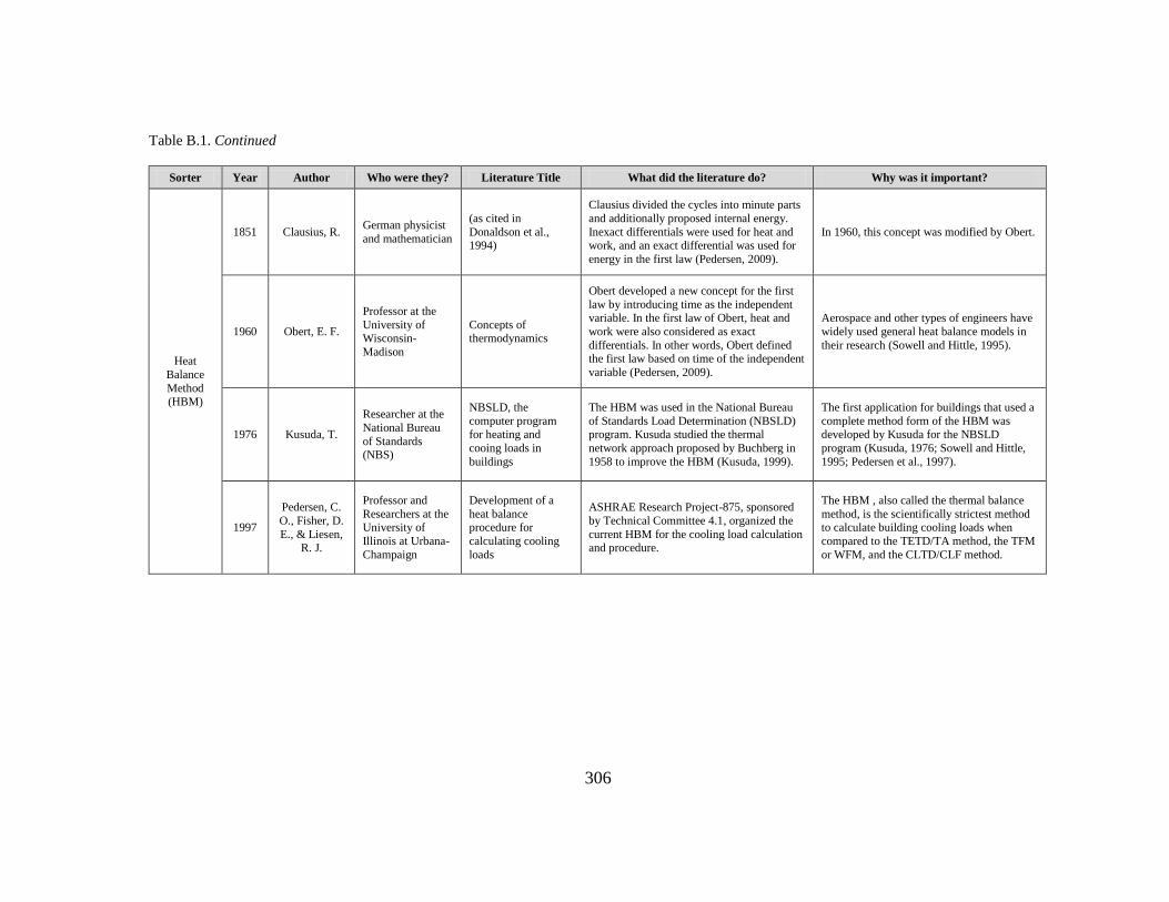
306

Table B.1. Continued

Sorter Year Author Who were they? Literature Title What did the literature do? Why was it important?

Heat

Balance

Method (HBM)

1851 Clausius, R. German physicist

and mathematician

(as cited in

Donaldson et al., 1994)

Clausius divided the cycles into minute parts

and additionally proposed internal energy.

Inexact differentials were used for heat and work, and an exact differential was used for

energy in the first law (Pedersen, 2009).

In 1960, this concept was modified by Obert.

1960 Obert, E. F.

Professor at the

University of Wisconsin-

Madison

Concepts of thermodynamics

Obert developed a new concept for the first

law by introducing time as the independent variable. In the first law of Obert, heat and

work were also considered as exact

differentials. In other words, Obert defined the first law based on time of the independent

variable (Pedersen, 2009).

Aerospace and other types of engineers have

widely used general heat balance models in

their research (Sowell and Hittle, 1995).

1976 Kusuda, T.

Researcher at the

National Bureau

of Standards (NBS)

NBSLD, the

computer program for heating and

cooing loads in

buildings

The HBM was used in the National Bureau

of Standards Load Determination (NBSLD) program. Kusuda studied the thermal

network approach proposed by Buchberg in

1958 to improve the HBM (Kusuda, 1999).

The first application for buildings that used a

complete method form of the HBM was developed by Kusuda for the NBSLD

program (Kusuda, 1976; Sowell and Hittle,

1995; Pedersen et al., 1997).

1997

Pedersen, C.

O., Fisher, D.

E., & Liesen, R. J.

Professor and

Researchers at the University of

Illinois at Urbana-

Champaign

Development of a

heat balance procedure for

calculating cooling

loads

ASHRAE Research Project-875, sponsored

by Technical Committee 4.1, organized the

current HBM for the cooling load calculation and procedure.

The HBM , also called the thermal balance

method, is the scientifically strictest method to calculate building cooling loads when

compared to the TETD/TA method, the TFM

or WFM, and the CLTD/CLF method.

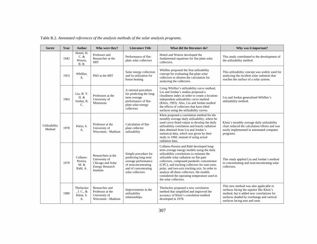
307

Table B.2. Annotated references of the analysis methods of the solar analysis programs.

Sorter Year Author Who were they? Literature Title What did the literature do? Why was it important?

Utilizability

Method

1942

Hottel, H.

C. &

Woertz, B. B.

Professor and Researcher at the

MIT

Performance of flat-

plate solar collectors

Hottel and Woertz developed the fundamental equations for flat-plate solar

collectors.

This study contributed to the development of

the utilizability method.

1953 Whillier,

A. PhD at the MIT

Solar energy collection and its utilization for

house heating

Whillier proposed the first utilizability

concept for evaluating flat-plate solar

collectors to shorten the calculation for

analyzing the collectors.

This utilizability concept was widely used for analyzing the incident solar radiation that

reaches the surface of a solar system.

1963

Liu, B. Y.

H. &

Jordan, R. C.

Professors at the University of

Minnesota

A rational procedure for predicting the long-

term average

performance of flat-plate solar-energy

collectors

Using Whillier’s utilizability curve method,

Liu and Jordan’s studies proposed a

cloudiness index in order to create a location-independent utilizability curve method

(Klein, 1993). Also, Liu and Jordan studied

the effects of collectors that have tilted surfaces using the utilizability curves.

Liu and Jordan generalized Whillier’s

utilizability method.

1978 Klein, S.

A.

Professor at the

University of

Wisconsin - Madison

Calculation of flat-

plate collector

utilizability

Klein proposed a correlation method for the

monthly average daily utilizability, where he

used curve-fitted values to develop the daily utilizability correlation and hourly radiation

data obtained from Liu and Jordan’s

statistical data, which was given by their study in 1960, instead of using actual

radiation data.

Klein’s monthly average daily utilizability chart reduced the calculation efforts and was

easily implemented in automated computer

programs.

1979

Collares-

Pereira,

M. & Rabl, A.

Researchers at the

University of Chicago and Solar

Energy Research

Institute

Simple procedure for predicting long term

average performance

of nonconcentrating and of concentrating

solar collectors

Collares-Pereira and Rabl developed long-

term average energy models using the daily

utilizability correlations to estimate the utilizable solar radiation on flat-pate

collectors, compound parabolic concentrator

(CPC), and tracking collectors for east-west, polar, and two-axis tracking axis. In order to

analyze all these collectors, the models

considered the operating temperature used in the solar collectors.

This study applied Liu and Jordan’s method to concentrating and nonconcentrating solar

collectors.

1980

Theilacker

, J. C., & Klein, S.

A.

Researcher and

Professor at the University of

Wisconsin - Madison

Improvements in the

utilizability

relationships.

Theilacker proposed a new correlation

method that simplified and improved the accuracy of Klein’s correlation method

developed in 1978.

This new method was also applicable to surfaces facing the equator like Klein’s

method, but it added new correlations for

surfaces shaded by overhangs and vertical surfaces facing east and west.

308

Table B.2. Continued

Sorter Year Author Who were they? Literature Title What did the literature do? Why was it important?

Utilizability

Method 1982

Evans, D.

L., Rule, T. T., &

Wood, B.

D.

Professors at Arizona

State University

A new look at long

term collector

performance and utilizability

Evans et al. developed a new method that

used the actual collector parameters instead

of using the critical level. This method used an empirical approach for the monthly

utilizability to analyze flat-plate collectors,

especially for tilted collectors facing south, and the collector efficiency.

This empirical approach could quickly

determine the results according to the

changes of location, design and inlet temperature of collectors.

F-Chart Method

1976 Klein, S.

A.

Professor at the

University of Wisconsin - Madison

A design procedure for

solar heating systems Klein suggested the f-chart method.

The f-chart method was further developed for customary types of active solar systems such

as active domestic hot water systems (i.e.,

two-tank domestic water heating systems), pebble bed storage space and domestic water

heating systems, and water storage space and

domestic water heating systems.

1979

Klein, S. A., &

Beckman,

W. A.

Professors at the

University of Wisconsin - Madison

A general design

method for closed-loop solar energy systems.

Klein and Beckman developed the monthly

utilizability, f-chart method.

This study extended the f-chart concept to

other applications such as concentrating solar collectors.

1979

Jurinak, J.

J., & Abdel-

Khalik, S. I.

Researcher and

Professor at the

University of Wisconsin - Madison

Sizing phase-change

energy storage units

for air-based solar heating systems

Jurinak and Abdel-Khalik performed

simulations for air-based solar heating

systems using the TRNSYS program, which led to correlations for air type systems.

In their study, a correction factor obtained

from the simulation results was then applied

to the f-chart method for estimating phase change energy storage systems.

1980

Buckles, W. E., &

Klein, S.

A.

Researcher and Professor at the

University of

Wisconsin - Madison

Analysis of solar

domestic hot water heaters

Buckles and Klein developed a modified f-

chart method.

This study analyzed domestic hot water

systems that used for a single tank system.

Originally, the f-chart method was proposed for domestic hot water systems with two tank

systems.

1980

Anderson, J. V.,

Mitchell,

J. W., & Beckman,

W. A.

Researcher and

Professors at the

University of Wisconsin - Madison

A design method for parallel solar-heat

pump systems

Anderson et al. conducted a study concerning

parallel solar heat pump systems. They used

the results of simulations to propose a design method for the systems.

This design method utilized the f-chart method to calculate the fraction of the

monthly solar energy load.

1983

Braun, J.

E., Klein, S. A., &

Pearson,

K. A.

Researchers and

Professor at the

University of Wisconsin - Madison

An improved design method for solar water

heating systems

Braun et al. developed the monthly utilizability, f-chart method for open-loop

systems.

This study expanded the monthly

utilizability, f-chart method for close-loop

solar energy systems, developed by Klein and Beckman in 1979.

309

Table B.2. Continued

Sorter Year Author Who were they? Literature Title What did the literature do? Why was it important?

F-Chart

Method 1985

Evans, B.

L., Klein,

S. A., & Duffie, J.

A.

Researcher and Professors at the

University of

Wisconsin - Madison

A design method for

active-passive hybrid space heating systems

Evans et al. performed simulations for active-

passive hybrid space heating systems using the TRNSYS program.

Their simulation results developed a new correction factor that could be applied to the

f-chart method for analyzing the hybrid

active-passive space heating systems

SLR

Method

1976

Balcomb,

J. D., &

Hedstrom,

J. C.

Researchers at Los

Alamos Scientific

Laboratory

A simplified method for calculating

required solar collector

array size for space heating

Balcomb and Hedstrom developed the SLR

method for estimating the required solar

collector array size for space heating.

The SLR method was developed to use for passive solar systems in a condition without

an active solar system. They correlated the

results from a detailed simulation program, PASOLE.

1978

Balcomb,

J. D., & McFarlan

d, R. D.

Researchers at Los

Alamos Scientific

Laboratory

A simple empirical

method for estimating

the performance of a passive solar heated

building of the thermal

storage wall type

Balcomb and McFarland proposed the SLR method for passive solar heated walls.

The SLR method was extended.

1981

Schnurr, N. M.,

Hunn, B.

D., & Williamso

n, K. D.

Researchers at Los Alamos Scientific

Laboratory

The solar load ratio

method applied to commercial building

active solar system

sizing

Schnurr et al. proposed an extension to the

SLR method.

This extended method was used for

estimating space and water heating systems

used in commercial buildings. In the use of the results from the DOE-2 detailed

simulation program, new correlations were

developed for these space and water heating

systems.

1984

Balcomb,

J. D., Jones, R.

W.,

McFarland, R.D., &

Wray, W.

O.

Researchers at Los Alamos Scientific

Laboratory

Passive solar heating analysis: a design

manual.

Balcomb et al. defined a new SLR method to

specifically analyze passive solar systems.

The SLR method of this study is the present

definition (Jones and Wray, 1992).

310

Table B.2. Continued

Sorter Year Author Who were they? Literature Title What did the literature do? Why was it important?

Un-

tilizability

Method

1980

Monsen,

W. A., &

Klein, S.A.

Researcher and

Professor at the

University of Wisconsin - Madison

Prediction of direct gain solar heating

system performance

Monsen and Klein developed the un-

utilizability method for passive solar systems.

In this method, they applied the un-utilizability concept to estimate the

performance of direct solar gain systems.

1981

Monsen,

W. A., Klein,

S.A., &

Beckman, W. A.

Researcher and Professors at the

University of

Wisconsin - Madison

The unutilizability

design method for

collector-storage walls

Monsen et al. further developed the un-

utilizability method to analyze collector-

storage walls (i.e., thermal storage walls).

The un-utilizability method was extended.

1981

Klein, S.

A.,

Monsen, W. A., &

Beckman,

W. A.

Researcher and

Professors at the University of

Wisconsin - Madison

Tabular data for the

unutilizability passive

solar design method.

Klein et al. proposed tables for simplifying the un-utilizability procedure.

The simplified approach for the un-utilizability method was proposed.

PV Design

Method

1965 Shepherd,

C. M.

Researcher at the U.

S. Naval Research Laboratory

Design of primary and secondary cells: II. An

equation describing

battery discharge

This study explained an equation for cell and

battery discharges.

Siegel et al. (1981) used the battery model of

this study.

1978

Evans, D.

L., Facinelli,

W. A., &

Otterbein, R. T.

Professors at Arizona

State University and

Researchers at the Sandia National

Laboratories

Combined

photovoltaic/thermal system studies

Evans et al. developed the TRNSYS

compatible subroutines to estimate PV performance data.

Siegel et al’s method (1981) used the

TRNSYS compatible subroutines and a 2-V battery cell model of this study.

1980 Evans, D.

L.

Professor at Arizona

State University

Simplified method for predicting photovoltaic

array output

A method for the long term, monthly average

PV array output was proposed.

Evans’s method accounted for the average

PV array output without energy storage

capacity using a computational method and graphs.

1980

Evans, D. L.,

Facinelli, W. A., &

Koehler,

L. P.

Professors at Arizona State University

Simulation and

simplified design studies of photovoltaic

systems

TRNSYS simulations were conducted to study PV systems with electrical storage.

Evans et al.’s method considered the effect of

energy storage capacity for estimating the solar load fraction of PV systems by using

graphs.

1980

Gupta, Y.,

& Young,

S.

Science Applications, Inc.

Method of predicting

long-term average performance of

photovoltaic systems.

A method for the excess array capacity was developed.

Gupta and Young predicted the excess

capacity of the array by using Liu and Jordan’s utilizabilty method developed in

1963.

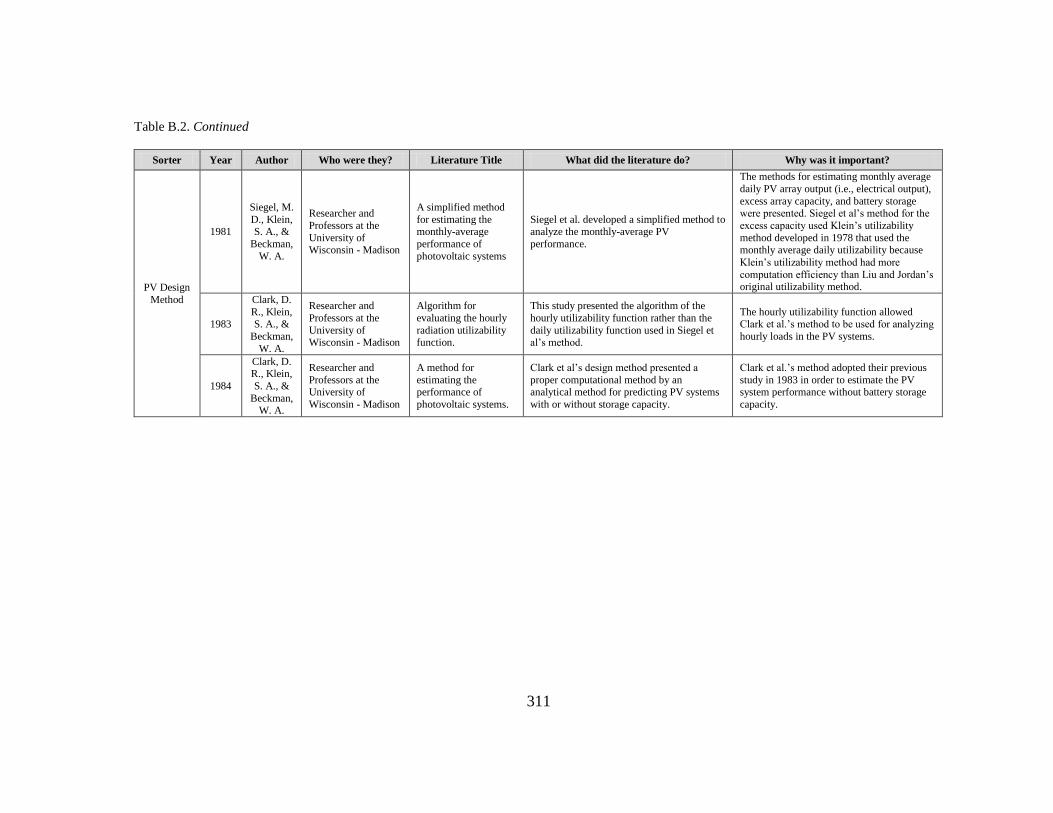
311

Table B.2. Continued

Sorter Year Author Who were they? Literature Title What did the literature do? Why was it important?

PV Design

Method

1981

Siegel, M.

D., Klein, S. A., &

Beckman,

W. A.

Researcher and

Professors at the

University of Wisconsin - Madison

A simplified method

for estimating the monthly-average

performance of

photovoltaic systems

Siegel et al. developed a simplified method to analyze the monthly-average PV

performance.

The methods for estimating monthly average

daily PV array output (i.e., electrical output),

excess array capacity, and battery storage were presented. Siegel et al’s method for the

excess capacity used Klein’s utilizability

method developed in 1978 that used the monthly average daily utilizability because

Klein’s utilizability method had more

computation efficiency than Liu and Jordan’s original utilizability method.

1983

Clark, D.

R., Klein, S. A., &

Beckman,

W. A.

Researcher and

Professors at the

University of Wisconsin - Madison

Algorithm for

evaluating the hourly

radiation utilizability function.

This study presented the algorithm of the

hourly utilizability function rather than the

daily utilizability function used in Siegel et al’s method.

The hourly utilizability function allowed Clark et al.’s method to be used for analyzing

hourly loads in the PV systems.

1984

Clark, D. R., Klein,

S. A., &

Beckman, W. A.

Researcher and

Professors at the University of

Wisconsin - Madison

A method for

estimating the performance of

photovoltaic systems.

Clark et al’s design method presented a

proper computational method by an analytical method for predicting PV systems

with or without storage capacity.

Clark et al.’s method adopted their previous

study in 1983 in order to estimate the PV system performance without battery storage

capacity.

312

Table B.3. Annotated references of the analysis methods of the lighting and daylighting analysis programs.

Sorter Year Author Who were they? Literature Title What did the literature do? Why was it important?

Split Flux

Method

1954

Hopkin-

son, R.

G., Longmore

, J., &

Pether-bridge, P.

Researchers at the Building Research

Station, UK

An empirical formula

for the computation of

the indirect component

of daylight factor

Hopkins et al. presented the split flux method

based on Arndt’s method (1954).

The split flux method was used to estimate

the IRC using an empirical formula. The split

flux method assumes interior surfaces of a room are a connected sphere shape and

perfectly diffuse with no inner obstacles, so it

works best when a room is shape as a cube and does not have internal partitions. Due to

these reasons, the internally reflected

illuminance at the back side of a room may be over-predicted when the ceiling height of

a room is much less than the depth of the

window-wall (Winkelmann and Selkowitz, 1985).

1989 Tregenza,

P. R.

Professor at the

University of Nottingham, UK

Modification of the

split-flux formulae for mean daylight factor

and internal reflected

component with large external obstructions.

Tregenza presented a modified method of the

split flux method.

Tregenza presented a modified method of the

split flux method to account for large external obstacles such as overhang.

Radiosity Method

1954 Hottel, H.

C. Professor at the MIT

Radiant-heat

transmission

Hottel first devised the radiosity method

(Siegel and Howell, 1972).

This study was the first introduction of the

radiosity method.

1966

Sparrow,

E. M., &

Cess, R. D.

Professor at the University of

Minnesota and

Professor at State University of New

York – Stony Brook

Radiation heat transfer Sparrow and Cess introduced the radiosity

concept in their book.

They described the radiosity concept in

detail.

1982 Modest,

M. F.

Professor at the

University of Southern California –

Los Angeles

A general model for

the calculation of daylighting in interior

spaces.

Modest develop the algorithm for digital

computers to calculate the daylighting effects

inside rooms in buildings.

The radiosity method was used for the algorithm.

1984

Goral, C.

M.,

Torrance, K. E.,

Greenberg

, D. P., Battaile,

B.

Professors and

graduate students at Cornell University

Modeling the interaction on light

between diffuse

surfaces.

Goral et al. first used the radiosity method for

computer graphics.

At this time, the existing computer graphics did not use reflection models that considered

the reflection effects between diffuse

surfaces. Therefore, the radiosity method, which accounted for reflection s, provided a

more accurate analysis rather than the

existing models for the global illumination.

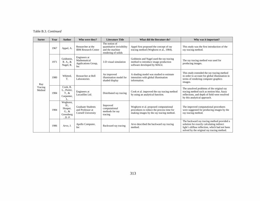
313

Table B.3. Continued

Sorter Year Author Who were they? Literature Title What did the literature do? Why was it important?

Ray

Tracing Method

1967 Appel, A. Researcher at the

IBM Research Center

The notion of

quantitative invisibility

and the machine rendering of solids

Appel first proposed the concept of ray

tracing method (Weghorst et al., 1984).

This study was the first introduction of the

ray tracing method.

1971

Goldstein,

R. A., &

Nagel, R.

Engineers at

Mathematical Applications Group,

Inc

3-D visual simulation

Goldstein and Nagel used the ray tracing

method to introduce image production

software developed by MAGI.

The ray tracing method was used for producing images.

1980 Whitted,

T.

Researcher at Bell

Laboratories

An improved

illumination model for shaded display

A shading model was studied to estimate

intensities with global illumination information.

This study extended the ray tracing method in order to account for global illumination in

terms of rendering computer graphics

images.

1984

Cook, R. L., Porter,

T., &

Carpenter, L.

Engineers at Lucasfilm Ltd.

Distributed ray tracing Cook et al. improved the ray tracing method by using an analytical function.

The unsolved problems of the original ray

tracing method such as motion blur, fuzzy reflections, and depth of field were resolved

by this analytical approach.

1984

Weghorst,

H.,

Hooper,

G., &

Greenberg, D. P.

Graduate Students

and Professor at Cornell University

Improved

computational

methods for ray

tracing

Weghorst et al. proposed computational

procedures to reduce the process time for making images by the ray tracing method.

The improved computational procedures

were suggested for producing images by the ray tracing method.

1986 Arvo, J. Apollo Computer,

Inc Backward ray tracing

Arvo described the backward ray tracing

method.

The backward ray tracing method provided a solution for exactly calculating indirect

light’s diffuse reflection, which had not been

solved by the original ray tracing method.