ORF 522: Lecture 1

Linear Programming: Chapter 1

Introduction

Robert J. Vanderbei

September 13, 2012

Slides last edited on September 13, 2012

Operations Research and Financial Engineering, Princeton University

http://www.princeton.edu/∼rvdb

Resource Allocation

maximize c1x1 + c2x2 + · · · + cnxnsubject to a11x1 + a12x2 + · · · + a1nxn ≤ b1

a21x1 + a22x2 + · · · + a2nxn ≤ b2...

am1x1 + am2x2 + · · · + amnxn ≤ bmx1, x2, ... , xn ≥ 0,

where

cj = profit per unit of product j produced

bi = units of raw material i on hand

aij = units of raw material i required to produce one unit of product j .

Blending Problems (Diet Problem)

minimize c1x1 + c2x2 + · · · + cnxnsubject to l1 ≤ a11x1 + a12x2 + · · · + a1nxn ≤ u1

l2 ≤ a21x1 + a22x2 + · · · + a2nxn ≤ u2...

lm ≤ am1x1 + am2x2 + · · · + amnxn ≤ umx1, x2, ... , xn ≥ 0 ,

where

cj = cost per unit of food jli = minimum daily allowance of nutrient i

ui = maximum daily allowance of nutrient iaij = units of nutrient i contained in one unit of food j .

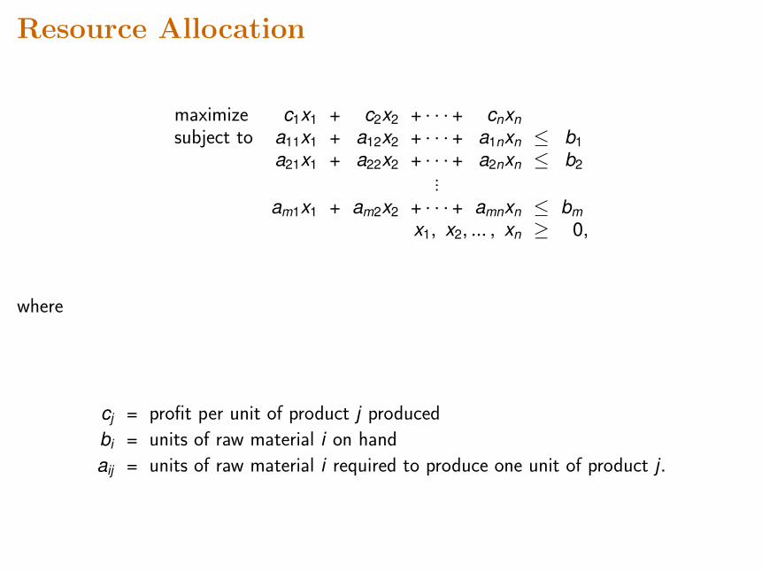
Fairness in Gradinga

MAT CHE ANT REL POL ECO GPA

John C+ B− B B+ 2.83Paul C+ B− B+ A− 3.00George C+ B− B+ A− 3.00Ringo B− B B+ A− 3.18Avg. 2.50 2.70 2.77 3.23 3.33 3.50

The Model

Paul got a B+ (3.3) in Politics.

We wish to assert that Paul’s actual grade plus a measure of the level of difficulty in Politicscourses equals Paul’s aptitude plus some small error:

Paul’s grade in Politics + Difficulty of Politics = Paul’s Aptitude + error term

Try to find numerical values for Aptitudes and Difficulties by minimizing the sum of the errorterms over all student/course grades.

a All characters appearing herein are fictitious. Any resemblance to real persons, living or dead, is purely coincidental.

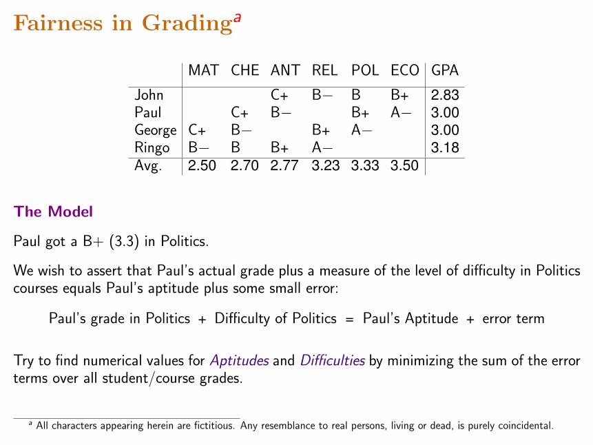
Minimizing The Sum Of The Errors

We don’t want negative errors to cancel with positive errors.

We could minimize the sum of the squares of the errors (least squares).

Or, we could minimize the sum of the absolute values of the errors (least absolute deviations).

I used the latter—it provides answers that are analogous to medians rather than simpleaverages (means).

Fixing a Point of Reference

The (course-enrollment weighted) sum of difficulties is constrained to be zero.

The Model

We assume that every grade, gi ,j for student i in course j , can be decomposed as a differencebetween

1. aptitude, ai , of student i , and

2. difficulty, dj , of course j ,

3. plus some small correction εi ,j .

That is,gi ,j = ai − dj + εi ,j .

The gi ,j ’s are data. We wish to find the ai ’s and the dj ’s that minimizes the sum of theabsolute values of the εi ,j ’s:

minimize∑

i ,j

|εi ,j |

subject to gi ,j = ai − dj + εi ,j for student-course pairs (i , j)∑j

dj = 0.

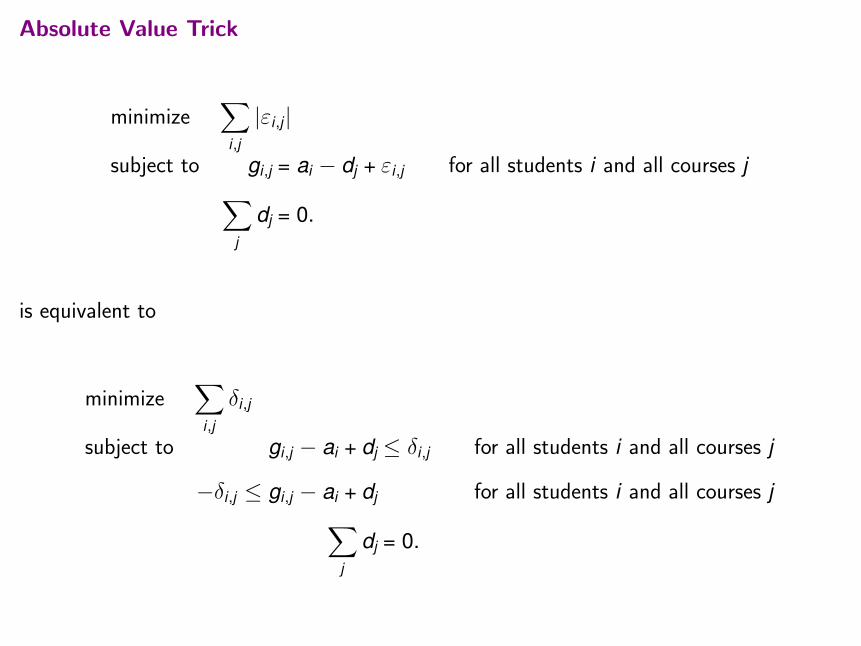
Absolute Value Trick

minimize∑

i ,j

|εi ,j |

subject to gi ,j = ai − dj + εi ,j for all students i and all courses j∑j

dj = 0.

is equivalent to

minimize∑

i ,j

δi ,j

subject to gi ,j − ai + dj ≤ δi ,j for all students i and all courses j

−δi ,j ≤ gi ,j − ai + dj for all students i and all courses j∑j

dj = 0.

The AMPL Model

set STUDS;set COURSES;

set GRADES within {STUDS, COURSES};

param grade {GRADES};

var aptitude {STUDS};

var difficulty {COURSES};

var dev {GRADES} >= 0;

minimize sum_dev: sum {(s,c) in GRADES} dev[s,c];

subject to def_pos_dev {(s,c) in GRADES}:

aptitude[s] - difficulty[c] - grade[s,c] <= dev[s,c];

subject to def_neg_dev {(s,c) in GRADES}:

-dev[s,c] <= aptitude[s] - difficulty[c] - grade[s,c];

subject to normalized_difficulty:

sum {c in COURSES} difficulty[c] = 0;

data;

set STUDS :=

John

Paul

George

Ringo

;

set COURSES :=MAT

CHE

ANT

REL

POL

ECO

;

param: GRADES: grade :=

John ANT 2.3

John REL 2.7

John POL 3

John ECO 3.3

Paul CHE 2.3

Paul ANT 2.7

Paul POL 3.3

Paul ECO 3.7

George MAT 2.3

George CHE 2.7

George REL 3.3

George POL 3.7

Ringo MAT 2.7

Ringo CHE 3

Ringo ANT 3.3

Ringo REL 3.7

;

solve;

display aptitude;

display difficulty;

AMPL Info

• The language is called AMPL, which stands for A Mathematical Programming Language.

• The “official” document describing the language is a book called “AMPL” by Fourer,Gay, and Kernighan. Amazon.com sells it for $78.01.

• There are also online tutorials:

– http://www.student.math.uwaterloo.ca/~co370/ampl/AMPLtutorial.pdf

– http://www.columbia.edu/~dano/courses/4600/lectures/6/AMPLTutorialV2.pdf

– https://webspace.utexas.edu/sdb382/www/teaching/ce4920/ampl_tutorial.pdf

– http://www2.isye.gatech.edu/~jswann/teaching/AMPLTutorial.pdf

– Google: “AMPL tutorial” for several more.

NEOS Info

NEOS is the Network Enabled Optimization Server supported by our federal government andlocated at Argonne National Lab.

To submit an AMPL model to NEOS...

• visit http://www.neos-server.org/neos/,

• click on the icon,

• scroll down to the Nonlinearly Constrained Optimization list,

• click on LOQO [AMPL input],

• scroll down to Model File:,

• click on Choose File,

• select a file from your computer that contains an AMPL model,

• scroll down to e-mail address:,

• type in your email address, and

• click Submit to NEOS.

Piece of cake!

Ringo Is Smarter Than You Thought

MAT CHE ANT REL POL ECO GPA Aptitude

John C+ B− B B+ 2.83 2.49Paul C+ B− B+ A− 3.00 2.84George C+ B− B+ A− 3.00 3.16Ringo B− B B+ A− 3.18 3.51Avg. 2.50 2.70 2.77 3.23 3.33 3.50Difficulty +0.84 +0.51 +0.19 −0.19 −0.51 −0.84

Paul’s grade in Politics + Difficulty of Politics = Paul’s Aptitude + error term

3.3 + (−0.51) = 2.84 + (−0.05)

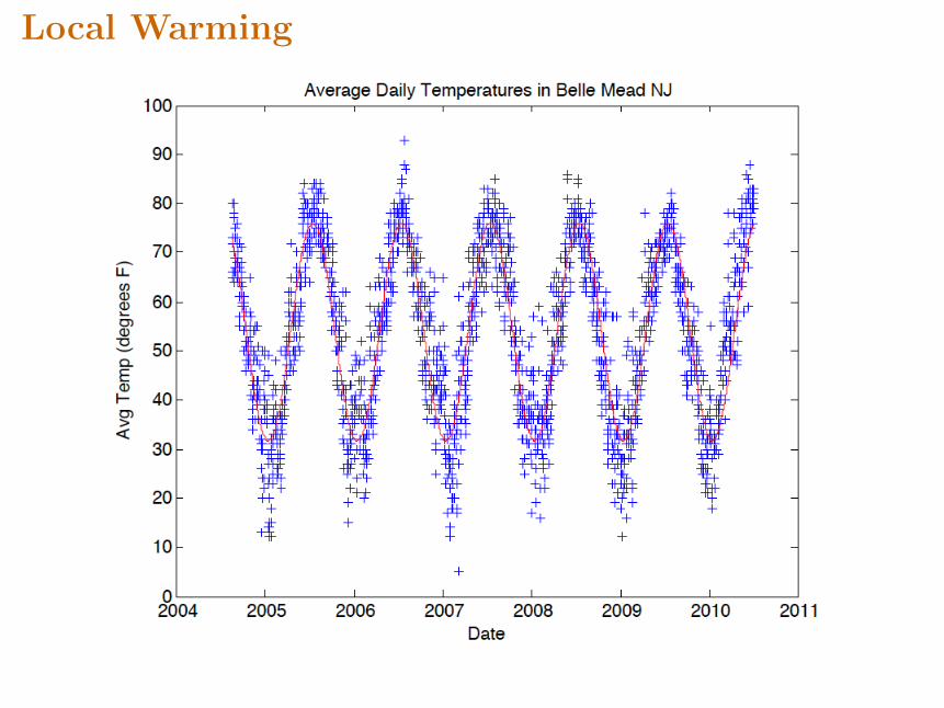
Local Warming

The Temperature Model

Assume daily average temperature has a sinusoidal annual variation superimposed on a lineartrend:

mina0,...,a3

∑d∈D

|a0 + a1d + a2 cos(2πd/365.25) + a3 sin(2πd/365.25)− Td |

Reformulate as a Linear Programming Model

Use the same absolute-value trick again:

minimize∑d∈D

δd

subject to −δd ≤ a0 + a1d + a2 cos(2πd/365.25) + a3 sin(2πd/365.25)− Td

a0 + a1d + a2 cos(2πd/365.25) + a3 sin(2πd/365.25)− Td ≤ δd

AMPL Modelset DATES ordered;

param hi {DATES};

param avg {DATES};

param lo {DATES};

param pi := 4*atan(1);

var a {j in 0..3};

var dev {DATES} >= 0, := 1;

minimize sumdev: sum {d in DATES} dev[d];

subject to def_pos_dev {d in DATES}:

a[0] + a[1]*ord(d,DATES) + a[2]*cos( 2*pi*ord(d,DATES)/365.25)

+ a[3]*sin( 2*pi*ord(d,DATES)/365.25) - avg[d]

<= dev[d];

subject to def_neg_dev {d in DATES}:

-dev[d] <=

a[0] + a[1]*ord(d,DATES) + a[2]*cos( 2*pi*ord(d,DATES)/365.25)

+ a[3]*sin( 2*pi*ord(d,DATES)/365.25) - avg[d];

data;

set DATES := include "dates.txt";

param: hi avg lo := include "WXDailyHistory.txt";

solve;

display a;

display a[1]*365.25;

It’s Getting Warmer in NJ

a[1]*365.25 = 0.0200462

A better model using 55 years of data from McGuire AFB here in NJ is described at

http://www.princeton.edu/~rvdb/ampl/nlmodels/LocalWarming/McGuireAFB/McGuire.html

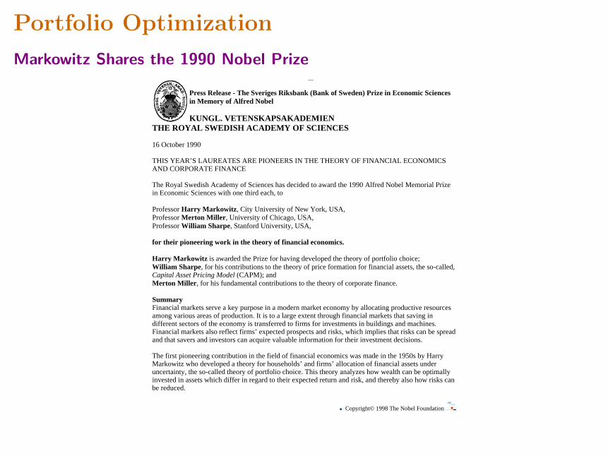
Portfolio Optimization

Markowitz Shares the 1990 Nobel Prize

Press Release - The Sveriges Riksbank (Bank of Sweden) Prize in Economic Sciencesin Memory of Alfred Nobel

KUNGL. VETENSKAPSAKADEMIEN THE ROYAL SWEDISH ACADEMY OF SCIENCES

16 October 1990

THIS YEAR’S LAUREATES ARE PIONEERS IN THE THEORY OF FINANCIAL ECONOMICSAND CORPORATE FINANCE

The Royal Swedish Academy of Sciences has decided to award the 1990 Alfred Nobel Memorial Prizein Economic Sciences with one third each, to

Professor Harry Markowitz, City University of New York, USA,Professor Merton Miller, University of Chicago, USA,Professor William Sharpe, Stanford University, USA,

for their pioneering work in the theory of financial economics.

Harry Markowitz is awarded the Prize for having developed the theory of portfolio choice; William Sharpe, for his contributions to the theory of price formation for financial assets, the so-called,Capital Asset Pricing Model (CAPM); andMerton Miller, for his fundamental contributions to the theory of corporate finance.

SummaryFinancial markets serve a key purpose in a modern market economy by allocating productive resourcesamong various areas of production. It is to a large extent through financial markets that saving indifferent sectors of the economy is transferred to firms for investments in buildings and machines.Financial markets also reflect firms’ expected prospects and risks, which implies that risks can be spreadand that savers and investors can acquire valuable information for their investment decisions.

The first pioneering contribution in the field of financial economics was made in the 1950s by HarryMarkowitz who developed a theory for households’ and firms’ allocation of financial assets underuncertainty, the so-called theory of portfolio choice. This theory analyzes how wealth can be optimallyinvested in assets which differ in regard to their expected return and risk, and thereby also how risks canbe reduced.

Copyright© 1998 The Nobel Foundation For help, info, credits or comments, see "About this project"

Last updated by Webmaster@www.nobel.se / February 25, 1997

Historical Data

Year US US S&P Wilshire NASDAQ Lehman EAFE Gold3-Month Gov. 500 5000 Composite Bros.

T-Bills Long Corp.Bonds Bonds

1973 1.075 0.942 0.852 0.815 0.698 1.023 0.851 1.6771974 1.084 1.020 0.735 0.716 0.662 1.002 0.768 1.7221975 1.061 1.056 1.371 1.385 1.318 1.123 1.354 0.7601976 1.052 1.175 1.236 1.266 1.280 1.156 1.025 0.9601977 1.055 1.002 0.926 0.974 1.093 1.030 1.181 1.2001978 1.077 0.982 1.064 1.093 1.146 1.012 1.326 1.2951979 1.109 0.978 1.184 1.256 1.307 1.023 1.048 2.2121980 1.127 0.947 1.323 1.337 1.367 1.031 1.226 1.2961981 1.156 1.003 0.949 0.963 0.990 1.073 0.977 0.6881982 1.117 1.465 1.215 1.187 1.213 1.311 0.981 1.0841983 1.092 0.985 1.224 1.235 1.217 1.080 1.237 0.8721984 1.103 1.159 1.061 1.030 0.903 1.150 1.074 0.8251985 1.080 1.366 1.316 1.326 1.333 1.213 1.562 1.0061986 1.063 1.309 1.186 1.161 1.086 1.156 1.694 1.2161987 1.061 0.925 1.052 1.023 0.959 1.023 1.246 1.2441988 1.071 1.086 1.165 1.179 1.165 1.076 1.283 0.8611989 1.087 1.212 1.316 1.292 1.204 1.142 1.105 0.9771990 1.080 1.054 0.968 0.938 0.830 1.083 0.766 0.9221991 1.057 1.193 1.304 1.342 1.594 1.161 1.121 0.9581992 1.036 1.079 1.076 1.090 1.174 1.076 0.878 0.9261993 1.031 1.217 1.100 1.113 1.162 1.110 1.326 1.1461994 1.045 0.889 1.012 0.999 0.968 0.965 1.078 0.990

Notation: Rj(t) = return on investment j in time period t .

Risk vs. Reward

Reward—estimated using historical means:

rewardj =1T

T∑t=1

Rj(t).

Risk—Markowitz defined risk as the variability of the returns as measured by the historicalvariances:

riskj =1T

T∑t=1

(Rj(t)− rewardj

)2 .

However, to get a linear programming problem (and for other reasonsa) we use the sum ofthe absolute values instead of the sum of the squares:

riskj =1T

T∑t=1

∣∣Rj(t)− rewardj∣∣ .

aSee http://www.princeton.edu/~rvdb/tex/lpport/lpport8.pdf

Hedging

Investment A: up 20%, down 10%, equally likely—a risky asset.

Investment B: up 20%, down 10%, equally likely—another risky asset.

Correlation: up years for A are down years for B and vice versa.

Portfolio—half in A, half in B: up 5% every year! No risk!

Portfolios

Fractions: xj = fraction of portfolio to invest in j .

Portfolio’s Historical Returns:R(t) =

∑j

xjRj(t)

Portfolio’s Reward:

reward(x) =1T

T∑t=1

R(t) =1T

T∑t=1

∑j

xjRj(t)

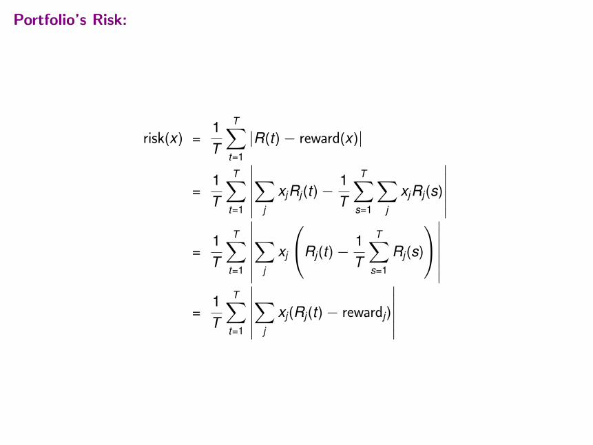
Portfolio’s Risk:

risk(x) =1T

T∑t=1

|R(t)− reward(x)|

=1T

T∑t=1

∣∣∣∣∣∣∑

j

xjRj(t)−1T

T∑s=1

∑j

xjRj(s)

∣∣∣∣∣∣=

1T

T∑t=1

∣∣∣∣∣∣∣∑

j

xj

Rj(t)−1T

T∑s=1

Rj(s)

∣∣∣∣∣∣∣

=1T

T∑t=1

∣∣∣∣∣∣∑

j

xj(Rj(t)− rewardj)

∣∣∣∣∣∣

A Markowitz-Type Model

Decision Variables: the fractions xj .

Objective: maximize return, minimize risk.

Fundamental Lesson: can’t simultaneously optimize two objectives.

Compromise: set an upper bound µ for risk and maximize reward subject to this boundconstraint:

• Parameter µ is called the risk aversion parameter.

• Large value for µ puts emphasis on reward maximization.

• Small value for µ puts emphasis on risk minimization.

Constraints:

1T

T∑t=1

∣∣∣∣∣∣∑

j

xj(Rj(t)− rewardj)

∣∣∣∣∣∣ ≤ µ

∑j

xj = 1

xj ≥ 0 for all j

Optimization Problem

maximize1T

T∑t=1

∑j

xjRj(t)

subject to1T

T∑t=1

∣∣∣∣∣∣∑

j

xj(Rj(t)− rewardj)

∣∣∣∣∣∣≤ µ∑j

xj = 1

xj ≥ 0 for all j

Because of absolute values not a linear programming problem.

Easy to convert (as we’ve already seen)...

A Linear Programming Formulation

maximize1T

T∑t=1

∑j

xjRj(t)

subject to −yt ≤∑

j

xj(Rj(t)− rewardj)≤ yt for all t

1T

T∑t=1

yt ≤ µ∑j

xj = 1

xj ≥ 0 for all j

Efficient Frontier

Varying risk bound µ produces the so-called efficient frontier.Portfolios on the efficient frontier are reasonable.Portfolios not on the efficient frontier can be strictly improved.

µ US Lehman NASDAQ Wilshire Gold EAFE Reward Risk3-Month Bros. Comp. 5000

T-Bills Corp.Bonds

0.1800 0.017 0.983 1.141 0.1800.1538 0.191 0.809 1.139 0.1540.1275 0.119 0.321 0.560 1.135 0.1280.1013 0.407 0.355 0.238 1.130 0.1010.0751 0.340 0.180 0.260 0.220 1.118 0.0750.0488 0.172 0.492 0.144 0.008 1.104 0.0490.0226 0.815 0.100 0.037 0.041 0.008 1.084 0.022

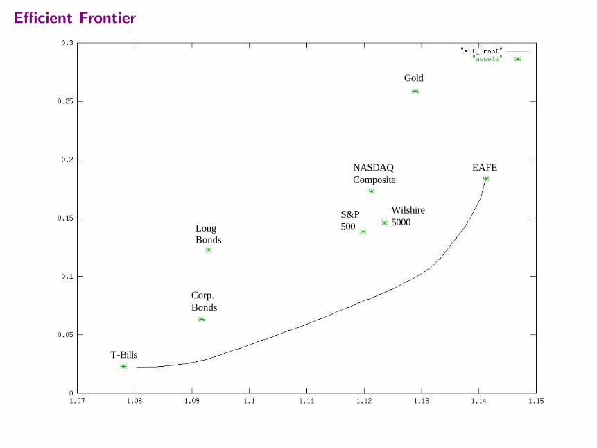
Efficient Frontier

T-Bills

Corp.Bonds

Long Bonds

S&P500

Wilshire5000

NASDAQComposite

Gold

EAFE