ANALYSIS Computable general equilibrium model analysis of ...
Upload
trinhxuyenCategory
view
224download
0
oranig06.doc revised March 2014
ORANI-G: A Generic Single-CountryComputable General Equilibrium Model
Mark Horridge
Centre of Policy Studies and Impact Project, Victoria University, Australia
Abstract:The ORANI applied general equilibrium (AGE) model of the Australian econ-omy has been widely used by academics and by economists in the government andprivate sectors. We describe a generic version of the model, ORANI-G, designed forexpository purposes and for adaptation to other countries.
Our description of the model's equations and database is closely integrated with anexplanation of how the model is solved using the GEMPACK system. The intention is toprovide a convenient starting-point for those wishing to use or construct a similar AGEmodel. Computer files are available, which contain a complete model specification anddatabase.
ORANI-G forms the basis of an annual modelling course, and has been adapted tobuild models of South Africa, Brazil, Ireland, Pakistan, Sri Lanka, Fiji, South Korea,Denmark, Vietnam, Thailand, Indonesia, Philippines and both Chinas.
Bibliographical Note: this document has its origin in the article"ORANI-F: A GeneralEquilibrium Model of the Australian Economy", by J.M. Horridge, B.R. Parmenter andK.R. Pearson (all of the Centre of Policy Studies), which appeared in the journal Eco-nomic and Financial Computing (vol.3,no.2,Summer 1993). This original version canbe found at http://www.copsmodels.com/archivep.htm#tpmh0139. SubsequentlyHorridge has progressively altered the article for teaching purposes, removingcontributions by the other authors.

ORANI-G is designed to be freely used and adapted for various countries and purposes. The same is trueof this document. You are welcome to use or alter all or parts of it to prepare documentation for yourown ORANI-G based model. However, we ask that you make some attribution or acknowledgement ifyou do use the document in this way. You can cite the document as follows:Horridge (2000), ORANI-G: A General Equilibrium Model of the Australian Economy, CoPS/IMPACT WorkingPaper Number OP-93, Centre of Policy Studies, Victoria University, downloadable from:
www.copsmodels.com/elecpapr/op-93.htm
Changes for the 2001 editionThis edition includes an expanded discussion of closures, changes reflecting advances in GEMPACKsoftware; and a reorganized TAB file. The changes to the TAB file are designed to make it morereadable, more modular, and easier to maintain. For example, instead of appearing in one huge list, mostvariables are declared immediately prior to the equations in which they appear (if desired, the softwarecan produce a comprehensive list of variables, such as appears in Appendix K). Also, an attempt hasbeen made to confine the effect of particular theoretical assumptions (such as the mechanism of a tax) tofewer (ideally, just one) equations. For example, update statements for tax flows and computations ofaggregate tax revenue are now independent of whether tax variables are expressed as powers or as advalorem rates. Again, the original version of ORANI used the assumptions of constant returns to scaleand marginal cost pricing to eliminate quantity variables from the industry zero pure profits (ZPP)condition. Those assumptions are not embedded in the ZPP equation for ORANIG01.
Changes for the 2003 editionThis edition includes new variables: p1var (short-run variable cost price index); x0gne, p0gne and w0gne(absorption aggregates); xgdpfac (GDP at factor cost, easily decomposed into components due to eachprimary factor). New real income-side GDP variable x0gdpinc equals x0gdpexp and can be decomposedinto primary factor, tech change and tax components. Some equations have been re-arranged to makethem more friendly to AnalyseGE. For the same reason, many substitutions were converted tobacksolves. Previously all parameters were positive except export demand elasticities and Frischparameters: now these also may be positive without error. The ID01 function is used instead of TINY insome places. TINY and ID01 appear in a few more places to combat rare zero-divide problems.
Changes for the 2005 editionThe TAB file (but not the text) contains some new macro variables to assist in explaining results. TheTAB file also contains an example of the “post-sim” calculations possible in Version 9 and later ofGEMPACK.
Latest ORANI-G-related material will be found at:
http://www.copsmodels.com/oranig.htm
This document was produced in MS Word97. It is designed to be printed on A4paper, and to be copied double-sided. In that case, even-numbered pages shouldappear on the left, and odd pages on the right, of each two-page spread. Forprinting, you might need to use some special fonts: the relevant files (with TTFextensions) should be included with the document file. Some other programswere used to produce diagrams: the Draw98 extension to Office97, MicroGrafxABC FlowCharter 2.0, and Deneba Canvas7SE.

Contents
1. Introduction 1
2. Model Structure and Interpretation of Results 2
2.1. A comparative-static interpretation of model results 2
3. The Percentage-Change Approach to Model Solution 3
3.1. Levels and linearised systems compared: a small example 5
3.2. The initial solution 6
4. The Equations of ORANI-G 7
4.1. The TABLO language 7
4.2. The model's data base 8
4.3. Dimensions of the model 10
4.4. The ORANI-G naming system 11
4.5. Core data coefficients and related variables 12
4.6. The equation system 17
4.7. Structure of production 17
4.8. Demands for primary factors 18
4.9. Sourcing of intermediate inputs 21
4.10. Top production nest 23
4.11. Industry costs and production taxes 24
4.12. From industry outputs to commodity ouputs 25
4.13. Export and local market versions of each good 26
4.14. Demands for investment goods 27
4.15. Household demands 28
4.16. Export demands 31
4.17. Other final demands 33
4.18. Demands for margins 34
4.19. Formulae for sales aggregates 34
4.20. Market-clearing equations 35
4.21. Purchasers' prices 35
4.22. Indirect taxes 37
4.23. GDP from the income and expenditure sides 40
4.24. The trade balance and other aggregates 43
4.25. Primary factor aggregates 43
4.26. Rates of return and investment 44
4.27. The labour market 46
4.28. Miscellaneous equations 46
4.29. Adding variables for explaining results 47
4.30. Sales decomposition 47
4.31. The Fan decomposition 48
4.32. The expenditure side GDP decomposition 49
4.33. Checking the data 51
4.34. Summarizing the data 51
4.35. Import shares and short-run supply elasticities 53
4.36. Storing Data for Other Computations 54
5. A Top-down Regional Extension 55
6. Closing the Model 56
7. Using GEMPACK to Solve the Model 59
8. Conclusion 61
References 63
Appendix A: Percentage-Change Equations of a CES Nest 64
Appendix B: ORANI-G on the World Wide Web 66

Appendix C: Hardware and Software Requirements for Using GEMPACK 66
Appendix D: Main differences between full-size ORANI and the version described here 67
Appendix E: Deriving Percentage-Change Forms 68
Appendix F: Algebra for the Linear Expenditure System 68
Appendix G: Making your own AGE model from ORANI-G 70
Appendix H: Additions and Changes for the 1998 edition 71
Appendix I: Formal Checks on Model Validity; Debugging Strategies 71
Appendix J: Short-Run Supply Elasticity 73
Appendix K: List of Variables 74
ORANI-G: A Generic Single-Country Computable General Equilibrium Model
1
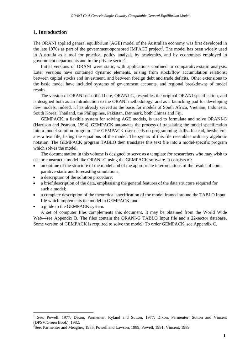
1. Introduction
The ORANI applied general equilibrium (AGE) model of the Australian economy was first developed inthe late 1970s as part of the government-sponsored IMPACT project1. The model has been widely usedin Australia as a tool for practical policy analysis by academics, and by economists employed ingovernment departments and in the private sector2.
Initial versions of ORANI were static, with applications confined to comparative-static analysis.Later versions have contained dynamic elements, arising from stock/flow accumulation relations:between capital stocks and investment, and between foreign debt and trade deficits. Other extensions tothe basic model have included systems of government accounts, and regional breakdowns of modelresults.
The version of ORANI described here, ORANI-G, resembles the original ORANI specification, andis designed both as an introduction to the ORANI methodology, and as a launching pad for developingnew models. Indeed, it has already served as the basis for models of South Africa, Vietnam, Indonesia,South Korea, Thailand, the Philippines, Pakistan, Denmark, both Chinas and Fiji.
GEMPACK, a flexible system for solving AGE models, is used to formulate and solve ORANI-G(Harrison and Pearson, 1994). GEMPACK automates the process of translating the model specificationinto a model solution program. The GEMPACK user needs no programming skills. Instead, he/she cre-ates a text file, listing the equations of the model. The syntax of this file resembles ordinary algebraicnotation. The GEMPACK program TABLO then translates this text file into a model-specific programwhich solves the model.
The documentation in this volume is designed to serve as a template for researchers who may wish touse or construct a model like ORANI-G using the GEMPACK software. It consists of: an outline of the structure of the model and of the appropriate interpretations of the results of com-
parative-static and forecasting simulations; a description of the solution procedure; a brief description of the data, emphasising the general features of the data structure required for
such a model; a complete description of the theoretical specification of the model framed around the TABLO Input
file which implements the model in GEMPACK; and a guide to the GEMPACK system.
A set of computer files complements this document. It may be obtained from the World WideWeb—see Appendix B. The files contain the ORANI-G TABLO Input file and a 22-sector database.Some version of GEMPACK is required to solve the model. To order GEMPACK, see Appendix C.
1 See: Powell, 1977; Dixon, Parmenter, Ryland and Sutton, 1977; Dixon, Parmenter, Sutton and Vincent(DPSV/Green Book), 1982.2See: Parmenter and Meagher, 1985; Powell and Lawson, 1989, Powell, 1991; Vincent, 1989.
Mark Horridge
2
2. Model Structure and Interpretation of Results
ORANI-G has a theoretical structure which is typical of a static AGE model. It consists of equations de-scribing, for some time period: producers' demands for produced inputs and primary factors; producers' supplies of commodities; demands for inputs to capital formation; household demands; export demands; government demands; the relationship of basic values to production costs and to purchasers' prices; market-clearing conditions for commodities and primary factors; and numerous macroeconomic variables and price indices.Demand and supply equations for private-sector agents are derived from the solutions to the optimisationproblems (cost minimisation, utility maximisation, etc.) which are assumed to underlie the behaviour ofthe agents in conventional neoclassical microeconomics. The agents are assumed to be price-takers, withproducers operating in competitive markets which prevent the earning of pure profits.
2.1. A comparative-static interpretation of model results
Like the majority of AGE models, ORANI-G is designed for comparative-static simulations. Itsequations and variables, which are described in detail in Section 4, all refer implicitly to the economy atsome future time period.
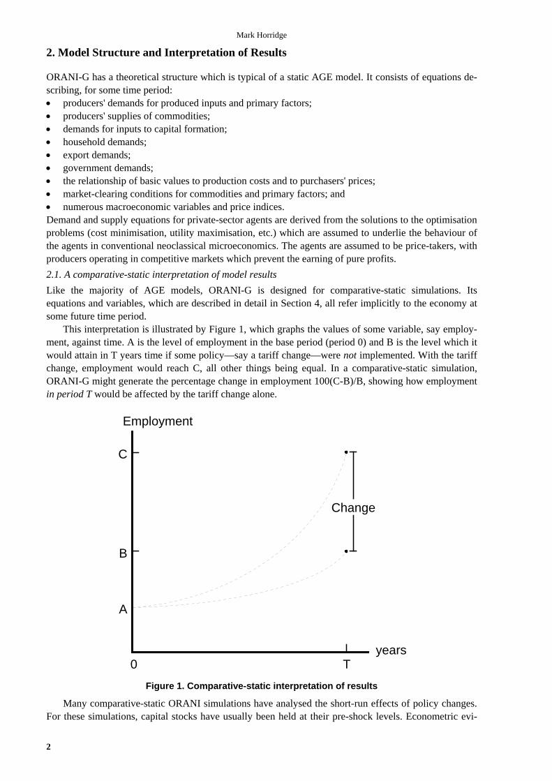
This interpretation is illustrated by Figure 1, which graphs the values of some variable, say employ-ment, against time. A is the level of employment in the base period (period 0) and B is the level which itwould attain in T years time if some policy—say a tariff change—were not implemented. With the tariffchange, employment would reach C, all other things being equal. In a comparative-static simulation,ORANI-G might generate the percentage change in employment 100(C-B)/B, showing how employmentin period T would be affected by the tariff change alone.
Employment
0 T
Change
A
years
B
C
Figure 1. Comparative-static interpretation of results
Many comparative-static ORANI simulations have analysed the short-run effects of policy changes.For these simulations, capital stocks have usually been held at their pre-shock levels. Econometric evi-

ORANI-G: A Generic Single-Country Computable General Equilibrium Model
3
dence suggests that a short-run equilibrium will be reached in about two years, i.e., T=2 (Cooper,McLaren and Powell, 1985). Other simulations have adopted the long-run assumption that capital stockswill have adjusted to restore (exogenous) rates of return—this might take 10 or 20 years, i.e., T=10 or20. In either case, only the choice of closure and the interpretation of results bear on the timing ofchanges: the model itself is atemporal. Consequently it tells us nothing of adjustment paths, shown asdotted lines in Figure 1.
There are also various dynamic versions of ORANI, to which this document refers only in passing.Results from the dynamic versions are also reported in percentage change form. Here, however, thechanges compare two different instants in time. For example, in terms of Figure 1, results from a baseforecast might refer to the change from A to B. Another set of results, incorporating the changed tariff,would refer to the change from A to C.
The dynamic versions of ORANI3 generally incorporate investment-capital accumulation relationswhich explicitly mention the length of the period T. A more important practical difference between dy-namic and comparative-static applications is that dynamic models require far more information aboutchanges in exogenous variables. Comparative-static simulation of the change from B to C requires, inaddition to the initial database, only the value of the exogenous tariff change. For a dynamic simulationwe must specify changes in all exogenous variables. Thus we would need to forecast changes in foreignprices, in all sorts of tax rates, in technology and in tastes.
For these dynamic models, T is usually set to 1. A sequence of annual solutions are linked together,so that a complete forecast consists of a series of year-on-year changes for all of its many thousands ofvariables. By computing annual solutions, we are able to be fairly explicit about adjustment processes.The disadvantage, as mentioned above, is that the modeller is forced to postulate the future time-path ofvery many exogenous variables.
3. The Percentage-Change Approach to Model Solution
Many of the ORANI-G equations are non-linear—demands depend on price ratios, for example. How-ever, following Johansen (1960), the model is solved by representing it as a series of linear equationsrelating percentage changes in model variables. This section explains how the linearised form can beused to generate exact solutions of the underlying, non-linear, equations, as well as to compute linearapproximations to those solutions4.
A typical AGE model can be represented in the levels as:
F(Y,X) = 0, (1)
where Y is a vector of endogenous variables, X is a vector of exogenous variables and F is a system ofnon-linear functions. The problem is to compute Y, given X. Normally we cannot write Y as an explicitfunction of X.
Several techniques have been devised for computing Y. The linearised approach starts by assumingthat we already possess some solution to the system, {Y0,X0}, i.e.,
F(Y0,X0) = 0. (2)
Normally the initial solution {Y0,X0} is drawn from historical data—we assume that our equation systemwas true for some point in the past. With conventional assumptions about the form of the F function itwill be true that for small changes dY and dX:
FY(Y,X)dY + FX(Y,X)dX = 0, (3)
where FY and FX are matrices of the derivatives of F with respect to Y and X, evaluated at {Y0,X0}. Forreasons explained below, we find it more convenient to express dY and dX as small percentage changesy and x. Thus y and x, some typical elements of y and x, are given by:
y = 100dY/Y and x = 100dX/X. (4)
3 ORANIG-RD, a dynamic version of ORANI-G, may be downloaded from the ORANI-G web page.4 For a detailed treatment of the linearised approach to AGE modelling, see the Black Book. Chapter 3 contains in-formation about Euler's method and multistep computations.

Mark Horridge
4
Correspondingly, we define:
GY(Y,X) = FY(Y,X)Y^ and GX(Y,X) = FX(Y,X)X^ , (5)
where Y^ and X^ are diagonal matrices. Hence the linearised system becomes:
GY(Y,X)y + GX(Y,X)x = 0. (6)
Such systems are easy for computers to solve, using standard techniques of linear algebra. But they areaccurate only for small changes in Y and X. Otherwise, linearisation error may occur. The error is illus-trated by Figure 2, which shows how some endogenous variable Y changes as an exogenous variable Xmoves from X0 to XF. The true, non-linear relation between X and Y is shown as a curve. The linear, orfirst-order, approximation:
y = - GY(Y,X)-1GX(Y,X)x (7)
leads to the Johansen estimate YJ—an approximation to the true answer, Yexact.
Y1 step
Exact
XX0 X
Y0
Yexact
F
YJ
dX
dY
Figure 2. Linearisation error
Figure 2 suggests that, the larger is x, the greater is the proportional error in y. This observation leadsto the idea of breaking large changes in X into a number of steps, as shown in Figure 3. For each sub-change in X, we use the linear approximation to derive the consequent sub-change in Y. Then, using thenew values of X and Y, we recompute the coefficient matrices GY and GX. The process is repeated foreach step. If we use 3 steps (see Figure 3), the final value of Y, Y3, is closer to Yexact than was the Johan-sen estimate YJ. We can show, in fact, that given sensible restrictions on the derivatives of F(Y,X), wecan obtain a solution as accurate as we like by dividing the process into sufficiently many steps.
The technique illustrated in Figure 3, known as the Euler method, is the simplest of several relatedtechniques of numerical integration—the process of using differential equations (change formulae) tomove from one solution to another. GEMPACK offers the choice of several such techniques. Each re-quires the user to supply an initial solution {Y0,X0}, formulae for the derivative matrices GY and GX,and the total percentage change in the exogenous variables, x. The levels functional form, F(Y,X), neednot be specified, although it underlies GY and GX.
The accuracy of multistep solution techniques can be improved by extrapolation. Suppose the sameexperiment were repeated using 4-step, 8-step and 16-step Euler computations, yielding the followingestimates for the total percentage change in some endogenous variable Y:
y(4-step) = 4.5%,y(8-step) = 4.3% (0.2% less), andy(16-step) = 4.2% (0.1% less).
Extrapolation suggests that the 32-step solution would be:y(32-step) = 4.15% (0.05% less),
and that the exact solution would be:y(-step) = 4.1%.

ORANI-G: A Generic Single-Country Computable General Equilibrium Model
5
Y1 step
3 step
Exact
XX0 X1 X2 X3
Y0
Y1
Y3
Yexact
Y2
XF
YJ
Figure 3. Multistep process to reduce linearisation error
The extrapolated result requires 28 (= 4+8+16) steps to compute but would normally be more accuratethan that given by a single 28-step computation. Alternatively, extrapolation enables us to obtain givenaccuracy with fewer steps. As we noted above, each step of a multi-step solution requires: computationfrom data of the percentage-change derivative matrices GY and GX; solution of the linear system (6); anduse of that solution to update the data (X,Y).
In practice, for typical AGE models, it is unnecessary, during a multistep computation, to recordvalues for every element in X and Y. Instead, we can define a set of data coefficients V, which are func-tions of X and Y, i.e., V = H(X,Y). Most elements of V are simple cost or expenditure flows such asappear in input-output tables. GY and GX turn out to be simple functions of V; often indeed identical toelements of V. After each small change, V is updated using the formula v = HY(X,Y)y + HX(X,Y)x. Theadvantages of storing V, rather than X and Y, are twofold: the expressions for GY and GX in terms of V tend to be simple, often far simpler than the original F
functions; and there are fewer elements in V than in X and Y (e.g., instead of storing prices and quantities sepa-
rately, we store merely their products, the values of commodity or factor flows).
3.1. Levels and linearised systems compared: a small example
To illustrate the convenience of the linear approach5, we consider a very small equation system: the CESinput demand equations for a producer who makes output Z from N inputs Xk, k=1-N, with prices Pk. Inthe levels the equations are (see Appendix A):
Xk = Z /(k [ Pk
Pave]/(
, k=1,N (8)
where Pave = (i=1
N
/(i P
/(i )
. (9)
The k and are behavioural parameters. To solve the model in the levels, the values of the k are nor-mally found from historical flows data, Vk=PkXk, presumed consistent with the equation system andwith some externally given value for . This process is called calibration. To fix the Xk, it is usual to as-sign arbitrary values to the Pk, say 1. This merely sets convenient units for the Xk (base-period-dollars-worth). is normally given by econometric estimates of the elasticity of substitution, (=1/(+1)). Withthe Pk, Xk, Z and known, the k can be deduced.
In the solution phase of the levels model, k and are fixed at their calibrated values. The solutionalgorithm attempts to find Pk, Xk and Z consistent with the levels equations and with other exogenous
5 For a comparison of the levels and linearised approaches to solving AGE models see Hertel, Horridge & Pearson(1992).

Mark Horridge
6
restrictions. Typically this will involve repeated evaluation of both (8) and (9)—corresponding toF(Y,X)—and of derivatives which come from these equations—corresponding to FY and FX.
The percentage-change approach is far simpler. Corresponding to (8) and (9), the linearised equa-tions are (see Appendices A and E):
xk = z - (pk - pave), k=1,N (10)
and pave = i=1
N
Sipi, where the Si are cost shares, eg, Si= Vi / k=1
N
Vk (11)
Since percentage changes have no units, the calibration phase—which amounts to an arbitrary choice ofunits—is not required. For the same reason the k parameters do not appear. However, the flows data Vkagain form the starting point. After each change they are updated by:
Vk,new =Vk,old + Vk,old(xk + pk)/100 (12)
GEMPACK is designed to make the linear solution process as easy as possible. The user specifiesthe linear equations (10) and (11) and the update formulae (12) in the TABLO language—which re-sembles algebraic notation. Then GEMPACK repeatedly: evaluates GY and GX at given values of V; solves the linear system to find y, taking advantage of the sparsity of GY and GX; and updates the data coefficients V.The housekeeping details of multistep and extrapolated solutions are hidden from the user.
Apart from its simplicity, the linearised approach has three further advantages. It allows free choice of which variables are to be exogenous or endogenous. Many levels algorithms
do not allow this flexibility. To reduce AGE models to manageable size, it is often necessary to use model equations to substitute
out matrix variables of large dimensions. In a linear system, we can always make any variable thesubject of any equation in which it appears. Hence, substitution is a simple mechanical process. Infact, because GEMPACK performs this routine algebra for the user, the model can be specified interms of its original behavioural equations, rather than in a reduced form. This reduces the potentialfor error and makes model equations easier to check.
Perhaps most importantly, the linearized equations help us understand simulation results. We caneasily see the contribution of (the change in) each RHS variable to the LHS of each equation. Forexample, in the CES price index equation:
pave = i=1
N
Sipi
we can identify the contribution of each individual price pi to the index pave. The GEMPACKprogram AnalyseGE automates this task.
3.2. The initial solution
Our discussion of the solution procedure has so far assumed that we possess an initial solution of themodel—{Y0,X0} or the equivalent V0—and that results show percentage deviations from this initialstate.
In practice, the ORANI database does not, like B in Figure 1, show the expected state of the econ-omy at a future date. Instead the most recently available historical data, A, are used. At best, these referto the present-day economy. Note that, for the atemporal static model, A provides a solution for period T.In the static model, setting all exogenous variables at their base-period levels would leave all the en-dogenous variables at their base-period levels. Nevertheless, A may not be an empirically plausiblecontrol state for the economy at period T and the question therefore arises: are estimates of the B-to-Cpercentage changes much affected by starting from A rather than B? For example, would the percentageeffects of a tariff cut inflicted in 1994 differ much from those caused by a 2005 cut? Probably not. First,balanced growth, i.e., a proportional enlargement of the model database, just scales equation coefficientsequally; it does not affect ORANI results. Second, compositional changes, which do alter percentage-
ORANI-G: A Generic Single-Country Computable General Equilibrium Model
7
change effects, happen quite slowly. So for short- and medium-run simulations A is a reasonable proxyfor B, (Dixon, Parmenter and Rimmer, 1986).6
4. The Equations of ORANI-G
In this section we provide a formal description of the linear form of the model. Our description is organ-ised around the TABLO file which implements the model in GEMPACK. We present the complete textof the TABLO Input file divided into a sequence of excerpts and supplemented by tables, figures and ex-planatory text.
The TABLO language in which the file is written is essentially conventional algebra, with names forvariables and coefficients chosen to be suggestive of their economic interpretations. Some practice isrequired for readers to become familiar with the TABLO notation but it is no more complex than alterna-tive means of setting out the model—the notation employed in DPSV (1982), for example. Acquiring thefamiliarity allows ready access to the GEMPACK programs used to conduct simulations with the modeland to convert the results to human-readable form. Both the input and the output of these programs em-ploy the TABLO notation. Moreover, familiarity with the TABLO format is essential for users who maywish to make modifications to the model's structure.
Another compelling reason for using the TABLO Input file to document the model is that it ensuresthat our description is complete and accurate: complete because the only other data needed by theGEMPACK solution process is numerical (the model's database and the exogenous inputs to particularsimulations); and accurate because GEMPACK is nothing more than an equation solving system, incor-porating no economic assumptions of its own.
We continue this section with a short introduction to the TABLO language—other details may bepicked up later, as they are encountered. Then we describe the input-output database which underlies themodel. This structures our subsequent presentation.
4.1. The TABLO language
The TABLO model description defines the percentage-change equations of the model. For example, theCES demand equations, (10) and (11), would appear as:
Equation E_x # input demands # (all, f, FAC) x(f) = z ‐ SIGMA*[p(f) ‐ p_f]; Equation E_p_f # input cost index # V_F*p_f = sum{f,FAC, V(f)*p(f)};
The first word, 'Equation', is a keyword which defines the statement type. Then follows the identifier forthe equation, which must be unique. The descriptive text between '#' symbols is optional—it appears incertain report files. The expression '(all, f, FAC)' signifies that the equation is a matrix equation, contain-ing one scalar equation for each element of the set FAC.7
Within the equation, the convention is followed of using lower-case letters for the percentage-changevariables (x, z, p and p_f), and upper case for the coefficients (SIGMA, V and V_F). Since GEMPACKignores case, this practice assists only the human reader. An implication is that we cannot use the samesequence of characters, distinguished only by case, to define a variable and a coefficient. The '(f)' suffixindicates that variables and coefficients are vectors, with elements corresponding to the set FAC. A semi-colon signals the end of the TABLO statement.
6 We claim here that, for example, the estimate that a reduction in the textile tariff would reduce textileemployment 5 years hence by, say, 7%, is not too sensitive to the fact that our simulation started from today'sdatabase rather than a database representing the economy in 5 years time. Nevertheless, the social implications of a7% employment loss depend closely on whether textile employment is projected to grow in the absence of anytariff cut. To examine this question we need a forecasting model. If the base forecast scenario had textile employ-ment grow annually by 1.5%, the 7% reduction could be absorbed without actually firing any textile workers.7 For equation E_x we could have written: (all, j, FAC) x(j) = z - SIGMA*[p(j) - p_f], without affecting simulationresults. Our convention that the index, (f), be the same as the initial letter of the set it ranges over, aids comprehen-sion but is not enforced by GEMPACK. By contrast, GAMS (a competing software package) enforces consistentusage of set indices by rigidly connecting indices with the corresponding sets.
Mark Horridge
8
To facilitate portability between computing environments, the TABLO character set is quite re-stricted—only alphanumerics and a few punctuation marks may be used. The use of Greek letters andsubscripts is precluded, and the asterisk, '*', must replace the multiplication symbol ''.
Sets, coefficients and variables must be explicitly declared, via statements such as:
Set FAC # inputs # (capital, labour, energy);Coefficient (all,f,FAC) V(f) # cost of inputs #; V_F # total cost #; SIGMA # substitution elasticity #;Variable (all,f,FAC) p(f) # price of inputs #; (all,f,FAC) x(f) # demand for inputs #; z # output #; p_f # input cost index #;
As the last two statements in the 'Coefficient' block and the last three in the 'Variable' block illustrate,initial keywords (such as 'Coefficient' and 'Variable') may be omitted if the previous statement was of thesame type.
Coefficients must be assigned values, either by reading from file:
Read V from file FLOWDATA; Read SIGMA from file PARAMS;
or in terms of other coefficients, using formulae:
Formula V_F = sum{f, FAC, V(f)}; ! used in cost index equation !
The right hand side of the last statement employs the TABLO summation notation, equivalent to the notation used in standard algebra. It defines the sum over an index f running over the set FAC of the in-put-cost coefficients, V(f). The statement also contains a comment, i.e., the text between exclamationmarks (!). TABLO ignores comments.
Some of the coefficients will be updated during multistep computations. This requires the inclusionof statements such as:
Update (all,f,FAC) V(f) = x(f)*p(f);
which is the default update statement, causing V(f) to be increased after each step by [x(f) + p(f)]%,where x(f) and p(f) are the percentage changes computed at the previous step.
The sample statements listed above introduce most of the types of statement required for the model.But since all sets, variables and coefficients must be defined before they are used, and since coefficientsmust be assigned values before appearing in equations, it is necessary for the order of the TABLO state-ments to be almost the reverse of the order in which they appear above. The ORANI-G TABLO Inputfile is ordered as follows: definition of sets; declarations of variables; declarations of often-used coefficients which are read from files, with associated Read and Update
statements; declarations of other often-used coefficients which are computed from the data, using associated
Formulae; and groups of topically-related equations, with some of the groups including statements defining coeffi-
cients which are used only within that group.
4.2. The model's data base
Figure 4 is a schematic representation of the model's input-output database. It reveals the basic structureof the model. The column headings in the main part of the figure (an absorption matrix) identify thefollowing demanders:(1) domestic producers divided into I industries;(2) investors divided into I industries;(3) a single representative household;(4) an aggregate foreign purchaser of exports;

ORANI-G: A Generic Single-Country Computable General Equilibrium Model
9
(5) government demands; and(6) changes in inventories.
Absorption Matrix
1 2 3 4 5 6
Producers Investors Household Export GovernmentChange inInventories
Size I I 1 1 1 1
Basic
Flows
CS
V1BAS V2BAS V3BAS V4BAS V5BAS V6BAS
Margins
CSM
V1MAR V2MAR V3MAR V4MAR V5MAR n/a
Taxes
CS
V1TAX V2TAX V3TAX V4TAX V5TAX n/a
Labour
O
V1LAB
C = Number of Commodities
I = Number of Industries
Capital
1
V1CAP
S = 2: Domestic,Imported,
O = Number of Occupation Types
Land
1
V1LND
M = Number of Commodities used as Margins
Production
Tax
1
V1PTX
Other
Costs
1
V1OCT
Joint Produc-
tion MatrixImport Duty
Size I Size 1C
MAKE
C
V0TAR
Figure 4. The ORANI-G Flows Database
The entries in each column show the structure of the purchases made by the agents identified in thecolumn heading. Each of the C commodity types identified in the model can be obtained locally or im-ported from overseas. The source-specific commodities are used by industries as inputs to current pro-duction and capital formation, are consumed by households and governments, are exported, or are addedto or subtracted from inventories. Only domestically produced goods appear in the export column. M ofthe domestically produced goods are used as margins services (wholesale and retail trade, and transport)which are required to transfer commodities from their sources to their users. Commodity taxes arepayable on the purchases. As well as intermediate inputs, current production requires inputs of threecategories of primary factors: labour (divided into O occupations), fixed capital, and agricultural land.Production taxes include output taxes or subsidies that are not user-specific. The 'other costs' categorycovers various miscellaneous taxes on firms, such as municipal taxes or charges.

Mark Horridge
10
Each cell in the illustrative absorption matrix in Figure 4 contains the name of the correspondingdata matrix. For example, V2MAR is a 4-dimensional array showing the cost of M margins services onthe flows of C goods, both domestically produced and imported (S), to I investors.
In principle, each industry is capable of producing any of the C commodity types. The MAKE ma-trix at the bottom of Figure 4 shows the value of output of each commodity by each industry. Finally,tariffs on imports are assumed to be levied at rates which vary by commodity but not by user. The reve-nue obtained is represented by the tariff vector V0TAR.
4.3. Dimensions of the model
Excerpt 1 of the TABLO Input file begins by defining logical names for input and output files. Initialdata are stored in the BASEDATA input file. The SUMMARY output file is used to store summary anddiagnostic information. Note that BASEDATA and SUMMARY are logical names. The actual locationsof these files (disk, folder, filename) are chosen by the model user.
The rest of Excerpt 1 defines sets: lists of descriptors for the components of vector variables. Setnames appear in upper-case characters. For example, the first Set statement is to be read as defining a setnamed 'COM' which contains commodity descriptors. The elements of COM (a list of commoditynames) are read from the input file (this allows the model to use databases with different numbers ofsectors). By contrast the two elements of the set SRC—dom and imp—are listed explicitly.
! Excerpt 1 of TABLO input file: !! Files and sets !
File BASEDATA # Input data file #; (new) SUMMARY # Output for summary and checking data #;
Set !Index! COM # Commodities# read elements from file BASEDATA header "COM"; ! c ! SRC # Source of commodities # (dom,imp); ! s ! IND # Industries # read elements from file BASEDATA header "IND"; ! i ! OCC # Occupations # read elements from file BASEDATA header "OCC"; ! o ! MAR # Margin commodities # read elements from file BASEDATA header "MAR";! m !Subset MAR is subset of COM;Set NONMAR # Non‐margin commodities # = COM ‐ MAR; ! n !
The commodity, industry, and occupational classifications of the Australian version of ORANI-Gdescribed here are aggregates of the classifications used in the original version of ORANI, which hadover 100 industries and commodities, and 8 labour occupations.
The industry classification differs slightly from the commodity classification. Both are listed inTable 1. In this aggregated version of the model, multiproduction is confined to the first two industries,which produce the first three commodities. Each of the remaining industries produces a unique com-modity. Labour is disaggregated into skill-based occupational categories described by the set OCC.
The central column of Table 1 lists the elements of the set COM which are read from file.GEMPACK uses the element names to label the rows and columns of results and data tables. The ele-ment names cannot be more than 12 letters long, nor contain spaces. The IND elements are the same aselements 2-23 of COM.
Elements of the set MAR are margins commodities, i.e., they are required to facilitate the flows ofother commodities from producers (or importers) to users. Hence, the costs of margins services, togetherwith indirect taxes, account for differences between basic prices (received by producers or importers)and purchasers' prices (paid by users).
TABLO does not prevent elements of two sets from sharing the same name; nor, in such a case, doesit automatically infer any connection between the corresponding elements. The Subset statement whichfollows the definition of the set MAR is required for TABLO to realize that the two elements of MAR,Trade and Transport, are the same as the 18th and 19th elements of the set COM.
The statement for NONMAR defines that set as a complement. That is, NONMAR consists of allthose elements of COM which are not in MAR. In this case TABLO is able to deduce that NONMARmust be a subset of COM.

ORANI-G: A Generic Single-Country Computable General Equilibrium Model
11
Table 1 Commodity and Industry Classification
Commodity Description Elements of Set COM Industry Description
123
CerealsBroadacre ruralIntensive rural
CerealsAgBroadacreAgIntensive
12
Broadacre ruralIntensive rural
4 Mining, export MiningExport 3 Mining, export
5 Mining, other MiningOther 4 Mining, other
6 Food & fibre, export FoodFibre 5 Food & fibre, export
7 Food, other FoodOther 6 Food, other
8 Textiles, clothing & footwear TCF 7 Textiles, clothing & footwear
9 Wood related products WoodProds 8 Wood related products
10 Chemicals & oil products ChemProds 9 Chemicals & oil products
11 Non-metallic mineral products NonMetal 10 Non-metallic mineral products
12 Metal products MetalProds 11 Metal products
13 Transport equipment TrnspEquip 12 Transport equipment
14 Other machinery OthMachnry 13 Other machinery
15 Other manufacturing OthManufact 14 Other manufacturing
16 Utilities Utilities 15 Utilities
17 Construction Construction 16 Construction
18 Retail & wholesale trade Trade (margin) 17 Retail & wholesale trade
19 Transport Transport (margin) 18 Transport
20 Banking & finance Finance 19 Banking & finance
21 Ownership of dwellings Dwellings 20 Ownership of dwellings
22 Public services PublicServcs 21 Public services
23 Private services PrivatServcs 22 Private services
4.4. The ORANI-G naming system
The TABLO Input file defines a multitude of variables and coefficients that are used in the model'sequations. It can be difficult to remember the names of all these variables and coefficients8. Fortunately,their names follow a pattern. Although GEMPACK does not require that names conform to any pattern,we find that systematic naming reduces the burden on (human) memory. As far as possible, names forvariables and coefficients conform to a system in which each name consists of 2 or more parts, as fol-lows:
first, a letter or letters indicating the type of variable, for example,a technical changedel ordinary (rather than percentage) changef shift variableH indexing parameterp price, local currencypf price, foreign currencyS input shareSIGMA elasticity of substitutiont taxV levels value, local currencyw percentage-change value, local currencyx input quantity;
second, one of the digits 0 to 6 indicating user, that is,
8 GEMPACK's TABmate editor offers some comfort to the forgetful. With the TABLO Input file open inTABmate, you may click on any variable or coefficient name, then click the Gloss button. A list will appear,starting with a description of that variable and then showing all statements in the TABLO Input file where it isused.

Mark Horridge
12
1 current production2 investment3 consumption4 export5 government6 inventories0 all users, or user distinction irrelevant;
third (optional), three or more letters giving further information, for example,bas (often omitted) basic—not including margins or taxescap capitalcif imports at border pricesimp imports (duty paid)lab labourlnd landlux linear expenditure system (supernumerary part)mar marginsoct other cost ticketsprim all primary factors (land, labour or capital)pur at purchasers' pricessub linear expenditure system (subsistence part)tar tariffstax indirect taxestot total or average over all inputs for some user;
fourth (optional), an underscore character, indicating that this variable is an aggregate or average,with subsequent letters showing over which sets the underlying variable has been summed or aver-aged, for example,
_c over COM (commodities),_s over SRC (dom + imp),_i over IND (industries),_io over IND and OCC (skills).
Although GEMPACK does not distinguish between upper and lower case, we use:lower case for variable names and set indices;upper case for set and coefficient names; andinitial letter upper case for TABLO keywords.
4.5. Core data coefficients and related variables
The next excerpts of the TABLO file contains statements indicating data to be read from file. The dataitems defined in these statements appear as coefficients in the model's equations. The statements definecoefficient names (which all appear in upper-case characters), the locations from which the data are to beread, variable names (in lower-case), and formulae for the data updates which are necessary in com-puting multi-step solutions to the model (see Section 3).
4.5.1. Basic flows
The excerpts group the data according to the rows of Figure 4. Thus, Excerpt 2 begins by defining coef-ficients representing the basic commodity flows corresponding to row 1 (direct flows) of the figure, i.e.,the flow matrices V1BAS, V2BAS, and so on. Preceding the coefficient names are their dimensions,indicated using the "all" qualifier and the sets defined in Excerpt 1. For example, the first 'Coefficient'statement defines a data item V1BAS(c,s,i) which is the basic value (indicated by 'BAS') of a flow ofintermediate inputs (indicated by '1') of commodity c from source s to user industry i. The first 'Read'statement indicates that this data item is stored on file BASEDATA with header '1BAS'. (A GEMPACKdata file consists of a number of data items such as arrays of real numbers. Each data item is identifiedby a unique key or 'header').
Each of these flows is the product of a price and a quantity. The excerpt goes on to define thesevariables. Unless otherwise stated, all variables are percentage changes—to indicate this, their names

ORANI-G: A Generic Single-Country Computable General Equilibrium Model
13
appear in lower-case letters. Preceding the names of the variables are their dimensions, indicated usingthe sets defined in Excerpt 1. For example, the first variable statement defines a matrix variable x1 (in-dexed by commodity, source, and using industry) the elements of which are percentage changes in thedirect demands by producers for source-specific intermediate inputs. This is the quantity variable corre-sponding to V1BAS.
! Excerpt 2 of TABLO input file: !! Data coefficients and variables relating to basic commodity flows !
Coefficient ! Basic flows of commodities (excluding margin demands)! (all,c,COM)(all,s,SRC)(all,i,IND) V1BAS(c,s,i) # Intermediate basic flows #; (all,c,COM)(all,s,SRC)(all,i,IND) V2BAS(c,s,i) # Investment basic flows #; (all,c,COM)(all,s,SRC) V3BAS(c,s) # Household basic flows #; (all,c,COM) V4BAS(c) # Export basic flows #; (all,c,COM)(all,s,SRC) V5BAS(c,s) # Government basic flows #; (all,c,COM)(all,s,SRC) V6BAS(c,s) # Inventories basic flows #;Read V1BAS from file BASEDATA header "1BAS"; V2BAS from file BASEDATA header "2BAS"; V3BAS from file BASEDATA header "3BAS"; V4BAS from file BASEDATA header "4BAS"; V5BAS from file BASEDATA header "5BAS"; V6BAS from file BASEDATA header "6BAS";Variable ! Variables used to update above flows ! (all,c,COM)(all,s,SRC)(all,i,IND) x1(c,s,i) # Intermediate basic demands #; (all,c,COM)(all,s,SRC)(all,i,IND) x2(c,s,i) # Investment basic demands #; (all,c,COM)(all,s,SRC) x3(c,s) # Household basic demands #; (all,c,COM) x4(c) # Export basic demands #; (all,c,COM)(all,s,SRC) x5(c,s) # Government basic demands #; (change) (all,c,COM)(all,s,SRC) delx6(c,s) # Inventories demands #; (all,c,COM)(all,s,SRC) p0(c,s) # Basic prices for local users #; (all,c,COM) pe(c) # Basic price of exportables #; (change)(all,c,COM)(all,s,SRC) delV6(c,s) # Value of inventories #;Update (all,c,COM)(all,s,SRC)(all,i,IND) V1BAS(c,s,i) = p0(c,s)*x1(c,s,i); (all,c,COM)(all,s,SRC)(all,i,IND) V2BAS(c,s,i) = p0(c,s)*x2(c,s,i); (all,c,COM)(all,s,SRC) V3BAS(c,s) = p0(c,s)*x3(c,s); (all,c,COM) V4BAS(c) = pe(c)*x4(c); (all,c,COM)(all,s,SRC) V5BAS(c,s) = p0(c,s)*x5(c,s); (change)(all,c,COM)(all,s,SRC) V6BAS(c,s) = delV6(c,s);
The last in the group of quantity variables, delx6, is preceded by the 'Change' qualifier to indicatethat it is an ordinary (rather than percentage) change. Changes in inventories may be either positive ornegative. Our multistep solution procedure requires that large changes be broken into a sequence ofsmall changes. However, no sequence of small percentage changes allows a number to change sign—atleast one change must exceed -100%. Thus, for variables that may, in the levels, change sign, we preferto use ordinary changes. The names of ordinary change variables often start with the letters "del".
Next come two price variables. A matrix variable p0 (indexed by commodity and source), showspercentage changes in the basic prices which are common to all local users. These basic prices do notinclude the cost of margins and taxes. Exports have their own basic prices, pe. Potentially, the pe couldbe different from the domestic part of p09.
Finally, the variable delV6 is used in the update statements which appear next.The first 'Update' statement indicates that the flow V1BAS(c,s,i) should be updated using the defaultupdate formula, which is used for a data item which is a product of two (or more) of the model's vari-ables. For an item of the form V = PX, the formula for the updated value VU is:
VU = V0 + (PX) = V0 + X0P + P0X
9 Exports (V4BAS) are valued with price vector pe. Unless we activate the optional CET transformation betweengoods destined for export and those for local use, the pe are identical to the domestic part of p0. See Excerpt 13.

Mark Horridge
14
= V0 + P0X0(PP0 +
XX0) = V0 + V0( p
100 + x
100) (13)
where V0, P0 and X0 are the pre-update values, and p and x are the percentage changes of the variables Pand X. For the data item V1BAS(c,s,i) the relevant percentage-change variables are p0(c,s) (the basic-value price of commodity c from source s) and x1(c,s,i) (the demand by user industry i for intermediateinputs of commodity c from source s).
Not all of the model's data items are amenable to update via default Updates. For example, the in-ventories flows, V6BAS, might change sign, and so must not be updated with percentage changevariables. In such a case, the Update statement must contain an explicit formula for the ordinary changein the data item: this is indicated by the word 'Change' in parentheses. For V6BAS we represent thechange by an ordinary-change variable, delV6. The Update formula (13) then becomes simply:
VU = V0 + V. (14)
An equation defining the delV6 variable appears later on.
4.5.2. Margin flows
The coefficients and variables of Excerpt 3 are associated with row 2 (margins) of Figure 4, i.e., the flowmatrices V1MAR, V2MAR, and so on. These are the quantities of retail and wholesale services ortransport needed to deliver each basic flow to the user. For example V3MAR(c,s,m) is the value of mar-gin type m used to deliver commodity type c from source s to households (user 3). The model assumesthat margin services are domestically produced and are valued at basic prices—represented by thevariable p0dom, which (we shall see later) is simply a synonym for the domestic part of the basic pricematrix, p0 [i.e., p0dom(c) = p0(c,"dom")].
! Excerpt 3 of TABLO input file: !! Data coefficients and variables relating to margin flows !
Coefficient (all,c,COM)(all,s,SRC)(all,i,IND)(all,m,MAR) V1MAR(c,s,i,m) # Intermediate margins #; (all,c,COM)(all,s,SRC)(all,i,IND)(all,m,MAR) V2MAR(c,s,i,m) # Investment margins #; (all,c,COM)(all,s,SRC)(all,m,MAR) V3MAR(c,s,m) # Households margins #; (all,c,COM)(all,m,MAR) V4MAR(c,m) # Export margins #; (all,c,COM)(all,s,SRC)(all,m,MAR) V5MAR(c,s,m) # Government margins #;Read V1MAR from file BASEDATA header "1MAR"; V2MAR from file BASEDATA header "2MAR"; V3MAR from file BASEDATA header "3MAR"; V4MAR from file BASEDATA header "4MAR"; V5MAR from file BASEDATA header "5MAR";Variable ! Variables used to update above flows ! (all,c,COM)(all,s,SRC)(all,i,IND)(all,m,MAR) x1mar(c,s,i,m)# Intermediate margin demand #; (all,c,COM)(all,s,SRC)(all,i,IND)(all,m,MAR) x2mar(c,s,i,m)# Investment margin demands #; (all,c,COM)(all,s,SRC)(all,m,MAR) x3mar(c,s,m) # Household margin demands #; (all,c,COM)(all,m,MAR) x4mar(c,m) # Export margin demands #; (all,c,COM)(all,s,SRC)(all,m,MAR) x5mar(c,s,m) # Government margin demands #; (all,c,COM) p0dom(c) # Basic price of domestic goods = p0(c,"dom") #;Update (all,c,COM)(all,s,SRC)(all,i,IND)(all,m,MAR) V1MAR(c,s,i,m) = p0dom(m)*x1mar(c,s,i,m); (all,c,COM)(all,s,SRC)(all,i,IND)(all,m,MAR) V2MAR(c,s,i,m) = p0dom(m)*x2mar(c,s,i,m); (all,c,COM)(all,s,SRC)(all,m,MAR) V3MAR(c,s,m) = p0dom(m)*x3mar(c,s,m); (all,c,COM)(all,m,MAR) V4MAR(c,m) = p0dom(m)*x4mar(c,m); (all,c,COM)(all,s,SRC)(all,m,MAR) V5MAR(c,s,m) = p0dom(m)*x5mar(c,s,m);

ORANI-G: A Generic Single-Country Computable General Equilibrium Model
15
4.5.3. User-specific commodity taxes
Excerpt 4 contains coefficients and variables associated with row 3 (commodity taxes) of Figure 4,i.e., the flow matrices V1TAX, V2TAX, and so on. These all have the same dimensions as the corre-sponding basic flows.
! Excerpt 4 of TABLO input file: !! Data coefficients and variables relating to commodity taxes !
Coefficient ! Taxes on Basic Flows! (all,c,COM)(all,s,SRC)(all,i,IND) V1TAX(c,s,i) # Taxes on intermediate #; (all,c,COM)(all,s,SRC)(all,i,IND) V2TAX(c,s,i) # Taxes on investment #; (all,c,COM)(all,s,SRC) V3TAX(c,s) # Taxes on households #; (all,c,COM) V4TAX(c) # Taxes on export #; (all,c,COM)(all,s,SRC) V5TAX(c,s) # Taxes on government #;Read V1TAX from file BASEDATA header "1TAX"; V2TAX from file BASEDATA header "2TAX"; V3TAX from file BASEDATA header "3TAX"; V4TAX from file BASEDATA header "4TAX"; V5TAX from file BASEDATA header "5TAX";Variable (change)(all,c,COM)(all,s,SRC)(all,i,IND) delV1TAX(c,s,i) # Interm tax rev #; (change)(all,c,COM)(all,s,SRC)(all,i,IND) delV2TAX(c,s,i) # Invest tax rev #; (change)(all,c,COM)(all,s,SRC) delV3TAX(c,s) # H'hold tax rev #; (change)(all,c,COM) delV4TAX(c) # Export tax rev #; (change)(all,c,COM)(all,s,SRC) delV5TAX(c,s) # Govmnt tax rev #;Update (change)(all,c,COM)(all,s,SRC)(all,i,IND) V1TAX(c,s,i) = delV1TAX(c,s,i); (change)(all,c,COM)(all,s,SRC)(all,i,IND) V2TAX(c,s,i) = delV2TAX(c,s,i); (change)(all,c,COM)(all,s,SRC) V3TAX(c,s) = delV3TAX(c,s); (change)(all,c,COM) V4TAX(c) = delV4TAX(c); (change)(all,c,COM)(all,s,SRC) V5TAX(c,s) = delV5TAX(c,s);
ORANI-G treats commodity taxes in great detail—the tax levied on each basic flow is separately identi-fied. Published input-output tables are usually less detailed—so to construct the initial model databasewe enforce plausible assumptions: e.g., that all intermediate usage of, say, Coal, is taxed at the same rate.However, the disaggregated data structure still allows us to simulate the effects of commodity-and-user-specific tax changes, such as an increased tax on Coal used by the Iron industry.
The tax flows are updated by corresponding ordinary change variables: equations determining theseappear later on.
4.5.4. Factor payments and other flows data
Excerpt 5 of the TABLO Input file corresponds to the remaining rows of Figure 4. There are coefficientmatrices for payments to labour, capital, and land, and 2 sorts of production tax. Then are listed the cor-responding price and quantity variables. For the production tax V1PTX, the corresponding ordinarychange variable delV1PTX is used in a Change Update statement: an equation determining this variableappears later. The other flow coefficients in this group are simply the products of prices and quantities.Hence, they can be updated via default Update statements.
Excerpt 5 also defines the import duty vector V0TAR. Treatment of the last item in the flows data-base, the multiproduction matrix MAKE, showing output of commodities by each industry, is deferred toa later section.

Mark Horridge
16
! Excerpt 5 of TABLO input file: !! Data coefficients for primary‐factor flows, other industry costs, and tariffs!
Coefficient (all,i,IND)(all,o,OCC) V1LAB(i,o) # Wage bill matrix #; (all,i,IND) V1CAP(i) # Capital rentals #; (all,i,IND) V1LND(i) # Land rentals #; (all,i,IND) V1PTX(i) # Production tax #; (all,i,IND) V1OCT(i) # Other cost tickets #;Read V1LAB from file BASEDATA header "1LAB"; V1CAP from file BASEDATA header "1CAP"; V1LND from file BASEDATA header "1LND"; V1PTX from file BASEDATA header "1PTX"; V1OCT from file BASEDATA header "1OCT";Variable (all,i,IND)(all,o,OCC) x1lab(i,o) # Employment by industry and occupation #; (all,i,IND)(all,o,OCC) p1lab(i,o) # Wages by industry and occupation #; (all,i,IND) x1cap(i) # Current capital stock #; (all,i,IND) p1cap(i) # Rental price of capital #; (all,i,IND) x1lnd(i) # Use of land #; (all,i,IND) p1lnd(i) # Rental price of land #; (change)(all,i,IND) delV1PTX(i) # Ordinary change in production tax revenue #; (all,i,IND) x1oct(i) # Demand for "other cost" tickets #; (all,i,IND) p1oct(i) # Price of "other cost" tickets #;Update (all,i,IND)(all,o,OCC) V1LAB(i,o) = p1lab(i,o)*x1lab(i,o); (all,i,IND) V1CAP(i) = p1cap(i)*x1cap(i); (all,i,IND) V1LND(i) = p1lnd(i)*x1lnd(i);(change)(all,i,IND) V1PTX(i) = delV1PTX(i); (all,i,IND) V1OCT(i) = p1oct(i)*x1oct(i);
! Data coefficients relating to import duties !Coefficient (all,c,COM) V0TAR(c) # Tariff revenue #;Read V0TAR from file BASEDATA header "0TAR";Variable (all,c,COM) (change) delV0TAR(c) # Ordinary change in tariff revenue #;Update (change) (all,c,COM) V0TAR(c) = delV0TAR(c);
4.5.5. Purchasers' values
Excerpt 6 defines the values at purchasers' prices of the commodity flows identified in Figure 4. Theseaggregates will be used in several different equation blocks. The definitions use the TABLO summationnotation, explained in Section 4.1. For example, the first formula in Excerpt 6 contains the term:
sum{m,MAR, V1MAR(c,s,i,m) }
This defines the sum, over an index m running over the set of margins commodities (MAR), of the input-output data flows V1MAR(c,s,i,m). This sum is the total value of margins commodities required tofacilitate the flow of intermediate inputs of commodity c from source s to user industry i. Adding thissum to the basic value of the intermediate-input flow and the associated indirect tax, gives the pur-chaser's-price value of the flow.
Next are defined purchasers' price variables, which include basic, margin and tax components.Equations to determine these variables appear in Excerpt 22 below.

ORANI-G: A Generic Single-Country Computable General Equilibrium Model
17
! Excerpt 6 of TABLO input file: !! Coefficients and variables for purchaser's prices (basic + margins + taxes) !
Coefficient ! Flows at purchasers prices ! (all,c,COM)(all,s,SRC)(all,i,IND) V1PUR(c,s,i) # Intermediate purch. value #; (all,c,COM)(all,s,SRC)(all,i,IND) V2PUR(c,s,i) # Investment purch. value #; (all,c,COM)(all,s,SRC) V3PUR(c,s) # Households purch. value #; (all,c,COM) V4PUR(c) # Export purch. value #; (all,c,COM)(all,s,SRC) V5PUR(c,s) # Government purch. value #;Formula (all,c,COM)(all,s,SRC)(all,i,IND) V1PUR(c,s,i) = V1BAS(c,s,i) + V1TAX(c,s,i) + sum{m,MAR, V1MAR(c,s,i,m)}; (all,c,COM)(all,s,SRC)(all,i,IND) V2PUR(c,s,i) = V2BAS(c,s,i) + V2TAX(c,s,i) + sum{m,MAR, V2MAR(c,s,i,m)}; (all,c,COM)(all,s,SRC) V3PUR(c,s) = V3BAS(c,s) + V3TAX(c,s) + sum{m,MAR, V3MAR(c,s,m)}; (all,c,COM) V4PUR(c) = V4BAS(c) + V4TAX(c) + sum{m,MAR, V4MAR(c,m)}; (all,c,COM)(all,s,SRC) V5PUR(c,s) = V5BAS(c,s) + V5TAX(c,s) + sum{m,MAR, V5MAR(c,s,m)};Variable ! Purchasers prices ! (all,c,COM)(all,s,SRC)(all,i,IND) p1(c,s,i)# Purchaser's price, intermediate #; (all,c,COM)(all,s,SRC)(all,i,IND) p2(c,s,i)# Purchaser's price, investment #; (all,c,COM)(all,s,SRC) p3(c,s) # Purchaser's price, household #; (all,c,COM) p4(c) # Purchaser's price, exports,loc$ #; (all,c,COM)(all,s,SRC) p5(c,s) # Purchaser's price, government #;
4.6. The equation system
The rest of the TABLO Input file is an algebraic specification of the linear form of the model, with theequations organised into a number of blocks. Each Equation statement begins with a name and (option-ally) a description. For ORANI-G, the equation name normally consists of the characters E_ followed bythe name of the left-hand-side variable. Except where indicated, the variables are percentage changes.Variables are in lower-case characters and coefficients in upper case. Variables and coefficients are de-fined as the need arises. Readers who have followed the TABLO file so far should have no difficulty inreading the equations in the TABLO notation. We provide some commentary on the theory underlyingeach of the equation blocks.
4.7. Structure of production
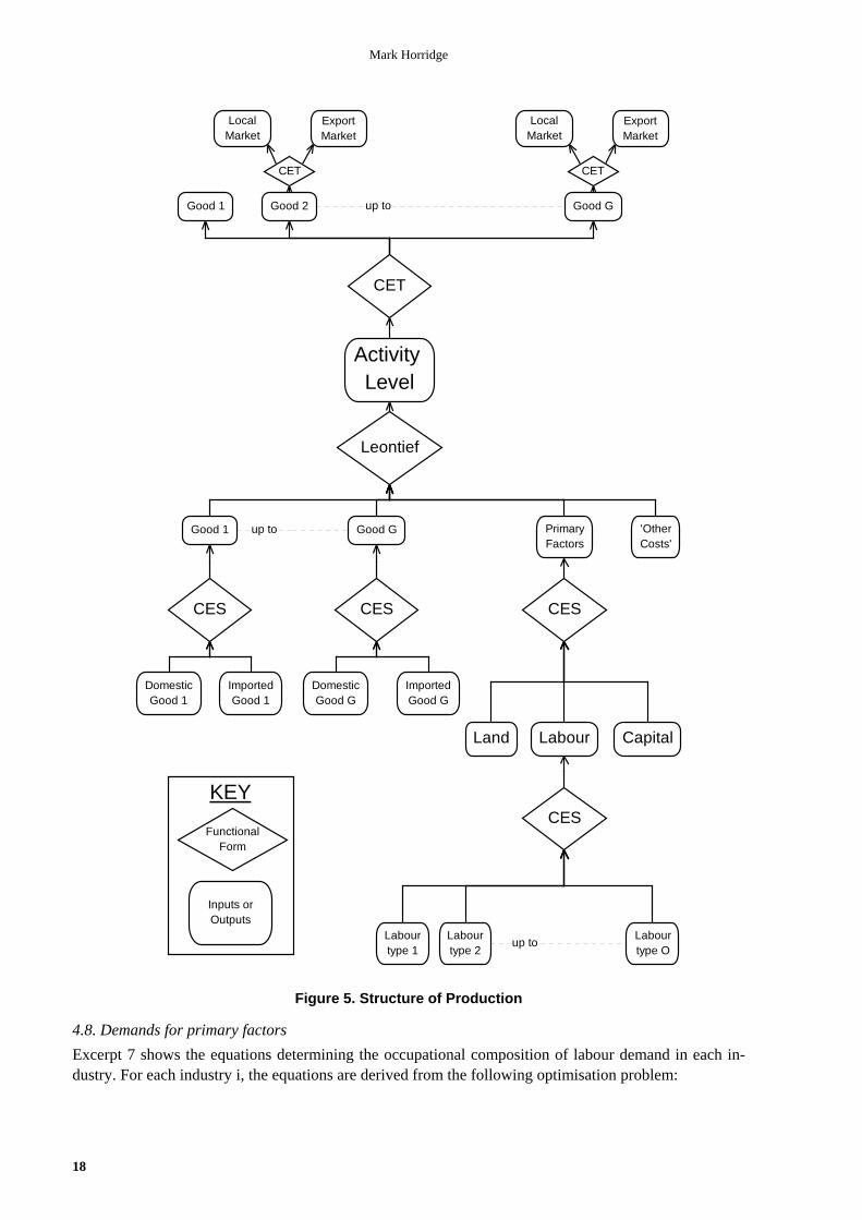
ORANI-G allows each industry to produce several commodities, using as inputs domestic and importedcommodities, labour of several types, land, and capital. In addition, commodities destined for export aredistinguished from those for local use. The multi-input, multi-output production specification is keptmanageable by a series of separability assumptions, illustrated by the nesting shown in Figure 5. Forexample, the assumption of input-output separability implies that the generalised production function forsome industry:
F(inputs,outputs) = 0 (15)
may be written as:
G(inputs) = X1TOT = H(outputs) (16)
where X1TOT is an index of industry activity. Assumptions of this type reduce the number of estimatedparameters required by the model. Figure 5 shows that the H function in (16) is derived from two nestedCET (constant elasticity of transformation) aggregation functions, while the G function is broken into asequence of nests. At the top level, commodity composites, a primary-factor composite and 'other costs'are combined using a Leontief production function. Consequently, they are all demanded in direct pro-portion to X1TOT. Each commodity composite is a CES (constant elasticity of substitution) function of adomestic good and the imported equivalent. The primary-factor composite is a CES aggregate of land,capital and composite labour. Composite labour is a CES aggregate of occupational labour types. Al-though all industries share this common production structure, input proportions and behaviouralparameters may vary between industries.
The nested structure is mirrored in the TABLO equations—each nest requiring 2 sets of equations.We begin at the bottom of Figure 5 and work upwards.
Mark Horridge
18
KEY
Inputs orOutputs
FunctionalForm
CES
CES
CET
Leontief
CESCES
up to
up to
up to
Labourtype O
Labourtype 2
Labourtype 1
Good GGood 2Good 1
CapitalLabourLand
'OtherCosts'
PrimaryFactors
ImportedGood G
DomesticGood G
ImportedGood 1
DomesticGood 1
Good GGood 1
Activity Level
CET
LocalMarket
ExportMarket
CET
LocalMarket
ExportMarket
Figure 5. Structure of Production
4.8. Demands for primary factors
Excerpt 7 shows the equations determining the occupational composition of labour demand in each in-dustry. For each industry i, the equations are derived from the following optimisation problem:

ORANI-G: A Generic Single-Country Computable General Equilibrium Model
19
CES
up toLabourtype O
Labourtype 2
Labourtype 1
Labour
V1LAB(i,o)p1lab(i,o)x1lab(i,o)
V1LAB_O(i)p1lab_o(i)x1lab_o(i)
Boxes showVALUEprice %
quantity %
Figure 6. Demand for different types of labour
Choose inputs of occupation-specific labour,X1LAB(i,o),
to minimize total labour cost,Sum{o,OCC, P1LAB(i,o)*X1LAB(i,o)},
whereX1LAB_O(i) = CES[ All,o,OCC: X1LAB(i,o)],
regarding as exogenous to the problemP1LAB(i,o) and X1LAB_O(i).
Note that the problem is formulated in the levels of the variables. Hence, we have written the variablenames in upper case. The notation CES[ ] represents a CES function defined over the set of variablesenclosed in the square brackets.
! Excerpt 7 of TABLO input file: !! Occupational composition of labour demand !
Coefficient (parameter)(all,i,IND) SIGMA1LAB(i) # CES substitution between skill types #; (all,i,IND) V1LAB_O(i) # Total labour bill in industry i #; TINY # Small number to prevent zerodivides or singular matrix #;Read SIGMA1LAB from file BASEDATA header "SLAB";Formula (all,i,IND) V1LAB_O(i) = sum{o,OCC, V1LAB(i,o)}; TINY = 0.000000000001;Variable (all,i,IND) p1lab_o(i) # Price to each industry of labour composite #; (all,i,IND) x1lab_o(i) # Effective labour input #;Equation E_x1lab # Demand for labour by industry and skill group # (all,i,IND)(all,o,OCC) x1lab(i,o) = x1lab_o(i) ‐ SIGMA1LAB(i)*[p1lab(i,o) ‐ p1lab_o(i)]; E_p1lab_o # Price to each industry of labour composite # (all,i,IND) [TINY+V1LAB_O(i)]*p1lab_o(i) = sum{o,OCC, V1LAB(i,o)*p1lab(i,o)};
The solution of this problem, in percentage-change form, is given by equations E_x1lab andE_p1lab_o (see Appendix A for derivation). The first of the equations indicates that demand for labourtype o is proportional to overall labour demand, X1LAB_O, and to a price term. In change form, theprice term is composed of an elasticity of substitution, SIGMA1LAB(i), multiplied by the percentagechange in a price ratio [p1lab(i,o)-p1lab_o(i)] representing the wage of occupation o relative to the aver-age wage for labour in industry i. Changes in the relative prices of the occupations induce substitution infavour of relatively cheapening occupations. The percentage change in the average wage, p1lab_o(i), isgiven by the second of the equations. This could be rewritten:

Mark Horridge
20
p1lab_o(i) = sum{o,OCC, S1LAB(i,o)*p1lab(i,o)},if S1LAB(i,o) were the value share of occupation o in the total wage bill of industry i. In other words,p1lab_o(i) is a Divisia index of the p1lab(i,o).
It is worth noting that if the individual equations of E_x1lab were multiplied by corresponding ele-ments of S1LAB(i,o), and then summed together, all price terms would disappear, giving:
x1lab_o(i) = sum{o,OCC, S1LAB(i,o)*x1lab(i,o)}.This is the percentage-change form of the CES aggregation function for labour.
For an industry which does not use labour (housing services is a common example), V1LAB(i,o)would contain only zeros so that p1lab_o(i) would be undefined. To prevent this, we add the coefficientTINY (set to some very small number) to the left hand side of equation E_p1lab_o. With V1LAB_O(i)zero, equation E_p1lab_o becomes:
p1lab_o(i) = 0.
The same procedure is used extensively in later equations.
CES
CapitalLabourLand
PrimaryFactors
V1CAP(i)p1cap(i)x1cap(i)
V1PRIM(i)p1prim(i)x1prim(i)
V1LAB_O(i)p1lab_o(i)x1lab_o(i)
V1LND(i)p1lnd(i)x1lnd(i)
Figure 7. Primary Factor Demand
Excerpt 8 contains equations determing the composition of demand for primary factors. Their derivationfollows a pattern similar to that underlying the previous nest. In this case, total primary factor costs areminimised subject to the production function:
X1PRIM(i) = CES[ X1LAB_O(i)A1LAB_O(i)
, X1CAP(i)A1CAP(i)
, X1LND(i)A1LND(i)].
Because we may wish to introduce factor-saving technical changes, we include explicitly the coefficientsA1LAB_O(i), A1CAP(i), and A1LND(i).
The solution to this problem, in percentage-change form, is given by equations E_x1lab_o, E_x1capand E_x1lnd, and E_p1prim. Ignoring the technical-change terms, we see that demand for each factor isproportional to overall factor demand, X1PRIM, and to a price term. In change form the price term is anelasticity of substitution, SIGMA1PRIM(i), multiplied by the percentage change in a price ratio repre-senting the cost of an effective unit of the factor relative to the overall, effective cost of primary factorinputs to industry i. Changes in the relative prices of the primary factors induce substitution in favour ofrelatively cheapening factors. The percentage change in the average effective cost, p1prim(i), given byequation E_p1prim, is again a cost-weighted Divisia index of individual prices and technical changes.

ORANI-G: A Generic Single-Country Computable General Equilibrium Model
21
! Excerpt 8 of TABLO input file: !! Primary factor proportions !
Coefficient(parameter)(all,i,IND) SIGMA1PRIM(i) # CES substitution, primary factors #;Read SIGMA1PRIM from file BASEDATA header "P028";Coefficient (all,i,IND) V1PRIM(i) # Total factor input to industry i#;Formula (all,i,IND) V1PRIM(i) = V1LAB_O(i)+ V1CAP(i) + V1LND(i);Variable (all,i,IND) p1prim(i) # Effective price of primary factor composite #; (all,i,IND) x1prim(i) # Primary factor composite #; (all,i,IND) a1lab_o(i) # Labor‐augmenting technical change #; (all,i,IND) a1cap(i) # Capital‐augmenting technical change #; (all,i,IND) a1lnd(i) # Land‐augmenting technical change #;(change)(all,i,IND) delV1PRIM(i)# Ordinary change in cost of primary factors #;
Equation E_x1lab_o # Industry demands for effective labour # (all,i,IND) x1lab_o(i) ‐ a1lab_o(i) = x1prim(i) ‐ SIGMA1PRIM(i)*[p1lab_o(i) + a1lab_o(i) ‐ p1prim(i)];
E_p1cap # Industry demands for capital # (all,i,IND) x1cap(i) ‐ a1cap(i) = x1prim(i) ‐ SIGMA1PRIM(i)*[p1cap(i) + a1cap(i) ‐ p1prim(i)];
E_p1lnd # Industry demands for land # (all,i,IND) x1lnd(i) ‐ a1lnd(i) = x1prim(i) ‐ SIGMA1PRIM(i)*[p1lnd(i) + a1lnd(i) ‐ p1prim(i)];
E_p1prim # Effective price term for factor demand equations # (all,i,IND) V1PRIM(i)*p1prim(i) = V1LAB_O(i)*[p1lab_o(i) + a1lab_o(i)] + V1CAP(i)*[p1cap(i) + a1cap(i)] + V1LND(i)*[p1lnd(i) + a1lnd(i)];
E_delV1PRIM # Ordinary change in total cost of primary factors # (all,i,IND) 100*delV1PRIM(i) = V1CAP(i) * [p1cap(i) + x1cap(i)] + V1LND(i) * [p1lnd(i) + x1lnd(i)] + sum{o,OCC, V1LAB(i,o)* [p1lab(i,o) + x1lab(i,o)]};
Appendix A contains a formal derivation of CES demand equations with technical-change terms.The technical-change terms appear in a predictable pattern. Imagine that the percentage-change equa-tions lacked these terms, as in the previous, occupational-demand, block. We could add them in by:
replacing each quantity (x) variable by (x-a);replacing each price (p) variable by (p+a); andrearranging terms.
The last equation defines DelV1PRIM, the ordinary change in total cost of primary factors to each in-dustry. This variable is used later in computing industries' total production costs.
4.9. Sourcing of intermediate inputs
We adopt the Armington (1969; 1970) assumption that imports are imperfect substitutes for domesticsupplies. Excerpt 9 shows equations determining the import/domestic composition of intermediate com-modity demands. They follow a pattern similar to the previous nest. Here, the total cost of imported anddomestic good i are minimised subject to the production function:
X1_S(c,i) = CES[All,s,SRC: X1(c,s,i)A1(c,s,i)], (17)

Mark Horridge
22
CESCES
up to
Imported Good C
DomesticGood C
ImportedGood 1
DomesticGood 1
Good CGood 1V1PUR_S(c,i)
p1_s(c,i)x1_s(c,i)
V1PUR(c,s,i)p1(c,s,i)x1(c,s,i)
Boxes showVALUEprice %
quantity %
Figure 8. Intermediate input sourcing decision
Commodity demand from each source is proportional to demand for the composite, X1_S(c,i), and to aprice term. The change form of the price term is an elasticity of substitution, SIGMA1(i), multiplied bythe percentage change in a price ratio representing the effective price from the source relative to theeffective cost of the import/domestic composite. Lowering of a source-specific price, relative to theaverage, induces substitution in favour of that source. The percentage change in the average effectivecost, p1_s(i), is again a cost-weighted Divisia index of individual prices and technical changes.
! Excerpt 9 of TABLO input file: !! Import/domestic composition of intermediate demands !
Variable (all,c,COM)(all,s,SRC)(all,i,IND) a1(c,s,i) # Intermediate basic tech change #; (all,c,COM)(all,i,IND) x1_s(c,i) # Intermediate use of imp/dom composite #; (all,c,COM)(all,i,IND) p1_s(c,i) # Price, intermediate imp/dom composite #; (all,i,IND) p1mat(i) # Intermediate cost price index #; (all,i,IND) p1var(i) # Short‐run variable cost price index #;Coefficient (parameter)(all,c,COM) SIGMA1(c) # Armington elasticities: intermediate #; (all,c,COM)(all,i,IND) V1PUR_S(c,i) # Dom+imp intermediate purch. value #; (all,c,COM)(all,s,SRC)(all,i,IND) S1(c,s,i) # Intermediate source shares #; (all,i,IND) V1MAT(i) # Total intermediate cost for industry i #; (all,i,IND) V1VAR(i) # Short‐run variable cost for industry i #;Read SIGMA1 from file BASEDATA header "1ARM";Zerodivide default 0.5;Formula (all,c,COM)(all,i,IND) V1PUR_S(c,i) = sum{s,SRC, V1PUR(c,s,i)}; (all,c,COM)(all,s,SRC)(all,i,IND) S1(c,s,i) = V1PUR(c,s,i) / V1PUR_S(c,i); (all,i,IND) V1MAT(i) = sum{c,COM, V1PUR_S(c,i)}; (all,i,IND) V1VAR(i) = V1MAT(i) + V1LAB_O(i);Zerodivide off;
Equation E_x1 # Source‐specific commodity demands # (all,c,COM)(all,s,SRC)(all,i,IND) x1(c,s,i)‐a1(c,s,i) = x1_s(c,i) ‐SIGMA1(c)*[p1(c,s,i) +a1(c,s,i) ‐p1_s(c,i)];
Equation E_p1_s # Effective price of commodity composite # (all,c,COM)(all,i,IND) p1_s(c,i) = sum{s,SRC, S1(c,s,i)*[p1(c,s,i) + a1(c,s,i)]};
Equation E_p1mat # Intermediate cost price index # (all,i,IND) p1mat(i) = sum{c,COM, sum{s,SRC, (V1PUR(c,s,i)/ID01[V1MAT(i)])*p1(c,s,i)}};

ORANI-G: A Generic Single-Country Computable General Equilibrium Model
23
Equation E_p1var # Short‐run variable cost price index # (all,i,IND) p1var(i) = [1/V1VAR(i)]*[V1MAT(i)*p1mat(i) + V1LAB_O(i)*p1lab_o(i)];
Following the pattern established for factor demands, we could have written Equation E_p1_s as:
V1PUR_S(c,i)*p1_s(c,i)=Sum{s,SRC,V1PUR(c,s,i)*[p1(c,s,i)+a1(c,s,i)]};
where V1PUR_S(c,i) is the sum over domestic and imported of V1PUR(c,s,i). However, this equationwould have left p1_s(c,i) undefined when V1PUR_S(c,i) is zero—not all industries use all commodities.In computing the share:
S1(c,s,i) =V1PUR(c,s,i)/V1PUR_S(c,i),
(see again Excerpt 9) we used the Zerodivide statement to instruct GEMPACK to set import anddomestic shares (arbitrarily) to 0.5 in such cases. This device avoids a numerical error in computing,without any other substantive consequence.
The last 2 equations defines 2 variables used to explain results. P1mat is an industry-specific indexof the price of intermediate inputs10. P1var is an index of short-run variable cost: it includes the cost ofall industry inputs except capital and land (which are fixed in the short-run). Changes in p1varcorrespond to vertical shifts in shortrun industry supply schedules. Equations for both p1mat and p1varare written with no coefficient on the LHS—this facilitates the use of GEMPACK’s AnalyseGE tool.AnalyseGE is able to ‘decompose’ the RHS of these equations to show the contribution of eachindividual price change to the total change in p1mat or p1var.
4.10. Top production nest
Excerpt 10 covers the topmost input-demand nest of Figure 5. Commodity composites, the primary-factor composite and 'other costs' are combined using a Leontief production function, given by:
X1TOT(i) = 1
A1TOT(i)
MIN[All,c,COM: X1_S(c,i)A1_S(c,i)
, X1PRIM(i)A1PRIM(i)
, X1OCT(i)A1OCT(i)]. (18)
Consequently, each of these three categories of inputs identified at the top level is demanded in directproportion to X1TOT(i).
The Leontief production function is equivalent to a CES production function with the substitutionelasticity set to zero. Hence, the demand equations resemble those derived from the CES case but lackprice (substitution) terms. The a1tot(i) are Hicks-neutral technical-change terms, affecting all inputsequally.
! Excerpt 10 of TABLO input file: !! Top nest of industry input demands !Variable (all,i,IND) x1tot(i) # Activity level or value‐added #; (all,i,IND) a1prim(i) # All factor augmenting technical change #; (all,i,IND) a1tot(i) # All input augmenting technical change #; (all,i,IND) p1tot(i) # Average input/output price #; (all,i,IND) a1oct(i) # "Other cost" ticket augmenting techncal change#; (all,c,COM)(all,i,IND) a1_s(c,i) # Tech change, int'mdiate imp/dom composite #;
Equation E_x1_s # Demands for commodity composites # (all,c,COM)(all,i,IND) x1_s(c,i) ‐ [a1_s(c,i) + a1tot(i)] = x1tot(i);
Equation E_x1prim # Demands for primary factor composite # (all,i,IND) x1prim(i) ‐ [a1prim(i) + a1tot(i)] = x1tot(i);
Equation E_x1oct # Demands for other cost tickets # (all,i,IND) x1oct(i) ‐ [a1oct(i) + a1tot(i)] = x1tot(i);
10 Equation E_p1mat uses the ID01 function built-in to GEMPACK: another way of avoiding divide-by-zeroproblems. If x=0, ID01(x)=1; otherwise ID01(x)=x.

Mark Horridge
24
4.11. Industry costs and production taxes
Excerpt 11 computes levels and changes in the total cost of production both excluding (V1CST) and in-cluding (V1TOT) an ad valorem production tax, V1PTX. The equations are arranged to facilitatechanging the base of the production tax. For example, a comment line underneath equation E_delV1PTXshows how a value-added tax might be implemented: by making V1PRIM (rather than V1CST) the taxbase.
! Excerpt 11 of TABLO input file: !! Output cost inclusive of production tax !
Coefficient (all,i,IND) V1CST(i) # Total cost of industry i #; (all,i,IND) V1TOT(i) # Total industry cost plus tax #; (all,i,IND) PTXRATE(i) # Rate of production tax #;Formula (all,i,IND) V1CST(i) = V1PRIM(i) + V1OCT(i) + V1MAT(i); (all,i,IND) V1TOT(i) = V1CST(i) + V1PTX(i); (all,i,IND) PTXRATE(i) = V1PTX(i)/V1CST(i); !VAT: V1PTX/V1PRIM !Write PTXRATE to file SUMMARY header "PTXR";Variable (change)(all,i,IND) delV1CST(i) # Change in ex‐tax cost of production #; (change)(all,i,IND) delV1TOT(i) # Change in tax‐inc cost of production #; (change)(all,i,IND) delPTXRATE(i) # Change in rate of production tax #;
Equation E_delV1CST (all,i,IND) delV1CST(i) = delV1PRIM(i) + sum{c,COM,sum{s,SRC, 0.01*V1PUR(c,s,i)*[p1(c,s,i) + x1(c,s,i)]}} + 0.01*V1OCT(i) *[p1oct(i) + x1oct(i)];
E_delV1PTX (all,i,IND) delV1PTX(i) = PTXRATE(i)*delV1CST(i) + V1CST(i) * delPTXRATE(i); ! VAT alternative: PTXRATE(i)*delV1PRIM(i) + V1PRIM(i)* delPTXRATE(i); !
E_delV1TOT (all,i,IND) delV1TOT(i) = delV1CST(i) + delV1PTX(i);
E_p1tot (all,i,IND) V1TOT(i)*[p1tot(i) + x1tot(i)] = 100*delV1TOT(i);
Variable (all,i,IND) p1cst(i) # Index of production costs (for AnalyseGE) #;Equation E_p1cst (all,i,IND) p1cst(i) = [1/V1CST(i)]*[ sum{c,COM,sum{s,SRC, V1PUR(c,s,i)*p1(c,s,i)}} + V1OCT(i) *p1oct(i) + V1CAP(i) *p1cap(i) + V1LND(i) *p1lnd(i) + sum{o,OCC, V1LAB(i,o) *p1lab(i,o)}];
The penultimate equation defines p1tot(i) as the percentage change in the unit cost of production forindustry i. Given the constant returns to scale which characterise the model's production technology,p1tot is also the percentage change in marginal cost. We enforce the competitive Zero Pure Profits con-dition (price = marginal cost) by assuming that the p1tot are also equal to the average price received byeach industry.
Under constant returns to scale, we could combine equations listed previously to deduce: p1tot(i) = Skpk + tax and technical change terms
where Sk and pk are respectively the share of input k in total cost, and the percent change in its price.The final equation defines another variable used to explain results. P1cst is an index of production
costs which can be decomposed using AnalyseGE to show the contribution of individual price changesto the total change in input costs. This index ignores the effects of technical change.

ORANI-G: A Generic Single-Country Computable General Equilibrium Model
25
4.12. From industry outputs to commodity ouputs
ORANI-G allows for each industry to produce a mixture of all the commodities. For each industry, themix varies, according to the relative prices of commodities11. The first two equations of Excerpt 12 de-termine the commodity composition of industry output—the final nest of Figure 5. Here, the totalrevenue from all outputs is maximised subject to the production function:
X1TOT(i) = CET[ All,c,COM: Q1(c,i)]. (19)
The CET (constant elasticity of transformation) aggregation function is identical to CES, except that thetransformation parameter in the CET function has the opposite sign to the substitution parameter in theCES function. In equation E_q1, an increase in a commodity price, relative to the average, induces trans-formation in favour of that output. The symbol, p1tot, defined in E_x1tot as average unit revenue, is thesame as that used in the previous equation group to refer to the effective price of a unit of activity. Thisconfirms our interpretation of equation E_p1tot as a Zero Pure Profits condition.
CET
up to Good GGood 2Good 1
Activity Level
CET
LocalMarket
ExportMarket
CET
LocalMarket
ExportMarket
V1TOT(i)p1tot(i)x1tot(i)
One Industry:MAKE(c,i)p0com(c)
q1(c,i)
DOMSALES(c)p0dom(c)x0dom(c)
All-Industry:SALES(c)p0com(c)x0com(c)
V4BAS(c)pe(c)x4(c,i)
Figure 9. Composition of output
Equation E_pq1 states that all industries that produce, say, Cereals, receive the same unit price,p0com("Cereals"). Cereals produced by different industries are deemed to be perfect substitutes12.Equation E_x0com simply adds up all industries' output of each commodity to get the total supply,x0com.
Most non-Australian applications of the ORANI-G framework enforce a one-to-one correspondencebetween industries and commodities This is implied whenever all off-diagonal elements of the MAKEmatrix are zero. In this case, the equations of Excerpt 12 just equate corresponding elements of p0comand p1tot. Similarly, x1tot and x0com become, in effect, the same variable. The computational overheadof including the MAKE mechanism is very slight.
11 Multiproduction can be useful even where each industry produces just one commodity. For example we couldsplit electricity generation into 2 parts: oil-fired and nuclear, each producing the same commodity, electricity.12 The perfect substitute assumption causes problems when we have two industries just producing the samecommodity, and neither industry has a fixed factor; eg, in a long-run closure with mobile capital, and twoelectricity industries (say, nuclear and coal-fired) both making electric power. The model will find it hard to decidewhat proportion of generation should be nuclear. To cover such a case, the TABLO input file contains optionalequations (not shown here), which allow (for example) nuclear electricity to be an imperfect substitute for coal-fired electricity.

Mark Horridge
26
! Excerpt 12 of TABLO input file: !! Output mix of commodities !
Coefficient (all,c,COM)(all,i,IND) MAKE(c,i) # Multiproduction matrix #;Variable (all,c,COM)(all,i,IND) q1(c,i) # Output by commodity and industry #; (all,c,COM)(all,i,IND) pq1(c,i) # Price of com c produced by ind i #; (all,c,COM) p0com(c) # General output price of locally‐produced commodity #;Read MAKE from file BASEDATA header "MAKE";Update (all,c,COM)(all,i,IND) MAKE(c,i)= pq1(c,i)*q1(c,i);Variable (all,c,COM) x0com(c) # Output of commodities #;Coefficient (parameter)(all,i,IND) SIGMA1OUT(i) # CET transformation elasticities #;Read SIGMA1OUT from file BASEDATA header "SCET";Equation E_q1 # Supplies of commodities by industries # (all,c,COM)(all,i,IND) q1(c,i) = x1tot(i) + SIGMA1OUT(i)*[p0com(c) ‐ p1tot(i)];Coefficient (all,i,IND) MAKE_C(i) # All production by industry i #; (all,c,COM) MAKE_I(c) # Total production of commodities #;Formula (all,i,IND) MAKE_C(i) = sum{c,COM, MAKE(c,i)}; (all,c,COM) MAKE_I(c) = sum{i,IND, MAKE(c,i)};
Equation E_x1tot # Average price received by industries # (all,i,IND) p1tot(i) = sum{c,COM, [MAKE(c,i)/MAKE_C(i)]*pq1(c,i)};
Equation E_pq1 # Each industry gets the same price for a given commodity # (all,c,COM)(all,i,IND) pq1(c,i) = p0com(c); E_x0com # Total output of commodities (as simple addition) # (all,c,COM) x0com(c) = sum{i,IND, [MAKE(c,i)/MAKE_I(c)]*q1(c,i)};
4.13. Export and local market versions of each good
Excerpt 13 allows for the possibility that goods destined for export are not the the same as those for localuse13. Conversion of an undifferentiated commodity into goods for both destinations is governed by aCET transformation frontier. Conceptually, the system is the same as Excerpt 12, but it is expressed alittle differently; partly because there are only two outputs; and partly to facilitate switching the systemoff. This is achieved by setting TAU to zero, so that p0com, p0dom and pe are all equal.
! Excerpt 13 of TABLO input file: !! CET between outputs for local and export markets !Variable (all,c,COM) x0dom(c) # Output of commodities for local market #;Coefficient (all, c,COM) EXPSHR(c) # Share going to exports #; (all, c,COM) TAU(c) # 1/Elast. of transformation, exportable/locally used #;Zerodivide default 0.5;Formula (all,c,COM) EXPSHR(c) = V4BAS(c)/MAKE_I(c); (all,c,COM) TAU(c) = 0.0; ! if zero, p0dom = pe, and CET is nullified !Zerodivide off;Equation E_x0dom # Supply of commodities to export market # (all,c,COM) TAU(c)*[x0dom(c) ‐ x4(c)] = p0dom(c) ‐ pe(c);Equation E_pe # Supply of commodities to domestic market # (all,c,COM) x0com(c) = [1.0‐EXPSHR(c)]*x0dom(c) + EXPSHR(c)*x4(c);Equation E_p0com # Zero pure profits in transformation # (all,c,COM) p0com(c) = [1.0‐EXPSHR(c)]*p0dom(c) + EXPSHR(c)*pe(c);
13 This feature is not part of the ORANI tradition, but appears in some other applied GE models.

ORANI-G: A Generic Single-Country Computable General Equilibrium Model
27
The names of the prices, quantities and flows in the two CET nests of Excerpt 12 are shown below:
Joint Production CET NestType ofVariable
IndustryOutput
CommodityOutputs
UndifferentiatedCommodity
LocalDestination
ExportDestination
% quantity x1tot(i) q1(c,i) x0com(c) x0dom(c) x4(c)% price p1tot(i) p0com(c) p0com(c) p0dom(c) =
p0(c,”dom”)pe(c)
Value of flow V1TOT(i) MAKE(c,i) SALES(c) DOMSALES(c) V4BAS(c)Export/Domestic CET nest
Note that V1TOT(i) = cMAKE(c,i) and SALES(c) = iMAKE(c,i) = DOMSALES(c) + V4BAS(c)
4.14. Demands for investment goods
Figure 10 shows the nesting structure for the production of new units of fixed capital. Capital is assumedto be produced with inputs of domestically produced and imported commodities. The productionfunction has the same nested structure as that which governs intermediate inputs to current production.No primary factors are used directly as inputs to capital formation.
Leontief
CESCES
up to
Imported Good C
DomesticGood C
ImportedGood 1
DomesticGood 1
Good CGood 1
New Capitalfor Industry i
V2TOT(i)p2tot(i)x2tot(i)
V2PUR_S(c,i)p2_s(c,i)x2_s(c,i)
V2PUR(c,s,i)p2(c,s,i)x2(c,s,i)
Figure 10. Structure of Investment Demand
The investment demand equations (see Excerpt 14) are derived from the solutions to the investor'stwo-part cost-minimisation problem. At the bottom level, the total cost of imported and domestic good iis minimised subject to the CES production function:
X2_S(c, i) = CES[All,s,SRC: X2(c,s,i)A2(c,s,i)], (20)
while at the top level the total cost of commodity composites is minimised subject to the Leontief pro-duction function:
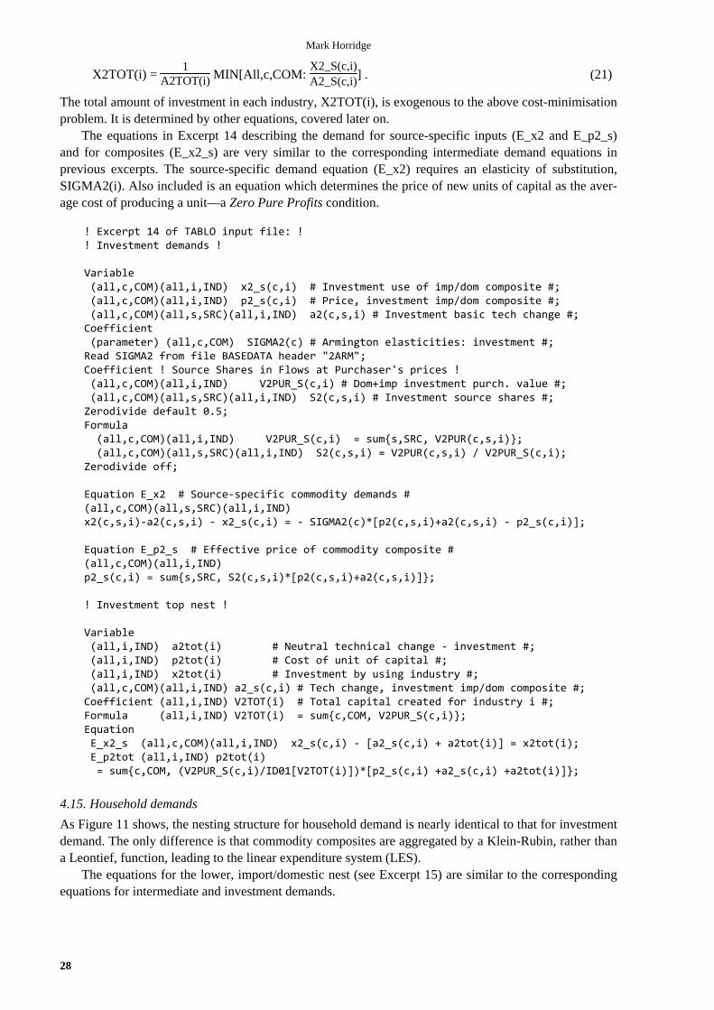
Mark Horridge
28
X2TOT(i) = 1
A2TOT(i) MIN[All,c,COM:X2_S(c,i)A2_S(c,i)] . (21)
The total amount of investment in each industry, X2TOT(i), is exogenous to the above cost-minimisationproblem. It is determined by other equations, covered later on.
The equations in Excerpt 14 describing the demand for source-specific inputs (E_x2 and E_p2_s)and for composites (E_x2_s) are very similar to the corresponding intermediate demand equations inprevious excerpts. The source-specific demand equation (E_x2) requires an elasticity of substitution,SIGMA2(i). Also included is an equation which determines the price of new units of capital as the aver-age cost of producing a unit—a Zero Pure Profits condition.
! Excerpt 14 of TABLO input file: !! Investment demands !
Variable (all,c,COM)(all,i,IND) x2_s(c,i) # Investment use of imp/dom composite #; (all,c,COM)(all,i,IND) p2_s(c,i) # Price, investment imp/dom composite #; (all,c,COM)(all,s,SRC)(all,i,IND) a2(c,s,i) # Investment basic tech change #;Coefficient (parameter) (all,c,COM) SIGMA2(c) # Armington elasticities: investment #;Read SIGMA2 from file BASEDATA header "2ARM";Coefficient ! Source Shares in Flows at Purchaser's prices ! (all,c,COM)(all,i,IND) V2PUR_S(c,i) # Dom+imp investment purch. value #; (all,c,COM)(all,s,SRC)(all,i,IND) S2(c,s,i) # Investment source shares #;Zerodivide default 0.5;Formula (all,c,COM)(all,i,IND) V2PUR_S(c,i) = sum{s,SRC, V2PUR(c,s,i)}; (all,c,COM)(all,s,SRC)(all,i,IND) S2(c,s,i) = V2PUR(c,s,i) / V2PUR_S(c,i);Zerodivide off;
Equation E_x2 # Source‐specific commodity demands #(all,c,COM)(all,s,SRC)(all,i,IND)x2(c,s,i)‐a2(c,s,i) ‐ x2_s(c,i) = ‐ SIGMA2(c)*[p2(c,s,i)+a2(c,s,i) ‐ p2_s(c,i)];
Equation E_p2_s # Effective price of commodity composite #(all,c,COM)(all,i,IND)p2_s(c,i) = sum{s,SRC, S2(c,s,i)*[p2(c,s,i)+a2(c,s,i)]};
! Investment top nest !
Variable (all,i,IND) a2tot(i) # Neutral technical change ‐ investment #; (all,i,IND) p2tot(i) # Cost of unit of capital #; (all,i,IND) x2tot(i) # Investment by using industry #; (all,c,COM)(all,i,IND) a2_s(c,i) # Tech change, investment imp/dom composite #;Coefficient (all,i,IND) V2TOT(i) # Total capital created for industry i #;Formula (all,i,IND) V2TOT(i) = sum{c,COM, V2PUR_S(c,i)};Equation E_x2_s (all,c,COM)(all,i,IND) x2_s(c,i) ‐ [a2_s(c,i) + a2tot(i)] = x2tot(i); E_p2tot (all,i,IND) p2tot(i) = sum{c,COM, (V2PUR_S(c,i)/ID01[V2TOT(i)])*[p2_s(c,i) +a2_s(c,i) +a2tot(i)]};
4.15. Household demands
As Figure 11 shows, the nesting structure for household demand is nearly identical to that for investmentdemand. The only difference is that commodity composites are aggregated by a Klein-Rubin, rather thana Leontief, function, leading to the linear expenditure system (LES).
The equations for the lower, import/domestic nest (see Excerpt 15) are similar to the correspondingequations for intermediate and investment demands.

ORANI-G: A Generic Single-Country Computable General Equilibrium Model
29
Klein-Rubin
CESCES
up to
Imported Good C
DomesticGood C
ImportedGood 1
Domestic Good 1
Good CGood 1
Household Utility
V3TOTp3totx3tot
V3PUR(c,s)p3(c,s)x3(c,s)
3t t
V3PUR_S(c)p3_s(c)x3_s(c)
3t t
SubsistenceV3SUB(c)
p3_s(c)x3sub(c)
3t t
LuxuryV3LUX(c)p3_s(c)x3lux(c)
3t t
Figure 11. Structure of Consumer Demand
! Excerpt 15 of TABLO input file: !! Import/domestic composition of household demands !
Variable(all,c,COM)(all,s,SRC) a3(c,s) # Household basic taste change #;(all,c,COM) x3_s(c) # Household use of imp/dom composite #;(all,c,COM) p3_s(c) # Price, household imp/dom composite #;Coefficient (parameter)(all,c,COM) SIGMA3(c) # Armington elasticities: households #;Read SIGMA3 from file BASEDATA header "3ARM";
Coefficient ! Source Shares in Flows at Purchaser's prices ! (all,c,COM) V3PUR_S(c) # Dom+imp households purch. value #; (all,c,COM)(all,s,SRC) S3(c,s) # Household source shares #;Zerodivide default 0.5;Formula (all,c,COM) V3PUR_S(c) = sum{s,SRC, V3PUR(c,s)}; (all,c,COM)(all,s,SRC) S3(c,s) = V3PUR(c,s) / V3PUR_S(c);Zerodivide off;
Equation E_x3 # Source‐specific commodity demands #(all,c,COM)(all,s,SRC)x3(c,s)‐a3(c,s) = x3_s(c) ‐ SIGMA3(c)*[ p3(c,s)+a3(c,s) ‐ p3_s(c) ];
Equation E_p3_s # Effective price of commodity composite #(all,c,COM) p3_s(c) = sum{s,SRC, S3(c,s)*[p3(c,s)+a3(c,s)]};

Mark Horridge
30
Excerpt 16 of the TABLO input file determines the allocation of household expenditure betweencommodity composites. This is derived from the Klein-Rubin utility function:
Utility per household = 1Qc
{X3_S(c) - X3SUB(c)}S3LUX(c), (22)
The X3SUB and S3LUX are behavioural coefficients—the S3LUX must sum to unity. Q is the numberof households. The demand equations that arise from this utility function are:
X3_S(c) = X3SUB(c) + S3LUX(c)*V3LUX_C/P3_S(c), (23)
where:
V3LUX_C = V3TOT - X3SUB(c)*P3_S(c) (24)
The name of the linear expenditure system derives from its property that expenditure on each good isa linear function of prices (P3_S) and expenditure (V3TOT). The form of the demand equations givesrise to the following interpretation. The X3SUB are said to be the 'subsistence' requirements of eachgood—these quantities are purchased regardless of price. V3LUX_C is what remains of the consumerbudget after subsistence expenditures are deducted—we call this 'luxury' or 'supernumerary' expenditure.The S3LUX are the shares of this remnant allocated to each good—the marginal budget shares. Such aninterpretation facilitates our transition to percentage change form, which begins from the levels equa-tions:
X3_S(c) = X3SUB(c) + X3LUX(c) (25)
X3LUX(c)*P3_S(c) = S3LUX(c)*V3LUX_C (26)
X3SUB(c) = Q*A3SUB(c) (27)
As equation (25) makes plain, the X3LUX are luxury usages, or the difference between the subsistencequantities and total demands. Equation (26) states that luxury expenditures follow the marginal budgetshares S3LUX. Together, equations (25) and (26) are equivalent to (23). Equation (27) is necessary be-cause our demand system applies to aggregate instead of to individual households. It states that totalsubsistence demand for each good c is proportional to the number of households, Q, and to the individualhousehold subsistence demands, A3SUB(c). The percentage change forms of equations (27), (26) and(25) appear as the first three items in Excerpt 16 of the Tablo Input File. Note that a3lux(c) and w3luxare respectively the percentage changes in S3LUX(c) and V3LUX_C.
! Excerpt 16 of TABLO input file: !! Household demands for composite commodities !Variable p3tot # Consumer price index #; x3tot # Real household consumption #; w3lux # Total nominal supernumerary household expenditure #; w3tot # Nominal total household consumption #; q # Number of households #; utility # Utility per household #; (all,c,COM) x3lux(c) # Household ‐ supernumerary demands #; (all,c,COM) x3sub(c) # Household ‐ subsistence demands #; (all,c,COM) a3lux(c) # Taste change, supernumerary demands #; (all,c,COM) a3sub(c) # Taste change, subsistence demands #; (all,c,COM) a3_s(c) # Taste change, household imp/dom composite #;Coefficient V3TOT # Total purchases by households #; FRISCH # Frisch LES 'parameter'= ‐ (total/luxury) #; (all,c,COM) EPS(c) # Household expenditure elasticities #; (all,c,COM) S3_S(c) # Household average budget shares #; (all,c,COM) B3LUX(c) # Ratio, (supernumerary expenditure/total expenditure) #; (all,c,COM) S3LUX(c) # Marginal household budget shares #;Read FRISCH from file BASEDATA header "P021"; EPS from file BASEDATA header "XPEL";Update (change) FRISCH = FRISCH*[w3tot ‐ w3lux]/100.0; (change)(all,c,COM) EPS(c) = EPS(c)*[x3lux(c)‐x3_s(c)+w3tot‐w3lux]/100.0;

ORANI-G: A Generic Single-Country Computable General Equilibrium Model
31
Formula V3TOT = sum{c,COM, V3PUR_S(c)}; (all,c,COM) S3_S(c) = V3PUR_S(c)/V3TOT; (all,c,COM) B3LUX(c) = EPS(c)/ABS[FRISCH]; ! initial sign of Frisch ignored ! (all,c,COM) S3LUX(c) = EPS(c)*S3_S(c);Write S3LUX to file SUMMARY header "LSHR"; S3_S to file SUMMARY header "CSHR";Equation E_x3sub # Subsistence demand for composite commodities # (all,c,COM) x3sub(c) = q + a3sub(c);
E_x3lux # Luxury demand for composite commodities # (all,c,COM) x3lux(c) + p3_s(c) = w3lux + a3lux(c);
E_x3_s # Total household demand for composite commodities # (all,c,COM) x3_s(c) = B3LUX(c)*x3lux(c) + [1‐B3LUX(c)]*x3sub(c);
E_utility # Change in utility disregarding taste change terms # utility + q = sum{c,COM, S3LUX(c)*x3lux(c)};
E_a3lux # Default setting for luxury taste shifter # (all,c,COM) a3lux(c) = a3sub(c) ‐ sum{k,COM, S3LUX(k)*a3sub(k)};
E_a3sub # Default setting for subsistence taste shifter # (all,c,COM) a3sub(c) = a3_s(c) ‐ sum{k,COM, S3_S(k)*a3_s(k)};
E_x3tot # Real consumption # x3tot = sum{c,COM, sum{s,SRC, [V3PUR(c,s)/V3TOT]*x3(c,s)}};
E_p3tot # Consumer price index # p3tot = sum{c,COM, sum{s,SRC, [V3PUR(c,s)/V3TOT]*p3(c,s)}};
E_w3tot # Household budget constraint: determines w3lux # w3tot = x3tot + p3tot;
Equation E_utility is the percentage-change form of the utility function (22). Equations E_a3sub andE_a3lux provide default settings for the taste-change variables, a3sub and a3lux, which allow the aver-age budget shares to be shocked, via the a3_s, in a way that preserves the pattern of expenditureelasticities. See Appendix F for further details.
The equations just described determine the composition of household demands but do not determinetotal consumption. That could be done in a variety of ways: (i) set exogenously, (ii) determined by aconsumption funcntion, or (iii) determined via a balance of trade constraint.
The reader may wonder why there is no equation based on (24) which would determine the variablew3lux. The reason is that (24) can be deduced from (23) and the definition of V3TOT:
V3TOT = X3_S(c)*P3_S(c) (28)
The percentage change form of (28) in fact appears as the final equation E_w3tot. Hence any addi-tional equation defining w3lux would be redundant.
4.16. Export demands
To model export demands, commodities in ORANI-G are divided into two groups: For an individual export commodity, foreign demand is inversely related to that commodity's price. For the remaining, collective export, commodities, foreign demand is inversely related to the average
price of all collective export commodities.

Mark Horridge
32
! Excerpt 17 of TABLO input file: !! Export demands !
Coefficient (parameter)(all,c,COM) IsIndivExp(c) # >0.5 For individual export commodities#;Read IsIndivExp from file BASEDATA header "ITEX";! This way of defining a set facilitates aggregation of the data base !Set TRADEXP # Individual export commodities # = (all,c,COM: IsIndivExp(c)>0.5);Write (Set) TRADEXP to file SUMMARY header "TEXP";
Variable phi # Exchange rate, local currency/$world #; (all,c,COM) f4p(c) # Price (upward) shift in export demand schedule #; (all,c,COM) f4q(c) # Quantity (right) shift in export demands #;Coefficient (parameter)(all,c,COM) EXP_ELAST(c) # Export demand elasticities: typical value ‐5.0 #;Read EXP_ELAST from file BASEDATA header "P018";Equation E_x4A # Individual export demand functions #(all,c,TRADEXP) x4(c) ‐ f4q(c) = ‐ABS[EXP_ELAST(c)]*[p4(c) ‐ phi ‐ f4p(c)];! note: ABS function above fixes common mistake: positive EXP_ELAST values !
Set NTRADEXP # Collective Export Commodities # = COM ‐ TRADEXP;Write (Set) NTRADEXP to file SUMMARY header "NTXP";Variable x4_ntrad # Quantity, collective export aggregate #; f4p_ntrad # Upward demand shift, collective export aggregate #; f4q_ntrad # Right demand shift, collective export aggregate #; p4_ntrad # Price, collective export aggregate #;
Coefficient V4NTRADEXP # Total collective export earnings #;Formula V4NTRADEXP = sum{c,NTRADEXP, V4PUR(c)};
Equation E_X4B # Collective export demand functions # (all,c,NTRADEXP) x4(c) ‐ f4q(c) = x4_ntrad;
Equation E_p4_ntrad # Average price of collective exports # [TINY+V4NTRADEXP]*p4_ntrad = sum{c,NTRADEXP, V4PUR(c)*p4(c)};
Coefficient (parameter) EXP_ELAST_NT # Collective export demand elasticity #;Read EXP_ELAST_NT from file BASEDATA header "EXNT";Equation E_x4_ntrad # Demand for collective export aggregate # x4_ntrad ‐ f4q_ntrad = ‐ABS[EXP_ELAST_NT]*[p4_ntrad ‐ phi ‐ f4p_ntrad];
The individual export group, which would normally include all the main export commodities, is definedby the set TRADEXP14 in Excerpt 17. Equation E_x4A specifies downward-sloping foreign demandschedules for these commodities. In the levels, the equation would read:
X4(c) = F4Q(c)[ P4(c)PHI*F4P(c)]
EXP_ELAST(c), (29)
where EXP_ELAST(c) is a negative15 parameter—the constant elasticity of demand. That is, export vol-umes, X4(c), are declining functions of their prices in foreign currency, (P4(c)/PHI). The exchange ratePHI converts local to foreign currency units. The variables F4Q(i) and F4P(i) allow for horizontal(quantity) and vertical (price) shifts in the demand schedules.
The collective export group, defined by the set NTRADEXP, could include all those commoditiesfor which the above equation is inappropriate. For models based on ORANI-G this has typically includedthe bulk of the service commodities, and other commodities (examples might be Air Transport or Gold)
14 The original version of ORANI referred to individual exports as traditional exports; the rest were called non-tra-ditional exports. For Australia, the traditional exports were all primary products.15 The ABS (absolute value) function is used to neutralize mistakes about the sign of EXP_ELAST.

ORANI-G: A Generic Single-Country Computable General Equilibrium Model
33
where export volumes do not seem to depend mainly on the corresponding price. The list would becountry-specific.
The commodity composition of aggregate collective exports is exogenised by treating collectiveexports as a Leontief aggregate (see equation E_x4B). Demand for the aggregate is related to its averageprice via a constant-elasticity demand curve, similar to those for individual exports (see equationE_x4_ntrad).
It is permissible for the set TRADEXP to contain all commodities, so that the set NTRADEXP isempty. This disactivates the collective export mechanism. In addition, exports of particular commoditiesmay be fixed or shocked by exogenising the corresponding elements of the vector x4, while at the sametime endogenising matching elements of the vector f4q.
4.17. Other final demands
Equations E_x5 and E_f5tot determine government usage. With both of the shift variables f5 and f5totexogenous, the level and composition of government consumption is exogenously determined. Thenequation E_f5tot merely determines the value of the endogenous variable f5tot2, which appears nowhereelse. Alternatively, many ORANI applications have assumed that, in the absence of shocks to the shiftvariables, aggregate government consumption moves with real aggregate household consumption, x3tot.This is achieved by endogenising f5tot and exogenising f5tot2. The trick of changing behaviouralspecifications by switching the exogenous/endogenous status of shift variables is used frequently inapplying ORANI. It helps to avoid proliferation of model variants, allowing the same TABLO Input fileto contain different versions of some equations. The choice of which shift variables are exogenous de-termines at run time which version is operative in the rest of the model.
! Excerpt 18 of TABLO input file: !! Government and inventory demands !Variable f5tot # Overall shift term for government demands #; f5tot2 # Ratio between f5tot and x3tot #; (all,c,COM)(all,s,SRC) f5(c,s) # Government demand shift #; (change) (all,c,COM)(all,s,SRC) fx6(c,s) # Shifter on rule for stocks #;Equation E_x5 # Government demands # (all,c,COM)(all,s,SRC) x5(c,s) = f5(c,s) + f5tot; E_f5tot # Overall government demands shift # f5tot = x3tot + f5tot2;
Coefficient (all,c,COM)(all,s,SRC) LEVP0(c,s) # Levels basic prices #;Formula (initial) (all,c,COM)(all,s,SRC) LEVP0(c,s) = 1; ! arbitrary setting !Update (all,c,COM)(all,s,SRC) LEVP0(c,s) = p0(c,s);Equation E_delx6 # Stocks follow domestic output # (all,c,COM)(all,s,SRC) 100*LEVP0(c,s)*delx6(c,s) = V6BAS(c,s)*x0com(c) + fx6(c,s); E_delV6 # Update formula for stocks # (all,c,COM)(all,s,SRC) delV6(c,s) = 0.01*V6BAS(c,s)*p0(c,s) + LEVP0(c,s)*delx6(c,s);
Equation E_delx6 shows one way that delx6, the change in the volume of goods going to invento-ries, might be endogenized. It states that the percentage change in the volume of each commodity,domestic or imported, going to inventories, is the same as the percentage change in domestic productionof that commodity. Like the previous equation, E_delx6 can be insulated from the rest of the equationsystem—by leaving fx6 endogenous. A chief purpose for this equation is to facilitate the real homoge-neity test described in Appendix I.
Equation E_delV6 defines ordinary changes in the values of inventory demands. These are usedabove to update the V6BAS coefficient. The form of the equation arises because delx6 is an ordinary(rather than percentage) change variable. It may be derived by:
V = P.X(PP +
XX ) = V p
100 + PX. (30)
Notice that we are now required to define and update the levels price, P, i.e., we are obliged to specifyunits of measurement for quantities. In the TABLO code the coefficient LEVP0 contains current basic

Mark Horridge
34
prices. The initial values of its elements are set (arbitrarily) to 1 via an earlier 'Formula (Initial)' state-ment. Thus, the unit of measurement of delx6 is base-period-dollars-worth.
4.18. Demands for margins
The equations in Excerpt 19 indicate that, in the absence of technical change, demands for margins areproportional to the commodity flows with which the margins are associated. The 'a' variables allow fortechnical change in margins usage.
! Excerpt 19 of TABLO input file: !! Margin demands !
Variable (all,c,COM)(all,s,SRC)(all,i,IND)(all,m,MAR) a1mar(c,s,i,m) # Intermediate margin tech change #; (all,c,COM)(all,s,SRC)(all,i,IND)(all,m,MAR) a2mar(c,s,i,m) # Investment margin tech change #; (all,c,COM)(all,s,SRC)(all,m,MAR) a3mar(c,s,m) # Household margin tech change#; (all,c,COM)(all,m,MAR) a4mar(c,m) # Export margin tech change #; (all,c,COM)(all,s,SRC)(all,m,MAR) a5mar(c,s,m) # Governmnt margin tech change#;
Equation E_x1mar # Margins to producers # (all,c,COM)(all,s,SRC)(all,i,IND)(all,m,MAR) x1mar(c,s,i,m) = x1(c,s,i) + a1mar(c,s,i,m); E_x2mar # Margins to investment # (all,c,COM)(all,s,SRC)(all,i,IND)(all,m,MAR) x2mar(c,s,i,m) = x2(c,s,i) + a2mar(c,s,i,m); E_x3mar # Margins to households # (all,c,COM)(all,s,SRC)(all,m,MAR) x3mar(c,s,m) = x3(c,s) + a3mar(c,s,m); E_x4mar # Margins to exports # (all,c,COM)(all,m,MAR) x4mar(c,m) = x4(c) + a4mar(c,m); E_x5mar # Margins to government # (all,c,COM)(all,s,SRC)(all,m,MAR) x5mar(c,s,m) = x5(c,s) + a5mar(c,s,m);
4.19. Formulae for sales aggregates
The next two excerpts are concerned with computing aggregate demands for domestic and importedcommodities. Excerpt 20 contains coefficients and formulae for these demands. The aggregate SALEmatrix breaks down demand for domestic and imported goods, valued at basic prices, by their main des-tinations. This is written to the SUMMARY file for later use in analysing results. Note that margin use isidentified separately.
The V0IMP, SALES and DOMSALES aggregates are simply subtotals of the SALE matrix.
! Excerpt 20 of TABLO input file: !! Sales Aggregates !
Coefficient (all,c,COM) MARSALES(c) # Total usage for margins purposes #;Formula (all,n,NONMAR) MARSALES(n) = 0.0; (all,m,MAR) MARSALES(m) = sum{c,COM, V4MAR(c,m) + sum{s,SRC, V3MAR(c,s,m) + V5MAR(c,s,m) + sum{i,IND, V1MAR(c,s,i,m) + V2MAR(c,s,i,m)}}};
Set DEST # Sale Categories #(Interm, Invest, HouseH, Export, GovGE, Stocks, Margins);
Coefficient (all,c,COM)(all,s,SRC)(all,d,DEST) SALE(c,s,d) # Sales aggregates #;Formula (all,c,COM)(all,s,SRC) SALE(c,s,"Interm") = sum{i,IND, V1BAS(c,s,i)}; (all,c,COM)(all,s,SRC) SALE(c,s,"Invest") = sum{i,IND, V2BAS(c,s,i)}; (all,c,COM)(all,s,SRC) SALE(c,s,"HouseH") = V3BAS(c,s); (all,c,COM) SALE(c,"dom","Export") = V4BAS(c); (all,c,COM) SALE(c,"imp","Export") = 0; (all,c,COM)(all,s,SRC) SALE(c,s,"GovGE") = V5BAS(c,s);

ORANI-G: A Generic Single-Country Computable General Equilibrium Model
35
(all,c,COM)(all,s,SRC) SALE(c,s,"Stocks") = V6BAS(c,s); (all,c,COM) SALE(c,"dom","Margins") = MARSALES(c); (all,c,COM) SALE(c,"imp","Margins") = 0;Write SALE to file SUMMARY header "SALE";
Coefficient (all,c,COM) V0IMP(c) # Total basic‐value imports of good c #;Formula (all,c,COM) V0IMP(c) = sum{d,DEST, SALE(c,"imp",d)};Coefficient (all,c,COM) SALES(c) # Total sales of domestic commodities #;Formula (all,c,COM) SALES(c) = sum{d,DEST, SALE(c,"dom",d)};Coefficient (all,c,COM) DOMSALES(c) # Total sales to local market #;Formula (all,c,COM) DOMSALES(c) = SALES(c) ‐ V4BAS(c);
4.20. Market-clearing equations
Excerpt 21 includes market-clearing equations for locally-consumed commodities, both domestic andimported. It begins by defining equations for the delSale matrix variable, which corresponds to theSALE coefficient just described. Each element of delSale shows the ordinary change in a quantity,measured in current prices. This is seen most clearly in the inventory (stocks) terms. The other right handside terms have the form:
V.x/100 = P.X.x/100 = Px
Having constructed delSale, the next two equations are rather simple. E_p0A just adds up all non-exportdemand for domestic commodities: the sum is equal to the previously defined supply variable, x0dom.Similarly, E_x0imp computes the total demand for imports. By exogenously setting the world price ofimports, pf0cif(c), we assume infinite elasticity of the supply of imports.
! Excerpt 21 of TABLO input file: !! Market clearing equations !
Variable (change) (all,c,COM)(all,s,SRC)(all,d,DEST) delSale(c,s,d) # Sales aggregates #;EquationE_delSaleA (all,c,COM)(all,s,SRC) delSale(c,s,"Interm") = 0.01*sum{i,IND,V1BAS(c,s,i)*x1(c,s,i)};E_delSaleB (all,c,COM)(all,s,SRC) delSale(c,s,"Invest") = 0.01*sum{i,IND,V2BAS(c,s,i)*x2(c,s,i)};E_delSaleC (all,c,COM)(all,s,SRC) delSale(c,s,"HouseH")=0.01*V3BAS(c,s)*x3(c,s);E_delSaleD (all,c,COM) delSale(c,"dom","Export")=0.01*V4BAS(c)*x4(c);E_delSaleE (all,c,COM) delSale(c,"imp","Export")= 0;E_delSaleF (all,c,COM)(all,s,SRC) delSale(c,s,"GovGE") =0.01*V5BAS(c,s)*x5(c,s);E_delSaleG (all,c,COM)(all,s,SRC) delSale(c,s,"Stocks") = LEVP0(c,s)*delx6(c,s);E_delSaleH (all,m,MAR) delSale(m,"dom","Margins") = 0.01* sum{c,COM, V4MAR(c,m)*x4mar(c,m) ! note nesting of sum parentheses ! + sum{s,SRC, V3MAR(c,s,m)*x3mar(c,s,m) + V5MAR(c,s,m)*x5mar(c,s,m) + sum{i,IND, V1MAR(c,s,i,m)*x1mar(c,s,i,m) + V2MAR(c,s,i,m)*x2mar(c,s,i,m)}}};E_delSaleI (all,n,NONMAR) delSale(n,"dom","Margins") = 0;E_delSaleJ (all,c,COM) delSale(c,"imp","Margins") = 0;
Set LOCUSER # Non‐export users #(Interm, Invest, HouseH, GovGE, Stocks,Margins);Subset LOCUSER is subset of DEST;
Equation E_p0A # Supply = Demand for domestic commodities #(all,c,COM) 0.01*[TINY+DOMSALES(c)]*x0dom(c) =sum{u,LOCUSER,delSale(c,"dom",u)};
Variable (all,c,COM) x0imp(c) # Total supplies of imported goods #;Equation E_x0imp # Import volumes # (all,c,COM) 0.01*[TINY+V0IMP(c)]*x0imp(c) = sum{u,LOCUSER,delSale(c,"imp",u)};
4.21. Purchasers' prices
The equations in Excerpt 22 define purchasers' prices for each of the first five user groups: producers;investors; households; exports; and government. Purchasers' prices (in levels) are the sums of basic

Mark Horridge
36
values, sales taxes and margins. Sales taxes are treated as ad valorem on basic values, with the sales-taxvariables t in the linearised model being percentage changes in the powers of taxes (The power of a tax isone plus the ad valorem rate). For example, equation E_p3 is derived from the levels form:
X3(c,s)*P3(c,s) = X3(c,s)*P0(c,s)*T3(c,s)
+ sum{m,MAR, X3MAR(c,s,m)*P0(m,"dom") }.
In percentage-change form this is:
V3PUR(c,s)*{x3(c,s) + p3(c,s)} =
{V3TAX(c,s)+V3BAS(c,s)}*{x3(c,s)+p0(c,s)+t3(c,s)}
+ sum{m, MAR, V3MAR(c,s,m)*[x3mar(c,s,m)+p0(m,"dom")]}.
By using Equation E_x3mar from Excerpt 19 to eliminate x3mar(c,s,m), we can cancel out the x3(c,s)terms to obtain:
V3PUR(c,s)*p3(c,s) =
[V3BAS(c,s)+V3TAX(c,s)]*[p0(c,s)+ t3(c,s)] + sum{m,MAR, V3MAR(c,s,m)*[p0(m,"dom")+a3mar(c,s,m)]}.
For a commodity which is not used by households, V3PUR(c,s) and its constituents would all be zero,leaving p3(i,s) undefined. To finesse this problem, the TABLO file adds the coefficient TINY toV3PUR(c,s) so that if it is zero, equation E_p3 becomes:
p3(c,s) = 0.
The same procedure is used for the purchasers'-price equations referring to intermediate, investment, ex-port and government users.
The comment at the end shows how the final equation would appear if the t5 variable (% change inpower) was replaced by delt5: an ordinary change in the ad valorem rate.
! Excerpt 22 of TABLO input file: !! Purchasers prices !
Variable ! Powers of Commodity Taxes on Basic Flows ! (all,c,COM)(all,s,SRC)(all,i,IND) t1(c,s,i) # Power of tax on intermediate #; (all,c,COM)(all,s,SRC)(all,i,IND) t2(c,s,i) # Power of tax on investment #; (all,c,COM)(all,s,SRC) t3(c,s) # Power of tax on household #; (all,c,COM) t4(c) # Power of tax on export #; (all,c,COM)(all,s,SRC) t5(c,s) # Power of tax on government #;
Equation E_p1 # Purchasers prices ‐ producers # (all,c,COM)(all,s,SRC)(all,i,IND) [V1PUR(c,s,i)+TINY]*p1(c,s,i) = [V1BAS(c,s,i)+V1TAX(c,s,i)]*[p0(c,s)+ t1(c,s,i)] + sum{m,MAR, V1MAR(c,s,i,m)*[p0dom(m)+a1mar(c,s,i,m)]};
Equation E_p2 # Purchasers prices ‐ capital creators # (all,c,COM)(all,s,SRC)(all,i,IND) [V2PUR(c,s,i)+TINY]*p2(c,s,i) = [V2BAS(c,s,i)+V2TAX(c,s,i)]*[p0(c,s)+ t2(c,s,i)] + sum{m,MAR, V2MAR(c,s,i,m)*[p0dom(m)+a2mar(c,s,i,m)]};
Equation E_p3 # Purchasers prices ‐ households # (all,c,COM)(all,s,SRC) [V3PUR(c,s)+TINY]*p3(c,s) = [V3BAS(c,s)+V3TAX(c,s)]*[p0(c,s)+ t3(c,s)] + sum{m,MAR, V3MAR(c,s,m)*[p0dom(m)+a3mar(c,s,m)]};
Equation E_p4 # Zero pure profits in exporting # (all,c,COM) [V4PUR(c)+TINY]*p4(c) = [V4BAS(c)+V4TAX(c)]*[pe(c)+ t4(c)] + sum{m,MAR, V4MAR(c,m)*[p0dom(m)+a4mar(c,m)]};
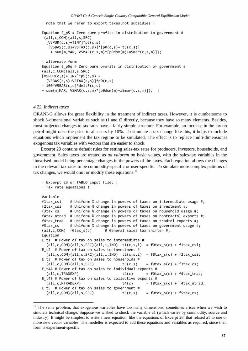
ORANI-G: A Generic Single-Country Computable General Equilibrium Model
37
! note that we refer to export taxes,not subsidies !
Equation E_p5 # Zero pure profits in distribution to government # (all,c,COM)(all,s,SRC) [V5PUR(c,s)+TINY]*p5(c,s) = [V5BAS(c,s)+V5TAX(c,s)]*[p0(c,s)+ t5(c,s)] + sum{m,MAR, V5MAR(c,s,m)*[p0dom(m)+a5mar(c,s,m)]};
! alternate formEquation E_p5q # Zero pure profits in distribution of government #(all,c,COM)(all,s,SRC)[V5PUR(c,s)+TINY]*p5(c,s) = [V5BAS(c,s)+V5TAX(c,s)]*p0(c,s)+ 100*V5BAS(c,s)*delt5(c,s)+ sum{m,MAR, V5MAR(c,s,m)*[p0dom(m)+a5mar(c,s,m)]}; !
4.22. Indirect taxes
ORANI-G allows for great flexibility in the treatment of indirect taxes. However, it is cumbersome toshock 3-dimensional variables such as t1 and t2 directly, because they have so many elements. Besides,most projected changes to tax rates have a fairly simple structure. For example, an increase in the tax onpetrol might raise the price to all users by 10%. To simulate a tax change like this, it helps to includeequations which implement the tax regime to be simulated. The effect is to replace multi-dimensionalexogenous tax variables with vectors that are easier to shock.
Excerpt 23 contains default rules for setting sales-tax rates for producers, investors, households, andgovernment. Sales taxes are treated as ad valorem on basic values, with the sales-tax variables in thelinearised model being percentage changes in the powers of the taxes. Each equation allows the changesin the relevant tax rates to be commodity-specific or user-specific. To simulate more complex patterns oftax changes, we would omit or modify these equations.16
! Excerpt 23 of TABLO input file: !! Tax rate equations !
Variablef1tax_csi # Uniform % change in powers of taxes on intermediate usage #;f2tax_csi # Uniform % change in powers of taxes on investment #;f3tax_cs # Uniform % change in powers of taxes on household usage #;f4tax_ntrad # Uniform % change in powers of taxes on nontradtnl exports #;f4tax_trad # Uniform % change in powers of taxes on tradtnl exports #;f5tax_cs # Uniform % change in powers of taxes on government usage #;(all,c,COM) f0tax_s(c) # General sales tax shifter #;EquationE_t1 # Power of tax on sales to intermediate # (all,c,COM)(all,s,SRC)(all,i,IND) t1(c,s,i) = f0tax_s(c) + f1tax_csi;E_t2 # Power of tax on sales to investment # (all,c,COM)(all,s,SRC)(all,i,IND) t2(c,s,i) = f0tax_s(c) + f2tax_csi;E_t3 # Power of tax on sales to households # (all,c,COM)(all,s,SRC) t3(c,s) = f0tax_s(c) + f3tax_cs;E_t4A # Power of tax on sales to individual exports # (all,c,TRADEXP) t4(c) = f0tax_s(c) + f4tax_trad;E_t4B # Power of tax on sales to collective exports # (all,c,NTRADEXP) t4(c) = f0tax_s(c) + f4tax_ntrad;E_t5 # Power of tax on sales to government # (all,c,COM)(all,s,SRC) t5(c,s) = f0tax_s(c) + f5tax_cs;
16 The same problem, that exogenous variables have too many dimensions, sometimes arises when we wish tosimulate technical change. Suppose we wished to shock the variable a1 (which varies by commodity, source andindustry). It might be simplest to write a new equation, like the equations of Excerpt 28, that related a1 to one ormore new vector variables. The modeller is expected to add these equations and variables as required, since theirform is experiment-specific.

Mark Horridge
38
The equations of Excerpt 24 compute ordinary changes in the indirect tax flows. Their main use is inthe Update statements for the various commodity tax matrices (see above). To understand the equations,note that the bases for the sales taxes are the basic values of the corresponding commodity flows, and thetax-rate variables appearing in the model are powers of the sales-tax rates. Hence, for any component ofsales tax, we can express revenue (VTAX), in levels, as the product of the base (VBAS) and the power ofthe tax (T) minus one, i.e.,
VTAX = VBAS(T-1). (31)
Hence: VTAX = VBAS(T-1) + VBAST,
= VBAS(T-1)VBASVBAS + VBAS*T
TT ,
= VBAS(T-1)wbas/100 + VBAS*T*t/100,
= VTAX*wbas/100 + (VBAS+VTAX)t/100,
where wbas and t are percentage changes in VBAS and T. VBAS is in turn a product of a quantity (X)and a basic price (P), so its percentage change wbas can be written as (x + p). Hence:
VTAX = VTAX(x+p)/100 + (VBAS+VTAX)t/100 (32)
The RHS shows two components of revenue change; due to changes in the base and rate respectively.
! Excerpt 24 of TABLO input file: !! Update formulae for commodity taxes !
Equation E_delV1TAX (all,c,COM)(all,s,SRC)(all,i,IND) delV1TAX(c,s,i) = 0.01*V1TAX(c,s,i)* [x1(c,s,i) + p0(c,s)] + 0.01*[V1BAS(c,s,i)+V1TAX(c,s,i)]*t1(c,s,i); E_delV2TAX (all,c,COM)(all,s,SRC)(all,i,IND) delV2TAX(c,s,i)= 0.01*V2TAX(c,s,i)* [x2(c,s,i) + p0(c,s)] + 0.01*[V2BAS(c,s,i)+V2TAX(c,s,i)]*t2(c,s,i); E_delV3TAX (all,c,COM)(all,s,SRC) delV3TAX(c,s) = 0.01*V3TAX(c,s)* [x3(c,s) + p0(c,s)] + 0.01*[V3BAS(c,s)+V3TAX(c,s)]*t3(c,s); E_delV4TAX (all,c,COM) delV4TAX(c) = 0.01*V4TAX(c)* [x4(c) + pe(c)] + 0.01*[V4BAS(c)+V4TAX(c)]*t4(c); E_delV5TAX (all,c,COM)(all,s,SRC) delV5TAX(c,s) = 0.01*V5TAX(c,s)*[x5(c,s) + p0(c,s)] + 0.01*[V5BAS(c,s)+V5TAX(c,s)]*t5(c,s);
! alternate formE_delV5TAX (all,c,COM)(all,s,SRC) delV5TAX(c,s) = 0.01*V5TAX(c,s)*[x5(c,s) + p0(c,s)] + V5BAS(c,s)*delt5(c,s); !
The comment at the end shows how the final equation would appear if the t5 variable (% change inpower) was replaced by delt5: an ordinary change in the ad valorem rate.

ORANI-G: A Generic Single-Country Computable General Equilibrium Model
39
In the next excerpt, equation E_p0B relates the domestic-currency prices of imports (c.i.f., duty-paid)to their foreign-currency prices. It is derived from the levels form:
P0(c,"imp") = PF0CIF(c)*PHI*T0IMP(c). (33)
The other equation computes changes in tariff revenues, used to update V0TAR.
! Excerpt 25 of TABLO input file: !! Import prices and tariff revenue !
Variable(all,c,COM) pf0cif(c) # C.I.F. foreign currency import prices #;(all,c,COM) t0imp(c) # Power of tariff #;
Equation E_p0B # Zero pure profits in importing #(all,c,COM) p0(c,"imp") = pf0cif(c) + phi + t0imp(c);
Equation E_delV0TAR (all,c,COM) delV0TAR(c) = 0.01*V0TAR(c)*[x0imp(c)+pf0cif(c)+phi] + 0.01*V0IMP(c)*t0imp(c);
Excerpt 26 computes various aggregates of indirect tax revenue—both in the levels and in ordinarychange form. Both equations and formulae are simple add-ups.
! Excerpt 26 of TABLO input file: !! Indirect tax revenue aggregates !Coefficient V1TAX_CSI # Total intermediate tax revenue #; V2TAX_CSI # Total investment tax revenue #; V3TAX_CS # Total households tax revenue #; V4TAX_C # Total export tax revenue #; V5TAX_CS # Total government tax revenue #; V0TAR_C # Total tariff revenue #;Formula V1TAX_CSI = sum{c,COM, sum{s,SRC, sum{i,IND, V1TAX(c,s,i)}}}; V2TAX_CSI = sum{c,COM, sum{s,SRC, sum{i,IND, V2TAX(c,s,i)}}}; V3TAX_CS = sum{c,COM, sum{s,SRC, V3TAX(c,s)}}; V4TAX_C = sum{c,COM, V4TAX(c)}; V5TAX_CS = sum{c,COM, sum{s,SRC, V5TAX(c,s)}}; V0TAR_C = sum{c,COM, V0TAR(c)};Variable(change) delV1tax_csi # Aggregate revenue from indirect taxes on intermediate #;(change) delV2tax_csi # Aggregate revenue from indirect taxes on investment #;(change) delV3tax_cs # Aggregate revenue from indirect taxes on households #;(change) delV4tax_c # Aggregate revenue from indirect taxes on export #;(change) delV5tax_cs # Aggregate revenue from indirect taxes on government #;(change) delV0tar_c # Aggregate tariff revenue #;
EquationE_delV1tax_csi delV1tax_csi = sum{c,COM,sum{s,SRC,sum{i,IND, delV1TAX(c,s,i)}}};E_delV2tax_csi delV2tax_csi = sum{c,COM,sum{s,SRC,sum{i,IND, delV2TAX(c,s,i)}}};E_delV3tax_cs delV3tax_cs = sum{c,COM,sum{s,SRC, delV3TAX(c,s)}};E_delV4tax_c delV4tax_c = sum{c,COM, delV4TAX(c)};E_delV5tax_cs delV5tax_cs = sum{c,COM,sum{s,SRC,delV5TAX(c,s)}};E_delV0tar_c delV0tar_c = sum{c,COM, delV0TAR(c)};

Mark Horridge
40
4.23. GDP from the income and expenditure sides
Excerpt 27 defines the nominal aggregates which make up GDP from the income side. These includetotals of factor payments, the value of other costs, and the total yield from commodity taxes. Their deri-vation is straightforward. For example, the formula for total land revenue:
V1LND_I = Sum{i,IND, V1LND(i)} = Sum{i,IND, X1LND(i)*P1LND(i) },
becomes, in percentage-change form:
V1LND_I*w1lnd_i = Sum{i,IND, V1LND(i)*[x1lnd(i)+p1lnd(i)]}.
! Excerpt 27 of TABLO input file: !! Factor incomes and GDP !
Coefficient V1CAP_I # Total payments to capital #; V1LAB_IO # Total payments to labour #; V1LND_I # Total payments to land #; V1PTX_I # Total production tax/subsidy #; V1OCT_I # Total other cost ticket payments #; V1PRIM_I # Total primary factor payments#; V0GDPINC # Nominal GDP from income side #; V0TAX_CSI # Total indirect tax revenue #;Formula V1CAP_I = sum{i,IND, V1CAP(i)}; V1LAB_IO = sum{i,IND, V1LAB_O(i)}; V1LND_I = sum{i,IND, V1LND(i)}; V1PTX_I = sum{i,IND, V1PTX(i)}; V1OCT_I = sum{i,IND, V1OCT(i)}; V1PRIM_I = V1LAB_IO + V1CAP_I + V1LND_I; V0TAX_CSI = V1TAX_CSI + V2TAX_CSI + V3TAX_CS + V4TAX_C + V5TAX_CS + V0TAR_C + V1OCT_I + V1PTX_I; V0GDPINC = V1PRIM_I + V0TAX_CSI;
Variable w1lab_io # Aggregate payments to labour #; w1cap_i # Aggregate payments to capital #; w1lnd_i # Aggregate payments to land #; w1prim_i # Aggregate primary factor payments #; w1oct_i # Aggregate "other cost" ticket payments #; (change) delV1PTX_i # Ordinary change in all‐industry production tax revenue #; (change) delV0tax_csi # Aggregate revenue from all indirect taxes #; w0tax_csi # Aggregate revenue from all indirect taxes #; w0gdpinc # Nominal GDP from income side #;Equation E_w1lab_io V1LAB_IO*w1lab_io = sum{i,IND,sum{o,OCC, V1LAB(i,o)*[x1lab(i,o)+p1lab(i,o)]}}; E_w1cap_i V1CAP_I*w1cap_i = sum{i,IND, V1CAP(i)*[x1cap(i)+p1cap(i)]}; E_w1lnd_i ID01[V1LND_I]*w1lnd_i = sum{i,IND, V1LND(i)*[x1lnd(i)+p1lnd(i)]}; E_w1prim_i V1PRIM_I*w1prim_i=V1LAB_IO*w1lab_io+V1CAP_I*w1cap_i+V1LND_I*w1lnd_i; E_w1oct_i ID01[V1OCT_I]*w1oct_i = sum{i,IND, V1OCT(i)*[x1oct(i)+p1oct(i)]}; E_delV1PTX_i delV1PTX_i = sum{i,IND,delV1PTX(i)}; E_delV0tax_csi delV0tax_csi = delV1tax_csi + delV2tax_csi + delV3tax_cs + delV4tax_c + delV5tax_cs + delV0tar_c + delV1PTX_i + 0.01*V1OCT_I*w1oct_i; E_w0tax_csi [TINY+V0TAX_CSI]*w0tax_csi = 100*delV0tax_csi; E_w0gdpinc V0GDPINC*w0gdpinc = V1PRIM_I*w1prim_i + 100*delV0tax_csi;
Because TABLO does not distinguish upper and lower case, we cannot use 'v1lnd_i' to refer to thechange in V1LND_I—instead we use 'w1lnd_i'. This conflict arises only for aggregate flows, since onlythese flows appear simultaneously as variables and coefficients.
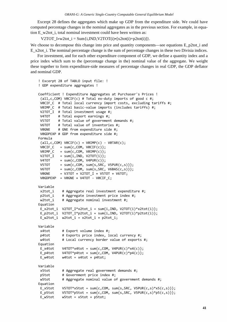
ORANI-G: A Generic Single-Country Computable General Equilibrium Model
41
Excerpt 28 defines the aggregates which make up GDP from the expenditure side. We could havecomputed percentage changes in the nominal aggregates as in the previous section. For example, in equa-tion E_w2tot_i, total nominal investment could have been written as:
V2TOT_I*w2tot_i = Sum{i,IND,V2TOT(i)*[x2tot(i)+p2tot(i)]}.
We choose to decompose this change into price and quantity components—see equations E_p2tot_i andE_x2tot_i. The nominal percentage change is the sum of percentage changes in these two Divisia indices.
For investment, and for each other expenditure component of GDP, we define a quantity index and aprice index which sum to the (percentage change in the) nominal value of the aggregate. We weightthese together to form expenditure-side measures of percentage changes in real GDP, the GDP deflatorand nominal GDP.
! Excerpt 28 of TABLO input file: !! GDP expenditure aggregates !
Coefficient ! Expenditure Aggregates at Purchaser's Prices ! (all,c,COM) V0CIF(c) # Total ex‐duty imports of good c #; V0CIF_C # Total local currency import costs, excluding tariffs #; V0IMP_C # Total basic‐value imports (includes tariffs) #; V2TOT_I # Total investment usage #; V4TOT # Total export earnings #; V5TOT # Total value of government demands #; V6TOT # Total value of inventories #; V0GNE # GNE from expenditure side #; V0GDPEXP # GDP from expenditure side #;Formula (all,c,COM) V0CIF(c) = V0IMP(c) ‐ V0TAR(c); V0CIF_C = sum{c,COM, V0CIF(c)}; V0IMP_C = sum{c,COM, V0IMP(c)}; V2TOT_I = sum{i,IND, V2TOT(i)}; V4TOT = sum{c,COM, V4PUR(c)}; V5TOT = sum{c,COM, sum{s,SRC, V5PUR(c,s)}}; V6TOT = sum{c,COM, sum{s,SRC, V6BAS(c,s)}}; V0GNE = V3TOT + V2TOT_I + V5TOT + V6TOT; V0GDPEXP = V0GNE + V4TOT ‐ V0CIF_C;
Variable x2tot_i # Aggregate real investment expenditure #; p2tot_i # Aggregate investment price index #; w2tot_i # Aggregate nominal investment #;Equation E_x2tot_i V2TOT_I*x2tot_i = sum{i,IND, V2TOT(i)*x2tot(i)}; E_p2tot_i V2TOT_I*p2tot_i = sum{i,IND, V2TOT(i)*p2tot(i)}; E_w2tot_i w2tot_i = x2tot_i + p2tot_i;
Variable x4tot # Export volume index #; p4tot # Exports price index, local currency #; w4tot # Local currency border value of exports #;Equation E_x4tot V4TOT*x4tot = sum{c,COM, V4PUR(c)*x4(c)}; E_p4tot V4TOT*p4tot = sum{c,COM, V4PUR(c)*p4(c)}; E_w4tot w4tot = x4tot + p4tot;
Variable x5tot # Aggregate real government demands #; p5tot # Government price index #; w5tot # Aggregate nominal value of government demands #;Equation E_x5tot V5TOT*x5tot = sum{c,COM, sum{s,SRC, V5PUR(c,s)*x5(c,s)}}; E_p5tot V5TOT*p5tot = sum{c,COM, sum{s,SRC, V5PUR(c,s)*p5(c,s)}}; E_w5tot w5tot = x5tot + p5tot;

Mark Horridge
42
Variable x6tot # Aggregate real inventories #; p6tot # Inventories price index #; w6tot # Aggregate nominal value of inventories #;Equation E_x6tot [TINY+V6TOT]*x6tot =100*sum{c,COM,sum{s,SRC,LEVP0(c,s)*delx6(c,s)}}; E_p6tot [TINY+V6TOT]*p6tot = sum{c,COM, sum{s,SRC, V6BAS(c,s)*p0(c,s)}}; E_w6tot w6tot = x6tot + p6tot;
Variable x0cif_c # Import volume index, C.I.F. weights #; p0cif_c # Imports price index, C.I.F., local currency #; w0cif_c # C.I.F. local currency value of imports #;Equation E_x0cif_c V0CIF_C*x0cif_c = sum{c,COM, V0CIF(c)*x0imp(c)}; E_p0cif_c V0CIF_C*p0cif_c = sum{c,COM, V0CIF(c)*[phi+pf0cif(c)]}; E_w0cif_c w0cif_c = x0cif_c + p0cif_c;
Variable !section added Oct 2002! x0gne # Real GNE from expenditure side #; p0gne # GNE price index, expenditure side #; w0gne # Nominal GNE from expenditure side #;Equation E_x0gne V0GNE*x0gne = V3TOT*x3tot + V2TOT_I*x2tot_i + V5TOT*x5tot +V6TOT*x6tot; E_p0gne V0GNE*p0gne = V3TOT*p3tot + V2TOT_I*p2tot_i + V5TOT*p5tot +V6TOT*p6tot; E_w0gne w0gne = x0gne + p0gne;
Variable x0gdpexp # Real GDP from expenditure side #; p0gdpexp # GDP price index, expenditure side #; w0gdpexp # Nominal GDP from expenditure side #;Equation E_x0gdpexp x0gdpexp = [1/V0GDPEXP]*[V3TOT*x3tot + V2TOT_I*x2tot_i + V5TOT*x5tot + V6TOT*x6tot + V4TOT*x4tot ‐ V0CIF_C*x0cif_c]; E_p0gdpexp p0gdpexp = [1/V0GDPEXP]*[V3TOT*p3tot + V2TOT_I*p2tot_i + V5TOT*p5tot + V6TOT*p6tot + V4TOT*p4tot ‐ V0CIF_C*p0cif_c]; E_w0gdpexp w0gdpexp = x0gdpexp + p0gdpexp;
Superficially, price and quantity components such as p2tot_i and x2tot_i resemble the price andquantity indices which arise from the nested production functions of agents. The latter Divisia indicesarise from homothetic functional forms. However, the model contains no analogous function to aggre-gate investment quantities across industries. Similarly, our definition of real consumption is not derivedfrom the household utility function. We use these price-quantity decompositions only as convenientsummary measures17.
It is an accounting identity that GDP from the expenditure and income sides must be equal, both inthe levels and in percentage changes. That is:
V0GDPEXP V0GDPINC, and w0gdpexp w0gdpinc. (34)Nonetheless, we find it useful to compute and print these values separately as a check on the model's ac-counting relations.
17 There is indeed no levels equation corresponding to our change definition of, say, the investment price index. Alevels formulation could use either initial or final weights; our formula uses weights that vary continuouslybetween these two values. Because our formula for p2tot_i can only be written in change form, results for thatvariable suffer from path-dependence: they depend slightly on details of the solution algorithm that should beirrelevant. The effect however is normally very small, and rarely propagates through to other equations.

ORANI-G: A Generic Single-Country Computable General Equilibrium Model
43
4.24. The trade balance and other aggregates
Because zero is a plausible base-period value, the balance of trade is computed in the first equation inExcerpt 29 as an ordinary change (delB), not a percentage change. We avoid choosing units by express-ing this change as a fraction of GDP. Note that delB is the [change in the] ratio of two nominal variables.
The next three equations measure percentage changes in imports at tariff-inclusive prices. Finally,the excerpt contains measures of percentage changes in the terms of trade and the real exchange rate.
! Excerpt 29 of TABLO input file: !! Trade balance and other indices !
Variable (change) delB # (Nominal balance of trade)/{nominal GDP} #; x0imp_c # Import volume index, duty‐paid weights #; w0imp_c # Value of imports plus duty #; p0imp_c # Duty‐paid imports price index, local currency #; p0realdev # Real devaluation #; p0toft # Terms of trade #;Equation E_delB 100*V0GDPEXP*delB=V4TOT*w4tot ‐V0CIF_C*w0cif_c‐[V4TOT‐V0CIF_C]*w0gdpexp; E_x0imp_c x0imp_c = sum{c,COM, [V0IMP(c)/V0IMP_C]*x0imp(c)}; E_p0imp_c p0imp_c = sum{c,COM, [V0IMP(c)/V0IMP_C]*p0(c,"imp")}; E_w0imp_c w0imp_c = x0imp_c + p0imp_c; E_p0toft p0toft = p4tot ‐ p0cif_c; E_p0realdev p0realdev = p0cif_c ‐ p0gdpexp;
4.25. Primary factor aggregates
Excerpt 30 begins by computing some quantity measures of employment, capital usage, and GDP atfactor cost. These aggregates indicate the aggregate productive capacities of the relevant factors. Forexample, in computing the aggregate employment measures, we use wage-bill weights, reflecting therelative marginal products of different workers. Different aggregates could be defined, using as weightshours worked, or numbers employed18.
Next are computed three indices of primary factor prices.
! Excerpt 30 of TABLO input file: !! Primary factor aggregates !
Variable (all,i,IND) employ(i) # Employment by industry #; employ_i # Aggregate employment: wage bill weights #; x1cap_i # Aggregate capital stock, rental weights #; x1lnd_i # Aggregate land stock, rental weights #; x1prim_i # Aggregate effective primary factor use #; xgdpfac # Real GDP at factor cost (inputs) = x1prim_i #; p1prim_i # Index of factor cost #; p1lab_io # Average nominal wage #; realwage # Average real wage #; p1cap_i # Average capital rental #; p1lnd_i # Average land rental #;Equation E_employ (all,i,IND) V1LAB_O(i)*employ(i) = sum{o,OCC, V1LAB(i,o)*x1lab(i,o)}; E_employ_i V1LAB_IO*employ_i = sum{i,IND, V1LAB_O(i)*employ(i)}; E_x1cap_i V1CAP_I*x1cap_i = sum{i,IND, V1CAP(i)*x1cap(i)}; E_x1lnd_i ID01[V1LND_I]*x1lnd_i = sum{i,IND, V1LND(i)*x1lnd(i)}; E_x1prim_i V1PRIM_I*x1prim_i = sum{i,IND, V1PRIM(i)*x1prim(i)}; E_xgdpfac xgdpfac = [1/V1PRIM_I]* [V1LAB_IO*employ_i + V1CAP_I*x1cap_i + V1LND_I*x1lnd_i];
18 The TABLO input file contains optional code, not shown here, which could be used to compute such indices,data permitting.

Mark Horridge
44
E_p1prim_i V1PRIM_I*p1prim_i = sum{i,IND, V1PRIM(i)*p1prim(i)}; E_p1lab_io V1LAB_IO*p1lab_io = sum{i,IND, sum{o,OCC, V1LAB(i,o)*p1lab(i,o)}}; E_realwage realwage = p1lab_io ‐ p3tot; E_p1cap_i V1CAP_I*p1cap_i = sum{i,IND, V1CAP(i)*p1cap(i)}; E_p1lnd_i ID01[V1LND_I]*p1lnd_i = sum{i,IND, V1LND(i)*p1lnd(i)};
4.26. Rates of return and investment
Excerpt 31 contains equations determining x2tot, the amount of new capital stock created for each in-dustry. In recent years, ORANI has evolved into a dynamic model and the specification of investmentbehaviour has been in a state of flux. ORANI-G contains 3 alternate investment rules, one of which willbe active for each industry. The active rule either determines industry investment, or (if aggregateinvestment is fixed) it determines that industry's share in aggregate investment.
Rule 1 relates the creation of new capital stock in each industry to profitability in that industry. Itfollows the original ORANI computer model. For a fuller explanation, the reader is referred to DPSV,Section 19. The effect of the equation is that industries which become more profitable (gret(i) rising)attract more investment (higher ggro(i)).
Equation E_finv1 relates the investment/capital ratio to the rate of return (relative to the variableinvslack, which is interpretable here as an economy-wide rate of return). It is to be interpreted as a risk-related relationship with relatively fast- (slow-) growing industries requiring premia (acceptingdiscounts) on their rates of return. If exogenous, the variable finv1(i) could be shocked to allow for ad-ditional shifts in investment. If, for some industry, finv1(i) is endogenous (and x2tot(i) is determined insome other way), equation E_finv1 serves only to determine finv1(i), which appears in no otherequation.
Rule 2, given by Equation E_finv2, may be used to determine investment in those industries forwhich Rule 1 is deemed inappropriate. These might be industries where investment is determined bygovernment policy. For such an industry the corresponding element of finv2 should be exogenous,causing that industry's investment to follow the national trend. For the other industries, E_finv2 just de-termines finv2.
Rule 3, given by Equation E_finv3, is intended for long run simulations. For an industry with fixedfinv3, it fixes gross capital growth rates (ggro=I/K ratios). The effect is that investment follows theindustry capital stock.
If the variable invslack is exogenous, the preceding equations will determine investment by industry,and therefore in aggregate. However, many short-run simulations have aggregate investment exogenous.This is made possible by leaving the variable invslack endogenous, with x2tot_i exogenous. Or, usingequation E_f2tot, link aggregate investment to aggregate real consumption by holding f2tot exogenouswith invslack endogenous.
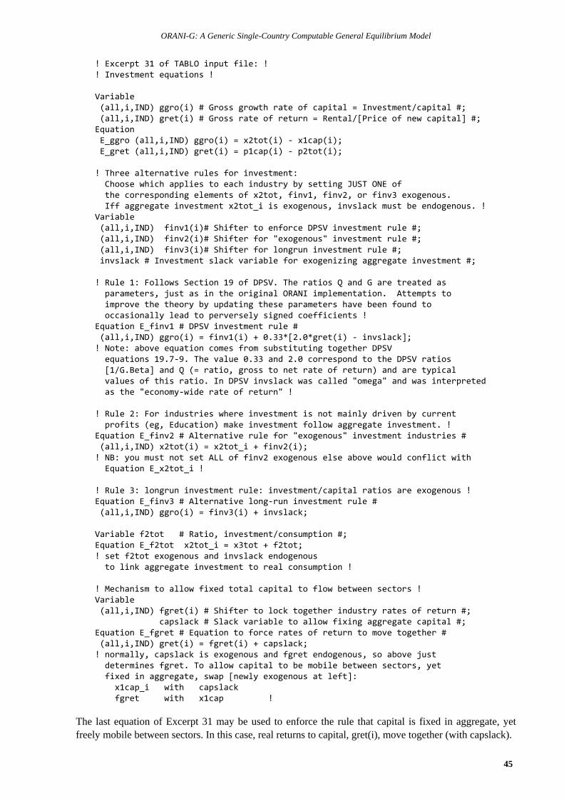
ORANI-G: A Generic Single-Country Computable General Equilibrium Model
45
! Excerpt 31 of TABLO input file: !! Investment equations !
Variable (all,i,IND) ggro(i) # Gross growth rate of capital = Investment/capital #; (all,i,IND) gret(i) # Gross rate of return = Rental/[Price of new capital] #;Equation E_ggro (all,i,IND) ggro(i) = x2tot(i) ‐ x1cap(i); E_gret (all,i,IND) gret(i) = p1cap(i) ‐ p2tot(i);
! Three alternative rules for investment: Choose which applies to each industry by setting JUST ONE of the corresponding elements of x2tot, finv1, finv2, or finv3 exogenous. Iff aggregate investment x2tot_i is exogenous, invslack must be endogenous. !Variable (all,i,IND) finv1(i)# Shifter to enforce DPSV investment rule #; (all,i,IND) finv2(i)# Shifter for "exogenous" investment rule #; (all,i,IND) finv3(i)# Shifter for longrun investment rule #; invslack # Investment slack variable for exogenizing aggregate investment #;
! Rule 1: Follows Section 19 of DPSV. The ratios Q and G are treated as parameters, just as in the original ORANI implementation. Attempts to improve the theory by updating these parameters have been found to occasionally lead to perversely signed coefficients !Equation E_finv1 # DPSV investment rule # (all,i,IND) ggro(i) = finv1(i) + 0.33*[2.0*gret(i) ‐ invslack];! Note: above equation comes from substituting together DPSV equations 19.7‐9. The value 0.33 and 2.0 correspond to the DPSV ratios [1/G.Beta] and Q (= ratio, gross to net rate of return) and are typical values of this ratio. In DPSV invslack was called "omega" and was interpreted as the "economy‐wide rate of return" !
! Rule 2: For industries where investment is not mainly driven by current profits (eg, Education) make investment follow aggregate investment. !Equation E_finv2 # Alternative rule for "exogenous" investment industries # (all,i,IND) x2tot(i) = x2tot_i + finv2(i);! NB: you must not set ALL of finv2 exogenous else above would conflict with Equation E_x2tot_i !
! Rule 3: longrun investment rule: investment/capital ratios are exogenous !Equation E_finv3 # Alternative long‐run investment rule # (all,i,IND) ggro(i) = finv3(i) + invslack;
Variable f2tot # Ratio, investment/consumption #;Equation E_f2tot x2tot_i = x3tot + f2tot;! set f2tot exogenous and invslack endogenous to link aggregate investment to real consumption !
! Mechanism to allow fixed total capital to flow between sectors !Variable (all,i,IND) fgret(i) # Shifter to lock together industry rates of return #; capslack # Slack variable to allow fixing aggregate capital #;Equation E_fgret # Equation to force rates of return to move together # (all,i,IND) gret(i) = fgret(i) + capslack;! normally, capslack is exogenous and fgret endogenous, so above just determines fgret. To allow capital to be mobile between sectors, yet fixed in aggregate, swap [newly exogenous at left]: x1cap_i with capslack fgret with x1cap !
The last equation of Excerpt 31 may be used to enforce the rule that capital is fixed in aggregate, yetfreely mobile between sectors. In this case, real returns to capital, gret(i), move together (with capslack).

Mark Horridge
46
4.27. The labour market
Like ORANI, ORANI-G contains no theory of labour supply. Users of the model have the option of set-ting employment exogenously, with market-clearing wage rates determined endogenously, or settingwage rates (real or nominal) exogenously, allowing employment to be demand determined.
In Excerpt 32, equation E_x1lab_i computes changes in the aggregate demand for labour of eachskill. Equation E_p1lab is a wage setting equation. In the standard ORANI short-run closure, the 'f1lab'variables are exogenous, so that all wages are indexed to the CPI. Then, if shocked, the 'f1lab' variablesallow for deviations in the growth of some or all wages relative to the growth of the CPI. This short-runlabour market closure was originally devised to reflect the centralised wage-fixing mechanisms that usedto operate in Australia. However, it has proven popular in quite different contexts. It assumes that labouris mobile between industries, and that supply of each skill type is elastic.
As a variant on the standard shortrun closure, the average nominal wage, p1lab_io, may be fixed,while endogenizing the overall wage shifter, f1lab_io. The effect will be to fix all the p1lab, giving themodel a Keynesian flavour.
The typical long-run closure sets employ_i (aggregate employment: wage bill weights) exogenous,while endogenizing the overall wage shifter, f1lab_io. The other 'f1lab' variables remain exogenous, re-flecting fixed wage relativities. This assumes that labour is mobile between industries and occupations.
These labour-market modelling decisions are usually made at an economy-wide level, but could beapplied individually and perhaps differentially to different industries or types of labour. For example, wecould exogenize the supply of skilled workers and the wages of unskilled workers. Or, we couldexogenize employment in agriculture and wages in other sectors19.
In the standard long-run and short-run closures, wage relativities are fixed, so firms do not substitutebetween labour of different types. Thus the values of SIGMA1LAB, the CES substitution elasticity be-tween skill types, do not affect simulation results. This is handy for the modeller who is agnostic aboutthose values (econometric evidence is scant). The more exotic labour market closures, which do allowwage relativities to change, focus attention on the values assumed for SIGMA1LAB.
! Excerpt 32 of TABLO input file: !! Labour market !
Variable (all,i,IND)(all,o,OCC) f1lab(i,o) # Wage shift variable #; (all,o,OCC) f1lab_i(o) # Occupation‐specific wage shifter #; (all,o,OCC) x1lab_i(o) # Employment by occupation #; (all,i,IND) f1lab_o(i) # Industry‐specific wage shifter #; f1lab_io # Overall wage shifter #;
Coefficient (all,o,OCC) V1LAB_I(o) # Total wages, occupation o #;Formula (all,o,OCC) V1LAB_I(o) = sum{i,IND, V1LAB(i,o)};Equation E_x1lab_i # Demand equals supply for labour of each skill # (all,o,OCC) V1LAB_I(o)*x1lab_i(o) = sum{i,IND, V1LAB(i,o)*x1lab(i,o)};
E_p1lab # Flexible setting of money wages # (all,i,IND)(all,o,OCC) p1lab(i,o)= p3tot + f1lab_io + f1lab_o(i) + f1lab_i(o) + f1lab(i,o);
Variable (all,o,OCC) p1lab_i(o) # Average wage of occupation #;Equation E_p1lab_i # Average wage of occupation # (all,o,OCC) V1LAB_I(o)*p1lab_i(o) = sum{i,IND, V1LAB(i,o)*p1lab(i,o)};
4.28. Miscellaneous equations
Equation E_p1oct in Excerpt 33 allows for indexation of the unit price of 'other costs' to the CPI. Thevariable f1oct(i) can be interpreted as the percentage change in the real price of 'other costs' to industry i. 19 The TABLO input file contains optional code, not shown here, to implement upward-sloping labour supplyschedules.

ORANI-G: A Generic Single-Country Computable General Equilibrium Model
47
Equation E_f3tot implements a simple, optional, consumption function. If f3tot is exogenous, theequation links household spending to nominal GDP. Otherwise, there is no effect on the rest of the sys-tem, since the variable f3tot appears nowhere else.
The next two equations define two vector variables, p0dom and p0imp, which are simply equal to thecorresponding columns of the basic price matrix, p0. They are included to facilitate the viewing ofsimulation results: in that situation, vectors are often more convenient to work with than are matrices.
The equations described thus far define the main part of ORANI-G. The remaining excerpts of theTABLO input file contain supplementary material which does not directly affect simulation results.
! Excerpt 33 of TABLO input file: !! Miscellaneous equations !
Variable (all,i,IND) f1oct(i)# Shift in price of "other cost" tickets #;Equation E_p1oct # Indexing of prices of "other cost" tickets # (all,i,IND) p1oct(i) = p3tot + f1oct(i); ! assumes full indexation !
Variable f3tot # Ratio, consumption/ GDP #;Equation E_f3tot # Consumption function # w3tot = w0gdpexp + f3tot;
! Map between vector and matrix forms of basic price variables !Variable (all,c,COM) p0imp(c) # Basic price of imported goods = p0(c,"imp") #;Equation E_p0dom # Basic price of domestic goods = p0(c,"dom") # (all,c,COM) p0dom(c) = p0(c,"dom");Equation E_p0imp # Basic price of imported goods = p0(c,"imp") # (all,c,COM) p0imp(c) = p0(c,"imp");
4.29. Adding variables for explaining results
Part of the ORANI tradition is that simulation results, although voluminous, must all be capable of ver-bal explanation based on model equations and data. It is customary to examine and present results ingreat detail. The aim is to dispel any tendency to treat the model as a black box. These detailed analysessometimes yield theoretical insights; for example, we may find that some mechanism which we thoughtto be of minor significance exerts a dominant force in certain sectors. More often we discover errors—either in the data or in the model equations. Inappropriate theory may also lead to implausible results.
Results analysis, then, is an indispensable (but laborious) part of quality control for an economicmodel. To make it less painful, we often add equations and variables merely to help explain results. Thenext two excerpts are examples of this type of addition.
4.30. Sales decomposition
The sales decomposition, implemented in Excerpt 34, breaks down the percentage change in the totalsales of each commodity into various intermediate and final demand categories. This would be useful,for example, if we wondered whether an increase in motor vehicle output was due to increases in eitherinvestment or household demand.
To decompose a percentage change in this way (i.e., find parts which add up to the whole), we haveto perform some arithmetical manipulations. Suppose we have a variable X which is the sum of 2 parts:
X = A + B or PX = PA + PB (where P is a common price) (35)
then, for small percentage changes, we can write:
x = conta+ contb where conta = (PA/PX)a and contb = (PB/PX)b (36)
We call conta and contb the contributions of A and B to the percentage change in X.For larger changes, which require a multistep computation, equation (36) would result in values for contaand contb which did not quite add up to the total percentage change in X20. To avoid this, it is useful tospecify both conta and contb as ordinary change variables and to define a new ordinary change variable,
20 The reason is that during a multistep computation percentage changes are compounded, whilst ordinary changesare added.
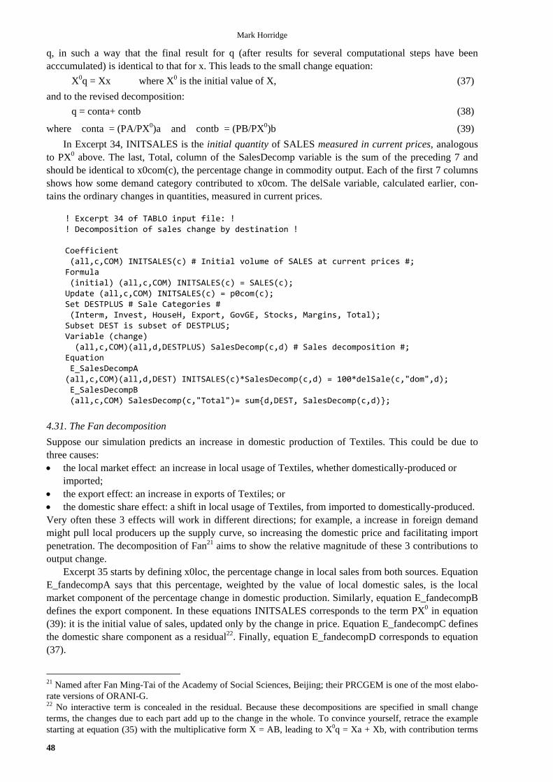
Mark Horridge
48
q, in such a way that the final result for q (after results for several computational steps have beenacccumulated) is identical to that for x. This leads to the small change equation:
X0q = Xx where X0 is the initial value of X, (37)
and to the revised decomposition:
q = conta+ contb (38)
where conta = (PA/PX0)a and contb = (PB/PX0)b (39)
In Excerpt 34, INITSALES is the initial quantity of SALES measured in current prices, analogousto PX0 above. The last, Total, column of the SalesDecomp variable is the sum of the preceding 7 andshould be identical to x0com(c), the percentage change in commodity output. Each of the first 7 columnsshows how some demand category contributed to x0com. The delSale variable, calculated earlier, con-tains the ordinary changes in quantities, measured in current prices.
! Excerpt 34 of TABLO input file: !! Decomposition of sales change by destination !
Coefficient (all,c,COM) INITSALES(c) # Initial volume of SALES at current prices #;Formula (initial) (all,c,COM) INITSALES(c) = SALES(c);Update (all,c,COM) INITSALES(c) = p0com(c);Set DESTPLUS # Sale Categories # (Interm, Invest, HouseH, Export, GovGE, Stocks, Margins, Total);Subset DEST is subset of DESTPLUS;Variable (change) (all,c,COM)(all,d,DESTPLUS) SalesDecomp(c,d) # Sales decomposition #;Equation E_SalesDecompA(all,c,COM)(all,d,DEST) INITSALES(c)*SalesDecomp(c,d) = 100*delSale(c,"dom",d); E_SalesDecompB (all,c,COM) SalesDecomp(c,"Total")= sum{d,DEST, SalesDecomp(c,d)};
4.31. The Fan decomposition
Suppose our simulation predicts an increase in domestic production of Textiles. This could be due tothree causes: the local market effectan increase in local usage of Textiles, whether domestically-produced or
imported; the export effect: an increase in exports of Textiles; or the domestic share effect: a shift in local usage of Textiles, from imported to domestically-produced.Very often these 3 effects will work in different directions; for example, a increase in foreign demandmight pull local producers up the supply curve, so increasing the domestic price and facilitating importpenetration. The decomposition of Fan21 aims to show the relative magnitude of these 3 contributions tooutput change.
Excerpt 35 starts by defining x0loc, the percentage change in local sales from both sources. EquationE_fandecompA says that this percentage, weighted by the value of local domestic sales, is the localmarket component of the percentage change in domestic production. Similarly, equation E_fandecompBdefines the export component. In these equations INITSALES corresponds to the term PX0 in equation(39): it is the initial value of sales, updated only by the change in price. Equation E_fandecompC definesthe domestic share component as a residual22. Finally, equation E_fandecompD corresponds to equation(37).
21 Named after Fan Ming-Tai of the Academy of Social Sciences, Beijing; their PRCGEM is one of the most elabo-rate versions of ORANI-G.22 No interactive term is concealed in the residual. Because these decompositions are specified in small changeterms, the changes due to each part add up to the change in the whole. To convince yourself, retrace the examplestarting at equation (35) with the multiplicative form X = AB, leading to X0q = Xa + Xb, with contribution terms

ORANI-G: A Generic Single-Country Computable General Equilibrium Model
49
! Excerpt 35 of TABLO input file: !! Decomposition of Fan !
Set FANCAT # Parts of Fan decomposition # (LocalMarket, DomShare, Export, Total);Variable(all,c,COM) x0loc(c) # Real percent change in LOCSALES (dom+imp) #;(change)(all,c,COM)(all,f,FANCAT) fandecomp(c,f) # Fan decomposition #;Coefficient (all,c,COM) LOCSALES(c) # Total local sales of dom + imp good c #;Formula (all,c,COM) LOCSALES(c) = DOMSALES(c) + V0IMP(c);
Equation E_x0loc # %Growth in local market # (all,c,COM) LOCSALES(c)*x0loc(c) = DOMSALES(c)*x0dom(c) + V0IMP(c)*x0imp(c);
E_fandecompA # Growth in local market effect # (all,c,COM) INITSALES(c)*fandecomp(c,"LocalMarket") = DOMSALES(c)*x0loc(c);! The local market effect is the % change in output that would have occurredif local sales of the domestic product had followed dom+imp sales (x0loc) !
E_fandecompB # Export effect # (all,c,COM) INITSALES(c)*fandecomp(c,"Export") = V4BAS(c)*x4(c);
E_fandecompC # Import leakage effect ‐ via residual # (all,c,COM) fandecomp(c,"Total") = fandecomp(c,"LocalMarket") + fandecomp(c,"DomShare") + fandecomp(c,"Export");
E_fandecompD # Fan total = x0com # (all,c,COM) INITSALES(c)*fandecomp(c,"Total") = SALES(c)*x0com(c);
4.32. The expenditure side GDP decomposition
Excerpt 36 breaks down changes in real GDP into the contributions of the main expenditure-sideaggregates (contGDPexp). This enables us to quickly see how much of the change in real expenditure-side GDP is due, say, to a change in aggregate investment. The mathematics is the same as that of theSales decomposition in Excerpt 34. For convenience, the contributions of exports and imports are com-bined into the variable contBOT. Note that contBOT, like each component of contGDPexp, is a realcontribution: it takes no account of changes in export or import prices. It is the same (apart from units ofmeasurement) as the B variable in the original ORANI model.
(X/X0)a and (X/X0)b. However, the cumulative results of these contributions can be defined only as a path integralof the contribution terms computed at each solution step. Hence they are not (quite) invariant to the details of oursolution procedure. See also footnote 17.
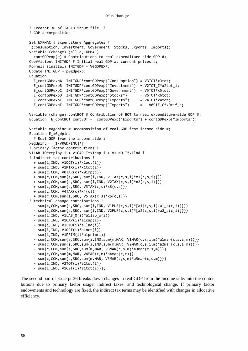
Mark Horridge
50
! Excerpt 36 of TABLO input file: !! GDP decomposition !
Set EXPMAC # Expenditure Aggregates # (Consumption, Investment, Government, Stocks, Exports, Imports);Variable (change) (all,e,EXPMAC) contGDPexp(e) # Contributions to real expenditure‐side GDP #;Coefficient INITGDP # Initial real GDP at current prices #;Formula (initial) INITGDP = V0GDPEXP;Update INITGDP = p0gdpexp;Equation E_contGDPexpA INITGDP*contGDPexp("Consumption") = V3TOT*x3tot; E_contGDPexpB INITGDP*contGDPexp("Investment") = V2TOT_I*x2tot_i; E_contGDPexpC INITGDP*contGDPexp("Government") = V5TOT*x5tot; E_contGDPexpD INITGDP*contGDPexp("Stocks") = V6TOT*x6tot; E_contGDPexpE INITGDP*contGDPexp("Exports") = V4TOT*x4tot; E_contGDPexpF INITGDP*contGDPexp("Imports") = ‐ V0CIF_C*x0cif_c;
Variable (change) contBOT # Contribution of BOT to real expenditure‐side GDP #;Equation E_contBOT contBOT = contGDPexp("Exports") + contGDPexp("Imports");
Variable x0gdpinc # Decomposition of real GDP from income side #;Equation E_x0gdpinc # Real GDP from the income side #x0gdpinc = [1/V0GDPINC]*[! primary factor contributions !V1LAB_IO*employ_i + V1CAP_I*x1cap_i + V1LND_I*x1lnd_i! indirect tax contributions ! + sum{i,IND, V1OCT(i)*x1oct(i)} + sum{i,IND, V1PTX(i)*x1tot(i)} + sum{c,COM, V0TAR(c)*x0imp(c)} + sum{c,COM,sum{s,SRC, sum{i,IND, V1TAX(c,s,i)*x1(c,s,i)}}} + sum{c,COM,sum{s,SRC, sum{i,IND, V2TAX(c,s,i)*x2(c,s,i)}}} + sum{c,COM,sum{s,SRC, V3TAX(c,s)*x3(c,s)}} + sum{c,COM, V4TAX(c)*x4(c)} + sum{c,COM,sum{s,SRC, V5TAX(c,s)*x5(c,s)}}! technical change contributions ! ‐ sum{c,COM,sum{s,SRC, sum{i,IND, V1PUR(c,s,i)*[a1(c,s,i)+a1_s(c,i)]}}} ‐ sum{c,COM,sum{s,SRC, sum{i,IND, V2PUR(c,s,i)*[a2(c,s,i)+a2_s(c,i)]}}} ‐ sum{i,IND, V1LAB_O(i)*a1lab_o(i)} ‐ sum{i,IND, V1CAP(i)*a1cap(i)} ‐ sum{i,IND, V1LND(i)*a1lnd(i)} ‐ sum{i,IND, V1OCT(i)*a1oct(i)} ‐ sum{i,IND, V1PRIM(i)*a1prim(i)} ‐ sum{c,COM,sum{s,SRC,sum{i,IND,sum{m,MAR, V1MAR(c,s,i,m)*a1mar(c,s,i,m)}}}} ‐ sum{c,COM,sum{s,SRC,sum{i,IND,sum{m,MAR, V2MAR(c,s,i,m)*a2mar(c,s,i,m)}}}} ‐ sum{c,COM,sum{s,SRC,sum{m,MAR, V3MAR(c,s,m)*a3mar(c,s,m)}}} ‐ sum{c,COM,sum{m,MAR, V4MAR(c,m)*a4mar(c,m)}} ‐ sum{c,COM,sum{s,SRC,sum{m,MAR, V5MAR(c,s,m)*a5mar(c,s,m)}}} ‐ sum{i,IND, V2TOT(i)*a2tot(i)} ‐ sum{i,IND, V1CST(i)*a1tot(i)}];
The second part of Excerpt 36 breaks down changes in real GDP from the income side: into the contri-butions due to primary factor usage, indirect taxes, and technological change. If primary factorendowments and technology are fixed, the indirect tax terms may be identified with changes in allocativeefficiency.

ORANI-G: A Generic Single-Country Computable General Equilibrium Model
51
4.33. Checking the data
A model rendered in the TABLO language is a type of computer program, and like other computer pro-grams tends to contain errors. We employ a number of strategies to prevent errors and to make errorsapparent. One strategy is to check all conditions which the initial data must satisfy. This is done in Ex-cerpt 37. The conditions are: The row sums of the MAKE matrix must equal the row sums of the BAS and MAR rows of Figure 4.
That is, the output of domestically produced commodities must equal the total of the demands forthem.
The column sums of the MAKE matrix must equal the sum of the first, producers', column of Figure4. That is, the value of output by each industry must equal the total of production costs.
The average value of the household expenditure elasticities, EPS, should be one. The average shouldbe computed using the expenditure weights, V3PUR_S.To check these conditions, the items PURE_PROFITS, LOST_GOODS, and EPSTOT are stored on
the SUMMARY file. Their values should be near to zero (or one, for EPSTOT).The Assertion statements which come next enforce the above rules. If the specified condition is not
met during some simulation, GEMPACK will stop with an error message indicating which condition isnot satisfied. The first two Assertions are checked before every stage of a multi-step simulation. The lastone, for EPSTOT, should be true before and after (but not necessarily during) a simulation.
It should be emphasized that the validity of percentage change equations depends on the validity ofthe data from which the equation coefficients are calculated. The GEMPACK solution method must startfrom a database which is consistent, in the levels, with all the equations.
There are other formal tests which can reveal errors in model formulation. These are set out in Ap-pendix I.
! Excerpt 37 of TABLO input file: !! Check identities !
Coefficient ! coefficients for checking ! (all,i,IND) DIFFIND(i) # COSTS‐MAKE_C : should be zero #; (all,c,COM) DIFFCOM(c) # SALES‐MAKE_I : should be zero #; EPSTOT # Average Engel elasticity: should = 1 #;Formula (all,i,IND) DIFFIND(i) = V1TOT(i) ‐ MAKE_C(i); (all,c,COM) DIFFCOM(c) = SALES(c) ‐ MAKE_I(c); EPSTOT = sum{c,COM, S3_S(c)*EPS(c)};
Write ! we file these numbers BEFORE the assertions below ! DIFFIND to file SUMMARY header "DIND"; DIFFCOM to file SUMMARY header "DCOM"; EPSTOT to file SUMMARY header "ETOT";
Assertion ! if below not true, program will stop with message ! # DIFFIND = V1TOT‐MAKE_C = tiny # (all,i,IND) ABS[DIFFIND(i)/V1TOT(i)] <0.001; # DIFFCOM = SALES‐MAKE_I = tiny # (all,c,COM) ABS[DIFFCOM(c)/SALES(c)] <0.001; (initial) # Average Engel elasticity = 1 # ABS[1‐EPSTOT] <0.001;
4.34. Summarizing the data
The next few Excerpts collect together various summaries of the data and store these on file in a formthat is convenient for later viewing. These summaries are useful for checking the plausibility of data andfor explaining simulation results. Excerpt 38 groups into vectors the various components of, first, GDPfrom the expenditure side; second, GDP from the income side; and third, the components of total indirecttaxes23.
23 GEMPACK stores data in its own, binary, format. A Windows program, ViewHAR, is normally used forviewing or modifying these so-called HAR files. The data matrices created here are designed to be convenient for

Mark Horridge
52
! Excerpt 38 of TABLO input file: !! Summary: components of GDP from income and expenditure sides !
Coefficient (all,e,EXPMAC) EXPGDP(e) # Expenditure Aggregates #;Formula EXPGDP("Consumption") = V3TOT; EXPGDP("Investment") = V2TOT_I; EXPGDP("Government") = V5TOT; EXPGDP("Stocks") = V6TOT; EXPGDP("Exports") = V4TOT; EXPGDP("Imports") = ‐V0CIF_C;Write EXPGDP to file SUMMARY header "EMAC";
Set INCMAC # Income Aggregates # (Land, Labour, Capital, IndirectTax);Coefficient (all,i,INCMAC) INCGDP(i) # Income Aggregates #;Formula INCGDP("Land") = V1LND_I; INCGDP("Labour") = V1LAB_IO; INCGDP("Capital") = V1CAP_I; INCGDP("IndirectTax") = V0TAX_CSI;Write INCGDP to file SUMMARY header "IMAC";
Set TAXMAC # Tax Aggregates # (Intermediate,Investment,Consumption,Exports,Government,OCT,ProdTax,Tariff);Coefficient (all,t,TAXMAC) TAX(t) # Tax Aggregates #;Formula TAX("Intermediate") = V1TAX_CSI; TAX("Investment") = V2TAX_CSI; TAX("Consumption") = V3TAX_CS; TAX("Exports") = V4TAX_C; TAX("Government") = V5TAX_CS; TAX("OCT") = V1OCT_I; TAX("ProdTax") = V1PTX_I; TAX("Tariff") = V0TAR_C;Write TAX to file SUMMARY header "TMAC";
Excerpt 39 forms a matrix showing the main parts of production cost for each industry.
! Excerpt 39 of TABLO input file: !! Summary: matrix of industry costs !
Set COSTCAT # Cost Categories # (IntDom, IntImp, Margin, ComTax, Lab, Cap, Lnd, ProdTax, OCT);Coefficient (all,i,IND)(all,co,COSTCAT) COSTMAT(i,co) # Cost Matrix #;Formula (all,i,IND) COSTMAT(i,"IntDom") = sum{c,COM, V1BAS(c,"dom",i)}; (all,i,IND) COSTMAT(i,"IntImp") = sum{c,COM, V1BAS(c,"imp",i)}; (all,i,IND) COSTMAT(i,"Margin") = sum{c,COM, sum{s,SRC, sum{m,MAR, V1MAR(c,s,i,m)}}}; (all,i,IND) COSTMAT(i,"ComTax") = sum{c,COM, sum{s,SRC, V1TAX(c,s,i)}}; (all,i,IND) COSTMAT(i,"Lab") = V1LAB_O(i); (all,i,IND) COSTMAT(i,"Cap") = V1CAP(i); (all,i,IND) COSTMAT(i,"Lnd") = V1LND(i); (all,i,IND) COSTMAT(i,"ProdTax") = V1PTX(i); (all,i,IND) COSTMAT(i,"OCT") = V1OCT(i);Write COSTMAT to file SUMMARY header "CSTM";
examining with ViewHAR. ViewHAR automatically calculates and displays subtotals, so that total GDP, forexample, does not need to be included in the summary vectors defined here.

ORANI-G: A Generic Single-Country Computable General Equilibrium Model
53
Excerpt 40 calculates for each main destination, the basic, margin, and commodity tax components ofpurchases by commodity and source.
! Excerpt 40 of TABLO input file: !! Summary: basic, margins and taxes !SetSALECAT2 # SALE Categories # (Interm, Invest, HouseH, Export, GovGE, Stocks);FLOWTYPE # Type of flow # (Basic, Margin, TAX);Coefficient(all,c,COM)(all,f,FLOWTYPE)(all,s,SRC)(all,sa,SALECAT2) SALEMAT2(c,f,s,sa) # Basic, margin and tax components of purchasers' values #;Formula(all,c,COM)(all,f,FLOWTYPE)(all,s,SRC)(all,sa,SALECAT2) SALEMAT2(c,f,s,sa)=0;(all,c,COM)(all,s,SRC) SALEMAT2(c,"Basic",s,"Interm") = sum{i,IND,V1BAS(c,s,i)};(all,c,COM)(all,s,SRC) SALEMAT2(c,"Tax" ,s,"Interm") = sum{i,IND,V1TAX(c,s,i)};(all,c,COM)(all,s,SRC) SALEMAT2(c,"Margin",s,"Interm") = sum{i,IND, sum{m,MAR, V1MAR(c,s,i,m)}};(all,c,COM)(all,s,SRC) SALEMAT2(c,"Basic",s,"Invest") = sum{i,IND,V2BAS(c,s,i)};(all,c,COM)(all,s,SRC) SALEMAT2(c,"Tax" ,s,"Invest") = sum{i,IND,V2TAX(c,s,i)};(all,c,COM)(all,s,SRC) SALEMAT2(c,"Margin",s,"Invest") = sum{i,IND, sum{m,MAR, V2MAR(c,s,i,m)}};(all,c,COM)(all,s,SRC) SALEMAT2(c,"Basic",s,"HouseH") = V3BAS(c,s);(all,c,COM)(all,s,SRC) SALEMAT2(c,"Tax" ,s,"HouseH") = V3TAX(c,s);(all,c,COM)(all,s,SRC) SALEMAT2(c,"Margin",s,"HouseH")= sum{m,MAR,V3MAR(c,s,m)};(all,c,COM)(all,s,SRC) SALEMAT2(c,"Basic",s,"GovGE") = V5BAS(c,s);(all,c,COM)(all,s,SRC) SALEMAT2(c,"Tax" ,s,"GovGE") = V5TAX(c,s);(all,c,COM)(all,s,SRC) SALEMAT2(c,"Margin",s,"GovGE")= sum{m,MAR,V5MAR(c,s,m)};(all,c,COM) SALEMAT2(c,"Basic","dom","Export") = V4BAS(c);(all,c,COM) SALEMAT2(c,"Tax" ,"dom","Export") = V4TAX(c);(all,c,COM) SALEMAT2(c,"Margin","dom","Export")= sum{m,MAR,V4MAR(c,m)};(all,c,COM)(all,s,SRC) SALEMAT2(c,"Basic",s,"Stocks") = V6BAS(c,s);Write SALEMAT2 to file SUMMARY header "MKUP";
4.35. Import shares and short-run supply elasticities
Excerpt 41 computes and stores 2 more items which help explain results. The higher is the import shareIMPSHR for some commodity, the more vulnerable is the associated local industry to importcompetition.
Short-run simulation results are often coloured by the effects of inelastic supply schedules for capi-tal-intensive industries. We compute and store the short-run supply elasticity SUPPLYELAST to helpidentify such industries. The formula used is derived in Appendix J. The closely-related primary factorshares can be seen from the FACTOR matrix (using the row shares feature of the GEMPACK programViewHAR).
! Excerpt 41 of TABLO input file: !! Import shares and short‐run supply elasticities !
Coefficient (all,c,COM) IMPSHR(c) # Share of imports in local market #;Formula (all,c,COM) IMPSHR(c) = V0IMP(c)/[TINY+DOMSALES(c)+V0IMP(c)];Write IMPSHR to file SUMMARY header "MSHR";
Coefficient (all,i,IND) SUPPLYELAST(i) # Short‐run supply elasticity #;Zerodivide default 999;Zerodivide (nonzero_by_zero) default 999;Formula (all,i,IND) SUPPLYELAST(i) = SIGMA1PRIM(i)*V1LAB_O(i)*V1TOT(i)/[V1PRIM(i)*{V1CAP(i)+V1LND(i)}];Zerodivide off;Zerodivide (nonzero_by_zero) off;Write SUPPLYELAST to file SUMMARY header "SRSE";
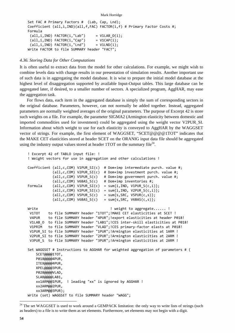
Mark Horridge
54
Set FAC # Primary Factors # (Lab, Cap, Lnd);Coefficient (all,i,IND)(all,f,FAC) FACTOR(i,f) # Primary Factor Costs #;Formula (all,i,IND) FACTOR(i,"Lab") = V1LAB_O(i); (all,i,IND) FACTOR(i,"Cap") = V1CAP(i); (all,i,IND) FACTOR(i,"Lnd") = V1LND(i);Write FACTOR to file SUMMARY header "FACT";
4.36. Storing Data for Other Computations
It is often useful to extract data from the model for other calculations. For example, we might wish tocombine levels data with change results in our presentation of simulation results. Another important useof such data is in aggregating the model database. It is wise to prepare the initial model database at thehighest level of disaggregation supported by available Input-Output tables. This large database can beaggregated later, if desired, to a smaller number of sectors. A specialized program, AggHAR, may easethe aggregation task.
For flows data, each item in the aggregated database is simply the sum of corresponding sectors inthe original database. Parameters, however, can not normally be added together. Instead, aggregatedparameters are normally weighted averages of the original parameters. The purpose of Excerpt 42 is storesuch weights on a file. For example, the parameter SIGMA2 (Armington elasticity between domestic andimported commodities used for investment) could be aggregated using the weight vector V2PUR_SI.Information about which weight to use for each elasticity is conveyed to AggHAR by the WAGGSETvector of strings. For example, the first element of WAGGSET, “SCET@@@@1TOT” indicates thatthe MAKE CET elasticities stored at header SCET on the ORANIG input data file should be aggregatedusing the industry output values stored at header 1TOT on the summary file24.
! Excerpt 42 of TABLO input file: !! Weight vectors for use in aggregation and other calculations !
Coefficient (all,c,COM) V1PUR_SI(c) # Dom+imp intermediate purch. value #; (all,c,COM) V2PUR_SI(c) # Dom+imp investment purch. value #; (all,c,COM) V5PUR_S(c) # Dom+imp government purch. value #; (all,c,COM) V6BAS_S(c) # Dom+imp inventories #;Formula (all,c,COM) V1PUR_SI(c) = sum{i,IND, V1PUR_S(c,i)}; (all,c,COM) V2PUR_SI(c) = sum{i,IND, V2PUR_S(c,i)}; (all,c,COM) V5PUR_S(c) = sum{s,SRC, V5PUR(c,s)}; (all,c,COM) V6BAS_S(c) = sum{s,SRC, V6BAS(c,s)};
Write ! weight to aggregate...... ! V1TOT to file SUMMARY header "1TOT";!MAKE CET elasticities at SCET ! V4PUR to file SUMMARY header "4PUR";!export elasticities at header P018! V1LAB_O to file SUMMARY header "LAB1";!CES inter‐skill elasticities at P018! V1PRIM to file SUMMARY header "VLAD";!CES primary‐factor elasts at P018! V1PUR_SI to file SUMMARY header "1PUR";!Armington elasticities at 1ARM ! V2PUR_SI to file SUMMARY header "2PUR";!Armington elasticities at 2ARM ! V3PUR_S to file SUMMARY header "3PUR";!Armington elasticities at 2ARM !
Set WAGGSET # Instructions to AGGHAR for weighted aggregation of parameters # ( SCET@@@@1TOT, P018@@@@4PUR, ITEX@@@@4PUR, XPEL@@@@3PUR, P028@@@@VLAD, SLAB@@@@LAB1, xx1ARM@@1PUR, ! leading "xx" is ignored by AGGHAR ! xx2ARM@@2PUR, xx3ARM@@3PUR);Write (set) WAGGSET to file SUMMARY header "WAGG";
24 The set WAGGSET is used to work around a GEMPACK limitation: the only way to write lists of strings (suchas headers) to a file is to write them as set elements. Furthermore, set elements may not begin with a digit.
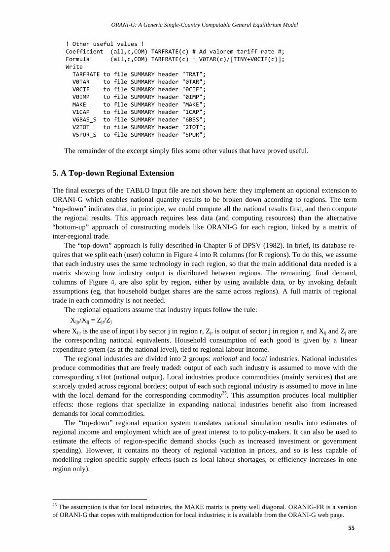
ORANI-G: A Generic Single-Country Computable General Equilibrium Model
55
! Other useful values !Coefficient (all,c,COM) TARFRATE(c) # Ad valorem tariff rate #;Formula (all,c,COM) TARFRATE(c) = V0TAR(c)/[TINY+V0CIF(c)];Write TARFRATE to file SUMMARY header "TRAT"; V0TAR to file SUMMARY header "0TAR"; V0CIF to file SUMMARY header "0CIF"; V0IMP to file SUMMARY header "0IMP"; MAKE to file SUMMARY header "MAKE"; V1CAP to file SUMMARY header "1CAP"; V6BAS_S to file SUMMARY header "6BSS"; V2TOT to file SUMMARY header "2TOT"; V5PUR_S to file SUMMARY header "5PUR";
The remainder of the excerpt simply files some other values that have proved useful.
5. A Top-down Regional Extension
The final excerpts of the TABLO Input file are not shown here: they implement an optional extension toORANI-G which enables national quantity results to be broken down according to regions. The term“top-down” indicates that, in principle, we could compute all the national results first, and then computethe regional results. This approach requires less data (and computing resources) than the alternative“bottom-up” approach of constructing models like ORANI-G for each region, linked by a matrix ofinter-regional trade.
The “top-down” approach is fully described in Chapter 6 of DPSV (1982). In brief, its database re-quires that we split each (user) column in Figure 4 into R columns (for R regions). To do this, we assumethat each industry uses the same technology in each region, so that the main additional data needed is amatrix showing how industry output is distributed between regions. The remaining, final demand,columns of Figure 4, are also split by region, either by using available data, or by invoking defaultassumptions (eg, that household budget shares are the same across regions). A full matrix of regionaltrade in each commodity is not needed.
The regional equations assume that industry inputs follow the rule:
Xijr/Xij = Zjr/Zj
where Xijr is the use of input i by sector j in region r, Zjr is output of sector j in region r, and Xij and Zj arethe corresponding national equivalents. Household consumption of each good is given by a linearexpenditure sytem (as at the national level), tied to regional labour income.
The regional industries are divided into 2 groups: national and local industries. National industriesproduce commodities that are freely traded: output of each such industry is assumed to move with thecorresponding x1tot (national output). Local industries produce commodities (mainly services) that arescarcely traded across regional borders; output of each such regional industry is assumed to move in linewith the local demand for the corresponding commodity25. This assumption produces local multipliereffects: those regions that specialize in expanding national industries benefit also from increaseddemands for local commodities.
The “top-down” regional equation system translates national simulation results into estimates ofregional income and employment which are of great interest to to policy-makers. It can also be used toestimate the effects of region-specific demand shocks (such as increased investment or governmentspending). However, it contains no theory of regional variation in prices, and so is less capable ofmodelling region-specific supply effects (such as local labour shortages, or efficiency increases in oneregion only).
25 The assumption is that for local industries, the MAKE matrix is pretty well diagonal. ORANIG-FR is a versionof ORANI-G that copes with multiproduction for local industries; it is available from the ORANI-G web page.

Mark Horridge
56
6. Closing the Model
The model specified in Section 4 has more variables than equations. To close the model, we choosewhich variables are to be exogenous and which endogenous26. The number of endogenous variables mustequal the number of equations. For a complex AGE model, it may be surprisingly difficult to find a sen-sible closure which satisfies this accounting restriction.
Table 2 allows us to attack the task systematically. It arranges the model's 132 equations and 179variables according to their dimensions. Equations broken into parts, such as E_x4A (covering individualexport commodities) and E_x4B (covering collective exports) are treated as one equation block for thispurpose. The first column lists the various combinations of set indices that occur in the model. Thesecond column shows how many variables have these combinations. For example, 10 variables aredimensioned by COM, SRC and IND. The third column counts equations in the same way. For example,there are 56 macro, i.e., scalar, equations.
In most straightforward closures of the model, the correspondence between equations and endoge-nous variables applies for each row of the table, as well as in total. The fourth column shows thedifference between the preceding two, i.e, it shows how many variables of that size would normally beexogenous.
Table 2 Tally of Variables and Equations
1
Dimension
2
Variable
Count
3
Equation
Count
4
Exogenous
Count
5
List of unexplained variables
(Mechanical closure)
MACRO 71 56 15
f1lab_io f4p_ntrad phi f4q_ntrad q f4tax_trad
f4tax_ntrad f5tot2 capslack invslack w3lux
f1tax_csi f2tax_csi f3tax_cs f5tax_cs
COM 25 19 6 f0tax_s t0imp a3_s f4p f4q pf0cif
COM*IND 7 5 2 a1_s a2_s
COM*MAR 2 1 1 a4mar
COM*SRC 14 11 3 f5 a3 fx6
COM*SRC*IND 10 8 2 a1 a2
COM*SRC*IND*MAR 4 2 2 a1mar a2mar
COM*SRC*MAR 4 2 2 a3mar a5mar
IND 34 21 13 a1cap a1lab_o a1lnd a1oct a1prim a1tot
f1lab_o f1oct x2tot x1lnd a2tot x1cap
delPTXRate
IND*OCC 3 2 1 f1lab
OCC 2 1 1 f1lab_I
COM*SRC*DEST 1 1 0
COM*DESTPLUS 1 1 0
COM*FANCAT 1 1 0
EXPMAC 1 1 0
TOTAL 179 132 47
In constructing the TABLO Input file, we chose to name each equation after the variable it seemed toexplain or determine27. Some variables had no equation named after them—they appear in the fifthcolumn. Those variables are promising candidates for exogeneity. They include:
26 In GEMPACK parlance, a closure is a list of exogenous variables.27 If equations are named after variables, the GEMPACK program TABmate will automatically perform theanalysis summarized in Table 2. The equation naming system is slightly arbitrary. For example, where a supplyequation and a demand equation jointly determine price and quantity, we could say that the supply equation ex-plained the price variable, and that the demand equation explained the quantity variable. Or we could pair supplywith quantity and demand with price. It would not matter which way we chose: the two equations between themendogenize both price and quantity.

ORANI-G: A Generic Single-Country Computable General Equilibrium Model
57
technical change variables, mostly beginning with the letter 'a'; tax rate variables, mostly beginning with 't'; shift variables, mostly beginning with 'f'; land endowments x1lnd, and the number of households q; industry capital stocks, x1cap; foreign prices, pf0cif, and the investment slack variable, invslack; inventory to sales ratios, fx6; the exchange rate phi, which could serve as numeraire; and w3lux (household above-subsistence expenditure).
Although Column 5 contains a perfectly valid exogenous set for the model, we choose, for typicalshortrun simulations, to adopt a slightly different closure. The macro variables italicised in Column 5 areswapped as follows. We exogenize x5tot instead of f5tot2, so disconnecting government from household consumption. We exogenize x2tot_i (aggregate investment), rather than invslack. We exogenize x3tot (household consumption), rather than w3lux. We exogenize delx6 (inventory changes), rather than fx6. We exogenize realwage (average real wage), rather than f1lab_io (overall wage shift). For each industry, we exogenize the corresponding element of either finv1 or finv2 in place of the
x2tot vector.These changes give rise to the closure shown in Table 3 (swapped variables are italicized).
Table 3 The ORANI short-run closure
Exogenous variables constraining real GDP from the supply sidex1cap x1lnd industry-specific endowments of capital and landcapslack allows industry-specific rates of returna1cap a1lab_o a1lnd a1prim a1tot a2tot all technological changerealwage average real wage
Exogenous settings of real GDP from the expenditure sidex3tot aggregate real private consumption expenditurex2tot_i aggregate real investment expenditurex5tot aggregate real government expendituref5 distribution of government demandsdelx6 real demands for inventories by commodity
Foreign conditions: import prices fixed; export demand curves fixed in quantity and price axespf0cif foreign prices of importsf4p f4q individual exportsf4p_ntrad f4q_ntrad collective exports
All tax rates are exogenousdelPTXRATE f0tax_s f1tax_csi f2tax_csi f3tax_csf5tax_cs t0imp f4tax_trad f4tax_ntrad f1oct
Distribution of investment between industriesfinv1(selected industries) investment related to profitsfinv2(the rest) investment follows aggregate investment
Number of households and their consumption preferences are exogenousq number of householdsa3_s household tastes
Numeraire assumptionphi nominal exchange rate
A choice of closure reflects two different types of consideration. First, the closure is associated with ouridea of the simulation timescale, that is, the period of time which would be needed for economic vari-
To name some other equations, we must have a closure in mind. For example, the factor demand equations of
Excerpt 8 are named E_x1lab_o, E_p1cap, and E_p1lnd. Thus the equation names suggest that the labour demandequation determines employment while the other two equations determine the unit rentals of capital and land. Thatnaming choice reflects the standard ORANI short-run closure, which fixes industry use of capital and land.

Mark Horridge
58
ables to adjust to a new equilibrium. The timescale assumption affects the way we model factor markets.For example, in a shortrun simulation we normally hold capital stocks fixed, as in Table 3. The idea isthat capital stocks take some time to install—too long for them to be affected, in the short run, by theshocks. Shortrun closures often also allow for rigidities in the labour market: in this case by holding realwages fixed. The length of the 'short' run is not explicit, but is usually thought to be between 1 and 3years.
Second, the choice of closure is affected by the needs of a particular simulation and by our view ofthe most appropriate assumption for those variables that the model does not explain. For example,ORANI-G provides little theory to explain the size and composition of absorption. In Table 3 the majorexpenditure-side aggregates are simply held fixed. Therefore, if some shock reduced GDP, the balance oftrade (which is endogenous) might move towards deficit, reflecting national dis-saving. We might wishto prevent this by fixing the balance of trade, delB, instead of, say, x3tot. This would allow us to use theendogenous x3tot as a simple index of welfare.
Table 4 A possible long-run closure
Exogenous variables constraining real GDP from the supply sidegret gross sectoral rates of returncapslack allows industry-specific rates of returnx1lnd industry-specific endowments of landa1cap a1lab_o a1lnd a1prim a1tot a2tot all technological changeemploy_i total employment - wage weights
Exogenous settings of real GDP from the expenditure sidedelB balance of trade/GDPinvslack aggregate investment determined by industry specific
rulesf5tot2 link government demands to total householdf5 distribution of government demandsdelx6 real demands for inventories by commodity
Foreign conditions: import prices fixed; export demand curves fixed in quantity and price axespf0cif foreign prices of importsf4p f4q individual exportsf4p_ntrad f4q_ntrad collective exports
All tax rates are exogenousdelPTXRATE f0tax_s f1tax_csi f2tax_csi f3tax_cs f5f5tax_cs t0imp f4tax_trad f4tax_ntrad f1oct
Distribution of investment between industriesfinv3(selected industries) fixed investment/capital ratiosfinv2(the rest) investment follows aggregate investment
Number of households and their consumption preferences are exogenousq number of householdsa3_s household tastes
Numeraire assumptionphi nominal exchange rate
Table 4 shows a possible longrun closure. Differences from the shortrun closure of Table 3 areshown in italics. The main differences are: Capital stocks are free to adjust in such a way that fixed rates of return (gret) are maintained. An
open capital market is implicitly assumed, since there is no link between capital formation and do-mestic saving.
Aggregate employment is fixed and the real wage adjusts. This would be consistent with the ideathat both the labour force and the rate of unemployment (NAIRU) are, in the long run, determined bymechanisms outside of the model.
Household and government expenditure move together, to accomodate a balance of trade constraint:DelB (the balance of trade as a fraction of GDP) is fixed. The idea here is that, in the long run therest of the world might be reluctant to fund an increased trade deficit. Aggregate investment followsthe aggregate capital stock.

ORANI-G: A Generic Single-Country Computable General Equilibrium Model
59
Another possible closure, often used for small theoretical models in textbooks of international trade, isthe trade-theoretic closure. This is almost the same as the long-run closure just described except thataggregate capital x1cap_i is fixed instead of the variable capslack. Rates of return then move in unison toaccomodate the x1cap_i constraint. In this closure, capital and labour are both fixed in aggregate butmobile between industries.
It should be emphasized that, particularly in a more complex model, many closures might be used fordifferent purposes. There is not a unique natural or correct closure. On the other hand, every sensibleclosure must satisfy certain requirements. For example, price variables in the model's equations alwaysappear as price ratios; it is a feature of most neo-classical models that only relative prices matter. Thus, ifwe have a solution of the model, we can always create another solution just by increasing all local pricesby, say, 10%. Therefore, for the overall price level to be determined, there has to be at least oneexogenous variable measured in local currency units. This variable—there is normally just one—iscalled the numeraire. In Tables 3 and 4 the exchange rate, phi, is the numeraire. Another popular choiceis p3tot, the CPI.
For similar reasons, there is no mechanism in ORANI-G which would determine the total size of theeconomy. Some quantity variables must be exogenous: these often include primary factor endowmentsand final demand aggregates.
In summary, ORANI-G lacks theories which explain: Changes in the absolute price level. We have to exogenously set either the exchange rate or some
domestic price index. This setting determines, in an arbitrary way, whether changes in the real ex-change rate are manifested either as changes in domestic prices or as changes in the exchange rate.However, results for real variables are unaffected by this decision.
Labour supply. We have to exogenously set either the average wage level (real or nominal) or em-ployment. This setting determines whether a more buoyant labour market is manifested either ashigher wages or as greater employment.
Changes in the size and composition of absorption. Either we must set these exogenously or else thetrade balance must be fixed while one or more components of absorption adjust. This setting deter-mines whether increased national income appears either as increased absorption, or alternatively asan improved balance of trade.
As well as suggesting a closure, Table 2 allows us to estimate the size of our model. With its 23 com-modities, 22 industries, 2 sources, 2 margin goods and 2 occupations, the standard Australian version ofORANI-G has about 25,000 scalar variable elements and 17,000 scalar equations. A typical larger ver-sion of ORANI used for policy analysis might have 115 commodities, 113 industries, 2 sources, 9margin goods and 8 occupations, leading to 1.3 million variables and 0.75 million equations. In its rawform, such a model would be far too big to solve. The next section explains how GEMPACK can con-dense a model to manageable size.
7. Using GEMPACK to Solve the Model
Figures 12 and 13 show, in simplified form, the main stages in the GEMPACK process. The first andlargest task, the specification of the model's equations using the TABLO language, has been described atlength in the previous sections. This material is contained in the ORANIG.TAB file (at top left of thefigure).
The model as described so far has too many equations and variables for efficient solution. Theirnumbers are reduced by instructing the TABLO program to: omit specified variables from the system. This option is useful for variables which will be exogenous
and unshocked (zero percentage change). Normally it allows us to dispense with the bulk of the tech-nical change terms. Of course, the particular selection of omitted variables will alter in accordancewith the model simulations to be undertaken.
substitute out specified variables using specified equations. This results in fewer but more complexequations. Typically we use this method to eliminate multi-dimensional matrix variables which aredefined by simple equations. For example, the equation:

Mark Horridge
60
Equation E_x1_s # Demands for Commodity Composites #(All,c,COM)(All,i,IND) x1_s(c,i) ‐ {a1_s(c,i) + a1tot(i)} = x1tot(i);
which appears in Excerpt 10 of the TABLO Input file, can be used to substitute out variable x1_s. Infact the names of the ORANI-G equations are chosen to suggest which variable each equation couldeliminate.28
The variables for omission and the equation-variable pairs for substitution are listed in a second, instruc-tion, file: ORANIG.STI.
The TABLO program converts the TAB and STI files into a FORTRAN source file, ORANIG.FOR,which contains the model-specific code needed for a solution program.
The Fortran compiler combines ORANIG.FOR with other, general-purpose, code to produce the ex-ecutable program ORANIG.EXE, which can be used to solve the model specified by the user in the TABand STI files.
ORANIG.AXT ORANIG.AXS
ORANIG.FOR
ORANIG.TAB
ORANIG.EXE
Legend
Text File
Program
Binary File
FORTRANcompiler
ORANIG.STITABLO
program
Figure 12. Building a model-specific EXE file
Simulations are conducted using ORANIG.EXE. Its inputs are: a data file, containing input-output data and behavioural parameters. This data file contains all neces-
sary information about the initial equilibrium. user input from a text (CMF) file, which specifies:
(a) which variables are to be exogenous;(b) shocks to some exogenous variables;(c) into how many steps the computation is divided; and(d) the names of input and output files, and other details of the solution process.
Each simulation produces an SL4 (Solution) file. The SL4 file has a binary format: it may be viewedwith the non-model-specific Windows program ViewSOL.
28 Substituted variables are necessarily endogenous and are not stored in the results file. GEMPACK also allowsback-substituted variables; these do appear in the results file but use slightly more computing resources. GEMPACK only allows a variable to be substituted using a single equation of just the same dimensions. For alarger model, it is very important that the model equations and variables are arranged in a way that allows largematrix variables to be substituted or back-substituted.
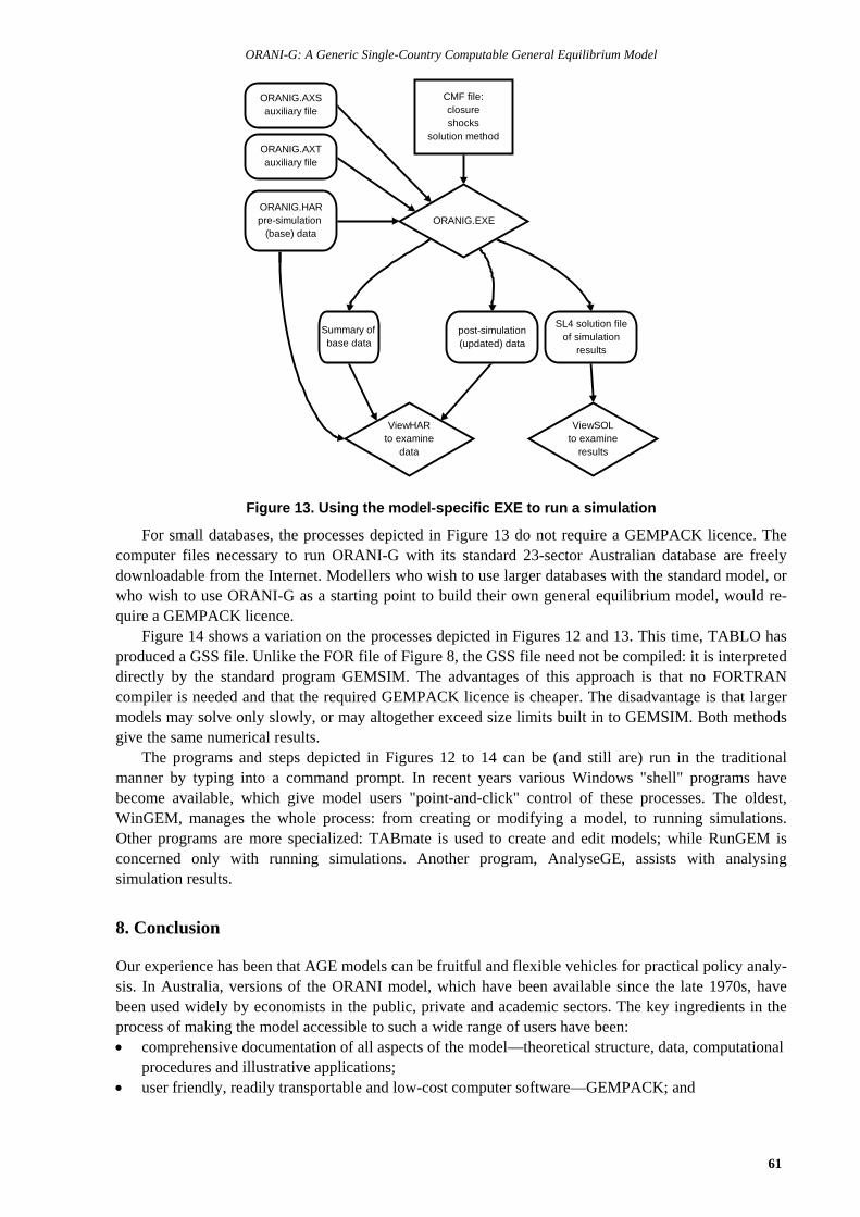
ORANI-G: A Generic Single-Country Computable General Equilibrium Model
61
ORANIG.AXTauxiliary file
ORANIG.AXSauxiliary file
ORANIG.EXE
CMF file:closureshocks
solution method
ORANIG.HARpre-simulation
(base) data
SL4 solution file of simulation
results
Summary of base data
post-simulation(updated) data
ViewHARto examine
data
ViewSOLto examine
results
Figure 13. Using the model-specific EXE to run a simulation
For small databases, the processes depicted in Figure 13 do not require a GEMPACK licence. Thecomputer files necessary to run ORANI-G with its standard 23-sector Australian database are freelydownloadable from the Internet. Modellers who wish to use larger databases with the standard model, orwho wish to use ORANI-G as a starting point to build their own general equilibrium model, would re-quire a GEMPACK licence.
Figure 14 shows a variation on the processes depicted in Figures 12 and 13. This time, TABLO hasproduced a GSS file. Unlike the FOR file of Figure 8, the GSS file need not be compiled: it is interpreteddirectly by the standard program GEMSIM. The advantages of this approach is that no FORTRANcompiler is needed and that the required GEMPACK licence is cheaper. The disadvantage is that largermodels may solve only slowly, or may altogether exceed size limits built in to GEMSIM. Both methodsgive the same numerical results.
The programs and steps depicted in Figures 12 to 14 can be (and still are) run in the traditionalmanner by typing into a command prompt. In recent years various Windows "shell" programs havebecome available, which give model users "point-and-click" control of these processes. The oldest,WinGEM, manages the whole process: from creating or modifying a model, to running simulations.Other programs are more specialized: TABmate is used to create and edit models; while RunGEM isconcerned only with running simulations. Another program, AnalyseGE, assists with analysingsimulation results.
8. Conclusion
Our experience has been that AGE models can be fruitful and flexible vehicles for practical policy analy-sis. In Australia, versions of the ORANI model, which have been available since the late 1970s, havebeen used widely by economists in the public, private and academic sectors. The key ingredients in theprocess of making the model accessible to such a wide range of users have been: comprehensive documentation of all aspects of the model—theoretical structure, data, computational
procedures and illustrative applications; user friendly, readily transportable and low-cost computer software—GEMPACK; and
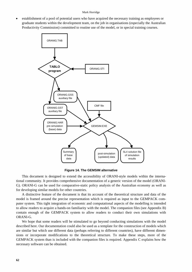
Mark Horridge
62
establishment of a pool of potential users who have acquired the necessary training as employees orgraduate students within the development team, on the job in organisations (especially the AustralianProductivity Commission) committed to routine use of the model, or in special training courses.
ORANIG.GSTauxiliary file
ORANIG.GSSauxiliary file
GEMSIM.EXE
CMF file
ORANIG.HARpre-simulation
(base) data
SL4 solution file of simulation
results
Summary of base
data
post-simulation(updated) data
ORANIG.TAB
ORANIG.STITABLO
program
Figure 14. The GEMSIM alternative
This document is designed to extend the accessibility of ORANI-style models within the interna-tional community. It provides comprehensive documentation of a generic version of the model (ORANI-G). ORANI-G can be used for comparative-static policy analysis of the Australian economy as well asfor developing similar models for other countries.
A distinctive feature of the document is that its account of the theoretical structure and data of themodel is framed around the precise representation which is required as input to the GEMPACK com-puter system. This tight integration of economic and computational aspects of the modelling is intendedto allow readers to acquire a hands-on familiarity with the model. The companion files (see Appendix B)contain enough of the GEMPACK system to allow readers to conduct their own simulations withORANI-G.
We hope that some readers will be stimulated to go beyond conducting simulations with the modeldescribed here. Our documentation could also be used as a template for the construction of models whichare similar but which use different data (perhaps referring to different countries), have different dimen-sions or incorporate modifications to the theoretical structure. To make these steps, more of theGEMPACK system than is included with the companion files is required. Appendix C explains how thenecessary software can be obtained.

ORANI-G: A Generic Single-Country Computable General Equilibrium Model
63
References
Black Book - see Dixon, Parmenter, Powell & Wilcoxen (1992).
Green Book (DPSV) - see Dixon, Parmenter,Sutton & Vincent (1982).
Yellow Book - see Dixon, Bowles & Kendrick (1980).
Orange Book - see Dixon, Powell & Parmenter (1979).
Armington PS (1969) The Geographic Pattern of Trade and the Effects of Price Changes, IMF Staff Papers,XVI, July, pp 176-199.
Armington PS (1970) Adjustment of Trade Balances: Some Experiments with a Model of Trade AmongMany Countries, IMF Staff Papers, XVII, November, pp 488-523.
Cooper R, McLaren K and Powell A (1985) Macroeconomic Closure in Applied General EquilibriumModelling: Experience from ORANI and Agenda for Further Research, in J. Piggot and J. Whalley (eds),New Developments in Applied General Equilibrium Analysis, New York: Cambridge University Press.
Dixon PB, Bowles S and Kendrick D (1980) Notes and Problems in Microeconomic Theory, Amsterdam:North-Holland.
Dixon PB, Parmenter BR, Powell AA and Wilcoxen PJ (1992) Notes and Problems in Applied GeneralEquilibrium Economics, Amsterdam: North-Holland.
Dixon PB, Parmenter BR, Ryland GJ and Sutton JM (1977) ORANI, A General Equilibrium Model of theAustralian Economy: Current Specification and Illustrations of Use for Policy Analysis—First ProgressReport of the IMPACT Project, Vol 2, Canberra:Australian Government Publishing Service.
Dixon PB, Powell A and Parmenter BR (1979) Structural Adaptation in an Ailing Macro-economy,Melbourne University Press.
Dixon PB, Parmenter BR, Sutton JM and Vincent DP (1982) ORANI: A Multisectoral Model of theAustralian Economy, Amsterdam:North-Holland,hereafter DPSV.
Dixon, P.B., B.R. Parmenter and R.J. Rimmer, (1986), "ORANI Projections of the Short-run Effects of a 50Per Cent Across-the-Board Cut in Protection Using Alternative Data Bases", pp. 33-60 in J. Whalley andT.N. Srinivasan (eds), General Equilibrium Trade Policy Modelling, MIT Press, Cambridge, Mass.
Harrison, WJ. and Pearson KR (1994) Computing Solutions for Large General Equilibrium Models UsingGEMPACK, IMPACT Preliminary Working Paper No IP-64, June, 55pp (also in ComputationalEconomics, 1996).
Hertel TW, Horridge JM and Pearson KR (1992) Mending the Family Tree, Economic Modelling, October,pp 385-407
Johansen L (1960) A Multisectoral Model of Economic Growth, Amsterdam:North-Holland, (2nd edition1974).
Parmenter BR and Meagher GA (1985) Policy Analysis Using a Computable General Equilibrium Model: aReview of Experience at the IMPACT Project, Australian Economic Review, No. 1'85, pp.3-15.
Powell A (1977) The IMPACT Project: an Overview—First Progress Report of the IMPACT Project, Vol1,Canberra:Australian Government Publishing Service.
Powell A (1991) A Brief Account of Activities 1988 to 1990, IMPACT Project Report No. R-08, February,50pp.
Powell A and Lawson A (1989) A decade of applied general equilibrium modelling for policy work, pp. 241-290 in Bergman L, Jorgenson D and Zalai E (eds), General Equilibrium Modeling and Economic PolicyAnalysis, New York:Blackwell
Vincent DP (1989) Applied General Equilibrium Modelling in the Australian Industries AssistanceCommission: Perspectives of a Policy Analyst, pp. 291-350 in Bergman L, Jorgenson D and Zalai E (eds),General Equilibrium Modeling and Economic Policy Analysis, New York: Blackwell
A large number of working papers may be downloaded from: www.copsmodels.com/elecpapr.htm

Mark Horridge
64
Appendix A: Percentage-Change Equations of a CES Nest
Problem: Choose inputs Xi (i = 1 to N), to minimise the cost i
PiXi of producing given output Z,
subject to the CES production function:
Z = (i
iX-i )-1/
. (A1)
The associated first order conditions are:
Pk = ZXk
= k X-(1+k (
i i X
-i )-(1+)/
. (A2)
HencePkPi
= ki(Xi
Xk)1+
, (A3)
or X-i = (iPk
kPi)/(
X-k . (A4)
Substituting the above expression back into the production function we obtain:
Z = Xk(i
i[kPi
iPk]/()-1/
. (A5)
This gives the input demand functions:
Xk = Z(i
i[kPi
iPk]/()1/
, (A6)
or Xk = Z 1/(+1)k [ Pk
Pave]/(
, (A7)
where Pave = (i
/(+1)i P
/(+1)i )
. (A8)
Transforming to percentage changes (see Appendix E) we get:
xk = z - (pk - pave), (A9)
and pave = i
Sipi, (A10)
where = +1
and Si = 1/(+1)i P
/(+1)i /
k 1/(+1)
k P/(+1)k . (A11)
Multiplying both sides of (A7) by Pk we get:
PkXk = Z /(k P
/(k P
1/(+1)ave . (A12)
Hence PkXk
i
PiXi
= 1/(+1)k P
/(+1)k /
i 1/(+1)
i P/(+1)i = Sk, (A13)
i.e., the Si of (A11) turn out to be cost shares.
Technical Change Terms
With technical change terms, we must choose inputs Xi so as to:
minimise i
PiXi subject to: Z = (i
i[XiAi
]-)-1/. (A14)

ORANI-G: A Generic Single-Country Computable General Equilibrium Model
65
Setting X~i = XiAi
and P~i = PiAi we get: (A15)
minimise i
P~iX~
i subject to: Z = (i
iX~-
i )-1/, (A16)
which has the same form as problem (A1). Hence the percentage-change form of the demand equationsis:
x~k = z - (p~k - p~ave), (A17)
and p~ave = i
Sip~
i. (A18)
But from (A15), x~k = xi - ai, and p~i = pi + ai, giving:
xk - ak = z - (pk + ak- p~ave). (A19)
and p~ave = i
Si (pi + ai). (A20)
When technical change terms are included, we call x~k , p~
k and p~ave effective indices of input quanti-ties and prices.
The following two sub-topics are more advanced, and could be omitted at the first reading.
Two Input CES: Reverse Shares
Where a CES nest has only two inputs we can write (A19) and (A20) in a way which speeds up compu-tation. Suppose we have domestic and imported inputs, with suffixes d and m. (A19) becomes:
xd - ad = z - (pd + ad- Sd(pd + ad) - Sm(pm + am)),
and xm - am = z - (pm + am- Sd(pd + ad) - Sm(pm + am)). (A21)
Simplifying, we get:
xd - ad = z - Sm((pd + ad) - (pm + am)),
and xm - am = z + Sd((pd + ad) - (pm + am)). (A22)
In order for TABLO to substitute out x, we must express (A22) as a single vector equation:
xk - ak = z - Rk((pd + ad) - (pm + am)). k = d, m (A23)
The Rk are reverse shares, defined by:Rd = Sm and Rm = Rd – 1= Sm - 1= - Sd note that Rd - Rm = 1 (A24)
(A20) becomes:
p~ave = i
Si (pi + ai) = Rd(pm + am) - Rm(pd + ad). (A25)
Twist for Two Input CES
A twist is a combination of small technical changes which, taken together, are locally cost neutral. Forexample, we might ask, what values for ad and am would, in the absence of price changes, cause the ratio(xd - xm) to increase by t% without affecting p~ave? That is, find ad and am such that:
Sdad + Smam = 0, using (A20), and (A26)
xd - xm = (1-)(ad - am) = t, using (A21); (A27)
giving
ad = Smt/(1-) and am = -Sdt/(1-). (A28)

Mark Horridge
66
Adopting reverse share notation:
ak = Rkt/(1-) k = d, m (A29)
Substituting (A29) back into (A23) we get:
xk = z + Rkt/(1-) - Rk(pd - pm+ Rdt/(1-) - Rmt/(1-)) k = d, m
so xk = z + Rkt - Rk(pd - pm) k = d, m
allowing us to rewrite (A19) and (A20) as:
xk = z +Rk(t - (pd - pm)) k = d, m (A30)
and p~ave =Rdpm - Rmpd. (A31)
A
A
B
B
X
Imp
Dom
Figure A1
Appendix B: ORANI-G on the World Wide Web
Computer files mentioned in this document can be downloaded from: www.copsmodels.com/oranig.htmThat page also contains supplementary material used for preparing or aggregating data, plus informationabout some of the adaptations of ORANI-G that have been made for different countries.
Appendix C: Hardware and Software Requirements for Using GEMPACK
The essential parts of GEMPACK can be used on most desktop and mainframe computers: wherever anANSI-standard FORTRAN is available. Customized installation kits are available for Windowsmachines. Additional visual programs (eg, ViewHAR) are available that require Microsoft Windows.Details of GEMPACK products and pricing can be seen at: www.copsmodels.com/gempack.htm
Twist variables, such as t, are often used in dynamic models wherethey are used to simulate secular (i.e., not price-induced) trends in importshares. Figure A1 shows how 'twist' variables get their name. AA is anisoquant showing what quantities of domestic and imported goods can becombined to give the same utility. The chosen combination is at X.Technical changes ad and am translate AA both down and to the right, insuch a way that BB still passes through X. It is as if AA had been twistedor pivoted around X. A small change concept of cost neutrality is used to develop the notionof twist variables. Where budget shares change by a large amount, thesame technical change cannot be cost-neutral at both initial and finalinput proportions, although it will usually be cost-neutral at someintermediate proportion. Thus, there are no levels formulaecorresponding to (A26).

ORANI-G: A Generic Single-Country Computable General Equilibrium Model
67
Appendix D: Main differences between full-size ORANI and the version described here
ORANI-G follows the original version of ORANI fairly closely. The main departures from the full-sizeversion of ORANI described by DPSV (1982) are as follows. The model is more aggregated: there are only 23 commodities, 22 industries and 2 occupations
(down from 114, 112 and 8). CRESH primary factor aggregators have been replaced by CES forms. The Leontief-CRETH double nest which, in ORANI, defines the commodity composition of output
by joint-product industries is simplified to a single CET nest. Many percentage-change equations have been re-arranged—normally to avoid unnecessary compu-
tation of shares.In addition, ORANI-G contains many new variables and equations. Most of these are used to merely toexplain or report results; others allow for the use of new closures not allowed by the original model.
Table E1 Examples of Percentage-Change Forms
Example(1)
Original or Levels Form
(2)
Intermediate Form
(3)
Percentage-Change Form
1 Y = 4 Yy = 4*0 y = 0
2 Y = X Yy = Xx y = x
3 Y = 3X Yy = 3Xx y = x
4 Y = XZ Yy = XZx + XZz y = x + z
5 Y = X/Z Yy = (X/Z)x - (X/Z)zy = x - z or
100(Z)Y = Xx - Xz
6 X1 = M/4P1 X1x1 = (M/4P1)m - (M/4P1)p1 x1 = m - p1
7 Y = X3 Yy = X33x y = 3x
8 Y = X Yy = Xx y = x ( assumed constant)
9 Y = X + Z Yy = Xx + Zzy = Sxx + Szz
where Sx = X/Y, etc
10 Y = X - Z Yy = Xx - Zzy = Sxx - Szz or
100(Y) = Xx - Zz
11 PY = PX + PZPY(y+p) = PX(x+p) + PZ(z+p) or
PYy = PXx + PZz
y = Sxx + Szz
where Sx = PX/PY, etc
12 Z = Xi Zz = Xixi or 0 = Xi(xi-z) z = Sixi where Si = Xi/Z
13 XP = XiPi XP(x+p) = XiPi(xi+pi)x+p = Si(xi+pi)
where Si = XiPi/XP
14Ordinary change in a ratio
R = X/Y
Rr = 100R = (X/Y)(x-y)
100R = R(x-y)100(R)/R = r = x - y
15Ordinary change in a ratio
N = (X-M)/(X+M)200(X+M)(X+M)N = 4MX(x-m) 200N = (1-N2)(x-m)

Mark Horridge
68
Appendix E: Deriving Percentage-Change Forms
Using first principles, a levels equation, for example,
Y = X2 + Z,
is turned into percentage-change form by first taking total differentials:
dY = 2XdX + dZ.
Percentage changes x, y, and z are defined via:
y = 100dYY or dY =
Yy100, similarly dX =
Xx100 and dZ =
Zz100.
Thus our sample equation becomes:
Yy100 = 2X
Xx100 +
Zz100, or Yy = 2X2x + Zz.
In practice such formal derivations are often unnecessary. Most percentage-change equations followstandard patterns which the modeller soon recognizes. Some of these are shown in Table E1.
Column (2) in Table E1 corresponds closely to the total differential form of column (1), and may bethought of as a step on the way to column (3). Alternatively, we may use column (2) directly, either be-cause it is simpler, or to avoid computing shares.
The 2nd alternate form in column (3) for example 10 shows how ordinary and percentage changesmay be mixed. It is based on the identity Yy100Y. See also example 5.
Variables can only be added or subtracted (as in examples 9 and 12) where they share the same units.In adding quantities, we can normally identify a common price (often the basic price). By multiplyingthrough additive expressions by a common price, we can express the coefficients of percentage-changeequations as functions of flows, rather than quantities, so obviating the need to define physical units(compare examples 9 and 11).
Appendix F: Algebra for the Linear Expenditure System
The purpose of this appendix is to expand on some of the algebra underlying Excerpt 16 of theTABLO input file.
First note that, the utility function (22) in the text can be written:
Utility per household = c
{X3_S(c)
Q - A3SUB(c)}S3LUX(c), (F1)
using equation (27). Here, X3_S(c)/Q is the average consumption of each composite good c, andA3SUB(c) is a parameter. The household's problem is to choose X3_S(c)/Q to maximise utility subjectto the constraint:
c
X3_S(c)/Q*P3_S(c) = V3TOT/Q, (F2)
The associated additional first order conditions are:
P3_S(c) = U
X3_S(c)/Q)
= S3LUX(c).U.{X3_S(c)
Q - A3SUB(c)}-1 (F3)
Manipulation (and use of equation (27)) yields:
P3_S(c){X3_S(c) - X3SUB(c)} = S3LUX(c).Q.U/. (F4)
or P3_S(c).X3_S(c) = P3_S(c).X3SUB(c) + S3LUX(c).Q.U/. (F5)
(F5) is really the same as equations (25) to (27) in the text. The key to the simplicity of the equationsthere is that no attempt is made to eliminate the Lagrange multiplier term, Q.U/. Instead, the constraint(F2) is written down as part of the equation system: see (28). This implicit approach often yields

ORANI-G: A Generic Single-Country Computable General Equilibrium Model
69
dividends. Here in the appendix we press forward more conventionally to express demands directly as afunction of prices and income. Summing over c and using (F2), we see that
or Q.U/ = V3TOT - .c
P3_S(c).X3SUB(c) (F6)
so that Q.U/ is identified as the V3LUX_C of equation (24) in the text. Equation (23) then followsfrom (F4) above. Combining (F4) with (F6) we get the linear expenditure system (LES):
P3_S(c).X3_S(c) = P3_S(c).X3SUB(c)
+ S3LUX(c).{V3TOT - k
X3SUB(k)*P3_S(k)}. (F7)
To find the expenditure elasticities, we convert to percentage change form, ignoring all changes in pricesand tastes:
x3_s(c) = - FRISCH.B3LUX(c). w3tot (F8)
where FRISCH is defined, by tradition, as - V3TOT
V3LUX_C ,
and the B3LUX(c) are the shares of 'luxury' in total expenditure on good c,
i.e. B3LUX(c) = X3_S(c) - X3SUB(c)
X3_S(c) .
Thus the expenditure elasticities are given by:
EPS(c) = - FRISCH.B3LUX(c) (F9)
In the TABLO program, (F9) is reversed to derive B3LUX(c) from EPS(c) and FRISCH.
Taste Change Terms
Often we wish to simulate the effect of a switch in consumer spending, induced by a taste change. Thiscould be be brought about by a shock either to the a3lux(c) (marginal budget shares) or to the a3sub(c)(subsistence quantities). Two problems arise. First, what combination of a3sub and a3lux shocks is best?Second, the a3lux shocks must obey the rule that marginal budget shares add to 1. To tie down the rela-tion between the a3lux and the a3sub, we will assume that they move in proportion:
a3lux(c) = a3sub(c) - , (F12)
and that the constant of proportionality is given by the adding-up requirement:
k
S3LUX(k).a3lux(k) = 0 (F13)
implying that:
a3lux(c) = a3sub(c) - k
S3LUX(k).a3sub(k), E_a3lux
We also suppose that
k
S3_S(k).a3sub(k) = 0 (F14)
This is guaranteed by equation E_a3sub:
a3sub(c) = a3_s(c) - k
S3_S(k).a3_s(k) E_a3sub
The effect of these assumptions is to allow budget shares to be shocked whilst altering expenditure elas-ticities and the Frisch parameter as little as possible.

Mark Horridge
70
Appendix G: Making your own AGE model from ORANI-G
In conjunction with the full GEMPACK system, the ORANI-G.TAB file (which appears in Excerptslisted previously) forms an excellent starting-point for constructing your own AGE model. This file isavailable from the World-Wide Web (see Appendix B). The best plan is to start from something thatworks (ORANI-G) and modify it in small steps until it suits your needs.
The most minimal change is to attach a different data file, appropriate to another country. Use eitherof the GEMPACK programs ViewHAR or MODHAR to turn data in text files into GEMPACK's binaryformat. Table G1 lists the data matrices that will be needed.
Table G1 Contents of ORANI-G Data File
Header Dimension Symbol Name
COM 23 strings COM Set COM commodities
IND 22 strings IND Set IND industries
OCC 2 strings OCC Set OCC occupations
MAR 2 strings MAR Set MAR margin commodities
1BAS COM*SRC*IND V1BAS Intermediate Basic
2BAS COM*SRC*IND V2BAS Investment Basic
3BAS COM*SRC V3BAS Households Basic
4BAS COM V4BAS Exports Basic
5BAS COM*SRC V5BAS Government Basic
6BAS COM*SRC V6BAS Inventory Changes
1MAR COM*SRC*IND*MAR V1MAR Intermediate Margins
2MAR COM*SRC*IND*MAR V2MAR Investment Margins
3MAR COM*SRC*MAR V3MAR Households Margins
4MAR COM*MAR V4MAR Exports Margins
5MAR COM*SRC*MAR V5MAR Government Margins
1TAX COM*SRC*IND V1TAX Intermediate Tax
2TAX COM*SRC*IND V2TAX Investment Tax
3TAX COM*SRC V3TAX Households Tax
4TAX COM V4TAX Exports Tax
5TAX COM*SRC V5TAX Government Tax
1CAP IND V1CAP Capital
1LAB IND*OCC V1LAB Labour
1LND IND V1LND Land
1PTX IND V1PTX Production Tax
1OCT IND V1OCT Other Costs
MAKE COM*IND MAKE Multiproduct Matrix
0TAR COM V0TAR Tariff Revenue
SLAB IND SIGMA1LAB Labour Sigma
P028 IND SIGMA1PRIM Primary Factor Sigma
1ARM COM SIGMA1 Intermediate Armington
SCET IND SIGMA1OUT Output Sigma
2ARM COM SIGMA2 Investment Armington
3ARM COM SIGMA3 Households Armington
P021 1 FRISCH Frisch Parameter
XPEL COM EPS Household Expenditure Elasticities
P018 COM EXP_ELAST Individual Export Elasticities
EXNT 1 EXP_ELAST_NT Collective Export Elasticity
ITEX COM IsIndivExp Flag, >0.5 for individual export coms, else collective export
Additional data for regional extension
REG 8 strings Set REG Regions
LCOM COM IsLocCom Flag for regional extension, >0.5 for local coms, else national
R001 IND*REG REGSHR1 Regional output shares
R002 IND*REG REGSHR2 Regional investment shares
R003 COM*REG REGSHR3 Regional consumption shares
R004 COM*REG REGSHR4 Regional export shares
R005 COM*REG REGSHR5 Regional government shares
R006 COM*REG REGSHR6 Regional inventory shares

ORANI-G: A Generic Single-Country Computable General Equilibrium Model
71
The dimensions of the model (e.g., the number of sectors) are controlled by the 'Set' data at the be-ginning of the list above.
Your own national input-output tables may not support the ORANI-G level of detail. For example,you may be unable to distinguish land as a third primary factor. Rather than deleting all mention of landfrom the equations, achieve the same effect by supplying a data vector of land rentals (header '1LND' inTable G1) which is filled with tiny non-zero numbers. Again, if you cannot gather margins data, youmay restrict the set of margins commodities (in Excerpt 1) to a single commodity, and fill all marginsmatrices with tiny numbers or zeroes. Define one occupational labour category only, if need be. A di-agonal MAKE matrix is equivalent to removing multi-production. All these techniques are less error-prone than altering the equations, and leave scope for later collection of more data.
As your confidence grows, you may wish to change or extend the equation system. For example, youcould easily alter the consumption function. More ambitiously, you could alter the production nestingsystem of Figure 5 to allow intermediate usage of energy to be substitutable with primary factors.
Appendix H: Additions and Changes for the 1998 edition
ORANI-G has been adapted to a number of countries beside Australia. Each national version has, in ad-dition to a unique database, various special additions and modifications to the basic TAB file. Some ofthese changes are so frequently needed that they have now been included in the basic model. They are: allowance for imported as well as domestic inventory changes; the addition of more TINY coefficients to combat zero-divide errors; an optional CET transformation between goods for local and export markets; a new output file that contains convenient summaries of the base data; the addition of variables which help to explain results
Appendix I: Formal Checks on Model Validity; Debugging Strategies
A number of tests should be performed each time a model's equations or data are changed. We set outhere the proper procedure to follow.1. Price homogeneity test
It is a property of neoclassical models that agents respond to changes in relative prices, but not tochanges in the absolute level of prices. That is, a uniform increase in all prices does not affect any quan-tity variables. Nearly always there is only one exogenous variable measured in domestic currencyunits—it is called the numeraire. Typical choices of numeraire include the exchange rate (phi) or theconsumer price index (p3tot). If we shock the numeraire by 1% we would expect to see that all domesticprices and flows increase by 1% while real variables remain unchanged.
The supplied file HOMOTEST.CMF can be used to perform this test. Check that it refers to the rightmodel and data and that the only shock is a 1% shock to phi. Run the simulation and examine thesolution file. You should see that all prices move by 1% whilst quantities are unchanged.2. Check initial data
The price homogeneity simulation should have produced a HAR file that summarizes the initial data.Examine this file (using ViewHAR) and check that the database is balanced, using the headers written byExcerpt 37 of the TAB file (see main text).3. Real homogeneity test
Neoclassical models normally display constant returns to scale. This means that if all real exogenousvariables (not ratios or prices) are shocked by 1%, all endogenous real variables should also move by1%, leaving prices unchanged.
To test this properly, you have to ensure that any real ordinary change variables are shocked by theright amount and that export demand curves move outwards by an amount corresponding to a 1% in-crease in the size of the rest of the world. The supplied file HOMOTEST.CMF simplifies this task.

Mark Horridge
72
Comment out the numeraire shock used for the price homogeneity test and reinstate the series of realshocks which were originally commented out. Run the simulation and examine the results.4. Change in GDP should be the same from both sides
Now run a simulation where relative prices change, ie, not a homogeneity test. For example, youcould use the closure in HOMOTEST.CMF and shock real household consumption by 10%. It's best toadminister a shock that is large enough to make at least a 1% difference to the majority of variables.Stick with a one-step or Johansen simulation for now. Check that the results for the two nominal GDPvariables, w0gdpexp and w0gdpinc are the same up to 5 significant figures. An unbalanced data-base orerrors in equations could disturb this equality.5. Updated data-base should also be balanced.
An updated data file will have been produced by the previous (10% real consumption increase)simulation. Use this updated data as the starting point for a second simulation with the same shock.Again, a HAR file of summary data will be produced, incorporating the effects of the first but not thesecond simulation. As in Step 2, use this to check whether the updated data is balanced. If not, and if allthe previous tests were passed, there is probably something wrong with some Update statement.6. Repeat above tests using a multistep solution method.
Go through the above steps this time using a 2-4-8 Euler extrapolation solution method. If there is aproblem, but there was no problem with the Johansen tests, you have a subtle problem. Possibly a per-centage change variable is passing through zero; or maybe you are using formulae to alter the data afterit has been read (always a bad idea).7. Be sure you can explain the results.
It is important to realize that there are many errors that Tests 1 to 6 above will not detect. For exam-ple, if the export demand elasticities in the database had the wrong sign, the model would still pass thesetests. Only a careful 'eye-balling' of results will uncover this type of error. After modifying the model, itis a good idea to run a standard experiment for which the results have already been analysed. You shouldbe able to understand how and why the new results differ.
Other tips
Change little, check oftenAlthough the above tests can reveal the existence of a problem, they give little direct indication of itscause. The wise modeller performs the various tests both before and after making each small alteration tothe model. Then, if there is a problem, the cause must lie with the minor changes just made.Duplication of previous results.
Extensions and modifications to model equations should be designed so that you can still duplicatesimulation results computed with the previous version of the model. For example, when adding newequations it is often a good idea to include shift variables which can be left endogenous. This preventsthe new equations from affecting the rest of the system, and allows a standard closure to be used. To'switch on' your new equations, exogenize these shift variables while at the same time endogenizing anequal number of other model variables. Sometimes modifications can be switched on and off by suitableparameter settings (an example might be the CET between goods for export and domestic markets inExcerpt 19B of the ORANI-G TAB file).
If you designed your extension in this flexible way, you could test that you are able to duplicate re-sults that you computed before adding new equations. If the new results are different, you may haveinadvertently made some other change that was overlooked.Always check that GDP results are the same from both sidesIt should become a reflex action, every time you look at results, to check that w0gdpexp and w0gdpincare the same. It takes little time, and gives early warning of many possible errors.Beware of rarely used exogenous variablesShocks to rarely used exogenous variables often bring errors to light. Since in nearly all simulationsthese variables have zero change, the values of their coefficients are usually irrelevant. For example,when you shock normally-omitted technical change variables you are using parts of the model whichhave undergone relatively infrequent testing. So be alert.
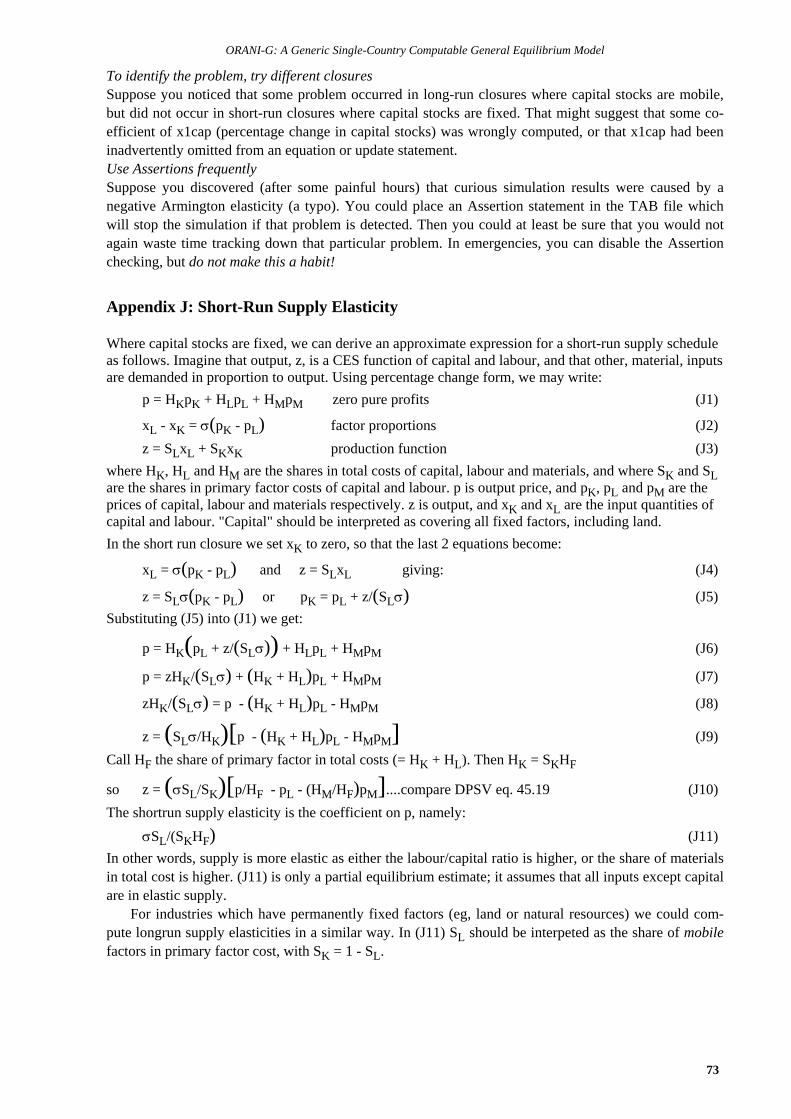
ORANI-G: A Generic Single-Country Computable General Equilibrium Model
73
To identify the problem, try different closuresSuppose you noticed that some problem occurred in long-run closures where capital stocks are mobile,but did not occur in short-run closures where capital stocks are fixed. That might suggest that some co-efficient of x1cap (percentage change in capital stocks) was wrongly computed, or that x1cap had beeninadvertently omitted from an equation or update statement.Use Assertions frequentlySuppose you discovered (after some painful hours) that curious simulation results were caused by anegative Armington elasticity (a typo). You could place an Assertion statement in the TAB file whichwill stop the simulation if that problem is detected. Then you could at least be sure that you would notagain waste time tracking down that particular problem. In emergencies, you can disable the Assertionchecking, but do not make this a habit!
Appendix J: Short-Run Supply Elasticity
Where capital stocks are fixed, we can derive an approximate expression for a short-run supply scheduleas follows. Imagine that output, z, is a CES function of capital and labour, and that other, material, inputsare demanded in proportion to output. Using percentage change form, we may write:
p = HKpK + HLpL + HMpM zero pure profits (J1)
xL - xK = (pK - pL) factor proportions (J2)
z = SLxL + SKxK production function (J3)
where HK, HL and HM are the shares in total costs of capital, labour and materials, and where SK and SLare the shares in primary factor costs of capital and labour. p is output price, and pK, pL and pM are theprices of capital, labour and materials respectively. z is output, and xK and xL are the input quantities ofcapital and labour. "Capital" should be interpreted as covering all fixed factors, including land.
In the short run closure we set xK to zero, so that the last 2 equations become:
xL = (pK - pL) and z = SLxL giving: (J4)
z = SL(pK - pL) or pK = pL + z/(SL) (J5)
Substituting (J5) into (J1) we get:
p = HK(pL + z/(SL)) + HLpL + HMpM (J6)
p = zHK/(SL) + (HK + HL)pL + HMpM (J7)
zHK/(SL) = p - (HK + HL)pL - HMpM (J8)
z = (SL/HK)[p - (HK + HL)pL - HMpM] (J9)
Call HF the share of primary factor in total costs (= HK + HL). Then HK = SKHF
so z = (SL/SK)[p/HF - pL - (HM/HF)pM]....compare DPSV eq. 45.19 (J10)
The shortrun supply elasticity is the coefficient on p, namely:
SL/(SKHF) (J11)
In other words, supply is more elastic as either the labour/capital ratio is higher, or the share of materialsin total cost is higher. (J11) is only a partial equilibrium estimate; it assumes that all inputs except capitalare in elastic supply.
For industries which have permanently fixed factors (eg, land or natural resources) we could com-pute longrun supply elasticities in a similar way. In (J11) SL should be interpeted as the share of mobilefactors in primary factor cost, with SK = 1 - SL.

Mark Horridge
74
Appendix K: List of Variables
Symbol Dimensions Description
a1(c,s,i) cCOM sSRC iIND Intermediate basic tech changea1_s(c,i) cCOM iIND Tech change, int'mdiate imp/dom compositea1cap(i) iIND Capital-augmenting technical changea1lab_o(i) iIND Labor-augmenting technical changea1lnd(i) iIND Land-augmenting technical changea1mar(c,s,i,m) cCOM sSRC iIND
mMAR Intermediate margin tech change
a1oct(i) iIND "Other cost" ticket augmenting techncal changea1prim(i) iIND All factor augmenting technical changea1tot(i) iIND All input augmenting technical changea2(c,s,i) cCOM sSRC iIND Investment basic tech changea2_s(c,i) cCOM iIND Tech change, investment imp/dom compositea2mar(c,s,i,m) cCOM sSRC iIND
mMAR Investment margin tech change
a2tot(i) iIND Neutral technical change - investmenta3(c,s) cCOM sSRC Household basic taste changea3_s(c) cCOM Taste change, household imp/dom compositea3lux(c) cCOM Taste change, supernumerary demandsa3mar(c,s,m) cCOM sSRC mMAR Household margin tech changea3sub(c) cCOM Taste change, subsistence demandsa4mar(c,m) cCOM mMAR Export margin tech changea5mar(c,s,m) cCOM sSRC mMAR Governmnt margin tech changecontBOT Contribution of BOT to real expenditure-side GDPcontGDPexp(e) eEXPMAC Contributions to real expenditure-side GDPdelB (Balance of trade)/GDPdelPTXRATE(i) iIND Change in rate of production taxdelSale(c,s,d) cCOM sSRC dDEST Sales aggregatesdelV0TAR(c) cCOM Ordinary change in tariff revenuedelV0tar_c Aggregate tariff revenuedelV0tax_csi Aggregate revenue from all indirect taxesdelV1CST(i) iIND Change in ex-tax cost of productiondelV1PRIM(i) iIND Ordinary change in cost of primary factorsdelV1PTX(i) iIND Ordinary change in production tax revenuedelV1PTX_i Ordinary change in all-industry production tax revenuedelV1TAX(c,s,i) cCOM sSRC iIND Interm tax revdelV1tax_csi Aggregate revenue from indirect taxes on intermediatedelV1TOT(i) iIND Change in tax-inc cost of productiondelV2TAX(c,s,i) cCOM sSRC iIND Invest tax revdelV2tax_csi Aggregate revenue from indirect taxes on investmentdelV3TAX(c,s) cCOM sSRC H'hold tax revdelV3tax_cs Aggregate revenue from indirect taxes on householdsdelV4TAX(c) cCOM Export tax revdelV4tax_c Aggregate revenue from indirect taxes on exportdelV5TAX(c,s) cCOM sSRC Govmnt tax revdelV5tax_cs Aggregate revenue from indirect taxes on governmentdelV6(c,s) cCOM sSRC Value of inventoriesdelx6(c,s) cCOM sSRC Inventories demandsemploy(i) iIND Employment by industryemploy_i Aggregate employment: wage bill weightsf0tax_s(c) cCOM General sales tax shifterf1lab(i,o) iIND oOCC Wage shift variablef1lab_i(o) oOCC Occupation-specific wage shifterf1lab_io Overall wage shifterf1lab_o(i) iIND Industry-specific wage shifter
.../continued

ORANI-G: A Generic Single-Country Computable General Equilibrium Model
75
Appendix K: List of Variables (continued)
Symbol Dimensions Description
f1oct(i) iIND Shift in price of "other cost" ticketsf1tax_csi Uniform % change in powers of taxes on intermediate usagef2tax_csi Uniform % change in powers of taxes on investmentf2tot Ratio, investment/consumptionf3tax_cs Uniform % change in powers of taxes on household usagef3tot Ratio, consumption/ GDPf4p(c) cCOM Price (upward) shift in export demand schedulef4p_ntrad Upward demand shift, Collective export aggregatef4q(c) cCOM Quantity (right) shift in export demandsf4q_ntrad Right demand shift, Collective export aggregatef4tax_ntrad Uniform % change in powers of taxes on nontradtnl exportsf4tax_trad Uniform % change in powers of taxes on tradtnl exportsf5(c,s) cCOM sSRC Government demand shiftf5tax_cs Uniform % change in powers of taxes on government usagef5tot Overall shift term for government demandsf5tot2 Ratio between f5tot and x3totfandecomp(c,f) cCOM fFANCAT Fan decompositionfinv1(i) iIND Shifter to enforce DPSV investment rulefinv2(i) iIND Shifter for "exogenous" investment rulefinv3(i) iIND Shifter for longrun investment rulefx6(c,s) cCOM sSRC Shifter on rule for stocksggro(i) iIND Gross growth rate of capital = Investment/capitalgret(i) iIND Gross rate of return = Rental/[Price of new capital]invslack Investment slack variable for exogenizing aggregate investmentp0(c,s) cCOM sSRC Basic prices for local usersp0cif_c Imports price index, C.I.F., local currencyp0com(c) cCOM Output price of locally-produced commodityp0dom(c) cCOM Basic price of domestic goods = p0(c,"dom")p0gdpexp GDP price index, expenditure sidep0gne GNE price indexp0imp(c) cCOM Basic price of imported goods = p0(c,"imp")p0imp_c Duty-paid imports price index, local currencyp0realdev Real devaluationp0toft Terms of tradep1(c,s,i) cCOM sSRC iIND Purchaser's price, intermediatep1_s(c,i) cCOM iIND Price, intermediate imp/dom compositep1cap(i) iIND Rental price of capitalp1cap_i Average capital rentalp1cst(i) iIND Index of production costs (for AnalyseGE)p1lab(i,o) iIND oOCC Wages by industry and occupationp1lab_io Average nominal wagep1lab_o(i) iIND Price to each industry of labour compositep1lnd(i) iIND Rental price of landp1lnd_i Average land rentalp1mat(i) iIND Intermediate cost price indexp1oct(i) iIND Price of "other cost" ticketsp1prim(i) iIND Effective price of primary factor compositep1tot(i) iIND Average input/output pricep1var(i) iIND Short-run variable cost price indexp2(c,s,i) cCOM sSRC iIND Purchaser's price, investmentp2_s(c,i) cCOM iIND Price, investment imp/dom compositep2tot(i) iIND Cost of unit of capitalp2tot_i Aggregate investment price indexp3(c,s) cCOM sSRC Purchaser's price, householdp3_s(c) cCOM Price, household imp/dom composite
.../continued

Mark Horridge
76
Appendix K: List of Variables (continued)
Symbol Dimensions Description
p3tot Consumer price indexp4(c) cCOM Purchaser's price, exports,loc$p4_ntrad Price, Collective export aggregatep4tot Exports price index, local currencyp5(c,s) cCOM sSRC Purchaser's price, governmentp5tot Government price indexp6tot Inventories price indexpe(c) cCOM Basic price of exportablespf0cif(c) cCOM C.I.F. foreign currency import pricespq1(c,i) cCOM iIND Price of output by commodity and industryphi Exchange rate, local currency/$worldq Number of householdsq1(c,i) cCOM iIND Output by commodity and industryrealwage Average real wageSalesDecomp(c,d) cCOM dDESTPLUS Sales decompositiont0imp(c) cCOM Power of tarifft1(c,s,i) cCOM sSRC iIND Power of tax on intermediatet2(c,s,i) cCOM sSRC iIND Power of tax on investmentt3(c,s) cCOM sSRC Power of tax on householdt4(c) cCOM Power of tax on exportt5(c,s) cCOM sSRC Power of tax on governmentutility Utility per householdw0cif_c C.I.F. local currency value of importsw0gdpexp Nominal GDP from expenditure sidew0gdpinc Nominal GDP from income sidew0gne Nominal GNEw0imp_c Value of imports plus dutyw0tax_csi Aggregate revenue from all indirect taxesw1cap_i Aggregate payments to capitalw1lab_io Aggregate payments to labourw1lnd_i Aggregate payments to landw1oct_i Aggregate "other cost" ticket paymentsw2tot_i Aggregate nominal investmentw3lux Total nominal supernumerary household expenditurew3tot Nominal total household consumptionw4tot Local currency border value of exportsw5tot Aggregate nominal value of government demandsw6tot Aggregate nominal value of inventoriesx0cif_c Import volume index, C.I.F. weightsx0com(c) cCOM Output of commoditiesx0dom(c) cCOM Output of commodities for local marketx0gdpexp Real GDP from expenditure sidex0gdpinc Real GDP from income sidex0gne Real GNEx0imp(c) cCOM Total supplies of imported goodsx0imp_c Import volume index, duty-paid weightsx0loc(c) cCOM Real percent change in LOCSALES (dom+imp)x1(c,s,i) cCOM sSRC iIND Intermediate basic demandsx1_s(c,i) cCOM iIND Intermediate use of imp/dom compositex1cap(i) iIND Current capital stockx1cap_i Aggregate capital stock, rental weightsx1lab(i,o) iIND oOCC Employment by industry and occupationx1lab_i(o) oOCC Employment by occupationx1lab_o(i) iIND Effective labour input
.../continued

ORANI-G: A Generic Single-Country Computable General Equilibrium Model
77
Appendix K: List of Variables (continued)
Symbol Dimensions Description
x1lnd(i) iIND Use of landx1lnd_i Aggregate land stock, rental weightsx1mar(c,s,i,m) cCOM sSRC iIND mMAR Intermediate margin demandx1oct(i) iIND Demand for "other cost" ticketsx1prim(i) iIND Primary factor compositex1prim_i Aggregate output: value-added weightsx1tot(i) iIND Activity level or value-addedx2(c,s,i) cCOM sSRC iIND Investment basic demandsx2_s(c,i) cCOM iIND Investment use of imp/dom compositex2mar(c,s,i,m) cCOM sSRC iIND
mMAR Investment margin demands
x2tot(i) iIND Investment by using industryx2tot_i Aggregate real investment expenditurex3(c,s) cCOM sSRC Household basic demandsx3_s(c) cCOM Household use of imp/dom compositex3lux(c) cCOM Household - supernumerary demandsx3mar(c,s,m) cCOM sSRC mMAR Household margin demandsx3sub(c) cCOM Household - subsistence demandsx3tot Real household consumptionx4(c) cCOM Export basic demandsx4_ntrad Quantity, Collective export aggregatex4mar(c,m) cCOM mMAR Export margin demandsx4tot Export volume indexx5(c,s) cCOM sSRC Government basic demandsx5mar(c,s,m) cCOM sSRC mMAR Government margin demandsx5tot Aggregate real government demandsx6tot Aggregate real inventories
List of Regional Variables
Symbol Dimensions Description
delregx6(c,s,r) cCOM sSRC rREG Inventories demandffreg1(i) iIND Complement of rsum1ffreg2(i) iIND Complement of rsum2ffreg3(c) cCOM Complement of rsum3ffreg4(c) cCOM Complement of rsum4ffreg5(c) cCOM Complement of rsum5ffreg6(c) cCOM Complement of rsum6freg1(i,r) iIND rREG Regional share shifterfreg2(i,r) iIND rREG Regional share shifterfreg3(c,r) cCOM rREG Regional share shifterfreg4(c,r) cCOM rREG Regional share shifterfreg5(c,r) cCOM rREG Regional share shifterfreg6(c,r) cCOM rREG Regional share shifterregadvantage(i,r) iIND rREG Reg advantage decompositionregemploy(i,r) iIND rREG Employment by reg and indregemploy_i(r) rREG Aggregate regional employmentregemploycon(i,r) iIND rREG Contributions to regional emplregw1lab_io(r) rREG Wage bills by regionregx0(c,r) cLOCCOM rREG Regional usage of local commoditiesregx1(c,s,i,r) cCOM sSRC iIND
rREG Regional demands for intermediate inputs
regx1mar(c,s,i,m,r) cCOM sSRC iINDmMAR rREG
Margins - production
regx1prim_i(r) rREG Gross region products
.../continued
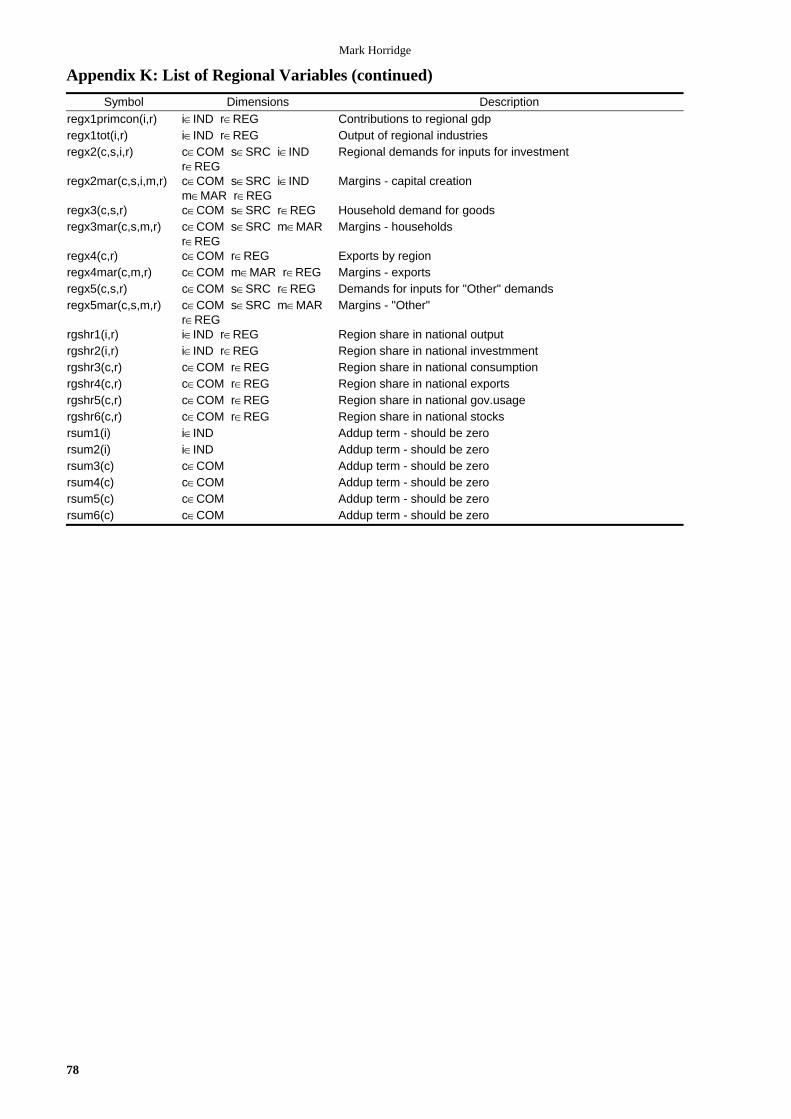
Mark Horridge
78
Appendix K: List of Regional Variables (continued)
Symbol Dimensions Description
regx1primcon(i,r) iIND rREG Contributions to regional gdpregx1tot(i,r) iIND rREG Output of regional industriesregx2(c,s,i,r) cCOM sSRC iIND
rREG Regional demands for inputs for investment
regx2mar(c,s,i,m,r) cCOM sSRC iINDmMAR rREG
Margins - capital creation
regx3(c,s,r) cCOM sSRC rREG Household demand for goodsregx3mar(c,s,m,r) cCOM sSRC mMAR
rREG Margins - households
regx4(c,r) cCOM rREG Exports by regionregx4mar(c,m,r) cCOM mMAR rREG Margins - exportsregx5(c,s,r) cCOM sSRC rREG Demands for inputs for "Other" demandsregx5mar(c,s,m,r) cCOM sSRC mMAR
rREG Margins - "Other"
rgshr1(i,r) iIND rREG Region share in national outputrgshr2(i,r) iIND rREG Region share in national investmmentrgshr3(c,r) cCOM rREG Region share in national consumptionrgshr4(c,r) cCOM rREG Region share in national exportsrgshr5(c,r) cCOM rREG Region share in national gov.usagergshr6(c,r) cCOM rREG Region share in national stocksrsum1(i) iIND Addup term - should be zerorsum2(i) iIND Addup term - should be zerorsum3(c) cCOM Addup term - should be zerorsum4(c) cCOM Addup term - should be zerorsum5(c) cCOM Addup term - should be zerorsum6(c) cCOM Addup term - should be zero