Optimizing the Performance of Sample

Mean-Variance Efficient Portfolios

Chris Kirby a, Barbara Ostdiek b

aBelk College of Business, University of North Carolina at CharlottebJones Graduate School of Business, Rice University

Abstract

We propose a comprehensive empirical strategy for optimizing the out-of-sample performanceof sample mean-variance efficient portfolios. After constructing a sample objective function thataccounts for the impact of estimation risk, specification errors, and transaction costs on portfo-lio performance, we maximize the function with respect to a set of tuning parameters to obtainplug-in estimates of the optimal portfolio weights. The methodology offers considerable flexibilityin specifying objectives, constraints, and modeling techniques. Moreover, the resulting portfo-lios have well-behaved weights, reasonable turnover, and substantially higher Sharpe ratios andcertainty-equivalent returns than benchmarks such as the 1/N portfolio and S&P 500 index.

Key words: active management, conditioning information, estimation risk, mean-varianceoptimization, portfolio choice, turnover

JEL classification: G11; G12; C11

July 23, 2012First draft: April 24, 2011

? Comments welcome. We thank Dejan Suskavcevic for excellent research assistance. A previousversion of the paper was circulated under the title ‘Optimal Active Portfolio Management with Un-conditional Mean-Variance Risk Preferences.” Address correspondence to: Chris Kirby, Departmentof Finance, Belk College of Business Administration, University of North Carolina at Charlotte,9201 University City Boulevard, Charlotte, NC 28223-0001.

1 Introduction

Empirical research on mean-variance portfolio optimization is typically conducted by substi-tuting estimates of the mean vector and covariance matrix of asset returns into an expressionfor the optimal portfolio weights. The portfolios constructed using this “plug-in” approachare called sample mean-variance efficient portfolios. Although the plug-in approach is con-ceptually straightforward, a number of implementation issues arise that fall outside the scopeof the optimization problem. These range from how to model changes in the investment op-portunity set and estimate the model parameters, to how to account for transaction costs.In this paper, we propose a methodology that encompasses the plug-in approach within abroader empirical framework that fully accounts for the impact of such issues on the perfor-mance of the plug-in weights. This allows us to optimize the out-of-sample performance ofsample mean-variance efficient portfolios with respect to specific investment objectives.

Our general empirical strategy is motivated by Skouras (2007). He suggests a decision-theoretic approach for estimating the parameters of any sufficiently regular rule that mapsrealizations of one or more random variables into decisions made by an economic agent. Theparameter estimates are obtained by maximizing an objective function that measures theeconomic benefit to the agent of following the given rule. In other words, the approach isdesigned to optimize the performance of the rule from an economic perspective. Brandt etal. (2009) provide a nice example of this approach applied in a portfolio choice setting. Theyinvestigate a parametric portfolio choice rule that restricts the portfolio weights to be linearin a set of asset-specific variables, such as size and book-to-market measures. To implementthe rule, they find the coefficients on the asset-specific variables that deliver the highestaverage utility for a specified historical sample period.

We use a similar methodology to optimize the performance of the plug-in approach. Thebasic strategy is as follows. First, we note that Ferson and Siegel (2001) derive an analyticexpression for the weights that deliver an unconditionally mean-variance efficient (UMVE)portfolio in settings with time-varying investment opportunities. This establishes the port-folio rebalancing rule that is optimal in the absence of estimation risk and rebalancing costs.Next, we use historical asset returns to construct plug-in weights that depend on a smallnumber of unknown parameters. This yields theoretically-motivated counterparts of the lin-ear weight functions used by Brandt et al. (2009). Finally, we use the plug-in weights togenerate a series of out-of-sample portfolio returns and find the values of the parametersthat maximize the mean return subject to a constraint on the return variance. Thus we fullyaccount for the impact of estimation risk when choosing the parameter values, and we cantake turnover into account simply by using returns measured net of rebalancing costs.

Ferson and Siegel (2001) show that the weights that deliver an UMVE portfolio are a func-tion of the conditional mean vector and conditional second-moment matrix of asset returns.Consistent with most studies in the portfolio choice literature, we focus on the case in whichthe conditioning information consists solely of past asset returns. For the empirical inves-tigation, we estimate the conditional moments of returns via simple exponential-smoothingmodels that emphasize parsimony and impose minimal assumptions about the data generat-ing process. Of course, using estimates in place of the true conditional moments introduces

1

estimation risk, i.e., uncertainty about portfolio returns that is incremental to the usual un-certainty about the individual asset returns. The presence of estimation risk complicates theportfolio choice problem because it affects the time-series properties of the plug-in weightsand, hence, the expected portfolio performance (see, e.g., Kan and Zhou, 2007).

To illustrate the nature of the complications, consider a scenario in which all investors formconditional expectations via exponential smoothing and use the same smoothing constant.Even if we use an exponential-smoothing model to estimate the conditional moments of assetreturns, the estimated optimal portfolio weights will generally deviate from the true weightsbecause the unknown value of the smoothing constant must either be specified a priori orestimated from the data. In either case, the potential for choosing an incorrect smoothingconstant causes the expected performance of the sample mean-variance efficient portfolio tofall short of the expected performance of the true optimal portfolio. Specification errors giverise to similar issues. If the models used to estimate the conditional moments of returns aremisspecified, the plug-in weights are not consistent estimates of the true optimal weights.The result is a decline in expected portfolio performance.

From an empirical point of view, the challenge is to minimize the adverse impact of estimationrisk and specification errors on portfolio performance. This argues for the use of specializedeconometric methods. Under a conventional econometric approach, choosing the smoothingconstants is a model-fitting problem. We might select the values that deliver the best forecastsof the returns and squared returns under mean-squared-error (MSE) loss. It is clear, however,that the model-fitting problem does not embody the same objective as the portfolio problem,which is to maximize expected utility under mean-variance risk preferences. Expected utilityfunctions generally translate into asymmetric loss functions, and asymmetric loss favorsestimates that are biased in an appropriate direction (Patton and Timmermann, 2007). Thevalues of the smoothing constants that deliver the best-performing portfolio could be quitedifferent from the values that minimize the MSE of the forecasts.

This insight lies at the core of our methodology. In effect, we treat any unknown parameterthat influences the time-series properties of the plug-in weights as a tuning parameter, i.e., asa parameter that can be freely changed to tailor portfolio performance to specific constraintsand objectives. In our framework, the goal is to maximize the unconditional expected returnon the portfolio subject to a constraint on the unconditional return variance. We thereforeselect the model parameters based on the sample moments of the sequence of out-of-sampleportfolio returns that result from using historical data to construct a time series of plug-in portfolio weights. Specifically, we find the parameter values that generate the highestaverage realized utility under mean-variance risk preferences. This optimizes the out-of-sample performance of the portfolio.

The proposed approach is not restrictive in terms of either modeling techniques or constraintson portfolio holdings. For example, we consider sample UMVE portfolios constructed usingshrinkage estimators of the conditional moments of returns. The shrinkage factor is there-fore included as an additional tuning parameter to be estimated in conjunction with othermodel parameters. We also address issues of portfolio turnover and rebalancing costs byexplicitly accounting for the effect of turnover in the tuning-parameter optimization. Thisis accomplished by using returns measured net of rebalancing costs to construct the sam-

2

ple objective function. The approach can easily be extended to incorporate techniques forreducing turnover and the attendant rebalancing costs.

For example, Leland (1999) argues that partial-adjustment strategies are the appropriateway to deal with rebalancing costs. These strategies recognize that costly trading can makeit inefficient to fully adjust to the estimated optimal weights each period. We develop apartial-adjustment strategy that defines a no-trade region around the estimated optimalweights each period using an estimate of the conditional expected utility loss from leavingthe weights unchanged. If this loss is less than some cutoff, no adjustment is made; otherwisethe existing weights are adjusted to the no-trade boundary. We estimate the optimal size ofthe no-trade region by including the cutoff in the set of tuning parameters.

We evaluate the effectiveness of the proposed methodology for three datasets that containmonthly returns on equally-weighted U.S. equity portfolios. Using portfolios as assets insteadof individual stocks is common in research on mean-variance optimization. We do so becauseit allows us to assess the potential for exploiting well-known empirical regularities such asvalue, growth, and momentum effects. The first two datasets are the Fama-French 10 Industryportfolios and 25 Size/Book-to-Market portfolios. To construct the third dataset, we sortNYSE, AMEX, and NASDAQ firms into 30 Momentum/Volatility portfolios using theirpast returns and average absolute returns. The sample period is January 1946 to December2009. We reserve the first 360 months of data to construct the plug-in weights for the initialinvestment period, leaving 408 months for performance evaluation.

To generate our empirical results, we maximize average realized utility under mean-variancerisk preferences using a relative risk aversion of 15. This level of risk aversion imposes asubstantial risk penalty, producing a relatively conservative investment style. The analysisreveals that our methodology performs well along a number of dimensions. For instance, ifwe estimate the optimal values of the tuning parameters and measure portfolio performanceassuming proportional transaction costs of 50 basis points (bp), then the sample UMVEportfolio for the 10 Industry dataset has an estimated Sharpe ratio of 0.94. In comparison,the S&P 500 index and the 1/N portfolio have estimated Sharpe ratios of 0.41 and 0.54. Theperformance advantage of the sample UMVE portfolio is highly statistically significant andpoints to substantial benefits from employing mean-variance optimization.

This finding is tempered, however, by the high level of turnover required to realize thesebenefits. It averages over 380% per year. In an effort to reduce the turnover of the portfolio,we explore the use of partial adjustment techniques. This meets with only modest success forthis dataset. Allowing for partial adjustment of the weights decreases the average turnover ofthe sample UMVE portfolio by only about 45 percentage points per year. The high turnoveris probably related to the low cross-sectional dispersion in average returns for the 10 Industrydataset — a characteristic not shared with the other two datasets. Because there is littlecross-sectional variation in the sample means, the performance gains may largely reflect thesuccess of the optimizer in exploiting, by what turns out to be aggressive rebalancing, thetime-series variation in conditional expected returns.

The results for the 25 Size/Book-to-Market and 30 Momentum/Volatility datasets are consis-tent with this hypothesis in the sense that turnover is of less concern. Under the same 50 bp

3

transaction costs assumption, the sample UMVE portfolios for these datasets have estimatedSharpe ratios of 0.95 and 1.46, respectively. The average turnover for the 25 Size/Book-to-Market dataset is 286% per year, which is still relatively high. But the average turnover isconsiderably lower for the 30 Momentum/Volatility dataset: 158% per year. With partialadjustment of the weights, these figures fall to 137% and 75%, respectively. This drop inaverage turnover is accompanied by an increase in the estimated Sharpe ratios of the sampleUMVE portfolios to 1.03 and 1.54. In comparison, the 1/N portfolio generates an estimatedSharpe ratio of about 0.57 for both datasets.

Taking the effort to reduce turnover a step further, we combine partial adjustment of theweights with the use of shrinkage estimators while simultaneously imposing a long-onlyconstraint. We find that prohibiting short sales leads to a considerable reduction in theestimated Sharpe ratios. For example, the long-only sample UMVE portfolio for the 30 Mo-mentum/Volatility dataset has an estimated Sharpe ratio of 1.04. It is noteworthy, however,that this portfolio outperforms all of the benchmarks at the 1% significance level, and it doesso despite having an average turnover of only 8% per year. Thus prohibiting short sales is aneffective strategy for sharply reducing turnover, and it allows the sample UMVE portfoliosto maintain a significant performance advantage over the benchmarks.

Overall the empirical evidence suggests that the proposed methodology leads to robust port-folio selection rules. It achieves robustness by expanding the scope of the optimization prob-lem to encompass the effects of estimation risk, specification errors, and transaction costson portfolio performance, and using an adaptive empirical strategy to select the values ofthe unknown parameters that appear in the expression for the plug-in weights. This is incontrast to the ad hoc strategies for selecting the values of these parameters considered else-where in the literature. Although researchers have long recognized that the performance ofmean-variance optimization is sensitive to the choice of parameter values, there is a dearthof research on choosing these values in a robust fashion. The empirical strategy developedhere represents a significant step forward in this regard.

2 Methodology for Optimizing the Performance of Sample UMVE Portfolios

The analysis is framed in terms of the portfolio problem of an investor who wants to rebalancehis portfolio on a regular basis to take advantage of time-varying investment opportunities.We assume that the rebalancing process is accomplished using a formal rule that specifieshow the portfolio weights respond to changes in the investment opportunity set. To identifythe optimal rebalancing rule, we have to specify a well-defined investment objective. Weanalyze the case in which the objective is to maximize the unconditional expected returnof the portfolio subject to a constraint on the unconditional portfolio variance. That is, weassume the goal is to construct a UMVE portfolio.

Although it is somewhat unusual to specify an unconditional investment objective in a set-ting with time-varying investment opportunities, this is consistent with the common practiceof unconditional performance evaluation. Mutual fund ratings, for example, are largely deter-mined by fund performance over an extended interval such as three or five years. Portfoliosconstructed using conditional objectives may fare poorly if their performance is evaluated

4

from an unconditional perspective (Dybvig and Ross, 1985). Of course, unconditional op-timization is a special case of conditional optimization in our framework, because everyUMVE portfolio is also conditionally mean-variance efficient (Hansen and Richard, 1987).We emphasize the unconditional representation of the portfolio problem because uncondi-tional optimization with respect to a set of tuning parameters plays a key role in the analysis.

2.1 UMVE portfolios with time-varying investment opportunities

Ferson and Siegel (2001) provide a general characterization of the set of active portfoliostrategies that deliver minimum-variance portfolios in the presence of time-varying invest-ment opportunities. Suppose for illustration purposes that there are N risky assets. Let rt+1

denote the N × 1 vector of asset returns for period t + 1 and let rp,t+1 = w′trt+1 denote the

portfolio return for period t+ 1, where wt is an N × 1 vector of weights selected in period tthat sum to 1. Ferson and Siegel (2001) show that the weights that produce the minimumvalue of σ2

p = Var(rp,t+1) for a given value of µp = E[rp,t+1] are of the form

wt =Ω−1

t ι

ι′Ω−1t ι

+µp − µp0

µp1 − µp0

(Ω−1

t − Ω−1t ιι′Ω−1

t

ι′Ω−1t ι

)µt ∀t, (1)

where µt = Et[rt+1] is the conditional mean vector of returns, Ωt = Et[rt+1r′t+1] is the

condition second moment matrix of returns,

µp0 = E

[ι′Ω−1

t µt

ι′Ω−1t ι

], (2)

µp1 = E

[µ′tΩ

−1t µt + (1− ι′Ω−1

t µt)ι′Ω−1

t µt

ι′Ω−1t ι

], (3)

and ι is an N × 1 vector of ones. The scalars µp0 and µp1 denote the expected returns oftwo portfolios on the minimum-variance frontier: the portfolio with the minimum value ofEt[r

2p,t+1] and the portfolio with the maximum value of Et[rp,t+1]− (1/2)Et[r

2p,t+1].

Equation (1) implies that we can construct the minimum-variance portfolio for a targetexpected return of µp by investing a fraction of wealth, xp = (µp − µp0)/(µp1 − µp0), in thefrontier portfolio with expected return µp1 and the remainder in the frontier portfolio withexpected return µp0 . This construction is not unique because any two frontier portfolios spanthe entire minimum-variance frontier (Hansen and Richard, 1987). However, it is the onlyconstruction for which the weights of the two spanning portfolios can be expressed in termsof µt and Ωt alone, i.e., without the use of any scaling constants.

Setting µp ≥ µp0/(1 − µp1 + µp0) delivers a UMVE portfolio (Ferson and Siegel, 2001). Tosee this, consider the problem of choosing wt to maximize the quadratic objective function

Qp(wt) = E[w′trt+1]−

γ

2Var(w′

trt+1), (4)

where γ > 0. The solution clearly delivers a UMVE portfolio because it maximizes E[rp,t+1]for some value of Var(rp,t+1). Moreover, the solution must be of the form shown in equation

5

(1) because maximizing Qp(wt) subject to E[rp,t+1] = µp also minimizes Var(rp,t+1) subjectto E[rp,t+1] = µp.

Substituting equation (1) into equation (4) and applying the law of iterated expectationsyields the concentrated objective function

Qp(µp) = µp −γ

2

(E[(ι′Ω−1

t ι)−1] +(µp − µp0)

2

µp1 − µp0

− µ2p

)(5)

with µp as the choice variable. Using equation (5) we find that Qp(wt) is maximized for

µp =µp0

1− µp1 + µp0

+1

γ

(µp1 − µp0

1− µp1 + µp0

). (6)

Hence, we have µp ≥ µp0/(1− µp1 + µp0) for a UMVE portfolio.

In the subsequent analysis we exploit the close connection between the problem of findinga UMVE portfolio and the problem of maximizing expected utility under quadratic riskpreferences. To see the connection, suppose someone with utility of the form

U(wt) = w′trt+1 −

ψ

2(w′

trt+1)2 (7)

wants to maximize E[U(wt)]. Because maximizing E[U(wt)] subject to E[rp,t+1] = µp isequivalent to minimizing Var(rp,t+1) subject to E[rp,t+1] = µp, it again follows that thesolution must be of the form shown in equation (1).

Substituting equation (1) into equation (7) and applying the law of iterated expectationsyields the concentrated objective function

E[U(µp)] = µp −ψ

2

(E[(ι′Ω−1

t ι)−1] +(µp − µp0)

2

µp1 − µp0

), (8)

which is maximized for µp = µp0 + (µp1 − µp0)/ψ. Hence, we obtain

wt =Ω−1

t ι

ι′Ω−1t ι

+1

ψ

(Ω−1

t − Ω−1t ιι′Ω−1

t

ι′Ω−1t ι

)µt (9)

as the optimal vector of weights. This is the same vector of weights that maximizes

Et[U(wt)] = w′tµt −

ψ

2w′

tΩtwt (10)

subject to w′tι = 1. Setting ψ = γ(1− µp1 + µp0)/(1 + γµp0) delivers the UMVE portfolio for

a given value of γ. Note that we have ψ < γ because µp1 > µp0 > 0.

2.2 Plug-in estimation of the optimal weights

Equation (1) is derived under the assumption that the values of µp0 , µp1 , µt, and Ωt are known.Because this assumption is not satisfied in practice, we follow the related empirical literature

6

by using the plug-in approach to implement the Ferson and Siegel (2001) methodology. Thatis, we use historical data to estimate the unknown parameters, and substitute the parameterestimates into the formula for the optimal portfolio weights. Using estimates in place of thepopulation parameters entails estimation risk: uncertainty about portfolio returns that isincremental to the uncertainty about individual asset returns. 1 It is important, therefore,to consider the impact of this risk on portfolio performance.

The empirical investigation focuses on the case in which the conditioning information consistssolely of historical returns. We refer to the sample of returns ending at T0 as the initial“holdout” sample. To use this sample to construct plug-in weights for the interval T0 toT0 + 1, we must first specify estimators for µT0 and ΩT0 . Many methods could be usedto model the conditional moments of returns. We employ a simple filtering technique thatemphasizes parsimony and imposes minimal assumptions about the data generating process.In particular, we specify exponentially-weighted rolling estimators of the form

µT0(φ) =

T0∑t=1

φT0−t

−1T0∑t=1

φT0−trt (11)

ΩT0(ϕ) =

T0∑t=1

ϕT0−t

−1T0∑t=1

ϕT0−trtr′t (12)

where the smoothing constants φ and ϕ satisfy 0 < φ,ϕ ≤ 1.

The use of rolling estimators is common in research on mean-variance portfolio selection.A number of studies, for example, construct plug-in estimates of the portfolio weights byusing a fixed-width rolling data window to estimate the mean vector and covariance matrixof asset returns. 2 This approach seeks to balance the benefits of increasing the sample sizeagainst the costs of including more distant observations that are less likely to reflect currentmarket conditions. Although the use of a fixed-width window has some intuitive appeal, it istypically less efficient than methods that exploit the full historical sample of asset returns.The literature suggests that exponentially-weighted rolling estimators are preferred from anefficiency perspective (see, e.g., Foster and Nelson, 1996).

Developing a robust method for choosing the smoothing constants is central to our investi-gation. One possibility is to use a model-fitting approach. For instance, we might choose the

1 This motivates Paye (2010) to propose a methodology in which multiple plug-in estimates of theweights are combined to obtain the final weights. He shows how to estimate the combination thatminimizes the investor’s expected loss, but finds that it is more robust to use a simple average ofthe different plug-in estimates because this entails less estimation risk overall.2 Some recent examples include DeMiguel et al. (2009), Paye (2010), Tu and Zhou (2011), andKirby and Ostdiek (2012).

7

smoothing constants by minimizing sample criteria of the form

G(φ) = tr

1

T0 − 1

T0−1∑t=1

(rt+1 − µt(φ))(rt+1 − µt(φ))′

, (13)

H(ϕ) = tr

1

T0 − 1

T0−1∑t=1

(rt+1r′t+1 − Ωt(ϕ))(rt+1r

′t+1 − Ωt(ϕ))′

, (14)

where tr· denotes the trace operator. This would deliver estimates of the values of φ andϕ that produce the best forecasts of the returns and their squares and cross products underMSE loss. In general, however, we would not expect such an approach to be satisfactory,because the values that minimize G(φ) and H(ϕ) are unlikely to coincide with the valuesthat optimize the performance of the portfolio. The same is true for any approach that relieson an econometrically-motivated loss function. 3

We can see this more clearly by considering the implications of specifying risk preferences ofthe form shown in equation (7). Under a model-fitting approach, we can express the vectorof plug-in weights for period T0 as

wT0(ψ, φ, ϕ) =Ω−1

T0(ϕ)ι

ι′Ω−1T0

(ϕ)ι+

1

ψ

Ω−1T0

(ϕ)−Ω−1

T0(ϕ)ιι′Ω−1

T0(ϕ)

ι′Ω−1T0

(ϕ)ι

µT0(φ), (15)

where φ = g(r1, r2, . . . , rT0) and ϕ = h(r1, r2, . . . , rT0) for some model-specific functions g(·)and h(·). The optimal vector of weights, on the other hand, can be expressed as

wT0(ψ) =1

ψΩ−1

T0(µT0 − κT0(ψ)ι), (16)

where κT0(ψ) = (ψ − ι′Ω−1T0µT0)/ι

′Ω−1T0ι.

If we substitute equation (15) into the utility function in equation (7) and take conditionalexpectations, we obtain

ET0 [U(wT0(·))] = κT0(ψ) + ψwT0(ψ)′ΩT0wT0(ψ, φ, ϕ)− ψ

2wT0(ψ, φ, ϕ)′ΩT0wT0(ψ, φ, ϕ). (17)

In comparison, substituting equation (16) into the utility function in equation (7) and takingconditional expectations yields

ET0 [U(wT0(·))] = κT0(ψ) +ψ

2wT0(ψ)′ΩT0wT0(ψ). (18)

Hence, under the utility-based loss function

L(wT0 , wT0) = U(wT0(·))− U(wT0(·)), (19)

3 If we consider the case in which rt ∼ i.i.d. N (µ,Σ), for example, using the maximum likelihoodestimators of µ and Σ to construct the plug-in weights does not maximize the expected out-of-sample performance of the portfolio (Kan and Zhou, 2007).

8

the conditional expected loss is

ET0 [L(wT0 , wT0)] =ψ

2(wT0(ψ)− wT0(ψ, φ, ϕ))′ΩT0(wT0(ψ)− wT0(ψ, φ, ϕ)) (20)

by using the plug-in weights in place of the optimal weights. The unconditional expectedloss follows immediately by the law of iterated expectations.

It is apparent from equation (20) that the magnitude of the expected loss from using theplug-in weights depends on the nature of the functions g(·) and h(·). Under a model-fittingapproach these functions are defined implicitly by solving for the values of φ and ϕ thatmaximize goodness-of-fit with respect to standard statistical criteria. In general, there is noguarantee that the resulting estimators deliver a small expected utility loss. To develop adecision-theoretic approach for choosing the smoothing constants, we treat them as tuningparameters, i.e., as parameters that we can freely change to tailor the performance of theplug-in weights to a particular investment objective.

2.3 Estimating the optimal values of the tuning parameters

Suppose we want to use the Ferson and Siegel (2001) framework to construct a sample UMVEportfolio. Under these circumstances, the problem is to select an active portfolio strategyfrom within the set of strategies that have weights of the form

wT0(ϑ) =Ω−1

T0(ϕ)ι

ι′Ω−1T0

(ϕ)ι+

1

ψ

Ω−1T0

(ϕ)−Ω−1

T0(ϕ)ιι′Ω−1

T0(ϕ)

ι′Ω−1T0

(ϕ)ι

µT0(φ). (21)

where ϑ = (ψ, φ, ϕ)′ denotes the vector of tuning parameters. To identify the optimal activestrategy under unconditional mean-variance risk preferences, we have to find the value of ϑthat maximizes the quadratic objective function

Qp(ϑ) = E[wT0(ϑ)′rT0+1]−γ

2Var(wT0(ϑ)′rT0+1), (22)

where γ measures relative risk aversion. If we assume that µT0(φ) and ΩT0(ϕ) are correctly-specified parametric models of the conditional mean vector and conditional second-momentmatrix, then Qp(ϑ) is maximized by setting ψ = γ(1− µp1 + µp0)/(1 + γµp0), and choosing

φ and ϕ such that µT0(φ) = µT0 and ΩT0(ϕ) = ΩT0 . This yields the same vector of weightsas maximizing Qp(wt) in equation (4) for t = T0.

The value of ϑ that maximizes Qp(ϑ) is unknown in practice. However, we can use historicalreturns to construct a sample version of the objective function and estimate this value in astraightforward fashion. To implement our estimation methodology, we split the initial hold-out sample into an “initialization window” that contains the first K0 ≥ N observations andan “estimation window” that contains the remaining T0−K0 observations. 4 The returns inthe initialization window are used to initialize the rolling estimators of the conditional mean

4 The restriction K0 ≥ N is imposed to ensure that the estimate of Ωt is invertible for all t ≥ K0,i.e., for all dates contained in the estimation window.

9

vector and conditional second-moment matrix, and the returns in the estimation window areused to construct the sample objective function and estimate the optimal value of ϑ.

The proposed estimator is obtained by applying the weights wt(ϑ)T0−1t=K0

to the returns inthe estimation window. Note that wt(ϑ) depends only on the returns observed in periods 1through t. It follows, therefore, that applying wt(ϑ) to rt+1 delivers an out-of-sample portfolioreturn for period t + 1. For any choice of ϑ, the sample mean and sample variance of theout-of-sample portfolio returns for the estimation window are given by

µp(ϑ) =1

T0 −K0

T0−1∑t=K0

wt(ϑ)′rt+1, (23)

σ2p(ϑ) =

1

T0 −K0

T0−1∑t=K0

(wt(ϑ)′rt+1 − µp(ϑ))2. (24)

These sample moments are analogs of the population moments that appear on the right sideof equation (22). Under suitable regularity conditions, therefore, the estimate of ϑ obtainedby maximizing the sample objective function

Qp(ϑ) = µp(ϑ)− γ

2σ2

p(ϑ) (25)

converges as T0 −K0 →∞ to the value of this vector that maximizes Qp(ϑ). 5

In general, we expect the sample objective function to be constructed using misspecifiedeconometric models. For example, the volatility modeling literature suggests that even forsmall values of N we need a heavily-parameterized model to fully capture the dynamics of Ωt.Such a model may not be practical in portfolio-choice applications. If we instead use a moreparsimonious specification, such as the rolling estimator considered here, the plug-in weightswill differ from the true weights for all possible values of the tuning parameters. In this case,maximizing the sample objective function yields estimates of the values of tuning parametersthat deliver a portfolio that is UMVE with respect to the choice set established by using themisspecified models to construct the plug-in weights. This yields the most efficient portfoliopossible given the choice of modeling techniques.

We also expect the estimates of φ and ϕ obtained by maximizing Qp(ϑ) to serve the un-derlying investment objectives better than either ad hoc choices of the parameter valuesor the estimates obtained from a model-fitting approach. To understand why, note thatour approach maximizes the average realized utility generated by the portfolio as opposedto a statistical goodness-of-fit criterion. Because utility-based objective functions generallytranslate into asymmetric loss functions, overestimating an expected return or variance willtypically produce a different loss than underestimating this quantity by the same amount.

5 Note that global identification is not a concern in this setting, because our objective is limitedto constructing an estimate of ϑ that converges to the value that maximizes Qp(ϑ) as T0 −K0 →∞. There is no need to assume that the maximum of Qp(ϑ) corresponds to a unique parameterconfiguration. For a detailed discussion of identification in the context of parameter estimationusing economic loss functions, see Skouras (2007).

10

As a consequence, the tuning-parameter optimization favors estimates of φ and ϕ that arebiased in an appropriate direction. 6

By estimating φ and ϕ jointly with ψ, we allow the optimizer to fully evaluate all of thetradeoffs involved in choosing the tuning parameter values. For instance, reducing the valueof φmight produce more accurate estimates of conditional expected returns, but it might alsoincrease the time-series variation in the plug-in weights. In isolation this could be counterpro-ductive. However, increasing the value of ψ might compensate for the increased variation inthe plug-in weights and ultimately produce a higher value of the sample objective function.Assessing the potential for such tradeoffs is at the core of our strategy for identifying tuningparameter values that optimize the out-of-sample performance of the portfolio. 7

Brandt et al. (2009) use a related estimation strategy to implement a parametric portfo-lio rule in large-scale applications. Under their approach, each asset weight is restricted tobe linear in a set of asset-specific variables, such as market capitalization, book-to-marketvalue, and lagged returns. This linear-weight-function approach is a middle ground betweena fully-specified model of optimal portfolio choice and pure technical trading rules. Althoughit is an approximation, it has the advantage of drastically reducing computational demandswhen N is large by eliminating the need to estimate the optimal weights using the functionalform implied by theory. Because the values of coefficients in the linear weight functions areunknown, Brandt et al. (2009) estimate them from the data. In particular, they find the coef-ficient values that maximize average utility over their sample period under a specified utilityof wealth function. The proposed approach for optimizing the out-of-sample performance ofthe plug-in weights is a theory-based alternative to their methodology.

2.4 Portfolio turnover and rebalancing costs

Portfolio turnover is always a concern if transaction costs are greater than zero. In thissituation, anything that increases turnover can decrease performance after accounting forrebalancing costs. Turnover is usually defined as the fraction of invested wealth traded in agiven period to rebalance the portfolio. To see how to compute this measure, note that if onedollar is invested in the portfolio in period t− 1, there are wi,t−1(ϑ)(1 + ri,t) dollars investedin the ith asset of the portfolio in period t. Hence, the weight in asset i before the portfolio

6 Using asymmetric loss functions to evaluate forecast quality is an area of ongoing research. Underasymmetric loss, many of the properties traditionally associated with forecast optimality need nothold. Optimal forecasts can be biased, the forecast errors can display arbitrarily high orders of serialcorrelation, and the variance of the forecast errors can decline as the forecast horizon increases(Patton and Timmermann, 2007).7 In our experience, the sample objective function in equation (25) tends to have a number oflocal optima, so some care is needed to avoid termination of the optimization algorithm at thesepoints. We guard against this possibility by conducting multiple optimizations using a range ofstarting values. Despite this precaution, there may be some cases in which we fail to find the globaloptimum. Our analysis suggests, however, that the remaining improvement in the value of theobjective function that could be achieved in such cases is very small.

11

is rebalanced is

wi,t(ϑ) =wi,t−1(ϑ)(1 + ri,t)

1 +∑N

i=1 wi,t−1(ϑ)ri,t

, (26)

and the turnover at time t is given by

τp,t(ϑ) =1

2

N∑i=1

|wi,t(ϑ)− wi,t(ϑ)|, (27)

where wi,t(ϑ) is the desired weight in asset i at time t. 8

One advantage of the proposed methodology is that we can take turnover and rebalancingcosts directly into account. To illustrate, let rp,t denote the portfolio return net of rebalancingcosts for period t. Now suppose that the cost of rebalancing the portfolio to the desired periodt weights is subtracted from the return for period t, and that the level of transaction costsis constant both across assets and over time. Under these circumstances,

rp,t(ϑ) = (1 + w′t−1(ϑ)rt)(1− 2τp,t(ϑ)c)− 1, (28)

where c is the assumed level of proportional costs per transaction. 9 We can therefore estimatethe optimal values of the tuning parameters for a given c by using rp,t(ϑ)K0

t=1 to initializethe rolling estimators and rp,t(ϑ)T0

t=K0+1 to construct the sample objective function. Theassumption that c is constant could easily be relaxed. For instance, evidence suggests thatthe cost of trading U.S. equities has declined over time (Domowitz et al., 2001; Hasbrouck,2009). This decline can be captured by specifying a linear time trend for trading costs of theform ct = c0 + c1t with appropriate values of c0 and c1.

2.5 Shrinkage and partial-adjustment techniques

Shrinkage methods are a popular technique for improving the performance of the plug-inapproach to constructing portfolio weights. The basic idea of shrinkage estimators, as firstdescribed by James and Stein (1961), is to reduce the extreme estimation errors that mayoccur when estimating the cross-section of means, variances, and covariances of asset returns.For example, we might shrink the sample mean for each asset towards the grand sample meanfor all the assets. This mitigates the largest estimation errors and may reduce the varianceof the estimators by enough to outweigh the biases introduced by the technique.

It is straightforward to apply shrinkage methods in the proposed framework. Consider esti-

8 Equation (27) is consistent with the measure of turnover used in the mutual fund industry, i.e.,the lesser of the value of purchases and sales in the period divided by net asset value. Here thevalue of purchases equals the value of sales because there are no fund inflows or outflows.9 Note that τp,t(ϑ) is multiplied by 2 in equation (28) because turnover is the value of assetspurchased or, equivalently in our framework, the value of assets sold as a fraction of total wealth.Both purchases and sales incur transaction costs, so rebalancing costs are given by 2τp,t(ϑ)c.

12

mators for µt and Ωt of the form

µ∗t (φ, ρ) = ρµt + (1− ρ)µt(φ), (29)

Ω∗t (ϕ, ρ) = ρΩt + (1− ρ)Ωt(ϕ), (30)

where µt and Ωt are the shrinkage targets and the shrinkage factor ρ satisfies 0 < ρ ≤ 1. 10

Consistent with the general approach, we treat ρ as a tuning parameter. Thus the vector ofplug-in weights for period t becomes

w∗t (ϑ

∗) =Ω∗−1

t (ϕ, ρ)ι

ι′Ω∗−1t (ϕ, ρ)ι

+1

ψ

(Ω∗−1

t (ϕ, ρ)− Ω∗−1t (ϕ, ρ)ιι′Ω∗−1

t (ϕ, ρ)

ι′Ω∗−1t (ϕ, ρ)ι

)µ∗t (φ, ρ), (31)

where ϑ∗ = (ϑ′, ρ)′ contains the original tuning parameters plus the shrinkage factor. Theshrinkage targets are obtained by averaging the sample means, sample second moments, andsample second moments of the returns that are in the investor’s information set when theweights are selected. Specifically, we set µit = ι′µt(1)/N for all i, Ωii,t = trΩt(1)/N for all

i, and Ωij,t = (ι′Ωt(1)ι− trΩt(1))/(N2 −N) for all i 6= j.

The empirical evidence suggests that shrinkage methods reduce the adverse impact of esti-mation risk, but they may not be the most effective way to address the issue of rebalancingcosts. For this reason, we also consider partial-adjustment strategies. These strategies rec-ognize that costly trading can make it inefficient to fully adjust to the estimated optimalposition each period because there is an inherent tradeoff between the benefits of incor-porating information about changes in the investment opportunity set and the attendantrebalancing costs. The idea behind partial-adjustment strategies is to strike an appropriatebalance between these costs and benefits.

Brandt et al. (2009) propose one such strategy. They use a function of the form

dt(δ) =1

N

N∑i=1

(wi,t − w∗i,t(δ))

2 (32)

to measure the distance between the desired weights, wt, and weights before any rebalancingoccurs, w∗

t (δ), and specify that no adjustment of the weights takes place if dt(δ) ≤ δ. Thusthere is a no-trade region — a hypersphere of radius

√δ — around wt. For cases in which

dt(δ) > δ, the weights are adjusted to the boundary of the no-trade region by setting

w∗t (δ) = %t(δ)w

∗t (δ) + (1− %t(δ))wt, (33)

where %t(δ) = (δ/dt(δ))1/2.

Although partial-adjustment strategies can be motivated by the theory of portfolio optimiza-tion in the presence of transaction costs (see, e.g., Leland, 1999), there is no claim that theoptimal shape of the no-trade region is a hypersphere. Indeed, equation (20) suggests using adifferent shape for an investor with quadratic risk preferences. It shows that the conditional

10 We investigated using different shrinkage factors for the first and second moments, but foundthat this had little impact on our results.

13

expected loss generated by errors in estimating the optimal weights is a quadratic form in theconditional second moment matrix of returns. Accordingly, we propose a partial-adjustmentstrategy based on the distance measure

dt(ϑ∗) = (wt(ϑ)− w∗

t (ϑ∗))′Ωt(ϕ)(wt(ϑ)− w∗

t (ϑ∗)), (34)

where ϑ∗ = (ϑ′, δ)′ contains the original tuning parameters plus the no-trade distance. Thevalue of dt(ϑ

∗) approximates the conditional expected loss in utility from leaving the weightsunchanged. If the anticipated loss is less than δ, no adjustment takes place. Otherwise theweights are adjusted to the no-trade boundary by setting

w∗t (ϑ

∗) = %t(ϑ∗)w∗

t (ϑ∗) + (1− %t(ϑ

∗))wt(ϑ), (35)

where %t(ϑ∗) = (δ/dt(ϑ

∗))1/2.

3 Empirical Application

To investigate the effectiveness of the proposed methodology, we consider an empirical ap-plication in which the goal is to create an optimal “fund-of-funds” strategy by investing ina defined set of characteristic-based portfolios that contain NYSE, AMEX, and NASDAQfirms. Using portfolios rather than individual stocks as assets has two advantages. First, itallows us to assess the extent to which the cross-sectional and time-series variation in theplug-in weights is related to well-known empirical regularities, such as value, growth, andmomentum effects. This provides insights on the features of the research design that influencethe performance of sample UMVE portfolios. Second, it allows us to directly relate our find-ings to the literature, because most of the empirical research on mean-variance optimizationuses portfolios rather than individual stocks.

We use a number of equity benchmarks, such as the S&P 500 index, to draw inferences aboutthe observed performance of the sample UMVE portfolios. Treasury bills are excluded fromthe set of assets to ensures that the observed differences in performance between the sampleUMVE portfolios and the benchmarks are not driven by allocations to the conditionally risk-free security. As Brandt et al. (2009) point out, the first-order effect of including a risk-freesecurity in the portfolio is simply to change the leverage, not the relative weightings of therisky assets. Thus, little is lost by excluding Treasury bills from consideration.

3.1 Datasets

The empirical investigation is conducted using monthly returns on three sets of equally-weighted stock portfolios for the period from January 1946 to December 2009 (768 observa-tions). 11 We employ equally-weighted portfolios for the analysis so that naıve diversification,one of our benchmark strategies, corresponds to holding an equally-weighted portfolio of in-dividual stocks. This allows us to attribute the observed differences in performance between

11 We exclude data prior to 1945 from the analysis because of the atypical conditions that prevailedin U.S. equity markets during the Great Depression and World War II.

14

the 1/N portfolio and the sample UMVE portfolios to the impact of grouping individualfirms on the basis of observed characteristics and using mean-variance optimization to takeadvantage of the resulting cross-sectional and time-series variation in the conditional mo-ments of returns. In general, we expect the sorting rule to play an important role in theanalysis because it affects key characteristics of the investment opportunity set.

Two of the three datasets are from a data library maintained by Ken French. 12 The firstdataset is constructed by sorting individual firms into 10 Industry portfolios using standardindustrial classification (SIC) codes. By using industry portfolios as assets, we potentiallyencompass the type of sector rotation strategies popular among professional money managers.The second dataset is constructed by sorting individual firms into 25 Size/Book-to-Marketportfolios using market capitalization and book-to-market values. Using these portfolios asassets allows us to examine the interplay between value and growth effects. Both datasetsare representative of those used in prior research (see, e.g., DeMiguel et al., 2009).

The third dataset is constructed using a sorting scheme that is motivated by the results ofKirby and Ostdiek (2012). They find that the cross-sectional dispersion in the sample meansand sample variances of the asset returns influences the performance of mean-variance meth-ods of portfolio selection. Although this is not surprising, it suggests that a more comprehen-sive approach to the mean-variance optimization problem might be beneficial. In particular,grouping firms in a manner specifically designed to create a large dispersion in both meansand variances might lead to improved performance of the out-of-sample portfolio. To investi-gate this possibility, we employ a dataset that is constructed using past returns and averageabsolute returns to sort individual firms into 30 Momentum/Volatility portfolios. 13

Figure 1 plots the annualized values of the sample mean returns and sample return volatilitiesfor the three datasets. The patterns observed for the 10 Industry (panel A) and 25 Size/Book-to-Market (panel B) portfolios are familiar from other studies. First, sorting firms on SICcodes produces less dispersion in average returns than sorting firms on size and book-to-market values. The sample means range from 12.8% to 20.2% for the industry portfolios andfrom 10.6% to 23.4% for the size/book-to-market portfolios. Second, the choice of sortingscheme has less effect on the dispersion in sample volatilities. The range is 11.8% to 30.3%for the industries and 16.2% to 29.2% for size/book-to-market. In comparison, there is muchmore dispersion in sample volatilities for the 30 Momentum/Volatility portfolios (panel C),with a range of 9.5% to 47.4%. Moreover, the dispersion in sample means for these portfoliosis comparable to that for the 25 Size/Book-to-Market portfolios: 11.1% to 25.6%. Thus thepreliminary evidence suggests that including the choice of sorting scheme in the scope of the

12 See http://mba.tuck.dartmouth.edu/pages/faculty/ken.french/data library.html.13 The returns are drawn from the Center for Research in Security Prices monthly stock file. Weform the portfolios for each month t as follows. First, we use the average absolute monthly returnfor months t−12 to t−2 to sort firms into volatility deciles. Next, we use the holding-period returnfor the interval t− 12 to t− 2 to sort the firms within each volatility decile into three momentumportfolios. Firms included in a portfolio for month t have a non-missing price for month t − 13, anon-missing return for month t − 2, a non-missing price and non-missing shares outstanding formonth t− 1, and code −99.0 for any missing returns for months t− 12 to t− 3. These are the samefilters used to construct the momentum portfolio dataset in the Ken French data library.

15

optimization problem is a promising strategy.

3.2 Rolling-sample strategy for computing the plug-in weights

We construct the sample UMVE portfolios using a rolling-sample approach in which theoptimal values of the tuning parameters are reestimated with each new data point that be-comes available. First, we split the dataset into the initial holdout sample, which contains theinitial T0 observations, and a performance evaluation sample, which contains the remainingT observations. The initial holdout sample is used to construct the initial estimates of theoptimal tuning parameter values, which are then used to compute the plug-in weights forthe interval T0 to T0 + 1. This delivers the portfolio return for period T0 + 1. Next, we forman updated holdout sample that consists of the initial T0 observations plus the observationfor period T0 + 1. The updated holdout sample is used to construct updated estimates ofthe optimal values of the tuning parameters, which are then used to compute the plug-inweights for the interval T0 + 1 to T0 + 2. This delivers the portfolio return for the periodT0 + 2. We continue updating the parameter estimates and computing the plug-in weightsin this manner through the end of the performance evaluation sample.

To implement the rolling-sample approach, we have to choose a value for T0, the length ofthe initial holdout sample, and a value for K0, the length of the initialization window forthe exponentially-weighted rolling estimators of the conditional moments of returns. Thesechoices entail tradeoffs between opposing considerations. Increasing T0 yields more preciseestimates of the optimal values of the tuning parameters, but it also shortens the perfor-mance evaluation sample, making it more difficult to detect differences in performance acrossportfolios. Similarly, increasing K0 makes the exponentially-weighted rolling estimators lessnoisy, especially in the early part of the holdout sample, but it also reduces the number ofreturns available to estimate the tuning parameters.

We look to prior research to guide the choice of K0, and choose T0 based on our assessmentof the amount of data needed for the initial tuning-parameter optimization. A number ofstudies, such as Chan et al. (1999) and DeMiguel et al. (2009), use rolling estimators with5- to 10-year windows to construct sample mean-variance efficient portfolios. This suggestssetting K0 in the 60 to 120 range. We opt for a 10-year initialization window (K0 = 120)rather than a shorter window length because of the difficulties in obtaining accurate estimatesof expected returns (see Merton, 1980). To ensure that the initial estimates of the optimaltuning parameter values display reasonable precision we use a 20-year sample of monthlyportfolio returns for the optimization, resulting in a 30-year initial holdout sample (T0 = 360).

To construct the sample objective function for the optimization, we have to specify valuesfor γ and c. Our choice of γ could have a significant impact on the findings, particularlyif transaction costs are high. In effect, we are choosing the aggressiveness of the strategy.A low value of γ translates into an aggressive strategy, while a high value implies a moreconservative investment style. We use γ = 15, which imposes a large risk penalty, to generateour results. This is consistent with an emphasis on low-turnover strategies. Plausible choicesfor c could range from as low as 5 bp for large institutional investors to as high as 50 bp forindividual investors. To facilitate inference on the relationship between portfolio turnover

16

and the level of assumed transaction costs, we consider both of these values.

3.3 Performance benchmarks and statistical inference

We use three equity benchmarks to evaluate the performance of the sample UMVE portfolios.The first is the S&P 500 index. Monthly returns for this portfolio are drawn from the Centerfor Research in Security Prices monthly stock file. The second is the 1/N portfolio, i.e., aportfolio with equal weight in each of theN assets under consideration. This is the benchmarkadvocated by DeMiguel et al. (2009). The third is a simple plug-in version of the globalminimum variance (GMV) portfolio. This is a useful benchmark because researchers oftenreport that it performs well in comparison to plug-in versions of other mean-variance efficientportfolios. 14 Indeed, the GMV portfolio is the only portfolio that frequently outperformsnaıve diversification in the DeMiguel et al. (2009) study.

We obtain the plug-in version of the GMV portfolio by mimicking the procedure used byDeMiguel et al. (2009). To illustrate, let Σt = Ωt − µtµ

′t denote the conditional covariance

matrix of returns. In a setting with no riskless asset, the GMV portfolio for period t + 1is obtained by finding the vector of weights that minimizes w′

tΣtwt subject to w′tι = 1.

The solution is wt = Σ−1t ι/ι′Σ−1

t ι. 15 We estimate these weights for each month t in theperformance evaluation window by replacing µt and Σt with rolling estimates of the formµt = (1/L)

∑L−1i=0 rt−i and Σt = (1/L)

∑L−1i=0 (rt−i − µt)(rt−i − µt)

′. Following DeMiguel et al.(2009), we set L = 120 for the empirical analysis.

The statistical significance of the observed differences in performance across portfolios isassessed using large-sample t-statistics. Let λpi

and λpjdenote the estimated Sharpe ratios

of portfolios i and j for the evaluation period. If the two portfolios have the same populationSharpe ratio, then we have the large-sample approximation

√T

λpi− λpj

V1/2λ

a∼ N (0, 1), (36)

where Vλ denotes a consistent estimator of the asymptotic variance of√T (λpi

− λpj). 16 To

14 This is often attributed to the fact that the weights of the GMV portfolio do not depend onexpected returns, which reduces estimation risk (see, e.g., Jagannathan and Ma, 2003).15 We call this the GMV portfolio to be consistent with the terminology used in previous studies.From an unconditional perspective, it is actually the global minimum second-moment portfolio. Tosee this, use equation (20) of Ferson and Siegel (2001) to establish that wt = Ω−1

t ι/ι′Ω−1t ι minimizes

the unconditional second moment of the portfolio, and use the Sherman-Morrison matrix inversionformula to invert Ωt = Σt + µtµ

′t and establish that Ω−1

t ι/ι′Ω−1t ι = Σ−1

t ι/ι′Σ−1t ι.

16 We use the generalized method of moments to construct this estimator. Let

et(θ) =

rpit − rft − σpi λpi

rpjt − rft − σpj λpj

(rpit − rft − σpi λpi)2 − σ2

pi

(rpjt − rft − σpj λpj )2 − σ2

pj

,

17

assess whether a given UMVE portfolio i outperforms a particular benchmark j, we find thep-value for the null hypothesis λpi

− λpj≤ 0. If we reject the null, we conclude that the

sample UMVE portfolio displays superior performance.

3.4 Results for the 10 Industry dataset

Table 1 documents the performance of the sample UMVE portfolios for the 10 Industrydataset. Panel A presents results for the baseline case and panel B for the case with shrinkageestimators. Each panel contains four sets of results. The initial two rows are for c = 5 bpwith δ = 0 (full adjustment to the estimated optimal weights) and δ ≥ 0 (partial adjustmentto the no-trade boundary). The final two rows are for c = 50 bp with δ = 0 and δ ≥ 0.

For each c and δ combination, we report the estimated expected portfolio return, the es-timated portfolio standard deviation, the estimated portfolio Sharpe ratio, the estimatedcertainty-equivalent (CE) portfolio return, and the estimated expected portfolio turnover.The first four statistics are computed using transaction costs of both 5 and 50 basis pointsto assess the impact of using a value of c in the tuning-parameter optimization that differsfrom the level of transaction costs assumed for the performance evaluation. We also report p-values for three one-sided hypothesis tests: (i) the S&P 500 index performs at least as well asthe UMVE portfolio (ii) the 1/N portfolio performs at least as well as the UMVE portfolio,and (iii) the plug-in GMV portfolio performs at least as well as the UMVE portfolio.

First consider the no-shrinkage case with c = 5 bp. If we set δ = 0 and assume transactioncosts of 5 bp for performance evaluation, the sample UMVE portfolio has an estimatedexpected return of 33.3%, an estimated standard deviation of 16.8%, an estimated Sharperatio of 1.65, and an estimated CE return of 12.1%. Setting δ ≥ 0 yields identical resultsbecause the optimizer chooses δ = 0 even when partial adjustment is not ruled out a priori.In comparison, the best-performing benchmark — the 1/N portfolio — has an estimatedSharpe ratio of 0.55. Its estimated expected return is less than half that of the sample UMVEportfolio, but its estimated standard deviation is almost three percentage points higher. Thep-values indicate that the sample UMVE portfolio outperforms all the benchmarks at the1% significance level. These findings highlight the promise of the methodology.

Note, however, that the sample UMVE portfolio achieves these results at the cost of veryhigh portfolio turnover, averaging over 1400% per year. As a consequence, its performancedeteriorates markedly if we impose transaction costs of 50 bp for performance evaluation.The estimated expected return falls to 20.2%, the estimated standard deviation increases to17.3%, the estimated Sharpe ratio falls to 0.85, and the estimated CE return falls to −2.3%.Nonetheless, it still outperforms both the S&P 500 index and the plug-in GMV portfolio atthe 5% significance level, and the 1/N portfolio at the 10% significance level.

where rft denotes the one-month Treasury bill rate and θ = (λpi , λpj , σ2pi

, σ2pj

)′ contains the sampleSharpe ratios and excess return variances for portfolios i and j. Under regularity conditions (seeHansen, 1982),

√T (θ − θ) a∼ N (0, (D′S−1D)−1) where D = (1/T )

∑T0+Tt=T0+1 ∂et(θ)/∂θ′ and S =

Γ0 +∑m

l=1(1 − l/(m + 1))(Γl + Γ′l) with Γl = (1/T )

∑T0+Tt=T0+l+1 et(θ)et−l(θ)′. For the empirical

analysis, we set m = 5 and Vλ = V11 − 2V12 + V22 where V ≡ (D′S−1D)−1.

18

Figure 1 suggests a possible explanation for the high turnover for the 10 Industry dataset.Because the cross-sectional dispersion in sample means for the industry portfolios is relativelylow, the performance advantage of the sample UMVE portfolio may largely reflect the successof the optimizer in exploiting time-series variation in the estimates of conditional expectedreturns. If this is the case, the high turnover is not surprising. Imposing a larger rebalanc-ing penalty should reduce the aggressiveness of the optimizer and, consequently, improveperformance under the 50 bp transaction costs assumption for performance evaluation.

Increasing c to 50 bp does produce a large decrease in the estimated expected turnover. Itfalls by over 1000 percentage points to about 380% per year. If we impose transaction costsof 5 bp for performance evaluation, the sample UMVE portfolio has an estimated expectedreturn of 21.6%, an estimated standard deviation of 13.4%, an estimated Sharpe ratio of 1.21,and an estimated CE return of 8.2%. This represents a substantial reduction in performance,but the portfolio still outperforms all three benchmarks at the 1% significance level.

If we instead impose transaction costs of 50 bp for performance evaluation, the estimatedexpected return falls to 18.1%, the estimated standard deviation increases to 13.5%, theestimated Sharpe ratio falls to 0.94, and the estimated CE return falls to 4.5%. This issufficient to outperform all three benchmarks at the 5% significance level. Setting δ ≥ 0leads to a further reduction in turnover, but the performance of the sample UMVE is littlechanged under either transaction costs assumption. In all cases, the portfolio outperformsthe three benchmarks at the 5% significance level.

Note also that there is a distinct pattern to the estimated CE returns in panel A. Specifically,for each level of transaction costs imposed for performance evaluation, using the matchinglevel of c for tuning-parameter optimization leads to higher estimated CE returns than usingthe alternative level of c. This is as expected, because the chosen tuning parameter valuesmaximize the historical performance of the portfolio under the selected value of c. Thiscomparison confirms that the procedure is working as intended by appropriately adaptingto changes in the level of assumed transaction costs.

Now consider the impact of using shrinkage estimators on the performance of the sampleUMVE portfolio. In general, the results in panel B look a lot like those in panel A. We see thesame patterns, but the performance of the sample UMVE portfolio is slightly improved forevery c and δ combination. For example, with c = 50 bp and δ ≥ 0, the estimated expectedportfolio turnover is about 285%. If we impose transaction costs of 50 bp for performanceevaluation, the portfolio has an estimated expected return 20.1%, an estimated standarddeviation of 14.1%, an estimated Sharpe ratio of 1.04, and an estimated CE return of 5.2%.This is sufficient to outperform all three benchmarks at the 1% significance level.

The small gain from employing shrinkage estimators is an interesting result. Other studiestend to find larger effects (see, e.g., the information ratios reported by Ledoit and Wolf,2004). Perhaps this is because the benefit of using shrinkage techniques is tied to the tuningparameter values. Conventional approaches to specifying the tuning parameter values mightyield values that are far from optimal, thereby leaving substantial room for improvementand making shrinkage estimators more valuable. The evidence thus far indicates that theadditional flexibility offered by these estimators has little value within a framework that

19

includes tuning-parameter optimization.

3.4.1 Properties of the estimated tuning parameters and plug-in weights

To aid in understanding how the results in Table 1 are achieved, we document key propertiesof the estimated tuning parameters and plug-in weights. In the interest of space, we limitthe analysis to one particular case: c = 50 bp and δ ≥ 0 with the use of shrinkage estima-tors. This is the most relevant case in terms of practical application. It delivers the lowestestimated turnover of the 12 scenarios considered, yet produces a sample UMVE portfoliothat outperforms all of the benchmarks at the 1% significance level.

Figure 2, panel A plots the estimated optimal value of each tuning parameter through time.The left-hand scale is for the estimated smoothing constants, φ and ϕ; the right-hand scaleis for the estimated risk penalty, ψ, no-trade distance, δ, and shrinkage factor, ρ. 17 Theshaded rectangles identify bear market periods (10% or greater market declines). In general,the estimates of the smoothing constants are quite stable. The value of φ ranges from 0.68to 0.84 with some upward trend through time, indicating that the estimates of conditionalexpected returns are only moderately persistent. In comparison, the estimates of the con-ditional second-moments of returns are very persistent: the value of ϕ ranges from 0.93 to0.99. It is likely, therefore, that most of the time-series variation in the plug-in weights forthis dataset is driven by variation in µt(φ).

The value of ψ is somewhat more variable through time, ranging from 27 to 57. Even atthe low end, the risk-penalty used to construct the estimated weights is substantially higherthan the value of γ used to construct the sample objective function. Recall that in Section2.1 we found that setting ψ < γ is necessary to obtain the UMVE portfolio for a given valueof γ. However, this was in the absence of both rebalancing costs and estimation risk. Therestriction on the value of ψ need not hold more generally, because rebalancing costs reducethe expected portfolio return and estimation risk inflates the variance of the portfolio return.These effects are likely to favor a more conservative investment strategy than that obtainedby setting ψ < γ.

Notice that the value of ψ jumps upward about a third of the way through the performanceevaluation period. Specifically, it increases from about 42 to 55. This is in response to the1987 stock market crash. Once the October 1987 data enter the holdout sample, the crashis reflected in returns used to construct the sample objective function. The presence of largenegative returns causes the optimizer to select a more conservative value of ψ. Over time theinfluence of the crash dissipates as the length of the holdout sample increases, leading to adecline in the value of ψ. It falls to below 35 before jumping upward again at the end of theperformance evaluation period.

The value of δ, which defines the size of the no-trade region, ranges from 0.6 to 11.9. Ifthe annualized value of the estimated conditional expected utility loss from leaving weightsunchanged exceeds δ bp, we rebalance the portfolio. Even at the high end of this range,

17 We report δ as an annualized bp measure and ρ in percent, i.e., we multiply the estimates by120,000 and 100, respectively, to obtain the values shown in the figure.

20

the no-trade region is quite small. This explains why we see only a modest impact fromallowing partial adjustment of the estimated weights. The small no-trade region suggeststhat reducing the time-series variation in the weights entails a heavy performance penaltyfor this dataset.

The value of ρ ranges from about 24% to 42%. This is higher than might be anticipatedbased on the results in Table 1. Even though the methodology incorporates a substantialdegree of shrinkage, the performance results are little changed from the no-shrinkage case. Itappears, therefore, that the performance of the sample UMVE portfolio is not very sensitiveto the choice of shrinkage factor over a large range of values. This again suggests that theadditional flexibility offered by shrinkage estimators has little value when optimizing withrespect to the tuning parameters.

In Figure 3, panel A we plot the minimum weight, the maximum weight, and the sum of thenegative weights for each month in the performance evaluation period. The minimum weightis typically between −10% and −50%, while the maximum weight is typically between 50%and 100%. The sum of the negative weights, a measure of portfolio leverage, is typically above−100%. Although this is high by mutual fund standards, it is much more reasonable thanthe levels reported in some previous studies of mean-variance optimization. For example,our findings contrast sharply with those of DeMiguel et al. (2009). Extreme weights arecommon under their approach to constructing sample mean-variance efficient portfolios. Inone case they report estimated weights ranging from −148,195% to 116,828%. Our analysissuggests that extreme weights can be a consequence implementation choices rather than afundamental shortcoming of mean-variance optimization itself.

3.5 Results for the 25 Size/Book-to-Market dataset

The analysis for the 10 Industry dataset suggests that the proposed methodology for con-structing plug-in weights improves the out-of-sample performance of mean-variance opti-mization by a substantial margin. The one aspect of the results that stands out as a possibleconcern is turnover, which is considerably higher than that of a typical actively-managedinstitutional portfolio. Even though the performance of the sample UMVE portfolios stilllooks quite good after accounting for the impact of plausible transaction costs, an estimatedexpected turnover of more than 250% per year could raise doubts about the economic rele-vance of the portfolio choice problem addressed by the research design. 18 Thus, it is usefulto understand more about the drivers of turnover in our framework.

To develop additional insights on turnover, we turn to the 25 Size/Book-to-Market dataset.Earlier it was noted that using size and book-to-market characteristics to sort firms intoportfolios generates a wider dispersion in the sample means than sorting firms on SIC codes.

18 Griffin and Xu (2009) provide a useful perspective on this issue. They report that an annualizedturnover in the neighborhood of 100% is not uncommon for actively-managed mutual funds andthat the turnover for a meaningful portion of the hedge funds examined is between 100% and 200%per year. Moreover, they find that hedge funds often have turnover approaching 200% per year andthat the turnover for a small share of the funds studied is over 200% per year.

21

This may indicate that the firms within each size/book-to-market portfolio are more homo-geneous in terms of asset pricing dynamics. To the extent that the sorting scheme generateslarge cross-sectional differences in conditional expected returns that persist over time, we an-ticipate that it will generate strong persistence in the plug-in weights. This should translateinto lower portfolio turnover, all else being equal.

Table 2 documents the performance of the sample UMVE portfolios for the 25 Size/Book-to-Market dataset. In the no-shrinkage case, setting c = 5 bp, δ = 0, and imposing transactioncosts of 5 bp for performance evaluation yields an estimated expected return of 21.9%, anestimated standard deviation of 12.6%, an estimated Sharpe ratio of 1.30, and an estimatedCE return of 10.0%. This is sufficient to outperform the S&P 500 index and the1/N portfolioat the 1% significance level. The estimated expected turnover — 464% per year — is high,but not nearly as high as the corresponding value in Table 1. If we impose transactioncosts of 50 bp for performance evaluation, the estimated expected return falls to 17.7%, theestimated standard deviation increases to 12.8%, the estimated Sharpe ratio falls to 0.95,and the estimated CE return falls to 5.4%. This is sufficient to outperform the S&P 500index and the 1/N portfolio at the 5% significance level. Allowing for partial adjustment ofthe plug-in weights has little impact on portfolio performance.

In addition to the reduction in turnover, the other notable departure from the 10 Industryresults is that the sample UMVE portfolio fails to significantly outperform the plug-in GMVportfolio. This is because of the strong performance of the plug-in GMV portfolio for thisdataset. If we impose transaction costs of 5 bp for performance evaluation, the plug-in GMVportfolio has an estimated Sharpe ratio of 1.22 and a certainty equivalent return of 8.8%.Thus it outperforms both the S&P 500 index and 1/N portfolio at the 1% significance level.In addition, its estimated expected turnover of 495% per year is only slightly higher thanthat of the sample UMVE portfolio. It appears that the ad hoc choice of a 120-month windowlength for the rolling estimators is well-suited to these data.

The disparity in the performance of the plug-in GMV portfolio across the 10 Industry and25 Size/Book-to-Market datasets is noteworthy. It might be due solely to differences in theshape of the efficient frontier and its location in expected return/standard deviation space.But it could also be a direct reflection of the choice of L. The fundamental problem withusing ad hoc choices of the tuning parameters is that values that perform well in one settingmay perform poorly in another. This is why it is important to use the data to assess the effectof changing the values of the tuning parameters and to focus on economic objectives whendeveloping a methodology for choosing these values. Doing so brings a level of robustness toparameter choices that is not possible otherwise.

The results for the case with c = 50 bp reinforce this point. With δ = 0 the estimatedexpected turnover of the sample UMVE portfolio falls to about 285% per year. Allowing forpartial adjustment of the weights reduces this further to about 135% per year. This reductionin turnover gives the sample UMVE portfolio a substantial advantage over the plug-in GMVportfolio in settings with high transaction costs. After imposing transaction costs of 50 bpfor performance evaluation, the plug-in GMV portfolio has an estimated Sharpe ratio of 0.86and a certainty equivalent return of 4.2%. The values for the sample UMVE portfolio are1.03 and 6.1%. We find, therefore, that the sample UMVE portfolio outperforms the plug-in

22

GMV portfolio at the 5% significance level.

Using shrinkage estimators has a greater impact for the 25 Size/Book-to-Market dataset thanfor the 10 Industry dataset, but the effects are still small. If we set c = 50 bp, δ ≥ 0 andimpose transaction costs of 50 bp for performance evaluation, the sample UMVE portfoliohas an estimated Sharpe ratio of 1.11 and a certainty equivalent return of 7.4%, a smallimprovement on the 1.03 and 6.1% values obtained in the no-shrinkage case. In addition, theestimated expected turnover falls from about 135% per year to about 100% per year. Thisreduction could be meaningful if we strongly favor low-turnover strategies.

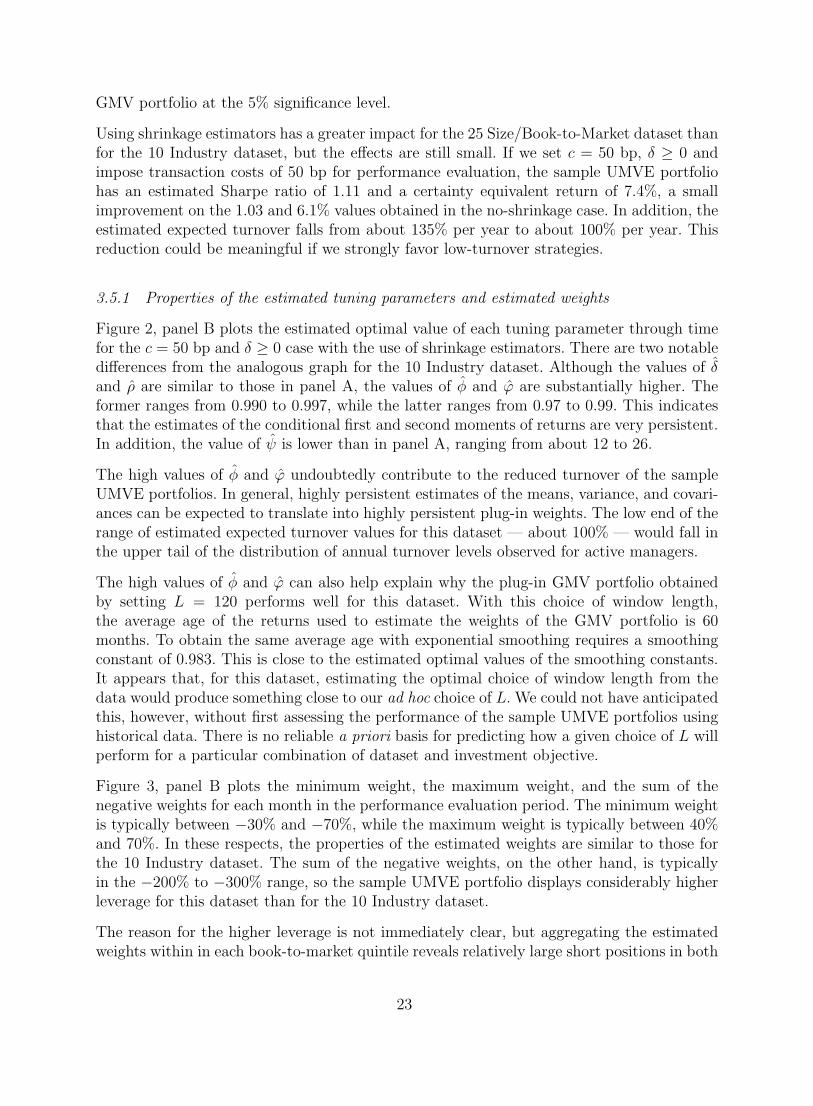
3.5.1 Properties of the estimated tuning parameters and estimated weights

Figure 2, panel B plots the estimated optimal value of each tuning parameter through timefor the c = 50 bp and δ ≥ 0 case with the use of shrinkage estimators. There are two notabledifferences from the analogous graph for the 10 Industry dataset. Although the values of δand ρ are similar to those in panel A, the values of φ and ϕ are substantially higher. Theformer ranges from 0.990 to 0.997, while the latter ranges from 0.97 to 0.99. This indicatesthat the estimates of the conditional first and second moments of returns are very persistent.In addition, the value of ψ is lower than in panel A, ranging from about 12 to 26.

The high values of φ and ϕ undoubtedly contribute to the reduced turnover of the sampleUMVE portfolios. In general, highly persistent estimates of the means, variance, and covari-ances can be expected to translate into highly persistent plug-in weights. The low end of therange of estimated expected turnover values for this dataset — about 100% — would fall inthe upper tail of the distribution of annual turnover levels observed for active managers.

The high values of φ and ϕ can also help explain why the plug-in GMV portfolio obtainedby setting L = 120 performs well for this dataset. With this choice of window length,the average age of the returns used to estimate the weights of the GMV portfolio is 60months. To obtain the same average age with exponential smoothing requires a smoothingconstant of 0.983. This is close to the estimated optimal values of the smoothing constants.It appears that, for this dataset, estimating the optimal choice of window length from thedata would produce something close to our ad hoc choice of L. We could not have anticipatedthis, however, without first assessing the performance of the sample UMVE portfolios usinghistorical data. There is no reliable a priori basis for predicting how a given choice of L willperform for a particular combination of dataset and investment objective.

Figure 3, panel B plots the minimum weight, the maximum weight, and the sum of thenegative weights for each month in the performance evaluation period. The minimum weightis typically between −30% and −70%, while the maximum weight is typically between 40%and 70%. In these respects, the properties of the estimated weights are similar to those forthe 10 Industry dataset. The sum of the negative weights, on the other hand, is typicallyin the −200% to −300% range, so the sample UMVE portfolio displays considerably higherleverage for this dataset than for the 10 Industry dataset.

The reason for the higher leverage is not immediately clear, but aggregating the estimatedweights within in each book-to-market quintile reveals relatively large short positions in both

23

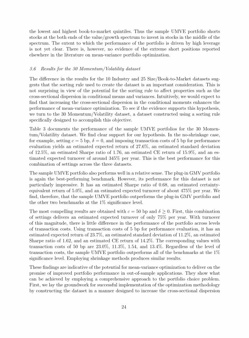
the lowest and highest book-to-market quintiles. Thus the sample UMVE portfolio shortsstocks at the both ends of the value/growth spectrum to invest in stocks in the middle of thespectrum. The extent to which the performance of the portfolio is driven by high leverageis not yet clear. There is, however, no evidence of the extreme short positions reportedelsewhere in the literature on mean-variance portfolio optimization.

3.6 Results for the 30 Momentum/Volatility dataset

The difference in the results for the 10 Industry and 25 Size/Book-to-Market datasets sug-gests that the sorting rule used to create the dataset is an important consideration. This isnot surprising in view of the potential for the sorting rule to affect properties such as thecross-sectional dispersion in conditional means and variances. Intuitively, we would expect tofind that increasing the cross-sectional dispersion in the conditional moments enhances theperformance of mean-variance optimization. To see if the evidence supports this hypothesis,we turn to the 30 Momentum/Volatility dataset, a dataset constructed using a sorting rulespecifically designed to accomplish this objective.

Table 3 documents the performance of the sample UMVE portfolios for the 30 Momen-tum/Volatility dataset. We find clear support for our hypothesis. In the no-shrinkage case,for example, setting c = 5 bp, δ = 0, and imposing transaction costs of 5 bp for performanceevaluation yields an estimated expected return of 27.6%, an estimated standard deviationof 12.5%, an estimated Sharpe ratio of 1.76, an estimated CE return of 15.9%, and an es-timated expected turnover of around 345% per year. This is the best performance for thiscombination of settings across the three datasets.

The sample UMVE portfolio also performs well in a relative sense. The plug-in GMV portfoliois again the best-performing benchmark. However, its performance for this dataset is notparticularly impressive. It has an estimated Sharpe ratio of 0.68, an estimated certainty-equivalent return of 5.0%, and an estimated expected turnover of about 475% per year. Wefind, therefore, that the sample UMVE portfolio outperforms the plug-in GMV portfolio andthe other two benchmarks at the 1% significance level.

The most compelling results are obtained with c = 50 bp and δ ≥ 0. First, this combinationof settings delivers an estimated expected turnover of only 75% per year. With turnoverof this magnitude, there is little difference in the performance of the portfolio across levelsof transaction costs. Using transaction costs of 5 bp for performance evaluation, it has anestimated expected return of 23.7%, an estimated standard deviation of 11.2%, an estimatedSharpe ratio of 1.62, and an estimated CE return of 14.2%. The corresponding values withtransaction costs of 50 bp are 23.0%, 11.3%, 1.54, and 13.4%. Regardless of the level oftransaction costs, the sample UMVE portfolio outperforms all of the benchmarks at the 1%significance level. Employing shrinkage methods produces similar results.

These findings are indicative of the potential for mean-variance optimization to deliver on thepromise of improved portfolio performance in out-of-sample applications. They show whatcan be achieved by employing a comprehensive approach to the portfolio choice problem.First, we lay the groundwork for successful implementation of the optimization methodologyby constructing the dataset in a manner designed to increase the cross-sectional dispersion

24

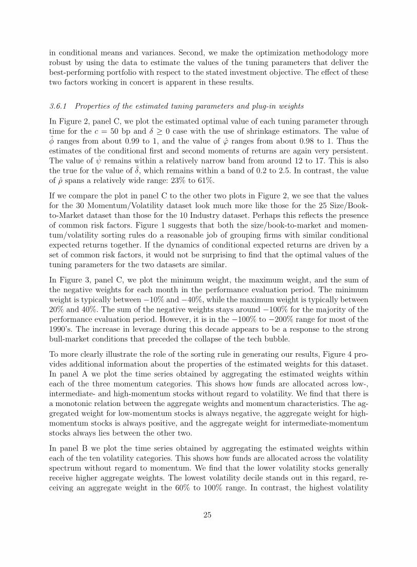
in conditional means and variances. Second, we make the optimization methodology morerobust by using the data to estimate the values of the tuning parameters that deliver thebest-performing portfolio with respect to the stated investment objective. The effect of thesetwo factors working in concert is apparent in these results.

3.6.1 Properties of the estimated tuning parameters and plug-in weights

In Figure 2, panel C, we plot the estimated optimal value of each tuning parameter throughtime for the c = 50 bp and δ ≥ 0 case with the use of shrinkage estimators. The value ofφ ranges from about 0.99 to 1, and the value of ϕ ranges from about 0.98 to 1. Thus theestimates of the conditional first and second moments of returns are again very persistent.The value of ψ remains within a relatively narrow band from around 12 to 17. This is alsothe true for the value of δ, which remains within a band of 0.2 to 2.5. In contrast, the valueof ρ spans a relatively wide range: 23% to 61%.

If we compare the plot in panel C to the other two plots in Figure 2, we see that the valuesfor the 30 Momentum/Volatility dataset look much more like those for the 25 Size/Book-to-Market dataset than those for the 10 Industry dataset. Perhaps this reflects the presenceof common risk factors. Figure 1 suggests that both the size/book-to-market and momen-tum/volatility sorting rules do a reasonable job of grouping firms with similar conditionalexpected returns together. If the dynamics of conditional expected returns are driven by aset of common risk factors, it would not be surprising to find that the optimal values of thetuning parameters for the two datasets are similar.

In Figure 3, panel C, we plot the minimum weight, the maximum weight, and the sum ofthe negative weights for each month in the performance evaluation period. The minimumweight is typically between −10% and −40%, while the maximum weight is typically between20% and 40%. The sum of the negative weights stays around −100% for the majority of theperformance evaluation period. However, it is in the −100% to −200% range for most of the1990’s. The increase in leverage during this decade appears to be a response to the strongbull-market conditions that preceded the collapse of the tech bubble.

To more clearly illustrate the role of the sorting rule in generating our results, Figure 4 pro-vides additional information about the properties of the estimated weights for this dataset.In panel A we plot the time series obtained by aggregating the estimated weights withineach of the three momentum categories. This shows how funds are allocated across low-,intermediate- and high-momentum stocks without regard to volatility. We find that there isa monotonic relation between the aggregate weights and momentum characteristics. The ag-gregated weight for low-momentum stocks is always negative, the aggregate weight for high-momentum stocks is always positive, and the aggregate weight for intermediate-momentumstocks always lies between the other two.

In panel B we plot the time series obtained by aggregating the estimated weights withineach of the ten volatility categories. This shows how funds are allocated across the volatilityspectrum without regard to momentum. We find that the lower volatility stocks generallyreceive higher aggregate weights. The lowest volatility decile stands out in this regard, re-ceiving an aggregate weight in the 60% to 100% range. In contrast, the highest volatility

25

deciles typically receive a weight close to zero. The exception to this is during the 1990swhen an increasing long position in the most volatile decile is balanced against an increasingshort position in decile nine. These results suggest that the sorting rule plays a significantrole in determining the performance of the sample UMVE portfolios for this dataset.

3.7 Incorporating short-sales constraints

A potential criticism of the results presented in Tables 1–3 is that all investors face somelimits on selling securities short. We can address this criticism by modifying the frameworkdeveloped in Section 2 to include weight constraints. To illustrate, suppose that short salesare prohibited. If we take the values of ψ, φ, and ϕ as given, we can use numerical methodsto solve the quadratic program

maxwt

w′tµt(φ)− ψ

2w′

tΩt(ϕ)wt,

s.t. w′tι = 1,

wit ≥ 0, i = 1, 2, . . . , N,

(37)

for any period t. The solution to this program is the vector of plug-in weights for periodt under the long-only constraint. Accordingly, we construct the long-only version of thesample objective function for period T0 by using these weights in place of the Ferson andSiegel (2001) weights for t = K0, K0 + 1, . . . , T0, and proceed in an analogous fashion foreach subsequent period. In all other respects, the analysis goes through unchanged. A similarapproach can be used to accommodate more general weight constraints.

Table 4 summarizes the results obtained for each dataset under a long-only constraint for theshrinkage-estimators case. We begin with the results in panel A for the 10 Industry dataset.Prohibiting short sales clearly has a meaningful impact on the performance of the sampleUMVE portfolios. For example, setting c = 50 bp, δ ≥ 0, and assuming transaction costs of 50bp for performance evaluation yields an estimated Sharpe ratio of 0.79 and an estimated CEreturn of 2.7%, substantially lower than the corresponding values of 1.04 and 5.2% reportedin Table 1. Nonetheless, the long-only sample UMVE portfolio still outperforms the S&P 500index and naıve diversification at the 1% significance level and the long-only GMV portfolioat the 10% significance level. Thus the leverage generated by short sales does not appear tobe an overriding factor in determining the performance of mean-variance optimization forthis dataset.

The results in panel B show that prohibiting short sales has a larger effect on portfolioperformance for the 25 Size/Book-to-Market dataset. For example, setting c = 50 bp, δ ≥ 0,and assuming transaction costs of 50 bp for performance evaluation yields an estimatedSharpe ratio of 0.64 and an estimated CE return of −3.5%, as opposed to the values of1.11 and 7.4% reported in Table 2. Although the estimated Sharpe ratio of the long-onlysample UMVE portfolio is higher than that of any of the benchmarks, it is not high enoughto conclude that the performance advantage is statistically significant. We noted earlier thatthe unconstrained portfolios display considerably higher leverage for the 25 Size/Book-to-Market dataset than for the 10 Industry dataset. The evidence in Table 4 suggests that high

26

leverage is a key contributor to the performance of the portfolio in the unconstrained casefor this dataset.

In terms of methodology, the results in panel C for the 30 Momentum/Volatility datasetare the most interesting. Setting c = 50 bp, δ ≥ 0, and assuming transaction costs of 50bp for performance evaluation yields an estimated Sharpe ratio of 1.04 and an estimatedCE return of 8.7%. The values of 1.64 and 14.3% reported in Table 3 are of course moreimpressive, but it is noteworthy that the long-only sample UMVE portfolio outperforms allof the benchmarks at the 1% significance level, and it does so with an estimated expectedturnover of less than 10% per year. This supports our contention that expanding the scopeof the optimization problem to include the sorting scheme enhances portfolio performance.

We should also point out that in no instance does imposing the long-only constraint leadto an increase in the estimated Sharpe ratio of the portfolio. It seems obvious that weshould expect this to be the case. However, some studies in the literature report the oppositefinding (e.g., see Table 3 of DeMiguel et al., 2009). This again raises questions about theefficacy of the research designed used in these studies. It would be surprising to find thatimposing additional constraints on the portfolio improves its performance when using arobust approach for exploiting sample information.

3.8 Reward and risk analysis using factor models

The analysis thus far has examined the performance of the sample UMVE portfolios relativeto a number of common benchmarks. To develop a more complete picture of the performancelandscape, we use a linear factor model to analyze the reward and risk characteristics of theportfolios. Specifically, we fit the Carhart (1997) extension of the Fama and French (1993)three-factor model to the excess returns on the sample UMVE portfolios. The Carhart (1997)model includes market, size, book-to-market, and momentum factors. 19 In the interest ofspace, we focus on the case using shrinkage estimators, with c = 50 bp, δ ≥ 0, and assumingtransaction costs of 50 bp for performance evaluation.

Table 5 summarizes the results of the factor model regressions. We begin with panel A, whichpresents results for the scenario with unconstrained weights. The estimated annualized alphasof the sample UMVE portfolios range from 4.6% for the 10 Industry dataset to 11.2% forthe 30 Volatility/Momentum dataset; all of the estimates are statistically significant. Hence,the evidence indicates that the average returns for the sample UMVE portfolios contain acomponent that is not captured by this model. This finding is not surprising. In general,we would not expect an unconditional factor model to fully explain the average returns forthe sample UMVE portfolios because these portfolios have time-varying weights and hencetime-varying expected returns.

The estimated factor loadings and R2 values for the three datasets are more interesting. Allof the estimated loadings for the 10 Industry dataset are positive and statistically signifi-cant. However, the largest is only 0.6, indicating that the sample UMVE portfolio returns

19 The monthly factor returns and one-month T-bill rate are obtained from the Ken French datalibrary (http://mba.tuck.dartmouth.edu/pages/faculty/ken.french/data library.html).

27

for this dataset are relatively insensitive to these sources of systematic risk. In addition, theR2 for the regression is only 62%, so a substantial portion of the risk of the portfolio isidiosyncratic. Like the estimated alphas, this is consistent with the presence of time-varyingfactor exposures that cannot be captured using an unconditional factor model. The regres-sions for the 25 Size/Book-to-Market and 30 Volatility/Momentum datasets also producerelatively low R2 values: 65% and 59%. But not all of the estimated factor loadings arestatistically significant. The sample UMVE portfolio for the 25 Size/Book-to-Market has nostatistically significant exposure to the size and momentum factors, and the portfolio for the30 Volatility/Momentum dataset has no statistically significant exposure to the size factor.

Panel B shows how the results change under the long-only constraint. First, the estimatedalphas decrease to 1.7% for the 10 Industry and the 25 Size/Book-to-Market datasets and to3.7% for the 30 Volatility/Momentum dataset. Imposing the constraint reduces the magni-tude of the unexplained component of the average portfolio returns. Second, the regression R2

increases to 78% for the 10 Industry and 30 Volatility/Momentum datasets, and to 92% forthe 25 Size/Book-to-Market. Imposing the constraint reduces the idiosyncratic componentof risk. Third, all of the estimated factor loadings are statistically significant.

3.9 Additional robustness checks

Before concluding we discuss two additional robustness checks to address potential concernsabout our research design. First, we determine if our findings are overly sensitive to the valueof γ used to construct the sample objective function. Although our choice of γ will clearlyaffect the aggressiveness of the sample UMVE portfolios, we want to exclude the possibilitythat this alters the overall conclusions about the performance of our methodology. To do so,we repeat the empirical analysis using γ = 5 instead of γ = 15. As expected, the results areindicative of a much more aggressive investment style. For example, if we set c = 50 bp, δ ≥ 0,assume transaction costs of 50 bp for performance evaluation, and use shrinkage estimators ofthe conditional moments of returns, the sample UMVE portfolio for the 10 Industry datasethas an estimated expected return of 38.8%, an estimated standard deviation of 27.1%, anestimated Sharpe ratio of 1.23, an estimated CE return of 20.4%, and an estimated expectedturnover of 818% per year. But changing the value of γ does not affect our general conclusionsregarding the performance of the sample UMVE portfolio. It still outperforms all three ofthe benchmarks at the 1% significance level.

Second, we determine whether using equally-weighted portfolios as assets has a undue in-fluence on the results. Perhaps this explains why our methodology performs so well in com-parison to the methodologies employed in prior studies that use value-weighted portfoliosas assets. To exclude this possibility, we repeat the empirical analysis for versions of the 10Industry and 25 Size/Book-to-Market datasets that contain value-weighted portfolios. Thisdoes produce some changes in the results. For instance, both the estimated Sharpe ratiosand estimated expected turnover figures for the 10 Industry dataset are lower than those re-ported in Table 1. But the performance comparisons remain favorable to the sample UMVEportfolios. For example, if we use shrinkage estimators, set c = 50 bp, δ ≥ 0, and assumetransaction costs of 50 bp for performance evaluation, the sample UMVE portfolio for the25 Size/BTM dataset has an estimated expected return of 17%, an estimated standard de-

28

viation of 13%, an estimated Sharpe ratio of 0.89, an estimated CE return of 4.6%, andan estimated expected turnover of 84% per year. This is sufficient to outperform all threebenchmarks at the 5% level. Thus the choice of weighting scheme does not seem to be acritical issue.

4 Closing Remarks

Mean-variance portfolio optimization has recently come under fire for its ostensibly poorperformance in out-of-sample applications. Much of this recent criticism is motivated byDeMiguel et al. (2009). The authors of this study construct sample mean-variance efficientportfolios using several variants of the plug-in approach and find that naıve diversificationoutperforms these portfolios for most of the datasets considered. This poor showing by thesample mean-variance efficient portfolios, which is interpreted as evidence that “the errorsin estimating means and covariances erode all the gains from optimal, relative to naive,diversification,” leads the authors to conclude that “there are still many ‘miles to go’ beforethe gains promised by optimal portfolio choice can actually be realized out of sample.”

Our investigation supports a sharply contrasting view of the out-of-sample performance ofmean-variance optimization. We begin by noting that many aspects of the plug-in approach,such as how to model changes in the investment opportunity set and how to estimate themodel parameters, fall outside the scope of the traditional optimization framework. Thisgives rise to significant robustness issues because ad hoc choices with respect to the details ofthe research design can lead to unforeseen consequences. For example, DeMiguel et al. (2009)focus on the performance of the sample version of the tangency portfolio, which is obtainedby implementing the plug-in approach using a time-varying value of relative risk aversion.Although in principle this is fine, it leads to extreme turnover and poor performance becausethe sample tangency portfolio frequently targets a conditional expected return in excess of100% per year (Kirby and Ostdiek, 2012).

To address the optimization problem in a more comprehensive fashion, we expand the scope ofthe analysis to encompass the effects of estimation risk, specification errors, and transactioncosts on portfolio performance, and we use an adaptive empirical procedure to select thevalues of the unknown parameters that appear in the expression for the plug-in weights. Theempirical analysis demonstrates that our methodology leads to robust portfolio selectionrules, regardless of whether transaction costs are high or low. The resulting sample UMVEportfolios have well-behaved weights, reasonable turnover, and substantially higher estimatedSharpe ratios and certainty-equivalent returns than common performance benchmarks suchas the 1/N portfolio and S&P 500 index. This is true regardless of whether we permit shortsales or impose a long-only constraint.

As further evidence on the value of taking a comprehensive approach to the optimizationproblem, we show that constructing the dataset by sorting firms into portfolios on the basis ofhistorical measures of momentum and volatility leads to sample UMVE portfolios that per-form particularly well. Indeed, the sample UMVE portfolios for the 30 Momentum/Volatilitydataset outperform the S&P 500 index, 1/N portfolio, and a simple plug-in version of theGMV portfolio at the 1% significance level. This finding is noteworthy because prior studies

29

report that the GMV portfolio performs well relative to other sample efficient portfolios.In view of this finding and the evidence in general, we believe the proposed methodologyrepresents a significant step forward in addressing the challenges of mean-variance portfoliochoice in the presence of estimation risk, model misspecification, and transaction costs.

With respect to future research, there are a number of interesting ways to extend the method-ology. One possibility is to expand the information set by allowing the conditional momentsof returns to depend on both past returns and other financial variables, such as interest rates,dividend yields and credit spreads. Another is to further expand the scope of the optimiza-tion problem by allowing the number of portfolios N under a given sorting rule to be anadditional tuning parameter. This would allow the data to inform our choice of the scale ofthe optimization problem rather than imposing the scale a priori. We are currently pursingideas along these lines.

30

References

Brandt, M., P. Santa-Clara, and R. Valkanov, 2009, Parametric portfolio policies: Exploitingcharacteristics in the cross-section of equity returns, Review of Financial Studies 22, 3411–3447

Carhart, M., 1997, On persistence in mutual fund performance, Journal of Finance 52, 57–82.

Chan, L., J. Karceski, and J. Lakonishok, 1999, On portfolio optimization: Forecasting co-variances and choosing the risk model, Review of Financial Studies 12, 937–974.

DeMiguel, V., L. Garlappi, and R. Uppal, 2009, Optimal versus naive diversification: Howinefficient is the 1/N portfolio strategy, Review of Financial Studies 22, 1915–1953.

Domowitz, I., J. Glen, and A. Madhavan, 2001, Liquidity, volatility, and equity trading costsacross countries and over time, International Finance 4, 221–255.

Dybvig, P., and S. Ross, 1985, Differential information and performance measurement usinga security market line, Journal of Finance 40, 383–399.

Fama, E., and K. French, 1993, Common risk factors in the returns on stocks and bonds,Journal of Financial Economics 33, 3–56.

Ferson, W., and A. Siegel, 2001, The efficient use of conditioning information in portfolios,Journal of Finance 56, 967–982.

Foster, D, and D. Nelson, 1996, Continuous record asymptotics for rolling sample varianceestimators, Econometrica 64, 139–174.

Griffin, J., and J. Xu, 2007, How Smart are the Smart Guys? A Unique View from HedgeFund Stock Holdings, Review of Financial Studies 22, 2531–2570.

Hansen, L., 1982, Large sample properties of generalized method of moments estimators,Econometrica 50, 1029–1054.

Hansen, L., and S. Richard, 1987, The role of conditioning information in deducing testablerestrictions implied by dynamic asset pricing models, Econometrica 55, 587– 613.

Hasbrouck, J., 2009, Trading costs and returns for US equities: Estimating effective costsfrom daily data, Journal of Finance 64, 1445–1477.

Jagannathan, R., and T. Ma., 2003, Risk reduction in large portfolios: Why imposing thewrong constraints helps, Journal of Finance 58, 1651–1684.

James, W., and C. Stein, 1961, Estimation with quadratic loss, Proceedings of the FourthBerkeley Symposium on Mathematics and Statistics, 361–379.

Kan, R., and G. Zhou, 2007, Optimal portfolio choice with parameter uncertainty, Journalof Financial and Quantitative Analysis 42, 621–656.

Kirby, C., and B. Ostdiek, 2012, It’s all in the timing: Simple active portfolio strategiesthat outperform naıve diversification, Journal of Financial and Quantitative Analysis 47,437–467

Ledoit, O., and M. Wolf, 2004, Honey, I shrunk the sample covariance matrix: Problems inmean-variance optimization, Journal of Portfolio Management 30, 110–119.

31

Leland, H., 1999, Optimal portfolio management with transactions costs and capital gainstaxes, working paper, University of California Berkeley.

Merton, R., 1980, On estimating the expected return on the market: An exploratory inves-tigation, Journal of Financial Economics 8, 323–361.

Patton, A., and A. Timmermann, 2007, Properties of optimal forecasts under asymmetricloss and nonlinearity, Journal of Econometrics 140, 884–918.

Paye, B., 2010, Portfolios of estimated portfolios: Combination approaches to estimatingoptimal portfolio weights, working paper, University of Georgia.

Skouras, S., 2007. Decisionmetrics: A decision-based approach to econometric modelling,Journal of Econometrics 137, 414-440.

Tu, J., and G. Zhou, 2011, Markowitz meets Talmud: A combination of sophisticated andnaive diversification strategies, Journal of Financial Economics 99, 204–215.

32

Table

1Perf

orm

ance

ofSam

ple

UM

VE

Port

folios

for

the

10

Indust

ryD

ata

set

The

tabl

edo

cum

ents

the

perf

orm

ance

ofth

esa

mpl

eU

MV

Epo

rtfo

lios

for

the

10In

dust

ryda

tase

t.R

esul

tsfo

rth

eth

ree

benc

hmar

ks(S

&P

500,

1/N

,an

dpl

ug-in

GM

Vpo

rtfo

lios)

are

pres

ente

dab

ove

pane

lA

.Fo

rea

chpo

rtfo

lio,

we

repo

rtan

nual

ized

esti

mat

esof

the

expe

cted

turn

over

(τp),

the

expe

cted

retu

rn(µ

p),

retu

rnvo

lati

lity

(σp),

Shar

pera

tio

(λp),

and

cert

aint

y-eq

uiva

lent

retu

rn(Q

p).

The

p-v

alue

sin

dica

teth

epr

obab

ility

ofob

tain

ing

ahi

gher

λp

unde

rth

enu

llhy

poth

esis

that

the

corr

espo

ndin

gbe

nchm

ark

port

folio

perf

orm

sat

leas

tas

wel

las

the

UM

VE

port

folio

.T

hesa

mpl

eU

MV

Epo

rtfo

lios

are

cons

truc

ted

usin

ga

rela

tive

risk

aver

sion

ofγ

=15

wit

hex

pone

ntia

lsm

ooth

ing

esti

mat

ors

ofth

eco

ndit

iona

lm

ean

vect

oran

dco

ndit

iona

lse

cond

-mom

ent

mat

rix.

All

para

met

ers

inth

eex

pres

sion

for

the

opti

mal

port

folio

wei

ghts

are

esti

mat

edus

ing

anap

proa

chde

sign

edto

min

imiz

eth

ead

vers

eim

pact

ofes

tim

atio

nri

skan

dre

bala

ncin

gco

sts

asde

scri

bed

inth

ete

xt.

The

anal

ysis

isco

nduc

ted

wit

hbo

thfu

ll-an

dpa

rtia

l-ad

just

men

tof

the

port

folio

wei

ghts

(δ=

0an

dδ≥

0)us

ing

two

leve

lsof

prop

orti

onal

tran

sact

ion

cost

sto

cons

truc

tth

esa

mpl

eob

ject

ive

func

tion

(c=

5an

dc

=50

basi

spo

ints

).Fo

rea

chva

lue

ofc,

we

repo

rtµ

p,

σp,

λp,

and

Qp

usin

gre

turn

sm

easu

red

net

ofpr

opor

tion

alon

e-w

aytr

ansa

ctio

nco

sts

ofbo

thfiv

ean

d50

basi

spo

ints

.T

hepe

rfor

man

ceev

alua

tion

peri

odis

Janu

ary

1976

toD

ecem

ber

2009

(408

mon

ths)

.

Impos

ing

Tra

nsa

ctio

nC

osts

of5

bp

Impos

ing

Tra

nsa

ctio

nC

osts

of50

bp

pvs

.p

vs.

pvs

.p

vs.

pvs

.p

vs.

τ pµ

pσ

pλ

pQ

pM

kt1/

NG

MV

µp

σp

λp

Qp

Mkt

1/N

GM

V

S&P

500

011

.84

15.2

70.

41-5

.65

−0.

879

0.54

311

.84

15.2

70.

41-5

.65

−0.

868

0.32

91/

N14

16.2

619

.46

0.55

-12.

150.

121

−0.

299

16.1

419

.46

0.54

-12.

260.

132

−0.

162

GM

V13

810

.63

11.8

30.

430.

130.

457

0.70

1−

9.39

11.8

70.

33-1

.18

0.67

10.

838

−

Pan

elA

:N

oShri

nka

ge

c=

5bp

,δ

=0

1424

33.2

716

.80

1.65

12.0

90.

000

0.00

00.

000

20.1

917

.33

0.85

-2.3

20.

014

0.08

50.

002

c=

5bp

,δ≥

014

2433

.27

16.8

01.

6512

.09

0.00

00.

000

0.00

020

.19

17.3

30.

85-2

.32

0.01

40.

085

0.00

2c

=50

bp,δ

=0

381

21.6

113

.36

1.21

8.23

0.00

00.

000

0.00

018

.14

13.4

70.

944.

530.

001

0.02

20.

000

c=

50bp

,δ≥

033

621

.96

13.8

41.

197.

600.

000

0.00

00.

000

18.9

013

.95

0.96

4.32

0.00

10.

016

0.00

0

Pan

elB

:U

sing

Shri

nka

geEst

imat

ors

c=

5bp

,δ

=0

1381

36.5

017

.91

1.73

12.4

30.

000

0.00

00.

000

23.8

218

.61

0.98

-2.1

50.

003

0.02

10.

000

c=

5bp

,δ≥

013

8136

.50

17.9

11.

7312

.43

0.00

00.

000

0.00

023

.82

18.6

10.

98-2

.15

0.00

30.

021

0.00

0c

=50

bp,δ

=0

326

22.9

713

.70

1.28

8.90

0.00

00.

000

0.00

020

.02

13.8

71.

055.

590.

000

0.00

20.

000

c=

50bp

,δ≥

028

622

.73

13.9

31.

248.

180.

000

0.00

00.

000

20.1

414

.13

1.04

5.18

0.00

00.

003

0.00

0

Table

2Perf

orm

ance

ofSam

ple

UM

VE

Port

folios

for

the

25

Siz

e/B

ook-t

o-M

ark

et

Data

set

The

tabl

edo

cum

ents

the

perf

orm

ance

ofth

esa

mpl

eU

MV

Epo

rtfo

lios

for

the

25Si

ze/B

ook-

to-M

arke

tda

tase

t.R

esul

tsfo

rth

eth

ree

benc

hmar

ks(S

&P

500,

1/N

,and

plug

-in

GM

Vpo

rtfo

lios)

are

pres

ente

dab

ove

pane

lA.F

orea

chpo

rtfo

lio,w

ere

port

annu

aliz

edes

tim

ates

ofth

eex

pect

edtu

rnov

er(τ

p),

the

expe

cted

retu

rn(µ

p),

retu

rnvo

lati

lity

(σp),

Shar

pera

tio

(λp),

and

cert

aint

y-eq

uiva

lent

retu

rn(Q

p).

The

p-v

alue

sin

dica

teth

epr

obab

ility

ofob

tain

ing

ahi

gher

λp

unde

rth

enu

llhy

poth

esis

that

the

corr

espo

ndin

gbe

nchm

ark

port

folio

perf

orm

sat

leas

tas

wel

las

the

UM

VE

port

folio

.T

hesa

mpl

eU

MV

Epo

rtfo

lios

are

cons

truc

ted

usin

ga

rela

tive

risk

aver

sion

ofγ

=15

wit

hex

pone

ntia

lsm

ooth

ing

esti

mat

ors

ofth

eco

ndit

iona

lm

ean

vect

oran

dco

ndit

iona

lse

cond

-mom

ent

mat

rix.

All

para

met

ers

inth

eex

pres

sion

for

the

opti

mal

port

folio

wei

ghts

are

esti

mat

edus

ing

anap

proa

chde

sign

edto

min

imiz

eth

ead

vers

eim

pact

ofes

tim

atio

nri

skan

dre

bala

ncin

gco

sts

asde

scri

bed

inth

ete

xt.

The

anal

ysis

isco

nduc

ted

wit

hbo

thfu

ll-an

dpa

rtia

l-ad

just

men

tof

the

port

folio

wei

ghts

(δ=

0an

dδ≥

0)us

ing

two

leve

lsof

prop

orti

onal

tran

sact

ion

cost

sto

cons

truc

tth

esa

mpl

eob

ject

ive

func

tion

(c=

5an

dc

=50

basi

spo

ints

).Fo

rea

chva

lue

ofc,

we

repo

rtµ

p,

σp,

λp,

and

Qp

usin

gre

turn

sm

easu

red

net

ofpr

opor

tion

alon

e-w

aytr

ansa

ctio

nco

sts

ofbo

thfiv

ean

d50

basi

spo

ints

.T

hepe

rfor

man

ceev

alua

tion

peri

odis

Janu

ary

1976

toD

ecem

ber

2009

(408

mon

ths)

.

Impos

ing

Tra

nsa

ctio

nC

osts

of5

bp

Impos

ing

Tra

nsa

ctio

nC

osts

of50

bp

pvs

.p

vs.

pvs

.p

vs.

pvs

.p

vs.

τ pµ

pσ

pλ

pQ

pM

kt1/

NG

MV

µp

σp

λp

Qp

Mkt

1/N

GM

V

S&P

500

011

.84

15.2

70.

41-5

.65

−0.

956

1.00

011

.84

15.2

70.

41-5

.65

−0.

950

0.99

61/

N11

15.8

318

.00

0.57

-8.4

70.

044

−1.

000

15.7

318

.00

0.57

-8.5

70.

050

−0.

956

GM

V49

521

.22

12.8

51.

228.

840.

000

0.00

0−

16.7

012

.90

0.86

4.21

0.00

40.

044

−

Pan

elA

:N

oShri

nka

ge

c=

5bp

,δ

=0

464

21.9

312

.61

1.30

10.0

10.

000

0.00

00.

150

17.7

212

.84

0.95

5.35

0.00

10.

017

0.13

1c

=5

bp,δ≥

045

921

.92

12.6

21.

299.

980.

000

0.00

00.

157

17.7

512

.85

0.95

5.36

0.00

10.

017

0.12

7c

=50

bp,δ

=0

286

19.9

012

.36

1.16

8.44

0.00

00.

000

0.79

417

.30

12.4

30.

955.

710.

000

0.00

80.

134

c=

50bp

,δ≥

013

720

.47

13.0

81.

147.

640.

000

0.00

00.

833

19.2

413

.26

1.03

6.05

0.00

00.

003

0.02

7

Pan

elB

:U

sing

Shri

nka

geEst

imat

ors

c=

5bp

,δ

=0

372

22.6

812

.69

1.34

10.6

10.

000

0.00

00.

101

19.3

313

.10

1.05

6.45

0.00

00.

003

0.03

4c

=5

bp,δ≥

037

022

.66

12.6

91.

3410

.59

0.00

00.

000

0.10

419

.33

13.1

11.

056.

440.

000

0.00

30.

033

c=

50bp

,δ

=0

176

21.0

712

.60

1.23

9.15

0.00

00.

000

0.47

419

.47

12.7

31.

097.

320.

000

0.00

10.

018

c=

50bp

,δ≥

099

20.8

212

.77

1.19

8.59

0.00

00.

000

0.60

819

.93

12.9

11.

117.

430.

000

0.00

10.

013

Table

3Perf

orm

ance

ofSam

ple

UM

VE

Port

folios

for

the

30

Mom

entu

m/V

ola

tility

Data

set

The

tabl

edo

cum

ents

the

perf

orm

ance

ofth

esa

mpl

eU

MV

Epo

rtfo

lios

for

the

30M

omen

tum

/Vol

atili

tyda

tase

t.R

esul

tsfo

rth

eth

ree

benc

hmar

ks(S

&P

500,

1/N

,and

plug

-in

GM

Vpo

rtfo

lios)

are

pres

ente

dab

ove

pane

lA.F

orea

chpo

rtfo

lio,w

ere

port

annu

aliz

edes

tim

ates

ofth

eex

pect

edtu

rnov

er(τ

p),

the

expe

cted

retu

rn(µ

p),

retu

rnvo

lati

lity

(σp),

Shar

pera

tio

(λp),

and

cert

aint

y-eq

uiva

lent

retu

rn(Q

p).

The

p-v

alue

sin

dica

teth

epr

obab

ility

ofob

tain

ing

ahi

gher

λp

unde

rth

enu

llhy

poth

esis

that

the

corr

espo

ndin

gbe

nchm

ark

port

folio

perf

orm

sat

leas

tas

wel

las

the

UM

VE

port

folio

.T

hesa

mpl

eU

MV

Epo

rtfo

lios

are

cons

truc

ted

usin

ga

rela

tive

risk

aver

sion

ofγ

=15

wit

hex

pone

ntia

lsm

ooth

ing

esti

mat

ors

ofth

eco

ndit

iona

lm

ean

vect

oran

dco

ndit

iona

lse

cond

-mom

ent

mat

rix.

All

para

met

ers

inth

eex

pres

sion

for

the

opti

mal

port

folio

wei

ghts

are

esti

mat

edus

ing

anap

proa

chde

sign

edto

min

imiz

eth

ead

vers

eim

pact

ofes

tim

atio

nri

skan

dre

bala

ncin

gco

sts

asde

scri

bed

inth

ete

xt.

The

anal

ysis

isco

nduc

ted

wit

hbo

thfu

ll-an

dpa

rtia

l-ad

just

men

tof

the

port

folio

wei

ghts

(δ=

0an

dδ≥

0)us

ing

two

leve

lsof

prop

orti

onal

tran

sact

ion

cost

sto

cons

truc

tth

esa

mpl

eob

ject

ive

func

tion

(c=

5an

dc

=50

basi

spo

ints

).Fo

rea

chva

lue

ofc,

we

repo

rtµ

p,

σp,

λp,

and

Qp

usin

gre

turn

sm

easu

red

net

ofpr

opor

tion

alon

e-w

aytr

ansa

ctio

nco

sts

ofbo

thfiv

ean

d50

basi

spo

ints

.T

hepe

rfor

man

ceev

alua

tion

peri

odis

Janu

ary

1976

toD

ecem

ber

2009

(408

mon

ths)

.

Impos

ing

Tra

nsa

ctio

nC

osts

of5

bp

Impos

ing

Tra

nsa

ctio

nC

osts

of50

bp

pvs

.p

vs.

pvs

.p

vs.

pvs

.p

vs.

τ pµ

pσ

pλ

pQ

pM

kt1/

NG

MV

µp

σp

λp

Qp

Mkt

1/N

GM

V

S&P

500

011

.84

15.2

70.

41-5

.65

−0.

905

0.84

011

.84

15.2

70.

41-5

.65

−0.

896

0.23

21/

N14

16.8

519

.88

0.57

-12.

790.

095

−0.

658

16.7

319

.88

0.56

-12.

900.

104

−0.

096

GM

V47

612

.05

9.67

0.68

5.04

0.16

00.

342

−7.

759.

850.

230.

480.

768

0.90

4−

Pan

elA

:N

oShri

nka

ge

c=

5bp

,δ

=0

344

27.5

712

.49

1.76

15.8

70.

000

0.00

00.

000

24.4

512

.78

1.48

12.2

10.

000

0.00

10.

000

c=

5bp

,δ≥

034

427

.57

12.4

91.

7615

.87

0.00

00.

000

0.00

024

.45

12.7

81.

4812

.21

0.00

00.

001

0.00

0c

=50

bp,δ

=0

158

22.0

610

.20

1.62

14.2

50.

000

0.00

00.

000

20.6

410

.38

1.46

12.5

60.

000

0.00

10.

000

c=

50bp

,δ≥

075

23.6

811

.22

1.62

14.2

40.

000

0.00

00.

000

23.0

111

.31

1.54

13.4

20.

000

0.00

00.

000

Pan

elB

:U

sing

Shri

nka

geEst

imat

ors

c=

5bp

,δ

=0

230

28.5

813

.54

1.71

14.8

40.

000

0.00

00.

000

26.5

113

.78

1.53

12.2

60.

000

0.00

00.

000

c=

5bp

,δ≥

023

028

.58

13.5

41.

7014

.84

0.00

00.

000

0.00

026

.51

13.7

81.

5312

.26

0.00

00.

000

0.00

0c

=50

bp,δ

=0

110

24.8

111

.90

1.63

14.1

80.

000

0.00

00.

000

23.8

112

.02

1.53

12.9

80.

000

0.00

00.

000

c=

50bp

,δ≥

069

25.9

412

.44

1.64

14.3

30.

000

0.00

00.

000

25.3

312

.55

1.58

13.5

20.

000

0.00

00.

000

Table

4Perf

orm

ance

ofSam

ple

UM

VE

Port

folios

under

aLong-O

nly

Const

rain

tT

heta

ble

docu

men

tsth

epe

rfor

man

ceof

sam

ple

long

-onl

yU

MV

Epo

rtfo

lios

usin

ga

rela

tive

risk

aver

sion

ofγ

=15

and

shri

nkag

ees

tim

ator

s.Fo

rea

chpo

rtfo

lio,w

ere

port

annu

aliz

edes

tim

ates

ofth

eex

pect

edtu

rnov

er(τ

p),

the

expe

cted

retu

rn(µ

p),

retu

rnvo

lati

lity

(σp),

Shar

pera

tio

(λp),

and

cert

aint

y-eq

uiva

lent

retu

rn(Q

p).

The

p-v

alue

sin

dica

teth

epr

obab

ility

ofob

tain

ing

ahi

gher

λp

unde

rth

enu

llhy

poth

esis

that

the

corr

espo

ndin

gbe

nchm

ark

port

folio

(S&

P50

0,1/

N,

orpl

ug-in

long

-onl

yG

MV

)pe

rfor

ms

atle

ast

asw

ell

asth

eU

MV

Epo

rtfo

lio.

The

sam

ple

UM

VE

port

folio

sar

eco

nstr

ucte

dus

ing

expo

nent

ial

smoo

thin

ges

tim

ator

sof

the

cond

itio

nal

mea

nve

ctor

and

cond

itio

nal

seco

nd-m

omen

tm

atri

x.A

llpa

ram

eter

sin

the

expr

essi

onfo

rth

eop

tim

alpo

rtfo

liow

eigh

tsar

ees

tim

ated

usin

gan

appr

oach

desi

gned

tom

inim

ize

the

adve

rse

impa

ctof

esti

mat

ion

risk

and

reba

lanc

ing

cost

sas

desc

ribe

din

the

text

.T

hean

alys

isis

cond

ucte

dw

ith

both

full-

and

part

ial-ad

just

men

tof

the

port

folio

wei

ghts

(δ=

0an

dδ≥

0)us

ing

two

leve

lsof

prop

orti

onal

tran

sact

ion

cost

sto

cons

truc

tth

esa

mpl

eob

ject

ive

func

tion

(c=

5an

dc

=50

basi

spo

ints

).Fo

rea

chva

lue

ofc,

we

repo

rtµ

p,σ

p,λ

p,an

dQ

pus

ing

retu

rns

mea

sure

dne

tof

prop

orti

onal

one-

way

tran

sact

ion

cost

sof

both

five

and

50ba

sis

poin

ts.

The

perf

orm

ance

eval

uati

onpe

riod

isJa

nuar

y19

76to

Dec

embe

r20

09(4

08m

onth

s).

Impos

ing

Tra

nsa

ctio

nC

osts

of5

bp

Impos

ing

Tra

nsa

ctio

nC

osts

of50

bp

pvs

.p

vs.

pvs

.p

vs.

pvs

.p

vs.

τ pµ

pσ

pλ

pQ

pM

kt1/

NG

MV

µp

σp

λp

Qp

Mkt

1/N

GM

V

Pan

elA

:10

Indust

ryD

atas

et

c=

5bp

,δ

=0

301

20.2

815

.17

0.97

3.01

0.00

00.

000

0.01

217

.55

15.2

80.

790.

040.

003

0.01

80.

198

c=

5bp

,δ≥

030

320

.24

15.2

30.

972.

840.

000

0.00

00.

013

17.4

915

.34

0.78

-0.1

60.

003

0.02

00.

215

c=

50bp

,δ

=0

105

17.1

113

.33

0.87

3.79

0.00

00.

002

0.01

916

.17

13.3

80.

802.

750.

002

0.01

20.

094

c=

50bp

,δ≥

010

217

.07

13.3

30.

873.

750.

000

0.00

20.

021

16.1

513

.38

0.79

2.73

0.00

10.

012

0.09

7

Pan

elB

:25

Siz

e/B

ook

-to-

Mar

ket

Dat

aset

c=

5bp

,δ

=0

339

15.7

116

.32

0.62

-4.2

80.

020

0.20

80.

317

12.6

416

.45

0.43

-7.6

50.

430

0.98

00.

972

c=

5bp

,δ≥

031

115

.94

16.4

80.

63-4

.43

0.01

60.

162

0.27

113

.13

16.5

90.

46-7

.52

0.33

20.

954

0.94

0c

=50

bp,δ

=0

7415

.55

15.9

00.

63-3

.42

0.02

30.

171

0.16

414

.89

15.9

10.

59-4

.10

0.05

40.

366

0.27

3c

=50

bp,δ≥

017

15.9

516

.06

0.65

-3.4

00.

018

0.12

30.

111

15.8

016

.05

0.64

-3.5

20.

022

0.13

50.

050

Pan

elC

:30

Mom

entu

m/V

olat

ility

Dat

aset

c=

5bp

,δ

=0

5815

.62

9.45

1.07

8.92

0.00

10.

003

0.05

415

.10

9.52

1.01

8.31

0.00

20.

007

0.23

5c

=5

bp,δ≥

028

15.8

69.

631.

078.

900.

001

0.00

20.

045

15.6

19.

661.

048.

610.

001

0.00

40.

049

c=

50bp

,δ

=0

4015

.49

9.50

1.05

8.72

0.00

10.

005

0.06

015

.12

9.53

1.01

8.31

0.00

20.

009

0.11

5c

=50

bp,δ≥

08

15.5

69.

531.

058.

740.

001

0.00

40.

038

15.4

99.

551.

048.

650.

001

0.00

40.

006

Table 5Factor Model Decomposition of Sample UMVE Portfolio Returns

The table documents the results of fitting a linear four-factor risk model to the excess returns on thesample UMVE portfolios constructed using a relative risk aversion of γ = 15 and shrinkage estimators.The risk factors are the excess return on the S&P 500 index (MKT-rf ), the return on the small-minus-big(SMB) size portfolio, the return on high-minus-low (HML) book-to-market portfolio, and the return onthe momentum (MOM) portfolio. We report the estimated intercept (α), the estimated factor loadings(βi ∀ i), the corresponding standard errors (in parentheses), and the regression R2. The strategies areimplemented using exponential smoothing estimators of the conditional mean vector and conditionalsecond-moment matrix. All parameters in the expression for the optimal portfolio weights are estimatedusing an approach designed to minimize the adverse impact of estimation risk and rebalancing costs asdescribed in the text. The analysis is conducted with partial-adjustment of the portfolio weights (δ ≥ 0)using proportional transaction costs of c = 50 basis points to construct the sample objective function.The portfolio returns are measured net of proportional one-way transaction costs of 50 basis points. Theperformance evaluation period is January 1976 to December 2009 (408 months).

γ = 15, c = 50 bp, δ ≥ 0

α β1 β2 β3 β4 R2

MKT-rf SMB HML MOM

Panel A: Unconstrained Weights

10 Industry Dataset 4.57 0.60 0.31 0.41 0.37 0.62(1.74) (0.04) (0.08) (0.08) (0.05)

25 Size/Book-to-Market Dataset 7.18 0.66 0.02 0.61 0.00 0.65(1.66) (0.04) (0.05) (0.06) (0.04)

30 Momentum/Volatility Dataset 11.18 0.53 0.02 0.43 0.36 0.59(1.75) (0.04) (0.06) (0.07) (0.06)

Panel B: Long-Only Weights

10 Industry Dataset 1.74 0.73 0.33 0.45 0.11 0.78(1.34) (0.03) (0.05) (0.05) (0.03)

25 Size/Book-to-Market Dataset 1.68 0.95 0.33 0.49 -0.12 0.92(0.85) (0.02) (0.04) (0.04) (0.02)

30 Momentum/Volatility Dataset 3.70 0.52 0.21 0.37 0.05 0.78(0.96) (0.03) (0.04) (0.03) (0.03)

Panel A. 10 Industry Portfolios

Panel B. 25 Size/Book-to-Market Portfolios

Panel C. 30 Momentum/Volatility Portfolios

Figure 1

Reward and Risk Characteristics of the Datasets

Mean Return Volatility

The figure summarizes the sample reward and risk characteristics for the 10 Industry dataset (panel A), 25Size/BTM dataset (panel B), and 30 Momentum/Volatility dataset (panel C). The first graph in each panel showsthe cross-section of annualized mean returns and the second shows the cross-section of annualized returnstandard deviations. The full sample period is January 1946 to December 2009 (768 monthly observations). Thereported statistics correspond to the performance evaluation period, i.e, observations 361 to 768.

0%

5%

10%

15%

20%

25%

30%

1 2 3 4 5 6 7 8 9 10

0%

10%

20%

30%

40%

50%

1 2 3 4 5 6 7 8 9 10

0%

10%

20%

30%

40%

50%

1 2 3 4 5 6 7 8 910

11

12

13

14

15

16

17

18

19

20

21

22

23

24

25

0%

5%

10%

15%

20%

25%

30%

1 2 3 4 5 6 7 8 9 10

11

12

13

14

15

16

17

18

19

20

21

22

23

24

25

26

27

28

29

30 0%

10%

20%

30%

40%

50%

1 2 3 4 5 6 7 8 9 10

11

12

13

14

15

16

17

18

19

20

21

22

23

24

25

26

27

28

29

30

0%

5%

10%

15%

20%

25%

30%

1 2 3 4 5 6 7 8 9

10

11

12

13

14

15

16

17

18

19

20

21

22

23

24

25

Panel A. 10 Industry Dataset

Panel B. 25 Size/Book-to-Market Dataset

Panel C. 30 Momentum/Volatility Dataset

Figure 2

Estimated Optimal Tuning Parameter Values for the Sample UMVE Portfolios

0

10

20

30

40

50

60

0.4

0.5

0.6

0.7

0.8

0.9

1.0

1975

1976

1977

1978

1979

1980

1981

1982

1983

1984

1985

1986

1987

1988

1989

1990

1991

1992

1993

1994

1995

1996

1997

1998

1999

2000

2001

2002

2003

2004

2005

2006

2007

2008

2009

(lhs) ρ (rhs) *120,000 (rhs) (rhs)φ

0

10

20

30

40

50

60

0.4

0.5

0.6

0.7

0.8

0.9

1.0

0

10

20

30

40

50

60

0.4

0.5

0.6

0.7

0.8

0.9

1.0

The figure plots the times series of estimated optimal tuning parameter values for the 10 Industry dataset(panel A), 25 Size/BTM dataset (panel B) and 30 Momentum/Volatility dataset (panel C). The sampleUMVE portfolios are constructed using a relative risk aversion of γ=15, proportional one-waytransactions costs of c=50 basis points, partial-adjustment of the portfolio weights (δ≥0), and shrinkageversions of the exponential smoothing estimators of the conditional mean vector and conditional second-moment matrix. All parameters in the expression for the optimal portfolio weights are estimated using anapproach designed to minimize the adverse impact of estimation risk and rebalancing costs as describedin the text. Each graph plots the time series of the estimated smoothing constants, and φ, (both left-hand scale), and the estimated risk penalty, , no-trade distance, δ, and shrinkage factor, ρ, (all right-hand scale). We report the estimates of δ in annualized basis points and the estimates of ρ in percent. Theshaded rectangles indicate bear markets (10% or greater declines in the S&P 500 index). The data beginin January 1946. The performance evaluation period is January 1976 to December 2009 (408 months).

Panel A. 10 Industry Dataset

Panel B. 25 Size/Book-to-Market Dataset

Panel C. 30 Volatility/Momentum Dataset

Figure 3

Characteristics of the Estimated Weights for the Sample UMVE PortfoliosThe figure illustrates characteristics of the estimated optimal weights for the 10 Industry dataset (panelA), 25 Size/BTM dataset (panel B) and 30 Momentum/Volatility dataset (panel C). The sample UMVEportfolios are constructed using a relative risk aversion of γ=15, proportional one-way transactions costsof c=50 basis points, partial-adjustment of the portfolio weights (δ≥0), and shrinkage versions of theexponential smoothing estimators of the conditional mean vector and conditional second-moment matrix.All parameters in the expression for the optimal portfolio weights are estimated using an approachdesigned to minimize the adverse impact of estimation risk and rebalancing costs as described in the text.Each graph plots the time series of the maximum estimated portfolio weight, the minimum estimatedportfolio weight and the level of estimated portfolio leverage, defined as the total short position as apercent of portfolio value. The shaded rectangles indicate bear markets (10% or greater declines in theS&P 500 index). The data begin in January 1946. The performance evaluation period is January 1976 toDecember 2009 (408 months).

‐500%

‐400%

‐300%

‐200%

‐100%

0%

100%

200%

‐500%

‐400%

‐300%

‐200%

‐100%

0%

100%

200%

‐500%

‐400%

‐300%

‐200%

‐100%

0%

100%

200%

1975.12

1976.12

1977.12

1978.12

1979.12

1980.12

1981.12

1982.12

1983.12

1984.12

1985.12

1986.12

1987.12

1988.12

1989.12

1990.12

1991.12

1992.12

1993.12

1994.12

1995.12

1996.12

1997.12

1998.12

1999.12

2000.12

2001.12

2002.12

2003.12

2004.12

2005.12

2006.12

2007.12

2008.12

2009.12

10% Correction Total Short Position Max Weight Min Weight

Panel A. Weights Aggregated by Momentum Category

Panel B. Weights Aggregated by Volatility Category

Figure 4

Estimated Weights as a Function of Momentum and Volatility Characteristics

Small LargeSize4Size 3Size 2 Low HighBTM4BTM 3BTM2

The figure plots the time series of estimated optimal weights as a function of momentum and volatilitycharacteristics for the 30 Momentum/Volatility dataset. The sample UMVE portfolios are constructedusing a relative risk aversion of γ=15, proportional one-way transactions costs of c=50 basis points,partial-adjustment of the portfolio weights (δ≥0), and shrinkage versions of the exponential smoothingestimators of the conditional mean vector and conditional second-moment matrix. All parameters in theexpression for the optimal portfolio weights are estimated using an approach designed to minimize theadverse impact of estimation risk and rebalancing costs as described in the text. Panel A plots the timeseries obtained by aggregating the estimated weights within each of the three momentum categories.Panel B plots the time series obtained by aggregating the estimated weights within each of the tenvolatility categories. The shaded rectangles indicate bear markets (10% or greater declines in the S&P500 index). The data begin in January 1946. The performance evaluation period is January 1976 toDecember 2009 (408 months).

‐200%

‐150%

‐100%

‐50%

0%

50%

100%

150%

200%

1975

1976

1977

1978

1979

1980

1981

1982

1983

1984

1985

1986

1987

1988

1989

1990

1991

1992

1993

1994

1995

1996

1997

1998

1999

2000

2001

2002

2003

2004

2005

2006

2007

2008

2009

10% Correction Low 2 High

‐200%

‐150%

‐100%

‐50%

0%

50%

100%

150%

200%

1975

1976

1977

1978

1979

1980

1981

1982

1983

1984

1985

1986

1987

1988

1989

1990

1991

1992

1993

1994

1995

1996

1997

1998

1999

2000

2001

2002

2003

2004

2005

2006

2007

2008

2009

10% Correction Low 2 3 4 5 6 7 8 9 High