Optimization MethodsOptimization Methods

LI Xiao-leiLI Xiao-leiqylxl@sdu.edu.cnqylxl@sdu.edu.cn

http://www.csce.sdu.edu.cnhttp://www.csce.sdu.edu.cnftp://202.194.201.155:112/uploadftp://202.194.201.155:112/upload

Optimization Tree

Introduction to Operations ResearchIntroduction to Operations Research

Encyclopedia of Mathematics Optimization Theory See Operations Research

During World War II, British military leaders asked scientists and engineers to analyze several military problems. The application of mathematics and the scientific method to military operations was called operations research.

Today, the term oprations research means a scientific approach to decision making, which seeks to determine how best to design and operate a system, usually under conditions requiring the allocation of scarce resources.

The Methodology of operations researchThe Methodology of operations research

Seven-step procedure Step1. Formulate the problem

Specify the organization’s objectives and the parts of the system that must be studied before the problem can be solved.

Step2. Observe the system The analyst collects data to estimate the

values of parameters that affect the organization’s problem.

The Methodology of operations researchThe Methodology of operations research

Step3. Formulate a methematical model of the problem The analyst develops a mathematical model of the pr

oblem. Step4. Verify the model and use the model for predictio

n The analyst now tries to determine if the mathematic

al model is an accurate representation of reality. Step5. Select a suitable alternative

Given a model and a set of alternatives, the analyst now choose the alternative that best meets the organization’s objectives.

The Methodology of operations researchThe Methodology of operations research

Step6. Present the results and conclusions of the study to the organization The analyst presents the model and

recommendations from step5 to the to the decision making individual or group. Let the organization choose the one that best meets its needs.

Step7. Implement and evaluate recommendations If the organization has accepted the study, the

analyst aids in implementing the recommendations. The system must be constantly monitored to ensure

that the recommendations are enabling the organization to meet its objectives.

Successful applications of operations researchSuccessful applications of operations research

Police patrol officer scheduling in San Francisco.

Reducing fuel cost in electric power industry. Designing an ingot mold stripping facility at Bet

nlehem Steel. Gasoline blending at Texaco. Scheduling trucks at north american van lines. Inventory management at Blue Bell. … …

Reference:OPERATIONS RESEARCH:Mathematical Pro

gramming(THIRD EDITION)WAYNE L. WINSTON, 2003

More:Anything about Operations Research, Manage

ment Science, Decision Sciences, Mathematical Programming, Logistics Research.

Introduction to Linear ProgrammingIntroduction to Linear Programming LP is atool for solving optimization proble

ms. In 1947,George Dantzig developed the simplex algorithm for solving LP problem, since then, LP has been used to solve optimization problems in industries as diverse as banking, education, petroleum, and trucking.

In a survey of Fortune 500 firms,85% of those responding said that they had used LP.

Linear Programming ProblemLinear Programming Problem Example 1

Giapetto’s Woodcarving, Inc., manufactures two types of wooden toys: soldiers and trains.

Requires two types of skilled labor: carpentry and finishing.A Soldier sells for $27 and uses $10 worth of raw materials, each

costs variable labor and overhead by $14. requires 2 hours of finishing labor and 1 hour of carpentry labor.

A train sells for $21 and uses $9 worth of raw materials, each cost variable labor and overhead by $10. requires 1 hour of finishing labor and 1 hour of carpentry labor.

Each week, Giapetto can obtain all the needed raw material but only 100finishing hours and 80 carpentry hours. Demand for trains is unlimited, but at most 40 soldiers are bought.

Formulate a mathematical model to maximize Giapetto’s weekly profit (revenues -costs).

Solution – explore characteristicsSolution – explore characteristics

Decision VariablesGiapetto must decide how many soldiers and trains sh

ould be manufactured each week. With this end, we define

x1=number of soldiers produced each week.

x2=number of trains produced each week. Objective Function

The decision maker wants to maximize (usually revenue or profit) or minimize (usually cost) some function of the decision variables. The function is called the objective function.

Solution – explore characteristicsSolution – explore characteristics

Weekly revenues=weekly revenues from soldiers + weekly revenues fro

m trains=(dollars/soldier) (soldiers/week) + (dollars/train) (train

s/week)

=27x1+21x2

Also,

Weekly raw material costs=10x1+9x2

Other weekly variable costs=14x1+10x2

Then Giapetto wants to maximize,

(27x1+21x2)-(10x1+9x2)-(14x1+10x2)= 3x1+2x2

Solution – explore characteristicsSolution – explore characteristics

We use the variable z to denote the objective function value of LP. Giapetto’s objective function is,

Maximize z=3x1+2x2

The coefficient of a variable in the objective function is called the objective function coefficient of the variable.

Solution – explore characteristicsSolution – explore characteristics

ConstraintsThe value of x1 and x2 are limited by the

following three restrictions.Constraint 1 Each week, no more than 100

hours of finishing time may be used.Constraint 2 Each week, no more than 80

hours of carpentry time may be used.Constraint 3 Because of limited demand, at

most 40 soldiers should be produced each week.

Solution – explore characteristicsSolution – explore characteristics

Constraint 1Total finishing hrs./Week

=(finishing hrs./soldier) (soldiers made/week) +(finishing hrs./train) (trains made/week)

=2x1+1x2=2x1+x2

Constraint 1 may be expressed by,

2x1+x2≤100

Note: For a constraint to be reasonable, all terms in the constraint must have the same units.

Solution – explore characteristicsSolution – explore characteristics

Constraint 2Total carpentry hrs./week=(carpentry hrs./soldier) (soldiers/week) +

(carpentry hrs./train) (trains/week)

=1x1+1x2=x1+x2

The constraint 2 may be written as,

x1+x2≤80 Constraint 3

x1≤40

Solution – explore characteristicsSolution – explore characteristics

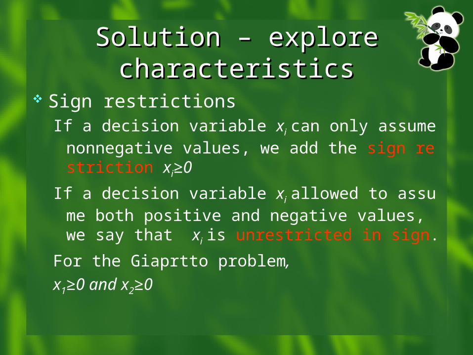
Sign restrictionsIf a decision variable xi can only assume nonne

gative values, we add the sign restriction xi≥0

If a decision variable xi allowed to assume both positive and negative values, we say that xi is unrestricted in sign.

For the Giaprtto problem,

x1≥0 and x2≥0

Solution – explore characteristicsSolution – explore characteristics

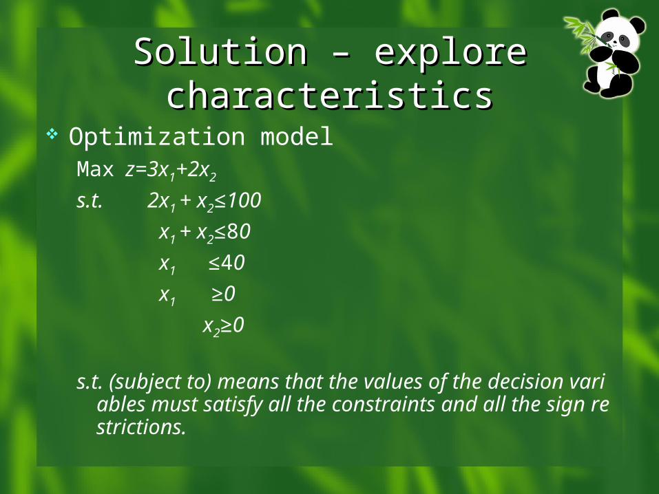
Optimization modelMax z=3x1+2x2

s.t. 2x1 + x2≤100

x1 + x2≤80

x1 ≤40

x1 ≥0

x2≥0

s.t. (subject to) means that the values of the decision variables must satisfy all the constraints and all the sign restrictions.

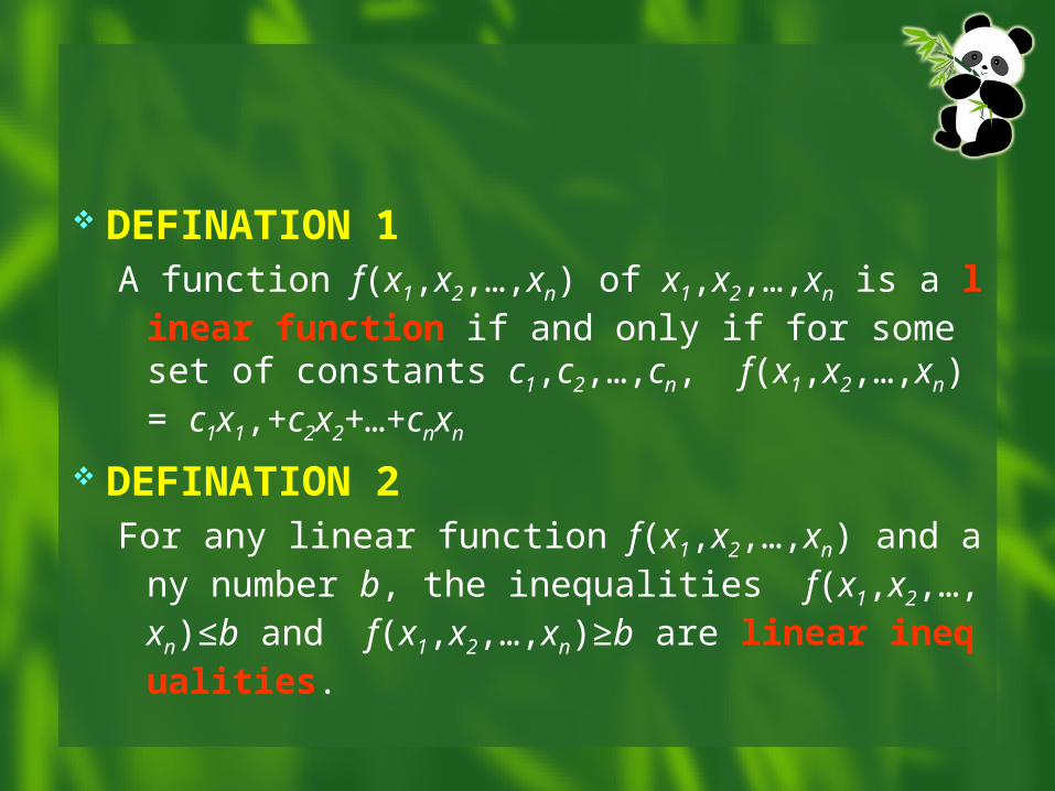
DEFINATION 1A function f(x1,x2,…,xn) of x1,x2,…,xn is a linear f

unction if and only if for some set of constants c1,c2,…,cn, f(x1,x2,…,xn) = c1x1,+c2x2+…+cnxn

DEFINATION 2For any linear function f(x1,x2,…,xn) and any nu

mber b, the inequalities f(x1,x2,…,xn)≤b and f(x1,x2,…,xn)≥b are linear inequalities.

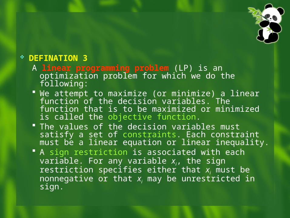
DEFINATION 3A linear programming problem (LP) is an

optimization problem for which we do the following: We attempt to maximize (or minimize) a linear

function of the decision variables. The function that is to be maximized or minimized is called the objective function.

The values of the decision variables must satisfy a set of constraints. Each constraint must be a linear equation or linear inequality.

A sign restriction is associated with each variable. For any variable xi, the sign restriction specifies either that xi must be nonnegative or that xi may be unrestricted in sign.

Feasible Region and Optimal SolutionFeasible Region and Optimal Solution

DEFINATION 4The feasible region for an LP is the set of all points

satisfying all the LP’s constraints and all the LP’s sign restrictions.

DEFINATION 5For a maximization problem, an optimal solution to

an LP is a point in the feasible region with the largest objective function value. Similarly, for a minimization problem, an optimal solution is a point in the feasible region with the smallest objective function value.

The graphical solution of two-variable The graphical solution of two-variable linear programming problemslinear programming problems Finding the feasible solution The feasible region for the Giapetto problem is the set of all points (x1.x2) satisfying all the inequalities,

2x1 + x2≤100 (Constraints) x1 + x2≤80 x1 ≤40 x1 ≥0 (Sign restrictions) x2≥0

The graphical solution of two-variable The graphical solution of two-variable linear programming problemslinear programming problems

0 20 40 60 80 1000

20

40

60

80

100

x1

x2

2 x1+x2-100 = 0

constraint 1 is satisfied

The graphical solution of two-variable The graphical solution of two-variable linear programming problemslinear programming problems

0 20 40 60 80 1000

20

40

60

80

100

x1

x2

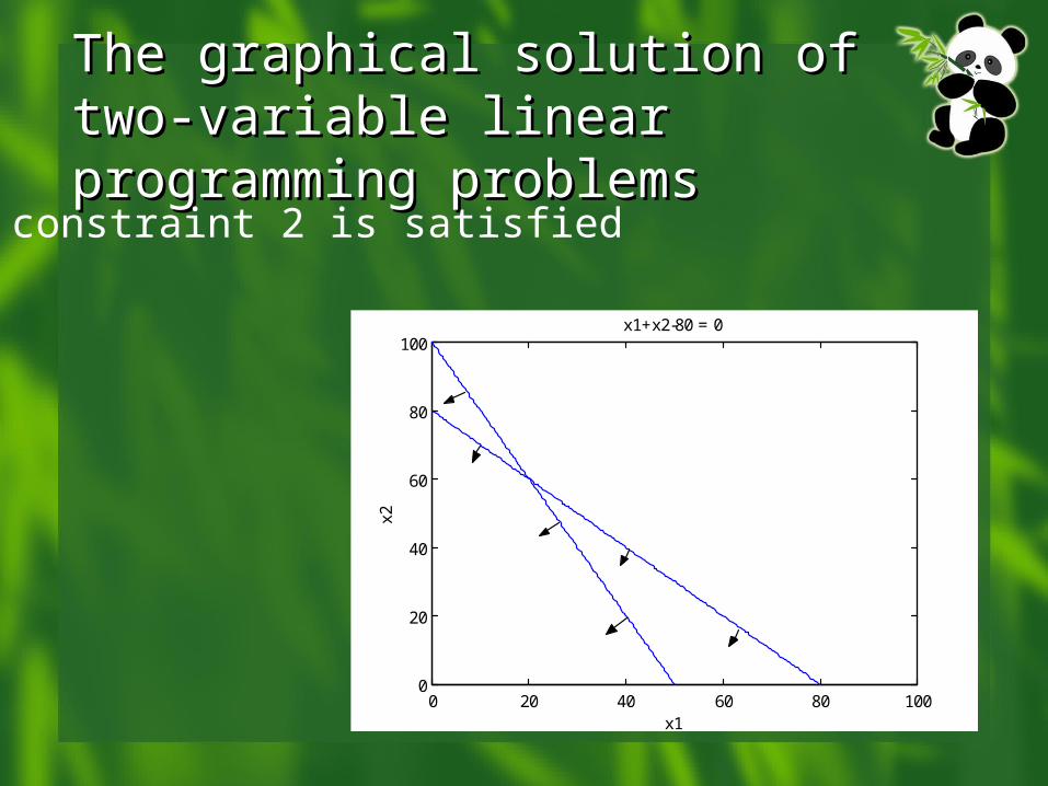
x1+x2-80 = 0

constraint 2 is satisfied

The graphical solution of two-variable The graphical solution of two-variable linear programming problemslinear programming problems

0 20 40 60 80 1000

20

40

60

80

100

x1

x2

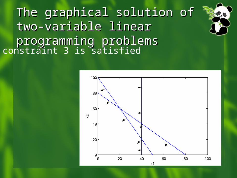
constraint 3 is satisfied

The graphical solution of two-variable The graphical solution of two-variable linear programming problemslinear programming problems

0 20 40 60 80 1000

20

40

60

80

100

x1

x2

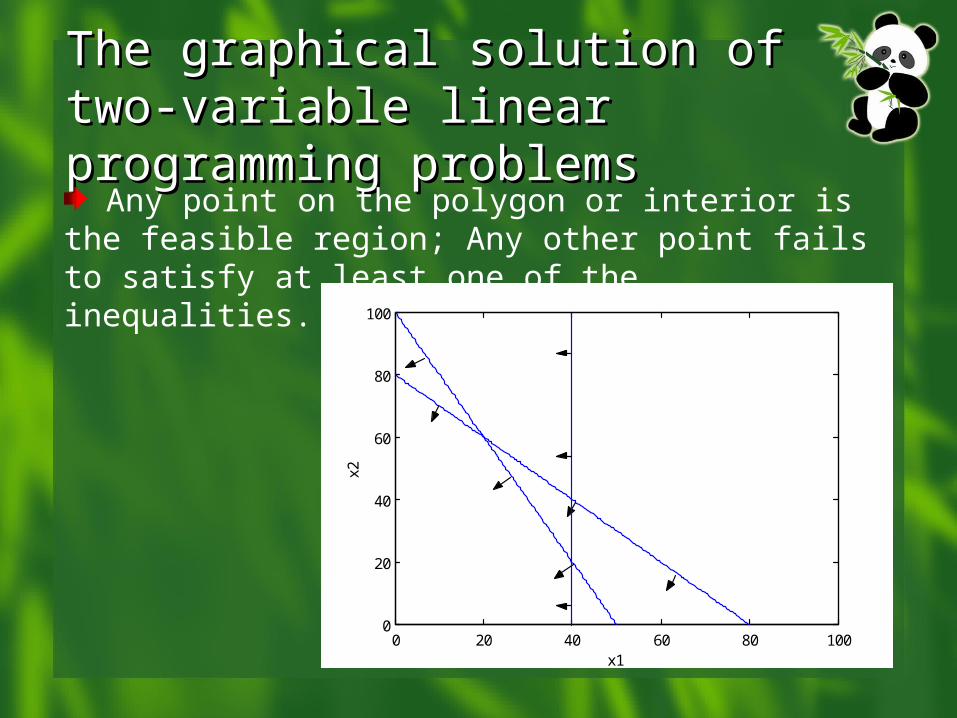
Any point on the polygon or interior is the feasible region; Any other point fails to satisfy at least one of the inequalities.

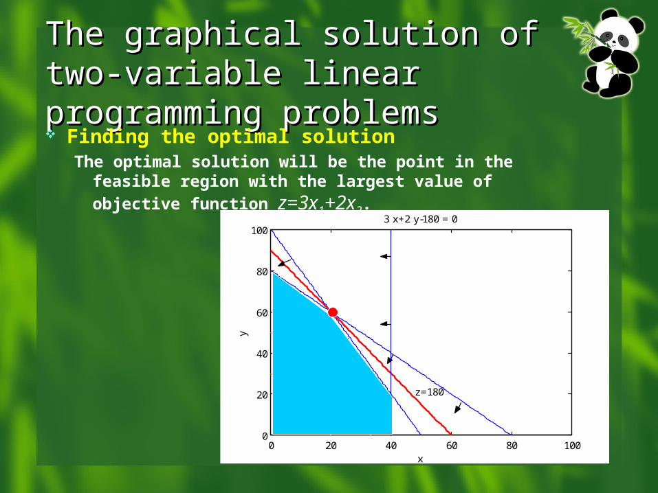
The graphical solution of two-variable The graphical solution of two-variable linear programming problemslinear programming problems Finding the optimal solution

The optimal solution will be the point in the feasible region

with the largest value of objective function z=3x1+2x2.

0 20 40 60 80 1000

20

40

60

80

100

x

y

3 x+2 y-180 = 0

z=60 z=100

z=180

Convex Sets, Extreme Points, and LPConvex Sets, Extreme Points, and LP

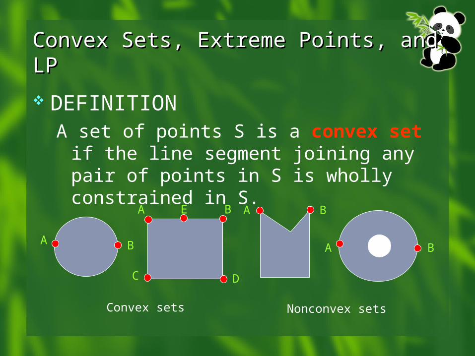
DEFINITIONA set of points S is a convex set if the line

segment joining any pair of points in S is wholly constrained in S.

Convex sets Nonconvex sets

A A

A

B B

B

E

C D

A B

Convex Sets, Extreme Points, and LPConvex Sets, Extreme Points, and LP

DEFINATION For any convex set S, a point P in S is an

extreme point (corner point) if each line segment that lies completely in S and constrains the point P has P as an endpoint of the line segment.

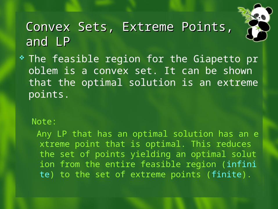
The feasible region for the Giapetto problem is a convex set. It can be shown that the optimal solution is an extreme points.

Note:

Any LP that has an optimal solution has an extreme point that is optimal. This reduces the set of points yielding an optimal solution from the entire feasible region (infinite) to the set of extreme points (finite).

Convex Sets, Extreme Points, and LPConvex Sets, Extreme Points, and LP

Special CasesSpecial Cases Three type of LPs that do not have

unique optimal solutions. Some LPs have an infinite number of optimal

solutions (alternative or multiple optimal solutions)

Some LPs have no feasible solutions (infeasible LPs)

Some LPs are unbounded: there are points in the feasible region with arbitrarily large (in a max problem) z-values.

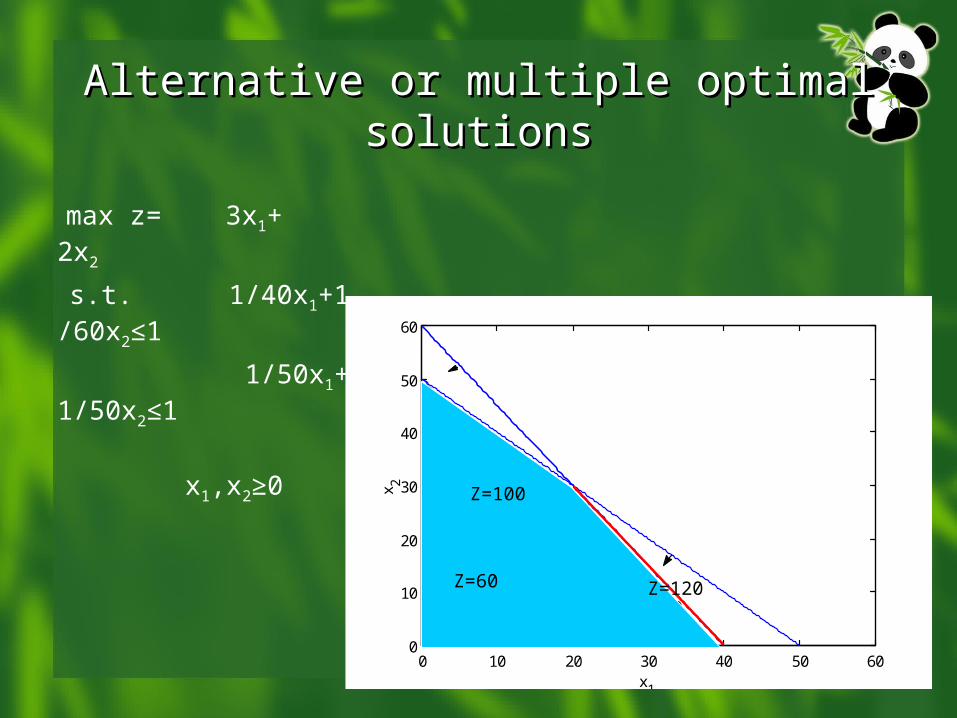
Alternative or multiple optimal solutionsAlternative or multiple optimal solutions

max z= 3x1+ 2x2

s.t. 1/40x1+1/60x2≤1

1/50x1+1/50x2≤1

x1,x2≥0

0 10 20 30 40 50 600

10

20

30

40

50

60

x1

x 2

Z=60

Z=100

Z=120

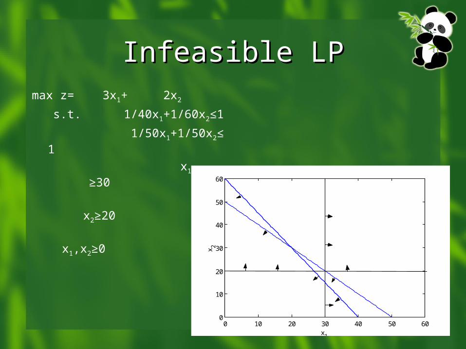
Infeasible LPInfeasible LPmax z= 3x1+ 2x2

s.t. 1/40x1+1/60x2≤1

1/50x1+1/50x2≤1

x1 ≥30

x2≥20

x1,x2≥0

0 10 20 30 40 50 600

10

20

30

40

50

60

x1

x 2

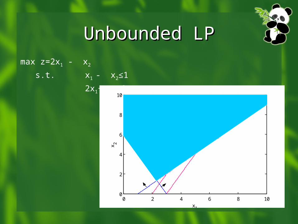
Unbounded LPUnbounded LPmax z=2x1 - x2

s.t. x1 - x2≤1

2x1+ x2≥6

x1,x2≥0

0 2 4 6 8 100

2

4

6

8

10

x1

x 2

z=6 z=4