OPTIMIZATION FRAMEWORK FOR A RADIO

FREQUENCY GUN BASED INJECTOR

by

Alicia S. HoflerB.A. May 1987, Randolph-Macon Woman’s College

M.E. August 2001, Old Dominion University

A Dissertation Submitted to the Faculty ofOld Dominion University in Partial Fulfillment of the

Requirements for the Degree of

DOCTOR OF PHILOSOPHY

ELECTRICAL AND COMPUTER ENGINEERING

OLD DOMINION UNIVERSITYMay 2012

Approved by:

Hani Elsayed-Ali (Director)

Pavel Evtushenko (Member)

Ravindra Joshi (Member)

Jiang Li (Member)

ABSTRACT

OPTIMIZATION FRAMEWORK FOR A RADIO FREQUENCYGUN BASED INJECTOR

Alicia S. HoflerOld Dominion University, 2012Director: Dr. Hani Elsayed-Ali

Linear accelerator based light sources are used to produce coherent x-ray beams

with unprecedented peak intensity. In these devices, the key parameters of the photon

beam such as brilliance and coherence are directly dependent on the electron beam

parameters. This leads to stringent beam quality requirements for the electron beam

source. Radio frequency (RF) guns are used in such light sources since they accelerate

electrons to relativistic energies over a very short distance, thus minimizing the beam

quality degradation due to space charge effects within the particle bunch. Designing

such sources including optimization of its beam parameters is a complex process

where one needs to meet many requirements simultaneously. It is useful to have a tool

to automate the design optimization in the context of the injector beam dynamics

performance. Evolutionary and genetic algorithms are powerful tools to apply to

nonlinear multi-objective optimization problems, and they have been successfully

used in injector optimizations where the electric field profiles for the accelerating

devices are fixed. Here the genetic algorithm based approach is extended to modify

and optimize the electric field profile for an RF gun concurrently with the injector

performance. Two field modification methods are used. This dissertation presents

an overview of the optimization system and examples of its application to a state

of the art RF gun. Results indicate improved injector performance is possible with

unbalanced electric field profiles where the peak field in the cathode cell is larger

than in subsequent cells.

iii

Copyright, 2012, by Alicia S. Hofler, All Rights Reserved.

iv

To my husband, Geoff, and our children, Athena and Konrad,

v

ACKNOWLEDGMENTS

I am indebted to many people for their help and support during my studies and

research leading to this dissertation. Unfortunately, I know despite my best efforts

that I will inadvertently fail to remember everyone here, and I apologize in advance

to anyone I have left out. Please know that each person’s contribution is appreciated

even if unacknowledged here.

First, I must express my extreme gratitude to my research advisors, Dr. Elsayed-

Ali and Dr. Evtushenko. They have worked tirelessly with me over the years sharing

their expertise and teaching me the research process. I have learned much from them,

and I am grateful to them.

I would like to thank Dr. Bazarov, Dr. Sinclair, and their students at Cornell

University for showing the accelerator physics community the power of evolutionary

algorithm based optimization. Their work provided a path for automating accelerator

design.

I wish to thank my committee members, Dr. Joshi and Dr. Li. They asked

provocative questions and shared their experiences with me. This helped me improve

and extend my research skills.

In the Electrical and Computer Engineering Department at Old Dominion Uni-

versity, I owe thanks to several present and past faculty members who encouraged

me to pursue graduate study. These include Dr. Gray, Dr. Gonzalez, Dr. Albin,

and Dr. Dharamsi. I also appreciate the faculty members for teaching exciting and

challenging courses. The administrative staff of the department, especially Ms. Mar-

shall, have helped me throughout. Dr. Vuskovic from the Physics Department has

shown an interest in my progress since my candidacy, and I appreciate her desire to

shepherd me through this process.

My work at Jefferson Lab piqued my interest in electrical and computer engi-

neering, and the Lab management’s strong support for education made it possible

for me to pursue my studies at Old Dominion University. I am thankful I work in an

environment filled with bright creative people eager to help anyone who shows the

slightest inclination to learn. Many past and present Jefferson Lab employees and

managers deserve my thanks for their enthusiasm and inspiration: Dr. Benesch, Mr.

Bickley, Mr. Bodenstein, Mr. Bowling, Dr. Chao, Dr. Delayen, Dr. Freyberger,

Dr. Golge, Dr. Hannon, Dr. Hutton, Dr. Kazimi, Mrs. Keesee, Dr. Kewisch, Mrs.

vi

Kjeldsen, Dr. Merminga, Dr. Poelker, Dr. Pozdeyev, Dr. Rimmer, Dr. Roblin,

Mrs. Schaffner, Dr. Shoaee, Mr. Spata, Dr. Terzic, Dr. Tiefenback, Mr. Wang,

Ms. White, and Mrs. Witherspoon. I especially want to thank Dr. Areti for his

consistent belief in me. This dissertation would not have been written without his

unflagging encouragement and support.

My parents, Linda Dickerson and the late Richard Hofler, always encouraged me

to learn and do my best. They created the foundation for this effort, and I am

eternally grateful for that. I hope to instill the same love of knowledge and learning

in my children.

Finally, I thank my husband and children who have sacrificed so much for me and

buoyed me throughout this endeavor. As my children have grown, my studies have

been a constant part of their lives. My husband has proven to be my favorite teacher.

His breadth of knowledge and gift for clear and simple explanation constantly amaze

me. I cannot thank him enough for sharing his knowledge with me and teaching me

with such grace.

Notice: This manuscript has been authored by Jefferson Science Associates, LLC

under Contract No. DE-AC05-06OR23177 with the U.S. Department of Energy. The

United States Government retains and the publisher, by accepting the article for pub-

lication, acknowledges that the United States Government retains a non-exclusive,

paid-up, irrevocable, world-wide license to publish or reproduce the published form

of this manuscript, or allow others to do so, for United States Government purposes.

vii

TABLE OF CONTENTS

Page

LIST OF TABLES . . . . . . . . . . . . . . . . . . . . . . . . . . . . . . . . . . . . . . . . . . . . . . . . . . . . . . . . . . . . ix

LIST OF FIGURES . . . . . . . . . . . . . . . . . . . . . . . . . . . . . . . . . . . . . . . . . . . . . . . . . . . . . . . . . . . x

Chapter

1. INTRODUCTION . . . . . . . . . . . . . . . . . . . . . . . . . . . . . . . . . . . . . . . . . . . . . . . . . . . . . . . . . 11.1 INTRODUCTION . . . . . . . . . . . . . . . . . . . . . . . . . . . . . . . . . . . . . . . . . . . . . 11.2 INJECTOR DESIGN PROCESS . . . . . . . . . . . . . . . . . . . . . . . . . . . . . . . . 21.3 PROPOSED APPROACH USING GENETIC ALGORITHMS . . . . . . 21.4 DISSERTATION LAYOUT . . . . . . . . . . . . . . . . . . . . . . . . . . . . . . . . . . . . . 7

2. EVOLUTIONARY ALGORITHMS OVERVIEW. . . . . . . . . . . . . . . . . . . . . . . . . . . 82.1 MULTI-OBJECTIVE OPTIMIZATION OVERVIEW . . . . . . . . . . . . . . 82.2 GENETIC AND EVOLUTIONARY ALGORITHMS OVERVIEW . . . 102.3 STRENGTH PARETO EVOLUTIONARY ALGORITHM 2 . . . . . . . . 13

3. METHODS . . . . . . . . . . . . . . . . . . . . . . . . . . . . . . . . . . . . . . . . . . . . . . . . . . . . . . . . . . . . . . . . 203.1 PURPOSE . . . . . . . . . . . . . . . . . . . . . . . . . . . . . . . . . . . . . . . . . . . . . . . . . . . 203.2 OPTIMIZATION TOOL HISTORY . . . . . . . . . . . . . . . . . . . . . . . . . . . . . . 203.3 RESEARCH ADDITIONS TO APISA . . . . . . . . . . . . . . . . . . . . . . . . . . . 253.4 COMPUTATION ENVIRONMENT CONSIDERATIONS. . . . . . . . . . . 41

4. VERIFICATION. . . . . . . . . . . . . . . . . . . . . . . . . . . . . . . . . . . . . . . . . . . . . . . . . . . . . . . . . . . 444.1 BENCHMARK INJECTOR MODEL . . . . . . . . . . . . . . . . . . . . . . . . . . . . 444.2 FIELD MORPHING . . . . . . . . . . . . . . . . . . . . . . . . . . . . . . . . . . . . . . . . . . . 564.3 CAVITY GEOMETRY MORPHING . . . . . . . . . . . . . . . . . . . . . . . . . . . . . 65

5. SUMMARY AND CONCLUSION. . . . . . . . . . . . . . . . . . . . . . . . . . . . . . . . . . . . . . . . . . 74

BIBLIOGRAPHY . . . . . . . . . . . . . . . . . . . . . . . . . . . . . . . . . . . . . . . . . . . . . . . . . . . . . . . . . . . . . 79

APPENDICES

A. ASTRA OVERVIEW . . . . . . . . . . . . . . . . . . . . . . . . . . . . . . . . . . . . . . . . . . . . . . . . . . . . . . 89A.1 INTRODUCTION . . . . . . . . . . . . . . . . . . . . . . . . . . . . . . . . . . . . . . . . . . . . . 89A.2 PHYSICAL SYSTEM TO SIMULATE . . . . . . . . . . . . . . . . . . . . . . . . . . . 89A.3 PARTICLE BASED SIMULATION . . . . . . . . . . . . . . . . . . . . . . . . . . . . . . 91A.4 EXTERNAL FIELDS . . . . . . . . . . . . . . . . . . . . . . . . . . . . . . . . . . . . . . . . . . 92A.5 INTERNAL FIELDS . . . . . . . . . . . . . . . . . . . . . . . . . . . . . . . . . . . . . . . . . . 92A.6 SOLVING THE EQUATIONS: INTEGRATION . . . . . . . . . . . . . . . . . . . 98

viii

B. POISSON SUPERFISH . . . . . . . . . . . . . . . . . . . . . . . . . . . . . . . . . . . . . . . . . . . . . . . . . . . . 100B.1 INTRODUCTION . . . . . . . . . . . . . . . . . . . . . . . . . . . . . . . . . . . . . . . . . . . . . 100B.2 DERIVATION OF GENERALIZED HELMHOLTZ EQUATION. . . . . 100B.3 DERIVATION OF EQUATION FOR FINDING RESONANCE . . . . . 105

C. APISA USER’S GUIDE. . . . . . . . . . . . . . . . . . . . . . . . . . . . . . . . . . . . . . . . . . . . . . . . . . . . 111C.1 INTRODUCTION . . . . . . . . . . . . . . . . . . . . . . . . . . . . . . . . . . . . . . . . . . . . . 111C.2 PISA CONFIGURATION AND OPERATION . . . . . . . . . . . . . . . . . . . . 111C.3 APISA SET UP . . . . . . . . . . . . . . . . . . . . . . . . . . . . . . . . . . . . . . . . . . . . . . . 114C.4 DISTRIBUTION GENERATION IN APISA . . . . . . . . . . . . . . . . . . . . . . 124C.5 APISA UPGRADE: RF CAVITY FIELD GENERATION . . . . . . . . . . 126

VITA. . . . . . . . . . . . . . . . . . . . . . . . . . . . . . . . . . . . . . . . . . . . . . . . . . . . . . . . . . . . . . . . . . . . . . . . . . 144

ix

LIST OF TABLES

Table Page

1. Example field profile characteristics provided by the field morphing method 28

2. Main solenoid settings . . . . . . . . . . . . . . . . . . . . . . . . . . . . . . . . . . . . . . . . . . . . . 45

3. Particle distribution configuration parameters . . . . . . . . . . . . . . . . . . . . . . . . 47

4. Dimensions for the three study geometries . . . . . . . . . . . . . . . . . . . . . . . . . . . 54

5. Decision variables . . . . . . . . . . . . . . . . . . . . . . . . . . . . . . . . . . . . . . . . . . . . . . . . 65

6. Linear relationship variables . . . . . . . . . . . . . . . . . . . . . . . . . . . . . . . . . . . . . . . 66

7. Geometry dimensions comparison . . . . . . . . . . . . . . . . . . . . . . . . . . . . . . . . . . . 69

8. ASTRA programs and descriptions . . . . . . . . . . . . . . . . . . . . . . . . . . . . . . . . . . 90

9. Main Poisson Superfish programs . . . . . . . . . . . . . . . . . . . . . . . . . . . . . . . . . . . 101

10. Common field generation input parameters . . . . . . . . . . . . . . . . . . . . . . . . . . . 130

11. Field morphing input parameters . . . . . . . . . . . . . . . . . . . . . . . . . . . . . . . . . . . 131

12. All field profile characteristics provided by the field morphing method . . . 132

13. Pillbox geometry example . . . . . . . . . . . . . . . . . . . . . . . . . . . . . . . . . . . . . . . . . 136

14. Re-entrant cavity geometry example based on pillbox example . . . . . . . . . . 136

15. One cell cavity with exit beam tube . . . . . . . . . . . . . . . . . . . . . . . . . . . . . . . . . 137

16. Sample ps tuner provided information . . . . . . . . . . . . . . . . . . . . . . . . . . . . . . 140

17. ps tuner arguments and descriptions . . . . . . . . . . . . . . . . . . . . . . . . . . . . . . . 141

18. xvfb manager arguments and descriptions . . . . . . . . . . . . . . . . . . . . . . . . . . . 142

x

LIST OF FIGURES

Figure Page

1. Generic injector layout . . . . . . . . . . . . . . . . . . . . . . . . . . . . . . . . . . . . . . . . . . . . 3

2. Binary crossover example . . . . . . . . . . . . . . . . . . . . . . . . . . . . . . . . . . . . . . . . . . 12

3. Probability density function for SBX. . . . . . . . . . . . . . . . . . . . . . . . . . . . . . . . 18

4. Probability density function for polynomial mutation. . . . . . . . . . . . . . . . . . 19

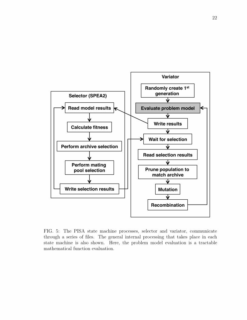
5. The PISA state machine processes, selector and variator, communicatethrough a series of files . . . . . . . . . . . . . . . . . . . . . . . . . . . . . . . . . . . . . . . . . . . . 22

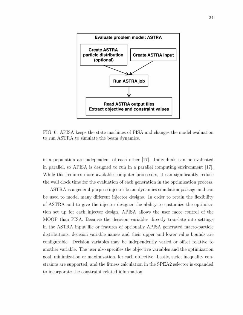
6. APISA keeps the state machines of PISA and changes the model evalua-tion to run ASTRA to simulate the beam dynamics. . . . . . . . . . . . . . . . . . . 24

7. APISA has been changed to now optionally produce a field profile for anRF cavity based gun. . . . . . . . . . . . . . . . . . . . . . . . . . . . . . . . . . . . . . . . . . . . . . 26

8. Field morphing flow chart. . . . . . . . . . . . . . . . . . . . . . . . . . . . . . . . . . . . . . . . . . 29

9. Cell geometry parameters and cavity layout . . . . . . . . . . . . . . . . . . . . . . . . . . 32

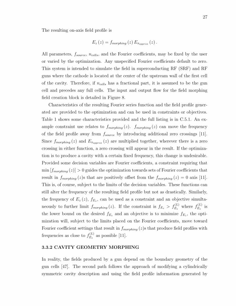
10. Straight line approximations of various cavity cell types . . . . . . . . . . . . . . . . 33

11. Examples of simple and not simple polygons. . . . . . . . . . . . . . . . . . . . . . . . . . 34

12. Cavity morphing flow chart. . . . . . . . . . . . . . . . . . . . . . . . . . . . . . . . . . . . . . . . . 36

13. Layout of front end of the PITZ diagnostic beam line . . . . . . . . . . . . . . . . . . 45

14. Field profiles used in previous work . . . . . . . . . . . . . . . . . . . . . . . . . . . . . . . . . 46

15. Spatial distributions viewed in the x−y plane for 0.45 mm rms and 0.485mm rms transverse beam sizes . . . . . . . . . . . . . . . . . . . . . . . . . . . . . . . . . . . . . . 49

16. Histograms of the plateau temporal distributions . . . . . . . . . . . . . . . . . . . . . 50

17. Momentum distribution viewed in the px − py space. . . . . . . . . . . . . . . . . . . 51

18. Momentum distribution viewed in the pz − px and pz − py spaces . . . . . . . . 51

19. PITZ curvilinear geometry . . . . . . . . . . . . . . . . . . . . . . . . . . . . . . . . . . . . . . . . . 52

20. Straight line cavity geometry using PITZ curvilinear dimensions . . . . . . . . 52

xi

21. Straight line geometry scaled to the PITZ frequency . . . . . . . . . . . . . . . . . . . 53

22. On-axis field profiles for the three cavity geometries used in the parameterscans. . . . . . . . . . . . . . . . . . . . . . . . . . . . . . . . . . . . . . . . . . . . . . . . . . . . . . . . . . . . 53

23. Average number of active particles at the end of each simulation for eachcombination of particle distribution and cavity geometry. . . . . . . . . . . . . . . 55

24. Parameter scan results for the PITZ curvilinear geometry . . . . . . . . . . . . . . 57

25. Parameter scan results for the straight line geometry . . . . . . . . . . . . . . . . . . 58

26. Parameter scan results for the scaled straight line geometry . . . . . . . . . . . . 59

27. Field morphing non-dominated individuals for several generations. . . . . . . 61

28. Ez vs. z profiles for front in first generation . . . . . . . . . . . . . . . . . . . . . . . . . . 62

29. Representative Ez vs. z profiles for front in last generation . . . . . . . . . . . . . 63

30. Details for Ez vs. z profile that gives transverse emittance 34.733 π mmmrad and spot size 25.899 mm . . . . . . . . . . . . . . . . . . . . . . . . . . . . . . . . . . . . . 64

31. Cavity geometry morphing fronts for transverse and longitudinal emittances 67

32. Cavity geometry morphing fronts for transverse emittance and beam size . 68

33. Cavity geometry morphing fronts for longitudinal emittance and beam size 68

34. Frequency for the first and last populations with members of the frontsmarked . . . . . . . . . . . . . . . . . . . . . . . . . . . . . . . . . . . . . . . . . . . . . . . . . . . . . . . . . . 70

35. Signed flatness for the first and last populations with members of thefronts marked . . . . . . . . . . . . . . . . . . . . . . . . . . . . . . . . . . . . . . . . . . . . . . . . . . . . 71

36. Field profile for cavity geometry yielding transverse and longitudinal emit-tances 2.1467 π mm mrad and 31.834 π mm keV, respectively. . . . . . . . . . . 72

37. Geometry for selected cavity geometry . . . . . . . . . . . . . . . . . . . . . . . . . . . . . . . 72

38. Cylinder and planar section for Poisson’s equation. . . . . . . . . . . . . . . . . . . . . 97

39. Probability density functions used by APISA to generate particle distri-butions. . . . . . . . . . . . . . . . . . . . . . . . . . . . . . . . . . . . . . . . . . . . . . . . . . . . . . . . . . 126

40. Cavity and beam tube layout for geometry description. . . . . . . . . . . . . . . . . 135

1

CHAPTER 1

INTRODUCTION

1.1 INTRODUCTION

For linear accelerators (linacs), the injector, where the particles to be accelerated

originate, sets the beam performance characteristics of the machine. This makes the

beam parameters at the injector a critical aspect of the final beam characteristics of

the machine. The focus of this research is, first, to develop a tool to automate the

design of injectors based on radio frequency (RF) guns and, second, to apply this

tool to examine possible improvements that can be made to an existing state of the

art RF gun.

There are two main types of electron sources or guns for photo-injectors used

in particle accelerators. The first is a direct current (DC) gun which accelerates

photo-emitted electrons using a fixed electric field between a cathode and an anode.

These guns can produce a continuous stream of electrons and are limited by field

emission [1]. They can provide the very high vacuum environments required by some

cathode photo-emitter materials [2]. A DC gun design to produce 19-77 pC electron

bunches at 1300 MHz [3] operating at a target high voltage of 750 kV is under

development at Cornell University for an energy recovery linac (ERL) based x-ray

light source [4]. It has achieved 425 kV gap voltages but operates at an administrative

limit of 250 kV [5]. Jefferson Lab’s Free Electron Laser (FEL) DC photocathode gun

has operated routinely at 320 kV, delivering 135 pC per electron bunch at 74.85

MHz [6]. The second source type is an RF gun where a time varying electric field

established in a resonance cavity structure accelerates the electrons. RF guns are

capable of accelerating 1 nC bunches of electrons to ∼4.7 MeV/c in 20 cm [7]. Due

to heat losses into the cavity walls sufficient to melt the cavity, RF guns are limited

to pulsed operation. They are also susceptible to field emission. RF guns are used

mainly in FEL light sources [8, 9].

There exist no tools to evaluate the optimality of RF gun designs thoroughly

especially with regard to the overall injector performance (beam dynamics). This

research project develops and applies an automated optimization method based on

the genetic algorithm (GA) approach to improve RF gun cavity shape based on

2

beam dynamics performance. Note that portions of this dissertation work have been

published in three conference proceedings [10–12].

1.2 INJECTOR DESIGN PROCESS

The injector for a particle accelerator typically has three main components: particle

source, beam transport system, and acceleration system. Figure 1 presents a generic

injector and its components. The overall purpose of these systems is to create a

beam at the exit of the injector that meets the specific beam quality requirements

imposed by the accelerator’s application. While it is easier to treat these systems

as independent, the reality is that the effects of these various systems become inter-

twined as the beam moves from rest at the source to typically relativistic energies at

the end of the injector. The results are systems that serve more than one function,

such as acceleration and beam transport together. This often nonlinear interplay of

effects combined with the large number of beam parameters and requirements that

sometimes conflict makes designing and optimizing an injector difficult [13]. Histor-

ically, injector optimization has been a manual process where the injector designer

concentrates on one or two beam quality requirements, designs injector components

to meet those requirements, and makes trade-offs with the balance. While injectors

designed this way are successful, it is understood that the designs may not be glob-

ally optimal, flexible, or robust over a large range of beam parameters. A system to

automate the design process could allow more than a handful of beam parameters to

be considered carefully.

The geometries of accelerating components in an injector are often selected and

optimized in an early phase of an injector design. These designs typically build on

the successes of previous machines where success is defined in terms of field char-

acteristics, mechanical stability, and manufacturability. The development cycle for

these elements is quite long. Once chosen, the injector designer must work within the

confines of the capabilities of the structures. On the other hand, it may be advanta-

geous to have the ability to explore alternative accelerating structure geometries and

their field profiles in the context of the injector design to ensure that the available

accelerating fields are best optimized to meet the injector beam requirements.

1.3 PROPOSED APPROACH USING GENETIC ALGORITHMS

Automation of the injector design and optimization process has been slow to come

3

Quadrupoles Accelerating

elements

Laser

Solenoid Photocathode

DC or RF gun

Electron beam

FIG. 1: Generic injector layout (not to scale). The particle source is comprised ofthe gun, laser, and photocathode. The gun and accelerating elements (RF cavi-ties) are the acceleration system. The beam transport consists of the magnets, butthe accelerating elements also contribute to the beam transport for non-relativisticbeams.

about for two main reasons. The first is due to the general nonlinear interdepen-

dence of beam quality parameters making it difficult to separate the variables and

treat them independently. In some cases, the relationships between parameters are

not known exactly. Posing an optimization problem using the classical methods un-

der these conditions is extremely difficult or impossible [13]. The other reason is

that the beam dynamics codes are computationally intensive. Gains in computer

processor power and speed have helped enormously allowing injector designers to

simulate many variations of a machine design in the time it took to simulate only

one or two designs over a decade ago. As is true with many physics and engineering

problems today, these simulations which were once performed on very specialized

supercomputers or large mainframe computers can now be performed on desktop

computers [14, 15]. These same gains in compute power have led to the growth of

affordable parallel computer architectures consisting of desktop class machines con-

nected with dedicated high speed networks [16]. With these dedicated distributed

computing resources, a different approach to the optimization problem taking ad-

vantage of evolutionary algorithms (EAs) or GAs can be used [17] to automate the

injector design and optimization process [13].

GAs solve problems by mimicking the way living organisms in a population pass

traits from one generation to the next through the recombination and mutation of

genes to increase the viability of the population [18, 19]. The GA approach is very

much in the vein of Darwin’s notion of “survival of the fittest” [20] where individuals

4

with the best chances of survival breed offspring with similar characteristics thereby

increasing the odds that the offspring will survive to reproduce.

GAs can be used to study problems posed as a multi-objective optimization prob-

lem (MOOP). A MOOP has several bounded inputs and more than one desired

outcome or objective. A general statement of a MOOP is [17]

Minimize/Maximize fm (x) , m = 1, 2, ...,M ;

subject to gj (x) ≥ 0, j = 1, 2, ..., J ;

hk (x) = 0, k = 1, 2, ..., K;

xi(L) ≤ xi ≤ xi

(U), i = 1, 2, ..., n;

where M , J , K, and n are, respectively, the numbers of functions to minimize or

maximize (objective functions), inequality constraint equations, equality constraint

equations, and independent or decision variables. The xi(U) and xi

(L) are the upper

and lower bounds for the decision variables. GAs are suited for MOOPs [13, 17] for

several reasons. First, unlike classical optimization methods, GAs do not require

derivative information. This is helpful for injector optimization problems where

functional information (let alone derivative) is often not available [13]. Second, they

provide a way to manage and characterize the inputs (x) and outputs of a MOOP

through decision vectors which represent different sets of values for x and fitness

assignments that indicate how well different x’s meet the constraints and optimization

objectives. Third, they can search for a set of decision vectors, x’s, that meet the

objectives and satisfy the constraints in a population if they exist.

The Platform and Programming Language Interface for Search Algorithms

(PISA) [21] provides a convenient way to merge application problems and GAs. It

separates the GA selection algorithm processing from the decision variable creation

and model evaluation processing into two programs that work in a coordinated fash-

ion using a well defined set of interface files. With this design, stand alone programs

that implement different standard GAs can be developed independently of the pro-

gram responsible for model processing. The only requirement is adherence to the file

interface, and if that is followed, the implementation details for each program are

hidden. The result is a flexible test environment where different GAs and problem

models can be used together at run time without changing the source code of either

program.

Alternate PISA (APISA) [13] is PISA where the model evaluation program has

been customized to study injectors with an interface to a beam dynamics code, viz.,

5

A Space Charge Tracking Algorithm (ASTRA) [22]. APISA is the first step towards

automating the injector design process. It allows designers to find appropriate set-

tings, magnet strengths, RF phases, and amplitudes for injector beam line elements

and the physical distances between them without changing the element geometries.

It also allows the designer to study the effect of bunch shape coming off the cathode.

For a photocathode gun, the bunch shape directly relates to the laser pulse shape

and duration. APISA has been used to determine that a high voltage DC photo-

cathode gun operating in the 500-750 kV range can serve in an injector delivering

beam meeting all of the beam quality requirements for Cornell’s proposed ERL light

source [13, 23].

This study develops a framework that allows an injector designer to optimize the

accelerating fields of an RF based electron gun concurrently with the overall injec-

tor design. This framework, based on APISA, provides two paths for gun design

development. Both approaches assume that the desired accelerating field resembles

the TM010 π-mode of a multi-cell pillbox cavity in which the phase of the acceler-

ating field changes by 180◦ in adjacent cells. The first path is a purely theoretical

exercise that searches for the on-axis accelerating electric field profile that provides

the best injector beam characteristics independent of the geometry of the gun. It

approximates the π-mode with a sine wave. It, then, changes the sine’s features by

multiplying it with a variable function described by a truncated Fourier series whose

coefficients can be changed by the GA. In reality, the fields produced by a gun depend

on the geometry of the gun cells. The second path modifies a cylindrically symmet-

ric cavity description and uses a field solver, viz., Poisson Superfish [24], to find the

attendant field profile information. The GA framework varies aspects of the cavity

description to change the field profile as dictated by the desired beam characteristics

of the injector.

An important beam characteristic for accelerators and light sources is emittance.

The particles in a charged particle bunch can be treated as a statistical ensemble. It

is more convenient to refer to the properties of the ensemble instead of the individual

particles, and the emittance is one such property. At each point in time, each particle

has six coordinates associated with it, three spatial (x, y, z) and three momenta

(px, py, pz). One way to view the ensemble of particles is in phase space. There is an

emittance for each two dimensional projection of the six dimensional phase space,

and the emittance is a measure of the area occupied by the particles in the projection.

6

The emittance is important because it is preserved under linear forces [25]. Once set

in the injector, in a linac where the linear force model applies, the emittance cannot

be improved, only degraded. The transverse rms emittance normalized with respect

to energy [26] is

εn = βγ√

⟨

(x− 〈x〉)2⟩ ⟨

(x′ − 〈x′〉)2⟩

− 〈(x− 〈x〉) (x′ − 〈x′〉)〉2

where β is v/c, v is the velocity, c is the speed of light, γ is the relativistic Lorentz

factor γ =(

√

1− β2)

−1

, x is the spatial coordinate, and x′ is the angle (x′ =

px/pz). An alternative formulation that can be used to calculate both transverse and

longitudinal emittances [27] is

εn =1

m0c

√

⟨

(px − 〈px〉)2⟩ ⟨

(x− 〈x〉)2⟩

− 〈(px − 〈px〉) (x− 〈x〉)〉2 (1)

where m0 is the particle rest mass. The emittance is fundamental to some charac-

teristics of an accelerator. In an FEL, the transverse emittance must be less than

λFEL/(4π) where λFEL is the FEL wavelength to efficiently produce radiation [28].

For light sources, emittances determine the full six dimensional normalized brightness

of the source defined as [29]

Bn =N

εn,xεn,yεn,z(2)

where N is the number of electrons in the bunch, and εn,x, εn,y, and εn,z are the

normalized transverse emittances (x,y) and the normalized longitudinal emittance

(z), respectively. The brilliance of the light produced depends on the brightness of

the source. Higher brightness leads to higher brilliance, and to increase brightness

for a fixed bunch charge, the emittances of the beam must be minimized.

The Photo Injector Test Facility Zeuthen (PITZ) [7] has developed an RF gun

based injector, and this state of the art gun is studied in this research. Its RF gun is

a 1.5 cell 1300 MHz cavity operating at 40 MV/m peak at the Cs2Te photocathode

wall. The RF cavity is located between two solenoids. The downstream solenoid is

used for emittance compensation counteracting emittance growth due to space charge

effects that develop as the electron bunch is accelerated in the cavity [30, 31]. The

upstream solenoid is used to ensure that the magnetic field at the cathode is zero.

The main requirement of this gun system is to deliver 1 nC bunches of electrons with

1-2 π mm mrad normalized transverse emittance approximately 1 m downstream of

the gun. To this end, the cavity has been tuned to produce a balanced field profile,

meaning that the amplitude of the peak field value is the same in both cells. The

7

optimizations performed in this research indicate that better transverse emittance

near the end of the injector may be achieved if the gun is operated with an unbalanced

field profile where the peak amplitude of the gun cell is twice that of the full cell.

1.4 DISSERTATION LAYOUT

This dissertation begins with an overview of GAs that covers the general terminology

and mechanisms. A description of the specific algorithm used in this research project

is included in the overview. Next, the first contribution of this dissertation research

is presented, the design and implementation of the components that automatically

generate RF cavity field profiles in APISA. This is prefaced with overviews of the

PISA and APISA systems that form its basis. Also, operational issues that impact

the design are outlined. The second contribution of this research, the analysis of

the PITZ RF gun design using this augmented version of APISA, follows. The

conclusion discusses the viability of using a GA approach in designing an RF gun

based injector and future improvements for the system. Appendices are provided for

reference. The first two describe how ASTRA, the beam dynamics simulation code,

and Poisson Superfish, the field solver, work. The third serves as a user’s guide for

PISA and APISA.

8

CHAPTER 2

EVOLUTIONARY ALGORITHMS OVERVIEW

2.1 MULTI-OBJECTIVE OPTIMIZATION OVERVIEW

When discussing MOOPs, it is helpful to understand how the problem statement

and its solutions are characterized [17]. An objective function in a MOOP is the

same as in a single objective problem. Strictly speaking, it is a function that is

to be minimized or maximized, but it can be a calculated value from a numerical

model of the system under consideration. In a multi-objective optimization, there

are two or more objectives, and they form a vector. In turn, the collection of vectors

form a space called the objective or search space. The objectives depend on a set

of variables or inputs that also form a vector known as the decision vector. Each

element in the decision vector is a decision variable with upper and lower limits on

its value. There is a corresponding decision space for the decision vectors. The

mapping between the decision and objective spaces is the mathematical model of the

system and is typically the set of objective functions to be optimized. The results of

a multi-objective optimization are presented in terms of these two spaces.

Single and multi-objective optimizations both can have constraints, and the con-

straints are used to restrict the set of candidate solutions for the optimization prob-

lem. An instance of a decision vector that falls within the limits of the decision

variables, satisfies the constraints of the problem, and is a solution of the objective

functions produces a feasible solution for the optimization. The set of all feasible

solutions for a MOOP contains both optimal and suboptimal solutions [17].

Solutions can be additionally characterized in terms of dominance. This can be

used to differentiate between the optimal and suboptimal solutions in the feasible set.

Unlike feasibility that is determined from the evaluation of the problem statement,

dominance is a relative description. It is a comparison of the objective values for two

solutions against the optimization goal. One objective value is said to be better than

another if, in the case of a minimization, its value is less than the other’s [17]. Further,

an objective value is said to be no worse than another if it is equal to or better than

the other [17,32–34]. Again, for a minimization, a solution is no worse than another

if it is less than or equal to the other. A solution, a set of objective values, dominates

9

another when all of its objective values are no worse than those of the other, and it

has at least one objective value that is better than the corresponding objective value

of the other solution. For example, in a maximization problem with six objectives, if

solution 1 has five objective values that are the same as those of solution 2 and the

remaining one is better (has a larger value), then solution 1 dominates solution 2,

and solution 2 is suboptimal relative to solution 1. Alternatively, solution 1 is said

to be non-dominated by solution 2. It is this non-dominance characteristic that is so

important in multi-objective optimization.

Because the objectives often conflict in a multi-objective optimization, it is possi-

ble to have more than one feasible optimal solution. The classic illustrative example

of conflicting objectives is car price versus features [17]. Carmakers produce cars

with a variety of interior, exterior, comfort, and safety features, and the price of a

car varies with the features provided. Why do the carmakers do this? One reason is

that they want to sell cars to as many buyers as possible, but each car buyer uses his

or her own set of criteria for choosing a car to buy. Not every car buyer can afford nor

wants a luxury car. On the flip side, there are buyers who will pay handsomely for

many features. This means there is no single best car for the carmakers to produce

in terms of cost or features. For each set of features, though, there is a price that

a buyer is willing to pay. Conversely, for each price, there is a set of features that

the carmakers are willing to provide. This leads to a set of cars not a single car to

produce. The set of cars that represents the best trade-off between cost and features

for each combination of the two is the optimal set. Ironically, there is an additional

conflict defining this best set. For the buyer, the best set may consist of the least

expensive cars for each set of features to minimize how much the buyer pays for

the most number of features. The carmaker may want to maximize profits, and the

best set may be the most expensive cars providing the least features. In reality, the

optimum where the carmaker sells the most number of cars with reasonable profits

lies in between.

Whatever the criteria for forming the best set, the optimal set has two charac-

teristics. The main one is that the members of the set are non-dominated relative to

each other. Each car price and feature pairing is the best possible for that combina-

tion. Comparing two cars in this set means their prices and features are different, but

relatively speaking, neither one is clearly better than the other. A more expensive

car from the set has the best features for that price. A cheaper car may provide

10

fewer features but still provides the best features possible at that price. Another

characteristic of the optimal set is that each member dominates at least one member

of the set of feasible solutions. In the car example, for a car buyer looking to buy

the cheapest car with the most features, an optimal car compared to the various

available cars will for the same price have more features, for the same features have

a cheaper price, or have a cheaper price and more features. This non-dominated set

is called the Pareto-optimal front [17,34]. Looking at the Pareto-optimal front in the

objective search space, it is part of the boundary surrounding the feasible solutions,

but it is not the entire boundary [17]. In the car example, the car buyer’s front

represents a different part of the search space than the carmaker’s front.

Since there may not be a single optimal solution for a MOOP, the goal of a multi-

objective optimization method is to find the Pareto-optimal front or an estimate of

it [17]. This points to the need for a method that can evaluate and process multiple

solutions concurrently to find the multiple optimal solutions and identify candidate

members of the Pareto-optimal front [17]. EAs are an appropriate choice because

they operate on populations or collections of solutions [34], and as a result, some

EAs have been specifically designed to find a broad representative sample of the

Pareto-optimal front for MOOPs.

2.2 GENETIC AND EVOLUTIONARY ALGORITHMS OVERVIEW

EAs apply processes in nature to optimization problems. GAs, a type of EA, mimic

the competition between prospective organisms to mate and the exchange and change

of genes in chromosomes during sexual reproduction to search a decision space for

optimal solutions [17]. EAs use the population and environmental pressure concepts

from evolution to direct the search toward the Pareto-optimal front. Historically,

GAs operated on binary string representations of the decision variables [18], but

that limitation seems to have eased since there are real valued vector analogs of

the processes originally designed to operate on binary strings [17]. Unless referring

specifically to the historic GAs, EA will be used throughout this discussion.

A major difference between EAs and classical optimization techniques is, as men-

tioned previously, that EAs operate on populations, a set of solutions. Classical

techniques in both single and multiple objective optimization methods are iterative

and produce a single new decision vector at the end of an iteration based on infor-

mation from a small set of previously generated solutions. In contrast, EAs produce

11

and evaluate several decision vectors per iteration, and the population of decision

and objective vectors produced during an iteration is called a generation [17]. Each

decision and objective pair is sometimes referred to as an individual [34]. Because

EAs are population based, they, also, have very novel ways to create new decision

variables.

The initial population of decision vectors is typically created by randomly select-

ing the decision variable values within the limits imposed by the optimization [17].

The general EA process starts when the decision vectors are, then, used to produce

the objective vectors, and each individual is assigned a fitness value. The fitness

metric is defined differently for each EA, and the metric is, at a minimum, a function

of the objective values. Fitness is a measure of how “good” an individual is.

The next stage is to create the next population [35]. This is a multi-step process

that mirrors to some degree what happens in biological populations. The first step is

called selection, or reproduction, where individuals deemed worthy of being parents

are identified and placed in an intermediate population known as the mating pool.

The source population from which parents are chosen varies with the algorithm but

usually is some incarnation of the previous generation. Individual worthiness is

determined by competition using fitness. There are several standard methods of

competition or selection, and each algorithm elects which one to use. Generally,

though, a selection process involves picking two individuals from a population at

random, comparing their fitness values, and putting a copy of the winner, the one

with the better fitness value, in the mating pool. The main goals of this step are

to pick the best individuals from a population to place in the mating pool, and to

ensure that better individuals have more opportunities to participate in the next step

where offspring are produced than lesser individuals. This second goal is achieved

with the number of copies a particular individual has of itself in the mating pool [17].

A better, fitter, solution should, in practice, have more copies in the mating pool

and thereby have a greater influence on the characteristics of the offspring. The net

effect of this step is to reduce the overall diversity in the offspring population [17].

Because the initial population is randomly created, it is diverse and has no preference

for any particular regions of the decision or objective space, but this is not true for

subsequent populations. The selection process introduces preferences for the regions

in the search space where the parents reside and thereby reduces the diversity of the

population [17]. This is the mechanism EAs use to identify promising regions in the

12

0 1 0 1 1 0 1 0 0 1

0 1 0 1

Parent-2 2-gene chromosome

Offspring-2 2-gene chromosome

Parent-1 2-gene chromosome

0 11 1 0 1 1 0 1 0 0 1 1 0 1 1 0 1 0 1

1 0 1 1

1 0 1 1

0 1 1 0 1 1

0 0 1 0 0 1 1 1 1 0 1 1

Offspring-1 2-gene chromosome

FIG. 2: Binary crossover example. The genes in Parent-1 in decimal are 11 and 27,and the genes in Parent-2 are 5 and 41. The first gene in each parent is transferreddirectly to the offspring. The second gene for Offspring-1 is 9 and for Offspring-2 is59.

search space.

Once the mating pool is formed, offspring are produced from the parents. Since

the original processes and terminology were developed for GAs, the discussion here

will follow suit. Recall that historically a GA works on a binary string. This string

is called a chromosome and has a fixed length [18]. The string is subdivided into

contiguous sections according to the number of decision variables, and the subsections

are called genes. Note that the string does not have to be divided into equal parts [17]

as shown in Figure 2. In this example, the chromosome is 10 bits long and has two

genes. The first gene uses 4 bits while the second uses the remaining 6 bits. Dividing

the chromosome into unequal sized genes allows one to customize the precision of each

decision variable since the number of bits allocated to a decision variable determines

the number of different available values, i.e. for an allocation of m bits, there are 2m

different values [17].

As in sexual reproduction, the chromosomes from two parents are combined to

create two new chromosomes through a process called crossover. Crossover is also

referred to as recombination. In crossover’s simplest form, single-point crossover,

two parent chromosomes are broken at the same randomly selected point in the

chromosome, and parts exchanged [18]. The break point is not confined to gene

boundaries, so whole and partial genes are exchanged in this process [17]. Figure

13

2 shows a single break occurring between bits 5 and 6 located in the second gene.

Breaking within genes creates two new chromosomes with genes that are similar to

but may not be exactly the same as the genes in the parent chromosomes. When

a partial gene is exchanged, gene information from one parent is blended with the

corresponding gene from the other parent, and the resulting offspring are variations of

the parents as is the case in Figure 2. Crossover allows GAs and EAs to move around

the decision space [17, 19]. It is analogous to swapping the y-coordinates between

two points on a 2D Cartesian plot. The two new points are displaced relative to the

original points. This is a naıve and imperfect way to create a real valued version of

this form of crossover since it respects the inherent gene boundaries in the decision

vector [17], unlike the binary version.

The other genetic process is mutation. Here, again in its simplest form, a ran-

domly selected individual bit is flipped from on to off or vice versa [17]. For a real

valued decision vector, mutation slightly adjusts a randomly picked decision variable

in the decision vector. Mutation allows the GA to increase diversity balancing the

decrease in diversity due to selection [17].

2.3 STRENGTH PARETO EVOLUTIONARY ALGORITHM 2

The algorithm used in this research, Strength Pareto Evolutionary Algorithm 2

(SPEA2) [36, 37] follows the basic processes outlined above with some variations.

SPEA2 is classified as an elite preserving algorithm. In elitist strategies, individuals

with special desirable characteristics are treated differently than members of the stan-

dard parent and offspring populations [17]. Non-dominated individuals are preferred

in SPEA2 since it strives to find a broad representative sample of the Pareto-optimal

front. Because individuals are normally chosen at random from the population to

participate in the selection competitions, it is possible that promising individuals are

overlooked and lost if they are not chosen to compete. Elitism addresses that. Since

these individuals have desirable characteristics in terms of the problem objectives,

they are kept in a reserve and allowed to outlive the generations in which they are

created. This gives them opportunities to produce offspring in subsequent gener-

ations as long as they continue to qualify as elite. They are also given preference

during the selection process for the mating pool. In SPEA2, only members of the elite

population, also known as the archive, are candidates for the mating pool [36, 37].

SPEA2 uses a fixed size archive [36, 37]. It is limited to N individuals. For each

14

new generation, after evaluating the decision vectors and assigning fitness values, it

fills the archive first with all of the non-dominated individuals from the previous con-

tents of the archive and the latest population. If the number of non-dominated indi-

viduals is larger than N , SPEA2 systematically removes less desirable non-dominated

individuals from the archive until the number of individuals matches N . Because its

archive is also the latest and best estimate of the Pareto-optimal front and is supposed

to be a diverse representation of the front, less desirable non-dominated individuals

are those that are clustered near other individuals. Clustering of solutions is a direct

consequence of the way the search in a EA focuses more tightly on the promising

regions of the search space as it progresses from one generation to the next approach-

ing the optimization goals [17]. To identify clustered individuals, SPEA2 uses the

k-th nearest neighbor distance, σk [36, 37]. Fundamentally, σk, in SPEA2, is a Eu-

clidean distance calculated in the objective space. In a list of distances calculated

between an individual i of the bloated archive and each other member of the bloated

archive sorted in increasing order, σki is the k-th element. In SPEA2, k is taken to be

√

N +N where N is the maximum size of the current population. The truncation

of the archive proceeds in rounds removing one individual each time. First, σki is

calculated for each individual i in the archive. Individuals that are either duplicates

of other individuals (have identical σk for all k) or have the same smallest σk are

identified. If a single individual is found, it is removed. Otherwise, the (k − 1)-th

distances and so on are considered until a single individual is identified. If the num-

ber of non-dominated individuals is less than the archive size, the remaining slots are

filled with the better dominated individuals from the population. Conveniently, the

fitness metric used in SPEA2 provides an indication of whether or not an individual

is non-dominated or dominated (and to what extent).

Fitness in SPEA2 is to be minimized and is calculated from three quantities [36].

The first is the strength, S(i). Strength is a tally of the number of individuals in the

archive and the current population that individual i dominates. The strength values

are then used to calculate the raw fitness, R(i), for each individual i. R(i) is the sum

of strength values, S(j), of the individuals in the archive and current population that

dominate individual i. It is zero for non-dominated individuals. The third quantity

needed for the final fitness calculation is used to differentiate between individuals

with equivalent raw fitness values. It is an estimate of the density of solutions in the

vicinity of each solution. As with the archive, the preference is to keep individuals

15

from sparser regions of the search space to maintain diversity. The density estimate

for individual i, D(i), uses σki as

D(i) =1

σki + 2

where the offset 2 is used to ensure that 0 < D(i) < 1. The fitness, F (i), is defined

as F (i) = R(i) + D(i). Referring back to the archive truncation process, for a

non-dominated individual, F (i) < 1. For dominated individuals, F (i) > 1, and

because SPEA2 fitness is to minimized, when comparing dominated individuals, the

dominated individual with F (i) closer to 1 is better.

Since dominance ranks solutions based on objective values only, SPEA2 is an un-

constrained optimization algorithm. Constrain-dominance is a ranking system that

extends the dominance definition to include the effects of inequality constraints [17].

It can be used instead of dominance in the strength and raw fitness calculation above

to change SPEA2 into a constrained optimization algorithm [13,17]. In a constrained

optimization problem, the search space is a subset of the unconstrained search space

because some feasible solutions in the unconstrained problem become infeasible in the

constrained problem [17]. Failing to satisfy one or more constraints of the constrained

problem makes these solutions infeasible in the constrained problem. Some of these

solutions may lie near the boundary between the feasible and infeasible solutions in

the constrained problem. The Pareto-optimal front for the constrained problem is a

subset of this boundary between the feasible and infeasible regions, and an infeasi-

ble solution near the boundary can provide useful constraint related information to

guide the optimization to the Pareto-optimal front. Constrain-dominance uses this

nearness to the boundary between feasible and infeasible solutions to rank infeasible

solutions [17]. An individual constrain-dominates another if any of the following three

conditions is true [17]. If its solution dominates the other under the original domi-

nance definition, constrain-dominance preserves that, and it constrain-dominates the

other. If its solution is feasible and the other is not, it constrain-dominates the other.

Lastly, if both are infeasible, then as with dominance, the constraints are compared

individually. If all of its constraints are no worse than those of the others, and it is

better in at least one constraint, then it constrain-dominates the other. Since the

original definition of dominance is preserved, the raw fitness and strength values are

unchanged for non-dominated solutions. The net effects of the change, then, are to

possibly increase the raw fitness values of dominated solutions and to provide counts

16

for infeasible solutions [17]. Since dominated solutions are feasible, their raw fit-

ness values will be less than the raw fitness values for the infeasible solutions. This

maintains the relative ranking of the solution groups: first, non-dominated solutions;

second, dominated solutions; and third, infeasible solutions.

To create offspring, this implementation of SPEA2 [21,38] uses simulated binary

crossover (SBX) [17,39,40] and uniform crossover [18] between two parents from the

mating pool, and polynomial mutation to mutate the offspring [17, 39, 40]. Uniform

crossover is an extension of the naıve single-point crossover for real valued decision

vectors discussed above in 2.2 [17]. Instead of one break point in the decision vector,

the number of possible break points is the same as the number of elements in the

decision vector. Each element of the decision vector is considered in turn and has

the opportunity to be swapped with 50 % probability [21, 38, 41].

SBX [17, 39, 40] is a better implementation of the binary form of single-point

crossover for real valued decision vectors since it incorporates the variation aspect

of binary single-point crossover. It also factors in the distance between the two par-

ents and creates similarly spaced offspring and, as a result, is an adaptive process.

Initially, the distance between pairs of parents is large since they are randomly gen-

erated, but as the search proceeds, the spacing between pairs of parents becomes

smaller as the overall population becomes less diverse. SBX defines a spread factor,

βi, between two generation t parent decision vector elements, x(1, t)i and x

(2, t)i , and

the corresponding offspring elements, x(1, t+1)i and x

(2, t+1)i , of the next generation t+1

as [17]

βi =

∣

∣

∣

∣

∣

x(2, t+1)i − x

(1, t+1)i

x(2, t)i − x

(1, t)i

∣

∣

∣

∣

∣

.

The probability density function shown in Figure 3 for achieving these spread values

based on the user configurable tuning parameter, ηSBX ≥ 0, is [17]

p (βi) =1

2(1 + ηSBX)

βηSBX

i , βi ≤ 1;

β−(2+ηSBX)i , βi > 1,

This probability density function is not symmetric about βi = 1, and its cumulative

distribution function is

P (βi) =1

2

β(1+ηSBX )i , βi ≤ 1;

−β−(1+ηSBX)i , βi > 1.

17

The Monte Carlo inverse transformation technique [42] with ui = P (βi) where ui is

a uniformly distributed random number between 0 and 1 is used to generate random

[17, 39, 40]

βri =

{2ui}(

11+ηSBX

)

, ui ≤ 12;

{2 (1− u)}(

−11+ηSBX

)

, ui >12.

Finally, the offspring x(1, t+1)i and x

(2, t+1)i are linear combinations of the parents with

βri scaling factors [40]

x(1, t+1)i =

1

2

{(

x(1, t)i + x

(2, t)i

)

+ βri

(

x(1, t)i − x

(2, t)i

)}

, (3)

x(2, t+1)i =

1

2

{(

x(1, t)i + x

(2, t)i

)

− βri

(

x(1, t)i − x

(2, t)i

)}

. (4)

This assumes the decision vectors are not bounded [40]. For bounded decision vectors,

the spread is redefined to ensure that the offspring created fall within the bounds of

the decision variable. The bounded version of the spread, βi, is defined relative to

the upper and lower bounds on the decision variable, x(U)i , and x

(L)i as [39, 40]

βi = 1 + 2min

(

x(1, t)i − x

(L)i , x

(2, t)i − x

(L)i , x

(U)i − x

(1, t)i , x

(U)i − x

(2, t)i

)

∣

∣

∣x(2, t+1)i − x

(1, t+1)i

∣

∣

∣

.

The randomly generated βr

i is [39, 40]

βr

i =

(αui)

(

11+ηSBX

)

, ui ≤ 1α;

{2− αui}(

−11+ηSBX

)

, ui >1α.

where α = 2− β−(1+ηSBX )

i , and βr

i is used in (3) and (4) instead of βri .

Polynomial mutation is similar to SBX in that it is uses a customizable probability

density function to create a small offset that is added to a randomly selected variable

in the decision vector [17]. Polynomial mutation, also, has bounded and unbounded

implementations. The unbounded probability density function shown in Figure 4 is

a polynomial function with the user defined tuning parameter, ηpm ≥ 0, [17, 39, 40]

p (δi) =1

2(1 + ηpm) (1− |δi|)ηpm .

This function is symmetric about δi = 0. For uniformly distributed ui between 0 and

1, the randomly generated [17, 40]

δri =

(2ui)

(

11+ηpm

)

− 1, ui <12;

1− {2 (1− ui)}(

11+ηpm

)

, ui ≥ 12.

18

0

2

4

6

8

10

12

0 0.5 1 1.5 2

Sim

ulat

ed b

inar

y cr

osso

ver

(SB

X)

p.d.

f.

βi

ηSBX=1ηSBX=10ηSBX=20

FIG. 3: Probability density function for SBX.

are used in

xi(1, t+1) = x

(1, t+1)i + δri∆max

to create the mutated, xi(1, t+1), from x

(1, t+1)i where ∆max is the maximum change

allowed. The next generation index, t + 1, is used on both sides of the equation

because mutation occurs after crossover, and crossover creates two new individuals

for the next generation. This means that mutation is modifying a member of the

next generation. The bounded versions are [39, 40]

∆max = x(U)i − x

(L)i

and

δr

i =

(

2ui + (1− 2ui) (1− δ)1+ηpm)

(

11+ηpm

)

− 1, ui <12;

1−{

2 (1− ui) + 2(

ui − 12

)

(1− δ)1+ηpm}

(

11+ηpm

)

, ui ≥ 12.

where

δ =min

(

x(1, t+1)i − x

(L)i , x

(U)i − x

(1, t+1)i

)

x(U)i − x

(L)i

.

19

0

2

4

6

8

10

12

-1 -0.5 0 0.5 1

Pol

ynom

ial m

utat

ion

p.d.

f.

δi

ηpm=1ηpm=10ηpm=20

FIG. 4: Probability density function for polynomial mutation.

20

CHAPTER 3

METHODS

3.1 PURPOSE

This study develops a framework that allows an injector designer to optimize the

accelerating fields of an RF based electron gun concurrently with the overall injector

design. This framework, based on APISA [13] from Cornell University, provides two

paths for the gun design. Both approaches assume that the desired accelerating field

resembles the π mode (TM010) of a multi-cell pillbox cavity where the phase of the

accelerating field changes by 180◦ in adjacent cells. Two ancillary goals of this project

are to make a system that is of general use and to use free or freely available software

solutions.

3.2 OPTIMIZATION TOOL HISTORY

In this section, the foundations for the optimization software design and operation

are described. APISA is an extension of PISA [21] from the Computer Engineering

and Networks Laboratory (TIK) of the Swiss Federal Institute of Technology (ETH)

Zurich. Therefore, PISA is discussed first followed by APISA.

3.2.1 PISA

PISA is a software package to use for easily evaluating the performance of various

GAs and EAs against known or standard academic unconstrained MOOPs [36]. For

reference, the general statement of this type of MOOP is

Minimize/Maximize fm (x) , m = 1, 2, ...,M ;

subject to xi(L) ≤ xi ≤ xi

(U), i = 1, 2, ..., n;

where x is a vector of n decision variables with upper and lower bounds, x(U)i and

x(L)i , and fm (x) are the M objective functions to optimize. While EAs differ in

implementation and strategy for searching a decision variable space, they share a

basic function to identify individuals in a population to seed the next generation of

decision variable vectors. PISA takes advantage of this commonality to divide the

process into two state machines that communicate through files [21,38,41] as shown

21

in Figure 5. One state machine identifies individuals for the mating pool and archive,

and the other performs problem evaluations and generates individuals. These state

machines operate under the assumption that only one state in one state machine is

active at a time, and processing is coordinated with a file that acts like a semaphore.

The identification state machine, referred to as the selector [21,38,41], is the key

to the success of the optimization despite its relative simplicity. Its main function is

to identify individuals in the population to put in the mating pool. At a minimum

this process involves calculating a fitness value for each individual in the population

and selecting potential parents based on fitness and other criteria outlined in the

algorithm. For algorithms like SPEA2, the selector also identifies members of the

archive. All of the steps in the selector can be performed without specific knowledge

of the problem under consideration because the fitness calculation is based on domi-

nance, the relative comparison of objective values only. This means that the selector

needs only objective value related information to complete its task. Specifically, it

needs the total number of objective functions to consider and, for each individual,

the identity information (i.e., index identification number) and the objective values.

The variator state machine provides overall control of the progression of the op-

timization and does the bulk of the work [21, 38, 41]. It keeps track of the number

of generations that have run and checks for completion. It creates individuals for

the population either randomly for the first generation or through recombination

and mutation applied to the contents of the mating pool. Each new individual then

translates into a problem model evaluation to obtain new objective values. Other

information from the selector state machine such as the contents of the archive may

require the variator to prune individuals from the population.

Since PISA’s purpose is to study benchmark unconstrained MOOPs [41], the vari-

ator has a list of predefined problems with known multi-variable objective functions

that it can optimize. The limits of the decision variable values are automatically

generated for each problem. The predefined problems and generated decision vectors

simplify the optimization problem configuration. Running an optimization requires

the name of the problem to solve, the numbers of decision variables and objective

functions to use, the maximum number of generations to produce, and quantities

related to population size. The maximum number of generations is used to stop

optimization processing, and the output is the decision and objective information for

the individuals that form the best approximation of the Pareto-optimal front.

22

Selector (SPEA2)

Read model results

Perform archive selection

Write selection results

Calculate fitness

Perform mating pool selection

Variator

Read selection results

Evaluate problem model

Randomly create 1st generation

Write results

Mutation

Recombination

Prune population to match archive

Wait for selection

FIG. 5: The PISA state machine processes, selector and variator, communicatethrough a series of files. The general internal processing that takes place in eachstate machine is also shown. Here, the problem model evaluation is a tractablemathematical function evaluation.

23

PISA allows the user to control aspects of these randomized processes used in

creating new individuals. There are gatekeeper parameters that are used to determine

whether or not a process such as recombination or mutation will occur at all for an

individual. In each application of the process, a random number is generated and

compared to the gatekeeper threshold provided. If the generated number is less

than or equal to the threshold, the process is allowed. The η parameters used in

probability density functions for operations like SBX and polynomial mutation are

user configurable.

The basic purpose, design, and operation of PISA have been covered.

3.2.2 CORNELL’S APISA

APISA [13] is PISA that has been customized for accelerator injector design since

its variator runs ASTRA, an accelerator beam dynamics simulation program, and it

uses ASTRA results to compute its objective function values. Figure 6 shows the

details of the problem evaluation block in APISA that interfaces to ASTRA. Merging

PISA and ASTRA enables injector designers to vary several parameters including the

characteristics of the bunch emitted from the source, operating settings for beam line

elements (e.g., amplitudes and phases), and the relative spacing of the elements in

the beam line simultaneously to find optimized injector designs. Because APISA

allows constraints [13], it solves a more general MOOP for injector designs

Minimize/Maximize fm (x) , m = 1, 2, ...,M ;

subject to gj (x) > g(L)j , j = 1, 2, ..., J ′;

gj (x) < g(U)j , j = (J ′ + 1), (J ′ + 2), ..., J

x(L)i ≤ xi ≤ x

(U)i , i = 1, 2, ..., n;

where g(L)j and g

(U)j are the bounds used in the strict inequality constraints.

PISA is designed to work with small and relatively simple problems that can

be evaluated easily and very quickly, so it performs all calculations serially without

a noticeable impact on execution time. Beam dynamics simulations are more CPU

intensive by nature because they model the response of many charged macro-particles

to the electromagnetic fields in an injector beam line. The execution time of a beam

dynamics simulation increases with the number of macro-particles, the length of the

beam line modeled, and the complexity and number of electromagnetic fields. For

this reason, APISA takes advantage of the fact that once defined all individuals

24

Evaluate problem model: ASTRA

Create ASTRA input

Run ASTRA job

Read ASTRA output files Extract objective and constraint values

Create ASTRA particle distribution

(optional)

FIG. 6: APISA keeps the state machines of PISA and changes the model evaluationto run ASTRA to simulate the beam dynamics.

in a population are independent of each other [17]. Individuals can be evaluated

in parallel, so APISA is designed to run in a parallel computing environment [17].

While this requires more available computer processors, it can significantly reduce

the wall clock time for the evaluation of each generation in the optimization process.

ASTRA is a general-purpose injector beam dynamics simulation package and can

be used to model many different injector designs. In order to retain the flexibility

of ASTRA and to give the injector designer the ability to customize the optimiza-

tion set up for each injector design, APISA allows the user more control of the

MOOP than PISA. Because the decision variables directly translate into settings

in the ASTRA input file or features of optionally APISA generated macro-particle

distributions, decision variable names and their upper and lower value bounds are

configurable. Decision variables may be independently varied or offset relative to

another variable. The user also specifies the objective variables and the optimization

goal, minimization or maximization, for each objective. Lastly, strict inequality con-

straints are supported, and the fitness calculation in the SPEA2 selector is expanded

to incorporate the constraint related information.

25

As an aside, APISA employs simple arithmetic tricks [17] to concurrently ac-

commodate minimization, maximization, and both kinds of strict inequality con-

straints [17]. A maximization problem can be converted into a minimization problem

by multiplying the objective value by -1 and looking for the corresponding minimum

objective value. Similarly, a less than constraint can be converted to a greater than

constraint by first changing the constraint to be relative to zero and then again mul-

tiplying through by -1. Stated more explicitly for an arbitrary constraint variable,

gj (x), whose value must be less than g(U)j :

gj (x) < g(U)j

gj (x)− g(U)j < 0

−(

gj (x)− g(U)j

)

> 0

g(U)j − gj (x) > 0.

With these two conversions, APISA reduces all problems to minimizations that are

subject to strictly greater than constraints. Thus the same fitness calculation can be

used for any combination of objective goals and constraints types.

3.3 RESEARCH ADDITIONS TO APISA

The two cavity field generation extensions to APISA and additional minor features

developed for this research are covered in this section. Also, an overview of the op-

erating environment and its impacts on the design and execution of the optimization

system are provided.

To provide APISA with the ability to modify the fields provided by an RF based

gun as part of an injector optimization, APISA has two methods for creating field

profiles. Figure 7 shows where in the problem evaluation block the field creation

systems have been added. The first method, called field morphing, morphs an ideal-

ized field profile using a truncated Fourier series [11]. This creates nonphysical field

profiles since boundary conditions are ignored, but it can find field profile shapes

that can be used to guide cavity geometry development. The second method, called

geometry morphing, modifies a cavity geometry and uses a field solver to generate

the field profile [11, 12]. For each field generation method, relevant characteristic

information that can be used in the optimization as constraints or objectives is pro-

vided. These two field generation methods and additional supporting features are

discussed next.

26

Evaluate problem model: ASTRA and optional cavity field creation

Create ASTRA input

Run ASTRA job

Read ASTRA and field profile output files Extract objective and constraint values

Create field profile

(optional)

Create ASTRA particle distribution

(optional)

FIG. 7: APISA has been changed to now optionally produce a field profile for an RFcavity based gun.

3.3.1 FIELD MORPHING

In this purely theoretical method, the field profile for the field morphing method is

derived from a sine wave with frequency, fsource. This sine wave, Eπapprox, roughly

approximates the accelerating π mode in a cavity and is defined as

Eπapprox(z) = sin

(

2πz

λsource

)

with free space wavelength, λsource = c/fsource. Eπapprox(z) is combined with a trun-

cated Fourier series to create an on-axis field profile, Ez (z), to use in ASTRA. The

truncated Fourier series is

fmorphing (z) = 1 +

15∑

n=1

an cos

(

2πnz

Lcavity

)

+

15∑

n=1

bn sin

(

2πnz

Lcavity

)

where Lcavity is the length of the cavity. The 1 in the fmorphing (z) expression ensures

that the resulting field profile reproduces Eπapprox(z) when all of the Fourier coeffi-

cients are zero. Lcavity is found from λsource and the number of cells in the RF cavity,

ncells, so

Lcavity = ncells

λsource

2.

27

The resulting on-axis field profile is

Ez (z) = fmorphing (z)Eπapprox(z) .

All parameters, fsource, ncells, and the Fourier coefficients, may be fixed by the user

or varied by the optimization. Any unspecified Fourier coefficients default to zero.

This system is intended to simulate the field in superconducting RF (SRF) and RF

guns where the cathode is located at the center of the upstream wall of the first cell

of the cavity. Therefore, if ncells has a fractional part, it is assumed to be the gun

cell and precedes any full cells. The input and output flow for the field morphing

field creation block is detailed in Figure 8.

Characteristics of the resulting Fourier series function and the field profile gener-

ated are provided to the optimization and can be used in constraints or objectives.

Table 1 shows some characteristics provided and the full listing is in C.5.1. An ex-

ample constraint use relates to fmorphing (z). fmorphing (z) can move the frequency

of the field profile away from fsource by introducing additional zero crossings [11].

Since fmorphing (z) and Eπapprox(z) are multiplied together, wherever there is a zero

crossing in either function, a zero crossing will appear in the result. If the optimiza-

tion is to produce a cavity with a certain fixed frequency, this change is undesirable.

Provided some decision variables are Fourier coefficients, a constraint requiring that

min [fmorphing (z)] > 0 guides the optimization towards sets of Fourier coefficients that

result in fmorphing (z)s that are positively offset from the fmorphing (z) = 0 axis [11].

This is, of course, subject to the limits of the decision variables. These functions can

still alter the frequency of the resulting field profile but not as drastically. Similarly,

the frequency of Ez (z), fEz, can be used as a constraint and an objective simulta-

neously to further limit fmorphing (z). If the constraint is fEz> f

(L)Ez

where f(L)Ez

is

the lower bound on the desired fEzand an objective is to minimize fEz

, the opti-

mization will, subject to the limits placed on the Fourier coefficients, move toward

Fourier coefficient settings that result in fmorphing (z)s that produce field profiles with

frequencies as close to f(L)Ez

as possible [11].

3.3.2 CAVITY GEOMETRY MORPHING

In reality, the fields produced by a gun depend on the boundary geometry of the

gun cells [47]. The second path follows the approach of modifying a cylindrically

symmetric cavity description and using the field profile information generated by

28

TABLE 1: Example field profile characteristics provided by the field morphingmethod

Characteristic Method of Calculation

Maximum of Ez (z) max [Ez (z)]

Minimum of Ez (z) min [Ez (z)]

Frequency of Ez (z), fEzFrequency of Ez (z) determined viaFast Fourier Transform [43–46]

Maximum of fmorphing (z) max [fmorphing (z)]

Minimum of fmorphing (z) min [fmorphing (z)]

the field solver Poisson Superfish [24] from Los Alamos National Laboratory. Since

this method uses solutions to Maxwell’s equations for physical cavity geometries

and boundary conditions, the field profiles produced are more realistic than the

idealized field profiles of the field morphing method. This section discusses how

Poisson Superfish is incorporated into APISA. There are three parts. The first is a

general cavity geometry description with named parts that can be easily modified

by the optimization software. The second component is a translation that converts

the geometry description to Poisson Superfish’s geometry description. Lastly, there

is a set of programs that encapsulates the Poisson Superfish processing to produce

a field profile to use in ASTRA simulations and a list of cavity field characteristics

and figures of merit for the optimization to use in constraints and objectives. These

will all be discussed in turn following a brief overview of Poisson Superfish and its

suitability for this optimization system.

Poisson Superfish overview

Poisson Superfish [48] is a field solver commonly used in accelerator physics to calcu-

late electromagnetic fields for RF cavities and magnets. It is written in FORTRAN.

It uses the FORTRAN namelist input format and produces binary formatted and

text output. For RF cavities, it assumes the geometry is cylindrically symmetric.

This means it only needs a description of the cross-section of the top half of the cav-

ity geometry to find the fields in the cavity. It creates physical and logical triangular

meshes on which it solves the Helmholtz equation to calculate the fields (discussed in

B.2). A fictitious magnetic current density is used to excite the fields in the cavity.

29

Create field profile with field morphing (optional)

Compute field profile

Write out field profile and characteristic features

Default an’s

and bn’s

Decision variable an’s and b

n’s

Compute characteristic features

fsource

, number of cells, number of points in profile

FIG. 8: Field morphing flow chart.

On resonance, when the energy transfer between the electric and magnetic fields is

balanced, this magnetic current density goes to zero as it should. It, also, calculates

several characteristics of the field and figures of merit.

There are several benefits to using Poisson Superfish. The first is that it is freely

available in the United States [24]. This satisfies a goal of this optimization software

design to use free or essentially free software. It is a standard in the accelerator

community and has long been used to design and model RF cavities. It computes

the fields and characteristics fairly quickly making it a good candidate field solver to

use in a system that needs to calculate the fields for hundreds of cavity geometries

per generation in a timely fashion.

From the standpoint of running the optimization, the main drawback to Poisson

Superfish is that, while it once ran on several different platforms including linux, it

now runs only in a Windows environment [15]. The optimization software is designed

to run in a linux environment since at present virtually all large-scale computing

facilities are linux based. This means some software framework is needed to enable

30

Poisson Superfish to run under linux. The solution to this using Wine [49,50], a freely

available environment for running Windows executables in other operating system

environments, and Xvfb [51,52], the X Windows virtual frame buffer, is discussed in

detail subsequently.

Cavity description

A Poisson Superfish geometry description is essentially an ordered list of points,

lines, and curves that form a set of closed areas that represent a cross-section of the

electromagnetic field producing device [48]. The very general nonspecific nature of

the description poses challenges for incorporating it into the optimization software.

Examples of the challenges and the solution used in this research to address them

are presented.

Without plotting the lines and curves in a Poisson Superfish geometry description,

it is not always obvious what shape or shapes the geometry description represents.

Further, for RF cavity representations, matching the lines and curves of the geometry

description to the physical parts of a cavity can be difficult, even for simple designs,

because the geometry description provides no clues as to what part of the cavity

structure a set of lines and curves depicts. For the optimization software to change

the geometry description directly, it needs to be able to automate this identification

process. For example, to change the radius of one cell in a multi-cell cavity, the

optimization first needs to know which parts of the description are associated with

the particular cell to be changed. It then needs to know which subset of those lines

and curves depend on the radius of the cell. Finally, it has to compute changes for

each of these elements and generate a new geometry description. This requires some

a priori knowledge of the desired final cavity shape and restrictions on how the lines,

points, and curve elements are used to create it. This can lead to limitations on the

types of cavities that the optimization can be applied to since the specifics of each

cavity type have to be translated into a set of rules that the optimization can use to

identify the cavity type and its components [48].

Because the lines and curves in the ordered list use a combination of absolute and

relative position information [48], another complication is that adding or making a

change to one part of the description may require changes to all downstream com-

ponents. For example, increasing the length of a cavity cell shifts the positions of

downstream elements, and those positions must also be updated. Unlike the radius

31

change example above where the changes are limited to the cell to be changed, this

simple cell length change is not localized. This can be further complicated if there

is interplay resulting from other changes.

These challenges can be recast differently. Although not explicitly stated, the

optimization needs a name for what it will change in the cavity geometry to fit in

the decision vector model [12]. It also needs to know how to propagate that named

change into the many possible required changes in the geometry description. The

foregoing discussion outlines the challenges related to designing the optimization

to directly manipulate the Poisson Superfish geometry description. The solution

then is to separate the details of Poisson Superfish’s geometry description from the

optimization software. This can be accomplished with a cavity description based on

cavity structural elements and their dimensions that can be translated into a Poisson

Superfish geometry description.

This cavity geometry description assumes cavities are built from two elements,

tubes and cells [12]. The cell parameters are shown in Figure 9. Each self-contained

element is named and is described by a list of named dimensions, offsets, and angles.

The cavity is, then, described with an ordered list of these cavity building blocks that

are together converted to a Poisson Superfish file. The first benefit of this description

approach is that each aspect of the cavity geometry has a name. It also makes it

easy to change or add elements to the description since the individual elements are

independent of each other. Adding or changing a building block element may require

minor changes to neighboring elements, but the changes only involve simple value

substitutions and are limited to the elements on either side. For example, if the

radius of a beam tube is changed, it may be necessary to change the exit iris radius

of the upstream cavity element and the entrance iris radius of the downstream ele-

ment. Otherwise, adding an element is just a matter of inserting the building block

describing the element in the appropriate position in the description. The optimiza-

tion though does not add or remove building blocks. For each optimization, the

number, types, and order of the building blocks are fixed. However, the optimiza-

tion can change settings in the description, and using a feature described in 3.3.3

and C.5.2, it can perform any related substitutions as directed in the optimization

decision variable configuration.

Although the geometry translation only produces straight-line cavity geometries

[11,12], the cavity geometry description is flexible and allows the geometry of a cavity

32

Cell radius

Neck width

Cell base width

Cell offsets

Radii of irises

Neck offsets

Entrance wall Exit wall

Cell wall angles -90o < θ < 90o

FIG. 9: Cell geometry parameters and cavity layout [12].

to morph easily from one general form to another. The main cavity cell type used in

this research is the pillbox cavity used in RF guns, and it can be extended easily to

its elliptical cavity counterpart used in SRF guns. Both of these geometries produce

simple accelerating mode fields. A pillbox cell can be described simply by its radius

and length since it is a right cylinder. Because the cavity description is designed to

produce the features of several cavity types, it contains more dimensions than the

radius and length, and these have to be set for completeness. A rough approximation

of an elliptical cavity can be made from a pillbox cavity if the walls or end caps are

allowed to tilt toward each other. Another cavity type, called re-entrant, can be

modeled with the end cap cones tilted away from each other. Examples of all three

are shown in Figure 10.

Some Poisson Superfish specific information is included in the geometry descrip-

tion because the information is necessary to the operation of Poisson Superfish [48].

The first is related to frequency. In Poisson Superfish, the FREQ namelist variable is

often thought of as the desired resonance frequency of the geometry, but it is sub-

tly different from that. In reality it is used by Poisson Superfish to decide where to

search for the resonance frequency [48]. Often, it turns out that this search frequency

is the resonance frequency, but it is not guaranteed. The frequency building block in

this description is used in the same way and is referred to as the search frequency.

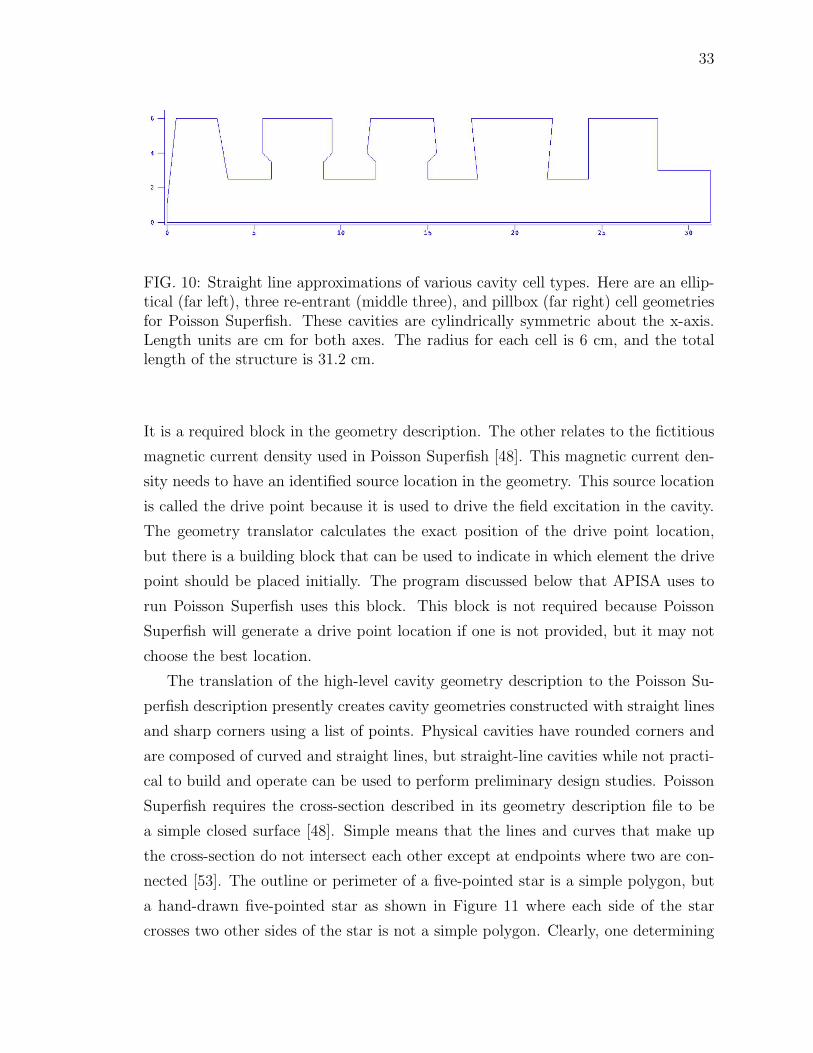
33

FIG. 10: Straight line approximations of various cavity cell types. Here are an ellip-tical (far left), three re-entrant (middle three), and pillbox (far right) cell geometriesfor Poisson Superfish. These cavities are cylindrically symmetric about the x-axis.Length units are cm for both axes. The radius for each cell is 6 cm, and the totallength of the structure is 31.2 cm.

It is a required block in the geometry description. The other relates to the fictitious

magnetic current density used in Poisson Superfish [48]. This magnetic current den-

sity needs to have an identified source location in the geometry. This source location

is called the drive point because it is used to drive the field excitation in the cavity.

The geometry translator calculates the exact position of the drive point location,

but there is a building block that can be used to indicate in which element the drive

point should be placed initially. The program discussed below that APISA uses to

run Poisson Superfish uses this block. This block is not required because Poisson

Superfish will generate a drive point location if one is not provided, but it may not

choose the best location.

The translation of the high-level cavity geometry description to the Poisson Su-

perfish description presently creates cavity geometries constructed with straight lines

and sharp corners using a list of points. Physical cavities have rounded corners and

are composed of curved and straight lines, but straight-line cavities while not practi-

cal to build and operate can be used to perform preliminary design studies. Poisson

Superfish requires the cross-section described in its geometry description file to be

a simple closed surface [48]. Simple means that the lines and curves that make up

the cross-section do not intersect each other except at endpoints where two are con-

nected [53]. The outline or perimeter of a five-pointed star is a simple polygon, but

a hand-drawn five-pointed star as shown in Figure 11 where each side of the star

crosses two other sides of the star is not a simple polygon. Clearly, one determining

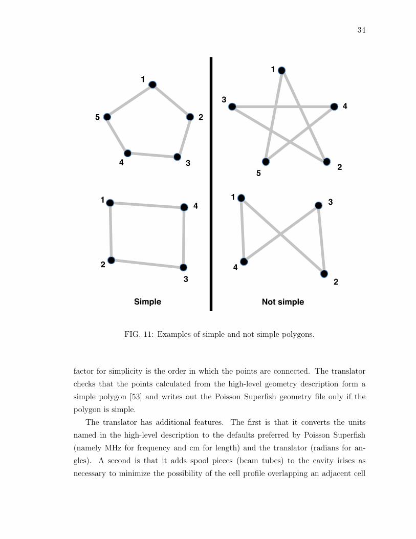
34

4

1

2

3

5

1

5

3

2

4

1

2

3

41

2

3

4

Simple Not simple

FIG. 11: Examples of simple and not simple polygons.

factor for simplicity is the order in which the points are connected. The translator

checks that the points calculated from the high-level geometry description form a

simple polygon [53] and writes out the Poisson Superfish geometry file only if the

polygon is simple.

The translator has additional features. The first is that it converts the units

named in the high-level description to the defaults preferred by Poisson Superfish

(namely MHz for frequency and cm for length) and the translator (radians for an-

gles). A second is that it adds spool pieces (beam tubes) to the cavity irises as

necessary to minimize the possibility of the cell profile overlapping an adjacent cell

35

and creating a non-simple cross-section. This is useful for re-entrant style cavities

that have dumbbell shaped cross-sections. Lastly, it identifies potential cavity sec-

tions for drive point placement and calculates drive point positions.

For APISA, the geometry translation and Poisson Superfish processing are com-

bined into one program called ps_tuner [12]. The field creation block with ps_tuner

for cavity morphing is shown in Figure 12. Basically, this program takes a geometry

description as an input and produces a field profile and relevant characteristics. It

aims to find a π mode, but if it is unsuccessful, it provides a minimal Ez (z) = 0

profile. The search for the π mode is a multi-step process. First, it determines

which elements in the geometry description can be used for drive point locations.

If a drive point location is provided, it is placed first in the list of candidate drive

point elements. The frequency block information is used to produce a list of five

candidate search frequencies to use in Poisson Superfish. The first is taken from the

frequency block, and the other four are at 50 MHz intervals centered on that des-

ignated frequency. For each combination of drive point element location and search

frequency, the program generates a Poisson Superfish geometry description, calls the

necessary Poisson Superfish programs, extracts the field profile and other related

information from the Poisson Superfish output files, calculates any additional char-

acteristics, and then checks for a π mode. The on-axis profile for a π mode has one

fewer zero-crossings than cells. A 1.5 cell cavity is considered to have two cells, and

its π mode field profile has one zero-crossing. The cycle stops once a π mode is found

or the drive point and search frequencies combinations are exhausted. In the latter

case, the Ez (z) = 0 profile is produced. Otherwise the π mode field profile and its

characteristics are written to files.

As mentioned previously, Wine [49], formerly known as “Wine is not an emula-

tor,” and Xvfb [51] are used together to create an environment under linux [54] to

run Poisson Superfish [11]. In keeping with the goal of using free software, Wine and

Xvfb are freely available and often provided as part of a standard linux installation.

A brief overview of each product and how it works with Poisson Superfish is provided,

followed by a description of the system used in APISA.

Wine creates a Windows like environment including a Windows file system struc-

ture [49]. Files may be accessed using the Windows or linux path conventions. In-

stalling a Windows program under Wine is the same as under Windows. The installer

that comes with the Windows compatible program such as Poisson Superfish is used

36

Create field profile with cavity geometry morphing (optional)

ps_ru

nn

er

Run Poisson Superfish programs

Write out π mode field profile, frequency, and other characteristics

Default cavity

parameters

Decision variable cavity

parameters

Check for π mode field profile

Search frequency, number of points in profile

Modify geometry configuration

Create valid Poisson Superfish geometry description

Set drive point and search frequency

FIG. 12: Cavity morphing flow chart.

37

in both cases. Wine translates the Windows calls including the graphics ones to

compatible calls for the host operating system. For linux systems, the non-graphics

calls are mainly converted to linux system calls, and the graphics calls are translated

to X Windows calls; the low-level windowing graphics package that is available on

linux. Poisson Superfish runs in Wine, albeit more slowly than in its native Win-

dows environment. The performance impact is noticeable but not significant. Wine

is sufficient to run Poisson Superfish in a linux environment.

Poisson Superfish runs with a graphical interface, and it is not possible to run

it without the graphical interface. The graphics output must be handled in order

for Poisson Superfish to run in the monitor-less linux environment commonly used

for large-scale high performance computer systems. Xvfb can be used as a monitor

for Poisson Superfish [55]. As part of the X Windows system, it is normally used

in tests of the X Windows software. It acts just like an X Windows display with

the added benefit that a display number can be assigned to it when it is launched.

It can receive X Window graphics directed to its display number without displaying

them. It can even be used as a bit bucket for graphics output! Given the display

number attached to an Xvfb process, Wine can run Poisson Superfish and redirect

the graphics output to Xvfb.

With the basic issues of running Poisson Superfish in a linux environment ad-

dressed, the focus switches to the challenges of running these programs on a large

scale. One limitation of Wine is that its low level server can only direct its graphics

output to a single display, regardless of the number of graphics producing programs

it is running [52]. This means when multiple instances of Poisson Superfish in Wine

are running on a computer, only one Xvfb process can be used to receive all of

the graphics. Since ASTRA and Poisson Superfish are single threaded programs,

a single running instance of either program cannot use more than one processor in

a multi-processor computer. However, multiple concurrently running instances can

consume several processors. That is how APISA distributes processing to best take

advantage of the multi-processor nodes in a cluster computer environment. This

means, though, that APISA must start only one Xvfb process for each set of Pois-

son Superfish runs on a multi-processor computer. In reality, it launches multiple

ps_tuner programs, but the Xvfb restriction remains. The launching of Xvfb is

managed with a program called xvfb_manager. This program takes care of launch-

ing Xvfb, searching for an available display number to use, and writing the display

38

information to a file. If xvfb_manager is run subsequently, it will check for an Xvfb

process using the recorded display information and relaunch it if it is not running.

The program can also be used to kill an Xvfb process. The display information in the

file is also used by the program ps_tuner when it launches Poisson Superfish with

Wine. To ensure that Xvfb is running before launching a ps_tuner run, APISA

launches an xvfb_manager. This leads to several concurrently running instances of

xvfb_manager, but they avoid interfering with each other through the use of a lock

file.

3.3.3 OPTIMIZATION OPERATION CUSTOMIZATIONS

This section covers minor additions made to APISA to support this research effort.

Particle loss allowances

ASTRA simulates the electron bunch using macro-particles. Depending on how an

injector is configured either in physical layout or settings (gradient, amplitude, and

phase setpoints), particles in the bunch may traverse the entire beam line, or they

may be lost at various points. In most cases, all of the beam particles are supposed

to transport through the beam line, but sometimes beam loss is deliberate as in a

beam chopping slit system. ASTRA tracks five particle loss mechanisms [22]. One

is loss due to particles intercepting apertures in the beam line. One is specific to

ASTRA processing. There is a subset of particles in the particle distribution that

ASTRA designates as passive particles. The loss of any of these particles is tracked

separately from the rest of the particles in the distribution. Losses due to improper

RF phasing errors are tallied either as backward traveling particles or particles that

travel backwards past the starting position of the simulation. The last mechanism is

due the cathode field. At the end of the simulation, ASTRA reports the number of

particles lost due to each mechanism.

For most beam lines, particle losses indicate that the settings for the electro-

magnetic elements in the beam line are not set properly, and APISA from Cornell

adheres to that model. It marks simulations with particle losses as invalid and sets

all ASTRA related results to a large value. Unfortunately, if every individual in a

generation is invalid, then the optimization has no useful information to guide its

search since all individuals independent of the decision variable settings look the

same from the objective and constraints perspective. For a beam line where full

39

beam transmission is expected, all invalid individuals indicate that the choice of de-

cision variables is wrong, their ranges are incorrect, or some fixed parameters are set

incorrectly. For beam lines that expect losses, the decision variable and fixed settings

may be correct, but the optimization will fail. Allowing particle losses is useful for

these cases. This version of APISA provides access to the particle loss tallies from

ASTRA. Each loss mechanism can be independently allowed or disallowed, and the

tallies for the allowed loss mechanisms can be used in constraints and objectives in

the optimization.

Peak field rescaling

Cornell’s APISA uses the same field profiles in the beam line for each individual

throughout the optimization. It can vary the amplitude scaling for these profiles,

and for RF cavity fields, it can change phases. The amplitude scaling in ASTRA is

changed with a peak amplitude scale factor. The field profile is scaled so that the

largest peak in the profile matches the scale factor. The relative shape of the field

profile, though, is fixed. When APISA changes the peak amplitude scale factor for

a fixed field profile, the same peak in the same relative position in the field profile

is scaled each time. The change scales the field profile in a deterministic way for

each individual. This is not necessarily true for fields generated using either the

field or geometry morphing method developed for this research. It is very likely that

the field profiles are different for each individual. For fields produced using these

methods, the relative amplitudes of the peaks can be different. This complicates the

effect of the peak amplitude scale factor even when the scale factor is fixed. This

is because, unlike in the fixed field profile case, the relative location of the largest

peak can be different for each individual. The sameness of the fixed field case is lost.

A feature added to APISA addresses the ambiguity introduced with the different

field profiles [44–46]. APISA can now optionally rescale the peak amplitude scale

factor. The peak amplitude scale factor can be increased or decreased to ensure that

a particular peak, for example the first peak, is scaled to the original desired setting

of the amplitude scale factor. Thus, for an optimization where the peak scale factor

is fixed (i.e. not a decision variable), the actual value used in the ASTRA input

file may change to guarantee that a selected peak, which may not be the largest in

amplitude, has a fixed value.

40

Fixing the field profile frequency in ASTRA input files

Another option related to the difference in possible fields applies to the frequency of

the field used in the ASTRA simulations. As the optimization changes parameters

that affect the cavity field profile, the frequency of the field profile can change. This

may not be desirable, for example, if the purpose of the optimization is to consider

the effect of field profile shapes for a fixed frequency. ASTRA does not crosscheck

the frequency provided in the input file against the frequency of the field profile.

This means that the frequency in the ASTRA input file can be held fixed while the

field generation method produces various field profiles of different frequencies. For

the cavity geometry morphing method, the cavity geometry for the desired fixed

frequency can be created from the geometry of the cavity that produced the field

profile. Scaling the dimensions of the source geometry by a ratio of the desired fixed

frequency and the source cavity frequency results in a geometry with the same field

characteristics as the source geometry but at the desired frequency. This version of

APISA can be directed to update the ASTRA file with the frequency of the field

profile or leave it fixed.

Linear relationships for decision variables

The last new feature pertains to setting decision variables. Cornell’s APISA allows a

decision variable to be offset relative to another decision variable [13]. This capability

is extended to allow linear relationships with the addition of a slope factor, but there

are two minor differences between these methods. The first is that each variable set

using Cornell’s offset method is counted as an optimization decision variable since the

offset is generated by the optimization. This can cause problems for optimizations

with a large number of related input parameters to change because the number of

optimization decision variables is limited. Variables set using the linear relationship

method are not counted as optimization decision variables. The slope and offset

for the linearly set variables are fixed, so these linearly set variables do not change

independently in a randomized fashion as with the offset variables. For two variables

where one is linearly dependent on the other, the decision variable count is one since

only one variable is set using the randomized processes of the optimization. The other

difference is that the offset method has user configurable upper and lower bounds

that the optimization must obey. There are no explicit limits for the linearly set

41

variables. They are instead determined by the limits of the independent variable and

the linear relationship.

The linear relationship method for setting variables opens up the optimization

to allow variables to track decision variables. This means that a variable can be set

to the negative value of a decision variable. This is useful for creating, for example,

re-entrant or elliptical cavity approximations with walls that have the same but op-

posite tilt angles. The tilt angle of one wall is a decision variable set directly by the

optimization, and the angle of the other wall is calculated from the linear relation-

ship where the slope is -1 and the offset is zero. This is the mechanism mentioned

previously in 3.3.2 that directs the optimizer to propagate cavity dimension decision

variable changes such as the beam tube iris to neighboring elements.

3.4 COMPUTATION ENVIRONMENT CONSIDERATIONS

Cornell’s APISA is written in C++ and is designed to run in a linux environment.

Since individuals in a generation are independent, it parallelizes the problem evalu-

ation portion of the variator processing by dispatching each problem evaluation to a

computer that shares a file system with the computer running the variator and se-

lector state machines. The common file system is necessary because the information

used by the various parts of the system is stored in or conveyed through files [13].

For each generation, several problem evaluations are needed to compute the objective

values for the individuals in the population, and this points to the need for access

to many processors. APISA can operate in different environments that meet these

requirements. For example, for small problems with only a few individuals in each

generation, APISA can run on a single multi-processor computer. For large problems,

though, cluster computers are a more suitable choice.

Cluster computer designs vary in the details with regard to how the hardware is

connected together, but they all have a common basic design [56]. They take ad-

vantage of the low-cost yet powerful computing capabilities of PC processors. The

basic design connects thousands of these low-cost processors together with dedi-

cated high-speed, high-throughput networks. These machines are designed to tackle

computationally intensive problems like weather modeling, weapons simulations, or

lattice gauge calculations in quantum chromodynamics [57]. For these problems,

calculations are analyzed to see if they can be parallelized to speed up the overall

42

computation, and the programs are written accordingly using specialized software li-

braries to parallelize the computations and to move and share data among the nodes

quickly [16].

APISA is not that kind of parallel computing program. It is a distributed com-

puting program, and it uses a cluster computer as a dedicated single user computer

batch farm [13]. A batch farm is a collection of stand-alone processors to which

users submit jobs for execution. In a traditional batch farm, the job dispatch sys-

tem acts as a gatekeeper. It schedules jobs for a user based on the user’s available

time allotment and usage history, and at Jefferson Lab this is known as Fairshare

allotment [58]. This guarantees that access to the batch farm, a shared resource, is

reasonable for all users. If a user submits many jobs over a short period of time after

a long period of inactivity, the dispatch system will give preference to scheduling

these jobs over those from another user who submits jobs regularly. While the regu-

lar user’s jobs may spend more time than usual in the job queue during this period

of time, in the long term, the access for both users is the same. This job throttling

makes a traditional batch farm unattractive for running APISA. To work with a tra-

ditional batch farm, the variator and selector state machines run outside the batch

farm, and the variator state machine submits the problem evaluation jobs to the

batch farm. APISA needs to run many problem evaluation jobs for each generation,

and depending on the number of individuals per generation, the job dispatch system

can introduce extended periods of inactivity holding APISA jobs in queues. Thus,

the throttling can extend the time it takes APISA to complete a generation and the

entire optimization.

Cluster computers also have job dispatch management systems that operate under

the same guidelines. The difference is that since the number of available processors is

so high—thousands, compared to hundreds—each user can ask for a larger number of

processors for each job, and during the time the job is running, the user’s application

has unfettered access to all of the processors assigned to the job [59,60]. This means

a properly configured APISA optimization will run to completion in the time allotted

to the job without interruption.

Two APISA parameters that need to be balanced against the available cluster

computer resources are the number of individuals per generation and the number

of generations. The number of individuals influences the number of processors re-

quested, and the number of generations impacts the time requested. There are several

43

cluster resource factors to consider.

One consideration is how the processors are grouped (quad core or dual core).

For Jefferson Lab’s cluster computers, if one core of a multi-core processor is assigned

to a job, the remaining processors are unavailable to other jobs until the one core

job is finished. For most efficient use of the cluster computer processors, it is best to

adjust the number of individuals to be an even multiple of the processor groupings.

To minimize delays between submitted jobs due to the Fairshare system, the total

number of processors in use at anytime should not exceed the number of processors

owned by the user. At Jefferson Lab, when groups pay for time on the cluster

computers, they are buying access to a given number of processors, and the processors

for the various cluster computers carry different usage weights. Processors in a newer

cluster computer are more expensive to use than those in an older cluster computer.

Since processor performance is not critical to APISA processing, an APISA job can

run on an older cluster computer and have access to a larger number of processors.

For example, successive optimizations for this research can run without delays from

the Fairshare system on a maximum of 96 processors of the older (7n) cluster [60].

This number of processors takes into account the fact that 7n computers each contain

two quad core processors.

The last cluster computer related factors are job time limits. The maximum time

that a single job can run continuously is 48 hours. Time limits tie into the maximum

number of generations that APISA can run in a single job.

The basic game for sizing an APISA job to the limits imposed by the cluster

computer system is to ensure that the product of the number of generations, the

number of individuals per generation, and the time to evaluate one individual is less

than or equal to the product of the number of Fairshare allotment CPUs for the

particular computer and the maximum time limit. Using this research’s Fairshare

allotment, if it takes 30 minutes to evaluate one individual on average, then at most

96 generations can be run on the 96 cores in a 48 hour long job. To double the

number of individuals, the number of generations must be halved.

44

CHAPTER 4

VERIFICATION

4.1 BENCHMARK INJECTOR MODEL

Before proceeding with optimization, it is prudent to ensure that the model of the

target injector used in the optimization is reasonable. The PITZ RF gun is well

documented with simulations and measurements. It also has a simple beam line

with only three electromagnetic elements, the RF gun cavity and two solenoids.

Combined these features make the PITZ gun a good candidate for study. To verify

the simulation model, this research reproduces a solenoid magnet strength and RF

phase parameter scan published in [7].

In this numerical experiment, the beam emittance is calculated at a beam diag-

nostic location downstream of the gun cathode while the RF gun phase and main

solenoid strength are varied [7]. Its purpose is to identify the RF gun phase and main

solenoid strength settings to achieve minimum transverse emittance at the beam di-

agnostic for a fixed peak RF gun amplitude or gradient. The RF gun gradient is 40

MV/m. The layout used in simulations is shown in Figure 13. The beam enclosure

is removed as shown, and the particles travel through fields and free space. The RF

gun cavity is 0.265 m in length, and the 1.5 cells occupy the first 0.175 m followed by

a beam tube and coaxial coupler. The gun cathode and beam diagnostic are 1.618

m apart. The main solenoid is after the full cell of the gun, and its center is located

0.276 m from the cathode. The bucking solenoid located just upstream of the gun

is off and not used in this experiment. The emittance in the ASTRA simulation is

available at any point along the beam line because it can be calculated from statis-

tical moments of the particle distribution using (1). In the physical machine, it is

measured with a slit device.

The reference phase in this experiment for the RF gun is the phase that gives the

beam the most energy gain. RF guns do not operate at this phase [7]. Nonetheless,

it is a useful reference because it can be easily found with beam based measurements

in a physical machine using a magnetic spectrometer. This reference phase is often

referred to as the crest phase, and operating a cavity for maximum energy gain is

termed running on crest. In the experiment, the RF phase is varied ±10◦ from the

45

1.618 m (cathode to diagnostic)

0.265 m (cathode to gun exit)

Free space drift

Main solenoid

1.5 cell RF gun

Bucking solenoid Emittance diagnostic

0.276 m

FIG. 13: Layout of front end of the PITZ diagnostic beam line [7].

TABLE 2: Main solenoid settings

Solenoid setting Amps Tesla

Start 285 -0.1676876

Focus at emittancediagnostic [10]

290 -0.1706231

End 305 -0.1794296

crest phase. The results presented here follow this convention.

The reference setting used for the solenoid focuses the beam to a small spot at

the location of the downstream emittance beam diagnostic [7]. To facilitate compar-

isons with different published results for this parameter scan, the solenoid setpoint

is quoted in Amps. In the APISA optimizations to follow, though, the setpoint

is in Tesla. Based on measurements at PITZ, the calibration between the two is

linear [61, 62], and Table 2 shows some representative values used in these parame-

ter scans. The 20 A solenoid setting variation is not symmetric like the RF phase

variation. Instead, it varies from 5 A below the reference to 15 A above.

An initial report of this benchmark effort appears in [10]. The parameter scan

presented there matches the patterns and trends in the PITZ work [7]. It does not

46

-40

-20

0

20

40

-0.2 0 0.2 0.4 0.6 0.8 1 1.2 1.4 1.6-0.2

-0.15

-0.1

-0.05

0

0.05

0.1

0.15

0.2

Ez

(MV

/m)

Bz

(T)

z(m)

EzBz

FIG. 14: Field profiles used in previous work [10, 63]. The Ez vs. z on-axis profileis for the RF gun and is a snapshot of the time varying field. The Bz vs. z on-axisprofile is for the main solenoid and is static. Its peak value is scaled to the settingthat focuses the beam on the emittance diagnostic in Table 2. The solenoid profileis used elsewhere in this research.

exactly reproduce the original but is sufficiently close to validate the model. The

model in [10] uses the same geometry information for the RF gun and solenoid as

the PITZ work [63] to create the field profiles used in the simulations. These profiles

are shown in Figure 14. Some discrepancies in the initial work may have affected

the results. These include using a higher bunch charge and slight differences in

the ASTRA macro-particle distributions. Also, macro-particles losses during the

simulations are significant but may be present in the PITZ work based on another

simulation study presented in [7, 10].

Two sets of parameter scans are presented here to address these issues and to jus-

tify additional changes to the model in this research. The two sets are differentiated

by the particle distribution used to model the electron bunch. The distributions are

characterized in bunch charge, time, position, and momentum. In both cases, the

47

TABLE 3: Particle distribution configuration parameters

ASTRA Distributiontype [22]

1 nC BunchCharge

800 pC BunchCharge

time plateau flattop 25 psrise time 5 ps

flattop 24 psrise time 6 ps

position radially uniform 0.45 mm rms 0.485 mm rms

momentum isotropic Ek = 0.55 eV Ek = 0.55 eV

form of the distributions used for each dimension is the same, but their configura-

tions for charge, time, and position are different. The momentum distribution is the

same. The first set follows the distribution configuration used in PITZ simulations

while the second uses some parameters that match experimental PITZ results. The

distribution parameters are summarized in Table 3 and discussed below. To reduce

simulation time, the number of macro-particles in each distribution is 2000.

In the PITZ simulations, the bunch charge is 1 nC [7], lower than the 1.65 nC used

in [10]. Spatially, the macro-particle particle distribution represents a cylindrically

symmetric beam emitted from a photocathode. The beam radius is 0.45 mm rms [7],

and the distribution is shown in Figure 15. The temporal profile is known as a flat

top or plateau [22]. It resembles a rectangular pulse with sloped sides but has smooth

transitions in slope. The flat top region is 25 ps FWHM. The sloped sides represent

the rise and fall time of the beam due to laser turn on and off. The rise and fall times

are assumed to be mirror symmetric and are set to the same value. This value is

called the rise time, and it is 5 ps [7] for this distribution. A histogram of the temporal

distribution is shown in Figure 16. The momentum distribution simulates the average

momentum of the electrons after emission from the Cs2Te photocathode using a laser

producing 262 nm wavelength light in the PITZ RF gun [7, 61]. It is known as an

isotropic distribution [22] because the momenta of the particles are distributed across

the surface of a half-sphere. The momentum components in the beam propagation

direction, pz, are uniformly distributed, and the transverse components, px and py,

are calculated to ensure the average kinetic energy is 0.55 eV, the net average energy

48

after cathode emission. The calculation is based on [64]

Ek = Etotal − E0

Ek =√

p2x + p2y + p2z + E20 − E0

where Ek is the kinetic energy, Etotal is the total energy, E0 = m0c2 is the electron

rest energy, and px, py, and pz, are the momentum components. Two views of the

distribution are shown Figures 17 and 18. Combined, these show that the momenta

are distributed across the surface of the half-sphere.

For the second distribution, the bunch charge is further reduced to 800 pC to

mitigate particle losses as is shown below. Reflecting measurements with a beam,

the beam radius is increased to 0.485 mm rms, and the temporal distribution has a

24 ps flat top region with 6 ps rise [7]. This profile is used throughout this research

and is shown with the PITZ simulation distribution in Figures 15, 16, 17, and 18.

As an aside, except for the bunch charge, this is the same distribution used in [10].

Each set of parameter scans is performed for three different geometry descriptions.

The first is the curvilinear PITZ cavity geometry with a 1300.1361 MHz resonance

frequency in Figure 19. Two straight-line approximations of the original PITZ ge-

ometry are introduced as reasonable models for study. One straight line geometry

uses the same dimensions as the original PITZ geometry and has a 1288.6149 MHz

resonance frequency. The second straight line geometry takes advantage of the fact

that the first straight line geometry is a solution to Maxwell’s equations meeting

the boundary conditions [47]. Provided all of the geometry dimensions are scaled

uniformly by the ratio of the actual geometry resonance frequency to the desired

resonance frequency, the first straight line geometry can be used to create another

straight line cavity with the same resonance frequency as the curvilinear PITZ geom-

etry. The frequency of the scaled geometry is 1300.1391 MHz. In general though its

field characteristics will match those of the straight line cavity but at a different res-

onance frequency. The straight line geometries are shown in Figures 20 and 21, and

Table 4 summarizes the differences in physical dimensions of the three geometries.

The resulting on-axis field profiles are shown in Figure 22. Despite the differences in

the geometries, the field profiles are very similar to each other. In the cavity geome-

try figures, the isolines are along constant magnetic field values [48] of the magnetic

field.

Before discussing the parameter scan results, it is worth noting that the 800 pC

49

-1

-0.5

0

0.5

1

-1 -0.5 0 0.5 1

y (m

m)

x (mm)(a)

-1

-0.5

0

0.5

1

-1 -0.5 0 0.5 1

y (m

m)

x (mm)(b)

FIG. 15: Spatial distributions viewed in the x− y plane for 0.45 mm rms and 0.485mm rms transverse beam sizes: (a) 0.45 mm rms; (b) 0.485 mm rms. Increasing thenumber of particles in the distribution fills in the space between the spiral arms.

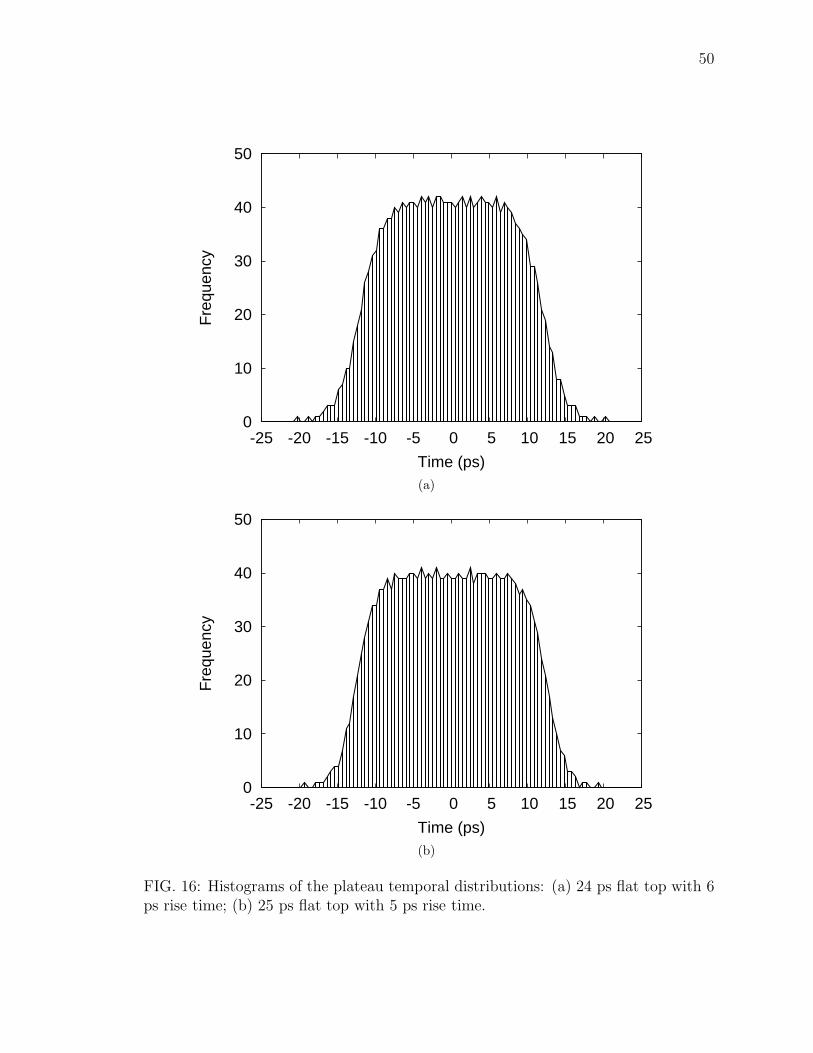
50

0

10

20

30

40

50

-25 -20 -15 -10 -5 0 5 10 15 20 25

Fre

quen

cy

Time (ps)(a)

0

10

20

30

40

50

-25 -20 -15 -10 -5 0 5 10 15 20 25

Fre

quen

cy

Time (ps)(b)

FIG. 16: Histograms of the plateau temporal distributions: (a) 24 ps flat top with 6ps rise time; (b) 25 ps flat top with 5 ps rise time.

51

-1

-0.5

0

0.5

1

-1 -0.5 0 0.5 1

p y (

keV

/c)

px (keV/c)

FIG. 17: Momentum distribution viewed in the px − py space.

-1

-0.5

0

0.5

1

0 0.2 0.4 0.6 0.8 1

p x (

keV

/c)

pz (keV/c)

(a)

-1

-0.5

0

0.5

1

0 0.2 0.4 0.6 0.8 1

p y (

keV

/c)

pz (keV/c)

(b)

FIG. 18: Momentum distribution viewed in the pz−px and pz−py spaces: (a) pz−px;(b) pz − py.

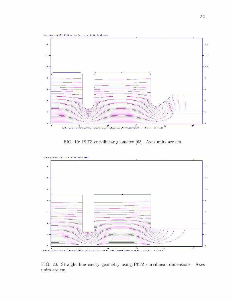
52

FIG. 19: PITZ curvilinear geometry [63]. Axes units are cm.

FIG. 20: Straight line cavity geometry using PITZ curvilinear dimensions. Axesunits are cm.

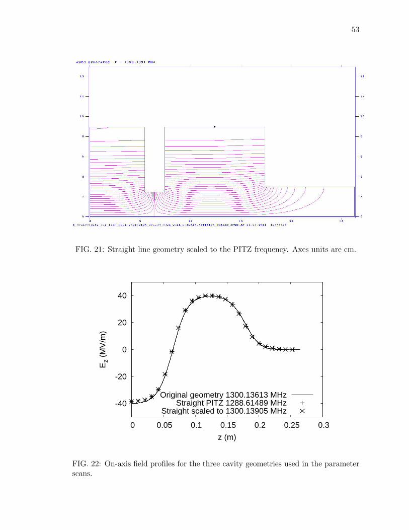
53

FIG. 21: Straight line geometry scaled to the PITZ frequency. Axes units are cm.

-40

-20

0

20

40

0 0.05 0.1 0.15 0.2 0.25 0.3

Ez

(MV

/m)

z (m)

Original geometry 1300.13613 MHzStraight PITZ 1288.61489 MHz

Straight scaled to 1300.13905 MHz

FIG. 22: On-axis field profiles for the three cavity geometries used in the parameterscans.

54

TABLE 4: Dimensions for the three study geometries

Dimension(cm)

PITZ curvilineargeometry [63]

Straight linegeometry withPITZdimensions

Straight linegeometry scaledto PITZfrequency

Frequency(MHz)

1300.1361 1288.6149 1300.1391

Cell 1 radius 9.0148 9.0148 8.9349

Cell 1 length 5.5 5.5 5.4513

Iris radius 2.5 (smallest) 2.5 2.4779

Iris length 2 2 1.9823

Cell 2 radius 9.0488 9.0488 8.9686

Cell 2 length 10 10 9.9114

Exit tubeand couplerradius

3 at exit of Cell 21.675 at tubeentrance

3 2.9734

Exit tubeand couplerlength

9 9 8.9203

Total length 26.5 26.5 26.2653

55

−10 −5 0 5 101400

1500

1600

1700

1800

1900

2000

Relative phase (degrees)

Ave

rage

num

ber

of a

ctiv

e pa

rtic

les

1 nC original geometry1 nC straight PITZ1 nC straight scaled800 pC original geometry800 pC straight PITZ800 pC straight scaled

FIG. 23: Average number of active particles at the end of each simulation for eachcombination of particle distribution and cavity geometry.

distribution performs better in terms of particle loss. Complementary to reporting

particle loss mechanisms, ASTRA also reports the number of active particles remain-

ing at the end of each simulation. As part of the parameter scans, the number of

active particles is recorded. Neither distribution is lossless. The loss pattern shows a

strong dependence on RF phase and a weak dependence on solenoid setting. This is

reflected in Figure 23 where the average number of active particles across all solenoid

settings is shown as a function of RF phase. For phases greater than -4◦, the sim-

ulations for the 800 pC distribution are lossless whereas the 1 nC distribution has

losses for most of the negative phases in the scan. This is notable because these are

the phases where RF guns typically run. The assumption that lossless transmission

simulation results are more reliable than those with losses justifies the choice to lower

the bunch charge from 1 nC to 800 pC in this research.

The parameter scans in Figures 24, 25, and 26 are consistent with each other and

previously published results. The PITZ work only provides a transverse emittance

contour plot for the parameter scan [7], and the transverse emittance contours here

56

match the PITZ result to the same level that [10] does. The actual transverse emit-

tance values are different for each bunch charge distribution, but more importantly,

across geometry descriptions for a given bunch charge distribution, the locations of

the minimum with respect to the solenoid and RF phase settings are in agreement.

As in [10], the beam size contour plots are provided to show that the location of the

minimum emittance in each parameter scan coincides with the minimum spot size

region as expected. These two observations confirm that the model is reasonable.

Considering the parameter scan results relative to the changes made in each set

guides approaches to use in the optimization to follow. The changes in the bunch

distribution do not significantly alter the pattern of the contours. Lowering the bunch

charge does lead to a direct improvement in the transverse emittance in all cases.

This suggests that reducing the bunch charge to obtain lossless, and therefore more

reliable, simulations in the optimization is acceptable, and that the net effect of doing

so lowers the transverse emittance. Also, whether the cavity geometry is made with

curved surfaces and rounded corners or straight lines and hard edge corners does

not affect the contours. Therefore, one might expect that straight line geometries,

which are intrinsically simpler to optimize, provide useful information about the

general optimization problem. In particular, the contour values for the straight line

geometry scaled to the PITZ frequency fall between the curved geometry and the

straight line cavity using PITZ dimensions. This suggests that the scaled geometry

is a good reference to use in the optimization.

Finally, because the PITZ RF gun has no longitudinal emittance requirement,

there is no reference set of longitudinal emittance contours for comparison. The lon-

gitudinal emittance is a candidate optimization objective function. The longitudinal

emittance contours are provided to establish a reference that can be used to interpret

the progress of an optimization using the longitudinal emittance.

4.2 FIELD MORPHING

The field morphing technique is used to find the minimum transverse emittance and

beam size under conditions similar to the parameter scan experiment. Primarily,

this exercise establishes that the optimization system works. It also validates the

proposed approach to optimize the RF gun field profile by varying it in response to

the beam dynamics. Third, it provides initial insights into what to expect from the

geometry optimization system when applied to a similar problem.

57

44

4.5

4.5

4.5

4.5

5

5

5

55

5.5

5.5

5.5

5.5

5.5

5.5

6

66

6

6

6

6.5

6.56.5

6.5

6.5

6.5

77

7

7

7

7

7.5

7.57.5

7.5

7.5

7.5

8

88

8

8

8

8.5

8.58.5

8.5

8.5

8.5

9

9

9

9

9

9

9.5

9.5

9.5

9.5

10

10

10

10.5

10.511

1111.5

1212.5

13

RF Phase (degrees)

Mai

n S

olen

oid

(Am

ps)

−10 −5 0 5 10285

290

295

300

305

(a)

2.5

2.5

2.5

3

3

3

3

3

3.5

3.5

3.5

3.5

3.5

3.5

44

4

4

4

4

4.5

4.5

4.5

4.5

4.5

5

5

5

5

5.5

5.5

5.5

6

6

6.5

6.5

7

77.5

8

RF Phase (degrees)

Mai

n S

olen

oid

(Am

ps)

−10 −5 0 5 10285

290

295

300

305

(b)

50

5050

6060

60

70

7070

8080

80

90

90

100

100

RF Phase (degrees)

Mai

n S

olen

oid

(Am

ps)

−10 −5 0 5 10285

290

295

300

305

(c)

3232.5

32.5

32.5

33

3333

33.5

33.5

33.5

3434

34

34

34.5

34.5

34.5

34.5

35

35

35

35.5

35.5

35.5

3636

36

36

36.5

36.5

3737

37.5

38

RF Phase (degrees)

Mai

n S

olen

oid

(Am

ps)

−10 −5 0 5 10285

290

295

300

305

(d)0.3

0.3

0.30.3 0.4

0.4

0.4

0.4 0.4

0.4

0.50.5

0.5

0.5

0.50.5

0.5

0.60.6

0.6

0.60.6

0.6

0.7

0.70.7

0.7

0.80.8

0.8

0.8

0.90.9

0.9

0.9

11

1

1

1.11.1

1.11.2

1.21.2

1.31.3

1.31.4

1.41.4

1.51.5

1.51.6 1.6

1.6

1.7

1.71.81.9

2

RF Phase (degrees)

Mai

n S

olen

oid

(Am

ps)

−10 −5 0 5 10285

290

295

300

305

(e)

0.2 0.2

0.20.20.3

0.3 0.3

0.3

0.30.30.3

0.4

0.4 0.4

0.4

0.4 0.40.40.5

0.5 0.5

0.5

0.5 0.5

0.5

0.6

0.6

0.6 0.6

0.6

0.70.7 0.7

0.7

0.80.8 0.8

0.90.9 0.91

1 1

1

1.11.1 1.1

1.21.2 1.2

1.31.3 1.3

1.41.4 1.41.5 1.5

1.6 1.61.7

RF Phase (degrees)

Mai

n S

olen

oid

(Am

ps)

−10 −5 0 5 10285

290

295

300

305

(f)

FIG. 24: Parameter scan results for the PITZ curvilinear geometry: (a) normalizedtransverse emittance for 1 nC; (b) normalized transverse emittance for 800 pC; (c)normalized longitudinal emittance for 1 nC; (d) normalized longitudinal emittancefor 800 pC; (e) beam size for 1 nC; (f) beam size for 800 pC.

58

55

5

5.5

5.5

5.5

5.56

6

6

6

6

6.5

6.5

6.5

6.5

6.5

6.5

7

7

7

7

7

7

7.5

7.5

7.5 7.57.5

7.5

8

8

8

8

8

8

8

8.5

8.5

8.5

8.58.5

8.5

9

9

9

9

9

9

9.5

9.5

9.5

9.5

9.5

10

10

10

10

10.5

10.5

10.5

11 11

11

11.5

11.5

11.5

12

12

12

12.5

12.5

13

1313.5

1414.5

15

RF Phase (degrees)

Mai

n S

olen

oid

(Am

ps)

−10 −5 0 5 10285

290

295

300

305

(a)

2.5

2.5

2.5

3

3

3

3

33.5

3.5

3.5

3.5

3.5

3.5

44

4

4

4

44.5

4.5

4.5

4.5

4.5

4.5

55

5

5

5

5

5.5

5.5

5.5

5.5

5.5

66

6

6

6

6.5 6.5

6.5

7 7

7

7.5 7.5

7.5

8

88.5

9

RF Phase (degrees)

Mai

n S

olen

oid

(Am

ps)

−10 −5 0 5 10285

290

295

300

305

(b)

5050

50

60

6060

7070

70

80

8080

90

90

90

90

100

100

100

100

RF Phase (degrees)

Mai

n S

olen

oid

(Am

ps)

−10 −5 0 5 10285

290

295

300

305

(c)

36

36

36

4040

4044

4444

4848

RF Phase (degrees)

Mai

n S

olen

oid

(Am

ps)

−10 −5 0 5 10285

290

295

300

305

(d)

0.3

0.3

0.4

0.4

0.4 0.5

0.50.5

0.50.6

0.60.6

0.6

0.70.7

0.7

0.7

0.80.8

0.8

0.8

0.90.9

0.9

0.9

11

1

1

1.11.1

1.1

1.1

1.21.2

1.2

1.2

1.31.3

1.3

1.3

1.41.4

1.4

1.4

1.51.5

1.5

1.5

1.61.6

1.6

1.6

1.71.7

1.7

1.7

1.81.8

1.8

1.8

1.91.9

1.9

1.9

22

2

2.1

2.1

2.22.32.42.5

RF Phase (degrees)

Mai

n S

olen

oid

(Am

ps)

−10 −5 0 5 10285

290

295

300

305

(e)

0.2 0.2

0.20.2

0.3

0.3 0.3

0.3

0.3

0.4

0.4 0.4

0.4

0.5

0.5 0.5

0.5

0.6

0.6 0.6

0.6

0.70.7 0.7

0.7

0.80.8 0.80.90.9 0.911 1

1

1.11.1 1.11.21.2 1.21.31.3 1.31.41.4 1.41.51.5 1.51.61.6 1.61.71.7 1.7

1.8 1.81.8

1.9 1.92

22.1

RF Phase (degrees)

Mai

n S

olen

oid

(Am

ps)

−10 −5 0 5 10285

290

295

300

305

(f)

FIG. 25: Parameter scan results for the straight line geometry: (a) normalized trans-verse emittance for 1 nC; (b) normalized transverse emittance for 800 pC; (c) nor-malized longitudinal emittance for 1 nC; (d) normalized longitudinal emittance for800 pC; (e) beam size for 1 nC; (f) beam size for 800 pC.

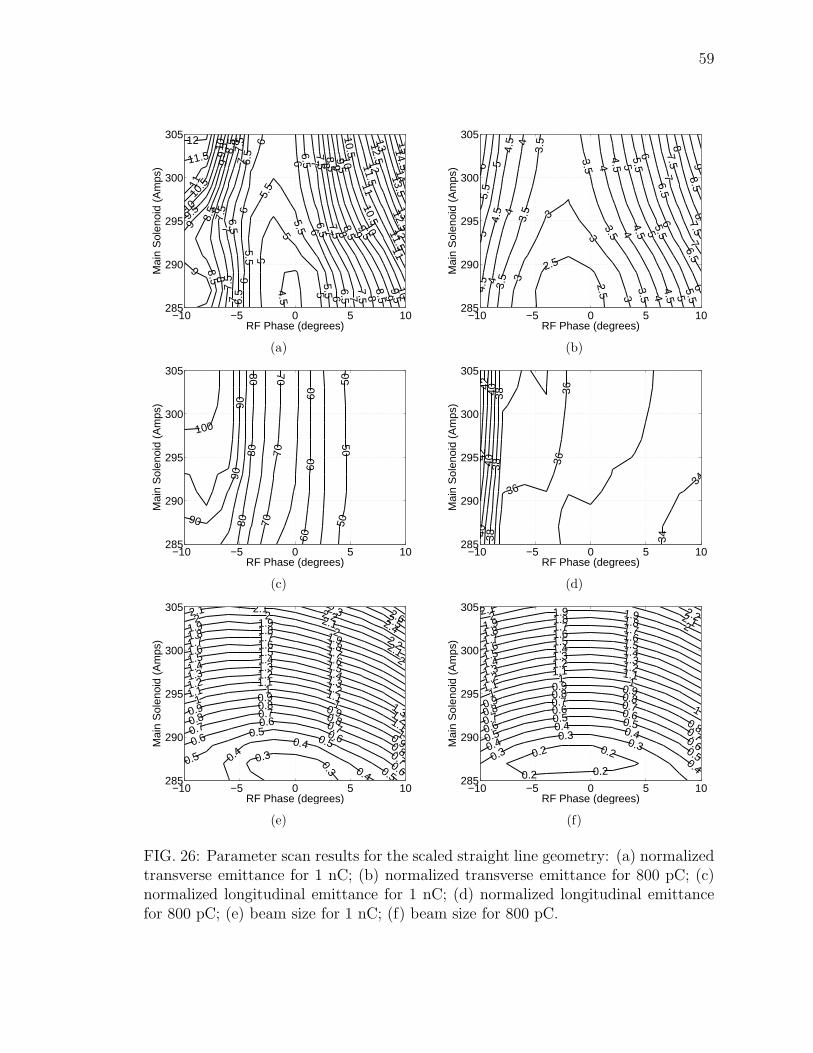
59

4.5

5

5

5

5.5

5.5

5.5

5.5

66

6

6

6

6

6.5

6.5

6.5

6.56.5

6.5

7

7

7

77

77.5

7.5

7.5

7.57.5

7.5

8

8

8

8

8

8

8.5

8.5

8.5

8.58.5

8.5

9

9

9

9

9

9

9.5

9.5

9.5

9.5

9.5

1010

10

10

10

10.5

10.5

10.5

11 11

11

11.5 11.5

11.5

12

12

12

12.5

12.5

13

1313.5

1414.5

15

RF Phase (degrees)

Mai

n S

olen

oid

(Am

ps)

−10 −5 0 5 10285

290

295

300

305

(a)

2.5

2.5

3

33

3

3.5

3.5

3.5

3.5

3.5

3.5

4

44

4

4

4

4.5

4.5

4.5

4.5

4.5

4.5

55

5

5

5

5.5

5.5

5.5

5.5

6

6

6

6

6.5

6.5

7

7

7.5

7.5

8

88.5

9

RF Phase (degrees)

Mai

n S

olen

oid

(Am

ps)

−10 −5 0 5 10285

290

295

300

305

(b)50

50

50

6060

60

7070

70

8080

80

9090

90

100

RF Phase (degrees)

Mai

n S

olen

oid

(Am

ps)

−10 −5 0 5 10285

290

295

300

305

(c)

34

3436

363638

3838

4040

4042

42

RF Phase (degrees)

Mai

n S

olen

oid

(Am

ps)

−10 −5 0 5 10285

290

295

300

305

(d)

0.3 0.3

0.40.4

0.4 0.5

0.50.5

0.50.6

0.60.6

0.6

0.70.7

0.7

0.7

0.80.8

0.8

0.8

0.90.9

0.9

0.9

11

1

1

1.11.1

1.1

1.1

1.21.2

1.2

1.2

1.31.3

1.3

1.3

1.41.4

1.41.5 1.5

1.51.6 1.6

1.6

1.7 1.71.7

1.8 1.81.8

1.9 1.91.9

2 22

2

2.1 2.12.1

2.1

2.2

2.2

2.32.42.52.6

RF Phase (degrees)

Mai

n S

olen

oid

(Am

ps)

−10 −5 0 5 10285

290

295

300

305

(e)

0.2 0.2

0.20.20.3

0.3

0.30.4

0.4 0.4

0.4

0.5

0.5 0.5

0.5

0.6

0.6 0.6

0.6

0.70.7 0.7

0.7

0.80.8 0.8

0.8

0.90.9 0.91

1 1

1

1.11.1 1.11.21.2 1.21.31.3 1.31.41.4 1.41.51.5 1.51.61.6 1.61.71.7 1.71.81.8 1.81.91.9 1.92

22.1

2.12.2

RF Phase (degrees)

Mai

n S

olen

oid

(Am

ps)

−10 −5 0 5 10285

290

295

300

305

(f)

FIG. 26: Parameter scan results for the scaled straight line geometry: (a) normalizedtransverse emittance for 1 nC; (b) normalized transverse emittance for 800 pC; (c)normalized longitudinal emittance for 1 nC; (d) normalized longitudinal emittancefor 800 pC; (e) beam size for 1 nC; (f) beam size for 800 pC.

60

The problem set up is the same as the RF phase and solenoid settings scan. The

layout of the beam line and the field profile for the main solenoid are carried forward.

The field profile for the RF gun though is no longer fixed since the optimization

generates it. The gradient is set to 40 MV/m, and the 800 pC particle distribution is

used. The optimization is configured to reject simulations with particle losses. The

cavity frequency used in the ASTRA simulations is the frequency of the generated

field, and the peak RF gradient is not rescaled to guarantee the peak gradient is fixed

in a relative location between the cells. The number of individuals per population is

96, and the maximum number of generations is 40.

The objectives of the optimization are to minimize the transverse emittance and

beam size. Technically, there are four objectives since ASTRA reports these quan-

tities for the horizontal and vertical planes [22]. The beam and the fields in this

problem are cylindrically symmetric, and that means the beam characteristics in the

horizontal and vertical planes match in the particle distribution at all points along

the beam line within statistical limits.

The main constraint is that min [fmorphing (z)] must be positive. This is to ensure

that fmorphing (z) does not introduce unwanted zero crossings. Additional constraints

are that the beam size and emittance must also be positive. These quantities by def-

inition are positive, so these constraints guard against unexpected invalid simulation

results.

The decision variables are the first seven pairs of Fourier coefficients of

fmorphing (z), a1 − a7 and b1 − b7; the relative RF phase of the gun; and the main

solenoid strength. The range for the main solenoid strength is the same as in the

parameter scan, and the relative RF phase range is opened up to ±15◦. The Fourier

coefficients are allowed to vary between 0 and 0.5. The units for the resulting field

profiles’ amplitudes are not specified since ASTRA normalizes the profiles so the

peak magnitude is 1 before scaling to the desired gradient setting in MV/m [22].

Figure 27 shows a sample of the non-dominated fronts from the 40 generations.

Recall that the non-dominated solutions in a population provide an estimate of the

Pareto-optimal front. They meet all of the constraints and have the best objective

values found so far. This figure shows that the estimate of the Pareto-optimal front is

progressively moving toward smaller and smaller beam sizes and emittances. Admit-

tedly, the final ranges of emittances and beam sizes are unacceptably large, so these

solutions are not attractive from an accelerator design standpoint. Also, the front

61

0

10

20

30

40

50

60

70

80

0 50 100 150 200 250

Bea

m s

ize

(mm

)

Transverse emittance (π mm mrad)

generation 1generation 5

generation 10generation 15generation 20generation 25generation 30generation 35generation 40

FIG. 27: Field morphing non-dominated individuals for several generations.

size is very small compared to the number of individuals in the population pointing

to a need for refinement of the optimization problem parameters. Still, the moving

front shows that the optimization system works and that the proposed approach is

viable.

Consider now the generated field profiles from the fronts of the first and last

generations in Figures 28 and 29. There is a similarity in the field profiles produced.

From the outset, the optimization processing shows a preference for unbalanced field

profiles to obtain small emittances. To date, cavities, whether for guns or accelerating

elements in linacs, are designed to have balanced or nearly balanced field profiles [65].

One way to characterize the balanced or unbalanced nature of the field profile is

to use field flatness [66], a percentage defined as

field flatness = 100|Epeak|max − |Epeak|min

1ncells

(

ncells∑

i=1

|Epeak|i)

where |Epeak|max and |Epeak|min are the maximum and minimum peak field amplitudes

across the cells, |Epeak|i is the peak of the i-th cell, and ncells is the number of cells.

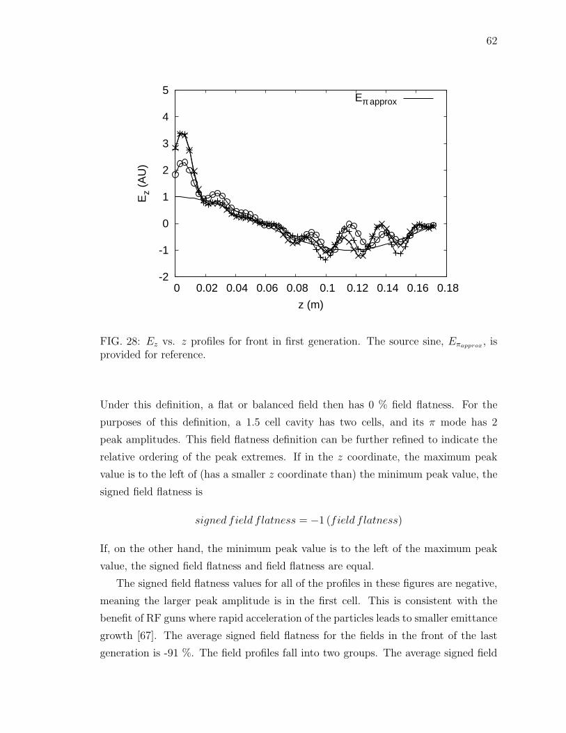
62

-2

-1

0

1

2

3

4

5

0 0.02 0.04 0.06 0.08 0.1 0.12 0.14 0.16 0.18

Ez

(AU

)

z (m)

Eπ approx

FIG. 28: Ez vs. z profiles for front in first generation. The source sine, Eπapprox, is

provided for reference.

Under this definition, a flat or balanced field then has 0 % field flatness. For the

purposes of this definition, a 1.5 cell cavity has two cells, and its π mode has 2

peak amplitudes. This field flatness definition can be further refined to indicate the

relative ordering of the peak extremes. If in the z coordinate, the maximum peak

value is to the left of (has a smaller z coordinate than) the minimum peak value, the

signed field flatness is

signed field flatness = −1 (field flatness)

If, on the other hand, the minimum peak value is to the left of the maximum peak

value, the signed field flatness and field flatness are equal.

The signed field flatness values for all of the profiles in these figures are negative,

meaning the larger peak amplitude is in the first cell. This is consistent with the

benefit of RF guns where rapid acceleration of the particles leads to smaller emittance

growth [67]. The average signed field flatness for the fields in the front of the last

generation is -91 %. The field profiles fall into two groups. The average signed field

63

-2

-1

0

1

2

3

4

5

0 0.02 0.04 0.06 0.08 0.1 0.12 0.14 0.16 0.18

Ez

(AU

)

z (m)

Eπ approx

FIG. 29: Representative Ez vs. z profiles for front in last generation. The sourcesine, Eπapprox

, is provided for reference.

flatness of the four smoother profiles is -56 %, and the average of the other two is -123

%. For the first group, the peak in the first cell is almost twice the peak amplitude

in the second cell, and in the latter case, the ratio is 4 to 1. These results are far

from nearly flat, in contrast to the PITZ case where the flatness is 10 % or less [68].

Figure 30 shows the components of the field morphing process for the field profile

in the last front that produces transverse emittance 34.733 π mm mrad and spot size

25.899 mm. The approximation to the π mode, Eπapprox(z), the morphing function,

fmorphing (z), and its an and bn terms are all shown. Summing the an and bn terms

with the offset 1 gives fmorphing (z). The curve for fmorphing (z) is well above zero as

required by the constraint. The resulting field profile, Ez (z), is also shown.

Initial attempts to optimize the transverse emittance for this problem using this

approach are described in [11]. The set up for those optimizations is slightly dif-

ferent from the one described here. For those, the problem definition included an

approximate description of the dimensions of the beam line enclosure. This defines

a set of apertures in the beam line that the beam must avoid to transport to the

64

-1

-0.5

0

0.5

1

1.5

2

2.5

0 0.02 0.04 0.06 0.08 0.1 0.12 0.14 0.16 0.18

Am

plitu

de (

AU

)

z (m)

Eπ approxEz

an fnbn fn

fmorphing

FIG. 30: Details for Ez vs. z profile that gives transverse emittance 34.733 π mmmrad and spot size 25.899 mm

end of the beam line. A related difference is that two particle loss mechanisms were

allowed, particles less than zmin and interception on apertures, but no attempt was

made to minimize the losses. Also, the 1.65 nC particle distribution from [10] was

reused. The RF phase and solenoid settings were fixed to the values corresponding

to the minimum emittance found in [10]. A final difference is the phases used for

the RF were not relative to the crest phase. Unfortunately, theses phases do not

translate between field maps even similar ones, and using these phases can lead to

invalid simulation results that otherwise might have been valid using relative phases.

Despite all of these differences, the optimizations point to unbalanced field profiles

as this more robust optimization configuration does.

From this field morphing exercise come three conclusions. The first is that the

proposal to change the field profile of the gun cavity as part of the beam dynamics

optimization works and makes sense to do. The second is that field morphing while

producing non-physical fields can yield compelling results that merit further study.

Lastly, specifically for RF gun design, it points to the possibility that gun designs

65

TABLE 5: Decision variables

Variable Units Lower bound Upper bound

relative RF phase degrees -10 15

main solenoid strength Tesla -0.180 -0.1

tube iris radius cm 2.4529 2.5029

tube iris length cm 1.9073 2.0073

cell 1 radius cm 8.9249 8.9449

cell 1 length cm 5.3763 5.4763

cell 2 radius cm 8.9586 8.9786

cell 2 length cm 9.88646 9.9864

with unbalanced field profiles lead to better emittances.

4.3 CAVITY GEOMETRY MORPHING

Finally, the cavity morphing optimization is applied to a variation of the parameter

scan experiment. In addition to minimizing the transverse emittance and beam

size, the longitudinal beam emittance is minimized. With this addition, the goal

of this optimization is to increase the brightness of the source. Recall from (2)

that brightness is inversely proportional to the product of the transverse emittances

and the longitudinal emittance. This is not part of the PITZ RF gun design or its

requirements. This is an exercise to see if the design can be improved to increase its

brightness.

The baseline cavity geometry for this optimization is the straight line cavity ge-

ometry scaled to the PITZ frequency. From the parameter scans presented, the

emittance product, εn,xεn,z, for the 800 pC bunch charge for this geometry is 76.24

π2 mm2 mrad keV. This calculation uses the point with the minimum transverse

emittance in the contour plot to determine this factor. The longitudinal emittance

decreases as the relative RF phase increases but at the expense of the transverse

emittance. The parameter scan indicates that the brightness can be improved only

marginally by adjusting the RF phase and main solenoid strength since the longi-

tudinal emittance does not change drastically over the entire parameter scan. If an

improvement is to be made, a different set of parameters needs to be considered.

66

TABLE 6: Linear relationship variables

Variable Tracked variable slope Offset

cell 1 neck width cell 1 length 1 0

cell 1 iris exit wall radius tube iris radius 1 0

cell 2 neck width cell 2 length 1 0

cell 2 iris entrance wall radius tube iris radius 1 0

In this optimization, the number of individuals is 96, and the maximum number

of generations is 10. As stated above, the objectives are the same as for the field

morphing optimization except for the addition of longitudinal emittance. The de-

cision variables and bounds are listed in Table 5. The upper bounds for the main

solenoid and RF phase are increased over the field morphing optimization settings.

According to [12], the frequency of the cavity is very sensitive to the cell radii, so

their bounds have been set to 0.02 cm windows around the scaled straight geometry

radii. The limits on the other dimensions are not so restrictive. This optimization

uses linear relationships to match some cavity dimensions to dimensions designated

as decision variables, and those are listed in Table 6.

The constraints related to beam characteristics are the same as for the field mor-

phing optimization. Similar to the field morphing optimization, there are constraints

related to the cavity morphing process. The frequency and field flatness of a cavity

depend on the cell radii of the cavity [12]. Changing the cell radii can drastically

change the resonance frequency of the geometry. Instead of tuning individual ge-

ometries to a desired frequency, constraints are used to guide the optimization to

cell dimensions that lead to desirable frequencies. In this case, the desired frequency

is 1300 MHz, and in the absence of equality constraints, two constraints are used

to place upper and lower bounds on the acceptable frequencies. These are 1300.5

MHz and 1299.5 MHz, respectively. Likewise, the range of acceptable signed field

flatnesses is controlled with two constraints. The bounds are ± 101 %. These limits

are chosen to allow for a large range of flatnesses while at the same time limiting

them to reasonable values. Even at 100 %, the difference in amplitudes between the

two cells is quite large.

Fronts are shown in Figures 31, 32, and 33. Bear in mind that the optimization

search space is nominally 3D, as opposed to 2D, in the field morphing case. This

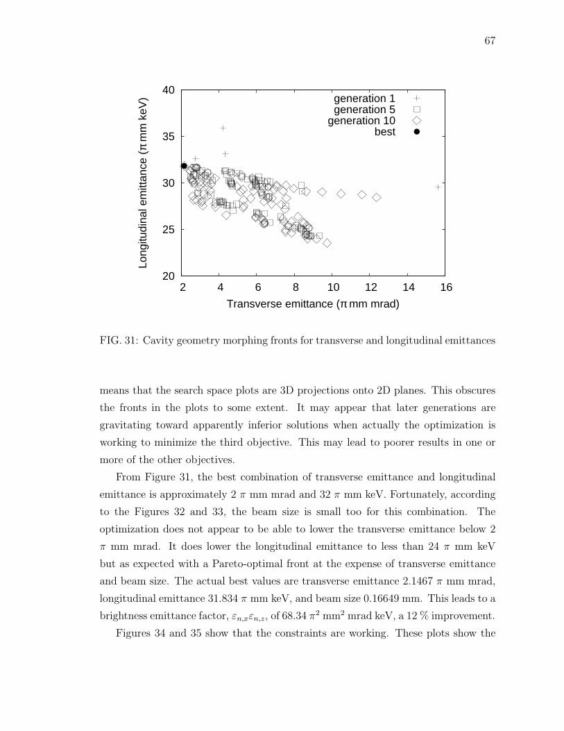
67

20

25

30

35

40

2 4 6 8 10 12 14 16

Long

itudi

nal e

mitt

ance

(π

mm

keV

)

Transverse emittance (π mm mrad)

generation 1generation 5

generation 10best

FIG. 31: Cavity geometry morphing fronts for transverse and longitudinal emittances

means that the search space plots are 3D projections onto 2D planes. This obscures

the fronts in the plots to some extent. It may appear that later generations are

gravitating toward apparently inferior solutions when actually the optimization is

working to minimize the third objective. This may lead to poorer results in one or

more of the other objectives.

From Figure 31, the best combination of transverse emittance and longitudinal

emittance is approximately 2 π mm mrad and 32 π mm keV. Fortunately, according

to the Figures 32 and 33, the beam size is small too for this combination. The

optimization does not appear to be able to lower the transverse emittance below 2

π mm mrad. It does lower the longitudinal emittance to less than 24 π mm keV

but as expected with a Pareto-optimal front at the expense of transverse emittance

and beam size. The actual best values are transverse emittance 2.1467 π mm mrad,

longitudinal emittance 31.834 π mm keV, and beam size 0.16649 mm. This leads to a

brightness emittance factor, εn,xεn,z, of 68.34 π2 mm2 mrad keV, a 12 % improvement.

Figures 34 and 35 show that the constraints are working. These plots show the

68

0

1

2

3

4

5

6

7

8

9

10

2 4 6 8 10 12 14 16

Bea

m s

ize

(mm

)

Transverse emittance (π mm mrad)

generation 1generation 5

generation 10best

FIG. 32: Cavity geometry morphing fronts for transverse emittance and beam size

0

1

2

3

4

5

6

7

8

9

10

20 25 30 35 40

Bea

m s

ize

(mm

)

Longitudinal emittance (π mm keV)

generation 1generation 5

generation 10best

FIG. 33: Cavity geometry morphing fronts for longitudinal emittance and beam size

69

TABLE 7: Geometry dimensions comparison

Dimension(cm)

Straight linegeometry scaled toPITZ frequency

High brightnessstraight linegeometry

Frequency (MHz) 1300.1391 1300.10216

Cell 1 radius 8.9349 8.93332

Cell 1 length 5.4513 5.38151

Iris radius 2.4779 2.48267

Iris length 1.9823 1.91288

Cell 2 radius 8.9686 8.97212

Cell 2 length 9.9114 9.97716

Exit tube andcoupler radius(not varied)

2.9734 2.9734

Exit tube andcoupler length(not varied)

8.9203 8.9203

Total length 26.2653 26.19185

first and last populations of the optimization and the members of the front, the non-

dominated individuals. Note that the first population is randomly generated, and

it is half the size of subsequent generations. The initial population consists of only

new individuals; there is no archive to augment its population as there is for later

generations. For both sets of constraints, in the first generation, there are individuals

outside of the constraint limits as expected for a randomly generated population, but

the individuals in the front are within the limits. By the last generation, almost all

individuals in the population lie within the constraint limits. Also, for the signed

field flatness, the front values tend to be negative even in the first generation. This

conclusion is consistent with the finding of the field morphing exercise. The signed

field flatness and frequency of the low brightness emittance factor case are -31.14

% and 1300.10216 MHz. The field profile for this case is shown in Figure 36. Its

geometry is shown in Figure 37 and its geometry parameters are listed in Table 7.

These results demonstrate that the cavity geometry morphing optimization works.

Further, they also show that this method can be used to improve an RF gun design

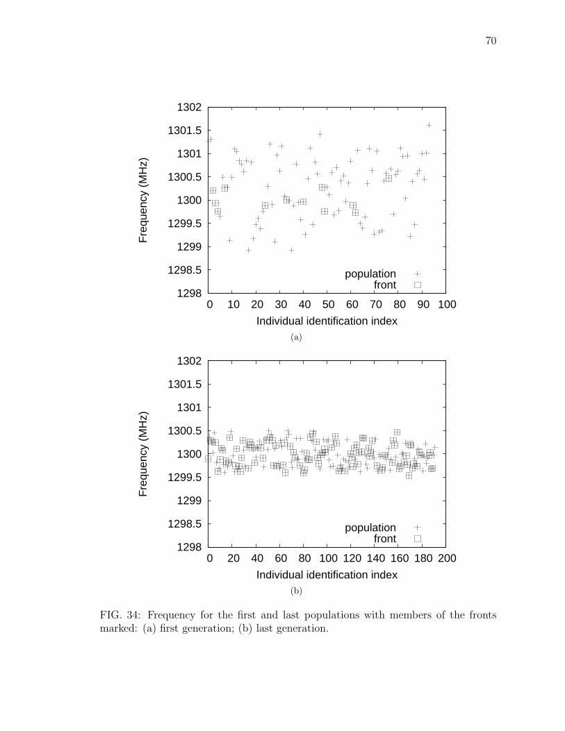
70

1298

1298.5

1299

1299.5

1300

1300.5

1301

1301.5

1302

0 10 20 30 40 50 60 70 80 90 100

Fre

quen

cy (

MH

z)

Individual identification index

populationfront

(a)

1298

1298.5

1299

1299.5

1300

1300.5

1301

1301.5

1302

0 20 40 60 80 100 120 140 160 180 200

Fre

quen

cy (

MH

z)

Individual identification index

populationfront

(b)

FIG. 34: Frequency for the first and last populations with members of the frontsmarked: (a) first generation; (b) last generation.

71

-100

-50

0

50

100

0 10 20 30 40 50 60 70 80 90 100

Sig

ned

Fie

ld F

latn

ess

(per

cent

)

Individual identification index

populationfront

(a)

-100

-50

0

50

100

0 20 40 60 80 100 120 140 160 180 200

Sig

ned

Fie

ld F

latn

ess

(per

cent

)

Individual identification index

populationfront

(b)

FIG. 35: Signed flatness for the first and last populations with members of the frontsmarked: (a) first generation; (b) last generation.

72

-40

-20

0

20

40

0 0.05 0.1 0.15 0.2 0.25 0.3

Ez

(MV

/m)

z (m)

Signed flatness -31.1 %

FIG. 36: Field profile for cavity geometry yielding transverse and longitudinal emit-tances 2.1467 π mm mrad and 31.834 π mm keV, respectively.

FIG. 37: Geometry for selected cavity geometry. Axes units are cm.

73

to produce a brighter beam. The previously mentioned field morphing method is

not consistent with any reasonable geometric boundary conditions. That method

suggests that skewing the field profile in the gun so that the peak amplitude is higher

in the first cell leads to better emittance. The cavity morphing method adheres to

boundary conditions by design, and the results from the cavity morphing method

reinforce the field morphing conclusion. An RF gun made with the reported geometry

will perform better from a brightness standpoint.

74

CHAPTER 5

SUMMARY AND CONCLUSION

RF guns are integral to the success of present and future accelerator based light

sources. It is important for the designs of these devices to be optimized to produce

the best quality beam as the requirement for brightness increases with each new light

source. Automation of the injector design process is useful because it enables the

injector designer to consider more designs more quickly. It also gives the designer the

ability to consider more design parameters to identify perhaps subtle or unorthodox

changes for improved performance. This conclusion summarizes the work performed

in this research and its findings in support of automating the injector design process

for RF guns. It also contains suggestions for improvements to the automated design

system to make its results more physically realizable and the system easier to use in

general. Finally, future research directions based on this work are listed.

This research has achieved two goals. The first is to develop a software tool that

allows injector designers to optimize the field profile of an RF gun and the injector

design in response to the performance characteristics of the beam dynamics. The

second is to apply the system to a state of the art RF gun to improve its performance.

This research builds on an injector design automation tool, APISA, based on

GAs. APISA was developed at Cornell and is in turn based on PISA from the ETH

in Switzerland. GAs use a population-based approach to search the objective space

for solutions to optimization problems with conflicting objectives and constraints.

GAs are especially well suited for injector optimization because they do not use or

require derivative information or analytical functional forms for the objectives or

constraints. It is often the case with injector performance that the interrelationship

between variables, objectives, and constraints is nonlinear or unknown. For that

reason, APISA uses the beam dynamics simulation program ASTRA to model the

injector and determine its performance characteristics. To extend APISA for use

with RF guns, this research adds the ability to modify the field profile of the RF gun

as part of the optimization. Previously, in APISA the field profiles were fixed.

Two methods for varying the field profile for the RF gun are provided. The first

method, called field morphing, ignores physical boundary conditions. It assumes a

functional form for the field profile to approximate the shape of a TM010 accelerating

75

π mode of a multi-cell RF cavity. This approximate field profile can be modified

then by a parameterized morphing function in response to the beam dynamics in the

system. Despite having possibly non-physical boundary conditions, optimizations

using this method can highlight desirable field characteristics to have in the field

produced by a physical cavity geometry.

The second more realistic method, called geometry morphing, addresses the

boundary condition deficiency of the first method. Because the field produced in

an RF cavity is solely a function of the geometry of the cavity, this approach uses

field profiles produced by an electromagnetic field solver for geometries of the RF

gun that have been modified by the optimization. The dimensions of the RF gun

cavity can be decision variables in the optimization that are changed in response to

the beam dynamics performance. For each modified geometry description, the opti-

mization system invokes the field solver to find the field profile to use in the beam

dynamics simulation. A present limitation of this system is that it uses straight

line approximations for the cavity geometries. As with the field morphing method,

this method can identify desirable field profile characteristics and the types of cavity

dimension changes needed to produce them.

Both methods have been applied to the state of the art PITZ 1.5 cell RF gun. In

both instances, the optimizations indicated that improved emittance performance is

possible with unbalanced field profiles. To date, RF gun designs have balanced field

profiles. This conclusion is in line with accepted practice where the field amplitude

peaks at the cathode in the half cell, but the results from the two methods go further

in saying that the peak field should be much higher at the cathode than it is in the

full cell. The cavity morphing method shows that an RF gun can be modified to

produce a brighter beam if designed to produce these significantly unbalanced field

profiles. It should be noted that no requirement on extracted beam energy is placed

on the optimizations.

There are several possible improvements for the system. They fall into three

categories. The first applies to the field morphing method. The second applies to

the geometry description, and the third applies to the optimization system itself.

Each will be described separately below.

Presently, the field morphing method can only morph the assumed form of the

π mode approximation. The method may be more useful and have more real world

applications if it morphed the field profile from a physical cavity. Additionally, the

76

field profile morphing method should be able to modify user provided field profiles

from a variety of cavity geometries. These changes would extend the utility of the

field morphing capability to other cavity geometries. Additionally, the peak field

rescaling capability for cavity morphing should be implemented for field morphing.

The geometry description developed for this research is very flexible and could

be extended to describe more detailed cavity geometries. For example, the geometry

description could be improved to include rounded corners and curved surfaces to

better reflect elliptical or re-entrant cavity geometries. Also, the addition of an

axisymmetric field coupler element would allow the coupler geometry to be changed

as part of the optimization and lead to better field representations in the coupler

region even if held fixed. The cavity geometry naturally defines a set of apertures, or

constrictions in the beam enclosure due to the irises in the cavity, and these apertures

can affect particle transmission. The aperture information is not available from the

existing system. It would be useful for the geometry description translation process to

produce the size and location of beam line apertures to include in the beam dynamics

simulation to account for this possible loss mechanism in the optimization. Finally,

the geometry description assumes that the cavity origin, (r = 0, z = 0), is located

at the base of the first (most upstream) vertical wall. While this is perfect for RF

guns where the center of the cathode is at (r = 0, z = 0), it is not suitable for other

cavity geometries where it is preferable to place the (r = 0, z = 0) location at the

geometric center of the cavity. Making the origin user configurable would allow the

same geometry description format to be used if the optimization system is extended

to modify other cavities in the beam line in addition to the RF gun or in lieu of it.

The optimization system is very flexible and powerful, but it can be improved.

First, the particle distribution creation system could be expanded. A useful addi-

tion to the existing particle distribution creation system is to allow the user to set

distribution parameters to default or fixed values without using decision variables.

The method used for setting defaults for the field morphing coefficients can serve as

a model. Another suggestion is to allow the optimization system to use the particle

distribution tool provided by the beam dynamics simulation program. Second, the

methods for setting variables in the optimization without affecting the decision vari-

able count should be expanded. It is now possible to establish a linear relationship

between a decision variable and another variable in the optimization. Consideration

should be given to nonlinear relationships. Third, the constraint system should be

77

expanded. It would be useful to be able to define constraints in terms of other vari-

ables in the system as opposed to fixed values. This would provide a way to order or

prioritize constraints. For example, it might be useful to ensure that one constraint

value is always less than another constraint value. Also, support for strict equality

and weak inequality constraints could be added. The present workaround to provide

an equality constraint is to define two bounding strict inequality constraints.

Two clear ways to improve the reliability of the system are outlined here. First,

the system would benefit from a better way to identify and deal with failed or stuck

program executions. Sometimes possible decision variable combinations are unfairly

marked unsuitable simply because the simulation failed to complete in the allotted

time. Increasing the time for each process is a work around but leads to unnecessarily

long optimization execution times. The addition of diagnostics to identify stuck

processes and the ability to optionally restart them would reduce the frequency of

this problem. Second, incorporating a Windows based program in a high performance

computing linux based environment presents its own challenges and contributes to the

fragility of the system. Finding linux based alternatives would reduce the complexity

of the system and increase its reliability.

In terms of usability, there are two recommendations to make the system easier

to use. The first relates to the data produced by the system. The system produces

a lot of very useful data, but there are few if any tools to organize and interpret

the results. A system that uses the configuration information in the system to auto-

matically aggregate and distill the data by generation, non-dominated front, decision

variables, constraints, and objectives would greatly help in interpreting the data and

bring to light the predictive nature of the evolution process. The second relates

to the fragmented nature of the optimization configuration. Because configuration

information is spread across several files in different locations, the initial set up of

an optimization is fairly error prone. Centralizing the configuration information can

address that problem.

Finally, this conclusion comes to the future directions for this research. Of a

more immediate nature, for the PITZ gun design, the effect of adding the bucking

solenoid to the system and varying the gradient of the gun can be studied. Also,

imposing more constraints and objectives based on cavity and field characteristics

may lead to additional cavity design recommendations. Using the existing cavity

geometry morphing system, it is possible to study the effect of inclining the walls of

78

the gun cell toward each other. Also, the effectiveness of re-entrant cavity shapes

for RF guns can also be considered with the existing system. The results of these

studies could be further strengthened with the addition of curved cavity geometry

shapes. Another outstanding question with respect to RF gun design is the optimal

frequency. Presently, the frequency of the gun used in an injector design is deter-

mined by existing cavity designs and the underlying RF infrastructure. Free of these

operational limitations, this optimization system can be used to see if there is a bet-

ter operational frequency. Lastly, the field morphing method can be used to find an

optimal number of cells for a gun design.

79

BIBLIOGRAPHY

[1] C. B. Wheeler, “Analysis of the planar field-emission diode,” Journal of Physics

D (Applied Physics), vol. 7, no. 2, pp. 267–279, 1974.

[2] B. M. Dunham, “Investigations of the physical properties of photoemission po-

larized electron sources for accelerator applications,” Ph.D. dissertation, Uni-

versity of Illinois at Urbana-Champaign, 1993.

[3] C. E. Mayes and G. H. Hoffstaetter, “Cornell energy recovery linac lattice and

layout,” in Proceedings of the 2010 International Particle Accelerator Confer-

ence, 2002, pp. 2356–2358.

[4] I. Bazarov, S. Belomestnykh, D. Bilderback, S. Gray, S. Gruner, Y. Li, M. Liepe,

H. Padamsee, V. Shemelin, C. Sinclair, R. Talman, M. Tigner, J. Welch,

G. Krafft, and L. Merminga, “Phase I energy recovery linac at Cornell Uni-

versity,” in Proceedings of the 2002 European Particle Accelerator Conference,

2002, pp. 644–646.

[5] M. Liepe, S. Belomestnykh, E. Chojnacki, Z. Conway, V. Medjidzade,

H. Padamsee, P. Quigley, J. Sears, V. Shemelin, and V. Veshcherevich, “The

Cornell high-current ERL injector cryomodule,” in Proceedings of the SRF2009,

2009, pp. 27–33.

[6] G. Neil, C. Behre, S. Benson, M. Bevins, G. Biallas, J. Boyce, J. Coleman,

L. Dillon-Townes, D. Douglas, H. Dylla, R. Evans, A. Grippo, D. Gruber,

J. Gubeli, D. Hardy, C. Hernandez-Garcia, K. Jordan, M. Kelley, L. Merminga,

J. Mammosser, W. Moore, N. Nishimori, E. Pozdeyev, J. Preble, R. Rimmer,

M. Shinn, T. Siggins, C. Tennant, R. Walker, G. Williams, and S. Zhang,

“The JLab high power ERL light source,” Nuclear Instruments and Methods

in Physics Research Section A: Accelerators, Spectrometers, Detectors and As-

sociated Equipment, vol. 557, no. 1, pp. 9 – 15, 2006.

[7] K. Abrahamyan, W. Ackermann, J. Bahr, I. Bohnet, J. P. Carneiro, R. Cee,

K. Flottmann, U. Gensch, H. J. Grabosch, J. H. Han, M. V. Hartrott,

E. Jaeschke, D. Kramer, M. Krasilnikov, D. Lipka, P. Michelato, V. Miltchev,

W. F. O. Muller, A. Oppelt, C. Pagani, B. Petrossyan, J. Robach, W. Sandner,

80

S. Schreiber, D. Sertore, S. Setzer, L. Staykov, F. Stephan, I. Tsakov, T. Wei-

land, and I. Will, “Characterization of the electron source at the photo injector

test facility at DESY Zeuthen,” Nuclear Instruments and Methods in Physics

Research A, vol. 528, no. 1-2, pp. 360–365, 2004.

[8] P. Emma, “First lasing of the LCLS x-ray fel at 1.5 A,” in Proceedings of the

2009 Particle Accelerator Conference, 2009, pp. 3115–3119.

[9] K. Tiedtke, A. Azima, N. von Bargen, L. Bittner, S. Bonfigt, S. Dusterer,

B. Faatz, U. Fruhling, M. Gensch, C. Gerth, N. Guerassimova, U. Hahn,

T. Hans, M. Hesse, K. Honkavaar, U. Jastrow, P. Juranic, S. Kapitzki, B. Keitel,

T. Kracht, M. Kuhlmann, W. B. Li, M. Martins, T. N. nez, E. Plonjes, H. Redlin,

E. L. Saldin, E. A. Schneidmiller, J. R. Schneider, S. Schreiber, N. Stojanovic,

F. Tavella, S. Toleikis, R. Treusch, H. Weigelt, M. Wellhofer, H. Wabnitz, M. V.

Yurkov, and J. Feldhaus, “The soft x-ray free-electron laser FLASH at DESY:

beamlines, diagnostics and end-stations,” New Journal of Physics, vol. 11, no. 2,

p. 023029, 2009.

[10] A. Hofler, P. Evtushenko, and M. Krasilnikov, “RF gun optimization study,” in

Proceedings of the 2007 Particle Accelerator Conference, 2007, pp. 1326–1328.

[11] A. Hofler, P. Evtushenko, and F. Marhauser, “Optimizing SRF gun cavity pro-

files in a genetic algorithm framework,” in Proceedings of the 2009 International

Computational Accelerator Physics Conference, 2009, pp. 296–299.

[12] A. Hofler and P. Evtushenko, “Optimizing RF gun cavity geometry within an

automated injector design system,” in Proceedings of the 2011 Particle Acceler-

ator Conference, 2011, pp. 805–807.

[13] I. V. Bazarov and C. K. Sinclair, “Multivariate optimization of a high bright-

ness DC gun photoinjector,” Physical Review Special Topics - Accelerators and

Beams, vol. 8, no. 3, p. 034202, 2005.

[14] L. Young and J. Billen, “The particle tracking code PARMELA,” in Proceedings

of the 2003 Particle Accelerator Conference, 2003, pp. 3521–3.

[15] J. H. Billen and L. M. Young, “POISSON/SUPERFISH on PC compatibles,”

in Proceedings of the 1993 Particle Accelerator Conference, 1993, pp. 790–792.

81

[16] J. Chen, W. Watson III, R. Edwards, and W. Mao, “Message passing for Linux

clusters with gigabit Ethernet mesh connections,” in Proceedings of the 19th

IEEE International Parallel and Distributed Processing Symposium, 2005, p. 8.

[17] K. Deb, Multi-objective optimization using evolutionary algorithms, ser. Wiley-

Interscience series in systems and optimization. Chichester: John Wiley and

Sons, 2001.

[18] M. Mitchell, An introduction to genetic algorithms, ser. Complex adaptive sys-

tems. Cambridge, Mass.: MIT Press, 1998.

[19] P. H. Winston, Artificial intelligence, 3rd ed. Reading, Mass.: Addison-Wesley

Pub. Co., 1992.

[20] C. Darwin, The origin of species by means of natural selection; or, The preserva-

tion of favored races in the struggle for life and the descent of man and selection

in relation to sex. New York: Modern library, 1936.

[21] S. Bleuler, M. Laumanns, L. Thiele, and E. Zitzler, “PISA - a platform and

programming language independent interface for search algorithms,” in Evolu-

tionary Multi-Criterion Optimization (EMO 2003), ser. Lecture notes in com-

puter science, C. Fonseca, P. J. Fleming, E. Zitzler, K. Deb, and L. Thiele, Eds.

Springer, 2003, pp. 494–508.

[22] K. Flottmann, “ASTRA: A Space Charge Tracking Algorithm,” http://www.

desy.de/∼mpyflo.

[23] B. M. Dunham, C. K. Sinclair, I. V. Bazarov, Y. Li, X. Liu, and K. W. Smolen-

ski, “Performance of a very high voltage photoemission electron gun for a high

brightness, high average current ERL injector,” in Proceedings of the 2007 Par-

ticle Accelerator Conference, 2007, pp. 1224–6.

[24] J. H. Billen and L. M. Young, “Poisson Superfish,” http://laacg1.lanl.gov/laacg/

services/serv codes.phtml.

[25] J. D. Lawson, The physics of charged-particle beams, 2nd ed., ser. The Inter-

national series of monographs on physics, no. 75. Oxford: Clarendon Press,

1988.

82

[26] A. W. Chao and M. Tigner, Handbook of Accelerator Physics and Engineering.

New Jersey: World Scientific, 1999.

[27] G. A. Krafft and J. Bisognano, “On using a superconducting linac to drive a

short wavelength FEL,” in Proceedings of the 1989 Particle Accelerator Confer-

ence, 1989, pp. 1256–8.

[28] P. Schmuser, M. Dohlus, and J. Rossbach, Ultraviolet and Soft X-Ray Free Elec-

tron Lasers: Introduction to Physical Principles, Experimental Results, Techno-

logical Challenges. Berlin: Springer, 2008.

[29] O. J. Luiten, “Beyond the RF photogun,” in The physics and applications of

high brightness electron beams: proceedings of the ICFA workshop, Chia Laguna,

Sardinia, 1-6 July 2002, J. Rosenzweig, G. A. Travish, and L. Serafini, Eds.,

2002, pp. 108–126.

[30] B. E. Carlsten, “New photoelectric injector design for the Los Alamos Na-

tional Laboratory XUV FEL accelerator,” Nuclear Instruments and Methods

in Physics Research A, vol. 285, no. 1-2, pp. 313–319, 1989.

[31] L. Serafini and J. B. Rosenzweig, “Envelope analysis of intense relativistic quasil-

aminar beams in RF photoinjectors: A theory of emittance compensation,”

Physical Review E, vol. 55, no. 6, p. 7565, 1997.

[32] A. Konak, D. W. Coit, and A. E. Smith, “Multi-objective optimization using ge-

netic algorithms: a tutorial,” Reliability Engineering and System Safety, vol. 91,

no. 9, pp. 992–1007, 2006.

[33] R. Marler and J. Arora, “Survey of multi-objective optimization methods for

engineering,” Structural and Multidisciplinary Optimization, vol. 26, pp. 369–

395, 2004.

[34] E. Zitzler and L. Thiele, “An evolutionary algorithm for multiobjective opti-

mization: the strength Pareto approach,” Computer Engineering and Networks

Laboratory (TIK), Swiss Federal Institute of Technology (ETH) Zurich, Glori-

astrasse 35, CH-8092 Zurich, Switzerland, Tech. Rep. 43, May 1998.

83

[35] E. Zitzler, “Evolutionary algorithms for multiobjective optimization: methods

and applications,” Ph.D. dissertation, Institut fur Technische Informatik und

Kommunikationsnetze, ETH Zurich, 1999.

[36] E. Zitzler, M. Laumanns, and L. Thiele, “SPEA2: Improving the Strength

Pareto Evolutionary Algorithm,” Computer Engineering and Networks Labora-

tory (TIK), Swiss Federal Institute of Technology (ETH) Zurich, Gloriastrasse

35, CH-8092 Zurich, Switzerland, Tech. Rep. 103, May 2001.

[37] ——, “SPEA2: improving the strength Pareto evolutionary algorithm for multi-

objective optimization,” in Evolutionary Methods for Design, Optimisation and

Control with Application to Industrial Problems (EUROGEN 2001), K. Gian-

nakoglou, D. Tsahalis, J. Periaux, K. Papailiou, and T. Fogarty, Eds., 2001, pp.

95–100.

[38] S. Bleuler, M. Laumanns, L. Thiele, and E. Zitzler, “PISA - a platform and

programming language independent interface for search algorithms,” Institut

fur Technische Informatik und Kommunikationsnetze, ETH Zurich, Tech. Rep.

154, October 2002.

[39] K. Deb and S. Agrawal, “A niched-penalty approach for constraint handling in

genetic algorithms,” in Artificial Neural Nets and Genetic Algorithms, 1999, pp.

235–243.

[40] K. Deb, “An efficient constraint handling method for genetic algorithms,” Com-

puter methods in applied mechanics and engineering, vol. 186, no. 2-4, pp. 311–

338, 2000.

[41] J. D. Knowles, L. Thiele, and E. Zitzler, “A tutorial on the performance assess-

ment of stochastic multiobjective optimizers,” Institut fur Technische Informatik

und Kommunikationsnetze, ETH Zurich, Tech. Rep. 214, 2005.

[42] M. M. Woolfson and G. J. Pert, An introduction to computer simulation. New

York: Oxford University Press, 1999.

[43] M. Frigo and S. G. Johnson, “The design and implementation of FFTW3,”

Proceedings of the IEEE, vol. 93, no. 2, pp. 216–231, 2005, special issue on

“Program Generation, Optimization, and Platform Adaptation”.

84

[44] M. Galassi, J. Davies, J. Theiler, B. Gough, G. Jungman, P. Alken, M. Booth,

and F. Rossi, GNU Scientific Library reference manual, 3rd ed. Network Theory

Limited, 2009.

[45] T. O’Haver, “Peak finding and measurement,” http://terpconnect.umd.edu/

∼toh/spectrum/PeakFindingandMeasurement.htm.

[46] Rosetta Code, “Polynomial regression,” http://www.rosettacode.org/wiki/

Polynomial regression.

[47] J. D. Jackson, Classical electrodynamics. New York: Wiley, 1999.

[48] J. Billen and L. M. Young, “Poisson Superfish,” Los Alamos National Labora-

tory, Los Alamos, New Mexico, Tech. Rep. LA-UR-96-1834, 2005.

[49] A. Julliard, “Wine,” http://www.winehq.org/.

[50] F. Krawczyk, private communication, 2008.

[51] X.org Foundation, “Xvfb,” http://www.x.org/releases/X11R7.6/doc/man/

man1/Xvfb.1.html.

[52] J. Kewisch, private communication, 2008.

[53] W. H. Press, B. P. Flannery, S. A. Teukolsky, and W. T. Vetterling, Numer-

ical recipes: the art of scientific computing, 3rd ed. New York: Cambridge

University Press, 2007.

[54] The Linux Foundation, “Linux,” http://www.linuxfoundation.org/.

[55] J. Swindle, “Wine-wiki,” http://wiki.jswindle.com/index.php/Main Page.

[56] IEEE Computer Society Task Force on Cluster Computing, “IEEE Task Force

on Cluster Computing,” http://www.ieeetfcc.org.

[57] R. C. Brower, C. E. DeTar, R. G. Edwards, D. J. Holmgren, R. D. Mawhinney,

W. W. III, and Y. Zhang, “National software infrastructure for lattice quantum

chromodynamics,” Journal of Physics: Conference Series, vol. 46, no. 1, p. 142,

2006.

85

[58] Adaptive Computing, “Maui cluster scheduler,” http://www.

adaptivecomputing.com/resources/docs/.

[59] Centos, “The Community ENTerprise Operating System,” http://www.centos.

org/.

[60] Thomas Jefferson National Accelerator Facility High Performance Computing,

“HPC Clusters,” http://wwwold.jlab.org/hpc.

[61] V. Miltchev, “Investigations on the transverse phase space at a photo injector

for minimized emittance,” Ph.D. dissertation, Humboldt-Universitat zu Berlin,

2006.

[62] L. Staykov and et. al., “Solenoid measurements at the Photo Injector Test Fa-

cility at DESY Zeuthen,” Photo Injector Test Facility at DESY Zeuthen, Tech.

Rep. PITZ-note, 2005.

[63] M. Krasilnikov, “Gun Benchmark Problem PITZ,” http://www.zeuthen.desy.

de/∼kras/PITZProblem.html/PITZbenchmark.html(defunct).

[64] R. T. Weidner and R. L. Sells, Elementary modern physics. Boston: Allyn and

Bacon, 1980.

[65] R. Boyce, D. H. Dowell, J. Hodgson, J. F. Schmerge, and N. Yu, “Design consid-

erations for the LCLS RF gun,” Stanford Linear Accelerator, Tech. Rep. LCLS

TN 04-4, April 2004.

[66] S. An and H. Wang, “Tuner effect on the field flatness of SNS superconduct-

ing RF cavity,” Thomas Jefferson National Accelerator Facility, Newport News,

Virginia and Spallation Neutron Source, Oak Ridge National Laboratory, Ten-

nessee, Tech. Rep. JLAB-TN-03-043 or SNS-NOTE-AP119, 2003.

[67] K. McDonald, “Design of the laser-driven RF electron gun for the BNL acceler-

ator test facility,” Electron Devices, IEEE Transactions on, vol. 35, no. 11, pp.

2052 –2059, Nov 1988.

[68] F. Stephan, C. H. Boulware, M. Krasilnikov, J. Bahr, G. Asova, A. Donat,

U. Gensch, H. J. Grabosch, M. Hanel, L. Hakobyan, H. Henschel, Y. Ivanisenko,

L. Jachmann, S. Khodyachykh, M. Khojoyan, W. Kohler, S. Korepanov,

86

G. Koss, A. Kretzschmann, H. Leich, H. Ludecke, A. Meissner, A. Oppelt,

B. Petrosyan, M. Pohl, S. Riemann, S. Rimjaem, M. Sachwitz, B. Schoneich,

T. Scholz, H. Schulze, J. Schultze, U. Schwendicke, A. Shapovalov, R. Spesyvt-

sev, L. Staykov, F. Tonisch, T. Walter, S. Weisse, R. Wenndorff, M. Winde, L. v.

Vu, H. Durr, T. Kamps, D. Richter, M. Sperling, R. Ovsyannikov, A. Vollmer,

J. Knobloch, E. Jaeschke, J. Boster, R. Brinkmann, S. Choroba, K. Flechsen-

har, K. Flottmann, W. Gerdau, V. Katalev, W. Koprek, S. Lederer, C. Martens,

P. Pucyk, S. Schreiber, S. Simrock, E. Vogel, V. Vogel, K. Rosbach, I. Bonev,

I. Tsakov, P. Michelato, L. Monaco, C. Pagani, D. Sertore, T. Garvey, I. Will,

I. Templin, W. Sandner, W. Ackermann, E. Arevalo, E. Gjonaj, W. F. O. Muller,

S. Schnepp, T. Weiland, F. Wolfheimer, J. Ronsch, and J. Rossbach, “Detailed

characterization of electron sources yielding first demonstration of European

X-ray Free-Electron Laser beam quality,” Physical Review Special Topics - Ac-

celerators and Beams, vol. 13, p. 020704, Feb 2010.

[69] C. K. Birdsall and A. B. Langdon, Plasma physics via computer simulation.

New York: McGraw-Hill, 1985.

[70] M. Reiser, Theory and design of charged particle beams, ser. Wiley series in beam

physics and accelerator technology. New York: Wiley, 1994.

[71] H. Wiedemann, Particle accelerator physics I basic principles and linear beam

dynamics. Berlin: Springer, 1999.

[72] K. Wille, The physics of particle accelerators an introduction. New York: Ox-

ford University Press, 2000.

[73] P. Lorrain and D. R. Corson, Electromagnetic fields and waves. New York:

W.H. Freeman, 1970.

[74] R. W. Hockney and J. W. Eastwood, Computer simulation using particles. Bris-

tol, England: A. Hilger, 1988.

[75] Computer Simulation Technology, “Microwave Studio,” http://www.cst.com/

Content/Products/MWS/Overview.aspx.

[76] Vector Fields Software, “Opera3d,” http://www.cobham.com/about-cobham/

aerospace-and-security/about-us/antenna-systems/kidlington.aspx.

87

[77] K. Flottmann, S. M. Lidia, and P. Piot, “Recent improvements to the ASTRA

particle tracking code,” in Proceedings of the 2003 Particle Accelerator Confer-

ence, 2003, pp. 3500–2.

[78] F. F. Chen, Introduction to plasma physics. New York: Plenum Press, 1976.

[79] C. W. Leemann, D. R. Douglas, and G. A. Krafft, “The Continuous Electron

Beam Accelerator Facility: CEBAF at the Jefferson Laboratory,” Annual Re-

view of Nuclear and Particle Science, vol. 51, no. 1, pp. 413–450, 2001.

[80] G. A. Krafft, private communication, 2008.

[81] W. E. Boyce and R. C. DiPrima, Elementary differential equations and boundary

value problems. New York: Wiley, 1977.

[82] T. Myint-U, Partial differential equations of mathematical physics. New York:

North Holland, 1980.

[83] Y. K. Batygin, “Particle-in-cell code BEAMPATH for beam dynamics simula-

tions in linear accelerators and beamlines,” Nuclear Instruments and Methods

in Physics Research A, vol. 539, no. 3, pp. 455–489, 2005.

[84] I. Rubinstein and L. Rubinstein, Partial differential equations in classical math-

ematical physics. Cambridge, England: Cambridge University Press, 1993.

[85] W. H. Press, B. P. Flannery, S. A. Teukolsky, and W. T. Vetterling, Numerical

recipes in C: the art of scientific computing. New York: Cambridge University

Press, 1988.

[86] R. L. Burden and J. D. Faires, Numerical analysis. Boston, Mass.: Prindle,

Weber and Schmidt, 1985.

[87] C. F. Gerald and P. O. Wheatley, Applied numerical analysis. Reading, Mass.:

Addison-Wesley Pub. Co., 1984.

[88] K. Halbach and R. F. Holsinger, “SUPERFISH - a computer program for eval-

uation of RF cavities with cylindrical symmetry,” Particle Accelerators, vol. 7,

no. 4, pp. 213–222, 1976.

88

[89] K. Deb, L. Thiele, M. Laumanns, and E. Zitzler, “Scalable multi-objective op-

timization test problems,” in Congress on Evolutionary Computation (CEC).

IEEE Press, 2002, pp. 825–830.

[90] ——, “Scalable test problems for evolutionary multi-objective optimization,” in

Evolutionary Multiobjective Optimization: Theoretical Advances and Applica-

tions, A. Abraham, R. Jain, and R. Goldberg, Eds. Springer, 2005, ch. 6, pp.

105–145.

[91] M. Kramer, C. Jarvis, and B. Terzic, “Locating optimal working point using an

evolutionary algorithm,” Thomas Jefferson National Accelerator Facility, New-

port News, Virginia, Tech. Rep., 2002.

[92] Adaptive Computing, “TORQUE resource manager,” http://www.

adaptivecomputing.com/resources/docs/.

[93] Sourceforge, “gnuplot,” http://www.gnuplot.info/.

[94] C. Faylor, C. Vinschen, and Red Hat, Inc., formerly Cygnus Solutions, “Cyg-

win,” http://www.cygwin.com/.

89

APPENDIX A

ASTRA OVERVIEW

A.1 INTRODUCTION

ASTRA is a beam dynamics code used to model injectors in the accelerator com-

munity. It is mainly used to simulate cylindrically symmetric systems but has 3D

capabilities [22]. This discussion describes the overall approach ASTRA uses for

modeling charged particle beams with space charge forces in accelerator beam lines.

All formulas and physical quantities in this discussion are expressed in SI (MKS)

units. The ASTRA suite of programs are listed with descriptions in Table 8.

A.2 PHYSICAL SYSTEM TO SIMULATE

ASTRA numerically describes the interactions between a collection of charged par-

ticles with electromagnetic fields that exist outside the bunch (external fields) and

those that originate from the close proximity of the charged particles in the bunch

(internal self fields). In general, the Newton-Lorentz force equation [69],

F = mdv

dt= q (E+ v ×B) (5)

describes how a charged particle responds to electric and magnetic fields. The elec-

tric and magnetic fields, both internal and external, can be found using Maxwell’s

equations [47],

∇ ·D = ρ, (6)

∇ ·B = 0, (7)

∇×H = J+∂D

∂ t, (8)

∇×E+∂B

∂ t= 0, (9)

where, for charged particles in vacuum [70], D = ε0E is the electric displacement,

ε0 is the electric permittivity of free space, E is the electric field, ρ is the charge

density, B = µ0H is the magnetic induction, µ0 is the magnetic permeability of

free space, H is the magnetic field, and J is the current density or displacement

current [47]. Because charged particle beams are typically accelerated to relativistic

90

TABLE 8: ASTRA programs and descriptions [22]

Program Description

generator Creates particle distributions from several differentprobability density functions based on user providedsettings. These particle distributions establish theinitial state of the particle bunch in terms of relativepositions in space, time, momentum, and charge.

Astra Beam dynamics simulation program. Its inputs areparticle distributions, beam line descriptions, andfield maps.

postpro Graphics program to plot phase space relatedquantities

lineplot Graphics program to plot calculated beamcharacteristics as a function of position along thebeam line or scanned quantities for parameter scans.

fieldplot Graphics program to plot field profiles for externaland space charge fields.

energies, ASTRA incorporates aspects of special relativity in its calculations. For

ease of discussion, the classical non-relativistic case is presented unless an idea or

concept from special relativity is used or needed explicitly.

External electromagnetic fields are used to control the path, expanse, and energy

of the particles [71,72]. External electric fields accelerate the particles when the field

is directed along the beam path. These fields can be fixed for DC guns or time varying

as produced in RF resonant cavities. The remaining external fields are magnetic and

constitute the beam transport system [71,72]. The beam transport system is mainly

responsible for containing the beam envelope which describes the extremes of all the

possible paths that the particles in the bunch can follow along the beam line [71,72].

The beam transport system consists of various types of magnets including solenoids,

dipoles, and quadrupoles [71,72]. Each magnet type serves a specific purpose in the

beam transport system. Dipoles bend the beam in one plane. Solenoids focus or

defocus the beam in all planes. Each solenoid’s action depends on its length relative

to the Larmor or cyclotron frequency [71, 73],

ωL =qB

m.

91

Quadrupoles act in two planes simultaneously focusing in one and defocusing in the

other.

The internal fields are the particle self fields that give rise to space charge forces

[70]. These forces push particles away from each other degrading the bunch and its

quality, and this is unacceptable in many accelerator applications. Gravity and the

earth’s field are part of the physical system of a particle accelerator, but they are not

explicitly accounted for in the simulation system. In general, the earth’s field is not

included in the model because the effect can be easily calculated and counterbalanced

in the beam transport system design. Also, gravity is neglected because its effect

is small compared to the forces that result from the electromagnetic field strengths

used in the accelerators [14].

A.3 PARTICLE BASED SIMULATION

A naıve approach to computing the trajectory of the particles in a charged particle

bunch is to compute each individual particle trajectory. To find a single particle

trajectory, the external and internal forces acting on the particle must be calcu-

lated. The self fields arise from the other particles in the bunch, and the interaction

between the one particle and the remaining particles must be calculated. This pro-

cess must then be repeated for each particle in the bunch. Because the number

of particles is so large, computing all pair-wise interactions in a charged particle

bunch is unreasonable. Instead, ASTRA uses macro-particles to describe the par-

ticle bunch [42, 69, 74]. Here, one simulation particle represents several particles in

the physical bunch, and the macro-particle’s properties reflect those of the individ-

ual particles it represents [42, 69, 74]. For charged particle beams, the collection of

macro-particles maintains the charge to mass ratio of the physical beam [42, 69].

Once the number of macro-particles to represent the system is chosen, the phys-

ical particle distribution is partitioned into a spatial grid [42, 69, 74]. Most particle

bunches in accelerators can be enclosed by a cylinder [25] that can be divided into

thin rings populated with point-like particles [22]. ASTRA uses this ring based par-

ticle mesh approach. The grids extend just beyond the boundary of the bunch [22]

and do not extend to the physical boundaries of the vacuum enclosure [69, 74].

Because the macro-particles are distributed across a grid and each macro-particle

represents several physical particles, the movement or redistribution of individual

92

particles as a result of the forces acting on them has to be accounted for in the macro-

particle model [42, 69]. ASTRA uses a ring based Particle in Cell (PIC) method

[42, 69, 74] with cubic spline interpolation to determine the charge density for each

grid cell for its cylindrically symmetric computations [22].

A.4 EXTERNAL FIELDS

ASTRA imports field calculation results computed by an electromagnetic field solver

code [22] such as Poisson Superfish [24], Microwave Studio [75], or Opera3d [76]. It

also uses internal numerical models for dipole and quadrupole elements [22]. When

using fields calculated outside the simulation code, the fields can be described with

three dimensional maps for which the system performs linear interpolations in three

dimensions to find the necessary field values at a particle’s location [77]. For cylin-

drically symmetric systems only the electric or magnetic field amplitudes along the

center axis, Ez (z, r = 0) or Bz (z, r = 0), are required [22]. In this case, the other

electric and magnetic field components for the RF cavity electric fields can be found

using a subset of Maxwell’s equations [77],

∇ · E = 0,

∇×B =1

c2dE

dt.

A similar technique can be used for the magnetic fields for the solenoids by solving

∇×B = 0 since J = 0 at r = 0 (which is outside the area occupied by the current

carrying magnet coils) [72]. For the electric fields that represent RF cavities, the time

variation of the electric field amplitude is modeled with a sinusoid with a phase shift

(cos (ω t+ ϕ)) [22]. ASTRA has analytic expressions with configurable parameters

for dipoles and quadrupoles [22].

A.5 INTERNAL FIELDS

The Debye length [70],

λD =

(

ε0kBT

q2n

)12

,

where kB is Boltzmann’s constant, T is the temperature of the collection of particles

in Kelvin, and n is the particle density, determines whether or not the self field or

space charge of the electrons is significant [69, 70, 78]. For electron beams, if λD is

smaller than the inter-particle spacing, ℓp, then an electron’s self field is “shielded”

93

from the other electrons in the system and collisions between particles have to be

considered [69,70,78]. Also as long as λD is much larger than ℓp, the self field forces

can be derived from smooth functions satisfying Poisson’s equation

∇2ϕ = − ρ

εo, (10)

and treated for other particles as external forces [70].

The size of λD relative to the bunch radius, rbunch, is still more significant [70]. If

λD is much smaller than or comparable to rbunch, each particle’s self field is significant

and must be included in the simulation process [70]. When λD is much smaller than

rbunch, the flow of the particles can be assumed to be laminar meaning the particle

paths do not cross [70]. When λD is comparable to rbunch, this last assumption is no

longer valid. The thermal velocity distribution of the particles must be considered,

and the self fields become nonlinear [70]. If λD is larger than rbunch, then self fields

can be ignored entirely [70]. For context, consider that, for Jefferson Lab’s polarized

source, λD is 12.5 µm and ℓp is 5.92 µm under the simplifying assumption that the

0.3 pC bunch is a 180 µm long cylinder with a 600 µm radius [79,80]. Clearly, λD is

much larger than ℓp and much less than rbunch, so the smooth self field and laminar

flow approximations apply. ASTRA is applicable to beams in this regime where

particle paths do not cross, space charge forces cannot be ignored, but can be found

using Poisson’s equation.

A.5.1 SIMPLIFYING SELF FIELD CALCULATIONS BY LORENTZ

TRANSFORMATION TO BUNCH REST FRAME

Because charged particle beams in particle accelerators move from non-relativistic to

relativistic energies in relatively short distances ranging from a few centimeters to

several meters, it is reasonable to calculate the space charge forces between particles

in a reference frame that moves with the beam (rest frame) instead of the laboratory

(lab) frame. The main advantage of this method is that evaluating the self fields be-

comes an electrostatic problem because the particles are at rest, so there is relatively

little current flow to generate magnetic fields [22]. Another is that the relativis-

tic form of the equations applies in the classical limit of Galilean relativity, so the

transition from non-relativistic to relativistic energies is handled automatically [64].

To see how the self field calculation problem is simplified, consider the example of

two Cartesian coordinate axes where one is fixed and the other, denoted with primes,

94

is attached to an electron moving at the speed of light in the positive x direction

from Jackson [47]. The two sets of axes are coincident at t = t′ = 0. The fields in

the rest frame of the electron, observed from a point that is a distance b in the y

direction from the origin of the lab frame are [47]

E ′

x = − qvt′

4πε0r′3 ,

E ′

y =qb

4πε0r′3 ,

E ′

z = B′

x = B′

y = B′

z = 0.

Lorentz transforming back to the lab frame using [73]

Ex = E ′

x,

Ey = γ [E ′

y + vB′

x] ,

Ez = γ [E ′

z − vB′

y] ,

Bx = B′

x,

By = γ[

B′

y −(

v/

c2)

E ′

z

]

,

Bz = γ[

B′

z +(

v/

c2)

E ′

y

]

,

γ =[

1− (v/c)2]−1/2

,

and [73]

x = γ [x′ + vt′] ,

y = y′,

z = z′,

t = γ[

t′ +(

v/

c2)

x′]

,

reveals the magnetic field that is associated with the moving charge [47, 73]

Ex = − γqvt

4πε0[

(γvt)2 + b2]3/2

,

Ey =γqb

4πε0[

(γvt)2 + b2]3/2

,

Ez = Bx = By = 0,

Bz = γv

c2qb

4πε0[

(γvt)2 + b2]3/2

=µ0

4π

γqbv[

(γvt)2 + b2]3/2

.

95

Because under relativity the electric and magnetic fields are not independent, only

one of the fields can be made to vanish in one of the two frames [47]. Even so, the

ability to eliminate one field in one frame greatly simplifies the self field calculation.

A problem with this method is that ASTRA transforms the particle positions and

velocities to the rest frame of the bunch using the average velocity of the bunch [22].

Not all of the particles in the bunch have this velocity; some particles move faster

and some slower. This means that the magnetic fields do not completely vanish in

this rest frame, and ASTRA is neglecting a possibly significant source of magnetic

fields.

A.5.2 SOLVING POISSON’S EQUATION

For electrostatic or nearly electrostatic (ρ varies slowly with time) problems,

∂B

∂ t= 0

(or approximately so). In this case, Maxwell’s equations, (6) to (9) reduce to

∇ · E =ρ

ε0, (11)

∇× E = 0. (12)

Now, a scalar potential, ϕ, satisfies (12) since

∇×∇ϕ = 0,

so for

E = −∇ϕ, (13)

(11) and (12) can be combined to form Poisson’s equation, (10) [47]. The process

for finding E is to find the potential, ϕ, from the charge density, ρ, using Poisson’s

equation and then find the electric field, E, using (13).

One standard method for solving partial differential equations is to use Fourier

series [81, 82]. Consider Poisson’s equation for an a× b rectangle in Cartesian coor-

dinates

− ρ

ε0=

∂2ϕ

∂x2+

∂2ϕ

∂y2(14)

with Dirichlet boundary conditions

ϕ (0, y) = ϕ (a, y) = ϕ (x, 0) = ϕ (x, b) = 0.

96

If ρ (x, y) and ϕ (x, y) are expressed as Fourier series [42, 83, 84]

ρ (x, y) =∞∑

m=1

∞∑

n=1

αmn sin(mπx

a

)

sin(nπy

b

)

,

ϕ (x, y) =

∞∑

m=1

∞∑

n=1

βmn sin(mπx

a

)

sin(nπy

b

)

,

where αmn and βmn are Fourier coefficients such that

αmn =

a∫

0

dξ

b∫

0

ρ (ξ, η) sinmπξ

asin

nπη

bdη

and βmn depends on αmn, then (14) gives

∞∑

m=1

∞∑

n=1

αmn sin(mπx

a

)

sin(nπy

b

)

= ε0

∞∑

m=1

∞∑

n=1

βmn

[

(mπ

a

)2

+(nπ

b

)2]

sin(mπx

a

)

sin(nπy

b

)

.

This leads to

βmn =αmn

ε0

[

(

mπa

)2+(

nπb

)2]

and, by (13), [42]

E = −{

i

∞∑

m=1

∞∑

n=1

βmn

mπ

acos(mπx

a

)

sin(nπy

b

)

+ j

∞∑

m=1

∞∑

n=1

βmn

nπ

bsin(mπx

a

)

cos(nπy

b

)

}

.

For cylindrically symmetric systems, the cylindrical form of Poisson’s equation

is used, and the a × b rectangle is a representative planar section of a cylinder with

radius a and length b [83]. The planar section is shown in Figure 38. The boundary

conditions for the cylindrically symmetric system are slightly different [83]. Along

r = a, the Dirichlet boundary condition still holds. Along r = 0, though, the

boundary condition is Neumann, meaning the derivative of the normal is specified

[81, 82], and for this case, it is zero. Finally, periodic boundary conditions are used

at z = 0 and z = b.

The numerical version for solving Poisson’s equation using Fourier series is essen-

tially the same except that it solves the finite difference form of Poisson’s equation

97

a

b

FIG. 38: Cylinder and planar section for Poisson’s equation.

and takes advantage of Fast Fourier Transform techniques to compute the series so-

lution for ρ from the charge distributed across the grid [42, 69, 83, 85]. The finite

difference form of (14) is [42, 69, 74, 86, 87]

−ρi,jε0

=ϕi+1,j − 2ϕi,j + ϕi−1,j

(∆x)2+

ϕi,j+1 − 2ϕi,j + ϕi,j−1

(∆y)2.

The finite difference method of expressing differential equations is based on Maclaurin

series expansions [86, 87]. The central difference based finite difference form of the

first derivative in one dimension is [42, 87]

f ′ (x) =f (x+ h)− f (x− h)

2h

where h is the interval size between uniformly spaced x values. This expression is

found from the difference of the two following Maclaurin series [42]

f (x+ h) = f (x) + hf ′ (x) +h2

2!f ′′ (x) +

h3

3!f ′′′ (x) +

h4

4!f (iv) (x) + . . . (15)

f (x− h) = f (x)− hf ′ (x) +h2

2!f ′′ (x)− h3

3!f ′′′ (x) +

h4

4!f (iv) (x) + . . . (16)

The trivial derivation proceeds as

f (x+ h)− f (x− h) = 2hf ′ (x) +2h3

3!f ′′′ (x) + . . .

f (x+ h)− f (x− h) = 2hf ′ (x) +O(

h3)

f (x+ h)− f (x− h)

2h= f ′ (x) +O

(

h2)

.

The likewise O (h2) second derivative used in Poisson’s equation is found in a similar

fashion by truncating the sums in (15) and (16) at the O (h4) term and solving for

f ′′ (x) [42].

98

A.6 SOLVING THE EQUATIONS: INTEGRATION

The final part of the simulation process after computing the individual fields and

forces for each particle is to compute the particle trajectory. This involves computing

the total force acting on each particle and then solving (5) numerically. The forces

are treated as a sum of the forces due to external fields and forces from fields derived

internally within the bunch [22, 70, 83]. ASTRA uses a fourth order Runge-Kutta

method with adaptive step size to integrate the Lorentz force equation [22]. The

fixed step Runge-Kutta method on which the adaptive step size version is based is

described here.

Systems modeled with first order differential equations such as (5) can be inte-

grated using the Runge-Kutta technique [42]. It is computationally quick, accurate,

and self-starting. It calculates all quantities for a given instance of time in a single

simulation time step [42]. The Runge-Kutta technique falls in the category of nu-

merical methods that find a direct solution to first order differential equations with

initial values (initial value problems) [42, 86, 87] of the form

dy

dx= f(x, y), (17)

y(xo) = yo. (18)

The general Runge-Kutta technique is an improvement on the Euler direct solu-

tion method [42, 86, 87]. The basis of the Euler method is that a point (x1, y1) on

a curve’s tangent at a nearby point (xo, yo) is a good approximation for the point

(x1, y1) on the curve [42]. In terms of a truncated Maclaurin series development

where h = x− xo, the Euler method is derived from [42, 86, 87]

y(x) ≈ y(xo) + hdy

dx

∣

∣

∣

∣

xo

= y(xo) + hy′(xo). (19)

By the system represented in (17) and (18), (19) becomes

y(x) ≈ y (xo) + hf (xo, y (xo)) = yo + hf(xo, yo)

or, more generally, [42, 86, 87]

xn+1 = xn + h,

yn+1 = yn + hf (xn, yn) .

99

The error for the Euler method is O (h) [42].

The Euler method can be improved with a better approximation for (x1, y1) de-

rived from the average of the slopes at (xo, yo) and (x1, y1) [42] or

y1 = yo +h

2(y′o + y′1) .

Here y′o = f (xo, yo) is the same as before, but y′1 depends on y1, an unknown. Using

the simple Euler method to give an estimate for y1 [42],

y1 = yo + hf (xo, yo) ,

leads to an estimate for y′1,

y′1 = f (x1, y1) .

Now, y1 is

y1 = yo +h

2{f (xo, yo) + f (x1, yo + hf (xo, yo))} .

The general scheme for the Euler predictor-corrector method with error O (h2) is [42]

xn+1 = xn + h,

yn+1 = yn +1

2(k1 + k2) ,

k1 = hf (xn, yn) ,

k2 = hf (xn+1, yn + k1) .

The Euler predictor-corrector method is an example of a second order Runge-Kutta

method [42]. The most commonly used fourth order Runge-Kutta scheme is [87]

yn+1 = yn +1

6(k1 + 2k2 + 2k3 + k4) ,

k1 = hf (xn, yn) ,

k2 = hf

(

xn +1

2h, yn +

1

2k1

)

,

k3 = hf

(

xn +1

2h, yn +

1

2k2

)

,

k4 = hf (xn + h, yn + k3) .

Fourth order Runge-Kutta methods have O (h4) and require four evaluations of

f(x, y), but the increased accuracy offsets the computational expense [42].

100

APPENDIX B

POISSON SUPERFISH

B.1 INTRODUCTION

Poisson Superfish is an electromagnetic field solver from Los Alamos National Labo-

ratory used in the accelerator community to calculate field information for magnets

and cylindrically symmetric RF cavity elements [48]. It is a collection of programs

that takes as input a geometry description of the structure of the magnet or the RF

element and other relevant information such as boundary condition treatment, cur-

rent flowing in magnet coil packs, and frequency for RF elements. From the geometry

description, a grid is generated, and the fields are calculated on the grid. With the

field and geometry information, various figures of merit and physical quantities of

interest to accelerator designers are calculated [48]. This appendix provides a listing

of the main Poisson Superfish programs in Table 9, and the methods used in Poisson

Superfish to compute the fields for RF cavities.

What follows is a reorganized and annotated restatement of the derivations and

information found in the theory summary of the document Poisson Superfish (LA-

UR-96-1834 Revised December 10, 2005). This describes the equations that Poisson

Superfish solves to calculate the field and the resonance frequency for a cavity. The

numerical techniques used to compute solutions to these equations are not discussed.

B.2 DERIVATION OF GENERALIZED HELMHOLTZ EQUATION

To find the field of a mode, Maxwell’s equations are simplified into two generalized

Helmholtz equations, one for transverse magnetic (TM) modes and the other for

transverse electric (TE) modes. Accelerator designers are typically more interested in

TM modes because these are accelerating modes, so Poisson Superfish solves the TM

mode version to find the cavity field. With an appropriate problem configuration,

though, Poisson Superfish can solve for the TE mode. This section outlines the

derivation of these generalized Helmholtz equations [48].

101

TABLE 9: Main Poisson Superfish programs [48]

Program Description

automesh Generates triangular mesh for problem geometrydescription

poisson Solves Poisson’s equation for magneto-staticproblems using successive over relaxation

pandira Solves Poisson’s equation for magneto-staticproblems using direct matrix inversion

fish Solves wave equation/Helmholtz equation for cavitystructures

sfo Calculates various physical quantities and figures ofmerit for poisson, pandira, and fish solutions

wsfplot Plots geometry, triangular mesh, and field contoursfor poisson, pandira, and fish solutions

sf7 Field interpolator

tablplot Plots output from sf7

autofish Runs automesh, fish, sfo, and wsfplot as oneprogram

Maxwell’s equations take the general form

∇× E = −∂B

∂t,

∇ ·D = ρ,

∇×H = J+∂D

∂t,

∇ ·B = 0,

where E is the electric field, B is the magnetic induction, D = εE is the electric

displacement, ε is the electric permittivity, ρ is the charge density, H = B/µ is

the magnetic field intensity, µ is the magnetic permeability, and J is the current

density [47]. Because an accelerating cavity is a vacuum or dielectric filled space

enclosed in a perfectly conducting surface, there is no charge density (ρ = 0) or

electric current density (J = 0) to create electric or magnetic fields in the cavity, so

Poisson Superfish recasts Maxwell’s equations in terms of two nonphysical quantities

that mirror the functionality of the charge and current densities. These are magnetic

102

charge density, σ, and magnetic current density, K. These new quantities then act

as excitation sources for electric and magnetic fields in the cavity. The resulting set

of equations that Poisson Superfish attempts to solve is

∇×E = −µ∂H

∂t+K, (20)

∇ · E = 0, (21)

∇×H = ε∂E

∂t, (22)

∇ ·H =σ

µ. (23)

Since σ and K do not exist in reality, they should not be present in the final solutions

to these equations. As the solutions approach resonance, K diminishes to zero as

required. Incidentally, these nonphysical quantities are the reason that a drive point

location is needed in the geometry description. Poisson Superfish needs to have a

source location for these quantities.

For three dimensional geometries such as RF cavities, Poisson Superfish takes

advantage of the generally cylindrically symmetric nature of these devices and re-

stricts itself to purely cylindrically symmetric problems. This implies that there is

no azimuthal, ϕ, dependence in the fields (i.e., ∂ (·)/∂ϕ = 0, E = E(r, z, t), and

B = B(r, z, t)). (20) to (23) take the following forms with component expressions

provided for reference. (20) becomes(

−∂Eϕ

∂z

)

r+

(

∂Er

∂z− ∂Ez

∂r

)

ϕ+1

r

(

∂ (rEϕ)

∂r

)

z

= −µ∂

∂t(Hrr+Hϕϕ+Hzz) + (Krr+Kϕϕ+Kzz) ,

and in component form

−∂Eϕ

∂z= −µ

∂Hr

∂t+Kr, (24)

∂Er

∂z− ∂Ez

∂r= −µ

∂Hϕ

∂t+Kϕ, (25)

1

r

(

∂ (rEϕ)

∂r

)

= −µ∂Hz

∂t+Kz. (26)

(21) is1

r

∂ (rEr)

∂r+

∂Ez

∂z= 0. (27)

(22) becomes(

−∂Hϕ

∂z

)

r+

(

∂Hr

∂z− ∂Hz

∂r

)

ϕ+1

r

(

∂ (rHϕ)

∂r

)

z = ε∂

∂t(Err+ Eϕϕ+ Ezz) ,

103

and is written in component form as

−∂Hϕ

∂z= ε

∂Er

∂t, (28)

∂Hr

∂z− ∂Hz

∂r= ε

∂Eϕ

∂t, (29)

1

r

(

∂ (rHϕ)

∂r

)

= ε∂Ez

∂t. (30)

Finally, (23) is1

r

∂ (rHr)

∂r+

∂Hz

∂z=

σ

µ. (31)

These equations are combined to form the two Helmholtz equations and an analogy

to the charge conservation equation. One Helmholtz equation in terms of Eϕ is used

to find TE modes, and the other in terms of Hϕ is for TM modes.

The first step in deriving the Eϕ equation is to combine (24), (26) and (29) to

form one equation in terms of Eϕ, Kr, and Kz

− ∂

∂r

[

1

r

∂ (rEϕ)

∂r

]

− ∂2Eϕ

∂z2+ µε

∂2Eϕ

∂t2=

∂Kr

∂z− ∂Kz

∂r. (32)

This equation comes about after taking the partial derivative of (24) with respect to

z

∂

∂z

(

−∂Eϕ

∂z

)

=∂

∂z

(

−µ∂Hr

∂t+Kr

)

∂

∂z

(

−∂Eϕ

∂z+ µ

∂Hr

∂t

)

=∂Kr

∂z

to get

−∂2Eϕ

∂z2+ µ

∂2Hr

∂z∂t=

∂Kr

∂z. (33)

Similarly, for (26) the partial derivative with respect to r results in

∂

∂r

(

1

r

∂ (rEϕ)

∂r

)

+ µ∂2Hz

∂r∂t=

∂Kz

∂r. (34)

Next, subtracting (34) from (33) leads to

−∂2Eϕ

∂z2+ µ

∂2Hr

∂z∂t− ∂

∂r

(

1

r

∂ (rEϕ)

∂r

)

− µ∂2Hz

∂r∂t=

∂Kr

∂z− ∂Kz

∂r.

Now, assuming separable and continuous functions (i.e., mixed partial derivatives

commute) and using (29) to rewrite the Hr and Hz terms as an Eϕ term, the result

is (32). Note that the right hand side of (32) is the ϕ component of ∇×K and can

104

be written as [∇×K]ϕ. Likewise, (25), (28) and (30) can be combined to form one

equation in terms of Hϕ and Kr

− ∂

∂r

[

1

r

∂ (rHϕ)

∂r

]

− ∂2Hϕ

∂z2+ µε

∂2Hϕ

∂t2= ε

∂Kϕ

∂t. (35)

These equations can be simplified to be purely spatially dependent. Assuming that

the time varying portion of K is oscillatory, K can be written as

K(r, z, t) = K(r, z) sinωt (36)

where ω = 2πf and f is the resonance frequency in Hertz. By the time dependence

of Eϕ in (32) and Hϕ in (35), then Eϕ and Hϕ are

Eϕ(r, z, t) = Eϕ(r, z) sinωt, (37)

Hϕ(r, z, t) = Hϕ(r, z) cosωt.

In order to use the identical code to solve for TE and TM modes, Hϕ is rescaled to

have the same units as Eϕ as follows

Hϕ(r, z, t) =

√

ε

µHϕ(r, z) cosωt. (38)

With the time behavior for Eϕ and Hϕ determined, the time dependence can be

removed from (32) and (35) since each term has a common sinωt factor after substi-

tuting in for Eϕ and Hϕ. Further, noting that for a cylindrically symmetric problem

in cylindrical coordinates

∇2f =1

r

∂

∂r

(

r∂f

∂r

)

+∂2f

∂z2

the Eϕ and Hϕ derivative terms with respect to r and z can be combined, and the

spatially dependent forms of (32) and (35) are

∇2Eϕ − 1

r2Eϕ + k2Eϕ = −

[

∇×K]

ϕ(39)

and

∇2Hϕ − 1

r2Hϕ + k2Hϕ = −k

√

ε

µKϕ (40)

where k =√µεω is the eigenvalue. (39) and (40) are general forms of the Helmholtz

equation. These are the equations that Poisson Superfish solves to find the fields.

105

Once solutions for Eϕ and Hϕ, and thereby Eϕ and Hϕ, are known, Hr, Hz, Er,

and Ez can be found by time integration of (24), (26), (28) and (30), respectively.

The general forms of these solutions are

Hr = −√

ε

µ

1

k

(

∂Eϕ

∂z+Kr

)

cosωt, (41)

Hz =

√

ε

µ

1

k

(

1

r

∂(

rEϕ

)

∂r−Kz

)

cosωt, (42)

Er = −1

k

∂Hϕ

∂zsinωt, (43)

Ez =1

kr

∂(

rHϕ

)

∂rsinωt. (44)

(43) and (44) satisfy (27). To satisfy (31) using (41) and (42), one develops a re-

striction for the magnetic charge and magnetic current densities akin to the electric

charge continuity equation for the standard set of Maxwell’s equations. This is the

analogous magnet charge conservation

∇ ·K sinωt+∂σ

∂t= 0. (45)

There is a sign difference though. Using (45) results in (31) giving −σ/µ instead of

σ/µ.

B.3 DERIVATION OF EQUATION FOR FINDING RESONANCE

Poisson Superfish uses a normalized quantity derived from the Poynting vector, S =

E×H, to find the resonance frequency of a mode [88]. The normalized quantity in

terms of the wave number, k = ω/c = 2πf/c where f is the cavity frequency, is

D(

k2)

= kc

∫

√

εµH ·Kdv

∫

εH2dv

. (46)

To see howD (k2) is useful in finding resonance, it is necessary to express it differently.

In the process of deriving an alternative expression, (46) is also derived [48].

First, integrate the Poynting vector following the standard prescription of taking

the divergence of S and then applying the Divergence theorem to find an expression

for the energy in the system. Using (20) and (22) from Maxwell’s equations recast

106

in terms of σ and K the divergence of S is

∇ · (E×H) = H · (∇× E)− E · (∇×H) ,

= H ·(

−µ∂H

∂t+K

)

− E ·(

ε∂E

∂t

)

,

= −µH · ∂H∂t

+H ·K− εE · ∂E∂t

,

= H ·K−(

µH · ∂H∂t

+ εE · ∂E∂t

)

,

= H ·K− 1

2

(

ε∂E2

∂t+ µ

∂H2

∂t

)

,

∇ · (E×H) = H ·K− 1

2

∂

∂t

(

εE2 + µH2)

.

Note for E and in like fashion for H that

∂

∂t

(

εE2

2

)

=ε

2

∂

∂t(E · E) = ε

22E · ∂E

∂t= εE · ∂E

∂t.

Integrating ∇ · (E×H) over the volume of the closed surface a gives

∫

∇ · (E×H) dv =

∫

H ·K− 1

2

∂

∂t

(

εE2 + µH2)

dv.

The Divergence theorem changes the volume integral on the left hand side into a

surface integral so∮

(E×H) · da =

∫

H ·Kdv − 1

2

∫

∂

∂t

(

εE2 + µH2)

dv.

Rearranging terms and moving the time derivative outside the integral gives∮

(E×H) · da+1

2

∂

∂t

∫

εE2 + µH2dv =

∫

H ·Kdv, (47)

the Poynting theorem for cavity fields. This equation describes how energy changes

inside the cavity and transfers in and out of it on the left side of the equation as a

result of the rate of work done on the cavity field by the magnetic current, K, on the

right side.

Because the cavity surface a is closed, all energy stays within surface a. This

means the first term in (47), describing energy entering and leaving the cavity through

the boundary surface a, is zero. This leaves

1

2

∂

∂t

∫

εE2 + µH2dv =

∫

H ·Kdv. (48)

107

The left side represents the time dependent change in energy in the fields in the

cavity. Assuming the previously stated spatial and time dependence for K, E, and

H, (36) to (38), gives

H ·K =

√

ε

µH ·K sinωt cosωt, (49)

E2 = E · E = E2sin2ωt, (50)

H2 = H ·H =ε

µH

2cos2ωt. (51)

Now, using (49) in the right hand side of (48) gives

∫

H ·Kdv = sinωt cosωt

∫ √

ε

µH ·Kdv.

Using (50) and (51) in the left hand side of (48) gives

1

2

∂

∂t

∫

εE2 + µH2dv = ω sinωt cosωt

∫

ε(

E2 −H

2)

dv.

Substituting these into (48) gives

∫ √

ε

µH ·Kdv = ω

∫

ε(

E2 −H

2)

dv.

This can be used to construct D (k2) and its alternative expression as follows

∫ √

ε

µH ·Kdv = ω

∫

ε(

E2 −H

2)

dv,

ω

∫

√

εµH ·Kdv

∫

εH2dv

= ω2

∫

ε(

E2 −H

2)

dv∫

εH2dv

,

kc

∫

√

εµH ·Kdv

∫

εH2dv

= (kc)2∫

εE2dv

∫

εH2dv

− (kc)2∫

εH2dv

∫

εH2dv

.

Note the left hand side in the last line is (46).

D(

k2)

= (kc)2∫

εE2dv

∫

εH2dv

− (kc)2.

From this formulation of D (k2), it is clear that on resonance, when the energy

stored in the electric and magnetic fields is equal, the ratio of integrals is one and,

108

therefore, D (k2) is zero. Finding the zeros of D (k2) is the first step in determining

the resonance frequency.

Unfortunately, not all zeros of D (k2) correspond to structure resonances. The

derivative of D (k2) with respect to (kc)2 is used to identify true resonances. This

derivative is

D′(

k2)

=D (k2)

2(kc)2− 1

2

∫

ε(

E2+H

2)

dv∫

εH2dv

. (52)

It evaluates to -1 when D (k2) is zero and the energy stored in the electric and

magnetic fields is equal, E = H, which is true on resonance. This means the second

step for finding the resonance frequency is to check thatD′ (k2) is -1 for the resonance

in question.

The derivative for D (k2) in (52) is found using the following steps. Rewriting

(46) as a product in terms of (kc)2

D(

k2)

=

√

(kc)2(∫ √

ε

µH ·Kdv

)(∫

εH2dv

)

−1

,

and applying the chain and product rules gives three terms. The first term in the

derivative is simply

∫

√

εµH ·Kdv

∫

εH2dv

d

d(kc)2

√

(kc)2 =1

2kc

∫

√

εµH ·Kdv

∫

εH2dv

=D (k2)

2(kc)2,

the first term of in (52). The general expression for the second term in the derivative

with ω = kc is

kc∫

εH2dv

d

d(kc)2

(∫ √

ε

µH ·Kdv

)

=kc

∫

εH2dv

∫ √

ε

µ

d

d(kc)2(

H ·K)

dv,

=ω

∫

εH2dv

∫ √

ε

µ

[

dH

d(kc)2·K+H · dK

d(kc)2

]

dv,

=ω

∫

εH2dv

∫ √

ε

µ

[

H′ ·K+H ·K′

]

dv.

If, as ω = kc nears resonance, K is changed slowly to keep H2constant, then H

′

and(

H2)

′

are zero, and

kc∫

εH2dv

d

d(kc)2

(∫ √

ε

µH ·Kdv

)

=ω

∫

εH2dv

∫ √

ε

µH ·K′

dv.

109

This simplifies to the second term in (52) as will be shown subsequently. The third

term is

kc

∫ √

ε

µH ·Kdv

d

d(kc)2

(∫

εH2dv

)

−1

= −kc

∫

√

εµH ·Kdv

(

∫

εH2dv)2

∫

d

d(kc)2

(

εH2)

dv = 0

because (H2)′

= 0. Combining all three terms gives

D′(

k2)

=D (k2)

2(kc)2+ ω

∫

√

εµH ·K′

dv

∫

εH2dv

. (53)

To convert (53) to the form in (52), use

∇ ·(

E×H′ −E

′ ×H)

= ∇ ·(

E×H′

)

−∇ ·(

E′ ×H

)

(54)

to derive an expression for the numerator of the second term. The left hand side

expands to

H′ ·(

∇× E)

− E ·(

∇×H′

)

−H ·(

∇× E′

)

+ E′ ·(

∇×H)

. (55)

Two of the curl terms are known from (20) and (22)

∇× E = K+√εµωH,

∇×H =√εµωE.

Their associated derivatives with respect to (kc)2 are

∇×E′

= K′

+√εµ

(

H

2ω+ ωH

′

)

,

∇×H′

=√εµ

(

E

2ω+ ωE

′

)

.

Using these in (54) and (55) gives

∇ ·(

E×H′ −E

′ ×H)

= H′ ·K−H ·K′ −

√εµ

2ω

(

E2+H

2)

.

Integrating and applying the Divergence theorem to the left hand side leads to∫

∇ ·(

E×H′ −E

′ ×H)

dv =

∮

(

E×H′ −E

′ ×H)

· da.

110

With an appropriate choice of boundary conditions, the right hand side vanishes,

leaving∫

∇ ·(

E×H′ − E

′ ×H)

dv = 0

∫

H′ ·K−H ·K′ −

√εµ

2ω

(

E2+H

2)

dv = 0.

Multiplying through by −√

ε/µ gives

∫ √

ε

µ

[

H ·K′ −H′ ·K+

√εµ

2ω

(

E2+H

2)

]

dv = 0

∫ √

ε

µ

(

H ·K′ −H′ ·K

)

dv =−1

2ω

∫

ε(

E2+H

2)

dv.

For H′

= 0, we have an expression for the numerator integral in (53)

∫ √

ε

µH ·K′

dv =−1

2ω

∫

ε(

E2+H

2)

dv

and substituting it in to (53) gives (52).

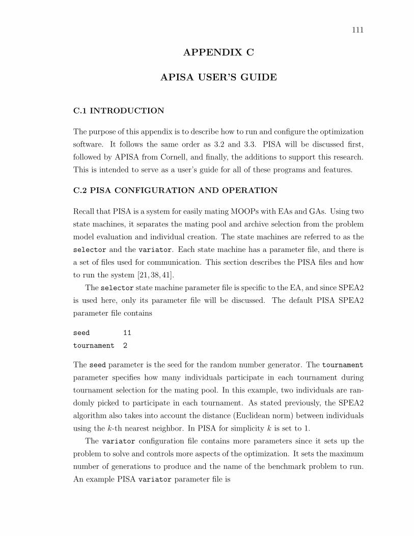
111

APPENDIX C

APISA USER’S GUIDE

C.1 INTRODUCTION

The purpose of this appendix is to describe how to run and configure the optimization

software. It follows the same order as 3.2 and 3.3. PISA will be discussed first,

followed by APISA from Cornell, and finally, the additions to support this research.

This is intended to serve as a user’s guide for all of these programs and features.

C.2 PISA CONFIGURATION AND OPERATION

Recall that PISA is a system for easily mating MOOPs with EAs and GAs. Using two

state machines, it separates the mating pool and archive selection from the problem

model evaluation and individual creation. The state machines are referred to as the

selector and the variator. Each state machine has a parameter file, and there is

a set of files used for communication. This section describes the PISA files and how

to run the system [21, 38, 41].

The selector state machine parameter file is specific to the EA, and since SPEA2

is used here, only its parameter file will be discussed. The default PISA SPEA2

parameter file contains

seed 11

tournament 2

The seed parameter is the seed for the random number generator. The tournament

parameter specifies how many individuals participate in each tournament during

tournament selection for the mating pool. In this example, two individuals are ran-

domly picked to participate in each tournament. As stated previously, the SPEA2

algorithm also takes into account the distance (Euclidean norm) between individuals

using the k-th nearest neighbor. In PISA for simplicity k is set to 1.

The variator configuration file contains more parameters since it sets up the

problem to solve and controls more aspects of the optimization. It sets the maximum

number of generations to produce and the name of the benchmark problem to run.

An example PISA variator parameter file is

112

problem KUR

seed 142

number_decision_variables 2

maxgen 100

outputfile dtlz_output.txt

individual_mutation_probability 1

individual_recombination_probability 1

variable_mutation_probability 1

variable_swap_probability 0.5

variable_recombination_probability 1

eta_mutation 20

eta_recombination 15

The problems defined in the variator are named according to the authors who

suggested them [89, 90]. The problem parameter sets the problem to optimize. The

seed parameter seeds the random number used in creating offspring individuals from

individuals in the mating pool. The number_decision_variables parameter sets

how many decision variables to use for the selected problem. The maximum number

of generations to produce is set with the maxgen parameter. The file named in

outputfile is where the results of the optimization are written. Specifically, this is

the information for the latest set of archive individuals identified by the selector

state machine. The information includes the decision variable settings and objective

values.

The remaining parameters in the variator configuration file pertain to gen-

erating offspring. The parameters, individual_recombination_probability and

individual_mutation_probability, are threshold probabilities for the recombi-

nation and mutations respectively. In order for the process to occur, a uniformly

generated number between 0 and 1 must be less than or equal to the threshold. In

this example, the threshold probabilities are both one, so both processes are allowed

for all individuals. The two recombination methods, uniform crossover and SBX,

also have threshold parameters. The variable_swap_probability parameter ap-

plies to uniform crossover while variable_recombination_probability applies to

SBX. For individuals that undergo recombination, for this example, uniform crossover

is applied to roughly 50 % of those individuals, and SBX is always applied. The

113

eta_recombination parameter is the ηSBX factor in the probability density func-

tion used in the SBX algorithm. Similarly, the variable_mutation_probability

and eta_mutation parameters govern the polynomial mutation process, and

eta_mutation is the ηpm parameter for its probability density function.

Six files are used for communication between the state machines. They share a

common prefix chosen by the user and are designated by suffixes, arc, cfg, ini, sel,

sta, and var. The cfg file is provided by the user and is used by both the selector

and variator. The remaining files are generated by the state machines.

The cfg file defines characteristics of the population, alpha, mu, lambda, and

dim. The default PISA cfg file contains

alpha 10

mu 10

lambda 10

dim 2

alpha is the number of individuals to generate for the initial population. mu is the

number of individuals to use as parents, and lambda is the number of children or

offspring to produce. For SPEA2, mu and lambda are equal. Lastly, dim is the number

of objectives.

The ini and var files are similar. They are created by the variator for use by

the selector. They both contain a list of the individual identifiers and objective

information. The ini file provides data about the initial population, and the var file

does the same for subsequent generations.

The arc and sel files are created by the selector. The sel file lists the individ-

ual identifiers for the mating pool, and the arc file lists the identifiers for the archive.

These files are used by the variator. The variator uses the arc file information

to prune individuals from the population.

Finally, the sta file is alternately written and read by both state machines. It is

used to keep track of the current state of the state machine processes. To facilitate

the easy interchange of variators and selectors, the PISA state machines have a

common simple structure of numbered states. The variator uses even numbered

states starting with zero while the selector uses odd numbered states. The sta

file is the semaphore file mentioned previously. The state machines poll this file to

coordinate processing. The active state machine, when it is finished, writes the next

successive state number to the file. For example, after completing initialization, state

114

0, the variator state machine writes a 1 to the sta file. This signals the selector

state machine to proceed to state 1.

To run the system, first the variator is started, and then the selector is started.

The argument list for the variator and the selector is the same. The first argument

is the program’s parameter file, followed by a tag name for the optimization. This tag

is the prefix name for the six communication files. The last argument is the polling

interval in seconds. Here is an example calling sequence for a computer running the

c shell on linux [54, 59]

variator variator_parameter.txt TAG 0.2 >& variator.out &

selector selector_parameter.txt TAG 0.2 >& selector.out &

This starts a variator process in the background using the configuration information

in variator_parameter.txt and TAGcfg. This process will check the TAGsta file

once every 0.2 seconds. Any standard or error output is captured in variator.out.

Similarly, the selector process is then started using selector_parameter.txt and

TAGcfg with its output and errors logged in selector.out. The general purpose

names variator and selector are used for the executables in this example, but the

processes can be named differently.

C.3 APISA SET UP

APISA [13] keeps the configuration system from PISA and builds on it. The changes

to the files used to communicate to the variator and selector processes are de-

scribed first. Next, the differences between the PISA and APISA variator and

selector specific parameter files are covered, and finally, descriptions of configura-

tion files added to the system complete the configuration file discussion.

Because the constraint value information is generated in the variator and used

in the selector, both state machines need to know the number of constraints in a

problem. For that reason, the number of constraints is added to the cfg file since both

programs read it. An example cfg file setting up a problem expecting 6 constraints

is

initial_population_size 8

parent_set_size 8

offspring_set_size 8

objectives 2

115

constraints 6

Note that in APISA the original variable names have been changed for readabil-

ity. alpha has been renamed initial_population_size. mu is the same as

parent_set_size. lambda is offspring_set_size. Finally, dim has become ob-

jectives.

In APISA, the ini and var files include values of the constraints in addition to

the objectives. The sel, arc, and sta files are unchanged. APISA adds an output

file to the common communication files to use for tracking the optimization. This

new file is a history file (his) and is not required for the operation of either state

machine to run. It is an information file created by the variator process. Since

it is configured in the variator parameter file, it is discussed subsequently in the

variator parameter file description.

The selector configuration file for SPEA2 has two additions, k_neighbor and

verbose as shown

seed 11

tournament 2

k_neighbor SQRT

verbose YES

The k_neighbor parameter makes it possible to set the k in the k-th nearest neighbor

routine. It can be set to SQRT to use the prescribed value in SPEA2 (√

N +N) or

to a positive integer. Debug information is written to the file spea2_diag.log when

verbose is set to YES. This information includes the generation number and number

of non-dominated individuals in the present archive.

The variator configuration file has a few additions. These are discussed next.

An example file is

problem ASTRA

astra_parameter_file /full/path/to/ASTRA/cfg/ast_param

seed 142

number_decision_variables 3

maxgen 2

force_selection NO

use_initial_decision_variables NO

use_initial_objectives NO

116

initial_data_file /full/path/to/restart/file/initial.txt

outputfile output.txt

individual_mutation_probability 1

individual_recombination_probability 1

variable_mutation_probability 1

variable_swap_probability 0.17

variable_recombination_probability 1

eta_mutation 20

eta_recombination 10

rotate_cw_objective12(deg) 0

append_last_generation YES

Although the parameter is not new, APISA adds a new problem type called ASTRA.

This setting directs APISA to use ASTRA for problem evaluations. The related

parameter addition is astra_parameter_file. The information in this tells the op-

timization where to find ASTRA–related set up information. The contents of this file

are discussed below. ASTRA input files, their formats, and details of running AS-

TRA simulations are not discussed. The interested reader is referred to the ASTRA

documentation [22].

Before proceeding with the discussion of the additions to the variator parame-

ters, some minor changes related to file output are described first. Because APISA

includes constraints, these values are included in the contents of the outputfile file.

Similar to the spea2_diag.log file, diagnostic information for the variator is al-

ways written to var_diag.log; it does not have a verbose switch. The information

written to the file includes the active nodes and the start time for each generation.

Three additions to the variator configuration file provide an optimization restart

mechanism: use_initial_decision_variables, use_initial_objectives, and

initial_data_file. When use_initial_decision_variables is set to YES,

APISA will read decision variable settings from the file named in the

initial_data_file file. This file contains one line per individual to add to

the population, and each line contains the values for the decision variables, the

objectives, and the constraints. If use_initial_decision_variables is set to

NO, all individuals in the initial population are generated randomly, and warm

restart is not used. The use_initial_objectives parameter is similar to the

use_initial_decision_variables parameter, but it determines whether or not

117

the objective and constraint information is used from the file. If set to YES, the data

in the file is used. If set to NO, the associated ASTRA simulations are run, and the

objective and constraints values are determined from the ASTRA output files.

The force_selection parameter directs APISA to use results from previous

generations that are still in the population (from the archive). This can reduce the

number of individuals that need to be generated but can cause unexpected results

[91]. This parameter should be used with care.

The rotate_cw_objective12(deg) parameter is specific to Cornell University’s

usage and is not generally useful. It assumes that the first two objectives for the

optimization are related by a rotation. The angle specified is used in the rotation

matrix to compute the rotated (or unrotated) values.

The append_last_generation parameter determines whether the his file men-

tioned previously in the communication file discussion contains a complete history

(YES) or not (NO) for the optimization. If a complete history is generated, APISA

appends the population information for each generation to the file. The population

contains the archive and the new individuals created. The information provided is

the same as in the outputfile, namely the values for the decision variables, ob-

jectives, and constraints. This allows one to see how the archive develops as the

optimization progresses. If the parameter is set to NO, only the results for the last

generation are provided as APISA overwrites the file each generation. In this case,

the contents of the his file are the same as outputfile.

The file named in astra_parameter_file contains mainly administrative in-

formation such as path names for ASTRA and APISA files and maximum time

allotments for job management. An example file contains

astra_binary /full/path/to/ASTRA/executable/Astra

astra_input_file /full/path/to/ASTRA/input/file/gun.in

available_nodes_file /full/path/to/computer/list/nodes_list

night_nodes_file NONE

max_jobs_node_file NONE

check_nodes YES

check_nodes_wait(sec) 30

maximum_time_per_job(min) 6000

maximum_jobs_per_node 1

keep_in_purgatory(sec) 60

118

niceness_level 0

use_unused_nodes_only NO

users_usage_threshold 25.0

system_usage_threshold 25.0

node_inactive_wait(min) 15.0

generate_distributions NO

append_results_file /full/path/for/debug/data/RESULTS

distribution_directory /full/path/for/new/distributions/dist

number_particles 1000

astra_output_names_file /full/path/to/ASTRA/out/data/ast_name

decision_variables_file /full/path/to/decision/cfg/decisions

objectives_file /full/path/to/objective/cfg/objectives

constraints_file /full/path/to/constraint/cfg/constraints

The file contents are described in terms of groups of related variables, and therefore

will be discussed out of order relative to the example.

Beyond a linux or unix like operating system, APISA makes no assumptions about

the file system or location of files. This makes APISA very configurable and means

the user has to specify several file locations. The first two variables in the ASTRA set

up file, astra_binary and astra_input_file, provide the location of the ASTRA

program executable and the ASTRA input file to use as a template for each ASTRA

run. For each individual, APISA makes a customized copy of the template file

reflecting the individual’s decision variable values to use as input to ASTRA. The

individual ASTRA input files use the base name of the template file, gun in this case,

followed by an individual identification number and a computer name. An example

individual ASTRA input file name is gun.000000008.computer1.in.

The next set of ASTRA variables is located in the lower half of the file. These

relate to the particle distribution. The generate_distributions variable indicates

whether APISA should generate a particle distribution for each individual (YES) or

use one particle distribution provided by the user for all individuals (NO). If the vari-

able is set to YES, APISA will generate particle distributions containing the number

of macro-particles specified with number_particles and put the files in the directory

named in distribution_directory. Each distribution file is named according to

its corresponding ASTRA input file but with a .dis file extension. For the example

input file above, its generated distribution file is gun.000000008.computer1.dis.

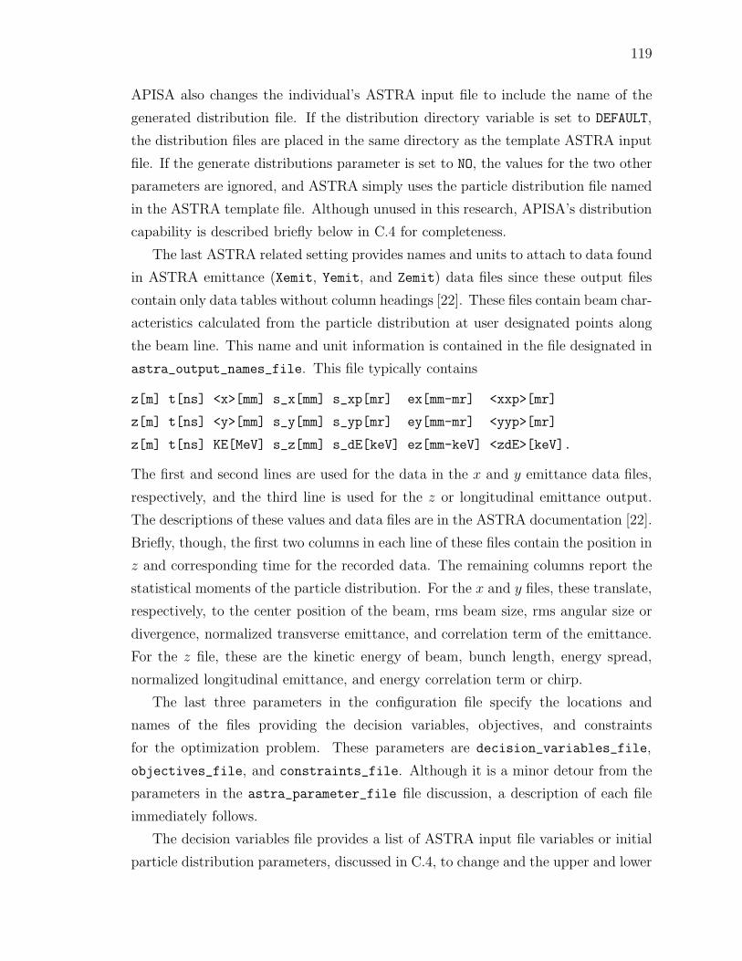
119

APISA also changes the individual’s ASTRA input file to include the name of the

generated distribution file. If the distribution directory variable is set to DEFAULT,

the distribution files are placed in the same directory as the template ASTRA input

file. If the generate distributions parameter is set to NO, the values for the two other

parameters are ignored, and ASTRA simply uses the particle distribution file named

in the ASTRA template file. Although unused in this research, APISA’s distribution

capability is described briefly below in C.4 for completeness.

The last ASTRA related setting provides names and units to attach to data found

in ASTRA emittance (Xemit, Yemit, and Zemit) data files since these output files

contain only data tables without column headings [22]. These files contain beam char-

acteristics calculated from the particle distribution at user designated points along

the beam line. This name and unit information is contained in the file designated in

astra_output_names_file. This file typically contains

z[m] t[ns] <x>[mm] s_x[mm] s_xp[mr] ex[mm-mr] <xxp>[mr]

z[m] t[ns] <y>[mm] s_y[mm] s_yp[mr] ey[mm-mr] <yyp>[mr]

z[m] t[ns] KE[MeV] s_z[mm] s_dE[keV] ez[mm-keV] <zdE>[keV].

The first and second lines are used for the data in the x and y emittance data files,

respectively, and the third line is used for the z or longitudinal emittance output.

The descriptions of these values and data files are in the ASTRA documentation [22].

Briefly, though, the first two columns in each line of these files contain the position in

z and corresponding time for the recorded data. The remaining columns report the

statistical moments of the particle distribution. For the x and y files, these translate,

respectively, to the center position of the beam, rms beam size, rms angular size or

divergence, normalized transverse emittance, and correlation term of the emittance.

For the z file, these are the kinetic energy of beam, bunch length, energy spread,

normalized longitudinal emittance, and energy correlation term or chirp.

The last three parameters in the configuration file specify the locations and

names of the files providing the decision variables, objectives, and constraints

for the optimization problem. These parameters are decision_variables_file,

objectives_file, and constraints_file. Although it is a minor detour from the

parameters in the astra_parameter_file file discussion, a description of each file

immediately follows.

The decision variables file provides a list of ASTRA input file variables or initial

particle distribution parameters, discussed in C.4, to change and the upper and lower

120

bounds for the generated values. An example decision variable file is

MaxB(1) VARY -0.179 -0.168

MaxB(2) VARY |-> MaxB(1) 0.5 1.0

MaxB(3) VARY |-> MaxB(1) 0 0

This three line example shows the two possible decision variable declarations. Each

line designates a different solenoid field amplitude variable in the ASTRA input

file to change. APISA uses the information in this file to generate values for these

variables within the specified ranges for each individual in each generation. The first

line indicates that the ASTRA input file variable MaxB(1) values are restricted to the

range of -0.179 and -0.168 Tesla. The second line directs APISA to generate an offset

for each individual between 0.5 and 1.0 Tesla and then sums it with that individual’s

MaxB(1) value to arrive at its value of MaxB(2). The third line generates the value

zero and sums it with the value of MaxB(1) to compute the value of MaxB(3). This

last line shows how to make two decision variables have the same value in Cornell’s

original version of APISA, and an alternative approach is presented in C.5.2. In this

example while MaxB(1) differs between individuals, for each individual, MaxB(3) and

MaxB(1) are always set to the same value.

The constraints file lists the ASTRA output and decision variables that are used as

constraints in the optimization. As stated earlier, the constraints are limited to strict

inequalities and are designated using the keywords GREATER_THAN and LESS_THAN.

Each line in the file contains an output variable name followed by an inequality

keyword and the upper or lower bound value. In the example below the horizontal

beam size (s_x) must be greater than 1.0 mm, and the vertical beam size (s_y) must

be less than 4.0 mm.

s_x GREATER_THAN 1.0

s_y LESS_THAN 4.0

The objectives file lists the objectives of the optimization, and because the system

is designed to optimize a multi-objective system, the file must contain at least two

objectives. An objective file entry contains an ASTRA output or decision variable

followed by the keyword MAXIMIZE or MINIMIZE, depending on the optimization goal

for the value. In this example the emittance in both the horizontal and vertical

planes must be minimized.

121

ex MINIMIZE

ey MINIMIZE

Returning to the parameters in the astra_parameter_file file discussion, the

remainder of the parameters in the ASTRA set up file either aid in debugging and

tracking the progress of the optimization or are used to manage APISA in a paral-

lel computing environment. The parallel computing controls are designed to allow

APISA to run in any linux environment where there is a shared file system. That flex-

ibility points to several configuration parameters and are discussed after the debug

and tracking variables.

append_results_file can be used to track the optimization progress. This is

different from the outputfile and his files described above. Its purpose is to create

a record of all the various output values from ASTRA or computed from ASTRA

results and the decision variable settings. The two previously discussed files provide

values for the decision variables, objectives, and constraints, a considerably smaller

set of values. If append_results_file is set to NONE, no file is created. If it is set

otherwise, its value is used as the name of the file to create. In the example above, the

created file is named RESULTS. After the first individual finishes processing, APISA

writes to the bottom of the specified file the time that the optimization started

along with the names of the decision and ASTRA output parameters. Then as

each individual (including the first) finishes processing, APISA appends the decision

variable and ASTRA output values to the file.

Another variable that can be used to monitor APISA intermediate results is

keep_in_purgatory(sec). APISA by default cleans up as it proceeds removing

generated files once they are no longer needed. This reduces file system clutter as

the process runs but can hamper debugging as ASTRA output files that a user may

want to inspect disappear very soon after the ASTRA simulation stops. Setting the

keep_in_purgatory(sec) parameter instructs APISA to wait the specified number

of seconds after the ASTRA simulation completes before removing the files. In this

example, APISA waits 60 seconds before removing files.

The discussion moves now to the parallel processing controls. These parameters

are repeated here

available_nodes_file

night_nodes_file

max_jobs_node_file

122

check_nodes

check_nodes_wait(sec)

maximum_time_per_job(min)

maximum_jobs_per_node

niceness_level

use_unused_nodes_only

users_usage_threshold

system_usage_threshold

node_inactive_wait(min)

APISA is designed to run the ASTRA jobs for each generation in parallel and has

been adapted to run in traditional and nontraditional parallel computing environ-

ments. It can run interactive jobs with user defined lower priorities on linux comput-

ers that share a file system. This second path can be used to create an informal par-

allel processing computing environment (such as an office environment), and several

variables in the ASTRA set up file are available to tune running APISA concurrently

on computers supporting interactive users.

As mentioned previously, for problems using a large number of individuals, it is

best to run APISA on a cluster computer in order for them to finish processing in

a reasonable length of time. The Portable Batch System (PBS) [92] for the cluster

computer is used to request a group of computers to use and to start the variator

and selector processes. Internally, APISA launches interactive shells on the in-

dividual nodes to run the ASTRA simulations. The list of nodes provided by the

PBS is put in a file as part of the PBS job processing. That filename is used in the

parameter discussed next.

The available_nodes_file contains a list of the computer nodes available for

APISA to use and is required for all parallel computing environments. A node

corresponds to a computer core. If a computer has a single quad core processor, and

APISA is allowed to use all four cores, then the computer’s name should appear four

times in the node list file. APISA assigns to each node the model evaluation for an

individual, but it relies on the linux operating system to balance the execution of the

simulations among the available processors when multiple jobs are assigned to the

same multi-processor computer.

The check_nodes and check_nodes_wait(sec) variables are used together to

determine if a node is alive and therefore usable. If check_nodes is set to YES, when

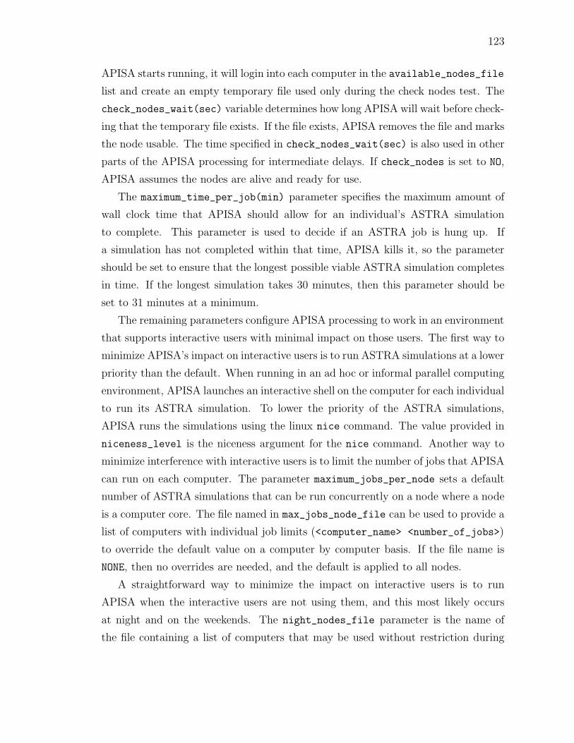
123

APISA starts running, it will login into each computer in the available_nodes_file

list and create an empty temporary file used only during the check nodes test. The

check_nodes_wait(sec) variable determines how long APISA will wait before check-

ing that the temporary file exists. If the file exists, APISA removes the file and marks

the node usable. The time specified in check_nodes_wait(sec) is also used in other

parts of the APISA processing for intermediate delays. If check_nodes is set to NO,

APISA assumes the nodes are alive and ready for use.

The maximum_time_per_job(min) parameter specifies the maximum amount of

wall clock time that APISA should allow for an individual’s ASTRA simulation

to complete. This parameter is used to decide if an ASTRA job is hung up. If

a simulation has not completed within that time, APISA kills it, so the parameter

should be set to ensure that the longest possible viable ASTRA simulation completes

in time. If the longest simulation takes 30 minutes, then this parameter should be

set to 31 minutes at a minimum.

The remaining parameters configure APISA processing to work in an environment

that supports interactive users with minimal impact on those users. The first way to

minimize APISA’s impact on interactive users is to run ASTRA simulations at a lower

priority than the default. When running in an ad hoc or informal parallel computing

environment, APISA launches an interactive shell on the computer for each individual

to run its ASTRA simulation. To lower the priority of the ASTRA simulations,

APISA runs the simulations using the linux nice command. The value provided in

niceness_level is the niceness argument for the nice command. Another way to

minimize interference with interactive users is to limit the number of jobs that APISA

can run on each computer. The parameter maximum_jobs_per_node sets a default

number of ASTRA simulations that can be run concurrently on a node where a node

is a computer core. The file named in max_jobs_node_file can be used to provide a

list of computers with individual job limits (<computer_name> <number_of_jobs>)

to override the default value on a computer by computer basis. If the file name is

NONE, then no overrides are needed, and the default is applied to all nodes.

A straightforward way to minimize the impact on interactive users is to run

APISA when the interactive users are not using them, and this most likely occurs

at night and on the weekends. The night_nodes_file parameter is the name of

the file containing a list of computers that may be used without restriction during

124

these times. The night_nodes_file list of computers must appear in the mas-

ter list of computers found in the available_nodes_file list. If the file name in

night_nodes_file is something other than NONE, APISA checks the current time

of day and day of the week for the after hours condition, and for computers in the

night nodes list, APISA will send jobs to those computers during off-hours but not

otherwise.

APISA can also be directed to monitor the usage of computers to see

if they can support running ASTRA simulations. The last four parameters,

use_unused_nodes_only, users_usage_threshold, system_usage_threshold,

and node_inactive_wait(min), work together to set up this mode of operation.

The first parameter is set to YES or NO. When set to NO, APISA may use comput-

ers listed in the available_nodes_file list without restrictions. When set to YES,

APISA uses the thresholds and time provided in the other three variables to deter-

mine if a computer is unused. If the user and system usage values as determined from

the linux command mpstat are below the thresholds and remain below the thresh-

olds for the specified amount of time, then APISA uses the computer until the user

and system usages increase above the threshold. If these increases happen during an

ASTRA simulation, the simulation process is killed.

C.4 DISTRIBUTION GENERATION IN APISA

As stated previously, it is possible to have APISA generate initial particle distri-

butions to use in its ASTRA runs [13]. ASTRA provides a tool to generate initial

particle distributions, but APISA does not use it. It can use ASTRA generated dis-

tributions as a fixed element of the optimization. If the user wants to vary the initial

particle distribution as part of the optimization, APISA generates its own subject to

parameters provided by the user as decision variables. The distributions that APISA

generates are radially symmetric (cylinders) and simulate particles emitted from a

photocathode. The settings for these distribution characteristics default to zero.

Some features of the particle distribution are not configurable. The angular dis-

tribution (θ) for the particle radial position is uniformly distributed over the range

0 to 2π. A particle’s transverse position is calculated in polar coordinates and then

converted to Cartesian coordinates. The longitudinal position (z) and momentum

(pz) are uniformly zero, corresponding to all particles being emitted from the cathode

surface located at z = 0.

125

The transverse momentum distributions (px, py) are determined by the Maxwell-

Boltzmann distribution to simulate thermal electrons. The general expression for

this distribution is

f (px, py, pz) =exp

(

−p2x+p2y+p2z2mkT

)

3√2πmkT

. (56)

The configuration parameter is the distribution thermal energy in meV (DIST_kT).

A so-called double-peak super-gaussian distribution is used to define the particle

distribution time and radial profiles. The time distribution corresponds to time emit-

ted from the photocathode. The parameters to define the distribution characteristics

are

DIST_XYtail

DIST_XYdip

DIST_XYellips

DIST_Ttail

DIST_Tdip

DIST_Tellips

DIST_Tslope

These control parameters can vary between 0 and 1. The tail variables, DIST_XYtail

for the transverse distribution and DIST_Ttail for the time distribution, describe the

size and shape of the distribution tails relative to its extent. Zero creates a distri-

bution with no tails, and one leads to Gaussian shaped tails. Figure 39(a) provides

illustrative examples. The dip variables, DIST_XYdip and DIST_Tdip, control the

overlap between the two peaks in the double peak distribution. Zero gives a flattop,

and the two peaks are merged to form one broad flattop profile. One means there are

two distinct peaks as shown in Figure 39(b). The ellipse parameters, DIST_XYellips

and DIST_Tellips, refer to the curvature of the flattop region. For zero, there is no

curvature (top hat), while one leads to an ellipse. This progression is clear in Figure

39(c).

The distribution in time has an additional control for slope, DIST_Tslope. This

parameter changes the relative heights of the peaks in the double peak distribution.

It skews the distribution relative to the first peak. If the slope is zero, the two peaks

are of equal height or as in Figure 39(d) where there is only one flattop peak, a flat

line. For a slope of one, the first peak is increased, and the second peak is greatly

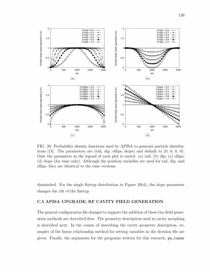
126

0

0.5

1

1.5

2

0 500 1000 1500 2000

Dou

ble-

peak

sup

er-g

auss

ian

p.d.

f.

bin

XYtail = 0.0XYtail = 0.2XYtail = 0.4XYtail = 0.6XYtail = 0.8XYtail = 1.0

(a)

0

0.5

1

1.5

2

0 500 1000 1500 2000

Dou

ble-

peak

sup

er-g

auss

ian

p.d.

f.

bin

XYdip = 0.0XYdip = 0.2XYdip = 0.4XYdip = 0.6XYdip = 0.8XYdip = 1.0

(b)

0

0.5

1

1.5

2

0 500 1000 1500 2000

Dou

ble-

peak

sup

er-g

auss

ian

p.d.

f.

bin

XYellips = 0.0XYellips = 0.2XYellips = 0.4XYellips = 0.6XYellips = 0.8XYellips = 1.0

(c)

0

0.5

1

1.5

2

0 500 1000 1500 2000

Dou

ble-

peak

sup

er-g

auss

ian

p.d.

f.

bin

Tslope = 0.0Tslope = 0.2Tslope = 0.4Tslope = 0.6Tslope = 0.8Tslope = 1.0

(d)

FIG. 39: Probability density functions used by APISA to generate particle distribu-tions [13]. The parameters are (tail, dip, ellips, slope) and default to (0, 0, 0, 0).Only the parameter in the legend of each plot is varied: (a) tail; (b) dip; (c) ellips;(d) slope (for time only). Although the position variables are used for tail, dip, andellips, they are identical to the time versions.

diminished. For the single flattop distribution in Figure 39(d), the slope parameter

changes the tilt of the flattop.

C.5 APISA UPGRADE: RF CAVITY FIELD GENERATION

The general configuration file changes to support the addition of these two field gener-

ation methods are described first. The geometry description used in cavity morphing

is described next. In the course of describing the cavity geometry description, ex-

amples of the linear relationship method for setting variables in the decision file are

given. Finally, the arguments for the programs written for this research, ps_tuner

127

and xvfb_manager, complete this appendix.

The communication, variator, and selector configuration files are unchanged

from the original APISA files. The diagnostic file, spea2_diag.log, additionally in-

cludes the values for the objectives and constraints evaluations for the non-dominated

individuals in the archive. The problem type in the variator parameter file remains

ASTRA since the field generation methods are optional.

The main changes are to the ASTRA set up file. There are eleven additions. An

example of the new ASTRA set up file is

astra_binary /full/path/to/ASTRA/executable/Astra

astra_input_file /full/path/to/ASTRA/input/file/gun.in

available_nodes_file /full/path/to/computer/list/nodes_list

remote_shell_mode ssh

night_nodes_file NONE

max_jobs_node_file NONE

check_nodes YES

check_nodes_wait(sec) 30

maximum_time_per_job(min) 6000

maximum_jobs_per_node 1

keep_in_purgatory(sec) 60

niceness_level 0

use_unused_nodes_only NO

users_usage_threshold 25.0

system_usage_threshold 25.0

node_inactive_wait(min) 15.0

generate_distributions NO

append_results_file /full/path/for/debug/data/RESULTS

distribution_directory /full/path/for/new/distributions/dist

number_particles 1000

particle_loss_output_names_file /full/path/for/loss/names

passive_particle_loss_ok NO

backward_traveling_particle_ok NO

particle_loss_before_zmin_ok YES

cathode_field_particle_loss_ok NO

aperture_particle_loss_ok YES

128

generate_efield_profile YES

efield_generation_method MORPH_EFIELD

efield_profile_directory /full/path/for/new/profiles/fields

efield_config_file /full/path/to/field/cfg/efld_config

astra_output_names_file /full/path/to/ASTRA/out/data/ast_name

decision_variables_file /full/path/to/decision/cfg/decisions

objectives_file /full/path/to/objective/cfg/objectives

constraints_file /full/path/to/constraint/cfg/constraints

Four additions, generate_efield_profile, efield_generation_method,

efield_profile_directory, and efield_config_file, relate to field generation.

The generate_efield_profile and efield_profile_directory parallel those for

the particle distribution option in the original APISA. The first parameter takes

a YES/NO value indicating whether or not APISA creates field profiles for each in-

dividual, and the second names where APISA writes the field profiles. The field

profiles generated are named the same way the ASTRA input and generated par-

ticle distribution files are named (e.g. gun.000000008.computer1.fld). If APISA

is creating field profiles, the efield_generation_method parameter tells APISA

which field creation method to use. The MORPH_EFIELD value directs APISA to

use field morphing, and the MORPH_GEOMETRY value directs APISA to use geometry

morphing. Another file is created for each individual that has a .info extension

(gun.000000008.computer1.fld.info), and the information written to the file de-

pends on the method chosen. The fourth parameter, efield_config_file, contains

configuration information relevant to the field creation method. The specifics of this

file and the contents of the .info file will be discussed later in C.5.1 and C.5.2.

There are five parameters in the ASTRA set up file to indicate which,

if any, particle loss mechanisms the optimization will allow. The pa-

rameters are passive_particle_loss_ok, backward_traveling_particle_ok,

particle_loss_before_zmin_ok, cathode_field_particle_loss_ok,

and aperture_particle_loss_ok. For each parameter that is set to YES, the

optimization uses ASTRA simulation results with the allowed loss mechanisms;

otherwise, the ASTRA simulation results are marked invalid. Similar to the

astra_output_names_file variable, the particle_loss_output_names_file pa-

rameter provides names for the particle loss variables, so they can be used in the

optimization. Here is a listing of the contents of an example file

129

passive_particle_losses

backward_traveling_particles

particles_lost_before_zmin

particles_lost_due_to_cathode_field

aperture_losses

These are included in the information written to the append_results_file file.

A minor addition is related to running interactive shells on linux computers.

There are two ways to login into a computer remotely: Remote Shell (rsh) and

Secure Shell (ssh). For computer security reasons, Secure Shell is preferred but is

not always supported. The remote_shell_mode parameter allows the user to choose

which shell tool to use when running APISA using interactive logins.

Next, the configuration and output related to each method is discussed after the

common parameters are described, followed by individual discussions of the field

creation specific parameters.

The common parameters are shown in Table 10. For either method, the file named

in efield_config_file must contain cavity_id and EFIELD_cav<cid>_npts

where <cid> is replaced with the setting in cavity_id. The field profiles are

on-axis profiles, Ez(r = 0, z) versus z in meters. The cavity_id parame-

ter must appear first in the file since its value is used to read all other field

variables in the file. The EFIELD_cav<cid>_npts is also required. However,

EFIELD_cav<cid>_update_ASTRA_freq is optional. If it is left unspecified, the fre-

quency in ASTRA input files is updated.

C.5.1 FIELD MORPHING

The input parameters for the field morphing method are based on the formula for the

morphing function, fmorphing (z), the number of cells, ncells, and the source frequency,

fsource. The equation for fmorphing (z) is repeated here for reference.

fmorphing (z) = 1 +

15∑

n=1

an cos

(

2πnz

Lcavity

)

+

15∑

n=1

bn sin

(

2πnz

Lcavity

)

The input parameters for the field morphing method are listed in Table 11. It is

assumed that gun cells are constructed of full cells and optionally preceded by a

fractional cell. For example, if EFIELD_cav<cid>_ncells has the value 1.5, then

Eπapprox(z) is a partial sine wave that extends from 45◦ to 180◦. The parameters in

130

TABLE 10: Common field generation input parameters

Parameter Purpose Value

cavity_id Cavity identificationnumber. It is thesame as the indexused in the CAVITYsection of the ASTRAinput file. The valueof this parameter isused in the name ofsubsequentparameters.

positiveinteger

EFIELD_cav<cid>_npts The number of pointsto produce for thefield profile for cavity<cid>.

positiveinteger

EFIELD_cav<cid>_update_ASTRA_freq Indicates whether ornot for cavity <cid>,APISA should updatethe ASTRA input fileto use the calculatedfrequency (YES) or letit be fixed (NO)

YES

(default)or NO

131

TABLE 11: Field morphing input parameters

Parameter EquationComponent

Value

EFIELD_MORPH_cav<cid>_A<1-15> an real number

EFIELD_MORPH_cav<cid>_B<1-15> bn real number

EFIELD_cav<cid>_ncells ncells positive realnumber

EFIELD_MORPH_cav<cid>_source_freq fsource inHertz

positive realnumber

Tables 10 and 11 may appear in the file named in efield_config_file or a decision

variable file (but not both). An example field configuration file is

cavity_id 1

EFIELD_cav1_ncells 1.5

EFIELD_MORPH_cav1_source_freq 1300e6

EFIELD_cav1_npts 1000

EFIELD_MORPH_cav1_A1 0.5

EFIELD_MORPH_cav1_B2 0.35

In this example, APISA creates 1000 point field profiles for ASTRA cavity number

one. The field profile approximates the π mode of a one and a half cell structure

using fsource equal to 1300 MHz. The two coefficients, a1 and b2, of fmorphing (z) are

fixed at 0.5 and 0.35, respectively. A sample decision variable file using parameters

from the table is

EFIELD_MORPH_cav1_A2 VARY 0 0.25

EFIELD_MORPH_cav1_A3 VARY 0 0.75

EFIELD_MORPH_cav1_B3 VARY 0 0.50

EFIELD_MORPH_cav1_B4 VARY 0 0.30

Used in conjunction with the field configuration file, the Fourier coefficients listed as

decision variables, a2, a3, b3, and b4, are varied in the optimization as specified while

a1 and b2 are fixed to the values listed in the field configuration file. The rest of the

coefficients, a4 through a15, b1, and b5 through b15, are set to zero.

132

TABLE 12: All field profile characteristics provided by the field morphing method

Parameter name

(prefix EFIELD_MORPH_cav<cid>_) Method of Calculation

AN_SUM15∑

n=1

an

ANFN_MAX max

[

15∑

n=1

an cos(

2πn zLcavity

)

]

ANFN_MIN min

[

15∑

n=1

an cos(

2πn zLcavity

)

]

BN_SUM15∑

n=1

bn

BNFN_MAX max

[

15∑

n=1

bn sin(

2πn zLcavity

)

]

BNFN_MIN min

[

15∑

n=1

bn sin(

2πn zLcavity

)

]

EFIELD_MAX max [Ez (z)]

EFIELD_MIN min [Ez (z)]

EFIELD_FREQ_GHZ Frequency of Ez (z)determined via Fast FourierTransform

F_COEFF_SUM15∑

n=1

an +15∑

n=1

bn

MORPHINGFN_MAX max [fmorphing (z)]

MORPHINGFN_MIN min [fmorphing (z)]

Characteristics of the resulting Fourier series function and the field profile gen-

erated are provided to the optimization and can be used in constraints or objec-

tives files. These are written to the .info file and included in the output to the

append_results_file file. Table 12 lists the available parameters. A constraint to

ensure that the morphing function is above the z = 0 axis as mentioned in 3.3.1 for

cavity 1 is

EFIELD_MORPH_cav1_MORPHINGFN_MIN GREATER_THAN 0.0

In addition to the .info file, a diagnostic gnuplot [93] command file is created

for each individual with the .gpl extension. The Fourier coefficients used to create

the field profile are included in the comments of the command file for reference.

133

The file also contains the data and gnuplot commands to plot Eπapprox(z), Ez (z),

the an dependent term in fmorphing (z), the bn dependent term in fmorphing (z), and

fmorphing (z). Unless a version of the variator executable is run that does not remove

intermediate files, these diagnostic gnuplot files are not available after APISA finishes

processing.

C.5.2 GEOMETRY MORPHING

The cavity geometry morphing field configuration file contains more administrative

information like the ASTRA set up file than the field morphing version. This is

because cavity morphing follows the ASTRA processing model. It modifies a cavity

geometry file and then passes it to a program to produce the field profile. In field

morphing, each field profile is computed on the fly directly by APISA before launching

the ASTRA simulation. Rather than list the parameters in a table, they are discussed

individually. An example file is

cavity_id 1

EFIELD_cav1_npts 1000

EFIELD_GEOMETRY_cav1_description /path/to/cav_desc.txt

EFIELD_GEOMETRY_field_variables_list /path/to/PS/outvars.txt

EFIELD_GEOMETRY_helper_program_directory /path/to/PS/programs

EFIELD_cav1_update_ASTRA_freq YES

EFIELD_GEOMETRY_cav1_history_file /path/to/GeomHistory

EFIELD_GEOMETRY_cav1_rescale_MaxE YES

EFIELD_GEOMETRY_cav1_rescale_peak_number 1

The generalized cavity description that APISA is to use as a template is named

in EFIELD_GEOMETRY_cav1_description. The name of the file containing the ex-

pected list of output variables from the Poisson Superfish processing is given in

EFIELD_GEOMETRY_field_variables_list. A sample subset listing contains

FIELDFLATNESS

FREQ

PiMode

SIGNED_FIELDFLATNESS

These are described in the ps_tuner discussion below and appear in the

append_results_file output. APISA needs to know where ps_tuner, the program

134

to run Poisson Superfish, and xvfb_manager are located. The directory location

for these programs is provided in EFIELD_GEOMETRY_helper_program_directory.

The EFIELD_GEOMETRY_cav1_history_file parameter gives the filename where

APISA records the geometry descriptions that lead to π modes. If it is set to

NONE, the geometries are not recorded. EFIELD_GEOMETRY_cav1_rescale_MaxE

and EFIELD_GEOMETRY_cav1_rescale_peak_number are related. The first indicates

whether or not the MaxE(1) parameter in the ASTRA input file should be rescaled

to guarantee that a particular peak in the generated field profile has the intended

value of MaxE(1). If it is set to NO, then MaxE(1) is not rescaled. If it is set

to YES, MaxE(1) is rescaled so that the peak number (counting from 1) noted in

EFIELD_GEOMETRY_cav1_rescale_peak_number is scaled to the value of MaxE(1) in

the ASTRA input file. This value of MaxE(1) may be fixed or a newly generated

value if MaxE(1) is a decision variable.

Generalized geometry description

The geometry description file is discussed next. The geometry description breaks

a cavity into a series of beam tubes and cells. These building blocks and their

components are shown in Figure 40. There are additional elements for the search

frequency and drive point location. Each building block is described with examples.

A list of permissible and default units follows. Finally, naming for cavity components

in decision variables is discussed including example uses of the linear relationship

method for setting variables.

The cell element name is pillbox_cell. Each cell section starts with a

pillbox_cell keyword and ends with pillbox_cell end. Between these are the

components and their settings. An example pillbox cell with an exit iris is shown in

Table 13. This creates a pillbox cavity with a 9 cm radius that can be used as a gun

cell. The cell is 5.5 cm in length from entrance to exit. The entrance wall extends

to the symmetry axis. The exit wall stops 2.5 cm above the symmetry axis creating

the exit iris for the cell. The pillbox cavity can be changed to a re-entrant cell with

entrance and exit tubes. This is shown in Table 14. Adding the entrance iris offset

causes an entrance beam tube to be added. Nonzero wall angles tilt the walls, in this

case, toward each other. Making the neck width smaller than the main cell width

makes the opening to the beam tube smaller than the main cell width. The neck

and cell offsets move the base of the main cell away from the symmetry axis. All of

135

Radius

Length

(a)

Cell radius

Neck width

Cell base width

Cell offsets

Radii of irises

Neck offsets

Entrance wall Exit wall

Cell wall angles -90o < θ < 90o

(b)

FIG. 40: Cavity and beam tube layout for geometry description [12]: (a) beamtube or iris; (b) cell (Figure 9 reproduced for convenience). The beam enters eachelement from the left. The axis across the bottom is the axis of rotation and typicallycorresponds to the beam axis. The components of the cell on the left side are calledentrance quantities. The exit quantities are on the right.

the changes here are mirror symmetric, but they do not have to be. The entrance

values do not have to match the exit values (or only differ by a sign). They can be

set independently.

There is a separate beam tube element called the tube_iris. Its block is struc-

tured the same way, but it only has two components. An example file for a one cell

pillbox cavity with a downstream beam tube is in Table 15.

The elements have units associated with them. The accepted units for length and

their abbreviations are inches (in), millimeters (mm), centimeters (cm). If a length unit

is omitted, the default, centimeters, is assumed. For frequency, the permissible units

are hertz (Hz), kilohertz (kHz), megahertz (MHz), and gigahertz (GHz). The default

is megahertz. For angles, degrees and radians are accepted, and the default is

degrees. All units are converted to the default units, and the Poisson Superfish file

generated uses the default units. Here is the example in Table 15 expanded to use

the frequency and optional drive point location elements

frequency 1300 MHz

major_element_for_drive_point 2

pillbox_cell

cell_radius 9 cm

136

TABLE 13: Pillbox geometry examplepillbox_cell

cell_radius 9 cm

iris_entrance_wall_radius 0 cm

iris_exit_wall_radius 2.5 cm

cell_base_width 5.5 cm

cell_base_entrance_wall_angle 0 degrees

cell_base_entrance_wall_offset 0 cm

cell_base_exit_wall_angle 0 degrees

cell_base_exit_wall_offset 0 cm

neck_width 5.5 cm

neck_entrance_wall_offset 0 cm

neck_exit_wall_offset 0 cm

pillbox_cell end

TABLE 14: Re-entrant cavity geometry example based on pillbox examplepillbox_cell

cell_radius 9 cm

iris_entrance_wall_radius 2.5 cm

iris_exit_wall_radius 2.5 cm

cell_base_width 5.5 cm

cell_base_entrance_wall_angle 10 degrees

cell_base_entrance_wall_offset 1 cm

cell_base_exit_wall_angle -10 degrees

cell_base_exit_wall_offset 1 cm

neck_width 3.5 cm

neck_entrance_wall_offset 0.5 cm

neck_exit_wall_offset 0.5 cm

pillbox_cell end

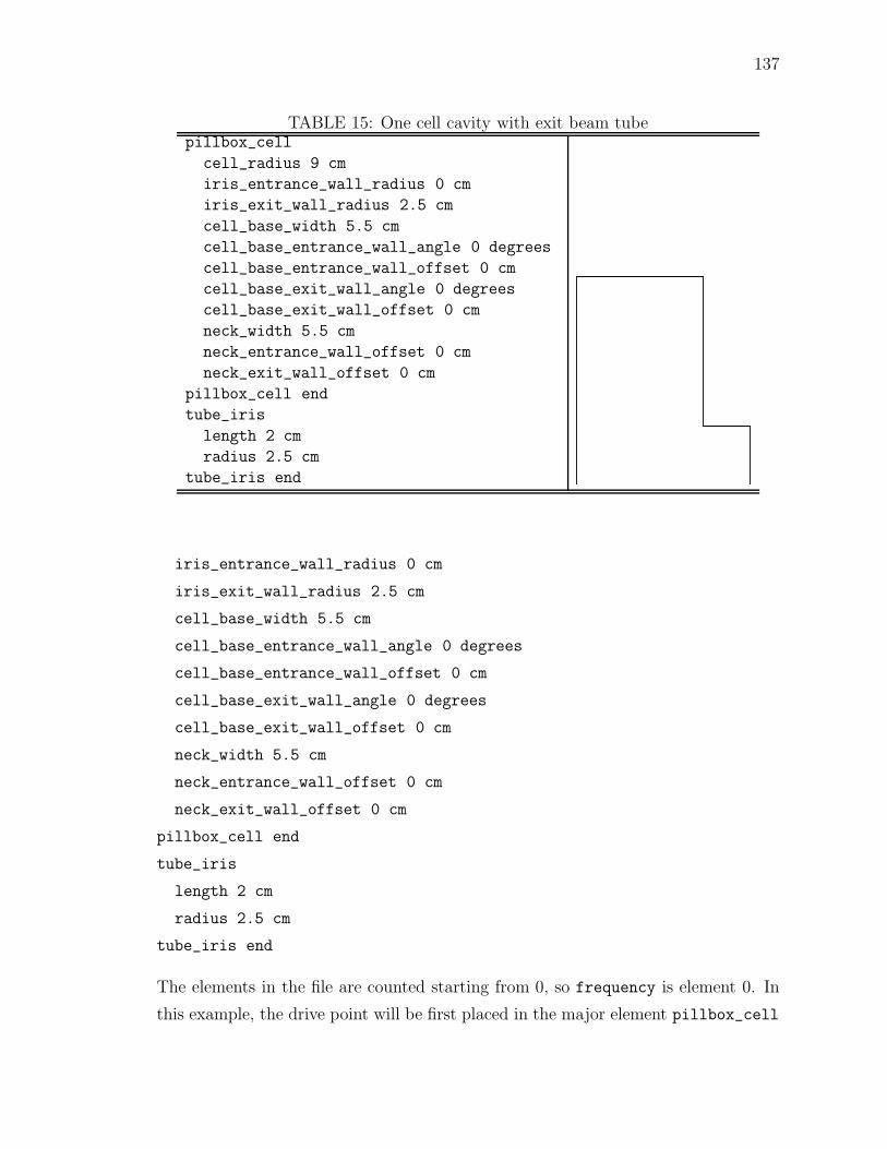
137

TABLE 15: One cell cavity with exit beam tubepillbox_cell

cell_radius 9 cm

iris_entrance_wall_radius 0 cm

iris_exit_wall_radius 2.5 cm

cell_base_width 5.5 cm

cell_base_entrance_wall_angle 0 degrees

cell_base_entrance_wall_offset 0 cm

cell_base_exit_wall_angle 0 degrees

cell_base_exit_wall_offset 0 cm

neck_width 5.5 cm

neck_entrance_wall_offset 0 cm

neck_exit_wall_offset 0 cm

pillbox_cell end

tube_iris

length 2 cm

radius 2.5 cm

tube_iris end

iris_entrance_wall_radius 0 cm

iris_exit_wall_radius 2.5 cm

cell_base_width 5.5 cm

cell_base_entrance_wall_angle 0 degrees

cell_base_entrance_wall_offset 0 cm

cell_base_exit_wall_angle 0 degrees

cell_base_exit_wall_offset 0 cm

neck_width 5.5 cm

neck_entrance_wall_offset 0 cm

neck_exit_wall_offset 0 cm

pillbox_cell end

tube_iris

length 2 cm

radius 2.5 cm

tube_iris end

The elements in the file are counted starting from 0, so frequency is element 0. In

this example, the drive point will be first placed in the major element pillbox_cell

138

during the π mode search, and that is element number 2 in the file. A major element

is a pillbox_cell or a tube_iris.

Some name mangling is needed to use a parameter in the cavity geometry file as

a decision variable in the optimization. To uniquely identify which parameter in the

cavity geometry file is to be changed, the decision variable name includes the cavity

identification number, the cavity element location, and the dimension. An example

decision file based on the example in Table 15 is

cav1-tube_iris1-radius VARY 1.5 5

cav1-pillbox_cell1-iris_exit_wall_radius LINEAR

cav1-tube_iris1-radius SLOPE 1 OFFSET 0

The first variable name points to the radius feature in the first tube_iris element in

the cavity description file for cavity one. Further it directs APISA to vary this dimen-

sion between 1.5 and 5 cm. The second line points to the iris_exit_wall_radius

feature of the first pillbox_cell element in the cavity one description file. Note

that the line break in the second entry is not permitted in decision, constraint, and

objective files. This example shows how a variable can be made linearly related to

another one and how the optimizer can set neighboring elements as described in 3.3.2.

To create a symmetric re-entrant cell as mentioned in 3.3.3, if the opti-

mization is varying the cell_base_entrance_wall_angle in Table 14, then the

cell_base_exit_wall_angle can be made to track the first using

cav1-pillbox_cell1-cell_base_entrance_wall_angle VARY 10 -10

cav1-pillbox_cell1-cell_base_exit_wall_angle

LINEAR cav1-pillbox_cell1-cell_base_entrance_wall_angle

SLOPE -1 OFFSET 0

The entrance wall angle is varied between −10◦ and 10◦, and the exit angle is set

to track it but with the opposite sign. If the entrance wall tilts outward (negative

angle), so will the exit wall with the corresponding positive angle.

The linear relationship can use used to implement the APISA example in C.3

where one MaxB is made equal to another. Using the linear relationship, it can be

written as

MaxB(1) VARY -0.179 -0.168

MaxB(2) VARY |-> MaxB(1) 0.5 1.0

MaxB(3) LINEAR MaxB(1) SLOPE 0 OFFSET 0

139

Here, the decision variable count is two instead of three.

ps tuner program

For cavity field generation, APISA calls the ps_tuner program. It handles all Poisson

Superfish related processing from producing Poisson Superfish geometry files for the

building block geometry description to running the Poisson Superfish programs to

find the π mode field profile. It uses one input file from the user and if running under

Wine another from the xvfb_manager program. ps_tuner produces four output files.

The arguments for the program are described after the output files, and the input

files are described last.

Each output file is named according to the geometry file that ps_tuner is con-

verting. Filename suffixes are used to differentiate the files. The first output file

is the field profile for the π mode ps_tuner finds or a zero profile if no π mode is

found. The second file is the .info file. It contains information extracted or derived

from the Poisson Superfish output files. A representative subset of this information

is in Table 16. The third file is the .peaks file. This provides the normalized peak

amplitudes in the field profile. MaxE rescaling uses this information. The last file

is _new.cfg and is a record of the building block description that produced the π

mode. The main differences between the new config file and the original description

are the units of the elements, the search frequency, and the drive point location.

The ps_tuner program works with the default units named previously, and the new

configuration file reflects that.

The ps_tuner program has several arguments shown in Table 17. A typical

calling sequence is

ps_tuner -a -p 45 -c cav_desc.txt

This directs ps_tuner to run Poisson Superfish under Wine and to use the Xvfb

process associated with process identification 45. It takes the geometry descrip-

tion cav_desc.txt and produces output files cav_desc.fld for the field profile,

cav_desc.fld.info for the associated field characteristics, cav_desc.fld.peaks

for the normalized peak amplitudes for field profile, and cav_desc_new.cfg for the

final geometry description.

140

TABLE 16: Sample ps tuner provided information

Output name Description

FIELDFLATNESS Using ncells determined from thegeometry description,un-normalized peak informationfor the field profile for |Epeak|max,|Epeak|min, and |Epeak|i,field flatness =

100|Epeak|

max−|Epeak|

min

1ncells

(ncells∑

i=1|Epeak|

i

)

FREQ Resonance frequency for thegeometry calculated by thePoisson Superfish program fish

PiMode Indicates if ps_tuner found a πmode (1) or not (0).

SIGNED_FIELDFLATNESS Same as FIELDFLATNESSexcept the sign is derived fromthe relative position of theminimum and maximum peaks.If the maximum is to the left ofthe minimum, the sign isnegative; otherwise, it is positive.

141

TABLE 17: ps tuner arguments and descriptions

Argument Name Description

-a add Add the .fld extension to the fieldprofile, info, and peaks file names

-c filename configuration Name of the general cavity description.The path name may be included. If it isnot, the program looks for the file in thepresent working directory. It is assumedthat the filename has an extension suchas .txt or .cfg. The base name of thefile (name minus any extension) is usedas the base name for the output files.

-d path directory The full directory path to the locationwhere ps_tuner should run and putresults. If it is omitted, the programwrites the output files to the presentworking directory.

-e cygwin|wine environment The program runs under Wine on linuxand Cygwin [94] in Windows. Thedefault environment Wine is assumed.Running under Wine requires the -p flag.

-i cid identification The names of the output parameterswritten to the info file are prependedwith EFIELD_GEOMETRY_cav<cid>_.Using this option allows the info filevalues to be used in objectives andconstraints.

-k clean Do not clean up intermediate files anddirectories the program creates. This isoverridden by APISA.

-p pid pid The process identification (pid) of theprogram that calls ps_tuner. This isonly needed for running under Wine. Itidentifies which xvfb_manager

information file should be checked forXvfb display information.

-t table_size table The number of (z, Ez (r = 0, z)) pairs towrite out for the field profile.

-v verbose Print debug information

142

TABLE 18: xvfb manager arguments and descriptions

Argument Name Description

-k kill Kill the Xvfb process associated with theprocess identification named in the pidargument. This cannot be used with the-l option.

-l launch Launch an Xvfb process for the processidentification named in the pid argumentas necessary. This cannot be used withthe -k option.

-p pid pid The process identification number withwhich to associate the Xvfb process.This is required.

xvfb manager program

APISA uses the xvfb_manager program to manage the Xvfb processes that instances

of ps_tuner need in order to run Poisson Superfish under Wine. Its purpose is to

launch and kill Xvfb processes. It has no user provided input files and produces

two specially named output files, a lock file and a data file. The arguments for

the program are listed in Table 18. The xvfb_manager processing is discussed next

followed by a description of the input files.

When the xvfb_manager program is directed to launch an Xvfb process, it first

checks to see if the data file for the provided process identification exists in the

current working directory. If the file exists, the program reads the display number

from it. The program checks to see if there is a matching Xvfb process running for

the user calling the program. If the correct Xvfb process is running, the program

does nothing, but if the Xvfb process is not running, it starts it. In this mode,

xvfb_manager acts as a restart mechanism. When there is no data file, the program

cycles through display numbers searching for one that is available for the user calling

the program. Once it finds an unused display number, it writes the number to the

data file and launches the appropriate Xvfb process.

Processing for killing an Xvfb process is much simpler. The xvfb_manager pro-

gram reads the data file to determine which Xvfb process to kill in the event that

several Xvfb processes are running for a particular user. It kills the Xvfb process

143

with the designated display owned by the user calling the program. It then removes

the data file and exits.

The output files are named xvfb_manager_<pid>_<computer name>.info for

the data file and xvfb_manager_<pid>_<computer name>.lck for the lock file. The

process identification, <pid>, is provided as an argument to xvfb_manager. The

computer name is the name of the computer where xvfb_manager is running and

is determined from the operating system. These files also serve as input files to

the xvfb_manager program. The lock file exists only while xvfb_manager is run-

ning. Each instance of xvfb_manager checks if a lock file with the provided process

identification exists in the current working directory before processing. If it does,

the program does nothing and exits under the assumption that another instance of

xvfb_manager is manipulating the Xvfb processing. If it does not find the file, it

creates one, performs the required Xvfb processing, removes the lock file, and then

exits. The data file contains the X Windows display number for the Xvfb process

launched by an xvfb_manager program for the provided process identification.

Here are two examples of running the xvfb_manager program. They both refer

to pid 45. The first example launches an Xvfb process

xvfb_manager -p 45 -l

The second one kills an Xvfb process

xvfb_manager -p 45 -k

144

VITA

Alicia S. Hofler

Department of Electrical and Computer Engineering

Old Dominion University

Norfolk, VA 23529

ACADEMIC PREPARATION

• Ph.D., Electrical and Computer Engineering Department, Old Dominion Uni-

versity, Norfolk, Virginia, May, 2012

• M.E., Electrical and Computer Engineering Department, Old Dominion Uni-

versity, Norfolk, Virginia, August, 2001

• B.A., Physics Department, Randolph-Macon Woman’s College, Lynchburg,

Virginia, May, 1987

PROFESSIONAL EXPERIENCE

• Jefferson Lab, Staff Computer Scientist, May 1992 - present. Currently re-

sponsible for improving injector performance of the Continuous Electron Beam

Accelerator with model development and multi-objective optimization.

RECENT PUBLICATIONS

1. M. Kramer, et. al., in Physical Review Special Topics - Accelerator and Beams,

in preparation

2. S. Ahmed, et. al., in Physical Review Special Topics - Accelerator and Beams,

vol. 15, no. 3, 022001, 2012

3. A. Hofler and P. Evtushenko, in Proceedings of PAC11, New York City, New

York, March 2011

4. A. S. Hofler, P. Evtushenko, and F. Marhauser, in Proceedings of ICAP09, San

Francisco, California, August 2009

5. A. Hofler, P. Evtushenko, and M. Krasilnikov, in Proceedings of PAC07, Albu-

querque, New Mexico, August 2007

Typeset using LATEX.