Open Archive TOULOUSE Archive Ouverte (OATAO) OATAO is an open access repository that collects the work of Toulouse researchers and makes it freely available over the web where possible.

This is an author-deposited version published in : http://oatao.univ-toulouse.fr/ Eprints ID : 15676

To link to this article : DOI:10.1016/j.combustflame.2016.01.004 URL : http://dx.doi.org/10.1016/j.combustflame.2016.01.004

To cite this version : Mari, Raphaël and Cuenot, Bénédicte and Rocchi, Jean-Philippe and Selle, Laurent and Duchaine, Florent Effect of pressure on Hydrogen/Oxygen coupled flame-wall interaction. (2016) Combustion and Flame, vol. 168. pp. 409-419. ISSN 0010-2180

Any correspondence concerning this service should be sent to the repository

administrator: staff-oatao@listes-diff.inp-toulouse.fr

Effect of pressure on hydrogen/oxygen coupled flame–wall interaction

Raphael Mari a , ∗, Benedicte Cuenot a , Jean-Philippe Rocchi a , Laurent Selle b , Florent Duchaine a

a CERFACS, 42 av G. Coriolis, 31057 Toulouse, France b CNRS, IMFT, F-31400 Toulouse, France

Keywords:

Real-gas thermodynamics

Flame–wall interaction

Conjugate heat transfer

a b s t r a c t

The design and optimization of liquid-fuel rocket engines is a major scientific and technological chal-

lenge. One particularly critical issue is the heating of solid parts that are subjected to extremely high

heat fluxes when exposed to the flame. This in turn changes the injector lip temperature, leading to

possibly different flame behaviors and a fully coupled system. As the chamber pressure is usually much

larger than the critical pressure of the mixture, supercritical flow behaviors add even more complexity

to the thermal problem. When simulating such phenomena, these thermodynamic conditions raise both

modeling and numerical specific issues. In this paper, both subcritical and supercritical hydrogen/oxygen

one-dimensional, laminar flames interacting with solid walls are studied by use of conjugate heat transfer

simulations, allowing to evaluate the wall heat flux and temperature, their impact on the flame as well

as their sensitivity to high pressure and real gas thermodynamics up to 100 bar where real gas effects

are important. At low pressure, results are found in good agreement with previous studies in terms of

wall heat flux and quenching distance, and the wall stays close to isothermal. On the contrary, due to

important changes of the fluid transport properties and the flame characteristics, the wall experiences

significant heating at high pressure condition and the flame behavior is modified.

1. Introduction

Most of high performance propulsion devices such as turbines,

rocket engines or scramjets operate in wall-bounded flows. The

interaction between flame and walls has a direct and strong im-

pact on combustion, pollutant emissions and combustion cham-

ber lifetime. Understanding the mechanisms at play in flame–wall

interaction (FWI) is therefore necessary to further gain in per-

formance, safety, fuel consumption and unburnt gas emission. As

shown in [1,2] , local FWI may be described in simple laminar

flows where generic flame configurations may be introduced. Dur-

ing the flame–wall interaction process, the flame speed and thick-

ness decrease, before full quenching at a few microns away from

the wall. When the flame approaches the wall, the temperature

decreases from burnt gases (approximately 30 0 0 K for hydrogen

( H 2 )/oxygen( O 2 ) flames at 1 bar) to wall levels that are maintained

in the 30 0–80 0 K range to avoid damaging. This high tempera-

ture variation occurs in a very thin layer, less than 1 mm , leading

to very strong temperature gradients and making experimental ob-

servation of FWI quite difficult.

∗ Corresponding author.

E-mail address: raphael.mari.cerfacs@gmail.com (R. Mari).

Ezekoye et al. [3] experimentally studied the impact of wall

temperature and the equivalence ratio on the wall heat flux for

propane and methane flames. It was shown that the maximum

wall heat flux decreases when the wall temperature increases. Lu

et al. [4] investigated FWI in the side wall quenching configura-

tion where the flame propagates along the wall and found that

the ratio of the wall heat flux to the heat release in the flame is

roughly constant and equal to 0.3–0.4. Based on experimental cor-

relations, Boust et al. [5] proposed a theoretical relation between

the normalized wall heat flux and the quenching Peclet number,

defined as the flame position normalized by the flame thickness,

for methane-air flames where they observe that the wall heat flux

is inversely proportional to the flame quenching distance.

Many numerical studies have been conducted on laminar

flame–wall interactions [6–10] . It has been shown by Popp

et al. [9] that in the low wall temperature regime (300 K <

T w < 400 K) the wall can be assumed chemically inert. Kim

et al. [11] experimentally confirmed this result using several sur-

face materials and wall temperatures. Dabireau et al. [7] , Gruber

et al. [12] and Owston et al. [10] , demonstrated a strongly differ-

ent behavior for hydrogen flames compared to hydrocarbon flames.

Hydrogen flame quenching occurs much closer to the wall rela-

tively to the flame thickness. Normalized wall heat flux is also

largely different from hydrocarbon flames and equal to ∼0.12.

http://dx.doi.org/10.1016/j.combustflame.2016.01.004

Nomenclature

Symbol Units Description

C p J K −1 kg −1

Heat capacity

D th m 2 s −1 Thermal diffusivity

e J m −2 K −1 s −1 / 2 Effusivity

P c Pa Critical pressure

Pe – Peclet number based on heat release rate

Pe F – Peclet number based on fuel consumption rate

Q W m −3 Heat release rate

Q ∗ – Heat release rate non-dimensionalized with Q 0 l /δ

Q 0 l W m −2 Laminar flame power

S 0 l m s −1 Flame speed

Sc – Schmidt number

T c K Critical temperature

T S K Solid temperature

T w K Fluid-solid interface temperature

Z – Compressiblity factor

Greek symbols

δl m Thermal flame thickness

δ m Diffusive flame thickness

1H J kg −1

Heat per kg of fuel

κ – Ratio of wall and fluid effusivities

λ W m −1 K −1 Thermal conductivity

8w W m −2 Heat flux

8∗w – Heat flux non-dimensionalized with Q 0

l τ s Flame characteristic time

Superscripts IFF Infinitely Fast Flame C Coupled U Uncoupled b burnt u unburnt

Subscripts

Q quenching

w wall

In all these studies, results have been provided for wall bound-

ary conditions either adiabatic or isothermal. However in reality

heat transfer occurring between the solid wall and the fluid results

in a possible increase of wall temperature and a non-zero heat flux,

i.e. neither isothermal nor adiabatic wall behavior. In addition, the

wall temperature is usually unknown and introduces a significant

uncertainty on the predicted heat flux. Finally, FWI being a tran-

sient phenomenon, eventually leading to flame quenching, the so-

lution cannot be searched for as a steady state solution and sim-

ulations describing the unsteady coupling of heat conduction in

the wall with fluid dynamics and heat transfer are required [13] .

Such approach avoids to impose the wall temperature at an arbi-

trary value, and allows it to adapt to the varying fluid temperature,

consequently significantly modifying the wall heat flux.

To address this issue, the present study considers the unsteady

behavior of a stoichiometric laminar one-dimensional premixed

hydrogen–oxygen flame impinging on a cold wall including conju-

gate heat transfer. The context is liquid-fuel rocket engines (LREs),

which operate at very low temperature and high pressure where

the thermodynamic properties depart from ideal gas laws. Indeed,

beyond the critical point , defined by ( P c , T c ) values specific to each

species, surface tension disappears and the distinction between

gaseous and liquid phases vanishes. This state of matter is called

supercritical, where phase change is replaced by a steep but con-

tinuous variation of the density and thermodynamic properties.

Therefore the objective of the study is twofold: first, the role of

conjugate heat transfer in FWI is studied; second, the impact on

FWI of high pressure, up to supercritical conditions, is evaluated.

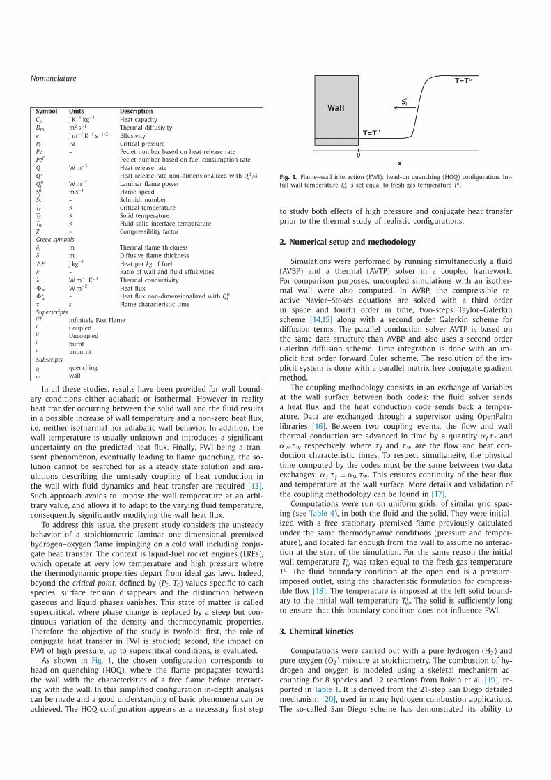
As shown in Fig. 1 , the chosen configuration corresponds to

head-on quenching (HOQ), where the flame propagates towards

the wall with the characteristics of a free flame before interact-

ing with the wall. In this simplified configuration in-depth analysis

can be made and a good understanding of basic phenomena can be

achieved. The HOQ configuration appears as a necessary first step

Fig. 1. Flame–wall interaction (FWI): head-on quenching (HOQ) configuration. Ini-

tial wall temperature T i w is set equal to fresh gas temperature T u .

to study both effects of high pressure and conjugate heat transfer

prior to the thermal study of realistic configurations.

2. Numerical setup and methodology

Simulations were performed by running simultaneously a fluid

(AVBP) and a thermal (AVTP) solver in a coupled framework.

For comparison purposes, uncoupled simulations with an isother-

mal wall were also computed. In AVBP, the compressible re-

active Navier–Stokes equations are solved with a third order

in space and fourth order in time, two-steps Taylor–Galerkin

scheme [14,15] along with a second order Galerkin scheme for

diffusion terms. The parallel conduction solver AVTP is based on

the same data structure than AVBP and also uses a second order

Galerkin diffusion scheme. Time integration is done with an im-

plicit first order forward Euler scheme. The resolution of the im-

plicit system is done with a parallel matrix free conjugate gradient

method.

The coupling methodology consists in an exchange of variables

at the wall surface between both codes: the fluid solver sends

a heat flux and the heat conduction code sends back a temper-

ature. Data are exchanged through a supervisor using OpenPalm

libraries [16] . Between two coupling events, the flow and wall

thermal conduction are advanced in time by a quantity αf τ f and

αw τw respectively, where τ f and τw are the flow and heat con-

duction characteristic times. To respect simultaneity, the physical

time computed by the codes must be the same between two data

exchanges: α f τ f = αw τw . This ensures continuity of the heat flux and temperature at the wall surface. More details and validation of

the coupling methodology can be found in [17] .

Computations were run on uniform grids, of similar grid spac-

ing (see Table 4 ), in both the fluid and the solid. They were initial-

ized with a free stationary premixed flame previously calculated

under the same thermodynamic conditions (pressure and temper-

ature), and located far enough from the wall to assume no interac-

tion at the start of the simulation. For the same reason the initial

wall temperature T i w was taken equal to the fresh gas temperature

T u . The fluid boundary condition at the open end is a pressure-

imposed outlet, using the characteristic formulation for compress-

ible flow [18] . The temperature is imposed at the left solid bound-

ary to the initial wall temperature T i w . The solid is sufficiently long

to ensure that this boundary condition does not influence FWI.

3. Chemical kinetics

Computations were carried out with a pure hydrogen ( H 2 ) and

pure oxygen ( O 2 ) mixture at stoichiometry. The combustion of hy-

drogen and oxygen is modeled using a skeletal mechanism ac-

counting for 8 species and 12 reactions from Boivin et al. [19] , re-

ported in Table 1 . It is derived from the 21-step San Diego detailed

mechanism [20] , used in many hydrogen combustion applications.

The so-called San Diego scheme has demonstrated its ability to

Fig. 2. 1D flame profiles of (a) temperature T , (b) heat release rate Q , (c) HO 2 and (d) H mass fractions for (–) San Diego [20] and (- -) Boivin [19] mechanisms. Case 2a:

pressure is 1 bar and fresh gas temperature 300 K.

Table 1

Rate coefficients in Arrhenius form k = AT n exp (−E/R 0 T ) as in [19] .

Reaction A a n E a

R1 H + O 2 ⇌ OH + O k f 3.52 10 16 −0 .7 71 .42

k b 7.04 10 13 −0 .26 0 .60

R2 H 2 + O ⇌ OH + H k f 5.06 10 4 2 .67 26 .32

k b 3.03 10 4 2 .63 20 .23

R3 H 2 + OH ⇌ H 2 O + H k f 1.17 10 9 1 .3 15 .21

k b 1.28 10 10 1 .19 78 .25

R4 H + O 2 + M → HO 2 + M b k 0 5.75 10 19 −1 .4 0 .0

k ∞ 4.65 10 12 0 .44 0 .0

R5 HO 2 + H → 2 OH 7.08 10 13 0 .0 1 .23

R6 HO 2 + OH ⇌ H 2 + O 2 k f 1.66 10 13 0 .0 3 .44

k b 2.69 10 12 0 .36 231 .86

R7 HO 2 + OH → H 2 O + O 2 2.89 10 13 0 .0 −2 .08 R8 H + OH + M ⇌ H 2 O + M c k f 4.00 10 22 −2 .0 0 .0

k b 1.03 10 23 −1 .75 496 .14

R9 2 H + M ⇌ H 2 + M c k f 1.30 10 18 −1 .0 0 .0

k b 3.04 10 17 −0 .65 433 .09

R10 2 HO 2 → H 2 O 2 + O 2 3.02 10 12 0 .0 5 .8

R11 HO 2 + H 2 → H 2 O 2 + H 1.62 10 11 0 .61 100 .14

R12 H 2 O 2 + M → 2 OH + M d k 0 8.15 10 23 −1 .9 207 .62

k ∞ 2.62 10 19 −1 .39 214 .74

a Units are mol, s, cm 3 , kJ and K. b Chaperon efficiencies H 2 : 2.5, H 2 O: 16.0, 1.0 for all other species. Troe falloff

with F c = 0 . 5 . c Chaperon efficiencies H 2 : 2.5, H 2 O: 12.0, 1.0 for all other species. d Chaperon efficiencies H 2 : 2.5, H 2 O: 6.0, 1.0 for all other species. Troe falloff

with F c = 0 . 265 exp (−T / 94) + 0 . 735 exp (−T / 1756) + exp (−T / 5182) .

predict premixed flame speed, autoignition delay, burnt gases tem-

perature and extinction limits under many conditions of pressure,

temperature and composition [21] and is considered as a reference.

In order to validate Boivin’s scheme in the thermodynamic condi-

tions of interest, i.e., fresh gas at 150 K , 300 K and 750 K and pres-

sure up to 100 bar, premixed flames have been computed using

CANTERA [22] and compared with the detailed mechanism. Results

are shown here for flames corresponding to Cases 2a and 2c of

Table 3 . The stoichiometric laminar flame speeds obtained with the

Boivin scheme ( 10 . 76 m s −1 and 9 . 03 m s −1 , respectively) are very

close to the values computed with the reference scheme of San

Diego ( 10 . 61 m s −1 and 9 . 46 m s −1 , respectively). The flame struc-

tures shown in Figs. 2 and 3 demonstrate that both mechanisms

are in very good agreement in terms of temperature, heat release

rate, and species (including radicals) mass fraction profiles, at low

and high pressure. In particular, the good prediction of species like

HO 2 is critical for FWI, as will be seen later. Similar results were

obtained for the other cases conditions.

4. Real-gas equations

For high pressure computations, real-gas thermodynamics

are accounted for through the Peng–Robinson equation of

state [23] (PR-EOS). The general form of a cubic equation of state

is given by:

P (v , T ) = RT

v − b −

a ( T )

( v + δ1 b)(v + δ2 b) (1)

where P is the pressure, T the temperature, v the molar vol-

ume and R the perfect-gas constant. The coefficients a and b ac-

count respectively for long-range and short-range interactions be-

tween molecules. In the Peng–Robinson equation the parameters

( δ1 , δ2 ) are (1 + √ 2 , 1 −

√ 2 ) . All thermodynamic coefficients must

be modified to take into account real gas effects. At low pressure, a

standard technique consists in tabulating or using polynomial fits

to allow for the temperature dependence. This procedure can be

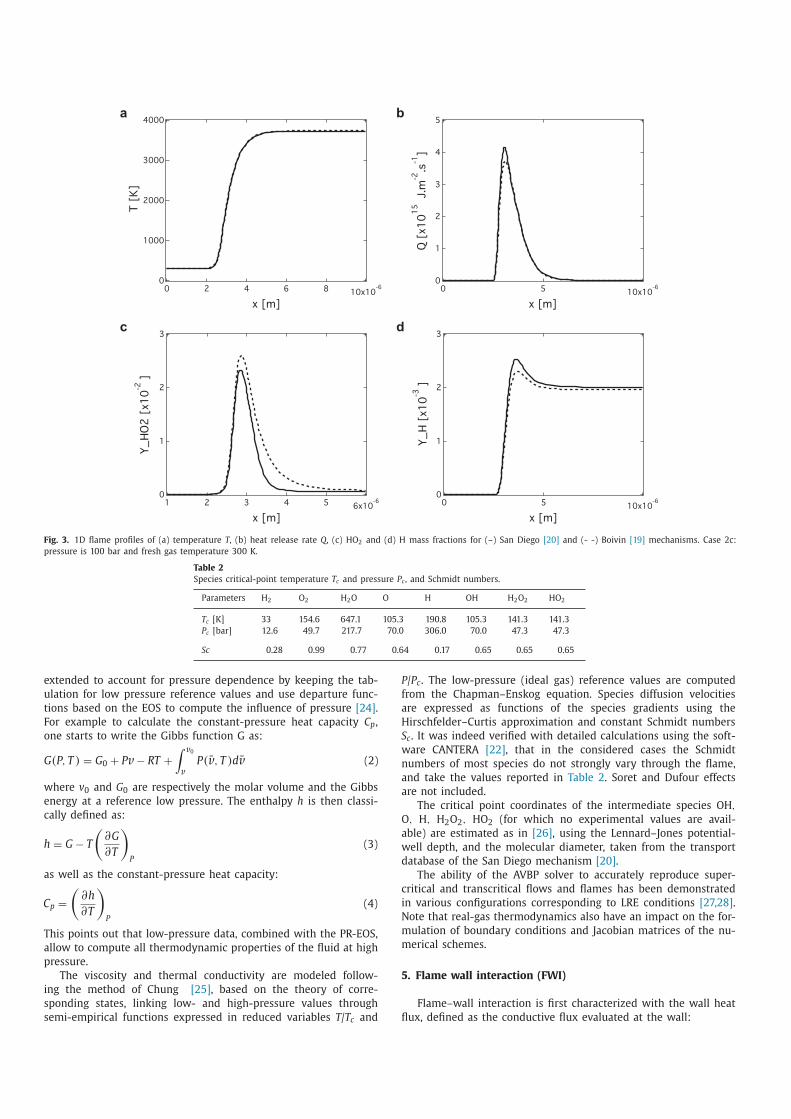
Fig. 3. 1D flame profiles of (a) temperature T , (b) heat release rate Q , (c) HO 2 and (d) H mass fractions for (–) San Diego [20] and (- -) Boivin [19] mechanisms. Case 2c:

pressure is 100 bar and fresh gas temperature 300 K.

Table 2

Species critical-point temperature T c and pressure P c , and Schmidt numbers.

Parameters H 2 O 2 H 2 O O H OH H 2 O 2 HO 2

T c [K] 33 154 .6 647 .1 105 .3 190 .8 105 .3 141 .3 141 .3

P c [bar] 12 .6 49 .7 217 .7 70 .0 306 .0 70 .0 47 .3 47 .3

Sc 0 .28 0 .99 0 .77 0 .64 0 .17 0 .65 0 .65 0 .65

extended to account for pressure dependence by keeping the tab-

ulation for low pressure reference values and use departure func-

tions based on the EOS to compute the influence of pressure [24] .

For example to calculate the constant-pressure heat capacity C p ,

one starts to write the Gibbs function G as:

G (P, T ) = G 0 + P v − RT +

∫ v 0

v P ( ̄v , T ) d ̄v (2)

where v 0 and G 0 are respectively the molar volume and the Gibbs

energy at a reference low pressure. The enthalpy h is then classi-

cally defined as:

h = G − T

(

∂G

∂T

)

P

(3)

as well as the constant-pressure heat capacity:

C p =

(

∂h

∂T

)

P

(4)

This points out that low-pressure data, combined with the PR-EOS,

allow to compute all thermodynamic properties of the fluid at high

pressure.

The viscosity and thermal conductivity are modeled follow-

ing the method of Chung [25] , based on the theory of corre-

sponding states, linking low- and high-pressure values through

semi-empirical functions expressed in reduced variables T / T c and

P / P c . The low-pressure (ideal gas) reference values are computed

from the Chapman–Enskog equation. Species diffusion velocities

are expressed as functions of the species gradients using the

Hirschfelder–Curtis approximation and constant Schmidt numbers

S c . It was indeed verified with detailed calculations using the soft-

ware CANTERA [22] , that in the considered cases the Schmidt

numbers of most species do not strongly vary through the flame,

and take the values reported in Table 2 . Soret and Dufour effects

are not included.

The critical point coordinates of the intermediate species OH ,

O , H , H 2 O 2 , HO 2 (for which no experimental values are avail-

able) are estimated as in [26] , using the Lennard–Jones potential-

well depth, and the molecular diameter, taken from the transport

database of the San Diego mechanism [20] .

The ability of the AVBP solver to accurately reproduce super-

critical and transcritical flows and flames has been demonstrated

in various configurations corresponding to LRE conditions [27,28] .

Note that real-gas thermodynamics also have an impact on the for-

mulation of boundary conditions and Jacobian matrices of the nu-

merical schemes.

5. Flame wall interaction (FWI)

Flame–wall interaction is first characterized with the wall heat

flux, defined as the conductive flux evaluated at the wall:

8w = λw ∂T

∂x

∣

∣

∣

∣

w

(5)

where λw is the thermal conductivity of the fluid evaluated at the

wall. The wall heat flux is stronlgy linked to the flame characteris-

tics: the thermal flame thickness δl is calculated from the temper-

ature gradient:

δl = T b − T u

(∇T ) max (6)

where ( ∇T ) max is the maximum of the temperature gradient. This

flame thickness may be also estimated from the flame parameters

using the diffusive flame thickness δ [7] given by:

δ = λu

ρu C u p S 0 l

(7)

where S 0 l is the laminar flame speed. The laminar flame power Q 0

l is defined as:

Q 0 l = ρu Y u F S

0 l 1H (8)

where Y u F is the fuel mass fraction in unburnt gases and

1H [ J kg −1 ] the heat produced per kilogram of fuel consumed.

The wall heat flux is non-dimensionalized by the flame power

as 8∗w = 8w /Q 0

l , whereas the non-dimensional flame heat release

rate is Q ∗ = Q δ/Q 0 l . In addition, the flame characteristic time τ =

δ/S 0 l is used to non-dimensionalize the time as t ∗ = t/τ, while

space dimensions are non-dimensionalized by the flame thickness

as x ∗ = x/δ. Because of complex chemistry, the definition of the flame posi-

tion is not unique. It can be either located at the maximum of heat

release rate Q max ( x Q max ) or at the maximum of fuel consumption

rate ˙ ω F,max ( x ̇ ω F,max ). Both locations are different and may be used

to define Peclet numbers which characterize the ratio between dif-

fusion and convective characteristic times:

• the heat release Peclet number is

P e = x Q max

δ(9)

• the fuel Peclet number is

P e F = x ̇ ω F,max

δ(10)

Assuming that no reaction occurs at the wall, the temperature

difference T b − T u divided by the flame quenching distance gives

an estimate of the wall temperature gradient. As shown in [5] , this

leads to a simple relationship between the non-dimensional wall

heat flux and the Peclet number (either from the heat release or

fuel consumption) 8∗w ∼ 1 /Pe or, taking into account the wall heat

loss:

8∗w ∼ 1 / (1 + P e ) (11)

Theoretical model: the infinitely fast flame model

The role and importance of the coupling between the solid and

the fluid thermal problems may be understood from the limit case

of infinitely fast flame [17] (IFF), in which the characteristic flame

time scale is negligible compared to the solid conduction time. In

this case the configuration reduces to the simpler problem of two

semi-infinite domains having different tem peratures and a com-

mon contact surface. Solving this classical heat transfer problem

leads to the following expression for the interface temperature:

T IF F w = e w T w + e f T f

e w + e f (12)

where T w ( T f ) is the solid (resp. fluid) temperature, and e w ( e f ) the

solid (resp. fluid) effusivity defined by

e =

√

λρC p (13)

Table 3

Summary of test cases: fresh gases properties at stoichiometry and

compressibility factor calculated using NIST software REFPROP [30] .

Case T u Pressure ρu Compressibility factor

[K] [bar] [kg m −3 ] [Dimensionless]

1 750 1 0.1931 1.0 0 0

2a 1 0.4824 1.0 0 0

2b 300 10 4.8476 0.995

2c 100 48.342 0.998

3 150 100 108.75 0.887

where λ is the heat conductivity, ρ the density and C p the heat

capacity of the solid ( w ) or the fluid ( f ).

Introducing the effusivity ratio parameter κ = e w /e f ,

Eq. (12) can be written

T IF F w = κ T w + T f

κ + 1 (14)

Eq. (14) shows that the interface temperature depends on the pa-

rameter κ: for large values of this ratio, the temperature at the solid/fluid interface stays close to the wall temperature and the

wall may be considered isothermal; on the contrary, low values

of κ allow significant heating of the wall which is then neither

isothermal nor adiabatic. In this last case the resolution of the

unsteady coupled problem is necessary to obtain the correct wall

heat flux.

6. Cases description

Several FWI cases for laminar stoichiometric premixed flames

were performed and are summarized in Table 3 . For all cases, the

initial wall temperature T i w and the fresh gas temperature T u are

taken the same and non-coupled, isothermal simulations (denoted U ) are compared to fluid-thermal solid coupled simulations (de-

noted C ). Case 1 is presented for validation purposes and will be

compared to previous studies [7,10,12] . Cases 2a, 2b and 2c allow

to evaluate the influence of the pressure on FWI and extend the

results to very high pressure. Finally Case 3 corresponds to cryo-

genic flames typical of LREs operating conditions, with very low

fresh gas temperature.

The first effect of pressure increase is the reduction of the flame

thickness, which may be approximated by a power law:

δl (P ) = δl (P 0 ) (

P

P 0

)α

(15)

where P 0 is a reference pressure and α depends on the temper-

ature and the fuel. In the case of stoichiometric hydrogen/oxygen

mixture at 300 K α ∼ −1 . 21 [29] was found, which means that the thermal flame thickness decreases with pressure. This a priori will

have a strong impact on FWI, with an expected increase of wall

heat flux with pressure.

As shown in Table 3 , the fresh gas density ρu increases dras-

tically with increasing pressure and decreasing temperature, up to

200 times (Case 3) higher than the reference Case 2a at ambient

conditions. Looking at the compressibility factor, given by:

Z = P

ρrT (16)

where r is the specific gas constant, the deviation from the ideal

gas law stays close to 1 as long as the temperature remains rela-

tively high. For these cases no strong real gas effects are expected.

With the decrease of the fresh gas temperature, Case 3 leads to a

compressibility factor of 0.887, i.e. presenting significant real gas

effects.

Case T u P T b − T u S 0 l δl δ Q 0

l Mesh cell size

[K] [bar] [K] [m s −1 ] [m] [m] [W m −2 ] [m]

1 750 1 2380 34.27 2.59e −4 1.07e −5 8.66e7 2.0e −6

2a 1 2770 10.76 2.23e −4 6.96e −6 6.87e7 2.0e −6 2b 300 10 3090 12.49 1.21e −5 5.85e −7 8.22e8 2.0e −7 2c 100 3430 9.03 1.18e −6 9.46e −8 6.25e9 1.0e −8

3 150 100 3544 3.96 1.23e −6 5.93e −8 5.47e9 1.0e −8

Table 5

Fluid and wall thermal effusivity, effusivity ratio κ and interface temperature predicted by the IFF

model T IFF w . Thermal effusivity unit is [W m −2 K −1 s −1 / 2 ].

Case T i w Pressure Fluid effusivity e f Wall effusivity e w κ T IFF w [K] [bar] [SI] [SI] [Dimensionless] [K]

1 750 1 6 .09 9280 1524 751.6

2a 1 4 .47 6186 1383 302

2b 300 10 13 .92 6186 4 4 4 307

2c 100 96 .61 6186 64 352.8

3 150 100 93 .62 4914 52.5 216.2

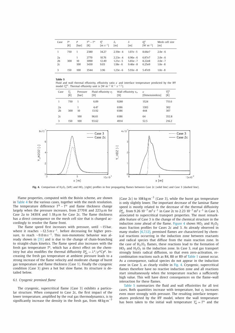
Fig. 4. Comparison of H 2 O 2 (left) and HO 2 (right) profiles in free propagating flames between Case 2c (solid line) and Case 3 (dashed line).

Flame properties, computed with the Boivin scheme, are shown

in Table 4 for the various cases, together with the mesh resolution.

The temperature difference T b − T u and flame thickness change

largely when the pressure increases, from 2770 K and 223 µm for

Case 2a to 3430 K and 1 . 18 µm for Case 2c. The flame thickness

has a direct consequence on the mesh cell size that is changed ac-

cordingly to resolve the flame front.

The flame speed first increases with pressure, until ∼15 bar , where it reaches ∼12 . 5 ms −1 , before decreasing for higher pres-

sure, to reach ∼9 . 0 ms −1 . This non-monotonic behavior was al-

ready shown in [31] and is due to the change of chain-branching

to straight-chain kinetics. The flame speed also increases with the

fresh gas temperature T u , which has a direct effect on the chem-

istry but also modifies the thermal diffusivity D u th

= λu /ρu Cp u . In-

creasing the fresh gas temperature at ambient pressure leads to a

strong increase of the flame velocity and moderate change of burnt

gas temperature and flame thickness (Case 1). Finally the cryogenic

condition (Case 3) gives a hot but slow flame. Its structure is de-

tailed below.

6.1. Cryogenic premixed flame

The cryogenic, supercritical flame (Case 3) exhibits a particu-

lar structure. When compared to Case 2c, the first impact of the

lower temperature, amplified by the real gas thermodynamics, is to

significantly increase the density in the fresh gas, from 48 kg m −3

(Case 2c) to 108 kg m −3 (Case 3), while the burnt gas temperature

is only slightly lower. The important decrease of the laminar flame

speed is mostly related to the decrease of the thermal diffusivity

D u th

, from 9 . 26 10 −7 m 2 s −1 in Case 2c to 2 . 23 10 −7 m 2 s −1 in Case 3,

associated to supercritical transport properties. The most remark-

able feature of Case 3 is the change of the chemical structure in the

induction zone ahead of the flame. Figure 4 shows HO 2 and H 2 O 2

mass fraction profiles for Cases 2c and 3. As already observed in

many studies [6,7,12] , premixed flames are characterized by chem-

ical reactions occurring in the induction zone between reactants

and radical species that diffuse from the main reaction zone. In

the case of H 2 / O 2 flames, these reactions lead to the formation of

HO 2 and H 2 O 2 in the induction zone. In Case 3, real gas transport

strongly limits radical diffusion, so that even zero-activation, re-

combination reactions such as R4, R8 or R9 of Table 1 cannot occur.

As a consequence, radical species do not appear in the induction

zone in Case 3, as clearly visible in Fig. 4 . Cryogenic, supercritical

flames therefore have no reactive induction zone and all reactions

start simultaneously when the temperature reaches a sufficiently

high value. This will have direct consequences on the flame–wall

interaction for these flames.

Table 5 summarizes the fluid and wall effusivities for all test

cases. Both quantities increase with temperature, but e f increases

even more strongly with pressure. The resulting interface temper-

atures predicted by the IFF model, where the wall temperature

has been taken to the initial wall temperature T i w = T u and the

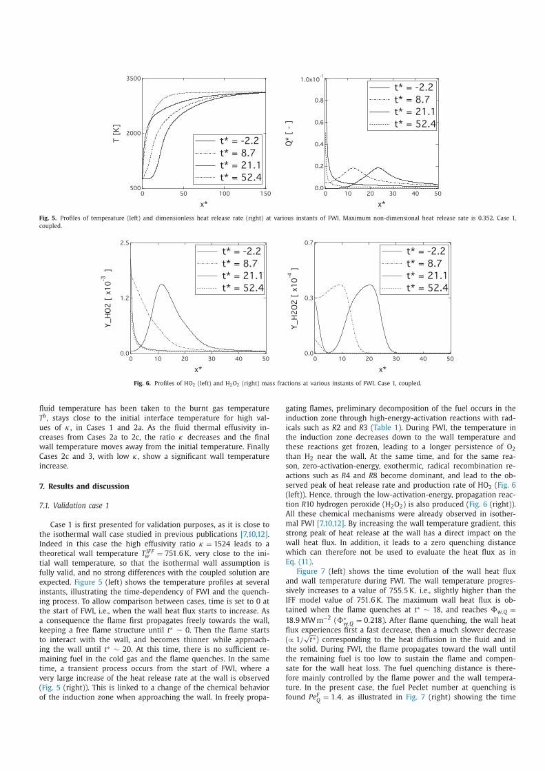
Fig. 5. Profiles of temperature (left) and dimensionless heat release rate (right) at various instants of FWI. Maximum non-dimensional heat release rate is 0.352. Case 1,

coupled.

Fig. 6. Profiles of HO 2 (left) and H 2 O 2 (right) mass fractions at various instants of FWI. Case 1, coupled.

fluid temperature has been taken to the burnt gas temperature

T b , stays close to the initial interface temperature for high val-

ues of κ , in Cases 1 and 2a. As the fluid thermal effusivity in- creases from Cases 2a to 2c, the ratio κ decreases and the final

wall temperature moves away from the initial temperature. Finally

Cases 2c and 3, with low κ , show a significant wall temperature

increase.

7. Results and discussion

7.1. Validation case 1

Case 1 is first presented for validation purposes, as it is close to

the isothermal wall case studied in previous publications [7,10,12] .

Indeed in this case the high effusivity ratio κ = 1524 leads to a

theoretical wall temperature T IF F w = 751 . 6 K , very close to the ini-

tial wall temperature, so that the isothermal wall assumption is

fully valid, and no strong differences with the coupled solution are

expected. Figure 5 (left) shows the temperature profiles at several

instants, illustrating the time-dependency of FWI and the quench-

ing process. To allow comparison between cases, time is set to 0 at

the start of FWI, i.e., when the wall heat flux starts to increase. As

a consequence the flame first propagates freely towards the wall,

keeping a free flame structure until t ∗ ∼ 0. Then the flame starts

to interact with the wall, and becomes thinner while approach-

ing the wall until t ∗ ∼ 20. At this time, there is no sufficient re-

maining fuel in the cold gas and the flame quenches. In the same

time, a transient process occurs from the start of FWI, where a

very large increase of the heat release rate at the wall is observed

( Fig. 5 (right)). This is linked to a change of the chemical behavior

of the induction zone when approaching the wall. In freely propa-

gating flames, preliminary decomposition of the fuel occurs in the

induction zone through high-energy-activation reactions with rad-

icals such as R 2 and R 3 ( Table 1 ). During FWI, the temperature in

the induction zone decreases down to the wall temperature and

these reactions get frozen, leading to a longer persistence of O 2

than H 2 near the wall. At the same time, and for the same rea-

son, zero-activation-energy, exothermic, radical recombination re-

actions such as R 4 and R 8 become dominant, and lead to the ob-

served peak of heat release rate and production rate of HO 2 ( Fig. 6

(left)). Hence, through the low-activation-energy, propagation reac-

tion R 10 hydrogen peroxide ( H 2 O 2 ) is also produced ( Fig. 6 (right)).

All these chemical mechanisms were already observed in isother-

mal FWI [7,10,12] . By increasing the wall temperature gradient, this

strong peak of heat release at the wall has a direct impact on the

wall heat flux. In addition, it leads to a zero quenching distance

which can therefore not be used to evaluate the heat flux as in

Eq. (11) .

Figure 7 (left) shows the time evolution of the wall heat flux

and wall temperature during FWI. The wall temperature progres-

sively increases to a value of 755 . 5 K , i.e., slightly higher than the

IFF model value of 751 . 6 K . The maximum wall heat flux is ob-

tained when the flame quenches at t ∗ ∼ 18, and reaches 8w,Q =

18 . 9 MWm −2 ( 8∗

w,Q = 0 . 218 ). After flame quenching, the wall heat

flux experiences first a fast decrease, then a much slower decrease

( ∝ 1 / √ t ∗) corresponding to the heat diffusion in the fluid and in

the solid. During FWI, the flame propagates toward the wall until

the remaining fuel is too low to sustain the flame and compen-

sate for the wall heat loss. The fuel quenching distance is there-

fore mainly controlled by the flame power and the wall tempera-

ture. In the present case, the fuel Peclet number at quenching is

found Pe F Q = 1 . 4 , as illustrated in Fig. 7 (right) showing the time

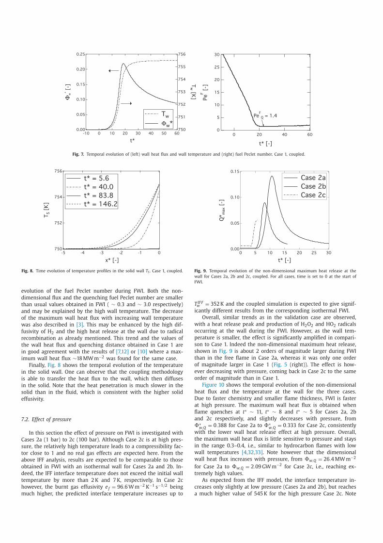
Fig. 7. Temporal evolution of (left) wall heat flux and wall temperature and (right) fuel Peclet number. Case 1, coupled.

Fig. 8. Time evolution of temperature profiles in the solid wall T S . Case 1, coupled.

evolution of the fuel Peclet number during FWI. Both the non-

dimensional flux and the quenching fuel Peclet number are smaller

than usual values obtained in FWI ( ∼ 0.3 and ∼ 3.0 respectively)

and may be explained by the high wall temperature. The decrease

of the maximum wall heat flux with increasing wall temperature

was also described in [3] . This may be enhanced by the high dif-

fusivity of H 2 and the high heat release at the wall due to radical

recombination as already mentioned. This trend and the values of

the wall heat flux and quenching distance obtained in Case 1 are

in good agreement with the results of [7,12] or [10] where a max-

imum wall heat flux ∼18 MW m −2 was found for the same case.

Finally, Fig. 8 shows the temporal evolution of the temperature

in the solid wall. One can observe that the coupling methodology

is able to transfer the heat flux to the wall, which then diffuses

in the solid. Note that the heat penetration is much slower in the

solid than in the fluid, which is consistent with the higher solid

effusivity.

7.2. Effect of pressure

In this section the effect of pressure on FWI is investigated with

Cases 2a (1 bar) to 2c (100 bar). Although Case 2c is at high pres-

sure, the relatively high temperature leads to a compressibility fac-

tor close to 1 and no real gas effects are expected here. From the

above IFF analysis, results are expected to be comparable to those

obtained in FWI with an isothermal wall for Cases 2a and 2b. In-

deed, the IFF interface temperature does not exceed the initial wall

temperature by more than 2 K and 7 K , respectively. In Case 2c

however, the burnt gas effusivity e f = 96 . 6 W m −2 K −1 s −1 / 2 being

much higher, the predicted interface temperature increases up to

Fig. 9. Temporal evolution of the non-dimensional maximum heat release at the

wall for Cases 2a, 2b and 2c, coupled. For all cases, time is set to 0 at the start of

FWI.

T IF F w = 352 K and the coupled simulation is expected to give signif-

icantly different results from the corresponding isothermal FWI.

Overall, similar trends as in the validation case are observed,

with a heat release peak and production of H 2 O 2 and HO 2 radicals

occurring at the wall during the FWI. However, as the wall tem-

perature is smaller, the effect is significantly amplified in compari-

son to Case 1. Indeed the non-dimensional maximum heat release,

shown in Fig. 9 is about 2 orders of magnitude larger during FWI

than in the free flame in Case 2a, whereas it was only one order

of magnitude larger in Case 1 ( Fig. 5 (right)). The effect is how-

ever decreasing with pressure, coming back in Case 2c to the same

order of magnitude than in Case 1.

Figure 10 shows the temporal evolution of the non-dimensional

heat flux and the temperature at the wall for the three cases.

Due to faster chemistry and smaller flame thickness, FWI is faster

at high pressure. The maximum wall heat flux is obtained when

flame quenches at t ∗ ∼ 11, t ∗ ∼ 8 and t ∗ ∼ 5 for Cases 2a, 2b

and 2c respectively, and slightly decreases with pressure, from

8∗w,Q = 0 . 388 for Case 2a to 8∗

w,Q = 0 . 333 for Case 2c, consistently

with the lower wall heat release effect at high pressure. Overall,

the maximum wall heat flux is little sensitive to pressure and stays

in the range 0.3–0.4, i.e., similar to hydrocarbon flames with low

wall temperatures [4,32,33] . Note however that the dimensional

wall heat flux increases with pressure, from 8w,Q = 26 . 4 MW m −2

for Case 2a to 8w,Q = 2 . 09 GW m −2 for Case 2c, i.e., reaching ex-

tremely high values.

As expected from the IFF model, the interface temperature in-

creases only slightly at low pressure (Cases 2a and 2b), but reaches

a much higher value of 545 K for the high pressure Case 2c. Note

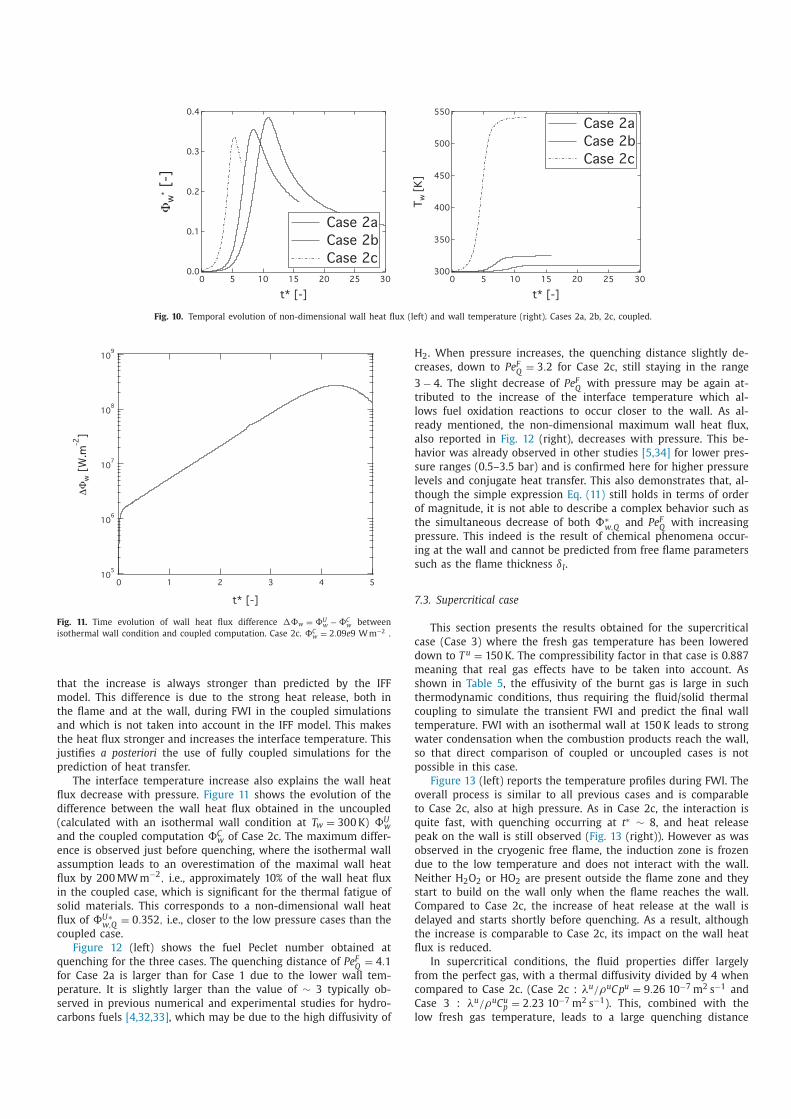
Fig. 10. Temporal evolution of non-dimensional wall heat flux (left) and wall temperature (right). Cases 2a, 2b, 2c, coupled.

Fig. 11. Time evolution of wall heat flux difference 18w = 8U w − 8C

w between

isothermal wall condition and coupled computation. Case 2c. 8C w = 2 . 09 e 9 W m −2 .

that the increase is always stronger than predicted by the IFF

model. This difference is due to the strong heat release, both in

the flame and at the wall, during FWI in the coupled simulations

and which is not taken into account in the IFF model. This makes

the heat flux stronger and increases the interface temperature. This

justifies a posteriori the use of fully coupled simulations for the

prediction of heat transfer.

The interface temperature increase also explains the wall heat

flux decrease with pressure. Figure 11 shows the evolution of the

difference between the wall heat flux obtained in the uncoupled

(calculated with an isothermal wall condition at T w = 300 K ) 8U w

and the coupled computation 8C w of Case 2c. The maximum differ-

ence is observed just before quenching, where the isothermal wall

assumption leads to an overestimation of the maximal wall heat

flux by 200 MW m −2

, i.e., approximately 10% of the wall heat flux

in the coupled case, which is significant for the thermal fatigue of

solid materials. This corresponds to a non-dimensional wall heat

flux of 8U∗w,Q = 0 . 352 , i.e., closer to the low pressure cases than the

coupled case.

Figure 12 (left) shows the fuel Peclet number obtained at

quenching for the three cases. The quenching distance of Pe F Q = 4 . 1

for Case 2a is larger than for Case 1 due to the lower wall tem-

perature. It is slightly larger than the value of ∼ 3 typically ob-

served in previous numerical and experimental studies for hydro-

carbons fuels [4,32,33] , which may be due to the high diffusivity of

H 2 . When pressure increases, the quenching distance slightly de-

creases, down to Pe F Q = 3 . 2 for Case 2c, still staying in the range

3 − 4 . The slight decrease of Pe F Q with pressure may be again at-

tributed to the increase of the interface temperature which al-

lows fuel oxidation reactions to occur closer to the wall. As al-

ready mentioned, the non-dimensional maximum wall heat flux,

also reported in Fig. 12 (right), decreases with pressure. This be-

havior was already observed in other studies [5,34] for lower pres-

sure ranges (0.5–3.5 bar) and is confirmed here for higher pressure

levels and conjugate heat transfer. This also demonstrates that, al-

though the simple expression Eq. (11) still holds in terms of order

of magnitude, it is not able to describe a complex behavior such as

the simultaneous decrease of both 8∗w,Q and Pe

F Q with increasing

pressure. This indeed is the result of chemical phenomena occur-

ing at the wall and cannot be predicted from free flame parameters

such as the flame thickness δl .

7.3. Supercritical case

This section presents the results obtained for the supercritical

case (Case 3) where the fresh gas temperature has been lowered

down to T u = 150 K . The compressibility factor in that case is 0.887

meaning that real gas effects have to be taken into account. As

shown in Table 5 , the effusivity of the burnt gas is large in such

thermodynamic conditions, thus requiring the fluid/solid thermal

coupling to simulate the transient FWI and predict the final wall

temperature. FWI with an isothermal wall at 150 K leads to strong

water condensation when the combustion products reach the wall,

so that direct comparison of coupled or uncoupled cases is not

possible in this case.

Figure 13 (left) reports the temperature profiles during FWI. The

overall process is similar to all previous cases and is comparable

to Case 2c, also at high pressure. As in Case 2c, the interaction is

quite fast, with quenching occurring at t ∗ ∼ 8, and heat release

peak on the wall is still observed ( Fig. 13 (right)). However as was

observed in the cryogenic free flame, the induction zone is frozen

due to the low temperature and does not interact with the wall.

Neither H 2 O 2 or HO 2 are present outside the flame zone and they

start to build on the wall only when the flame reaches the wall.

Compared to Case 2c, the increase of heat release at the wall is

delayed and starts shortly before quenching. As a result, although

the increase is comparable to Case 2c, its impact on the wall heat

flux is reduced.

In supercritical conditions, the fluid properties differ largely

from the perfect gas, with a thermal diffusivity divided by 4 when

compared to Case 2c. (Case 2c : λu /ρu Cp u = 9 . 26 10 −7 m 2 s −1 and

Case 3 : λu /ρu C u p = 2 . 23 10 −7 m 2 s −1 ). This, combined with the

low fresh gas temperature, leads to a large quenching distance

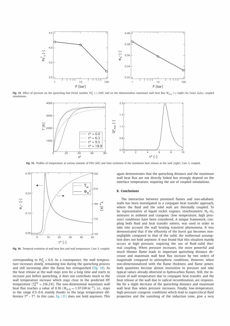
Fig. 12. Effect of pressure on the quenching fuel Peclet number Pe F Q ( ◦) (left) and on the dimensionless maximum wall heat flux 8∗w,Q ( ◦) (right) for Cases 2a,b,c, coupled

simulations.

Fig. 13. Profiles of temperature at various instants of FWI (left) and time evolution of the maximum heat release at the wall (right). Case 3, coupled.

Fig. 14. Temporal evolution of wall heat flux and wall temperature. Case 3, coupled.

corresponding to Pe F Q = 6 . 0 . As a consequence, the wall tempera-

ture increases slowly, remaining low during the quenching process

and still increasing after the flame has extinguished ( Fig. 14 ). As

the heat release at the wall stays zero for a long time and starts to

increase just before quenching, it does not contribute much to the

wall temperature increase which stays close to the predicted IFF

temperature ( T IF F w = 216 . 2 K ). The non-dimensional maximum wall

heat flux reaches a value of 0.36 ( 8w,Q = 1 . 97 GW m −2 ), i.e., stays

in the range 0.3–0.4, mainly thanks to the large temperature dif-

ference T b − T u . In this case, Eq. (11) does not hold anymore. This

again demonstrates that the quenching distance and the maximum

wall heat flux are not directly linked but strongly depend on the

interface temperature, requiring the use of coupled simulations.

8. Conclusions

The interaction between premixed flames and non-adiabatic

walls has been investigated in a conjugate heat transfer approach,

where the fluid and the solid wall are thermally coupled. To

be representative of liquid rocket engines, stoichiometric H 2 –O 2

mixtures in ambient and cryogenic (low temperature, high pres-

sure) conditions have been considered. A unique framework, cou-

pling both fluid and heat transfer solvers, was used in order to

take into account the wall heating transient phenomena. It was

demonstrated that if the effusivity of the burnt gas becomes non-

negligible compared to that of the solid, the isothermal assump-

tion does not hold anymore. It was found that this situation mainly

occurs at high pressure, requiring the use of fluid–solid ther-

mal coupling. When pressure increases, the more powerful and

much thinner flame leads to important quenching distance de-

crease and maximum wall heat flux increase by two orders of

magnitude compared to atmospheric conditions. However, when

non-dimensionalized with the flame thickness and flame power,

both quantities become almost insensitive to pressure and take

typical values already observed in hydrocarbon flames. Still, the in-

crease of wall temperature due to conjugate heat transfer, and the

heat release at the wall due to radical recombination, are responsi-

ble for a slight decrease of the quenching distance and maximum

wall heat flux when pressure increases. Finally, low-temperature,

high-pressure cryogenic conditions which lead to supercritical fluid

properties and the vanishing of the induction zone, give a very

large quenching distance. However the non-dimensional maximum

wall heat flux stays comparable to the previous cases. In this case

also, significant impact of the conjugate heat transfer is observed

and requires fluid–solid thermal coupling to describe accurately

the wall temperature and the flame behavior. These findings may

have important implications for flame stabilization and thermal fa-

tigue in practical systems such as liquid rocket engine injectors.

The demonstrated feasibility and relevance of thermally coupled

fluid–solid simulations allows to remove the uncertainty about the

wall thermal conditions and improve the prediction and design of

optimum burner geometries.

Supplementary material

Supplementary material associated with this article can be

found, in the online version, at 10.1016/j.combustflame.2016.01.

004 .

References

[1] G. Bruneaux , T. Poinsot , J.H. Ferziger , Premixed flame–wall interaction in a tur- bulent channel flow: budget for the flame surface density evolution equation and modelling, J. Fluid Mech. 349 (1997) 191–219 .

[2] T. Poinsot , D. Haworth , G. Bruneaux , Direct simulation and modelling of flame–wall interaction for premixed turbulent combustion, Combust. Flame 95 (1/2) (1993) 118–133 .

[3] O.A. Ezekoye , R. Greif , D. Lee , Increased surface temperatureeffects on wall heat transfer during unsteady flame quenching, Symp. (Int.) Combust. 24 (1) (1992) 1465–1472 .

[4] J.H. Lu , O. Ezekoye , R. Greif , F. Sawyer , Unsteady heat transfer during side wall quenching of a laminar flame, Symp. (Int.) Combust. 23 (1) (1990) 4 41–4 46 .

[5] B. Boust , J. Sotton , S. Labuda , M. Bellenoue , A thermal formulation for sin- gle-wall quenching of transient laminar flames, Combust. Flame 149 (3) (2007) 286–294 .

[6] C.K. Westbrook , A .A . Adamczyk , G.A . Lavoie , A numerical study of laminar flame wall quenching., Combust. Flame 40 (1981) 81–99 .

[7] F. Dabireau , B. Cuenot , O. Vermorel , T. Poinsot , Interaction of H 2 /O 2 flames with inert walls, Combust. Flame 135 (1–2) (2003) 123–133 .

[8] A. Delataillade , F. Dabireau , B. Cuenot , T. Poinsot , Flame/wall interaction and maximum heat wall fluxes in diffusion burners, Proc. Combust. Inst. 29 (2002) 775–780 .

[9] P. Popp , M. Baum , An analysis of wall heat fluxes, reaction mechanisms and unburnt hydrocarbons during the head-on quenching of a laminar methane flame, Combust. Flame 108 (3) (1997) 327–348 .

[10] R. Owston , V. Magi , J. Abraham , Interactions of hydrogens flames with walls: influence of wall temperature, pressure, equivalence ratio and diluents, Int. J. Hydrogen Energy 32 (2007) 2094–2104 .

[11] T.K. Kim , D.H. Lee , S. Kwon , Effects of thermal and chemical surface–flame in- teraction on flame quenching, Combust. Flame 146 (2006) 19–28 .

[12] A. Gruber , R. Sankaran , E.R. Hawkes , J. Chen , Turbulent flame–wall interaction: a direct numerical simulation study, J. Fluid Mech. 658 (2010) 5–32 .

[13] F. Duchaine , A. Corpron , L. Pons , V. Moureau , F. Nicoud , T. Poinsot , Develop- ment and assessment of a coupled strategy for conjugate heat transfer with large eddy simulation: application to a cooled turbine blade, Int. J. Heat Fluid Flow 30 (6) (2009) 1129–1141 .

[14] L. Quartapelle , V. et Selmin , High-order Taylor-Galerkin methods for nonlinear multidimensional problems, Finite Elements in Fluids 76 (90) (1993) 46 .

[15] O. Colin , M. Rudgyard , Development of high-order Taylor–Galerkin schemes for LES, J. Comput. Phys. 162 (2) (20 0 0) 338–371 .

[16] S. Buis , A. Piacentini , D. Déclat , PALM: a computational framework for as- sembling high performance computing applications, Concurr. Comput. 18 (2) (2005) 231–245 .

[17] F. Duchaine , S. Mendez , F. Nicoud , A. Corpron , V. Moureau , T. Poinsot , Conju- gate heat transfer with large eddy simulation application to gas turbine com- ponents, Comptes Rendus Acad. Sci. Mécanique 337 (6-7) (2009) 550–561 .

[18] T. Poinsot , T. Echekki , M.G. Mungal , A study of the laminar flame tip and im- plications for premixed turbulent combustion, Combust. Sci. Technol. 81 (1-3) (1992) 45–73 .

[19] P. Boivin , C. Jiménez , A. Sanchez , F. Williams , An explicit reduced mechanism

for H 2 –air combustion, Proc. Combust. Inst. 33 (1) (2011) 517–523 . [20] P. Saxena , F. Williams , Testing a small detailed chemical-kinetic mechanism

for the combustion of hydrogen and carbon monoxide., Combust. Flame 145 (2006) 316–323 .

[21] A . Sanchez , F.A . Williams , Recent advances in understanding of flammability characteristics of hydrogen, Prog. Energy Combust. Sci. 41 (2013) 1–55 .

[22] D.G. Goodwin , CANTERA: An open-source, object-oriented software suite for combustion, NSF Workshop on Cyber-based Combustion Science, National Sci- ence Foundation, NSF Headquarters, Arlington, VA (2006) .

[23] D.Y. Peng , D.B. Robinson , A new two-constant equation of state, Ind. Eng. Chem. Fundam. 15 (1) (1976) 59–64 .

[24] B.E. Poling , J.M. Prausnitz , J.P. O’Connell , The properties of gases and liquids, 5th ed., McGraw-Hill, 2001 .

[25] T.-H. Chung , L.L. Lee , K.E. Starling , Application of kinetic gas theories and mul- tiparameter correlation for prediction of dilute gas viscosity and thermal con- ductivity, Ind. Eng. Chem. Fundam. 23 (1984) 8–13 .

[26] V. Giovangigli , L. Matuszewski , F. Dupoirieux , Detailed modeling of planar tran- scritical H 2 -O 2 –N 2 flames, Combust. Theory Model. 15 (2) (2011) 141–182 .

[27] A. Ruiz , L. Selle , Simulation of a turbulent supercritical hydrogen/oxygen flow

behind a splitter plate: cold flow and flame stabilization, Seventh Mediter- ranean Combustion Symposium (2011) .

[28] T. Schmitt , L. Selle , A. Ruiz , B. Cuenot , Large-eddy simulation of supercritical–pressure round jets, AIAA J. 48 (9) (2010) 2133–2144 .

[29] J. Warnatz , Concentration-, pressure-, and temperature-dependence of the flame velocity in hydrogen-oxygen-nitrogen mixtures, Combust. Sci. Technol. 26 (1981) 203–213 .

[30] E. Lemmon , M. Huber , M. McLinden , NIST standard reference database 23: ref- erence fluid thermodynamic and transport properties-REFPROP, Version 8.0, Technical Report, National Institute of Standards and Technology, Standard Ref- erence Data Program, Gaithersburg, MD, 2007 .

[31] M. Kuznetsov , R. Redlinger , W. Breitung , J. Grune , A. Friedrich , N. Ichikawa , Laminar burning velocities of hydrogen–oxygen-steam mixtures at elevated temperatures and pressures, Proc. Combust. Inst. 33 (2011) 895–903 .

[32] W.M. Huang , S.R. Vosen , R. Greif , Heat transfer during laminar flame quench- ing, effect of fuels, Symp. (Int.) Combust. 21 (1) (1986) 1853–1860 .

[33] S.R. Vosen , R. Greif , C.K. Westbrook , Unsteady heat transfer during laminar flame quenching., Symp. (Int.) Combust. 20 (1) (1984) 76–83 .

[34] J. Sotton , B. Boust , S. Labuda , M. Bellenoue , Head-on quenching of transient laminar flame: heat flux and quenching distance measurements, Combust. Sci. Technol. 177 (7) (2005) 1305–1322 .