HAL Id: hal-01373784https://hal.archives-ouvertes.fr/hal-01373784

Submitted on 29 Sep 2016

HAL is a multi-disciplinary open accessarchive for the deposit and dissemination of sci-entific research documents, whether they are pub-lished or not. The documents may come fromteaching and research institutions in France orabroad, or from public or private research centers.

L’archive ouverte pluridisciplinaire HAL, estdestinée au dépôt et à la diffusion de documentsscientifiques de niveau recherche, publiés ou non,émanant des établissements d’enseignement et derecherche français ou étrangers, des laboratoirespublics ou privés.

Fast Single Image Super-Resolution Using a NewAnalytical Solution for l2–l2 Problems

Ningning Zhao, Qi Wei, Adrian Basarab, Nicolas Dobigeon, Denis Kouamé,Jean-Yves Tourneret

To cite this version:Ningning Zhao, Qi Wei, Adrian Basarab, Nicolas Dobigeon, Denis Kouamé, et al.. Fast Single ImageSuper-Resolution Using a New Analytical Solution for l2–l2 Problems. IEEE Transactions on ImageProcessing, Institute of Electrical and Electronics Engineers, 2016, vol. 25 (n° 8), pp. 3683-3697.�10.1109/TIP.2016.2567075�. �hal-01373784�

Open Archive TOULOUSE Archive Ouverte (OATAO) OATAO is an open access repository that collects the work of Toulouse researchers and makes it freely available over the web where possible.

This is an author-deposited version published in : http://oatao.univ-toulouse.fr/ Eprints ID : 16140

To link to this article : DOI : 10.1109/TIP.2016.2567075URL : http://dx.doi.org/10.1109/TIP.2016.2567075

To cite this version : Zhao, Ningning and Wei, Qi and Basarab, Adrian and Dobigeon, Nicolas and Kouamé, Denis and Tourneret, Jean-Yves Fast Single Image Super-Resolution Using a New Analytical Solution for l2–l2 Problems. (2016) IEEE Transactions on Image Processing, vol. 25 (n° 8). pp. 3683-3697. ISSN 1057-7149

Any correspondence concerning this service should be sent to the repository

administrator: staff-oatao@listes-diff.inp-toulouse.fr

Fast Single Image Super-Resolution Using a NewAnalytical Solution for ℓ2–ℓ2 Problems

Ningning Zhao, Student Member, IEEE, Qi Wei, Student Member, IEEE, Adrian Basarab, Member, IEEE,Nicolas Dobigeon, Senior Member, IEEE, Denis Kouamé, Member, IEEE,

and Jean-Yves Tourneret, Senior Member, IEEE

Abstract—This paper addresses the problem of single imagesuper-resolution (SR), which consists of recovering a high-resolution image from its blurred, decimated, and noisy version.The existing algorithms for single image SR use different strate-gies to handle the decimation and blurring operators. In additionto the traditional first-order gradient methods, recent techniquesinvestigate splitting-based methods dividing the SR problem intoup-sampling and deconvolution steps that can be easily solved.Instead of following this splitting strategy, we propose to deal withthe decimation and blurring operators simultaneously by takingadvantage of their particular properties in the frequency domain,leading to a new fast SR approach. Specifically, an analyticalsolution is derived and implemented efficiently for the Gaussianprior or any other regularization that can be formulated intoan ℓ2-regularized quadratic model, i.e., an ℓ2–ℓ2 optimizationproblem. The flexibility of the proposed SR scheme is shownthrough the use of various priors/regularizations, ranging fromgeneric image priors to learning-based approaches. In the case ofnon-Gaussian priors, we show how the analytical solution derivedfrom the Gaussian case can be embedded into traditional splittingframeworks, allowing the computation cost of existing algorithmsto be decreased significantly. Simulation results conducted onseveral images with different priors illustrate the effectiveness ofour fast SR approach compared with existing techniques.

Index Terms—Single image super-resolution, deconvolution,decimation, block circulant matrix, variable splitting basedalgorithms.

I. INTRODUCTION

S INGLE image super-resolution (SR), also known as imagescaling up or image enhancement, aims at estimating

a high-resolution (HR) image from a low-resolution (LR)observed image [1]. This resolution enhancement problem isstill an ongoing research problem with applications in various

N. Zhao, N. Dobigeon, and J.-Y. Tourneret are with the Univer-sity of Toulouse, Toulouse 31071, France (e-mail: nzhao@enseeiht.fr;nicolas.dobigeon@enseeiht.fr; jean-yves.tourneret@enseeiht.fr).Q. Wei is with the Department of Engineering, University of Cambridge,

Cambridge CB21PZ, U.K. (e-mail: qw245@cam.ac.uk).A. Basarab and D. Kouamé are with the Institut de Recherche en Informa-

tique de Toulouse, University of Toulouse, Toulouse F-31062, France (e-mail:adrian.basarab@irit.fr; denis.kouame@irit.fr).

Digital Object Identifier 10.1109/TIP.2016.2567075

fields, based on remote sensing [2], video surveillance [3],hyperspectral [4], microwave [5] or medical imaging [6].

The methods dedicated to single image SR can be classi-fied into three categories [7]–[9]. The first category includesthe interpolation based algorithms based on nearest neighborinterpolation, bicubic interpolation [10] or adaptive inter-polation techniques [11], [12]. Despite their simplicity andeasy implementation, it is well-known that these algorithmsgenerally over-smooth the high frequency details. The secondtype of methods consider learning-based (or example-based)algorithms that learn the relations between LR and HR imagepatches from a given database [7], [13]–[16]. Note that theeffectiveness of the learning-based algorithms highly dependson the training image database and that these algorithms havegenerally a high computational complexity. Reconstruction-based approaches that are considered in this paper belong tothe third category of SR approaches [8], [9], [17], [18]. Theseapproaches formulate the image SR as a reconstruction prob-lem, either by incorporating priors in a Bayesian frameworkor by introducing regularizations into an inverse problem.

Existing reconstruction-based techniques used to solve thesingle image SR include the first order gradient-based meth-ods [7]–[9], [17], the iterative shrinkage thresholding-basedalgorithms [19] (also called forward-backward algorithms),proximal gradient algorithms and other variable splitting algo-rithms that rely on the augmented Lagrangian (AL) scheme.The AL-based algorithms include the alternating directionmethod of multipliers (ADMM) [2], [6], [18], [20], splitBregman (SB) methods [5] (known to be equivalent to ADMMin certain conditions [21]) and their variants. Particularly, Nget al. [18] proposed an ADMM-based algorithm to solve aTV-regularized single image SR problem, where the decima-tion and blurring operators are split and solved iteratively.Due to this splitting, the cumbersome SR problem can bedecomposed into an up-sampling problem and a deconvolutionproblem, that can be both solved efficiently. Yanovsky et

al. [5] proposed to solve the same problem with an SplitBregman (SB) algorithm. However, the decimation operatorwas handled through a gradient descent method integrated inthe SB framework. Sun et al. [8], [17] proposed a gradientprofile prior and formulated the single image SR problemas an ℓ2-regularized optimization problem, further solvedwith the gradient descent method. Yang et al. [7] proposeda learning-based algorithm for single image SR by seek-ing a sparse representation using the patches of LR and

HR images, followed by back-projection through a gradientdescent method.

This paper aims at reducing the computational cost ofthese SR methods by proposing a new approach handling thedecimation and blurring operators simultaneously by explor-ing their intrinsic properties in the frequency domain. Itis interesting to note that similar properties were exploredin [22] and [23] for multi-frame SR. However, the implemen-tation of the matrix inversions proposed in [22] and [23] areless efficient than those proposed in this work, as it will bedemonstrated in the complexity analysis conducted in SectionIII. More precisely, this paper derives a closed-form expressionof the solution associated with the ℓ2-penalized least-squaresSR problem, when the observed LR image is assumed to be anoisy, subsampled and blurred version of the HR image witha spatially invariant blur. This model, referred to as ℓ2–ℓ2 inwhat follows, underlies the restoration of an image contami-nated by additive Gaussian noise and has been used intensivelyfor the single image SR problem, see, e.g., [7], [8], [24].The proposed solution is shown to be easily embeddable intoan AL framework to handle non-Gaussian priors (i.e., non-ℓ2regularizations), which significantly lightens the computationalburdens of several existing SR algorithms.

The remainder of the paper is organized as follows.Section II formulates the single image SR problem as anoptimization problem. In Section III, we study the propertiesof the down-sampling and blurring operators in the frequencydomain and introduce a fast SR scheme based on an ana-lytical solution for the ℓ2–ℓ2 model that can be formulatedin the image or gradient domains. Section IV generalizes theproposed fast SR scheme to more complex regularizations inimage or transformed domains. Various experiments presentedin Section V demonstrate the efficiency of the proposed fastsingle image SR scheme. Conclusions and perspectives arefinally reported in Section VI.

II. IMAGE SUPER-RESOLUTION FORMULATION

A. Model of Image Formation

In the single image SR problem, the observed LR image ismodeled as a noisy version of the blurred and decimated HRimage to be estimated as follows,

y = SHx + n (1)

where the vector y ∈ RNl ×1(Nl = ml × nl ) denotes the LRobserved image and x ∈ RNh ×1(Nh = mh × nh) is thevectorized HR image to be estimated, with Nh > Nl . Thevectors y and x are obtained by stacking the correspondingimages (LR image ∈ R

ml×nl and HR image ∈ Rmh×nh ) into

column vectors in a lexicographic order. Note that the vectorn ∈ RNl ×1 is an independent identically distributed (i.i.d.)additive white Gaussian noise (AWGN) and that the matricesS ∈ RNl×Nh and H ∈ RNh×Nh represent the decimationand the blurring/convolution operations respectively. Morespecifically,H is a block circulant matrix with circulant blocks,which corresponds to cyclic convolution boundaries, and leftmultiplying by S performs down-sampling with an integerfactor d (d = dr × dc), i.e., Nh = Nl × d . The decimationfactors dr and dc represent the numbers of discarded rows

Fig. 1. Effect of the up-sampling matrix SH on a 3 × 3 image and of thedown-sampling matrix S on the corresponding 9 × 9 image (whose scale upfactor equals 3).

and columns from the input images satisfying the followingrelationships mh = ml × dr and nh = nl × dc. Note thatthe image formation model (1) has been widely considered insingle image SR problems, see, e.g., [7], [8], [17], [18], [25].

We introduce two additional basic assumptions about theblurring and decimation operators. These assumptions havebeen widely used for image deconvolution or image SRproblems (see, e.g., [7], [16], [26], [27]) and are necessaryfor the proposed fast SR framework.

Assumption 1: The blurring matrix H is the matrix repre-

sentation of the cyclic convolution operator, i.e., H is a block

circulant matrix with circulant blocks (BCCB).

This assumption has been widely used in the image process-ing literature [22], [23], [28]. It is satisfied provided the blur-ring kernel is shift-invariant and the boundary conditions makethe convolution operator periodic. Note that the BCCB matrixassumption does not depend on the shape of the blurringkernel, i.e., it is satisfied for any kind of blurring, includingmotion blur, out-of-focus blur, atmospheric turbulence, etc.Using the cyclic convolution assumption, the blurring matrixand its conjugate transpose can be decomposed as

H = FH3F (2)

HH = FH3

HF (3)

where the matrices F and FH are associated with the Fourierand inverse Fourier transforms (satisfying FFH = FHF = INh )and 3 = diag{Fh} ∈ CNh×Nh is a diagonal matrix, whosediagonal elements are the Fourier coefficients of the firstcolumn of the blurring matrix H, denoted as h. Using thedecompositions (2) and (3), the blurring operator Hx and itsconjugate HHx can be efficiently computed in the frequencydomain, see, e.g., [26], [29], [30].

Assumption 2: The decimation matrix S ∈ RNl×Nh is a

down-sampling operator, while its conjugate transpose SH ∈

RNh×Nl interpolates the decimated image with zeros.

Once again, numerous research works have used thisassumption [7], [16], [22], [23]. Fig. 1 shows a toy examplehighlighting the roles of the decimation matrix S and itsconjugate transpose SH . The decimation matrix satisfies therelationship SSH = INl . Denoting S , SHS, multiplyingan image by S can be achieved by making an entry-wisemultiplication with an Nh × Nh mask having ones at thesampled positions and zeros elsewhere.

B. Problem Formulation

Similar to traditional image reconstruction problems, theestimation of an HR image from the observation of an

LR image is not invertible, leading to an ill-posed problem.This ill-posedness is classically overcome by incorporatingsome appropriate prior information or regularization term.The regularization term can be chosen from a specific taskof interest, the information resulting from previous experi-ments or from a perceptual view on the constraints affectingthe unknown model parameters [31], [32]. Various priorsor regularizations have already been advocated to regular-ize the image SR problem include: (i) traditional genericimage priors such as Tikhonov [24], [33], [34], the totalvariation (TV) [18], [20], [35] and the sparsity in trans-formed domains [36]–[39], (ii) more recently proposed imageregularizations such as the gradient profile prior [8], [9],[17] or Fattal’s edge statistics [40] and (iii) learning-basedpriors [41], [42]. The fast approach proposed in the nextsection is shown to be adapted to many of the existingregularization terms. Note that proposing new regularizationterms with improved SR performance is out of the scope ofthis paper.

Assuming that the noise n in (1) is AWGN and incorporat-ing a proper regularization to the target image x, the maximuma posteriori (MAP) estimator of x for the single image SR canbe obtained by solving the following optimization problem

minx

1

2‖y − SHx‖22︸ ︷︷ ︸

data fidelity

+ τ φ(Ax)︸ ︷︷ ︸

regularization

(4)

where ‖y − SHx‖22 is a data fidelity term associated withthe model likelihood and φ(Ax) is related to the image priorinformation and is referred to as regularization or penalty [43].Note that the matrix A can be the identity matrix when theregularization is imposed on the SR image itself, the gradientoperator, any orthogonal matrix or normalized tight frame,depending on the addressed application and the properties ofthe target image. The role of the regularization parameter τ

is to weight the importance of the regularization term withrespect to (w.r.t.) the data fidelity term. The next sectionderives a closed-form solution of the problem (4) for aquadratic regularizing operator φ(·) when the assumptions 1and 2 hold.

III. PROPOSED FAST SUPER-RESOLUTION

USING AN ℓ2-REGULARIZATION

Before proceeding to more complicated regularizationsinvestigated in Section IV, we first consider the basic ℓ2-normregularization defined by

φ(Ax) = ‖Ax − v‖22 (5)

where the matrix AHA is assumed, unless otherwise specified,to be invertible. Typical examples of matrices A include theFourier transform matrix, the wavelet transform matrix, etc.Under this ℓ2-norm regularization, a generic form of a fastsolution to problem (4) will be derived in Section III-A. Then,two particular cases of this regularization widely used in theliterature will be discussed in Sections III-B and III-C.

A. Proposed Closed-Form Solution for the ℓ2–ℓ2 Problem

With the regularization (5), the problem (4) transforms to

minx

1

2‖y − SHx‖22 + τ‖Ax − v‖22 (6)

whose solution is given by

x = (HHSH + 2τAHA)−1(HHSHy + 2τAHv) (7)

with S = SHS. Direct computation of the analytical solution(7) requires the inversion of a high dimensional matrix, whosecomputational complexity is of order O(N3

h ). One can think ofusing optimization or simulation-based methods to overcomethis computational difficulty. The optimization-based methods,such as the gradient-based methods [17] or, more recently, theADMM [18] and SB [5] method approximate the solutionof (6) by iterative updates. The simulation-based methods,e.g., the Markov Chain Monte Carlo methods [44]–[46], aredrawing samples from a multivariate posterior distribution(which is Gaussian for a Tikhonov regularization) and computethe average of the generated samples to approximate theminimummean square error (MMSE) estimator of x. However,simulation-based methods have the major drawback of beingcomputationally expensive, which prevents their effective usewhen processing large images. Moreover, because of theparticular structure of the decimation matrix, the joint operatorSH cannot be diagonalized in the frequency domain, whichprevents any direct implementation of the solution (7) in thisdomain. The main contribution of this work is to proposea new scheme to compute (7) explicitly, getting rid of anysampling or iterative update and leading to a fast SR method.

In order to compute the analytical solution (7), a property ofthe decimation matrix in the frequency domain is first statedin Lemma 1.

Lemma 1 (Wei et al. [34]): The following equality holds

FSFH =1

dJd ⊗ INl (8)

where Jd ∈ Rd×d is a matrix of ones, INl ∈ RNl ×Nl is the

Nl × Nl identity matrix and ⊗ is the Kronecker product.

Using the property of the matrix FSFH given in Lemma 1and taking into account the assumptions mentioned above, theanalytical solution (7) can be rewritten as

x = FH

(1

d3

H3 + 2τFAHAFH

)−1

F(

HHSHy + 2τAHv)

(9)

where the matrix 3 ∈ CNl ×Nh is defined as

3 = [31,32, · · · ,3d ] (10)

and where the blocks 3i ∈ CNl ×Nl (i = 1, · · · , d) satisfy therelationship

diag{31, · · · ,3d} = 3. (11)

The readers may refer to the Appendix A for more detailsabout the derivation of (9) from (7).

To further simply the expression (9), we propose to use thefollowing Woodbury inverse formula.

Lemma 2 (Woodbury Formula [47]): The following equal-

ity holds conditional on the existence of A−11 and A−1

3

(A1 + A2A3A4)−1

= A−11 − A−1

1 A2(A−13 + A4A

−11 A2)

−1A4A−11 (12)

where A1, A2, A3 and A4 are matrices of correct sizes.

Taking into account the Woodbury formula of Lemma 2,the analytical solution (9) can be computed very efficiently asstated in the following theorem.

Theorem 1: When Assumptions 1 and 2 are satisfied, the

solution of Problem (6) can be computed using the following

closed-form expression

x =1

2τFH

9Fr

−1

2τFH

93H

(

2τdINl + 393H

)−139Fr (13)

where r = HHSHy + 2τAHv, 9 = F(

AHA)−1

FH and 3 is

defined in (10).Proof: See Appendix A.

Complexity Analysis: The most computationally expensivepart for the computation of (13) in Theorem 1 is the imple-mentation of FFT/iFFT. In total, four FFT/iFFT computationsare required in our implementation. Comparing with theoriginal problem (7), the order of computation complexityhas decreased significantly from O(N3

h ) to O(Nh log Nh),which allows the analytical solution (13) to be computedefficiently. Note that [22] and [23] also addressed image SRproblems by using the properties of S in the frequency domain,where Nl small matrices of size d × d were inverted. Thetotal computational complexity of the methods investigatedin [22] and [23] is O(Nh log Nh + Nh d2). Another importantdifference with our work is that the authors of [22] and [23]decomposed the SR problem into an upsampling (includingmotion estimation which is not considered in this work) and adeblurring step. The operators H and S were thus consideredseparately, thus requiring two ℓ2 regularizations for the blurredimage (referred to as z in [22]) and the ground-truth image(referred to as x in [22]). On the contrary, this work considersthe blurring and downsampling jointly and achieve the SRin one step, requiring only one regularization term for theunknown image. It is worthy to mention that the proposed SRsolution can be extended to incorporate the warping operatorconsidered in [22] and [23], which can also be modelled as aBCCB matrix. This is not included in this paper but will beconsidered in future work.

In the sequel of this section, two particular instances of theℓ2-norm regularization are considered, defined in the imageand gradient domains, respectively.

B. Solution of the ℓ2–ℓ2 Problem in the Image Domain

First, we consider the specific case where A = INh andv = x, i.e., the problem (6) turns to

minx

1

2‖y − SHx‖22 + τ‖x − x‖22. (14)

This implies that the target image x is a priori close to theimage x. The image x can be an estimation of the HR image,

Algorithm 1 FSR With Image-Domain ℓ2-Regularization:Implementation of the Analytical Solution (15)

e.g., an interpolated version of the observed image, a restoredimage obtained with learning-based algorithms [7] or a cleanerimage obtained from other sensors [24], [34], [48]. In suchcase, using Theorem 1, the solution of the problem (14) is

x =1

2τr −

1

2τFH

3H

(

2τdINl + 33H

)−13Fr (15)

with r = HHSHy + 2τ x.Algorithm 1 summarizes the implementation of the pro-

posed SR solution (15), which is referred to as fast super-

resolution (FSR) approach.

C. Solution of the ℓ2–ℓ2 Problem in the Gradient Domain

Generic image priors defined in the gradient domain havebeen successfully used for image reconstruction, avoiding thecommon ringing artifacts see, e.g., [8], [9], [17]. In this part,we focus on the gradient profile prior proposed in [17] for thesingle image SR problem. This prior consists of consideringthe regularizing term ‖∇x − ∇x‖22, yielding the followingproblem

minx

1

2‖y − SHx‖22 + τ‖∇x − ∇x‖22 (16)

where ∇ is the discrete version of the gradient ∇ := [∂h, ∂v]T

and ∇x is the estimated gradient field. More explanationsabout the motivations for using the gradient field may be foundin [8] and [17]. For an image x ∈ Rm×n , under the periodicboundary conditions, the numerical definitions of the gradientoperators are

(∂hx)(i, j) = x((i + 1) mod m, j) − x(i, j) if i ≤ m

(∂vx)(i, j) = x(i, ( j + 1) mod n) − x(i, j) if j ≤ n

where ∂h and ∂v are the horizontal and vertical gradients. Thegradient operators can be rewritten as two BCCB matrices Dhand Dv corresponding to the horizontal and vertical discretedifferences of an image, respectively. Therefore, two diagonal

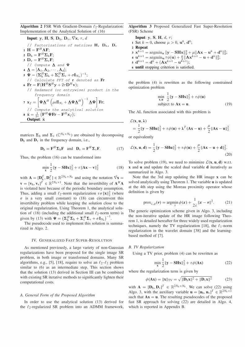
Algorithm 2 FSR With Gradient-Domain ℓ2-Regularization:Implementation of the Analytical Solution of (16)

matrices 6h and 6v (CNh×Nh ) are obtained by decomposingDh and Dv in the frequency domain, i.e.,

Dh = FH6hF and Dv = FH

6vF. (17)

Thus, the problem (16) can be transformed into

minx

1

2‖y − SHx‖22 + τ‖Ax − v‖22 (18)

with A = [DTh ,DT

v ] ∈ R2Nh ×Nh and using the notation ∇x =

v = [vh, vv]T ∈ R

2Nh×1. Note that the invertibility of AHA

is violated here because of the periodic boundary assumption.Thus, adding a small ℓ2-norm regularization τσ‖x‖22 (whereσ is a very small constant) to (18) can circumvent thisinvertibility problem while keeping the solution close to theoriginal regularization. Using Theorem 1, the analytical solu-tion of (18) (including the additional small ℓ2-norm term) isgiven by (13) with 9 =

(

6Hh 6h + 6

Hv 6v + σ INh

)−1.

The pseudocode used to implement this solution is summa-rized in Algo. 2.

IV. GENERALIZED FAST SUPER-RESOLUTION

As mentioned previously, a large variety of non-Gaussianregularizations have been proposed for the single image SRproblem, in both image or transformed domains. Many SRalgorithms, e.g., [5], [18], require to solve an ℓ2–ℓ2 problemsimilar to (6) as an intermediate step. This section showsthat the solution (13) derived in Section III can be combinedwith existing SR iterative methods to significantly lighten theircomputational costs.

A. General Form of the Proposed Algorithm

In order to use the analytical solution (13) derived forthe ℓ2-regularized SR problem into an ADMM framework,

Algorithm 3 Proposed Generalized Fast Super-Resolution(FSR) Scheme

the problem (4) is rewritten as the following constrainedoptimization problem

minx,u

1

2‖y − SHx‖22 + τφ(u)

subject to Ax = u. (19)

The AL function associated with this problem is

L(x,u,λ)

=1

2‖y − SHu‖22 + τφ(u) + λ

T (Ax − u) +µ

2‖Ax − u‖22

or equivalently

L(x,u,d) =1

2‖y − SHu‖22 + τφ(u) +

µ

2‖Ax − u + d‖22.

(20)

To solve problem (19), we need to minimize L(x,u,d) w.r.t.x and u and update the scaled dual variable d iteratively assummarized in Algo. 3.

Note that the 3rd step updating the HR image x can besolved analytically using Theorem 1. The variable u is updatedat the 4th step using the Moreau proximity operator whosedefinition is given by

proxλ,φ(ν) = argminx

φ(x) +1

2λ‖x − ν‖2. (21)

The generic optimization scheme given in Algo. 3, includingthe non-iterative update of the HR image following Theo-rem 1, is detailed hereafter for three widely used regularizationtechniques, namely the TV regularization [18], the ℓ1-normregularization in the wavelet domain [38] and the learning-based method of [7].

B. TV Regularization

Using a TV prior, problem (4) can be rewritten as

minx

1

2‖y − SHx‖22 + τφ(Ax) (22)

where the regularization term is given by

φ(Ax) = ‖x‖TV =√

‖Dhx‖2 + ‖Dvx‖2 (23)

with A = [Dh,Dv]T ∈ R2Nh×Nh . We can solve (22) using

Algo. 3, with the auxiliary variable u = [uh,uv]T ∈ R2Nh×1

such that Ax = u. The resulting pseudocodes of the proposedfast SR approach for solving (22) are detailed in Algo. 4,which is reported in Appendix B.

C. ℓ1-Norm Regularization in the Wavelet Domain

Assuming that x can be decomposed as a linear combinationof wavelets (e.g., as in [36]), the SR can be conductedin the wavelet domain. Denote as x = Wθ the waveletdecomposition of x, where θ ∈ RNh×1 is the vector containingthe wavelet coefficients and multiplying by the matrices WH

and W (∈ RNh×Nh ) represent the wavelet and inverse wavelettransforms (satisfying that WWH = WHW = INh ). Thesingle image SR with ℓ1-norm regularization in the waveletdomain can be formulated as follows

minx

1

2‖y − SHx‖22 + τ‖Ax‖1 (24)

where A = WH . By introducing the additional variableu = WHx, the problem (24) can be solved using Algo. 3. Thecorresponding pseudocodes of the resulting fast SR algorithmwith an ℓ1-norm regularization in the wavelet domain aredetailed in Algo. 5 in Appendix B.

D. Learning-Based ℓ2-Norm Regularization

The effectiveness of the learning-based regularization forimage reconstruction has been proved in several studies.In particular, Yang et al. [7] solved the single image SRproblem by jointly training two dictionaries for the LR andHR image patches and by applying sparse coding (SC).Interestingly, the HR image x0 obtained by SC was projectedonto the solution space satisfying (1), leading to the followingoptimization problem

x = argminx

1

2‖y − SHx‖22 + τ‖x − x0‖

22. (25)

This optimization problem was solved using a gradient descentapproach in [7]. However, it can benefit from the analyticalsolution provided by Theorem 1 that can be implemented usingAlgo. 1.

V. EXPERIMENTAL RESULTS

This section demonstrates the efficiency of the proposedfast SR strategy by testing it on various images with differentregularization terms. The performance of the single imageSR algorithms is evaluated in terms of reconstruction qualityand computational load. Given the ability of our algorithm tosolve the SR problem with less complexity than the existingmethods, one may expect a gain in computational time andconvergence properties. All the experiments were performedusing MATLAB 2013A on a computer with Windows 7,Intel(R) Core(TM) i7-4770 CPU @3.40GHz and 8 GB RAM.1

Color images were processed using the illuminate channelonly, as in [7]. Precisely, the RGB images were transformedinto YUV coordinates and the color channels (Cb,Cr) were up-sampled using bicubic interpolation. In the illuminate channel,the HR image was blurred and down-sampled in each spatialdirection with factors dr and dc. The resulting blurred and

1The MATLAB codes are available in the first author’s homepagehttp://zhao.perso.enseeiht.fr/.

decimated images were then contaminated by AWGN ofvariance σ 2

n with a blurred-signal-to-noise ratio defined by

BSNR = 10 log10

(

‖SHx − E(SHx)‖22Nσ 2

n

)

(26)

where N is the total number of pixels of the observed imageand E(·) is the arithmetic mean operator.

Unless explicitly specified, the blurring kernel is a2D-Gaussian filter of size 9 × 9 with variance σ 2

h = 3, thedecimation factors are dr = dc = 4 and the noise level isBSNR = 30dB.

The performances of the different SR algorithms are evalu-ated both visually and quantitatively in terms of the followingmetrics: root mean square error (RMSE), peak signal-to-noise ratio (PSNR), improved signal-to-noise ratio (ISNR)and mean structural similarity (MSSIM). The definitions ofthese metrics, widely used to evaluate image reconstructionmethods, are given below

RMSE =√

‖x − x‖2 (27)

PSNR = 20 log10max(x, x)

RMSE(28)

ISNR = 10 log10‖x − y‖2

‖x − x‖2(29)

MSSIM =1

M

M∑

j=1

SSIM(x j , x j ) (30)

where the vectors x, y, x are the ground truth (referenceimage/HR image), the bicubic interpolated image and therestored SR image respectively and max(x, x) defines thelargest value of x and x. Note that MSSIM is implementedblockwise, with M the number of local windows, x j and x j

are local regions extracted from x and x and SSIM is thestructural similarity measure of each window (defined in [49]).Note that it is nonsensical to compute the ISNR for bicubicinterpolation (always be 0) due to its definition.

A. Fast SR Using ℓ2-Regularizations

1) ℓ2 − ℓ2 Model in the Image Domain:

a) Gaussian blurring kernel: We first explore the singleimage SR problem with the “pepper” image and standardTikhonov/Gaussian regularization corresponding to the opti-mization problem formulated in (14). The size of the groundtruth HR image shown in Fig. 2(b) is 512×512. Fig. 2(c)–2(f)show the restored images with bicubic interpolation, the pro-posed analytical solution given in Algo. 1 and the splittingalgorithm ADMM of [18] adapted to a Gaussian prior. Theprior mean image x (approximated HR image) is the up-sampled version of the LR image by bicubic interpolation(Case 1) with the results in Fig. 2(e) and 2(d), whereas x is theground truth (Case 2) with the results in Fig. 2(g) and 2(f). Theregularization parameter was τ = 1 in Case 1 and τ = 0.1 inCase 2. The numerical results corresponding to this experimentare summarized in Table I. The visual impression and thenumerical results show that the reconstructed HR imagesobtained with our method are similar to those obtained withADMM. However, the proposed FSR method performs much

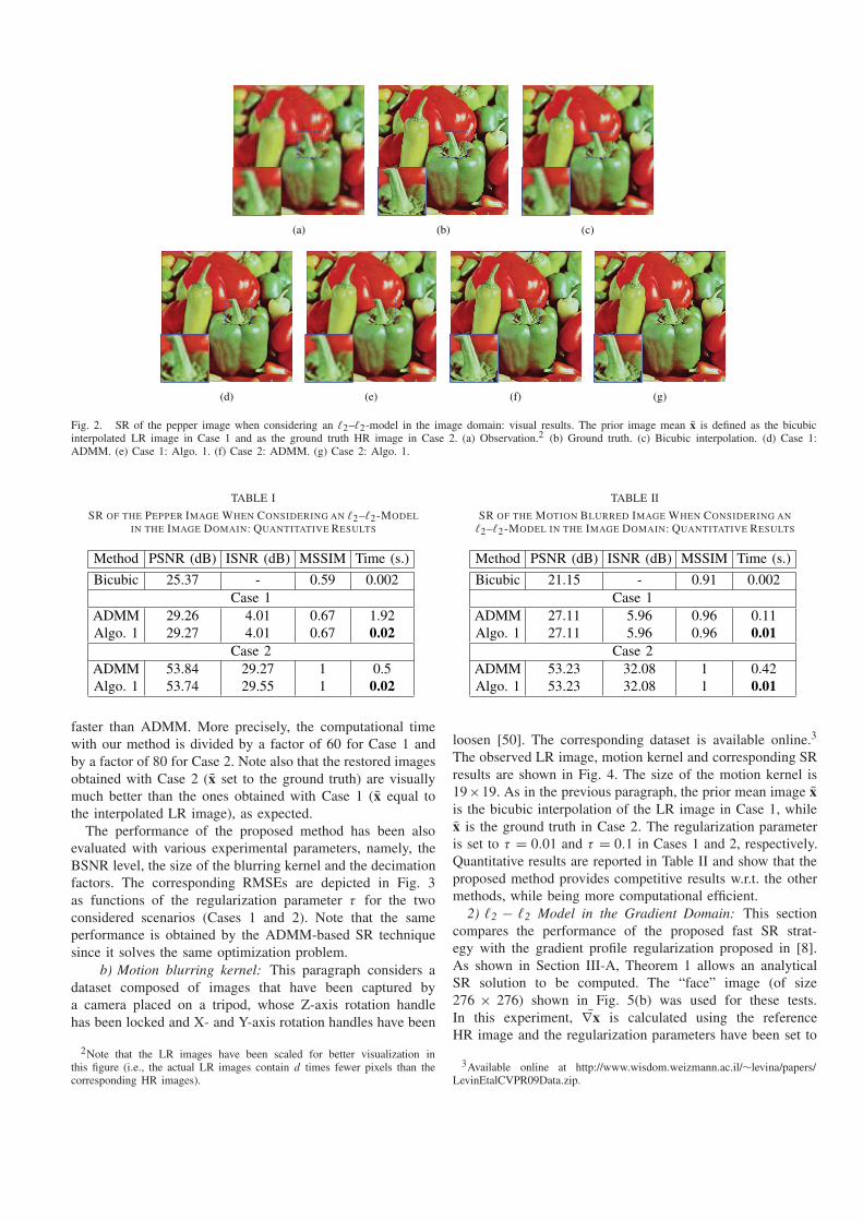
Fig. 2. SR of the pepper image when considering an ℓ2–ℓ2-model in the image domain: visual results. The prior image mean x is defined as the bicubicinterpolated LR image in Case 1 and as the ground truth HR image in Case 2. (a) Observation.2 (b) Ground truth. (c) Bicubic interpolation. (d) Case 1:ADMM. (e) Case 1: Algo. 1. (f) Case 2: ADMM. (g) Case 2: Algo. 1.

TABLE I

SR OF THE PEPPER IMAGE WHEN CONSIDERING AN ℓ2–ℓ2-MODEL

IN THE IMAGE DOMAIN: QUANTITATIVE RESULTS

faster than ADMM. More precisely, the computational timewith our method is divided by a factor of 60 for Case 1 andby a factor of 80 for Case 2. Note also that the restored imagesobtained with Case 2 (x set to the ground truth) are visuallymuch better than the ones obtained with Case 1 (x equal tothe interpolated LR image), as expected.

The performance of the proposed method has been alsoevaluated with various experimental parameters, namely, theBSNR level, the size of the blurring kernel and the decimationfactors. The corresponding RMSEs are depicted in Fig. 3as functions of the regularization parameter τ for the twoconsidered scenarios (Cases 1 and 2). Note that the sameperformance is obtained by the ADMM-based SR techniquesince it solves the same optimization problem.

b) Motion blurring kernel: This paragraph considers adataset composed of images that have been captured bya camera placed on a tripod, whose Z-axis rotation handlehas been locked and X- and Y-axis rotation handles have been

2Note that the LR images have been scaled for better visualization inthis figure (i.e., the actual LR images contain d times fewer pixels than thecorresponding HR images).

TABLE II

SR OF THE MOTION BLURRED IMAGE WHEN CONSIDERING AN

ℓ2–ℓ2 -MODEL IN THE IMAGE DOMAIN: QUANTITATIVE RESULTS

loosen [50]. The corresponding dataset is available online.3

The observed LR image, motion kernel and corresponding SRresults are shown in Fig. 4. The size of the motion kernel is19×19. As in the previous paragraph, the prior mean image x

is the bicubic interpolation of the LR image in Case 1, whilex is the ground truth in Case 2. The regularization parameteris set to τ = 0.01 and τ = 0.1 in Cases 1 and 2, respectively.Quantitative results are reported in Table II and show that theproposed method provides competitive results w.r.t. the othermethods, while being more computational efficient.

2) ℓ2 − ℓ2 Model in the Gradient Domain: This sectioncompares the performance of the proposed fast SR strat-egy with the gradient profile regularization proposed in [8].As shown in Section III-A, Theorem 1 allows an analyticalSR solution to be computed. The “face” image (of size276 × 276) shown in Fig. 5(b) was used for these tests.In this experiment, ∇x is calculated using the referenceHR image and the regularization parameters have been set to

3Available online at http://www.wisdom.weizmann.ac.il/∼levina/papers/LevinEtalCVPR09Data.zip.

Fig. 3. SR of the “pepper” image when considering the ℓ2–ℓ2 model in the image domain: RMSE as functions of the regularization parameter τ for variousnoise levels (1st column), blurring kernel sizes (2nd column) and decimation factors (3rd column). The results in the 1st column were obtained for dr = dc = 4and 9 × 9 kernel size; in the 2nd column, dr = dc = 4 and BSNR= 30 dB; in the 3rd column, the kernel size was 9 × 9 and BSNR= 30 dB.

Fig. 4. SR of the motion blurred image when considering an ℓ2–ℓ2-model in the image domain: visual results. The prior image mean x is defined asthe bicubic interpolated LR image in Case 1 and as the ground truth HR image in Case 2. (a) Observation. (b) Ground truth. (c) Bicubic interpolation.(d) Case 1: ADMM. (e) Case 1: Algo. 1. (f) Case 2: ADMM. (g) Case 2: Algo. 1.

τ = 10−3 and σ = 10−8. The proposed method is comparedwith the ADMM as well as the conjugate gradient (CG)method instead of the gradient descent (GD) method initiallyproposed in [17] (since CG has shown to be much moreefficient than GD in this experiment). The restored imagesusing bicubic interpolation, ADMM, the CG method and theproposed Algo. 2 are shown in Fig. 5(c)-5(e). The correspond-ing numerical results are reported in Table III. These resultsillustrate the superiority of the approach in terms of compu-tational time. This significant difference can be explained bythe non-iterative nature of the proposed method compared toCG and ADMM. Moreover, all the three methods converge to

the same global minimum as shown by the objective curves inFig. 6. The convergence of the objective curves is in agreementwith the visual and numerical results.

3) Learning-Based ℓ2-Norm Regularization: This sectionstudies the performance of the algorithm obtained whenthe analytical solution of Theorem 1 is embedded inthe learning-based method of [7]. The method investi-gated in [7] computed an initial estimation of the HRimage via SC and used a BP procedure to improve theSR performance. The BP operation was performed bya GD method in [7]. Here, this GD step has been replaced bythe analytical solution provided by Theorem 1 and Algo. 1.

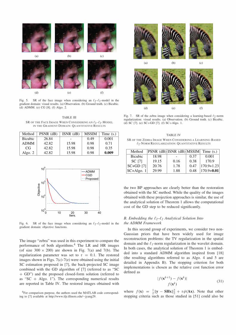
Fig. 5. SR of the face image when considering an ℓ2–ℓ2-model in thegradient domain: visual results. (a) Observation. (b) Ground truth. (c) Bicubic.(d) ADMM. (e) CG [8]. (f) Algo. 2.

TABLE III

SR OF THE FACE IMAGE WHEN CONSIDERING AN ℓ2–ℓ2-MODEL

IN THE GRADIENT DOMAIN: QUANTITATIVE RESULTS

Fig. 6. SR of the face image when considering an ℓ2–ℓ2-model in thegradient domain: objective functions.

The image “zebra” was used in this experiment to compare theperformance of both algorithms.4 The LR and HR images(of size 300 × 200) are shown in Fig. 7(a) and 7(b). Theregularization parameter was set to τ = 0.1. The restoredimages shown in Figs. 7(c)-7(e) were obtained using the initialSC estimation proposed in [7], the back-projected SC imagecombined with the GD algorithm of [7] (referred to as “SC+ GD”) and the proposed closed-form solution (referred toas “SC + Algo. 1”). The corresponding numerical resultsare reported in Table IV. The restored images obtained with

4For comparison purpose, the authors used the MATLAB code correspond-ing to [7] available at http://www.ifp.illinois.edu/∼jyang29.

Fig. 7. SR of the zebra image when considering a learning-based ℓ2-normregularization: visual results. (a) Observation. (b) Ground truth. (c) Bicubic.(d) SC [7]. (e) SC+GD [7]. (f) SC+Algo. 1.

TABLE IV

SR OF THE ZEBRA IMAGE WHEN CONSIDERING A LEARNING-BASED

ℓ2-NORM REGULARIZATION: QUANTITATIVE RESULTS

the two BP approaches are clearly better than the restorationobtained with the SC method. While the quality of the imagesobtained with these projection approaches is similar, the use ofthe analytical solution of Theorem 1 allows the computationalcost of the GD step to be reduced significantly.

B. Embedding the ℓ2–ℓ2 Analytical Solution Into

the ADMM Framework

In this second group of experiments, we consider two non-Gaussian priors that have been widely used for imagereconstruction problems: the TV regularization in the spatialdomain and the ℓ1-norm regularization in the wavelet domain.In both cases, the analytical solution of Theorem 1 is embed-ded into a standard ADMM algorithm inspired from [18](the resulting algorithms referred to as Algo. 4 and 5 aredetailed in Appendix B). The stopping criterion for bothimplementations is chosen as the relative cost function errordefined as

| f (xk+1) − f (xk)|

f (xk)(31)

where f (x) = 12‖y − SHx‖22 + τφ(Ax). Note that other

stopping criteria such as those studied in [51] could also be

Fig. 8. SR of the Monarch, Lena and Barbara images when considering a TV-regularization: visual results.

investigated. The 512 × 512 images “Lena”, “monarch” and“Barbara” were considered in these experiments. The observedLR images and the HR images (ground truth) are displayed inFig. 8 (first two columns).

1) TV-Regularization: The regularization parameter wasmanually fixed (by cross validation) to τ = 2 × 10−3 for theimage “Lena”, to τ = 1.8 × 10−3 for the image “monarch”and to τ = 2.5× 10−3 for the image “Barbara”. Fig. 8 showsthe SR results obtained using the bicubic interpolation (thirdcolumn), ADMM based algorithm of [18] (fourth column)and the proposed Algo. 4 (last column). As expected, theADMM reconstructions perform much better than a simpleinterpolation of the LR image that is not able to solve theupsampling and deblurring problem. The results obtained withthe proposed algorithm and with the method of [18] arevisually very similar. This visual inspection is confirmed bythe quantitative results provided in Table V. However, theproposed algorithm has the advantage of being much fasterthan the algorithm of [18] (with computational times reducedby a factor larger than 2). Moreover, Fig. 9 illustrates theconvergence of the two algorithms. The proposed single imageSR algorithm (Algo. 4) converges faster and with less fluctu-ations than the algorithm of [18]. This result can be explainedby the fact that the algorithme in [18] requires to handlemore variables in the ADMM scheme than the proposedalgorithm.

Fig. 9. SR of the Monarch, Lena and Barbara images when considering aTV-regularization: objective function (left) and ISNR (right) vs time.

2) ℓ1-Norm Regularization in the Wavelet Domain: Thissection evaluates the performance of Algo. 5, which is com-pared with a generalization of the method proposed in [18]

TABLE V

SR OF THE MONARCH, LENA AND BARBARA IMAGES WHEN CONSIDERING A TV-REGULARIZATION: QUANTITATIVE RESULTS

Fig. 10. SR of the Monarch, Lena and Barbara images when considering aℓ1-norm regularization in the wavelet domain: visual results.

to an ℓ1-norm regularization in the wavelet domain. Themotivations for working in the wavelet domain are essentiallyto take advantage of the sparsity of the wavelet coefficients.All experiments were conducted using the discrete Haarwavelet transform and the Rice wavelet toolbox [52]. For bothimplementations, the regularization parameter was adjusted bycross validation, leading to τ = 2×10−4 for the image “Lena”,τ = 1.8×10−4 for the image “Monarch” and τ = 2.5×10−4

for the image “Barbara”.Fig. 10 shows the SR reconstruction results with an

ℓ1-norm minimization in the wavelet domain. The HR images

Fig. 11. SR of the Monarch, Lena and Barbara images when considering anℓ1-norm regularization in the wavelet domain: objective function (left) andPSNR (right) vs time.

obtained with Algo. 5 and with the algorithm of [18] adaptedto the ℓ1-norm prior are visually similar and better than asimple interpolation. The numerical results shown in Table VIconfirm that the two algorithms provide similar reconstructionperformance. However, as in the previous case (TV regulariza-tion), the proposed algorithm is characterized by much smallercomputational times than the standard ADMM implementa-tion. The faster and smoother convergence obtained with theproposed method (Algo. 5) can be observed in Fig. 11. Notethat the fluctuations of the objective function and PSNR values(versus the number of iterations) obtained with the methodof [18] are due to the variable splitting, which requires morevariables and constraints to be handled than for the proposedmethod.

TABLE VI

SR OF THE MONARCH, LENA AND BARBARA IMAGES WHEN CONSIDERING A ℓ1-NORM REGULARIZATION

IN THE WAVELET DOMAIN: QUANTITATIVE RESULTS

VI. CONCLUSION AND PERSPECTIVES

This paper studied a new fast single image super-resolutionmethod based on the widely used image formation model.The proposed super-resolution approach computed the super-resolved image efficiently by exploiting intrinsic properties ofthe decimation and the blurring operators in the frequencydomain. A large variety of priors was shown to be able to behandled by the proposed super-resolution scheme. Specifically,when considering an ℓ2-regularization, the target image wascomputed analytically, getting rid of any iterative steps. Formore complex priors (i.e., non ℓ2-regularization), variablesplitting allowed this analytical solution to be embeddedinto the augmented Lagrangian framework, thus acceleratingvarious existing schemes for single image super-resolution.Results on several natural images confirmed the computationalefficiency of the proposed approach and showed its fast andsmooth convergence. As a perspective of this work, an interest-ing research track consists of extending the proposed methodto some online applications such as video super-resolution andmedical imaging, to evaluate its robustness to non-Gaussiannoise and to extend it to semi-blind or blind deconvolutionor multi-frame super-resolution. Considering a more practicalcase for super-resolving real images compressed by JPEG orJPEG-2000 algorithms would also deserve further exploration.

APPENDIX ADERIVATION OF THE ANALYTICAL SOLUTION (13)

The computational details for obtaining the result in(13) from (7) are summarized hereinafter. First, denotingr = HHSHy + 2τAHv, the solution (7) is

x = (HHSH + 2τAHA)−1r

= FH(

3HFSFH

3 + 2τFAHAFH)−1

Fr. (32)

Based on Lemma 1, 3HFSFH

3 is computed as

3HFSFH

3

=1

d3

H(

Jd ⊗ INl

)

3 (33)

=1

d3

H((

1d1Td

)

⊗(

INl INl

))

3 (34)

=1

d3

H(

1d ⊗ INl

)(

1Td ⊗ INl

)

3 (35)

Algorithm 4 FSR With TV Regularization

=1

d

3

H [INl , · · · , INl︸ ︷︷ ︸

d

]T

[INl , · · · , INl

︸ ︷︷ ︸

d

]3

(36)

=1

d3

H3. (37)

Note that (34) was obtained from (33) by replacing Jd by1d1

Td , where 1d ∈ Rd×1 is a vector of ones. Obtaining (35)

from (34) is straightforward using the following property ofthe Kronecker product ⊗

AB ⊗ CD = (A ⊗ C)(B ⊗ D).

Algorithm 5 FSR With ℓ1-Norm Regularization in the WaveletDomain

In (36), 3 ∈ RNh×Nh whereas[

INl , · · · , INl

]

∈ RNl ×Nh and[

INl , · · · , INl

]T∈ RNh ×Nl are block matrices whose blocks

are equal to the identity matrix INl . The matrix 3 ∈ RNl ×Nh

in (37) is given by

3 = [INl , · · · , INl ]3

= [INl , · · · , INl ]diag{31, · · · ,3d }

= [INl , · · · , INl ]

31 · · · 0...

. . ....

0 · · · 3d

(38)

= [31,32, · · · ,3d ]. (39)

As a consequence, (32) can be written as in (9), i.e.,

x = FH

(1

d3

H3 + 2τFAHAFH

)−1

Fr (40)

= FH

[

1

2τ9−

1

2τ93

H

(

dINl +1

2τ393

H

)−1

391

2τ

]

Fr

(41)

=1

2τFH

9Fr −1

2τFH

93H

(

2τdINl + 393H

)−139Fr

(42)

where 9 = F(

AHA)−1

FH . The Lemma 2 is adopted from(40) to (41) with A1 = 2τFAHAFH , A2 = 3

H , A3 = 1dI

and A4 = 3. Note that the matrices A1 and A3 are alwaysinvertible, implying that the Woodbury formula can be applied.

APPENDIX BPSEUDO CODES OF THE PROPOSED FAST ADMMSUPER-RESOLUTION METHODS FOR TV AND

ℓ1-NORM REGULARIZATIONS

See Algorithms 4 and 5.

REFERENCES

[1] S. C. Park, M. K. Park, and M. G. Kang, “Super-resolution imagereconstruction: A technical overview,” IEEE Signal Process. Mag.,vol. 20, no. 3, pp. 21–36, May 2003.

[2] G. Martín and J. M. Bioucas-Dias, “Hyperspectral compressiveacquisition in the spatial domain via blind factorization,” in Proc.IEEE Workshop Hyperspectral Image Signal Process., Evol. Remote

Sens. (WHISPERS), Tokyo, Japan, Jun. 2015, pp. 1–4.[3] J. Yang and T. Huang, “Image super-resolution: Historical overview and

future challenges,” in Super-Resolution Imaging. Boca Raton, FL, USA:CRC Press, 2010, pp. 20–34.

[4] T. Akgun, Y. Altunbasak, and R. M. Mersereau, “Super-resolutionreconstruction of hyperspectral images,” IEEE Trans. Image Process.,vol. 14, no. 11, pp. 1860–1875, Nov. 2005.

[5] I. Yanovsky, B. H. Lambrigtsen, A. B. Tanner, and L. A. Vese, “Efficientdeconvolution and super-resolution methods in microwave imagery,”IEEE J. Sel. Topics Appl. Earth Observ. Remote Sens., vol. 8, no. 9,pp. 4273–4283, Sep. 2015.

[6] R. Morin, A. Basarab, and D. Kouamé, “Alternating direction methodof multipliers framework for super-resolution in ultrasound imaging,”in Proc. 9th IEEE Int. Symp. Biomed. Imag. (ISBI), Barcelona, Spain,May 2012, pp. 1595–1598.

[7] J. Yang, J. Wright, T. S. Huang, and Y. Ma, “Image super-resolutionvia sparse representation,” IEEE Trans. Image Process., vol. 19, no. 11,pp. 2861–2873, Nov. 2010.

[8] J. Sun, J. Sun, Z. Xu, and H.-Y. Shum, “Image super-resolution usinggradient profile prior,” in Proc. IEEE Conf. Comput. Vis. PatternRecognit. (CVPR), Anchorage, AK, USA, Jun. 2008, pp. 1–8.

[9] Y.-W. Tai, S. Liu, M. S. Brown, and S. Lin, “Super resolution using edgeprior and single image detail synthesis,” in Proc. IEEE Conf. Comput.Vis. Pattern Recognit. (CVPR), San Francisco, CA, USA, Jun. 2010,pp. 2400–2407.

[10] P. Thévenaz, T. Blu, and M. Unser, “Image interpolation and resam-pling,” in Handbook of Medical Imaging, I. N. Bankman, Ed. Orlando,FL, USA: Academic, 2000, pp. 393–420.

[11] X. Zhang and X. Wu, “Image interpolation by adaptive 2-D autore-gressive modeling and soft-decision estimation,” IEEE Trans. Image

Process., vol. 17, no. 6, pp. 887–896, Jun. 2008.[12] S. Mallat and Y. Guoshen, “Super-resolution with sparse mixing esti-

mators,” IEEE Trans. Image Process., vol. 19, no. 11, pp. 2889–2900,Nov. 2010.

[13] W. T. Freeman, E. C. Pasztor, and O. T. Carmichael, “Learning low-levelvision,” Int. J. Comput. Vis., vol. 40, no. 1, pp. 25–47, Oct. 2000.

[14] D. Glasner, S. Bagon, and M. Irani, “Super-resolution from a singleimage,” in Proc. IEEE Int. Conf. Comput. Vis. (ICCV), Kyoto, Japan,Sep./Oct. 2009, pp. 349–356.

[15] J.-B. Huang, A. Singh, and N. Ahuja, “Single image super-resolutionfrom transformed self-exemplars,” in Proc. IEEE Conf. Comput.

Vis. Pattern Recognit. (CVPR), Boston, MA, USA, Jun. 2015,pp. 5197–5206.

[16] R. Zeyde, M. Elad, and M. Protter, “On single image scale-up usingsparse-representations,” in Curves and Surfaces (Lecture Notes in Com-puter Science), J.-D. Boissonnat et al., Eds. Heidelberg, Germany:Springer, 2012, pp. 711–730.

[17] J. Sun, J. Sun, Z. Xu, and H.-Y. Shum, “Gradient profile prior and itsapplications in image super-resolution and enhancement,” IEEE Trans.Image Process., vol. 20, no. 6, pp. 1529–1542, Jun. 2011.

[18] M. K. Ng, P. Weiss, and X. Yuan, “Solving constrained total-variationimage restoration and reconstruction problems via alternating directionmethods,” SIAM J. Sci. Comput., vol. 32, no. 5, pp. 2710–2736,2010.

[19] A. Beck and M. Teboulle, “A fast iterative shrinkage-thresholdingalgorithm for linear inverse problems,” SIAM J. Imag. Sci., vol. 2, no. 1,pp. 183–202, Mar. 2009.

[20] A. Marquina and S. J. Osher, “Image super-resolution byTV-regularization and Bregman iteration,” J. Sci. Comput., vol. 37,no. 3, pp. 367–382, Dec. 2008.

[21] W. Yin, S. Osher, D. Goldfarb, and J. Darbon, “Bregman iterative algo-rithms for ℓ1-minimization with applications to compressed sensing,”SIAM J. Imag. Sci., vol. 1, no. 1, pp. 143–168, 2008.

[22] M. D. Robinson, C. A. Toth, J. Y. Lo, and S. Farsiu, “Efficient Fourier-wavelet super-resolution,” IEEE Trans. Image Process., vol. 19, no. 10,pp. 2669–2681, Oct. 2010.

[23] F. Šroubek, J. Kamenický, and P. Milanfar, “Superfast superresolution,”in Proc. IEEE Int. Conf. Image Process. (ICIP), Brussels, Belgium,Sep. 2011, pp. 1153–1156.

[24] M. Ebrahimi and E. R. Vrscay, “Regularization schemes involving self-similarity in imaging inverse problems,” in Proc. 4th AIP Int. Conf., 1st

Congr. IPIA, 2008, pp. 1–12.[25] K. Zhang, X. Gao, D. Tao, and X. Li, “Single image super-resolution

with non-local means and steering kernel regression,” IEEE Trans. Image

Process., vol. 21, no. 11, pp. 4544–4556, Nov. 2012.[26] M. Elad and A. Feuer, “Restoration of a single superresolution image

from several blurred, noisy, and undersampled measured images,” IEEE

Trans. Image Process., vol. 6, no. 12, pp. 1646–1658, Dec. 1997.[27] S. Farsiu, D. Robinson, M. Elad, and P. Milanfar, “Advances and

challenges in super-resolution,” Int. J. Imag. Syst. Technol., vol. 14, no. 2,pp. 47–57, 2004.

[28] Z. Lin and H.-Y. Shum, “Fundamental limits of reconstruction-basedsuperresolution algorithms under local translation,” IEEE Trans. PatternAnal. Mach. Intell., vol. 26, no. 1, pp. 83–97, Jan. 2004.

[29] J. K. H. Ng, “Restoration of medical pulse-echo ultrasound images,”Ph.D. dissertation, Dept. Eng., Trinity College, Univ. Cambridge,Cambridge, U.K., 2006.

[30] N. Zhao, A. Basarab, and D. Kouamé, and J.-Y. Tourneret. (2015).“Joint segmentation and deconvolution of ultrasound images using ahierarchical Bayesian model based on generalized Gaussian priors.”[Online]. Available: http://arxiv.org/abs/1412.2813

[31] C. P. Robert, The Bayesian Choice: From Decision-Theoretic Founda-

tions to Computational Implementation (Springer Texts in Statistics),2nd ed. New York, NY, USA: Springer-Verlag, 2007.

[32] A. Gelman, J. B. Carlin, H. S. Stern, D. B. Dunson, A. Vehtari, andD. B. Rubin, Bayesian Data Analysis, 3rd ed. Boca Raton, FL, USA:CRC Press, 2013.

[33] N. Nguyen, P. Milanfar, and G. Golub, “A computationally efficientsuperresolution image reconstruction algorithm,” IEEE Trans. Image

Process., vol. 10, no. 4, pp. 573–583, Apr. 2001.[34] Q. Wei, J. Bioucas-Dias, N. Dobigeon, and J.-Y. Tourneret, “Hyperspec-

tral and multispectral image fusion based on a sparse representation,”IEEE Trans. Geosci. Remote Sens., vol. 53, no. 7, pp. 3658–3668,Jul. 2015.

[35] H. A. Aly and E. Dubois, “Image up-sampling using total-variationregularization with a new observation model,” IEEE Trans. Image

Process., vol. 14, no. 10, pp. 1647–1659, Oct. 2005.[36] J. M. Bioucas-Dias, “Bayesian wavelet-based image deconvolution:

A GEM algorithm exploiting a class of heavy-tailed priors,” IEEE Trans.

Image Process., vol. 15, no. 4, pp. 937–951, Apr. 2006.[37] J. Ng, R. Prager, N. Kingsbury, G. Treece, and A. Gee, “Wavelet

restoration of medical pulse-echo ultrasound images in an EM frame-work,” IEEE Trans. Ultrason., Ferroelectr., Freq. Control, vol. 54, no. 3,pp. 550–568, Mar. 2007.

[38] C. V. Jiji, M. V. Joshi, and S. Chaudhuri, “Single-frame imagesuper-resolution using learned wavelet coefficients,” Int. J. Imag. Syst.

Technol., vol. 14, no. 3, pp. 105–112, 2004.[39] M. A. T. Figueiredo and R. D. Nowak, “An EM algorithm for wavelet-

based image restoration,” IEEE Trans. Image Process., vol. 12, no. 8,pp. 906–916, Aug. 2003.

[40] R. Fattal, “Edge-avoiding wavelets and their applications,” ACM Trans.

Graph., vol. 28, no. 3, pp. 1–10, Aug. 2009.[41] S. Roth and M. J. Black, “Fields of experts: A framework for

learning image priors,” in Proc. IEEE Conf. Comput. Vis. Pattern

Recognit. (CVPR), Jun. 2005, pp. 860–867.[42] D. Zoran and Y. Weiss, “From learning models of natural image patches

to whole image restoration,” in Proc. IEEE Int. Conf. Comp. Vis. (ICCV),Barcelona, Spain, Nov. 2011, pp. 479–486.

[43] H. W. Engl, M. Hanke, and A. Neubauer, Regularization inverseproblems. Springer Science & Business Media, 1996, vol. 375.

[44] O. Féron, F. Orieux, and J.-F. Giovannelli. (2015). “Gradient scanGibbs sampler: An efficient algorithm for high-dimensional Gaussiandistributions.” [Online]. Available: http://arxiv.org/abs/1509.03495

[45] F. Orieux, O. Féron, and J. F. Giovannelli, “Sampling high-dimensionalGaussian distributions for general linear inverse problems,” IEEE Signal

Process. Lett., vol. 19, no. 5, pp. 251–254, May 2012.[46] C. Gilavert, S. Moussaoui, and J. Idier, “Efficient Gaussian sampling for

solving large-scale inverse problems using MCMC,” IEEE Trans. Signal

Process., vol. 63, no. 1, pp. 70–80, Jan. 2015.[47] W. W. Hager, “Updating the inverse of a matrix,” SIAM Rev., vol. 31,

no. 2, pp. 221–239, 1989.[48] Q. Wei, N. Dobigeon, and J.-Y. Tourneret, “Bayesian fusion of multi-

band images,” IEEE J. Sel. Topics Signal Process., vol. 9, no. 6, p. 1127,Sep. 2015.

[49] Z. Wang, A. C. Bovik, H. R. Sheikh, and E. P. Simoncelli, “Imagequality assessment: From error visibility to structural similarity,” IEEE

Trans. Image Process., vol. 13, no. 4, pp. 600–612, Apr. 2004.[50] A. Levin, Y. Weiss, F. Durand, and W. T. Freeman, “Understanding

and evaluating blind deconvolution algorithms,” in Proc. IEEE Conf.

Comput. Vis. Patt. Recognit. (CVPR), Miami, FL, USA, Jun. 2009,pp. 1964–1971.

[51] S. Boyd, N. Parikh, E. Chu, B. Peleato, and J. Eckstein, “Distributedoptimization and statistical learning via the alternating direction methodof multipliers,” Found. Trends Mach. Learn., vol. 3, no. 1, pp. 1–122,Jan. 2011.

[52] R. Baraniuk et al. Rice Wavelet Toolbox, accessed on Dec. 1, 2002.[Online]. Available: http://dsp.rice.edu/software/rice-wavelet-toolbox

Ningning Zhao received the B.Sc. degree fromJilin University, China, in 2011, the master’sdegree from the Electrical Engineering Department,Beihang University, Beijing, China, in 2012, andthe M.Sc. degree from the University of Toulouse,France, in 2013, where she is currently pursuing thePh.D. degree. She is currently with the Signal andCommunication Group and also Image Comprehen-sion and Processing Group with IRIT Laboratory.Her research interests include medical imaging andinverse problems of image processing, particularly

image deconvolution and segmentation. He has served as a Reviewer of theIEEE TRANSACTIONS ON IMAGE PROCESS.

Qi Wei (S’13) was born in Shanxi, China, in 1989.He received the Ph.D. degree in signal and imageprocessing from the National Polytechnic Institute ofToulouse, University of Toulouse, France, in 2015,and the bachelor’s degree in electrical engineeringfrom Beihang University, Beijing, China, in 2010.His Ph.D. thesis, Bayesian Fusion of Multi-bandImages: A Powerful Tool for Super-Resolution, wasrated as one of the best theses (received Prix LèopoldEscande) with University of Toulouse, in 2015.In 2012, he was an Visiting Student with the Signal

Processing and Communications Group, Department of Signal Theory andCommunications, Universitat Politècnica de Catalunya. Since 2015, he hasbeen a Research Associate with the Signal Processing Laboratory, Departmentof Engineering, University of Cambridge. His research has been focusedon inverse problems in image processing, Bayesian statistical inferenceand parameter estimation, and optimization algorithms in large scale dataprocessing. He has served as a Reviewer of the IEEE TRANSACTION ON

IMAGE PROCESS, the IEEE JOURNAL OF SELECTED TOPICS IN SIGNAL

PROCESSING, the IEEE TRANSACTIONS ON GEOSCIENCE AND REMOTE

SENSING, and several conferences.

Adrian Basarab received the M.S. and Ph.D.degrees in signal and image processing from theNational Institute for Applied Sciences of Lyon,France, in 2005 and 2008, respectively. Since 2009,he has been an Assistant Professor with the Univer-sity Paul Sabatier Toulouse 3 and a member of IRITlaboratory. His research interests include medicalimaging, and more particularly motion estimation,inverse problems, and ultrasound image formation.He is an Associate Editor of the Digital Signal

Processing.

Nicolas Dobigeon (S’05–M’08–SM’13) was bornin Angoulême, France, in 1981. He receivedthe Engineering degree in electrical engineeringfrom ENSEEIHT, Toulouse, France, in 2004, andthe M.Sc. degree in signal processing from INPToulouse, in 2004, the Ph.D. degree and the Habili-tation à Diriger des Recherches in signal processingfrom INP Toulouse, in 2007 and 2012, respectively.From 2007 to 2008, he was a Post-Doctoral ResearchAssociate with the Department of ElectricalEngineering and Computer Science, University of

Michigan, Ann Arbor. Since 2008, he has been with INP-ENSEEIHTToulouse, University of Toulouse, where he is currently an Associate Profes-sor. He conducts his research within the Signal and Communications Group,IRIT Laboratory, and he is also an Affiliated Faculty Member of the TeSALaboratory. His recent research activities have been focused on statisticalsignal and image processing, with a particular interest in Bayesian inverseproblems with applications to remote sensing and biomedical imaging.

Denis Kouamé (M’97) received the Ph.D. andHabilitation à Diriger des Recherches degrees in sig-nal processing and medical ultrasound imaging fromthe University of Tours, Tours, France, in 1996 and2004, respectively. He is currently a Professor withthe Paul Sabatier University of Toulouse, Toulouse,France, and a member of the IRIT Laboratory. From1998 to 2008, he was an Assistant and then anAssociate Professor with the University of Tours.From 1996 to 1998, he was a Senior Engineer withthe GIP Tours, Tours, France. He was the Head of

the Signal and Image Processing Group, and then the Head of UltrasoundImaging Group, Ultrasound and Signal Laboratory, University of Tours,from 2000 to 2006 and from 2006 to 2008. He currently leads the ImageComprehension and Processing Group, IRIT. His research interests are focusedon signal and image processing with applications to medical imaging andparticularly ultrasound imaging, including high resolution imaging, imageresolution enhancement, doppler signal processing, detection and estimationwith application to cerebral emboli detection, multidimensional parametricmodeling, spectral analysis, and inverse problems related to compressedsensing and restoration. He has been involved in the organization of severalconferences. He has also led a number of invited conferences, specialsessions and tutorials in this area at several IEEE conferences and workshops.He has been serving as an Associate Editor of the IEEE TRANSACTIONS ON

ULTRASONICS, FERROELECTRICS, AND FREQUENCY CONTROL.

Jean-Yves Tourneret (SM’08) received theIngénieur degree in electrical engineering from theUniversity of Toulouse, Toulouse, in 1989, andthe Ph.D. degree from the INP Toulouse, in 1992.He is currently a Professor with the University ofToulouse and a member of the IRIT Laboratory. Hisresearch activities are centered around statisticalsignal and image processing with a particularinterest to Bayesian and Markov chain Monte Carlomethods. He has been involved in the organizationof several conferences, including the European

Conference on Signal Processing in 2002 (Program Chair), the internationalconference ICASSP’6 (plenaries), the Statistical Signal Processing Workshop2012 (International Liaisons), the International Workshop on ComputationalAdvances in Multi-Sensor Adaptive Processing in 2013 (local arrangements),the Statistical Signal Processing Workshop in 2014 (special sessions), theWorkshop on Machine Learning for Signal Processing in 2014 (specialsessions). He has been the General Chair of the CIMI Workshop onOptimization and Statistics in Image processing hold in Toulouse, in 2013(with F. Malgouyres and D. Kouamé) and of the International Workshopon Computational Advances in Multi-Sensor Adaptive Processing in 2015(with P. Djuric). He has been a member of different technical committeesincluding the Signal Processing Theory and Methods Committee of theIEEE Signal Processing Society (2001–2007, 2010–2015). He has beenserving as an Associate Editor of the IEEE TRANSACTIONS ON SIGNAL

PROCESSING (2008–2011, 2015-present) and for the EURASIP journal on

Signal Processing (2013-present).