Online parameter estimation applied to mixed
17
Transcript of Online parameter estimation applied to mixed

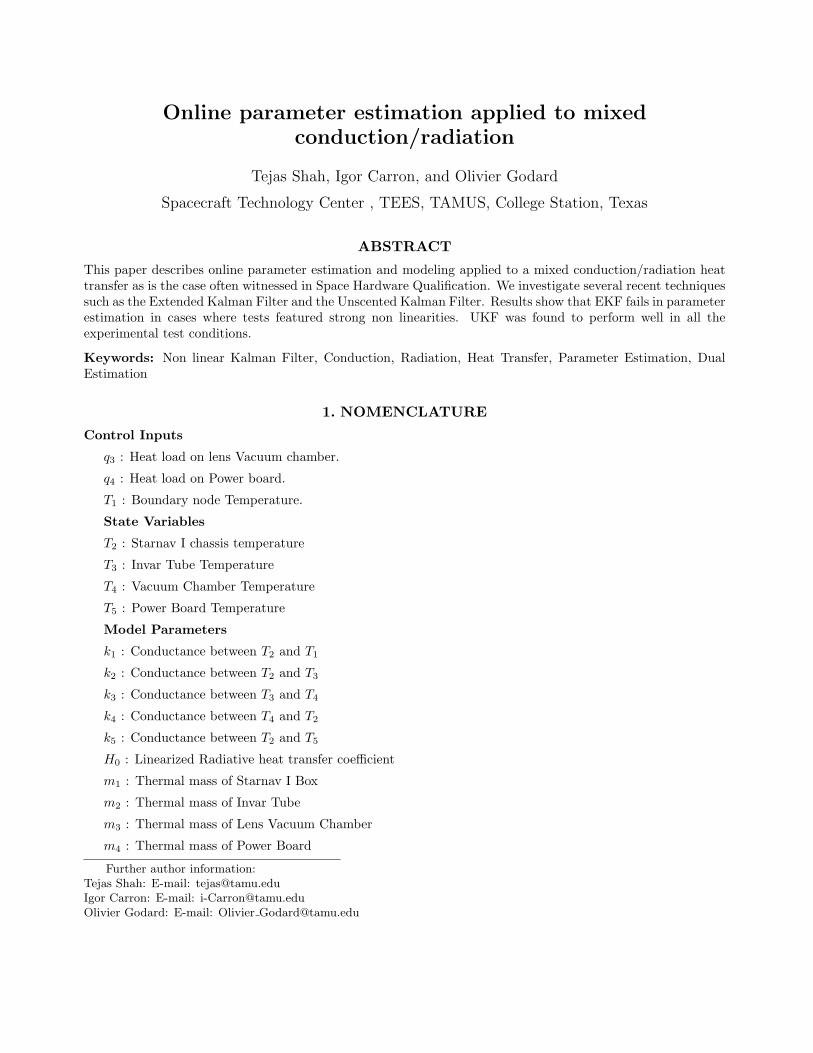
Online parameter estimation applied to mixedconduction/radiation
Tejas Shah, Igor Carron, and Olivier Godard
Spacecraft Technology Center , TEES, TAMUS, College Station, Texas
ABSTRACT
This paper describes online parameter estimation and modeling applied to a mixed conduction/radiation heattransfer as is the case often witnessed in Space Hardware Qualification. We investigate several recent techniquessuch as the Extended Kalman Filter and the Unscented Kalman Filter. Results show that EKF fails in parameterestimation in cases where tests featured strong non linearities. UKF was found to perform well in all theexperimental test conditions.
Keywords: Non linear Kalman Filter, Conduction, Radiation, Heat Transfer, Parameter Estimation, DualEstimation
1. NOMENCLATURE
Control Inputs
q3 : Heat load on lens Vacuum chamber.
q4 : Heat load on Power board.
T1 : Boundary node Temperature.
State Variables
T2 : Starnav I chassis temperature
T3 : Invar Tube Temperature
T4 : Vacuum Chamber Temperature
T5 : Power Board Temperature
Model Parameters
k1 : Conductance between T2 and T1
k2 : Conductance between T2 and T3
k3 : Conductance between T3 and T4
k4 : Conductance between T4 and T2
k5 : Conductance between T2 and T5
H0 : Linearized Radiative heat transfer coefficient
m1 : Thermal mass of Starnav I Box
m2 : Thermal mass of Invar Tube
m3 : Thermal mass of Lens Vacuum Chamber
m4 : Thermal mass of Power Board
Further author information:Tejas Shah: E-mail: [email protected] Carron: E-mail: [email protected] Godard: E-mail: Olivier [email protected]

2. INTRODUCTION
The objective often is to obtain model parameters from experimental data. We present online state and pa-rameter estimation applied to temperature data from different environmental test on a payload (StarNav I).A five node simplified model is built to understand the dynamics of the system. A state space model is thenbuilt from the nodal equations of this model. The parameters (like conductance or thermal masses) are firstestimated from the observations from four thermal tests performed on the ground, using initial guesses obtainedof the CAD model built in Thermal Desktop c©9 . Using this data, a new estimation can then be performed onthe data obtained during flight for parameters which could not be obtained on the ground (environmental heatloads).
Two methods are used to estimate the model parameters, the Extended Kalman Filter(EKF) and UnscentedKalman Filter(UKF). Both of these methods are described briefly below.
3. KALMAN FILTER
The Kalman filter provides a recursive solution to the linear optimal filtering problem. The solution is recursivein that each updated estimate of the state is computed from the previous estimate and the new input data, soonly the previous estimate requires storage. The Kalman filter is computationally more efficient than computingthe estimate directly form the entire past observed data at each step of the filtering process. Most of the followinginformation on Kalman filtering is obtained from ”Kalman Filtering and Neural Networks” by S. Haykin.1
The Kalman filter is based on the following two equations:
1. Process equation:xk+1 = Fk+1,kxk + wk (1)
where Fk+1,k is the transition matrix taking the state xk from time k to time k+1. The process noise wk isassumed to be white and Gaussian, with zero mean and with the covariance matrix defined by
E[wnwTn ] =
{Qk for n = k0 for n 6= k
}(2)
where the superscript T denotes transposition. The dimension of the state space is denoted by M.
2. Measurement equation:yk = Hkxk + vk (3)
where yk is the observation vector at time k and Hk is the measurement matrix. The measurement noise vk
is assumed to be additive, white, and Gaussian, with zero mean and with the covariance matrix defined by
E[vnvTn ] =
{Rk for n = k0 for n 6= k
}(4)
In equations (1) and (3) , the measurement noise vk is uncorrelated with the process noise wk. The dimensionof the measurement space is denoted by N. The Kalman filtering process is the solving of the process and mea-surement equations for the unknown state in an optimum manner. It uses the entire observed data y1, y2, · · · yk
to find for each k ≥ 1 the minimum mean square error estimate of the state xi.
4. EXTENDED KALMAN FILTER
The Kalman filter only addresses the estimation of a state vector in a linear model. If the model is nonlinear, theKalman filter can be extended through a linearization procedure yielding the Extended Kalman Filter (EKF).This extension is feasible because the Kalman filter is described in terms of difference equations in the case ofdiscrete-time systems. Consider a nonlinear dynamical system described by the following state-space model:
xk+1 = f(k, xk) + wk (5)

yk = h(k, xk) + vk (6)
where wk and vk are independent zero-mean white Gaussian noise processes with covariance matrices Rk and Qk,respectively. The functional f(k, xk) denotes a nonlinear transition matrix function that is possibly time-variant.The functional h(k, xk) denotes a nonlinear measurement matrix that also may be time-variant.
The idea of the extended Kalman filter is to linearize the state space model at each time instant aroundthe most recent state estimate, which is taken to be either the current estimate xk or the prior estimate x−k ,depending on which particular functional is being considered. After linearizing the model, the standard Kalmanfilter equations can be applied. This is done in two stages:
Stage 1:
Fk+1,k =∂f(k, x)
∂x x=xk
(7)
Hk =∂h(k, xk)
∂x x=x−k
(8)
The ij-th entry of Fk+1,k is equal to the partial derivative of the i-th component of F (k, x) with respect tothe j-th component of x. The ij-th component of Hk is equal to the partial derivative of the i-th component ofH(k, x) with respect to the j-th component of x.
Stage 2:
Once the matrices Fk+1,k and Hk are evaluated, they are used in the first-order Taylor approximation of thenonlinear functions F(k, xk) and H(k, xk) around xk and x−k .
F (k, xk) ≈ F (x, xk) + Fk+1,k(x, xk) (9)
H(k, xk) ≈ H(x, xk) + Hk+1,k(x, x−k ) (10)
hence the non linear state equations are given as
xk+1 ≈ Fk+1,kxk + wk + dk (11)
yk ≈ Hkxk + vk (12)
whereyk = yk − h(x, x−k )−Hkx−k (13)
dk = f(x, xk)− Fk+1,kxk (14)
5. UNSCENTED KALMAN FILTER
Because EKF relies on a linear approximation of the non linear functions F and H, it has shown to fail ininstances of strong non linearities. The Unscented Kalman filter addresses this approximation issue with UKF.The distribution of the state variable is represented by a Gaussian random variable, and is specified using aminimal set of carefully chosen sample points. The sample points capture the mean and covariance of theGaussian random variable1234 .
Unscented Transformation
The Unscented Transformation is a method for calculating the statistics of a random variable which undergoesa nonlinear transformation. For more information refer.1
Unscented Kalman Filter
The Unscented Kalman filter is an extension of the Unscented Transformation. No explicit calculations orJacobians or Hessians are necessary to implement this algorithm.
6. APPLICATION TO STARNAV IStarNav I is an advanced star tracker designed and built by the Spacecraft Technology Center and the AerospaceEngineering Department at Texas A&M University, It flew during the STS-107 mission aboard the Space ShuttleColumbia. Its objective was to validate the Lost in space algorithm (LISA) developed by Dr. Junkins fordetermining precise spacecraft attitude without prior knowledge of position.6 In order to successfully passsafety reviews, the StarNav I payload went through different thermal vacuum tests. The goal of this paper isto show how the thermal model of the payload was estimated through the course of the various thermal tests.
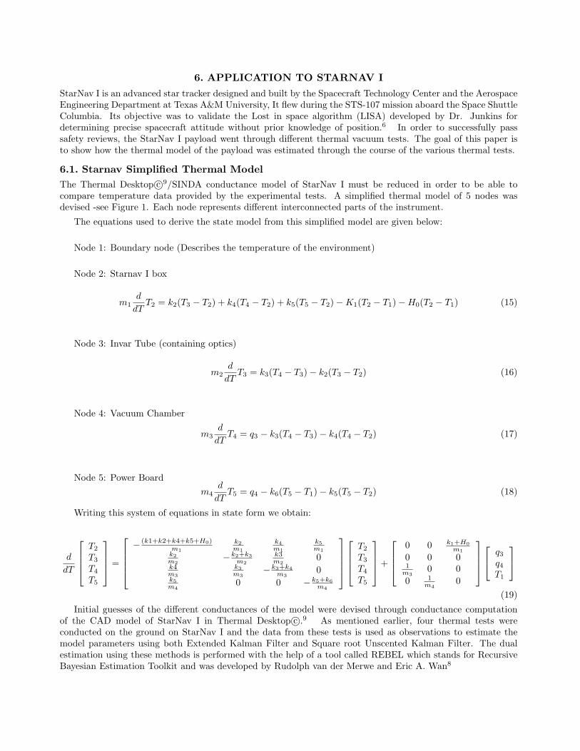
6.1. Starnav Simplified Thermal ModelThe Thermal Desktop c©9/SINDA conductance model of StarNav I must be reduced in order to be able tocompare temperature data provided by the experimental tests. A simplified thermal model of 5 nodes wasdevised -see Figure 1. Each node represents different interconnected parts of the instrument.
The equations used to derive the state model from this simplified model are given below:
Node 1: Boundary node (Describes the temperature of the environment)
Node 2: Starnav I box
m1d
dTT2 = k2(T3 − T2) + k4(T4 − T2) + k5(T5 − T2)−K1(T2 − T1)−H0(T2 − T1) (15)
Node 3: Invar Tube (containing optics)
m2d
dTT3 = k3(T4 − T3)− k2(T3 − T2) (16)
Node 4: Vacuum Chamber
m3d
dTT4 = q3 − k3(T4 − T3)− k4(T4 − T2) (17)
Node 5: Power Boardm4
d
dTT5 = q4 − k6(T5 − T1)− k5(T5 − T2) (18)
Writing this system of equations in state form we obtain:
d
dT
T2
T3
T4
T5
=
− (k1+k2+k4+k5+H0)
m1
k2m1
k4m1
k5m1
k2m2
−k2+k3m2
k3m2
0k4m3
k3m3
−k3+k4m3
0k5m4
0 0 −k5+k6m4
T2
T3
T4
T5
+
0 0 k1+H0
m1
0 0 01
m30 0
0 1m4
0
q3
q4
T1
(19)
Initial guesses of the different conductances of the model were devised through conductance computationof the CAD model of StarNav I in Thermal Desktop c©.9 As mentioned earlier, four thermal tests wereconducted on the ground on StarNav I and the data from these tests is used as observations to estimate themodel parameters using both Extended Kalman Filter and Square root Unscented Kalman Filter. The dualestimation using these methods is performed with the help of a tool called REBEL which stands for RecursiveBayesian Estimation Toolkit and was developed by Rudolph van der Merwe and Eric A. Wan8

7. GROUND TEST DESCRIPTION AND RESULTSThe results obtained from the test data parameter estimation process are described below.
For Figures 3 to 12, it can can be observed that the estimated states (temperatures of the invar tube-T3, thevacuum chamber-T4, and the power board-T5) are correlating with the observation (top section of the figure)and that the estimated parameters (bottom section) are converging toward a asymptotic value quickly. Theinitial discrepancy between state and observation is due to the parameter estimation.
Test-A1 This test was conducted in thermal vacuum at 290K. The results from the test and parameterestimation subroutines are presented in Figures 3 and 4. Figure 3 presents estimation using the Square RootUnscented Kalman Filter. The bottom part presents the estimation of 1
m4and k4
m3, where m4 is the thermal
mass of the power board, m3 the thermal mass of vacuum chamber, and k4 the conductance between T4 andT2. Figure 4 presents the results obtained using the Extended Kalman Filter. These results are essentially thesame as the ones presented in Figure 3 using UKF.
Test-A2 This test was conducted in thermal vacuum at 290K. The results from the test and parameterestimation subroutines are presented in Figures 5 and 6. Figure 5 presents estimation using the Square RootUnscented Kalman Filter. The bottom part presents the estimation of 1
m3and k5
m4, where m3 is the thermal
mass of the vacuum chamber, m4 the thermal mass of the power board, and k5 the conductance between T2and T5. Figure 6 presents the results obtained using the Extended Kalman Filter. These results are essentiallythe same as the ones presented in Figure 5 using UKF.
Test-A3 This test was conducted in thermal vacuum at 290K. The results from the test and parameterestimation subroutines are presented in Figures 7 and 8. Figure 7 presents estimation using the Square RootUnscented Kalman Filter. The bottom part presents the estimation of k2
m2and k3
m3, where m2 is the thermal
mass of the invar tube, m3 the thermal mass of the vacuum chamber, k2 the conductance between T2 and T3,and k3 the conductance between T3 and T4. Figure 8 presents the results obtained using the Extended KalmanFilter. These results are essentially the same as the ones presented in Figure 7 using UKF.
Test-A4 This test was a thermal cycling test conducted in vacuum from +40C to -20C. The results fromthe test and parameter estimation subroutines are presented in Figures 9. This figure presents estimation usingthe Square Root Unscented Kalman Filter. The bottom part presents the estimation of k2
m1and k3
m2, where
m1 is the thermal mass of the StarNav I chassis, m2 the thermal mass of the invar tube, k2 the conductancebetween T2 and T3, and k3 the conductance between T3 and T4. For this test the Extended Kalman Filterfailed. This could be due to the fact that non linearities are much stronger in this test (T 4 variations) due tolarge variation of the environmental temperatures.
Test-A5 This test was done at Kennedy Space Center. The primary objective of this test was to estimatethe contact conductance from the startracker to the Spacehab module in the shuttle bay. The results from thetest and parameter estimation subroutines are presented in Figures 10 and 11. Figure 10 presents estimationusing the Square Root Unscented Kalman Filter. The bottom part presents the estimation of k1
m1, where m1 is
the thermal mass of the StarNav I chassis, and k1 the conductance between T2 and T1. Figure 11 presents theresults obtained using the Extended Kalman Filter. These results are essentially the same as the ones presentedin Figure 10 using UKF.
The final values of the estimated parameters are:
k1 = 0.79 W/C
k2 = 0.40 W/C
k3 = 0.21 W/C
k4 = 0.47 W/C
k5 = 1.65 W/C
m1 = 3371.8 J/C
m2 = 185.96 J/C
m3 = 255.42 J/C
m4 = 277.9 J/C
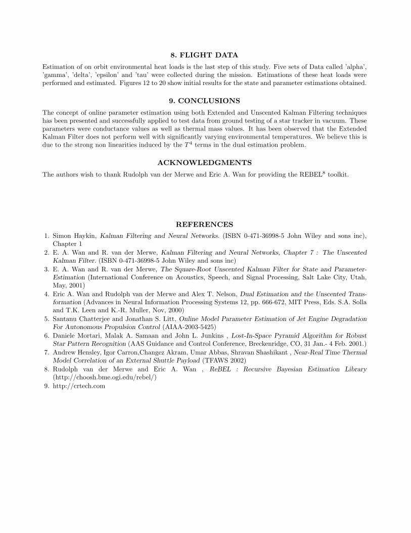
8. FLIGHT DATA
Estimation of on orbit environmental heat loads is the last step of this study. Five sets of Data called ’alpha’,’gamma’, ’delta’, ’epsilon’ and ’tau’ were collected during the mission. Estimations of these heat loads wereperformed and estimated. Figures 12 to 20 show initial results for the state and parameter estimations obtained.
9. CONCLUSIONS
The concept of online parameter estimation using both Extended and Unscented Kalman Filtering techniqueshas been presented and successfully applied to test data from ground testing of a star tracker in vacuum. Theseparameters were conductance values as well as thermal mass values. It has been observed that the ExtendedKalman Filter does not perform well with significantly varying environmental temperatures. We believe this isdue to the strong non linearities induced by the T 4 terms in the dual estimation problem.
ACKNOWLEDGMENTS
The authors wish to thank Rudolph van der Merwe and Eric A. Wan for providing the REBEL8 toolkit.
REFERENCES1. Simon Haykin, Kalman Filtering and Neural Networks. (ISBN 0-471-36998-5 John Wiley and sons inc),
Chapter 12. E. A. Wan and R. van der Merwe, Kalman Filtering and Neural Networks, Chapter 7 : The Unscented
Kalman Filter. (ISBN 0-471-36998-5 John Wiley and sons inc)3. E. A. Wan and R. van der Merwe, The Square-Root Unscented Kalman Filter for State and Parameter-
Estimation (International Conference on Acoustics, Speech, and Signal Processing, Salt Lake City, Utah,May, 2001)
4. Eric A. Wan and Rudolph van der Merwe and Alex T. Nelson, Dual Estimation and the Unscented Trans-formation (Advances in Neural Information Processing Systems 12, pp. 666-672, MIT Press, Eds. S.A. Sollaand T.K. Leen and K.-R. Muller, Nov, 2000)
5. Santanu Chatterjee and Jonathan S. Litt, Online Model Parameter Estimation of Jet Engine DegradationFor Autonomous Propulsion Control (AIAA-2003-5425)
6. Daniele Mortari, Malak A. Samaan and John L. Junkins , Lost-In-Space Pyramid Algorithm for RobustStar Pattern Recognition (AAS Guidance and Control Conference, Breckenridge, CO, 31 Jan.- 4 Feb. 2001.)
7. Andrew Hensley, Igor Carron,Changez Akram, Umar Abbas, Shravan Shashikant , Near-Real Time ThermalModel Correlation of an External Shuttle Payload (TFAWS 2002)
8. Rudolph van der Merwe and Eric A. Wan , ReBEL : Recursive Bayesian Estimation Library(http://choosh.bme.ogi.edu/rebel/)
9. http://crtech.com
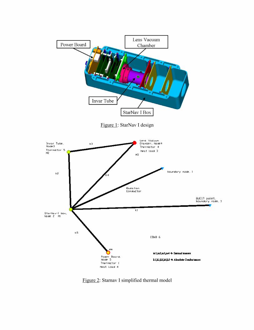
Figure 1: StarNav I design
Figure 2: Starnav I simplified thermal model

Figure 3: Ground Test 1 Estimation using SRUKF
Figure 4: Ground Test 1 Estimation using EKF

Figure 5: Ground Test 2 Estimation using SRUKF
Figure 6: Ground Test 2 Estimation using EKF

Figure 7: Ground Test 3 Estimation using SRUKF
Figure 8: Ground Test 3 Estimation using EKF

Figure 9: Ground Test 4 Estimation using SRUKF
Figure 10: Ground Test 5 Estimation using SRUKF
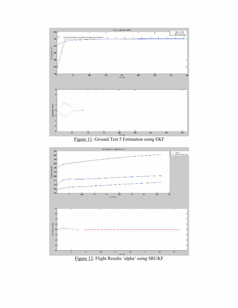
Figure 11: Ground Test 5 Estimation using EKF
Figure 12: Flight Results ‘alpha’ using SRUKF
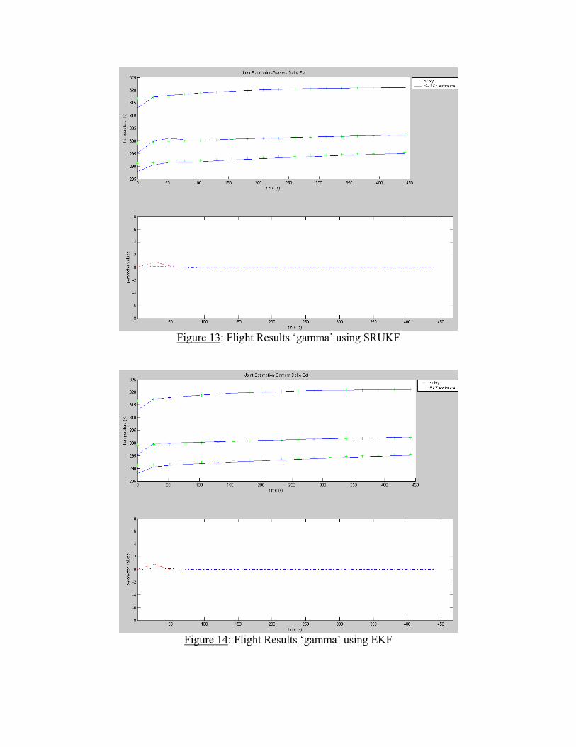
Figure 13: Flight Results ‘gamma’ using SRUKF
Figure 14: Flight Results ‘gamma’ using EKF

Figure 15: Flight Results ‘delta’ using SRUKF
Figure 16: Flight Results ‘delta’ using EKF

Figure 17: Flight Results ‘epsilon’ using SRUKF
Figure 18: Flight Results ‘epsilon’ using EKF

Figure 19: Flight Results ‘tau’ using SRUKF
Figure 20: Flight Results ‘tau’ using EKF