On the Relation Between Flexibility Analysis andRobust Optimization for Linear Systems

Qi Zhanga, Ricardo M. Limab, Ignacio E. Grossmanna,∗

aCenter for Advanced Process Decision-making, Department of Chemical Engineering,Carnegie Mellon University, Pittsburgh, PA 15213, USA

bCenter for Uncertainty Quantification in Computational Science & Engineering,Computer, Electrical and Mathematical Sciences and Engineering Division, King Abdullah

University of Science and Technology, Thuwal 23955-6900, Kingdom of Saudi Arabia

Abstract

Flexibility analysis and robust optimization are two approaches to solving op-

timization problems under uncertainty that share some fundamental concepts,

such as the use of polyhedral uncertainty sets and the worst-case approach to

guarantee feasibility. The connection between these two approaches has not

been sufficiently acknowledged and examined in the literature. In this context,

the contributions of this work are fourfold: (1) a comparison between flexibil-

ity analysis and robust optimization from a historical perspective is presented;

(2) for linear systems, new formulations for the three classical flexibility analy-

sis problems—flexibility test, flexibility index, and design under uncertainty—

based on duality theory and the affinely adjustable robust optimization (AARO)

approach are proposed; (3) the AARO approach is shown to be generally more

restrictive such that it may lead to overly conservative solutions; (4) numeri-

cal examples show the improved computational performance from the proposed

formulations compared to the traditional flexibility analysis models.

∗Corresponding authorEmail address: grossmann@cmu.edu (Ignacio E. Grossmann)

Preprint submitted to Elsevier December 22, 2015

Keywords: Flexibility analysis, robust optimization, optimization under

uncertainty

Introduction

This paper is a tribute to Roger Sargent, the founder and intellectual leader

of the area of process systems engineering (PSE), and his pioneering work on

design of chemical plants with uncertain parameters,1 which has inspired many

of the later works on flexibility analysis and optimal design under uncertainty.

Process flexibility and resiliency analysis of chemical processes using math-

ematical optimization models have received significant attention in the PSE

community for more than thirty years. In general, the study of the flexibility of

a process can be addressed at two stages: (1) at the design stage, where the opti-

mization models for process design explicitly incorporate flexibility constraints,

or (2) when for a fixed design, there is the need to evaluate the process flexibil-

ity in the presence of perturbations of some operating conditions, which at the

design stage were considered constant, but in reality are subject to uncertainty.

In a recent review paper,2 Grossmann et al. give a historical perspective on

the evolution of the concepts and mathematical models used for flexibility anal-

ysis. Some of the earlier works in this area include the work of Friedman and

Reklaitis3,4 from the mid 70s, who proposed techniques for solving linear pro-

gramming (LP) problems with some of the parameters subject to uncertainty;

subsequently from the 80s the resiliency concepts proposed by Saboo et al.5

and applied to heat exchanger networks; and the development of optimization

models to quantify process flexibility by solving the flexibility test and flexibility

2

index problems.6,7

The analysis of the flexibility of chemical processes is closely related to the

solution of optimization problems under uncertainty. In the works mentioned

above, one assumes that each uncertain parameter can take any value within a

given range, and the process is considered sufficiently flexible if feasible operation

can be achieved for the entire parameter range. Interestingly, the exact same

idea forms the foundation of robust optimization,8 which was introduced in

the late 90s. The increasing interest in robust optimization in recent years has

led to many theoretical developments and its application to a wide range of

problems.9,10

The two main concepts shared by flexibility analysis and robust optimization

are the following:

using polyhedral uncertainty sets to describe the uncertainty in the pa-

rameters;

applying worst-case analysis to test feasibility.

However, while the most effective solution approaches developed in flexibility

analysis make use of the Karush-Kuhn-Tucker (KKT) conditions and insights on

the possible sets of active constraints as it is aimed at solving nonlinear models,

robust optimization applies duality theory to linear models to obtain tractable

formulations.

Another major difference between flexibility analysis and “traditional” ro-

bust optimization is the treatment of recourse (reactive actions after the realiza-

tion of the uncertainty). While flexibility analysis explicitly considers control

variables that can adjust depending on the realized values of the uncertain

3

parameters, robust optimization traditionally does not account for recourse,

which often leads to overly conservative solutions. This gap between the two

approaches is being bridged by the recent development of the adjustable robust

optimization concept,11,12 which allows the incorporation of recourse decisions,

typically in the form of linear decision rules.

In this work, we consider a set of linear inequality constraints with a given

general structure for which the following three flexibility analysis problems are

addressed:

1. the flexibility test problem;

2. the flexibility index problem;

3. design under uncertainty with flexibility constraints.

For linear models described by inequalities, we establish the link between flex-

ibility analysis and robust optimization by first developing a new flexibility

analysis approach based on duality. Then, we apply the affinely adjustable ro-

bust optimization11 approach to the same flexibility analysis problems. Hence,

we present and compare the following three approaches:

1. traditional (KKT-based) flexibility analysis (TFA);

2. duality-based flexibility analysis (DFA);

3. affinely adjustable robust optimization (AARO).

While the TFA and DFA approaches lead to mixed-integer linear programming

(MILP) formulations, only LPs need to be solved in the AARO approach. How-

ever, we show that while the TFA and DFA approaches obtain the same optimal

solution, the AARO approach may predict a lower level of flexibility due to the

4

restriction of the recourse to linear functions of the uncertain parameters. The

performance of the different approaches is demonstrated in several numerical

case studies.

The remainder of this paper is organized as follows. In the next section,

we give a historical perspective on flexibility analysis and robust optimization,

which have been developed independently from each other in different research

communities. In the subsequent three sections, the three flexibility analysis

problems are introduced, and for each of them, the formulations resulting from

the three different solution approaches are presented. These formulations are

then applied to three numerical examples. Finally, we close with a summary of

the main results and some concluding remarks.

Historical Perspective

While flexibility analysis was developed in the PSE community, robust opti-

mization is recognized as a subfield of operations research (OR). In the following,

we take a look at the historical development of these two research areas, which

interestingly have evolved almost entirely independently from each other.

In their seminal work from 1975,3,4 Friedman and Reklaitis address the prob-

lem of solving LPs with possibly correlated uncertain parameters, where each

uncertain parameter can take any value within a known range of variation. A

worst-case approach is proposed which aims at finding a solution that is feasible

for any possible realization of the uncertainty. General nonlinear systems are

considered in the work by Grossmann and Sargent from 1978,1 which forms the

basis for all later contributions in the area of flexibility analysis. The major con-

5

ceptual innovation is the distinction between design and control variables; while

design variables are chosen at the design stage and cannot be changed during

the operation of the plant, control variables can be adjusted depending on the

realization of the uncertain parameters. This concept resembles the stage-wise

construction of stochastic programming13 models and realistically represents

the decision-making process in chemical plant design and operation.

Most of the later theoretical work in flexibility analysis was conducted in

the 1980s by Grossmann and coworkers. Halemane and Grossmann6 introduce

a rigorous formulation of the problem of design under uncertainty. A max-

min-max constraint, which involves solving what is known as the flexibility test

problem, guarantees the existence of a feasible region for the specified range of

parameter values. One main result is that if the constraints are convex, the

solution of the flexibility test problem lies at a vertex of the polyhedral region

of parameters. Based on this insight, a vertex enumeration formulation and an

iterative cutting plane algorithm are proposed to solve the design under un-

certainty problem. Swaney and Grossmann7,14 introduce the flexibility index

problem by proposing a quantitative index which measures the size of the pa-

rameter space over which feasible operation can be attained. Two algorithms

have been proposed that are designed to avoid exhaustive vertex enumeration.

Realizing that the flexibility test and flexibility index problems result in bilevel

formulations, Grossmann and Floudas15 replace the lower-level problems by

their KKT conditions and apply an active-constraint strategy to convert the

bilevel problems into single-level mixed-integer problems. The derivation of the

model does not require the assumption of vertex solutions; hence, it is able to

6

predict nonvertex critical points.

Pistikopoulos and Grossmann consider the optimal retrofit design with the

objective of improving process flexibility.16,17 Further extensions include stochas-

tic flexibility,18,19 where the uncertain parameters are described by a joint prob-

ability distribution function; flexibility analysis of dynamic systems;20 flexible

design with confidence intervals and process variability;21,22 new flexibility mea-

sure from constructing feasible polytopes in the parameter space;23 and simpli-

cial approximation of feasibility limits.24,25 More recent works focus on data-

driven approaches for flexibility analysis.26,27,28

While the area of flexibility analysis has evolved over the last 40 years, the

history of robust optimization is very different. The work that is generally rec-

ognized as the first contribution to the area of robust optimization is a short

technical note from 1973 by Soyster,29 who considers robust solutions to LPs

with column-wise uncertainty, which can be seen as a special case of the problem

addressed by Friedman and Reklaitis.3,4 Then, essentially no further develop-

ment was made in the OR community until Soyster’s work was rediscovered in

1998 by Ben-Tal and Nemirovski30 and El Ghaoui et al.,31 who introduced the

notion of uncertainty sets and robust counterparts. While an uncertainty set

is the set of all possible realizations of the uncertainty, a robust counterpart is

a formulation that constraints the original model equations to be feasible for

every possible realization of the uncertainty.

The major concern in robust optimization is computational tractability which

strongly depends on the structure of the optimization problem and the form of

the uncertainty set. Tractable robust counterparts have been derived for a

7

wide variety of optimization problems,8 often by using duality theory. For ex-

ample, the robust counterpart of an LP with uncertain parameters defined by

polyhedral uncertainty sets can be formulated as an LP of similar complex-

ity;32 the robust counterpart of an LP with ellipsoidal uncertainty can be posed

as a second-order cone program (SOCP);32 and for qudratically constrained

quadratic programs (QCQPs) with simple ellipsoidal uncertainty, the robust

counterpart is a semidefinite program (SDP).33 Some of the results for contin-

uous problems can be extended to models with discrete variables.34 For many

other classes of optimization problems, however, only tractable approximate so-

lution approaches have been proposed so far.31,35,36 In particular, obtaining

robust solutions for general nonlinear systems remains a major challenge.

One drawback of robust optimization is that the result may often be overly

conservative since the approach optimizes for the worst case. To address this

issue, Bertsimas and Sim37 introduce the notion of a budget of uncertainty,

which can be changed in order to adjust the level of conservatism in the solution.

In the proposed approach, the budget of uncertainty is encoded in the form of a

cardinality constraint on the number of uncertain parameters that are allowed

to deviate from their nominal values, and probabilistic bounds for constraint

satisfaction as functions of the budget parameter are derived. The concept

of probabilistic guarantees in robust optimization traces back to Ben-Tal and

Nemirovski,38 who show that for an ellipsoid with radius Ω, the corresponding

robust feasible solution satisfies the original constraint with probability at least

1 − e−Ω2/2. Since then, probabilistic guarantees have been derived for a number

of different robust formulations.39,36,40

8

Unlike flexibility analysis, traditional static robust optimization does not

consider recourse, which is another limitation that may lead to overly con-

servative solutions. A more realistic approach has been introduced with the

concept of adjustable/adaptable robust optimization,11,41 which involves ad-

justable recourse decisions that depend on the realization of the uncertainty.

Benders-dual cutting plane42 and column-and-constraint generation43,44 algo-

rithms have been proposed to solve the two-stage robust optimization problem

with fully adjustable recourse. However, solving fully adjustable robust opti-

mization problems is very difficult and in many cases intractable; an effective

way to reduce the computational effort is to describe the recourse decisions as

functions of the uncertain parameters and then restrict these functions to spe-

cific tractable forms. Several classes of recourse functions have been proposed in

the literature,45,46,47 among which the affine or linear decision rules11 are most

popular. While affine decision rules allow the formulation of efficient multistage

models and are shown to be optimal for some specific types of problems,48,49

they generally form a restriction of the fully adjustable case and hence are sub-

optimal. Kuhn et al.12 estimate the approximation error from using linear

decision rules by applying them to both the primal and the dual of the problem.

More recent developments in robust optimization include adjustable robust

optimization with integer recourse50,51,52 and distributionally robust optimiza-

tion,53,54 which addresses the problem of ambiguity in the probability distri-

bution that describes the uncertain parameters. We refer to recent review pa-

pers9,10 for a more comprehensive overview of the advances made by the OR

community in this rapidly growing research area.

9

In recent years, robust optimization has also been applied by the PSE com-

munity, mainly to production scheduling problems55,56,57,58,59,60,61,62 involving

uncertainty in prices, product demands, processing times etc. With only very

few exceptions,63 most works apply the static robust optimization approach

without recourse. Gounaris et al.64 derive robust counterparts for the capaci-

tated vehicle routing problem. Li et al.65 apply robust optimization to linear

and mixed-integer linear optimization problems, and present a systematic study

of the robust counterparts for various uncertainty sets and their geometric rela-

tionships. In a subsequent work, Li et al.66 derive probabilistic guarantees for

constraint satisfaction when applying these robust counterparts.

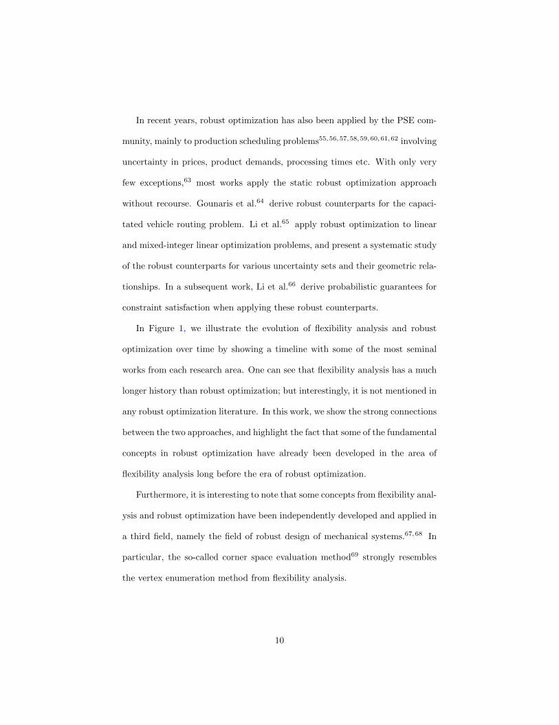
In Figure 1, we illustrate the evolution of flexibility analysis and robust

optimization over time by showing a timeline with some of the most seminal

works from each research area. One can see that flexibility analysis has a much

longer history than robust optimization; but interestingly, it is not mentioned in

any robust optimization literature. In this work, we show the strong connections

between the two approaches, and highlight the fact that some of the fundamental

concepts in robust optimization have already been developed in the area of

flexibility analysis long before the era of robust optimization.

Furthermore, it is interesting to note that some concepts from flexibility anal-

ysis and robust optimization have been independently developed and applied in

a third field, namely the field of robust design of mechanical systems.67,68 In

particular, the so-called corner space evaluation method69 strongly resembles

the vertex enumeration method from flexibility analysis.

10

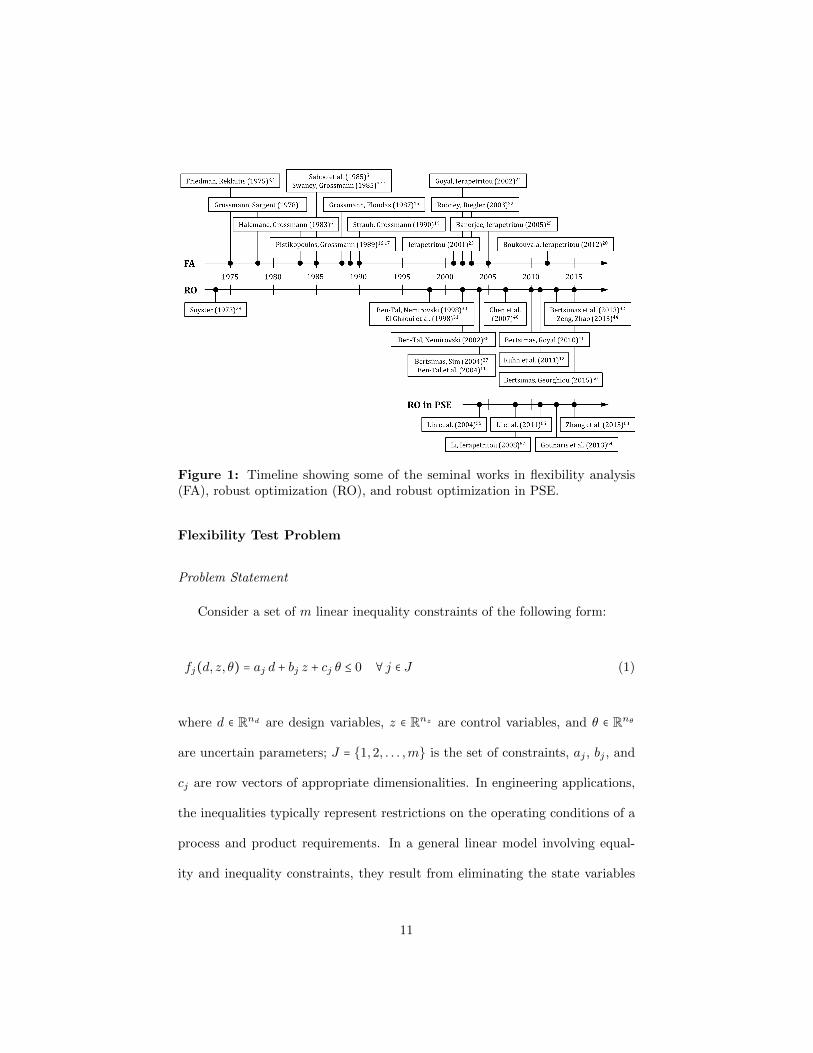
Figure 1: Timeline showing some of the seminal works in flexibility analysis(FA), robust optimization (RO), and robust optimization in PSE.

Flexibility Test Problem

Problem Statement

Consider a set of m linear inequality constraints of the following form:

fj(d, z, θ) = aj d + bj z + cj θ ≤ 0 ∀ j ∈ J (1)

where d ∈ Rnd are design variables, z ∈ Rnz are control variables, and θ ∈ Rnθ

are uncertain parameters; J = 1,2, . . . ,m is the set of constraints, aj , bj , and

cj are row vectors of appropriate dimensionalities. In engineering applications,

the inequalities typically represent restrictions on the operating conditions of a

process and product requirements. In a general linear model involving equal-

ity and inequality constraints, they result from eliminating the state variables

11

from the equations and substituting them in the inequalities. Note that con-

stant summands in the constraint functions can be incorporated in this general

formulation by defining fixed dummy design variables.

The flexibility test problem6 can then be stated as follows: For a given

design d, determine whether by proper adjustment of the control variables z, the

inequalities fj(d, z, θ) ≤ 0, j ∈ J , hold for all θ ∈ T = θ ∶ θL ≤ θ ≤ θU. Here, T

denotes the uncertainty set, which normally takes the form of an nθ-dimensional

hyperbox.

Traditional Flexibility Analysis

For fixed d and θ, the feasibility function is defined as

ψ(d, θ) = minz∈Rnz

maxj∈J

fj(d, z, θ) (2)

which returns the smallest largest fj that can be achieved by adjusting z. If

ψ(d, θ) ≤ 0, we can have feasible operation; if ψ(d, θ) > 0, the operation is

infeasible regardless how we choose z. ψ(d, θ) can be obtained by solving the

following LP:

ψ(d, θ) = minz,u

u

s.t. Ad +B z +C θ ≤ ue

z ∈ Rnz , u ∈ R,

(FF)

where e denotes a column vector of appropriate dimensionality where all entries

are 1.

The flexibility test problem is equivalent to checking whether the maximum

12

value of ψ(d, θ) is less than or equal to zero over the entire range of θ. Hence,

it can be formulated as6

χ(d) = maxθ∈T

ψ(d, θ) = maxθ∈T

minz∈Rnz

maxj∈J

fj(d, z, θ) (FT)

where χ(d) corresponds to the flexibility function of design d with respect to the

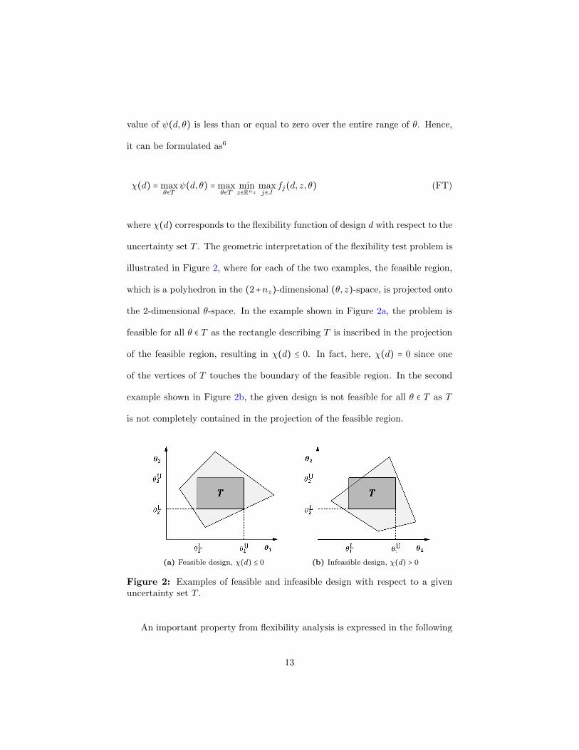
uncertainty set T . The geometric interpretation of the flexibility test problem is

illustrated in Figure 2, where for each of the two examples, the feasible region,

which is a polyhedron in the (2+nz)-dimensional (θ, z)-space, is projected onto

the 2-dimensional θ-space. In the example shown in Figure 2a, the problem is

feasible for all θ ∈ T as the rectangle describing T is inscribed in the projection

of the feasible region, resulting in χ(d) ≤ 0. In fact, here, χ(d) = 0 since one

of the vertices of T touches the boundary of the feasible region. In the second

example shown in Figure 2b, the given design is not feasible for all θ ∈ T as T

is not completely contained in the projection of the feasible region.

(a) Feasible design, χ(d) ≤ 0 (b) Infeasible design, χ(d) > 0

Figure 2: Examples of feasible and infeasible design with respect to a givenuncertainty set T .

An important property from flexibility analysis is expressed in the following

13

theorem.6

Theorem 1. If the constraint functions fj(d, z, θ) are jointly convex in z and

θ, Problem (FT) has its global solution at a vertex of the polyhedral region

T = θ ∶ θL ≤ θ ≤ θU.

In the case of (1), the constraint functions are clearly jointly convex in z

and θ since they only appear linearly in fj . Hence, we can apply Theorem 1

and solve the flexibility test problem by evaluating ψ(d, θ) at all vertices of T .

Based on this property, Swaney and Grossmann14 have proposed two solution

algorithms (direct search and implicit enumeration), which search over the set

of vertices, but are designed to avoid exhaustive enumeration.

The solution approach that we consider here is an active-set method15 that

formulates the flexibility test problem as one single MILP. In this approach,

the flexibility test problem given by Eq. (FT) is posed as a bilevel problem

in which Problem (FF) is the lower-level problem used to compute ψ(d, θ). A

single-level formulation is achieved by replacing the lower-level problem with

its KKT conditions and by modeling the choice of the set of active constraints

with mixed-integer constraints. The resulting flexibility test formulation is as

14

follows:

χ(d) = maxθ,z,u,λ,s,y

u

s.t. Ad +B z +C θ + s = ue

eTλ = 1

BTλ = 0

λ ≤ y

s ≤M(e − y)

eTy ≤ nz + 1

θ ∈ T, z ∈ Rnz , u ∈ R, λ ∈ Rm+, s ∈ Rm

+, y ∈ 0,1m,

(FTTFA)

where s is the vector of slack variables, λ denotes the vector of Lagrange

multipliers, and M is a big-M parameter. Note that Problem (FTTFA) has

3m+nz +2nθ+2 constraints, 2m+nz +nθ+1 continuous variables, and m binary

variables.

Duality-based Flexibility Analysis

We now present an alternative approach, which is derived using LP duality

theory and makes use of Theorem 1. First, we define a new uncertainty set that

only contains the vertices of T :

T = θ ∶ θi = θNi + xi∆θ+i − (1 − xi)∆θ−i , xi ∈ 0,1 ∀ i ∈ Θ (3)

where ∆θ+ = θU−θN, ∆θ− = θN−θL, and Θ = 1,2, . . . , nθ is the set of uncertain

parameters. The vertices are expressed by using the binary variables x. If xi = 1,

15

θi = θUi ; otherwise, θi = θL

i .

The dual of Problem (FF) is

ψ(d, θ) = maxλ

(Ad +C θ)Tλ (4a)

s.t. eTλ = 1 (4b)

−BTλ = 0 (4c)

λ ∈ Rm+, (4d)

where λ is the vector of nonnegative dual variables. Due to strong duality,

Problems (FF) and (4) achieve the same objective function value at the optimal

solution. Hence, the flexibility test problem can be reformulated as:

χ(d) = maxθ∈T

maxλ

(Ad +C θ)Tλ (5a)

s.t. eTλ = 1 (5b)

−BTλ = 0 (5c)

λ ∈ Rm+, (5d)

which is equivalent to Problem (FT) since the optimal solution is guaranteed to

lie at one of the vertices of T . The inner and outer maximization problems can

be merged in order to achieve a single-level problem. We can then rewrite the

objective function as follows:

(Ad +C θ)Tλ = dTATλ + θTCTλ (6a)

= dTATλ + [θN + diag(x)∆θ+ − (I − diag(x))∆θ−]TCTλ (6b)

16

= dTATλ +∑j∈J

cj [θN + diag(x)∆θ+ − (I − diag(x))∆θ−]λj (6c)

= dTATλ +∑j∈J

∑i∈Θ

cji [λj (θNi −∆θ−i ) + λj xi (∆θ+i +∆θ−i )] (6d)

where I is the identity matrix of appropriate dimensionality and diag(⋅) denotes

a diagonal matrix. Note that C is an m × nθ matrix, and while cj denotes the

jth row vector of C, cji is the element at the jth row and ith column of C.

The objective function now contains the bilinear terms λj xi. This bilinearity

can be eliminated by applying exact linearization to the bilinear terms. By doing

so, we obtain the following MILP reformulation of the flexibility test problem:

χ(d) = maxλ,λ,x

dTATλ +∑j∈J

∑i∈Θ

cji [λj (θNi −∆θ−i ) + λij (∆θ+i +∆θ−i )]

s.t. eTλ = 1

−BTλ = 0

λij ≥ (λj − 1) + xi ∀ i ∈ Θ, j ∈ J

λij ≤ λj ∀ i ∈ Θ, j ∈ J

λij ≤ xi ∀ i ∈ Θ, j ∈ J

λ ∈ Rm+, λ ∈ Rnθ×m

+, x ∈ 0,1nθ ,

(FTDFA)

which consists of 3mnθ +nz +1 constraints, m(nθ +1) continuous variables, and

nθ binary variables.

Affinely Adjustable Robust Optimization

In the following, we derive the affinely adjustable robust optimization (AARO)

formulation for the flexibility test problem, and show its relationship to the flexi-

17

bility analysis approach. In particular, we show that the AARO approach can be

overly conservative, i.e. the obtained flexibility function value may be positive

although z can be adjusted such that the design is feasible for all θ ∈ T .

Following a general adjustable robust optimization approach,11 the flexibility

test problem can be formulated as follows:

χ(d) = minz(θ),u∈R

u (7a)

s.t. Ad +B z(θ) +C θ ≤ ue ∀ θ ∈ T, (7b)

where z is expressed as a function of θ since it can be seen as the vector of

recourse variables that are chosen after the realization of the uncertainty. Eq.

(7b) states that all constraints have to be satisfied for every possible realization

of the uncertainty, i.e. for all θ ∈ T .

To show the connection with flexibility analysis, we write Problem (7) equiv-

alently as

χ(d) = minz(θ)

maxθ∈T

maxj∈J

fj(d, z(θ), θ). (8)

The control function z(θ) itself has to be prespecified and cannot be changed

later on, which is why it is a decision made in the outer minimization problem.

Problem (8) is equivalent to Problem (FT) if z(θ) is chosen such that it is the

optimal solution of Problem (FF) for every θ ∈ T .

18

Applying Affine Control Functions

Problem (7) is a semi-infinite program since the number of possible control

functions and the number of possible realizations of the uncertainty are both

infinite. In order to derive a computationally tractable model that still guar-

antees feasibility for all θ ∈ T , we restrict the set of control functions that can

be selected. In static robust optimization, z has to be a constant, which means

that no recourse is allowed. In AARO, z is expressed as an affine function of

θ, i.e. z(θ) = p + Qθ, allowing recourse to a certain extent. Then, instead of

z, p and Q become variables in the formulation. As we will show, it is still a

restriction; however, this is a major improvement compared to the case without

any recourse, and as it turns out, this linear approximation of recourse can of-

ten achieve the same level of flexibility. Substituting the affine function of θ for

z(θ), the restricted flexibility test problem can be formulated as:

χ(d) = minp∈Rnz ,Q∈Rnz×nθ

maxθ∈T

maxj∈J

fj(d, p,Q, θ) (9a)

= minp∈Rnz ,Q∈Rnz×nθ

maxθ∈T

minu∈R

u (9b)

s.t. Ad +B (p +Qθ) +C θ ≤ ue, (9c)

for which we can show the following property:

Proposition 2. Problem (9) has its optimal solution at a vertex of T .

Proof. Problem (9) can be equivalently written as:

χ(d) = minp∈Rnz ,Q∈Rnz×nθ

maxθ∈T

minz,u

u (10a)

19

s.t. Ad +B z +C θ ≤ ue (10b)

z − (p +Qθ) ≤ 0 (10c)

− z + (p +Qθ) ≤ 0 (10d)

z ∈ Rnz , u ∈ R, (10e)

where the affine control function has been incorporated by adding the two in-

equality constraints (10c) and (10d). For any fixed p and Q, the constraint

functions are jointly convex in z and θ. Therefore, according to Theorem 1, the

solution lies at a vertex of T for any p and Q. In particular, this holds true for

the p and Q that minimize the objective function. Hence, Problem (10) has its

optimal solution at a vertex of T , which is equivalently true for Problem (9).

Proposition 2 implies that we only need to consider the vertices of T , of

which there are finitely many. This allows us to obtain χ(d) by solving:

χ(d) = minp,Q,u

u

s.t. Ad +B (p +Qθ) +C θt ≤ ue ∀ t ∈ T

p ∈ Rnz , Q ∈ Rnz×nθ , u ∈ R,

(FTAARO)

where T is the set of vertices of T .

Proposition 3. Let χ(d) and χ(d) be the flexibility function values obtained

from solving Problems (FTTFA) (or alternatively (FTDFA)) and (FTAARO), re-

spectively. Then, χ(d) ≤ χ(d).

Proof. Solving Problem (FTAARO) is equivalent to solving Problem (FTTFA)

20

with the additional constraint z = p + Qθ where p ∈ Rnz , Q ∈ Rnz×nθ . Hence,

(FTAARO) is a restriction of (FTTFA), from which it follows that χ(d) ≤ χ(d).

Proposition 4. For nθ = 1, χ(d) = χ(d).

Proof. Let z1 and z2 be the solutions of Problem (FF) for θ = θL and θ = θU,

respectively. According to Theorem 1, χ(d) will be obtained at one of these two

vertex solutions. By formulating the affine control function

z = [z1 − (z2 − z1)θU − θL

] + ( z2 − z1

θU − θL) θ, (11)

which corresponds to a line in the (1+nz)-dimensional (θ, z)-space, both vertex

solutions can be considered. This implies that when solving Problem (FTAARO),

the same controls (z1 and z2) can be applied at the vertices of T . According

to Proposition 2, χ(d) will be obtained at one of these two vertex solutions.

Hence, χ(d) = χ(d).

Following a similar argument, one arrives at a more general statement:

Proposition 5. If the uncertainty set T is a polytope with nθ + 1 vertices, then

χ(d) = χ(d).

Proof. Suppose z1, z2, . . . , znθ+1 are the solutions of Problem (FF) at the nθ + 1

vertices of T . All nθ + 1 vertex solutions can be expressed through an affine

control function in the form of z = p +Qθ, which represents an nθ-dimensional

hyperplane in the (nθ + nz)-dimensional (θ, z)-space. Thus, the same solution

will be obtained by solving Problems (FTTFA) and (FTAARO). Hence, χ(d) =

21

χ(d).

However, since uncertainty sets in the flexibility analysis problems are hy-

perboxes, Proposition 5 does not apply except in the case of nθ = 1. For nθ ≥ 2,

the number of vertices of the box uncertainty set is greater than nθ + 1. Then,

we may encounter the situation in which not all vertex solutions of the original

flexibility test problem can be expressed by an affine control function. In that

case, the restricted flexibility test formulation (9) may fail in obtaining the same

optimal solution. To formalize this intuitive result, we state the following:

Proposition 6. For nθ ≥ 2, there exist constraint matrices A, B, C, and designs

d such that χ(d) < χ(d).

Proof. We prove this proposition by finding an example for nθ = 2 in which

χ(d) < χ(d). The same result then follows for nθ > 2 since the case of nθ = 2

can be seen as a special case of nθ > 2.

Consider the example with the following four constraints:

f1 = −z ≤ 0 (12a)

f2 = z − θ2 ≤ 0 (12b)

f3 = z − θ1 ≤ 0 (12c)

f4 = −20 − z + θ1 + θ2 ≤ 0 (12d)

which form the polytope that is shown in Figure 3. The uncertainty set is chosen

to be T = (θ1, θ2) ∶ 0 ≤ θ1 ≤ 20, 0 ≤ θ2 ≤ 20.

By solving Problem (FTDFA) for this example, we obtain χ = 0. However,

22

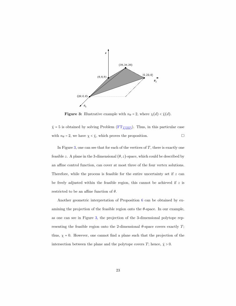
Figure 3: Illustrative example with nθ = 2, where χ(d) < χ(d).

χ = 5 is obtained by solving Problem (FTAARO). Thus, in this particular case

with nθ = 2, we have χ < χ, which proves the proposition.

In Figure 3, one can see that for each of the vertices of T , there is exactly one

feasible z. A plane in the 3-dimensional (θ, z)-space, which could be described by

an affine control function, can cover at most three of the four vertex solutions.

Therefore, while the process is feasible for the entire uncertainty set if z can

be freely adjusted within the feasible region, this cannot be achieved if z is

restricted to be an affine function of θ.

Another geometric interpretation of Proposition 6 can be obtained by ex-

amining the projection of the feasible region onto the θ-space. In our example,

as one can see in Figure 3, the projection of the 3-dimensional polytope rep-

resenting the feasible region onto the 2-dimensional θ-space covers exactly T ;

thus, χ = 0. However, one cannot find a plane such that the projection of the

intersection between the plane and the polytope covers T ; hence, χ > 0.

23

Formulating Robust Counterpart

If T has a large number of vertices, Problem (FTAARO) can quickly become

computationally intractable. In order to avoid enumerating all vertices, we first

notice that the restricted flexibility test problem given by Eq. (9a) can be

equivalently written as follows by interchanging the two inner maximizations:

χ(d) = minp∈Rnz ,Q∈Rnz×nθ

maxj∈J

maxθ∈T

fj(d, p,Q, θ), (13)

from which it follows that we arrive at the same solution by applying a constraint-

wise worst-case approach, i.e. by taking maxθ∈T fj for each individual j ∈ J .

Hence, the restricted flexibility test problem can be reformulated as follows:

χ(d) = minp,Q,u

u (14a)

s.t. aj d + bj p +maxθ∈T

(bj Q + cj) θ ≤ u ∀ j ∈ J (14b)

p ∈ Rnz , Q ∈ Rnz×nθ , u ∈ R. (14c)

Problem (14) is a bilevel problem with m lower-level problems. For each j,

the corresponding lower-level problem is:

maxθ

(bj Q + cj) θ (15a)

s.t. θL ≤ θ ≤ θU, (15b)

24

of which the dual is:

minµj ,νj

(θU)Tµj − (θL)T

νj (16a)

s.t. µj − νj = (bj Q + cj)T(16b)

µj ∈ Rnθ+ , νj ∈ Rnθ+ . (16c)

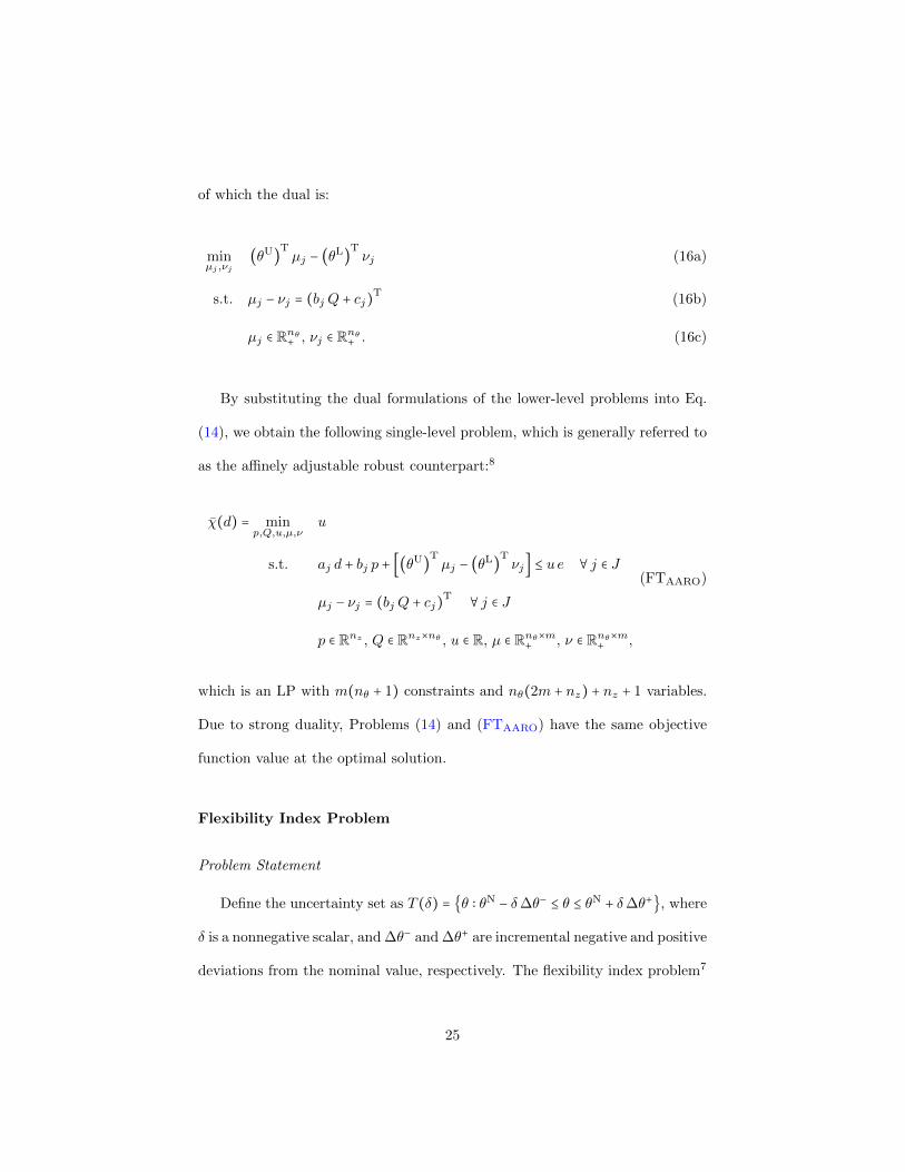
By substituting the dual formulations of the lower-level problems into Eq.

(14), we obtain the following single-level problem, which is generally referred to

as the affinely adjustable robust counterpart:8

χ(d) = minp,Q,u,µ,ν

u

s.t. aj d + bj p + [(θU)Tµj − (θL)T

νj] ≤ ue ∀ j ∈ J

µj − νj = (bj Q + cj)T ∀ j ∈ J

p ∈ Rnz , Q ∈ Rnz×nθ , u ∈ R, µ ∈ Rnθ×m+

, ν ∈ Rnθ×m+

,

(FTAARO)

which is an LP with m(nθ + 1) constraints and nθ(2m + nz) + nz + 1 variables.

Due to strong duality, Problems (14) and (FTAARO) have the same objective

function value at the optimal solution.

Flexibility Index Problem

Problem Statement

Define the uncertainty set as T (δ) = θ ∶ θN − δ∆θ− ≤ θ ≤ θN + δ∆θ+, where

δ is a nonnegative scalar, and ∆θ− and ∆θ+ are incremental negative and positive

deviations from the nominal value, respectively. The flexibility index problem7

25

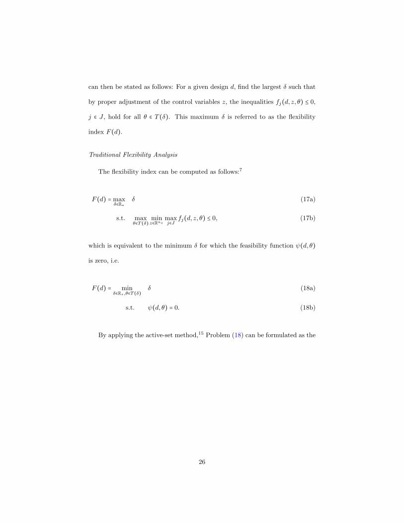
can then be stated as follows: For a given design d, find the largest δ such that

by proper adjustment of the control variables z, the inequalities fj(d, z, θ) ≤ 0,

j ∈ J , hold for all θ ∈ T (δ). This maximum δ is referred to as the flexibility

index F (d).

Traditional Flexibility Analysis

The flexibility index can be computed as follows:7

F (d) = maxδ∈R+

δ (17a)

s.t. maxθ∈T (δ)

minz∈Rnz

maxj∈J

fj(d, z, θ) ≤ 0, (17b)

which is equivalent to the minimum δ for which the feasibility function ψ(d, θ)

is zero, i.e.

F (d) = minδ∈R+,θ∈T (δ)

δ (18a)

s.t. ψ(d, θ) = 0. (18b)

By applying the active-set method,15 Problem (18) can be formulated as the

26

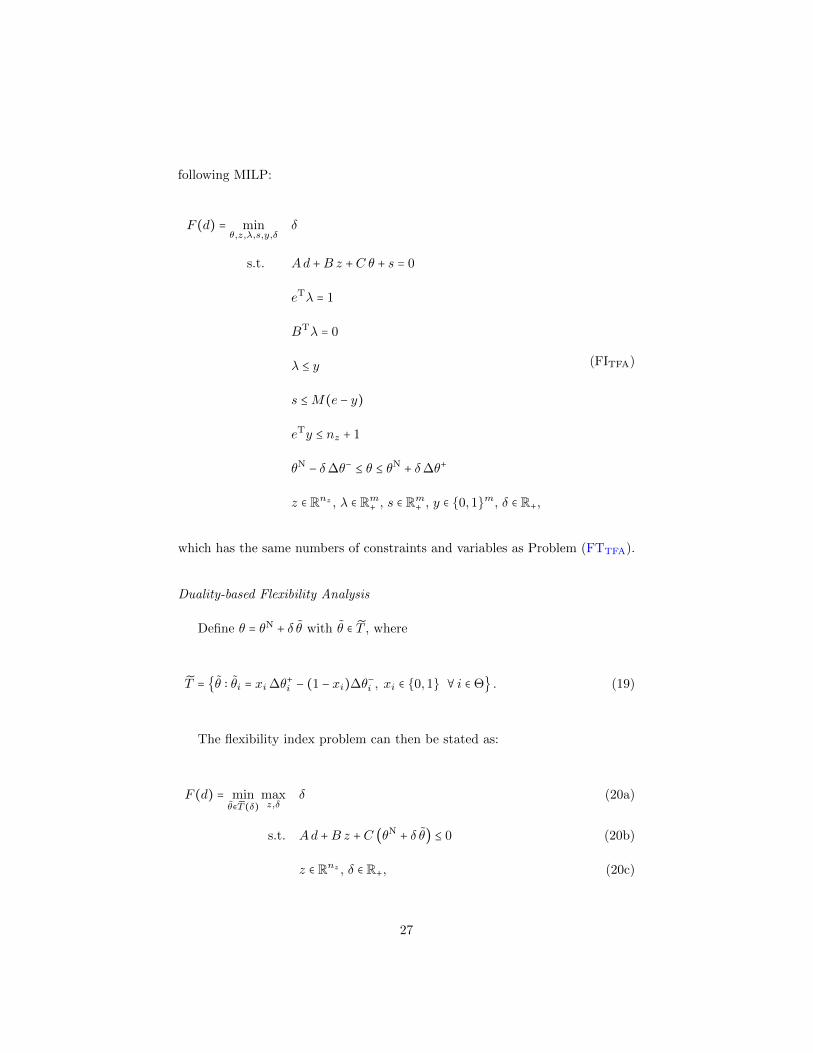
following MILP:

F (d) = minθ,z,λ,s,y,δ

δ

s.t. Ad +B z +C θ + s = 0

eTλ = 1

BTλ = 0

λ ≤ y

s ≤M(e − y)

eTy ≤ nz + 1

θN − δ∆θ− ≤ θ ≤ θN + δ∆θ+

z ∈ Rnz , λ ∈ Rm+, s ∈ Rm

+, y ∈ 0,1m, δ ∈ R+,

(FITFA)

which has the same numbers of constraints and variables as Problem (FTTFA).

Duality-based Flexibility Analysis

Define θ = θN + δ θ with θ ∈ T , where

T = θ ∶ θi = xi∆θ+i − (1 − xi)∆θ−i , xi ∈ 0,1 ∀ i ∈ Θ . (19)

The flexibility index problem can then be stated as:

F (d) = minθ∈T (δ)

maxz,δ

δ (20a)

s.t. Ad +B z +C (θN + δ θ) ≤ 0 (20b)

z ∈ Rnz , δ ∈ R+, (20c)

27

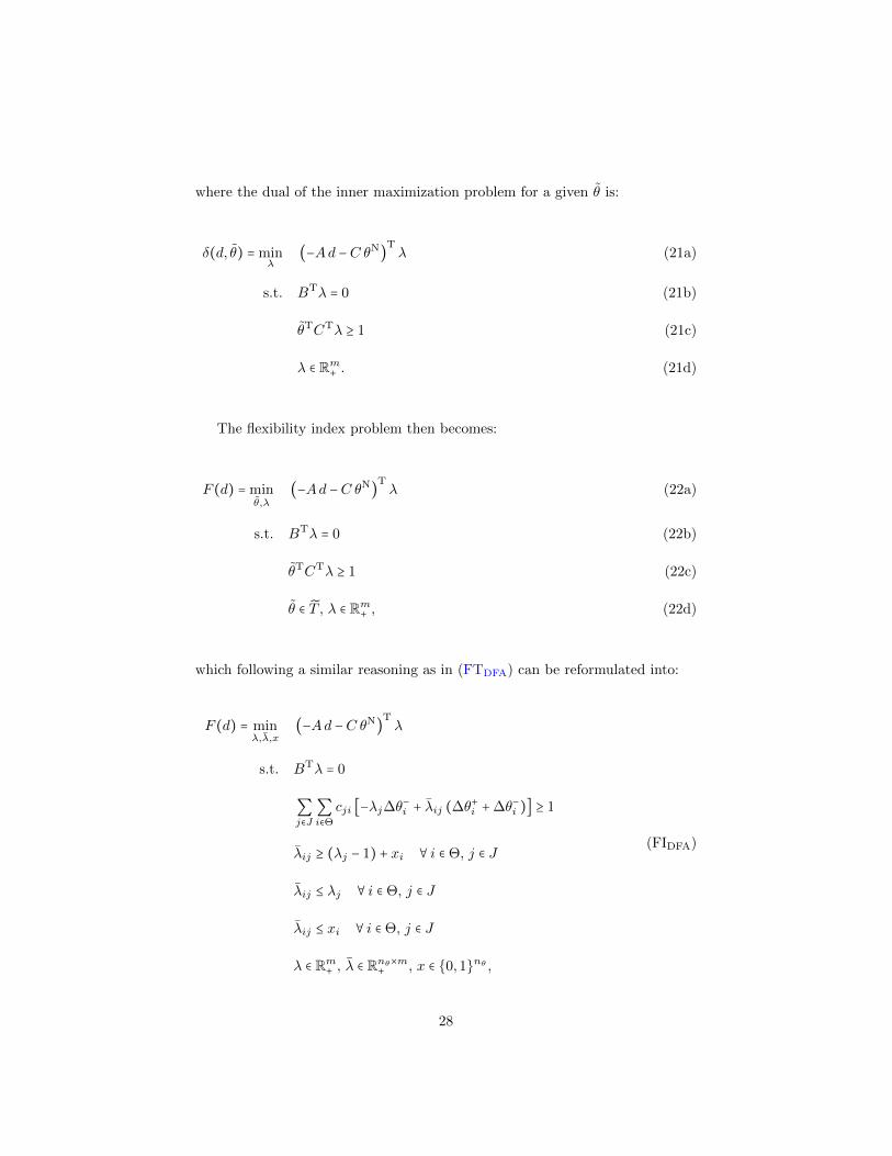
where the dual of the inner maximization problem for a given θ is:

δ(d, θ) = minλ

(−Ad −C θN)Tλ (21a)

s.t. BTλ = 0 (21b)

θTCTλ ≥ 1 (21c)

λ ∈ Rm+. (21d)

The flexibility index problem then becomes:

F (d) = minθ,λ

(−Ad −C θN)Tλ (22a)

s.t. BTλ = 0 (22b)

θTCTλ ≥ 1 (22c)

θ ∈ T , λ ∈ Rm+, (22d)

which following a similar reasoning as in (FTDFA) can be reformulated into:

F (d) = minλ,λ,x

(−Ad −C θN)Tλ

s.t. BTλ = 0

∑j∈J

∑i∈Θ

cji [−λj∆θ−i + λij (∆θ+i +∆θ−i )] ≥ 1

λij ≥ (λj − 1) + xi ∀ i ∈ Θ, j ∈ J

λij ≤ λj ∀ i ∈ Θ, j ∈ J

λij ≤ xi ∀ i ∈ Θ, j ∈ J

λ ∈ Rm+, λ ∈ Rnθ×m

+, x ∈ 0,1nθ ,

(FIDFA)

28

which has the same numbers of constraints and variables as Problem (FTDFA).

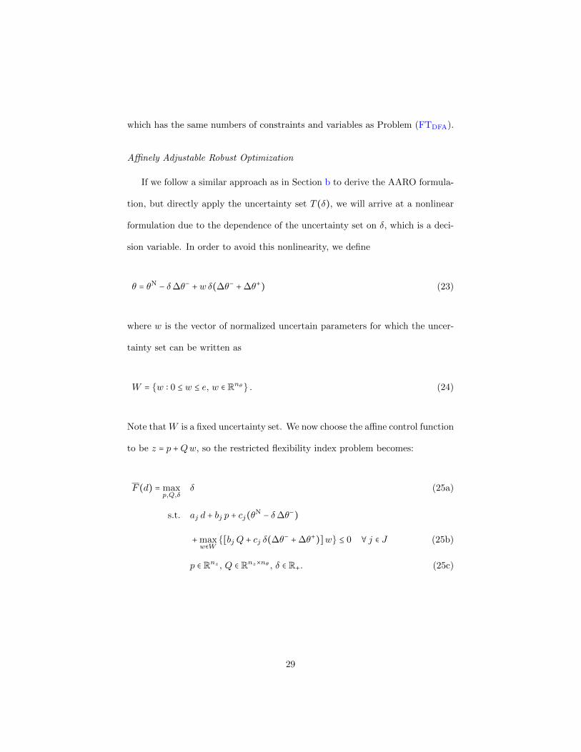
Affinely Adjustable Robust Optimization

If we follow a similar approach as in Section b to derive the AARO formula-

tion, but directly apply the uncertainty set T (δ), we will arrive at a nonlinear

formulation due to the dependence of the uncertainty set on δ, which is a deci-

sion variable. In order to avoid this nonlinearity, we define

θ = θN − δ∆θ− +w δ(∆θ− +∆θ+) (23)

where w is the vector of normalized uncertain parameters for which the uncer-

tainty set can be written as

W = w ∶ 0 ≤ w ≤ e, w ∈ Rnθ . (24)

Note that W is a fixed uncertainty set. We now choose the affine control function

to be z = p +Qw, so the restricted flexibility index problem becomes:

F (d) = maxp,Q,δ

δ (25a)

s.t. aj d + bj p + cj(θN − δ∆θ−)

+maxw∈W

[bj Q + cj δ(∆θ− +∆θ+)]w ≤ 0 ∀ j ∈ J (25b)

p ∈ Rnz , Q ∈ Rnz×nθ , δ ∈ R+. (25c)

29

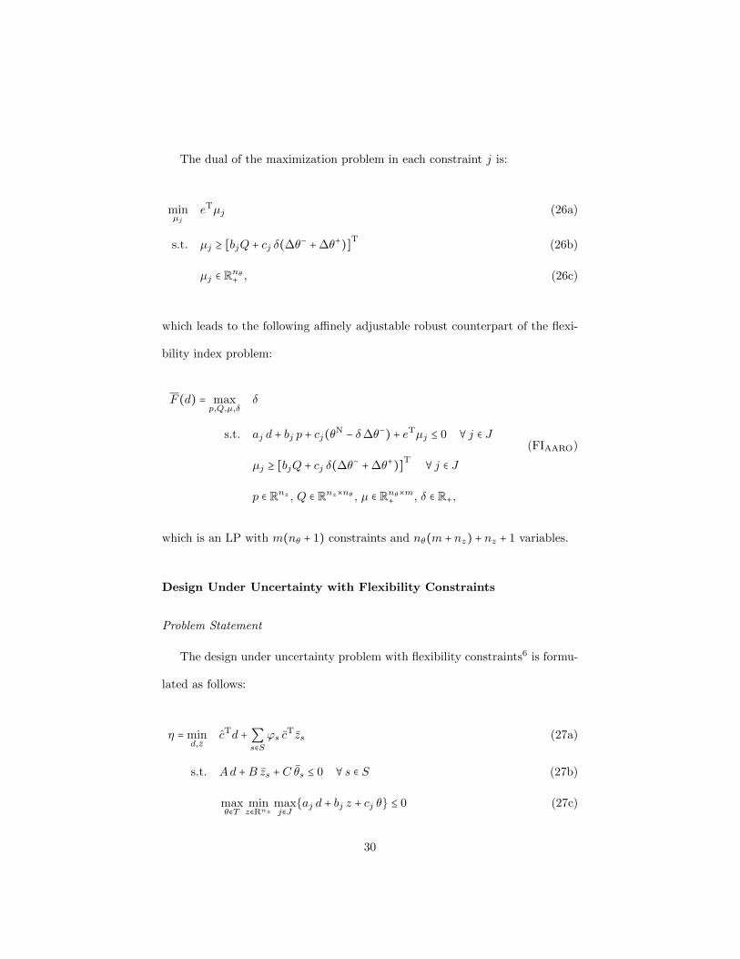
The dual of the maximization problem in each constraint j is:

minµj

eTµj (26a)

s.t. µj ≥ [bjQ + cj δ(∆θ− +∆θ+)]T (26b)

µj ∈ Rnθ+ , (26c)

which leads to the following affinely adjustable robust counterpart of the flexi-

bility index problem:

F (d) = maxp,Q,µ,δ

δ

s.t. aj d + bj p + cj(θN − δ∆θ−) + eTµj ≤ 0 ∀ j ∈ J

µj ≥ [bjQ + cj δ(∆θ− +∆θ+)]T ∀ j ∈ J

p ∈ Rnz , Q ∈ Rnz×nθ , µ ∈ Rnθ×m+

, δ ∈ R+,

(FIAARO)

which is an LP with m(nθ + 1) constraints and nθ(m + nz) + nz + 1 variables.

Design Under Uncertainty with Flexibility Constraints

Problem Statement

The design under uncertainty problem with flexibility constraints6 is formu-

lated as follows:

η = mind,z

cTd +∑s∈S

ϕs cTzs (27a)

s.t. Ad +B zs +C θs ≤ 0 ∀ s ∈ S (27b)

maxθ∈T

minz∈Rnz

maxj∈J

aj d + bj z + cj θ ≤ 0 (27c)

30

d ∈ Rnd , z ∈ Rnz×h, (27d)

where c and c are vectors of cost coefficients. The objective function is an ap-

proximation of the total expected cost, which consists of two parts: the capital

cost associated with the design, cTd, and a scenario-based approximation of the

expected operating cost, ∑s∈S ϕs cTzs. In the scenario set S = 1,2, . . . , h, each

scenario is denoted by the index s and is characterized by θs, the value that the

uncertain parameter θ takes in this particular scenario, and the corresponding

probability ϕs, for which ∑s∈S ϕs = 1. For each scenario, a different control, zs,

is determined, which satisfies Eq. (27b). The expected operating cost is approx-

imated by calculating the sum of the operating costs for the h representative

scenarios in S, each weighted with the corresponding probability.

In addition to Eq. (27b), which ensures that the design is feasible for all

preselected scenarios, the flexibility constraints given by Eq. (27c) further guar-

antee feasibility for all θ ∈ T given that the control variable z can be adjusted

depending on the realization of the uncertain parameter.

Flexibility Analysis

Halemane and Grossmann6 solve Problem (27) with an iterative column-

and-constraint generation approach. The algorithm relies on the fact that a

design is feasible for all θ ∈ T if it is feasible for the worst-case realization of

the uncertainty, which lies at one of the vertices of T . In each iteration, a

relaxation of Problem (27) is solved, where Eq. (27c) is replaced by a set of

constraints of the form fj(d, zt, θt)∀ j ∈ J , where θt is a vertex of T . Then, a

flexibility test is performed for the obtained design. If the design is feasible, the

31

algorithm terminates; otherwise, the critical point (another vertex) obtained

from the flexibility test is added to the formulation, which is solved in the next

iteration to determine the next design suggestion. The complete algorithm is as

follows:

Step 1 Set k = 0. Choose an initial set T0 consisting of N0 critical points.

Step 2 Solve the following problem:

mind,z,z

cTd +∑s∈S

ϕs cTzs (28a)

s.t. Ad +B zs +C θs ≤ 0 ∀ s ∈ S (28b)

Ad +B zt +C θt ≤ 0 ∀ t ∈ Tk (28c)

d ∈ Rnd , z ∈ Rnz×h, z ∈ Rn×Nk (28d)

to obtain design dk.

Step 3 Solve Problem (FTTFA) or (FTDFA) by setting d = dk, and obtain

critical point θck. If χ(dk) ≤ 0, stop; otherwise, go to Step 4.

Step 4 Set θk+1 = θck, Nk+1 = Nk + 1, and define Tk+1 = 1,2, . . . ,Nk+1. Set

k = k + 1 and go to Step 2.

The algorithm converges in a finite number of iterations since there is a finite

number of vertices. Note that the only difference between the traditional and

the duality-based flexibility analysis approaches is the flexibility test problem

that is solved in Step 3.

There are different approaches for choosing the initial set of critical points

T0. For example, one effective strategy1 is to determine the critical points

32

for each constraint by examining the signs of the coefficients in matrix C and

use these points as the initial set. For the remainder of the paper, we refer

to the variant of the algorithm applying this initialization strategy as DF∗

TFA

or DF∗

DFA (depending on whether the TFA or DFA flexibility test problem is

solved). Alternatively, one could also simply let T0 be empty; this variant of

the algorithm will be denoted by DF0TFA or DF0

DFA.

It is worth mentioning that very recently, similar column-and-constraint gen-

eration algorithms have been proposed to solve the two-stage robust optimiza-

tion problem that allows full adjustability in the recourse.43,44 This is just

another indicator for the strong connection between flexibility analysis and ro-

bust optimization, and example of the pioneering work in flexibility analysis

that has long preceded the era of robust optimization.

Affinely Adjustable Robust Optimization

Unlike the flexibility analysis approach, the AARO approach does not require

an iterative framework. Here, we only need to solve a single LP. In order to

obtain the AARO formulation, we simply take Problem (FTAARO), set u = 0

to ensure feasibility, and add Eqs. (27a) and (27b) to describe the objective

33

function. Hence, we arrive at the following formulation:

η = mind,z,p,Q,µ,ν

cTd +∑s∈S

ϕs cTzs

s.t. Ad +B zs +C θs ≤ 0 ∀ s ∈ S

aj d + bj p + [(θU)Tµj − (θL)T

νj] ≤ 0 ∀ j ∈ J

µj − νj = (bj Q + cj)T ∀ j ∈ J

d ∈ Rnd , z ∈ Rnz×h, p ∈ Rnz , Q ∈ Rnz×nθ , µ ∈ Rnθ×m+

, ν ∈ Rnθ×m+

.

(DFAARO)

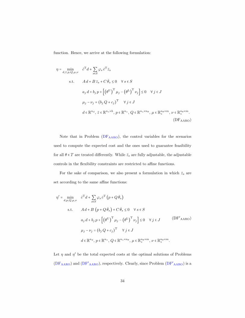
Note that in Problem (DFAARO), the control variables for the scenarios

used to compute the expected cost and the ones used to guarantee feasibility

for all θ ∈ T are treated differently. While zs are fully adjustable, the adjustable

controls in the flexibility constraints are restricted to affine functions.

For the sake of comparison, we also present a formulation in which zs are

set according to the same affine functions:

η′ = mind,p,Q,µ,ν

cTd +∑s∈S

ϕs cT (p +Qθs)

s.t. Ad +B (p +Qθs) +C θs ≤ 0 ∀ s ∈ S

aj d + bj p + [(θU)Tµj − (θL)T

νj] ≤ 0 ∀ j ∈ J

µj − νj = (bj Q + cj)T ∀ j ∈ J

d ∈ Rnd , p ∈ Rnz , Q ∈ Rnz×nθ , µ ∈ Rnθ×m+

, ν ∈ Rnθ×m+

.

(DF′

AARO)

Let η and η′ be the total expected costs at the optimal solutions of Problems

(DFAARO) and (DF′

AARO), respectively. Clearly, since Problem (DF′

AARO) is a

34

restriction of Problem (DFAARO), η ≤ η′. The advantage of Problem (DF′

AARO)

is that it does not involve the variables zs, which, however, usually does not

translate into significant reductions in computational times.

Numerical Examples

In the following, we apply the proposed models to flexibility analysis prob-

lems for three different examples. While the first two examples are meant to be

illustrative, the third one is significantly larger in size and allows more insights

into the computational performance of the different approaches. All models

were implemented in GAMS 24.4.1,70 and the commercial solver CPLEX 12.6.1

was applied to solve the LPs and MILPs on an Intel® CoreTM i7-2600 machine

at 3.40 GHz with 8 hardware threads and 8 GB RAM running Windows 7 Pro-

fessional. Unless specified otherwise, the LPs were solved with the concurrent

option using all 8 threads. Similarly, MILPs were also solved in parallel using

all available threads.

Example 1: Heat Exchanger Network

This first example of a small heat exchanger network (HEN) is based on an

example introduced by Grossmann and Floudas.15 The HEN consisting of two

hot streams, two cold streams, three heat exchangers and one cooler is shown

in Figure 4. Here, the uncertainty lies in the inlet temperatures of the hot and

cold streams; hence, the four uncertain parameters are T1, T3, T5, and T8. The

nominal values for the uncertain temperatures are shown in Figure 4, and the

maximum deviations from the nominal values for each temperature are assumed

35

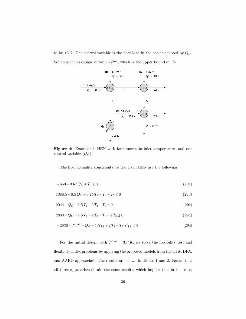
to be ±5 K. The control variable is the heat load in the cooler denoted by QC .

We consider as design variable Tmax7 , which is the upper bound on T7.

Figure 4: Example 1, HEN with four uncertain inlet temperatures and onecontrol variable (QC).

The five inequality constraints for the given HEN are the following:

− 350 − 0.67QC + T3 ≤ 0 (29a)

1388.5 + 0.5QC − 0.75T1 − T3 − T5 ≤ 0 (29b)

2044 +QC − 1.5T1 − 2T3 − T5 ≤ 0 (29c)

2830 +QC − 1.5T1 − 2T3 − T5 − 2T8 ≤ 0 (29d)

− 2830 − Tmax7 −QC + 1.5T1 + 2T3 + T5 + T8 ≤ 0 (29e)

For the initial design with Tmax7 = 317 K, we solve the flexibility test and

flexibility index problems by applying the proposed models from the TFA, DFA,

and AARO approaches. The results are shown in Tables 1 and 2. Notice that

all three approaches obtain the same results, which implies that in this case,

36

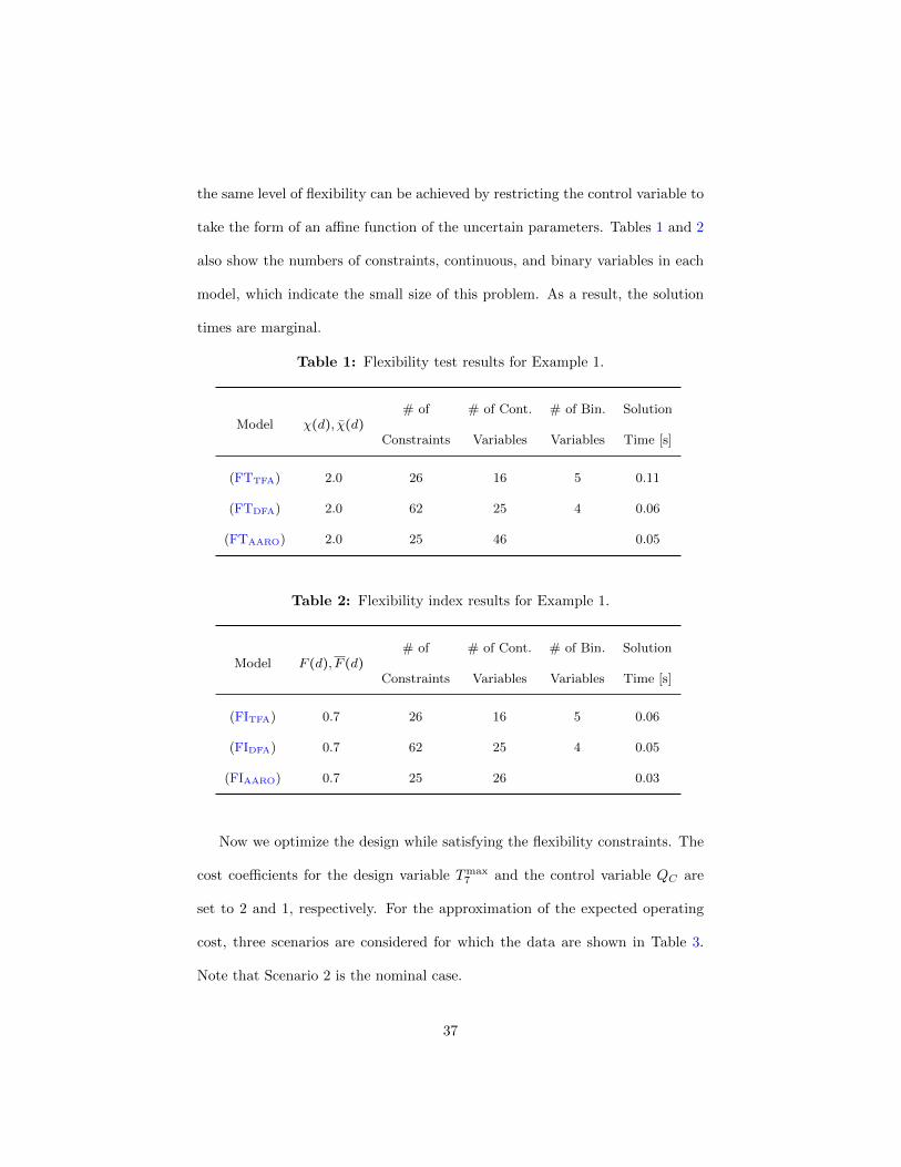
the same level of flexibility can be achieved by restricting the control variable to

take the form of an affine function of the uncertain parameters. Tables 1 and 2

also show the numbers of constraints, continuous, and binary variables in each

model, which indicate the small size of this problem. As a result, the solution

times are marginal.

Table 1: Flexibility test results for Example 1.

Model χ(d), χ(d)# of # of Cont. # of Bin. Solution

Constraints Variables Variables Time [s]

(FTTFA) 2.0 26 16 5 0.11

(FTDFA) 2.0 62 25 4 0.06

(FTAARO) 2.0 25 46 0.05

Table 2: Flexibility index results for Example 1.

Model F (d), F (d)# of # of Cont. # of Bin. Solution

Constraints Variables Variables Time [s]

(FITFA) 0.7 26 16 5 0.06

(FIDFA) 0.7 62 25 4 0.05

(FIAARO) 0.7 25 26 0.03

Now we optimize the design while satisfying the flexibility constraints. The

cost coefficients for the design variable Tmax7 and the control variable QC are

set to 2 and 1, respectively. For the approximation of the expected operating

cost, three scenarios are considered for which the data are shown in Table 3.

Note that Scenario 2 is the nominal case.

37

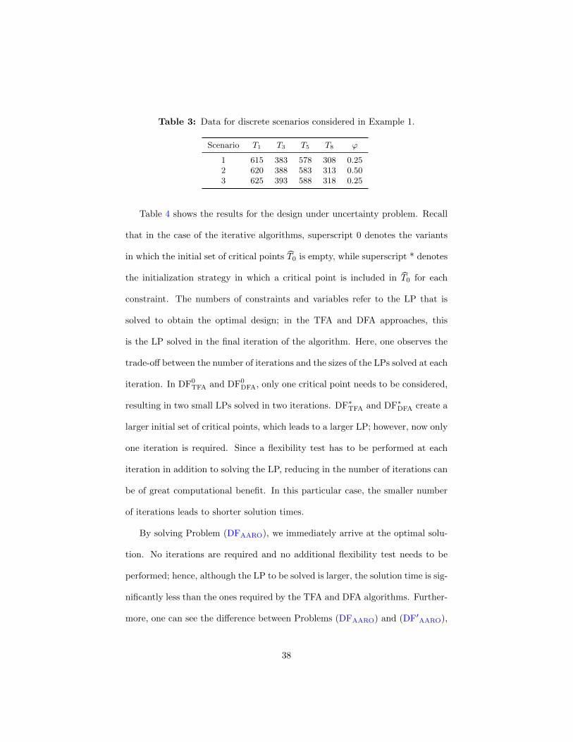
Table 3: Data for discrete scenarios considered in Example 1.

Scenario T1 T3 T5 T8 ϕ

1 615 383 578 308 0.252 620 388 583 313 0.503 625 393 588 318 0.25

Table 4 shows the results for the design under uncertainty problem. Recall

that in the case of the iterative algorithms, superscript 0 denotes the variants

in which the initial set of critical points T0 is empty, while superscript * denotes

the initialization strategy in which a critical point is included in T0 for each

constraint. The numbers of constraints and variables refer to the LP that is

solved to obtain the optimal design; in the TFA and DFA approaches, this

is the LP solved in the final iteration of the algorithm. Here, one observes the

trade-off between the number of iterations and the sizes of the LPs solved at each

iteration. In DF0TFA and DF0

DFA, only one critical point needs to be considered,

resulting in two small LPs solved in two iterations. DF∗

TFA and DF∗

DFA create a

larger initial set of critical points, which leads to a larger LP; however, now only

one iteration is required. Since a flexibility test has to be performed at each

iteration in addition to solving the LP, reducing in the number of iterations can

be of great computational benefit. In this particular case, the smaller number

of iterations leads to shorter solution times.

By solving Problem (DFAARO), we immediately arrive at the optimal solu-

tion. No iterations are required and no additional flexibility test needs to be

performed; hence, although the LP to be solved is larger, the solution time is sig-

nificantly less than the ones required by the TFA and DFA algorithms. Further-

more, one can see the difference between Problems (DFAARO) and (DF′

AARO),

38

Table 4: Design under uncertainty results for Example 1.

Model/ Expected # of # of # of Cont. SolutionAlgorithm Cost Iterations Constraints Variables Time [s]

DF0TFA 724 2 20 5 0.47

DF∗TFA 724 1 30 7 0.23DF0

DFA 724 2 20 5 0.49DF∗DFA 724 1 30 7 0.24

(DFAARO) 724 40 49 0.10(DF′AARO) 727 40 46 0.09

where the latter leads to a slightly higher total expected cost due to the restric-

tion of the control variable to an affine function also in the three scenarios used

to compute the expected cost.

Example 2: Process Flowsheet

Consider the simple process flowsheet shown in Figure 5. In this process,

Material A is fed into a reactor where it reacts to Materials B and C at a fixed

conversion ratio ξ. Materials B and C are then separated in an ideal separator

in order to satisfy product demands DB and DC . Here, the uncertainty lies in

the demands and in the effective geometries of the inlet pipe and of the reactor,

which have an impact on the flow capacities in the pipe and the reactor. The

geometric properties of the pipe and the reactor are represented by the charac-

teristic numbers R and V , respectively; these parameters may be uncertain due

to fouling or wear and tear. The control variable here is the feed flowrate mA.

The given process is represented by the following inequality constraints:

−mA + 0.2V ≤ 0 (30a)

mA − V ≤ 0 (30b)

39

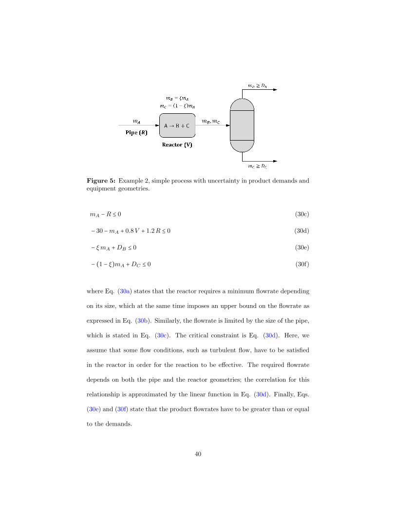
Figure 5: Example 2, simple process with uncertainty in product demands andequipment geometries.

mA −R ≤ 0 (30c)

− 30 −mA + 0.8V + 1.2R ≤ 0 (30d)

− ξmA +DB ≤ 0 (30e)

− (1 − ξ)mA +DC ≤ 0 (30f)

where Eq. (30a) states that the reactor requires a minimum flowrate depending

on its size, which at the same time imposes an upper bound on the flowrate as

expressed in Eq. (30b). Similarly, the flowrate is limited by the size of the pipe,

which is stated in Eq. (30c). The critical constraint is Eq. (30d). Here, we

assume that some flow conditions, such as turbulent flow, have to be satisfied

in the reactor in order for the reaction to be effective. The required flowrate

depends on both the pipe and the reactor geometries; the correlation for this

relationship is approximated by the linear function in Eq. (30d). Finally, Eqs.

(30e) and (30f) state that the product flowrates have to be greater than or equal

to the demands.

40

We solve the flexibility test and flexibility index problems for ξ = 0.6 and

the following uncertainty sets: DB ∈ [6,8], DC ∈ [3,5], R ∈ [15,25], and V ∈

[14,26]. In the nominal case, each uncertain parameter takes the value of the

midpoint in the corresponding uncertainty range. The results are shown in

Table 5. One can see that the flexibility analysis and AARO approaches obtain

different solutions, namely χ(d) < χ(d) and F (d) > F (d), which is due to the

restriction of the control variable to affine functions in the AARO models. In

this case, the TFA and DFA models correctly report that the process is feasible

for every possible realization of the uncertainty given that the feed flowrate can

be properly adjusted, while the AARO model fails to do so. Note that we do

not report computational results due to the small problem sizes and marginal

solution times as was the case in Example 1.

Table 5: Flexibility test and flexibility index results for Example 2.

Approach χ(d), χ(d) F (d), F (d)

TFA/DFA −0.25 1.09AARO 1.10 0.78

Example 3: Planning of Large-Scale Process Network

In this example, we consider the long-term production planning of a large-

scale process network representing a petrochemical complex.71 The given pro-

cess network, which is schematically shown in Figure 6, consists of 38 processes

and 28 chemicals. The planning model is shown in the following. Note that

the nomenclature for this model is independent from and therefore not to be

confused with the one used for the models presented in the previous sections.

41

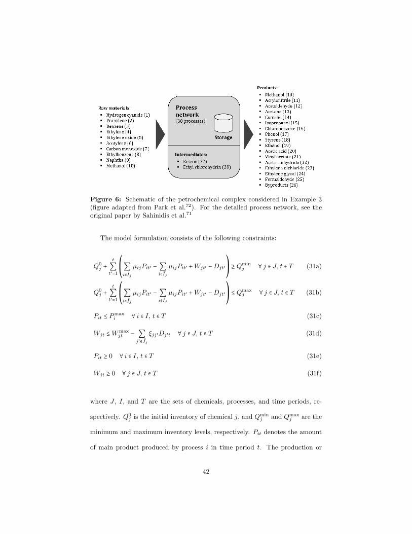
Figure 6: Schematic of the petrochemical complex considered in Example 3(figure adapted from Park et al.72). For the detailed process network, see theoriginal paper by Sahinidis et al.71

The model formulation consists of the following constraints:

Q0j +

t

∑t′=1

⎛⎜⎝∑i∈Ij

µijPit′ − ∑i∈Ij

µijPit′ +Wjt′ −Djt′

⎞⎟⎠≥ Qmin

j ∀ j ∈ J, t ∈ T (31a)

Q0j +

t

∑t′=1

⎛⎜⎝∑i∈Ij

µijPit′ − ∑i∈Ij

µijPit′ +Wjt′ −Djt′

⎞⎟⎠≤ Qmax

j ∀ j ∈ J, t ∈ T (31b)

Pit ≤ Pmaxi ∀ i ∈ I, t ∈ T (31c)

Wjt ≤Wmaxjt − ∑

j′∈Jj

ξjj′Dj′t ∀ j ∈ J, t ∈ T (31d)

Pit ≥ 0 ∀ i ∈ I, t ∈ T (31e)

Wjt ≥ 0 ∀ j ∈ J, t ∈ T (31f)

where J , I, and T are the sets of chemicals, processes, and time periods, re-

spectively. Q0j is the initial inventory of chemical j, and Qmin

j and Qmaxj are the

minimum and maximum inventory levels, respectively. Pit denotes the amount

of main product produced by process i in time period t. The production or

42

consumption of chemical j by process i is given by a conversion factor, denoted

by µij , with respect to the main product; hence, µijPit is the amount of chem-

ical j that is produced or consumed by process i in time period t. The sets

of processes producing and consuming chemical j are denoted by Ij and Ij ,

respectively. Wjt denotes the amount of chemical j purchased, and Djt is the

demand for chemical j in time period t.

Eqs. (31a) and (31b) are the inventory constraints, which ensure that the

inventory level is within the given bounds at any time. Eq. (31c) sets the

production capacity for each process. In Eq. (31d), the assumption is that

the purchase limit for chemical j depends on the demand for products that

require chemical j as feed, which is represented by the set of products Jj . The

intuition is that the higher the market demand is for products requiring feed j,

the more limited will the availability of chemical j be. Here, the coefficient ξjj′

defines how much the purchase limit for chemical j is affected by the demand

of chemical j′ ∈ Jj . Eqs. (31e) and (31f) are nonnegativity constraints.

In this model, Q0j , Q

minj , Wmax

jt , µij , and ξjj′ are fixed constants, Qmaxj and

Pmaxi are the design variables, and Pit and Wjt are the control variables. The

uncertainty lies in the demand, i.e. the uncertain parameters are Djt of which

there exist 16 for each time period.

In the following, we apply the proposed models to problem instances of dif-

ferent sizes, which are created by varying the number of time periods, NT . The

computational time limit for each problem is set to one hour (wall-clock time).

The flexibility test and flexibility index problems are solved for a particular

design, i.e. for specific fixed values of Qmaxj and Pmax

i ; the results are shown

43

in Tables 6 and 7. In order to provide an indicator for the tightness of each

MILP formulation, we show both vMIP and vRMIP, which denote the objective

function values at the optimal solutions of the MILP and its LP relaxation,

respectively. Note that the interpretation of vMIP varies between the different

problems; while it may refer to χ(d) or χ(d) in the flexibility test problems or

to F (d) or F (d) in the flexibility index problems, it may also be none of those

if the MILP is not solved to optimality. The solutions of the AARO LP models

are also listed in the vMIP-column. Furthermore, the relative optimality gap (as

defined in CPLEX) is shown for each MILP. From the computational results,

we make the following observations:

In almost all instances, the DFA and the AARO models obtained the same

optimal solution. The only exception is the flexibility index problem for

NT = 10, where Problem (FIDFA) was not solved to optimality. The TFA

approach only solved the flexibility test problem for NT = 1 to optimality

within the given time limit; in all other instances, the TFA models failed

to find the optimal solution or in some cases even a feasible solution (see

flexibility test for NT = 8 and NT = 10).

For the larger instances, the time required by the AARO LP models to

solve the flexibility test and flexibility index problems was often about one

order of magnitude shorter than the time required by the DFA models.

Compared to the DFA and AARO models, the TFA models exhibit signif-

icantly smaller numbers of constraints and continuous variables. However,

recall that the TFA MILP models have m binary variables, while the DFA

44

MILP models have nθ binary variables; since there are considerably more

constraints than uncertain parameters in this problem, the TFA models

have larger numbers of binary variables.

The comparison between the vRMIP-values of the TFA and DFA models

indicates that the TFA models have significantly weaker relaxations, in

part because of the big-M constraints. This is the primary reason for the

better computational performance of the tighter DFA MILP models.

It should be mentioned that although in many instances, vRMIP = vMIP

for the DFA models, it is often the case that the LP relaxation does not

result in an integer solution. In such a case, the problem does not solve

at the root node and further branching is needed.

In all instances, when solving the flexibility index problem using formula-

tion (FITFA), the lower bound did not improve (i.e. remained zero) during

the branch-and-bound process, even when a depth-first branching strat-

egy was applied. This observation implies that there is sufficient flexibility

in the model such that even with only one binary variable being relaxed,

there exists a feasible solution with δ = 0. This special structure of the

problem has the consequence that a very large number of nodes in the

branch-and-bound tree have to be examined in order to prove optimality.

45

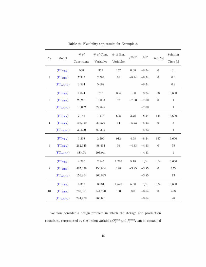
Table 6: Flexibility test results for Example 3.

NT Model# of # of Cont. # of Bin.

vRMIP vMIP Gap [%]Solution

Constraints Variables Variables Time [s]

1

(FTTFA) 538 369 152 0.68 −8.24 0 31

(FTDFA) 7,345 2,584 16 −8.24 −8.24 0 0.3

(FTAARO) 2,584 5,682 −8.24 0.2

2

(FTTFA) 1,074 737 304 1.98 −8.24 58 3,600

(FTDFA) 29,281 10,033 32 −7.00 −7.00 0 1

(FTAARO) 10,032 22,625 −7.00 1

4

(FTTFA) 2,146 1,473 608 3.78 −8.24 146 3,600

(FTDFA) 116,929 39,520 64 −5.23 −5.23 0 3

(FTAARO) 39,520 90,305 −5.23 1

6

(FTTFA) 3,218 2,209 912 4.68 −8.24 157 3,600

(FTDFA) 262,945 88,464 96 −4.33 −4.33 0 55

(FTAARO) 88,464 203,041 −4.33 5

8

(FTTFA) 4,290 2,945 1,216 5.18 n/a n/a 3,600

(FTDFA) 467,329 156,864 128 −3.85 −3.85 0 155

(FTAARO) 156,864 360,833 −3.85 13

10

(FTTFA) 5,362 3,681 1,520 5.38 n/a n/a 3,600

(FTDFA) 730,081 244,720 160 8.0 −3.64 0 468

(FTAARO) 244,720 563,681 −3.64 26

We now consider a design problem in which the storage and production

capacities, represented by the design variables Qmaxj and Pmax

i , can be expanded

46

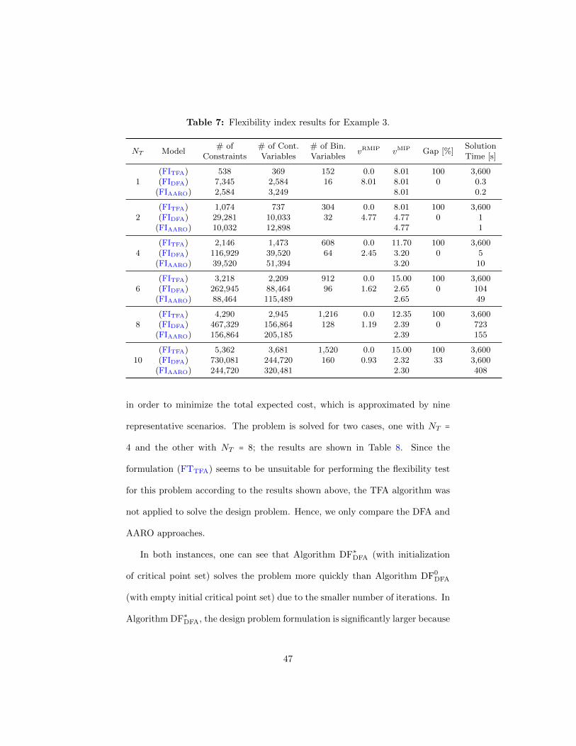
Table 7: Flexibility index results for Example 3.

NT Model# of # of Cont. # of Bin.

vRMIP vMIP Gap [%]Solution

Constraints Variables Variables Time [s]

1(FITFA) 538 369 152 0.0 8.01 100 3,600(FIDFA) 7,345 2,584 16 8.01 8.01 0 0.3

(FIAARO) 2,584 3,249 8.01 0.2

2(FITFA) 1,074 737 304 0.0 8.01 100 3,600(FIDFA) 29,281 10,033 32 4.77 4.77 0 1

(FIAARO) 10,032 12,898 4.77 1

4(FITFA) 2,146 1,473 608 0.0 11.70 100 3,600(FIDFA) 116,929 39,520 64 2.45 3.20 0 5

(FIAARO) 39,520 51,394 3.20 10

6(FITFA) 3,218 2,209 912 0.0 15.00 100 3,600(FIDFA) 262,945 88,464 96 1.62 2.65 0 104

(FIAARO) 88,464 115,489 2.65 49

8(FITFA) 4,290 2,945 1,216 0.0 12.35 100 3,600(FIDFA) 467,329 156,864 128 1.19 2.39 0 723

(FIAARO) 156,864 205,185 2.39 155

10(FITFA) 5,362 3,681 1,520 0.0 15.00 100 3,600(FIDFA) 730,081 244,720 160 0.93 2.32 33 3,600

(FIAARO) 244,720 320,481 2.30 408

in order to minimize the total expected cost, which is approximated by nine

representative scenarios. The problem is solved for two cases, one with NT =

4 and the other with NT = 8; the results are shown in Table 8. Since the

formulation (FTTFA) seems to be unsuitable for performing the flexibility test

for this problem according to the results shown above, the TFA algorithm was

not applied to solve the design problem. Hence, we only compare the DFA and

AARO approaches.

In both instances, one can see that Algorithm DF∗

DFA (with initialization

of critical point set) solves the problem more quickly than Algorithm DF0DFA

(with empty initial critical point set) due to the smaller number of iterations. In

Algorithm DF∗

DFA, the design problem formulation is significantly larger because

47

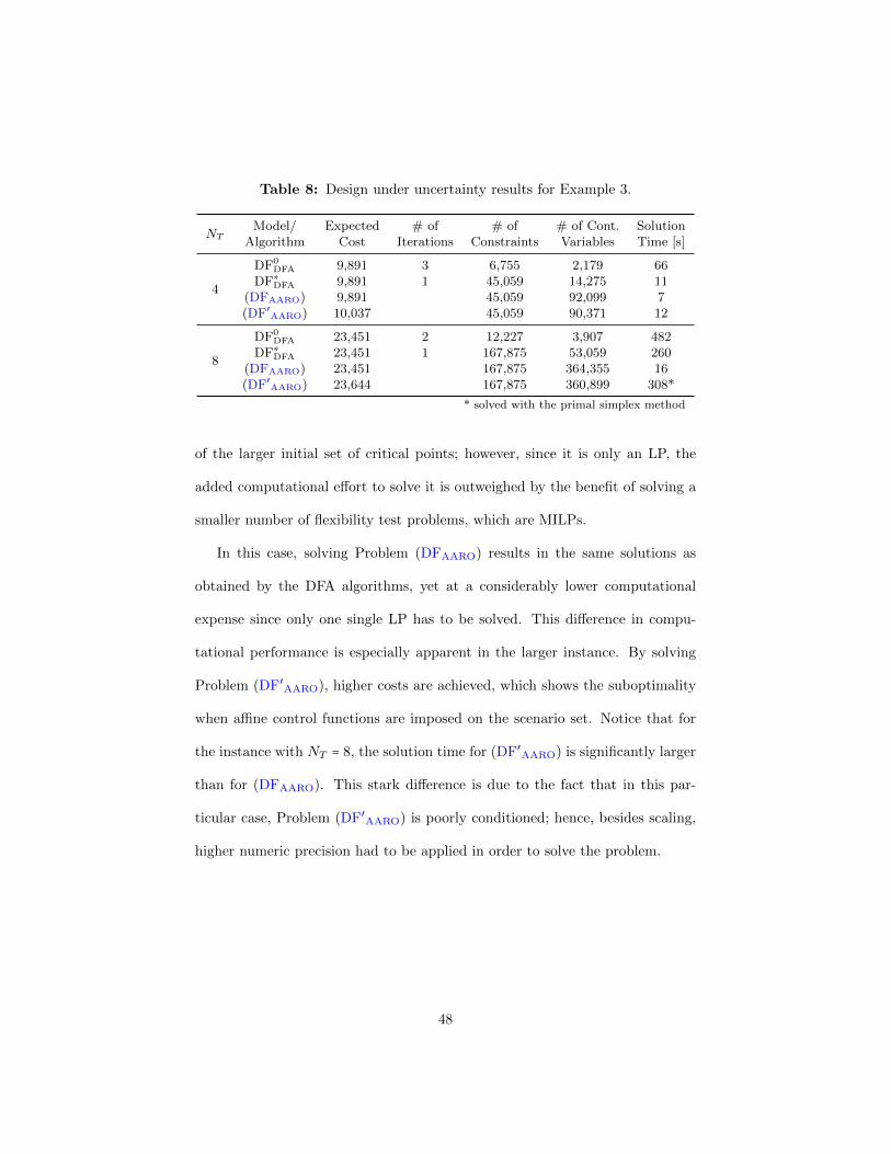
Table 8: Design under uncertainty results for Example 3.

NTModel/ Expected # of # of # of Cont. Solution

Algorithm Cost Iterations Constraints Variables Time [s]

4

DF0DFA 9,891 3 6,755 2,179 66

DF∗DFA 9,891 1 45,059 14,275 11(DFAARO) 9,891 45,059 92,099 7(DF′AARO) 10,037 45,059 90,371 12

8

DF0DFA 23,451 2 12,227 3,907 482

DF∗DFA 23,451 1 167,875 53,059 260(DFAARO) 23,451 167,875 364,355 16(DF′AARO) 23,644 167,875 360,899 308*

* solved with the primal simplex method

of the larger initial set of critical points; however, since it is only an LP, the

added computational effort to solve it is outweighed by the benefit of solving a

smaller number of flexibility test problems, which are MILPs.

In this case, solving Problem (DFAARO) results in the same solutions as

obtained by the DFA algorithms, yet at a considerably lower computational

expense since only one single LP has to be solved. This difference in compu-

tational performance is especially apparent in the larger instance. By solving

Problem (DF′

AARO), higher costs are achieved, which shows the suboptimality

when affine control functions are imposed on the scenario set. Notice that for

the instance with NT = 8, the solution time for (DF′

AARO) is significantly larger

than for (DFAARO). This stark difference is due to the fact that in this par-

ticular case, Problem (DF′

AARO) is poorly conditioned; hence, besides scaling,

higher numeric precision had to be applied in order to solve the problem.

48

Conclusions

In this work, we have examined for linear systems the relationship between

flexibility analysis and robust optimization, which are two approaches to solving

optimization problems under uncertainty that originated from different research

communities (PSE and OR, respectively). Although these two research areas

have been developed independently from each other, they do share some fun-

damental conceptual ideas, such as the use of polyhedral sets to describe the

uncertainty and the worst-case approach to guarantee feasibility for every pos-

sible realization of the uncertainty.

To systematically establish the link between flexibility analysis and robust

optimization, and to compare these different approaches, the three classical

problems from flexibility analysis have been considered: the flexibility test prob-

lem, the flexibility index problem, and design under uncertainty with flexibility

constraints. For LPs with a given general structure, two new solution approaches

have been proposed, where the first derives duality-based reformulations of the

traditional active-set MILP formulations, and the second applies the concept of

affinely adjustable robust optimization (AARO).

The concepts that form the theoretical basis for the three different approaches—

traditional flexibility analysis (TFA), duality-based flexibility analysis (DFA),

and AARO—have been compared. It has become clear that AARO can be seen

as a special case of flexibility analysis, however with a duality-based approach to

solving the problems. It can be shown that in general, AARO is more restrictive

and therefore may be overly conservative. However, it turns out that for LP

models, it is often the case that AARO does predict the same level of flexibility

49

as TFA and DFA.

The three different approaches have been applied to three numerical exam-

ples, verifying some of the theoretical properties of the proposed formulations.

The results further show that DFA and AARO may be computationally more ef-

ficient than TFA. The DFA models exhibit a better computational performance

because of the tightness of the MILP formulations. In the case of AARO, the

main advantage is that only LPs need to be solved; furthermore, no iterative

procedure is required for solving the design under uncertainty problem.

Finally, it should be noted that flexibility analysis is not restricted to models

with inequalities or to linear models since it can be applied to nonlinear models

with equalities. Given the analogies that have been established in this paper

with robust optimization, it would be interesting to examine whether robust

optimization can also be extended to nonlinear models with equalities.

Acknowledgments

The authors gratefully acknowledge the financial support from the National

Science Foundation under Grant No. 1159443.

References

1 Grossmann I, Sargent RWH. Optimum Design of Chemical Plants with Un-

certain Parameters. AIChE Journal. 1978;24(6):1021–1028.

2 Grossmann IE, Calfa BA, Garcia-Herreros P. Evolution of concepts and mod-

els for quantifying resiliency and flexibility of chemical processes. Computers

& Chemical Engineering. 2014;pp. 1–13.

50

3 Friedman Y, Reklaitis GV. Flexible Solutions to Linear Programs under

Uncertainty: Inequality Constraints. AIChE Journal. 1975;21(1):77–83.

4 Friedman Y, Reklaitis GV. Flexible Solutions to Linear Programs under

Uncertainty: Equality Constraints. AIChE Journal. 1975;21(1):83–90.

5 Saboo AK, Morari M, Woodcock DC. Design of resilient processing

plantsVIII. A resilience index for heat exchanger networks. Chemical En-

gineering Science. 1985;40(8):1553–1565.

6 Halemane KP, Grossmann IE. Optimal Process Design Under Uncertainty.

AIChE Journal. 1983;29(3):425–433.

7 Swaney RE, Grossmann IE. An Index for Operational Flexibility in Chemical

Process Design - Part I: Formulation and Theory. AIChE Journal. 1985;

31(4):621–630.

8 Ben-Tal A, El Ghaoui L, Nemirovski A. Robust Optimization. New Jersey:

Princeton University Press. 2009.

9 Bertsimas D, Brown DB, Caramanis C. Theory and Applications of Robust

Optimization. SIAM Review. 2011;53(3):464–501.

10 Gabrel V, Murat C, Thiele A. Recent advances in robust optimization: An

overview. European Journal of Operational Research. 2014;235(3):471–483.

11 Ben-Tal A, Goryashko A, Guslitzer E, Nemirovski A. Adjustable robust

solutions of uncertain linear programs. Mathematical Programming. 2004;

99(2):351–376.

51

12 Kuhn D, Wiesemann W, Georghiou A. Primal and dual linear decision rules

in stochastic and robust optimization. Mathematical Programming. 2011;

130(1):177–209.

13 Birge JR, Louveaux F. Introduction to Stochastic Programming. Springer

Science+Business Media, 2nd ed. 2011.

14 Swaney RE, Grossmann IE. An Index for Operational Flexibility in Chemical

Process Design - Part II: Computational Algorithms. AIChE Journal. 1985;

31(4):631–641.

15 Grossmann IE, Floudas CA. Active constraint strategy for flexibility analysis

in chemical processes. Computers & Chemical Engineering. 1987;11(6):675–

693.

16 Pistikopoulos E, Grossmann I. Optimal retrofit design for improving process

flexibility in nonlinear systems - I. Fixed degree of flexibility. Computers &

Chemical Engineering. 1989;13(9):1003–1016.

17 Pistikopoulos EN, Grossmann IE. Optimal retrofit design for improving pro-

cess flexibility in nonlinear systems - II. Optimal level of flexibility. Computers

& Chemical Engineering. 1989;13(10):1087–1096.

18 Pistikopoulos EN, Mazzuchi TA. A novel flexibility analysis approach for

processes with stochastic parameters. Computers and Chemical Engineering.

1990;14(9):991–1000.

19 Straub DA, Grossmann IE. Integrated Stochastic Metric of Flexibility for

52

Systems with Discrete State and Continuous Parameter Uncertainties. Com-

puters & Chemical Engineering. 1990;14(9):967–985.

20 Dimitriadis VD, Pistikopoulos EN. Flexibility Analysis of Dynamic Systems.

Industrial & Engineering Chemistry Research. 1995;34(12):4451–4462.

21 Rooney WC, Biegler LT. Design for model parameter uncertainty using non-

linear confidence regions. AIChE Journal. 2001;47(8):1794–1804.

22 Rooney WC, Biegler LT. Optimal Process Design with Model Parameter

Uncertainty and Process Variability. AIChE Journal. 2003;49(49):438–449.

23 Ierapetritou MG. New approach for quantifying process feasibility: Convex

and 1-D quasi-convex regions. AIChE Journal. 2001;47(6):1407–1417.

24 Goyal V, Ierapetritou MG. Determination of operability limits using simplicial

approximation. AIChE Journal. 2002;48(12):2902–2909.

25 Goyal V, Ierapetritou MG. Framework for evaluating the feasibil-

ity/operability of nonconvex processes. AIChE Journal. 2003;49(5):1233–

1240.

26 Banerjee I, Ierapetritou MG. Feasibility Evaluation of Nonconvex Systems

Using Shape Reconstruction Techniques. Industrial & Engineering Chemistry

Research. 2005;44:3638–3647.

27 Banerjee I, Pal S, Maiti S. Computationally efficient black-box modeling for

feasibility analysis. Computers & Chemical Engineering. 2010;34(9):1515–

1521.

53

28 Boukouvala F, Ierapetritou MG. Feasibility analysis of black-box processes

using an adaptive sampling Kriging-based method. Computers & Chemical

Engineering. 2012;36:358–368.

29 Soyster AL. Convex Programming with Set-Inclusive Constraints and Ap-

plications to Inexact Linear Programming. Operations Research. 1973;

21(5):1154–1157.

30 Ben-Tal A, Nemirovski A. Robust Convex Optimization. Mathematics of

Operations Research. 1998;23(4):769–805.

31 El Ghaoui L, Oustry F, Lebret H. Robust Solutions to Uncertain Semidefinite

Programs. SIAM Journal on Optimization. 1998;9(1):33–52.

32 Ben-Tal A, Nemirovski A. Robust solutions of uncertain linear programs.

Operations Research Letters. 1999;25(1):1–13.

33 Ben-Tal A, Nemirovski A, Roos C. Robust Solutions of Uncertain Quadratic

and Conic-Quadratic Problems. SIAM Journal on Optimization. 2002;

13(2):535–560.

34 Bertsimas D, Sim M. Robust discrete optimization and network flows. Math-

ematical Programming. 2003;98(1-3):49–71.

35 Ben-Tal A, Nemirovski A. Robust optimization - methodology and applica-

tions. Mathematical Programming. 2002;92(3):453–480.

36 Bertsimas D, Sim M. Tractable approximations to robust conic optimization

problems. Mathematical Programming. 2006;107(1-2):5–36.

54

37 Bertsimas D, Sim M. The Price of Robustness. Operations Research. 2004;

52(1):35–53.

38 Ben-Tal A, Nemirovski A. Robust solutions of Linear Programming prob-

lems contaminated with uncertain data. Mathematical Programming. 2000;

88(3):411–424.

39 Bertsimas D, Pachamanova D, Sim M. Robust linear optimization under

general norms. Operations Research Letters. 2004;32(6):510–516.

40 Chen X, Sim M, Sun P. A Robust Optimization Perspective on Stochastic

Programming. Operations Research. 2007;55(6):1058–1071.

41 Bertsimas D, Goyal V. On the Power of Robust Solutions in Two-Stage

Stochastic and Adaptive Optimization Problems. Mathematics of Operations

Research. 2010;35(2):284–305.

42 Bertsimas D, Litvinov E, Sun XA, Zhao J, Zheng T. Adaptive robust opti-

mization for the security constrained unit commitment problem. IEEE Trans-

actions on Power Systems. 2013;28(1):52–63.

43 Zhao L, Zeng B. Robust unit commitment problem with demand response

and wind energy. IEEE Power and Energy Society General Meeting. 2012;

pp. 1–8.

44 Zeng B, Zhao L. Solving two-stage robust optimization problems using a

column-and-constraint generation method. Operations Research Letters. 2013;

41(5):457–461.

55

45 Bemporad A, Borrelli F, Morari M. Min-Max Control of Constrained Uncer-

tain Discrete-Time Linear Systems. IEEE Transactions on Automatic Con-

trol. 2003;40(9):1234–1236.

46 Chen X, Zhang Y. Uncertain Linear Programs: Extended Affinely Adjustable

Robust Counterparts. Operations Research. 2009;57(6):1469–1482.

47 Bertsimas D, Iancu DA, Parrilo PA. A hierarchy of near-optimal policies for

multistage adaptive optimization. IEEE Transactions on Automatic Control.

2011;56(12):2809–2824.

48 Bertsimas D, Iancu DA, Parrilo PA. Optimality of Affine Policies in Mul-

tistage Robust Optimization. Mathematics of Operations Research. 2010;

35(2):363–394.

49 Bertsimas D, Goyal V. On the power and limitations of affine policies in two-

stage adaptive optimization. Mathematical Programming. 2012;134(2):491–

531.

50 Bertsimas D, Georghiou A. Design of Near Optimal Decision Rules in Mul-

tistage Adaptive Mixed-Integer Optimization. Operations Research. 2015;

63(3):610–627.

51 Postek K, den Hertog D. Multi-Stage Adjustable Robust Mixed-Integer Op-

timization via Iterative Splitting of the Uncertainty Set. CentER Discussion

Paper. 2014;2014-056.

52 Hanasusanto GA, Kuhn D, Wiesemann W, Kuhn D. K-Adaptability in Two-

Stage Robust Binary Programming. Optimization Online. 2015;(July).

56

53 Delage E, Ye Y. Distributionally Robust Optimization Under Moment Un-

certainty with Application to Data-Driven Problems. Operations Research.

2010;58(3):595–612.

54 Goh J, Sim M. Distributionally Robust Optimization and Its Tractable Ap-

proximations. Operations Research. 2010;58(4-part-1):902–917.

55 Lin X, Janak SL, Floudas CA. A new robust optimization approach for

scheduling under uncertainty: I. Bounded uncertainty. Computers & Chemi-

cal Engineering. 2004;28(6-7):1069–1085.

56 Janak SL, Lin X, Floudas CA. A new robust optimization approach for

scheduling under uncertainty: II. Uncertainty with known probability distri-

bution. Computers & Chemical Engineering. 2007;31(3):171–195.

57 Li Z, Ierapetritou MG. Robust optimization for process scheduling under un-

certainty. Industrial and Engineering Chemistry Research. 2008;47(12):4148–

4157.

58 Verderame PM, Floudas CA. Operational Planning of Large-Scale Industrial

Batch Plants under Demand Due Date and Amount Uncertainty. I. Robust

Optimization Framework. Industrial and Engineering Chemistry Research.

2009;48:7214–7231.

59 Mitra S, Grossmann IE, Pinto JM, Arora N. Robust scheduling under time-

sensitive electricity prices for continuous power-intensive processes. In: Pro-

ceedings of the Foundations of Computer-Aided Process Operations 2012.

2012; .

57

60 Vujanic R, Mariethos S, Goulart P, Morari M. Robust Integer Optimization

and Scheduling Problems for Large Electricity Consumers. In: Proceedings of

the 2012 American Control Conference. 2012; pp. 3108–3113.

61 Zhang Q, Grossmann IE, Heuberger CF, Sundaramoorthy A, Pinto JM. Air

Separation with Cryogenic Energy Storage: Optimal Scheduling Considering

Electric Energy and Reserve Markets. AIChE Journal. 2015;61(5):1547–1558.

62 Amaran S, Zhang T, Sahinidis NV, Sharda B, Bury SJ. Medium-term main-

tenance turnaround planning under uncertainty for integrated chemical sites.

Computers & Chemical Engineering. 2016;84:422–433.

63 Zhang Q, Morari MF, Grossmann IE, Sundaramoorthy A, Pinto JM. An

adjustable robust optimization approach to provision of interruptible load by

continuous industrial processes. Submitted for publication. 2015;.

64 Gounaris CE, Wiesemann W, Floudas CA. The Robust Capacitated Vehicle

Routing Problem Under Demand Uncertainty. Operations Research. 2013;

61(3):677–693.

65 Li Z, Ding R, Floudas CA. A Comparative Theoretical and Computational

Study on Robust Counterpart Optimization: I. Robust Linear Optimization

and Robust Mixed Integer Linear Optimization. Industrial & Engineering

Chemistry Research. 2011;50(18):10567–10603.

66 Li Z, Tang Q, Floudas CA. A Comparative Theoretical and Computational

Study on Robust Counterpart Optimization: II. Probabilistic Guarantees on

Constraint Satisfaction. Industrial & Engineering Chemistry Research. 2012;

51(19):6769–6788.

58

67 Du X, Chen W. Towards a better understanding of modeling feasibil-

ity robustness in engineering design. Journal of Mechanical Design. 2000;

122(4):385–394.

68 Yao W, Chen X, Luo W, Van Tooren M, Guo J. Review of uncertainty-

based multidisciplinary design optimization methods for aerospace vehicles.

Progress in Aerospace Sciences. 2011;47(6):450–479.

69 Sundaresan S, Ishii K, Houser DR. A Robust Optimization Procedure With

Variations on Design Variables and Constraints. Engineering Optimization.

1995;24(2):101–117.

70 GAMS Development Corporation. GAMS version 24.4.1. 2015.

71 Sahinidis NV, Grossmann IE, Fornari RE, Chathrathi M. Optimization Model

for Long Range Planning in the Chemical Industry. Computers & Chemical

Engineering. 1989;13(9):1049–1063.

72 Park M, Park S, Mele FD, Grossmann IE. Modeling of Purchase and Sales

Contracts in Supply Chain Optimization. Industrial & Engineering Chemistry

Research. 2006;45:5013–5026.

59