Centralized versus Distributed Manufacturing: A Continuous...

Centralized versus Distributed Manufacturing: A Continuous Location-Allocation Problem

Cristiana Lopes Lara, Ignacio E. Grossmann Department of Chemical Engineering Carnegie Mellon University

EWO Meeting September 30-October 1, 2015

Motivation: Rethinking of traditional manufacturing

2

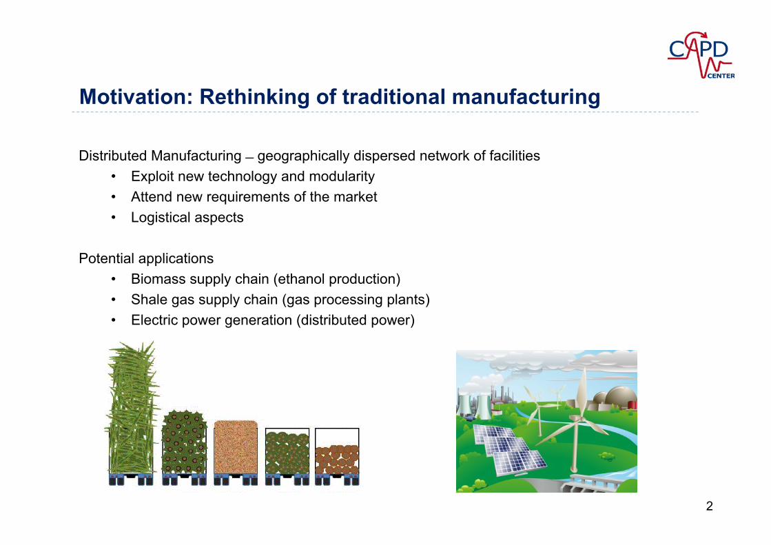
Distributed Manufacturing ̶ geographically dispersed network of facilities •  Exploit new technology and modularity •  Attend new requirements of the market •  Logistical aspects

Potential applications

•  Biomass supply chain (ethanol production)

•  Shale gas supply chain (gas processing plants) •  Electric power generation (distributed power)

3

Motivation: Rethinking of traditional manufacturing

1 J. Brimberg, P. Hansen, N. Mladonovic, and S. Salhi, “A survey of solution methods for the continuous location allocation problem,”, 2008.

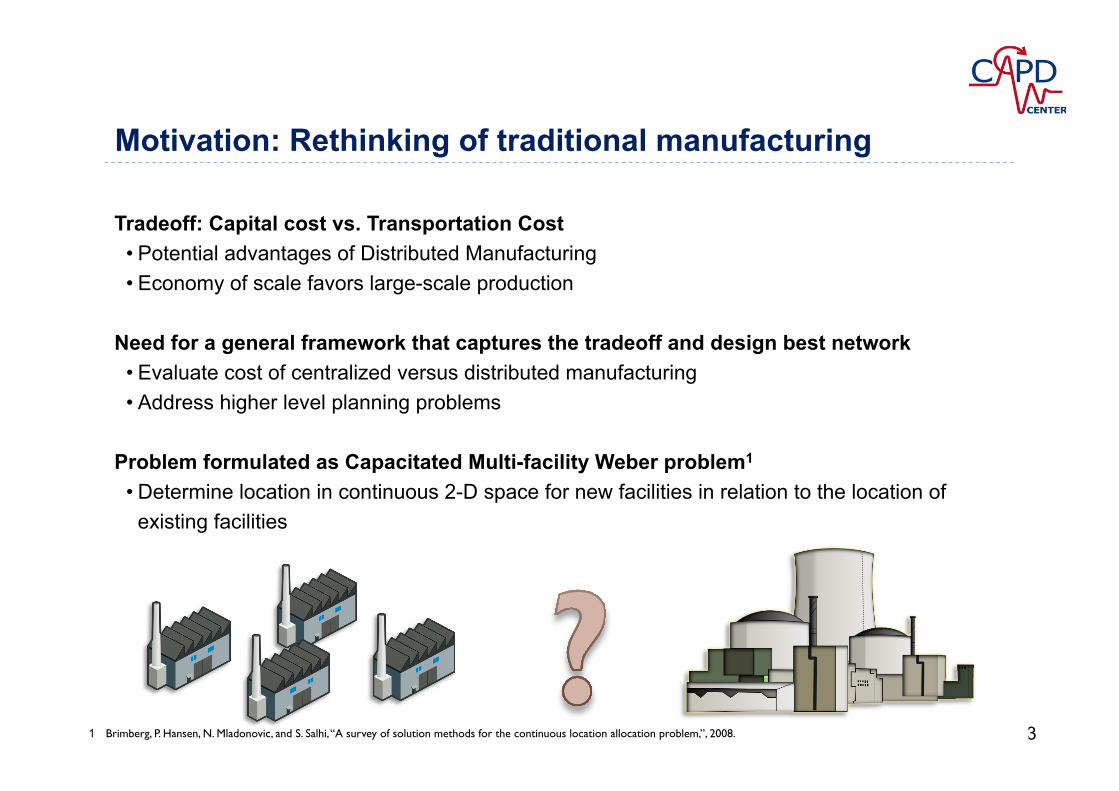
Tradeoff: Capital cost vs. Transportation Cost • Potential advantages of Distributed Manufacturing • Economy of scale favors large-scale production

Need for a general framework that captures the tradeoff and design best network

• Evaluate cost of centralized versus distributed manufacturing • Address higher level planning problems

Problem formulated as Capacitated Multi-facility Weber problem1

• Determine location in continuous 2-D space for new facilities in relation to the location of existing facilities

Background: The Weber Problem

2 A. Weber and C. J. Friedrich, Theory of the Location of Industries, 1929. 3 L. Cooper, “The Transportation-Location Problem,” 1972. 4 H. D. Sherali, I. Al-Loughani, and S. Subramanian, “Global Optimization Procedures for the Capacitated Euclidean and l p Distance Multifacility Location-allocation Problems,” , 2002 5 J. Brimberg, P. Hansen, N. Mladonovic, and S. Salhi, “A survey of solution methods for the continuous location allocation problem,”, 2008.

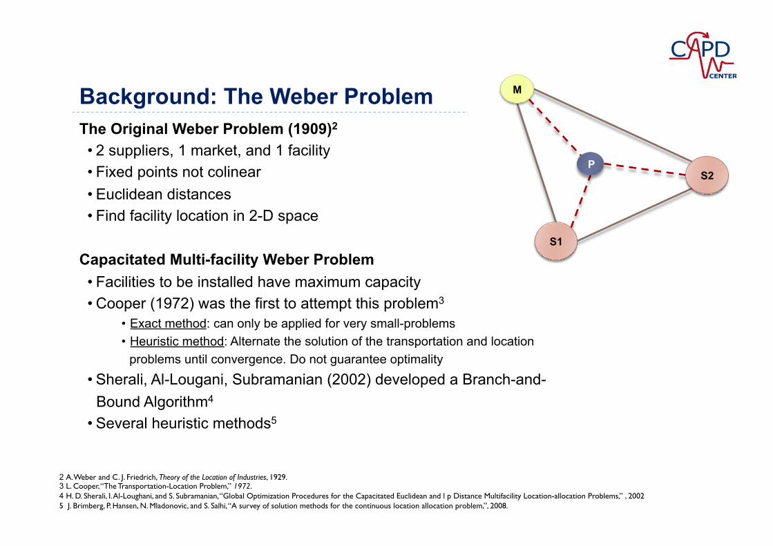
The Original Weber Problem (1909)2

• 2 suppliers, 1 market, and 1 facility • Fixed points not colinear • Euclidean distances • Find facility location in 2-D space

Capacitated Multi-facility Weber Problem • Facilities to be installed have maximum capacity • Cooper (1972) was the first to attempt this problem3

• Exact method: can only be applied for very small-problems • Heuristic method: Alternate the solution of the transportation and location

problems until convergence. Do not guarantee optimality

• Sherali, Al-Lougani, Subramanian (2002) developed a Branch-and-Bound Algorithm4

• Several heuristic methods5

M

PS2

S1

Problem statement

Given: Find:

•  A set of suppliers i, a set of consumer markets j, and their respective fixed location, availability and demand

•  M potential distributed and N potential

centralized set of k single-product facilities, and their corresponding maximum capacity and conversion rate (unknown location)

•  Investment, operating and transportation costs

•  Number, type and 2-D location of facilities to design a manufacturing network that minimizes the cost

f ik, Dik

Zik = {True, False} Zk = {True, False} (xk, yk)

fkj, Dkj

Zkj = {True, False}

5

Continuous variables: xk, yk, fik, fkj, fk, Dik, Dkj Boolean variables: Zk, Zik, Zkj

General Disjunctive Programming (GDP) Formulation

6

Total cost

Choice of facility

Choice of link supplier/facility

Choice of link facility/market

Distance supplier/facility

Distance facility/market

Logic constraints

Availability of raw-material

Mass balances

Market demand

Illustrative example: ethanol production

0

1

2

3

4

5

0 1 2 3 4 5

y (k

m)

x (km)

suppliers i

markets j

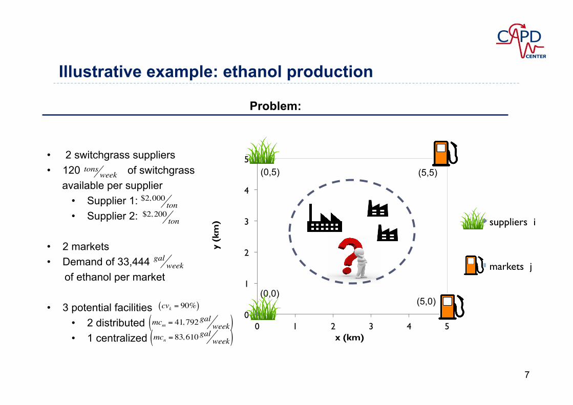
Problem:

•  2 switchgrass suppliers •  120 of switchgrass

available per supplier •  Supplier 1: •  Supplier 2:

•  2 markets •  Demand of 33,444 of ethanol per market •  3 potential facilities

•  2 distributed •  1 centralized

tonsweek

galweek

mcn = 83,610gal

week( )mcm = 41, 792

galweek( )

cvk = 90%( )

$2,000ton

$2,200ton

(0,0)

(0,5)

(5,0)

(5,5)

7


Intuitive answer: 1 centralized facility

0

1

2

3

4

5

0 1 2 3 4 5

y (k

m)

x (km)

suppliers i

markets j

facilities k

(2.5,2.5)

$516,100/week

8


Optimal network: 2 distributed facilities

0

1

2

3

4

5

0 1 2 3 4 5

y (k

m)

x (km)

suppliers i

markets j

facilities k

$503,900/week

(0.5, 0.03)

(0.5, 5.0)

f12=120 ton/week

f21=102.22 ton/week

F12 = 30,767 ton/week

F21 = 33,444 gal/week

9

Illustrative example

6 S. Kolodziej, P. M. Castro, and I. E. Grossmann, “Global optimization of bilinear programs with a multiparametric disaggregation technique,” J, 2013 7 P. M. Castro, “Tightening piecewise McCormick relaxations for bilinear problems,”, 2014. 8 R. Misener, J. P. Thompson, and C. a. Floudas, “Apogee: Global optimization of standard, generalized, and extended pooling problems via linear and logarithmic partitioning schemes,” 2011 .

METHOD Cost . CPU time (s) BARON 503.9 703.2 SCIP 503.9 656.7

Multiparametric Disagreggation6 503.9 1,045.6

Bilevel decomposition 503.9 36.1

Global Optimization:

Computational results

Convex relaxation (lower bound) METHOD Cost . CPU time (s) McCormick 482.4 0.3 Piecewise McCormick7

(16 partitions) 503.8 2065.5

Logarithmic Piecewise McCormick8 (16 partitions) 503.8 35.9

$103week( )

$103week( )

10

Bilevel decomposition: Background

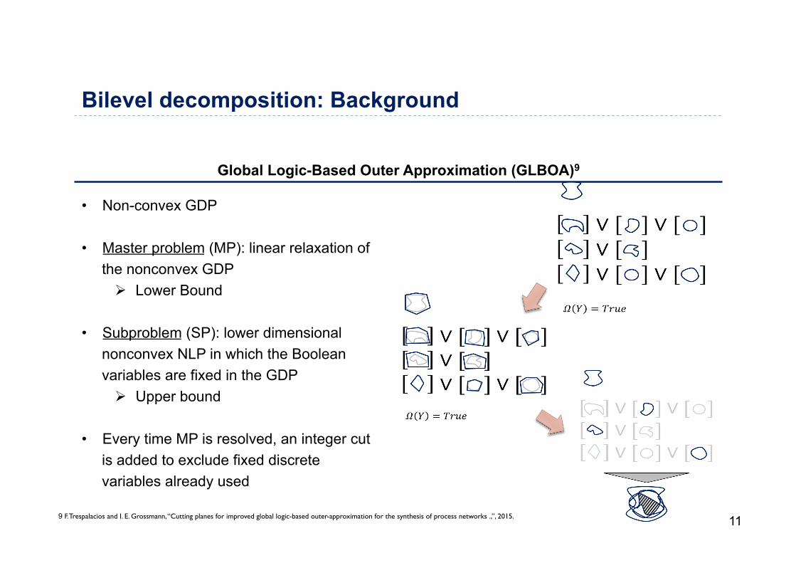
Global Logic-Based Outer Approximation (GLBOA)9

•  Non-convex GDP

•  Master problem (MP): linear relaxation of the nonconvex GDP Ø  Lower Bound

•  Subproblem (SP): lower dimensional

nonconvex NLP in which the Boolean variables are fixed in the GDP Ø  Upper bound

•  Every time MP is resolved, an integer cut is added to exclude fixed discrete variables already used

9 F. Trespalacios and I. E. Grossmann, “Cutting planes for improved global logic-based outer-approximation for the synthesis of process networks .,”, 2015. 11

Bilevel decomposition algorithm

Algorithm Description

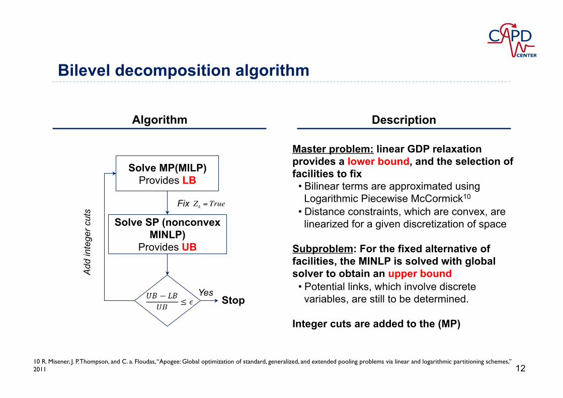
Solve MP(MILP) Provides LB

Add

inte

ger c

uts

Master problem: linear GDP relaxation provides a lower bound, and the selection of facilities to fix

• Bilinear terms are approximated using Logarithmic Piecewise McCormick10

• Distance constraints, which are convex, are linearized for a given discretization of space

Subproblem: For the fixed alternative of facilities, the MINLP is solved with global solver to obtain an upper bound

• Potential links, which involve discrete variables, are still to be determined.

Integer cuts are added to the (MP)

Stop Yes

Solve SP (nonconvex MINLP)

Provides UB

Fix Zk = True

10 R. Misener, J. P. Thompson, and C. a. Floudas, “Apogee: Global optimization of standard, generalized, and extended pooling problems via linear and logarithmic partitioning schemes,” 2011 12

Large-scale problems: Example 1

Problem

0

5

10

15

20

25

30

0 5 10 15 20 25 30

y (k

m)

x (km)

suppliers i

markets j

•  10 suppliers •  120 of raw

material available per supplier

•  10 markets •  Demand of 100 per market

•  12 potential facilities •  10 distributed •  2 centralized

tonsweek

tonsweek

mcn =1000 tons week( )mcm =100 tons week( )cvk = 90%( )

13


Optimal network found: 10 distributed facilities

$28,991,000 /week

14

0

5

10

15

20

25

30

0 5 10 15 20 25 30

y (k

m)

x (km)

f7 = 100

f4 = 100

f5 = 100

f8 = 100

f1 = 100

f10 = 100 f2 = 100

f6 = 100

f3 = 100

f9 = 100

supplier i market j facilities k


* Exceeded maximum CPU time ** Estimated gap For the Bilevel Decomposition Algorithm, the master problem (MILP) was solved using CPLEX and the subproblem (nonconvex MINLP) was solved using BARON

METHOD Cost Optimality gap (%) CPU time (hrs)

BARON 29,054 21% 12*

SCIP 29,892 92% 12*

Bilevel Decomposition 28,991 9%** 4*


$103week( )


15


0

5

10

15

20

25

30

0 5 10 15 20 25 30

y (

km)

x (km)

suppliers i

markets j

Problem

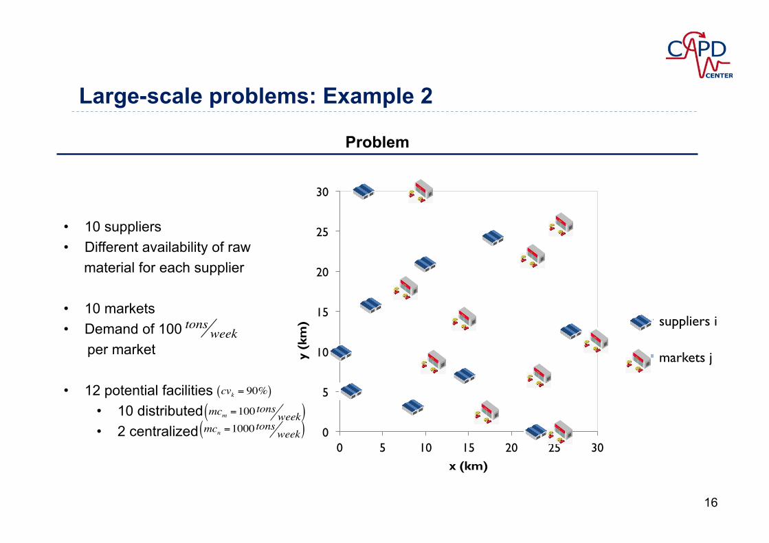
•  10 suppliers •  Different availability of raw

material for each supplier •  10 markets •  Demand of 100 per market

•  12 potential facilities •  10 distributed •  2 centralized

tonsweek

mcn =1000 tons week( )mcm =100 tons week( )cvk = 90%( )

16


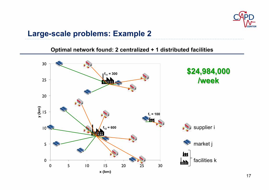
Optimal network found: 2 centralized + 1 distributed facilities

0

5

10

15

20

25

30

0 5 10 15 20 25 30

y (k

m)

x (km)

$24,984,000 /week

17

f1 = 100

f12 = 600

f11 = 300

supplier i market j facilities k

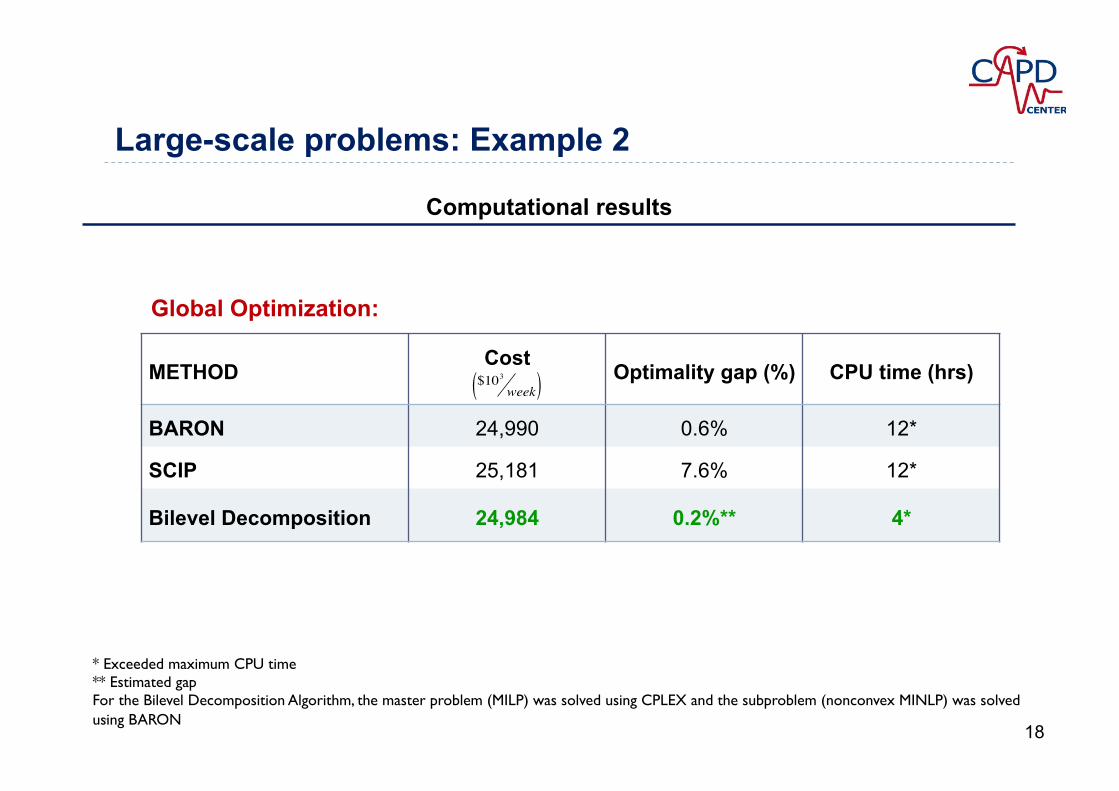
METHOD Cost Optimality gap (%) CPU time (hrs)

BARON 24,990 0.6% 12*

SCIP 25,181 7.6% 12*

Bilevel Decomposition 24,984 0.2%** 4*


* Exceeded maximum CPU time ** Estimated gap For the Bilevel Decomposition Algorithm, the master problem (MILP) was solved using CPLEX and the subproblem (nonconvex MINLP) was solved using BARON

$103week( )



18

Conclusions

Nonconvex GDP reformulated as an MINLP Commercial global solvers can solve small problems fairly easy Computationally expensive to solve large-scale problems

•  Bilevel decomposition algorithm o  Although at this point it cannot rigorously solve the large-scale problems to

optimality, provides superior results o  Potential to be improved

19

Future work

Develop new cuts to tighten the relaxation • Improve the performance of both the solvers and the algorithm

Rethink master problem formulation • So as it can be solved to optimality faster

Apply formulation to different problem structures • Investigate how the network configuration is affected by changes in the parameters • Explore which conditions favor distributed and/or centralized manufacturing networks.

Apply the model to biomass and electric power systems supply chain

20

Centralized versus Distributed Manufacturing: A Continuous...

Documents

Transcript of Centralized versus Distributed Manufacturing: A Continuous...