Advances in Mathematical Programming...
58
Advances in Mathematical Programming Models Advances in Mathematical Programming Models for Enterprise-wide Optimization Ignacio E. Grossmann Center for Advanced Process Decision-making Department of Chemical Engineering Department of Chemical Engineering Carnegie Mellon University Pittsburgh, PA 15213, U.S.A. EWO Seminar April 24, 2012
Transcript of Advances in Mathematical Programming...

Advances in Mathematical Programming ModelsAdvances in Mathematical Programming Models for Enterprise-wide Optimization
Ignacio E. GrossmannCenter for Advanced Process Decision-making
Department of Chemical EngineeringDepartment of Chemical EngineeringCarnegie Mellon UniversityPittsburgh, PA 15213, U.S.A.
EWO SeminarApril 24, 2012

Motivation for Enterprise-wide Optimization
US chemical industry:19 % of the world’s chemical output
Facing stronger international competition
US$689 billion revenues10% of US exports
Facing stronger international competitionPressure for reducing costs, inventories and ecological footprint
Major goal: Enterprise-wide Optimization
Recent research area in Process Systems Engineering:
Recent research area in Process Systems Engineering: Grossmann (2005); Varma, Reklaitis, Blau, Pekny (2007)
A major challenge: optimization models and solution methodsj g p

Enterprise-wide Optimization (EWO)
EWO involves optimizing the operations of R&D,material supply, manufacturing, distribution of a company to reduce costs, inventories, ecological footprint and to maximize profits, responsiveness .
Key element: Supply Chain
Example: petroleum industry
WellheadWellhead PumpPumpTradingTrading Transfer of Crude
Transfer of Crude
Refinery Processing
Refinery Processing
Schedule ProductsSchedule Products
Transfer of Products
Transfer of Products
TerminalLoadingTerminalLoading
3

I I t ti f l i h d li d t l
Key issues:I. Integration of planning, scheduling and control
Planning Economicsmonths, years Multiple Planning
Scheduling
Economics
Feasibility Delivery
days, weeks
ptime scales
Control
Delivery
Dynamic Performance
secs, mins
Planning LP/MILPMultiple models
Scheduling MI(N)LP
RTO MPC
4
Control RTO, MPC

II. Integration of information and models/solution methods
Strategic OptimizationModeling System
Tactical Optimization
Analytical Analytical ITIT
Strategic AnalysisStrategic Analysis
LongLong--Term Tactical Term Tactical
ScopeScope
Tactical OptimizationModeling System
Production Planning OptimizationModeling Systems
Logistics OptimizationLogistics OptimizationModeling SystemModeling System
Demand Demand Forecasting and OrderForecasting and OrderManagement SystemManagement System
o go g e act cae act caAnalysisAnalysis
ShortShort--Term Tactical Term Tactical AnalysisAnalysis
Production Scheduling Optimization Modeling Systems
Distributions Scheduling Optimization Distributions Scheduling Optimization Modeling SystemsModeling Systems
Operational Operational AnalysisAnalysis
Materials RequirementMaterials RequirementPlanning SystemsPlanning Systems
Distributions RequirementsDistributions RequirementsPlanning SystemPlanning System
Transactional ITTransactional IT
Enterprise ResourceEnterprise ResourcePlanning SystemPlanning System
E l DE l D
5Source: Tayur, et al. [1999]Source: Tayur, et al. [1999]
External DataExternal DataManagement SystemsManagement Systems

Optimization Modeling Framework:Mathematical Programmingg g
fZ )(i Obj i f i
yx htsyxfZ
0),(..),(min
Objective function
Constraints
mnRyxg
100, )(
Constraints
mn yRx 1,0,
MINLP: Mixed-integer Nonlinear Programming Problem
6

fZ )(i
Linear/Nonlinear Programming (LP/NLP)
xgx hts
xfZ
0)(0)( ..
)(min
nRxxg
0)(
LP Codes: Very large-scale models LP Codes:CPLEX, XPRESS, GUROBI, XA
NLP C d
y gInterior-point: solvable polynomial time
NLP Codes:CONOPT Drud (1998)IPOPT Waechter & Biegler (2006)Knitro Byrd, Nocedal, Waltz (2006)
Large-scale modelsRTO: Marlin, Hrymak (1996)Zavala, Biegler (2009)Knitro Byrd, Nocedal, Waltz (2006)
MINOS Murtagh, Saunders (1995)SNOPT Gill, Murray, Saunders(2006)BARON Sahinidis et al. (1998)C B l i M (2008)
Global
Issues:ConvergenceNonconvexities
77
Couenne Belotti, Margot (2008) Optimization
yxfZ ),(min Mixed-integer Linear/Nonlinear Programming (MILP/MINLP)
yxgyx hts
0,0),(..)(
mn yRx 1,0,
MILP Codes:Great Progress over last decade despite NP-hardPlanning/Scheduling: Lin, Floudas (2004)
CPLEX, XPRESS, GUROBI, XA
MINLP Codes:
g g , ( )Mendez, Cerdá , Grossmann, Harjunkoski (2006)Pochet, Wolsey (2006)
MINLP Codes:DICOPT (GAMS) Duran and Grossmann (1986)a-ECP Westerlund and Petersson (1996)MINOPT Schweiger and Floudas (1998)MINLP BB (AMPL)Fl h d L ff (1999)
New codes over last decadeLeveraging progress in MILP/NLP
MINLP-BB (AMPL)Fletcher and Leyffer (1999)SBB (GAMS) Bussieck (2000)Bonmin (COIN-OR) Bonami et al (2006)FilMINT Linderoth and Leyffer (2006)
Issues:ConvergenceNonconvexitiesScalability
88
yff ( )BARON Sahinidis et al. (1998)Couenne Belotti, Margot (2008)
GlobalOptimization
Scalability

Modeling systems g yMathematical Programming
GAMS (Meeraus et al, 1997)
AMPL (Fourer et al., 1995)
AIMSS (Bisschop et al. 2000)
1 Al b i d li t ti d l1. Algebraic modeling systems => pure equation models
2. Indexing capability => large-scale problems
3. Automatic differentiation => no derivatives by user3. Automatic differentiation no derivatives by user
4. Automatic interface with LP/MILP/NLP/MINLP solvers
Constraint Programming OPL (ILOG), CHIP (Cosytech), Eclipse Have greatly facilitatedHave greatly facilitated development and
implementation of Math Programming models
99

min kZ c f (x ) Generalized Disjunctive Programming (GDP)
min
0
kk
jk
Z c f (x )
s.t. r(x )
Y
Disjunctions
Raman, Grossmann (1994)
0jk
jkk
k jk
g (x ) k K j J
c γ
Disjunctions
1nk
jk
Ω Y true
x R , c RY true false
Boolean Variables
Logic Propositions
Continuous Variables jkY true, false Boolean Variables
Codes:LOGMIP (GAMS-Vecchietti, Grossmann, 2005)EMP (GAMS F i M 2010)EMP (GAMS-Ferris, Meeraus, 2010)
Other logic-based: Constraint Programming (Hooker, 2000)Codes: CHIP Eclipse ILOG-CP
1010
Codes: CHIP, Eclipse, ILOG CP
Optimization Under Uncertainty
Multistage Stochastic Programming
min )]...]()([...)()([ 222112
NNN xcExcExcz N
Multistage Stochastic ProgrammingBirge & Louveaux, 1997; Sahinidis, 2004
s.t. 111 hxW )()()( 222211 hxWxT
)()()()( 111 NNNNNNN hxWxT
…
Exogeneous uncertainties(e.g. demands)
1,...,2,0)(,01 Ntxx tt
Special case: two-stage programming (N=2)
Planning with endogenous uncertainties (e g yields size resevoir test drug):
x1 stage 1 x2 recourse (stage 2)
11
Planning with endogenous uncertainties (e.g. yields, size resevoir, test drug):Goel, Grossmann (2006), Colvin, Maravelias (2009), Gupta, Grossmann (2011)

Robust Optimization
Ben-Tal et al., 2009; Bertsimas and Sim (2003)
Major concern: feasibility over uncertainty set
Robust scheduling: gLin, Janak, Floudas (2004); Li, Ierapetritou (2008)
12

Multiobjective Optimization
yxf ),(1
Pareto optimalyxfZ
.......),(min 2
f2
Pareto-optimalsolutions
yxgyx hts
0),(0),( ..
f1mn yRx 1,0,
-constraint method: Ehrgott (2000)
Parametric programming: Pistikopoulos, Georgiadis and Dua (2007)
13

Decomposition TechniquesLagrangean decompositionGeoffrion (1972) Guinard (2003)
Benders decomposition
Benders (1962), Magnanti, Wing (1984)
A
Complicating Constraints
x1 x2 x3
Complicating Variables
x1 x2 x3yA
D1
D2
D1
D
D2A
D3
2
max Tc xli i
D3
T T
1,.. 1 0
i i i
st Ax bD x d i nx X x x i n x
complicatingconstraints 1,..
max
1,..0, 0, 1,..
T Ti i
i n
i i i
i
a y c x
st Ay D x d i ny x i n
complicatingvariables
1414
, 1,.. , 0i ix X x x i n x i
Widely used in EWO Applied in 2-stage Stochastic Programming
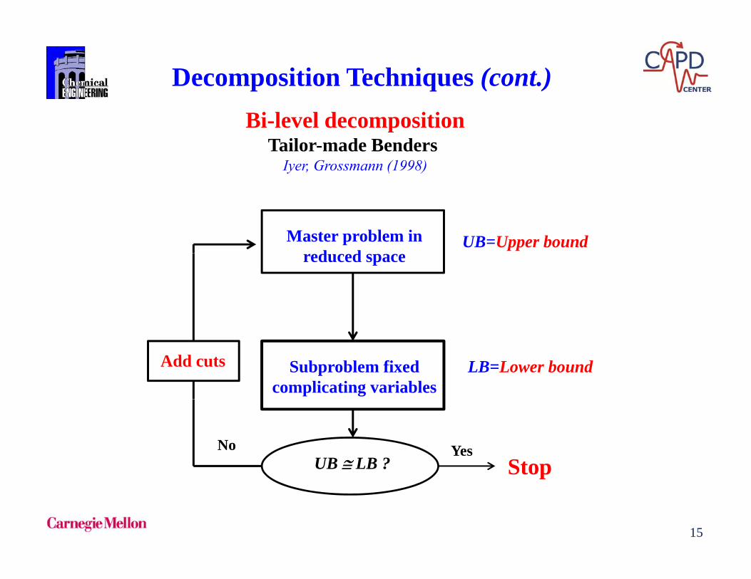
Decomposition Techniques (cont.)Bi-level decomposition
Tailor-made Benders Iyer, Grossmann (1998)
Master problem ind d
UB=Upper boundreduced space
Subproblem fixedcomplicating variables
LB=Lower boundAdd cuts
UB LB ?Yes
StopNo
15
Stop

PITA ProjectSpecial industrial interest group in CAPD:“Enterprise-wide Optimization for Process Industries”
Multidisciplinary team:Chemical engineers Operations Research Industrial Engineering
http://egon.cheme.cmu.edu/ewocp/
Researchers:Carnegie Mellon: Ignacio Grossmann (ChE)
L Bi l (ChE)
Chemical engineers, Operations Research, Industrial Engineering
Larry Biegler (ChE)Nicola Secomandi (OR)John Hooker (OR)
L hi h U i it K t S h i b (I d E )Lehigh University: Katya Scheinberg (Ind. Eng)Larry Snyder (Ind. Eng.)Jeff Linderoth (Ind. Eng.)
16

Projects and case studies with partner companies:“Enterprise-wide Optimization for Process Industries”
ABB: Optimal Design of Supply Chain for Electric MotorsABB: Optimal Design of Supply Chain for Electric Motors Contact: Iiro Harjunkoski Ignacio Grossmann, Analia Rodriguez
Air Liquide: Optimal Coordination of Production and Distribution of Industrial GasesContact: Jean Andre, Jeffrey Arbogast Ignacio Grossmann, Vijay Gupta, Pablo Marchetti
Air Products: Design of Resilient Supply Chain Networks for Chemicals and GasesContact: James Hutton Larry Snyder, Katya Scheinbergy y , y g
Braskem: Optimal production and scheduling of polymer productionContact: Rita Majewski, Wiley Bucey Ignacio Grossmann, Pablo Marchetti
Cognizant: Optimization of gas pipelinesContact: Phani Sistu Larry Biegler, Ajit Gopalakrishnan
Dow: Multisite Planning and Scheduling Multiproduct Batch Processes Contact: John Wassick Ignacio Grossmann, Bruno Calfa
Dow: Batch Scheduling and Dynamic Optimization Contact: John Wassick Larry Biegler, Yisu Nie
Ecopetrol: Nonlinear programming for refinery optimizationContact: Sandra Milena Montagut Larry Biegler, Yi-dong Lang
ExxonMobil: Global optimization of multiperiod blending networksExxonMobil: Global optimization of multiperiod blending networksContact: Shiva Kameswaran, Kevin Furman Ignacio Grossmann, Scott Kolodziej
ExxonMobil: Design and planning of oil and gasfields with fiscal constraintsContact: Bora Tarhan Ignacio Grossmann, Vijay Gupta
G&S Construction: Modeling & Optimization of Advanced Power PlantsContact: Daeho Ko and Dongha Lim Larry Biegler, Yi-dong Lang
Praxair: Capacity Planning of Power Intensive Networks with Changing Electricity PricesContact: Jose Pinto Ignacio Grossmann, Sumit Mitra
UNILEVER: Scheduling of ice cream productionContact: Peter Bongers Ignacio Grossmann, Martijn van Elzakker
BP*: Refinery Planning with Process ModelsContact: Ignasi Palou-Rivera Ignacio Grossmann, Abdul Alattas
17
Contact: Ignasi Palou Rivera Ignacio Grossmann, Abdul AlattasPPG*: Planning and Scheduling for Glass Production
Contact: Jiao Yu Ignacio Grossmann, Ricardo LimaTOTAL*: Scheduling of crude oil operations
Contact: Pierre Pestiaux Ignacio Grossmann, Sylvain Mouret

Major Issues
-Linear vs Nonlinear models
- The multi-scale optimization challenge
- The uncertainty challenge
E i f
- Computational efficiency in large-scale problems
- Economics vs performance
- Commercial vs. Off-the Shelf Software
Computational efficiency in large scale problems
18

Why Emphasis on Linear?Rich developments in Batch Scheduling dominated by MILP
(A) Time Domain Representation- Discrete time- Continuous time
TIME
TASK
TIME
TASK
p g y
(B) Event RepresentationDiscrete Time
- Global time intervalsContinuous Time
- Time slots Unit-specific direct precedence Global direct or general precedence
TIME
EVENTS
TIME
TASK
- Time slots, Unit-specific direct precedence, Global direct or general precedence,Global time points Unit- specific time event
(C) Plant topology- Multistage
Network (STN RTN)
7
4321
8
1110
21
20
24
23
- Network (STN,RTN)
65
98
1918 2
2 25
24
(D) Objective Functions: Makespan, Earliness/ Tardiness, Profit, Inventory, Cost
Most cited paper: Kondili, Pantelides, Sargent (1993) MILP-STN Paper: 460 citations (Web Science)Pioneers: Reklaitis, Rippin: late 1970’s
1919
Reviews: Lin, Floudas (2004), Mendez, Cerdá , Grossmann, Harjunkoski (2006)
Unification and Generalization: Sundaramoorthy, Maravelias (2011)
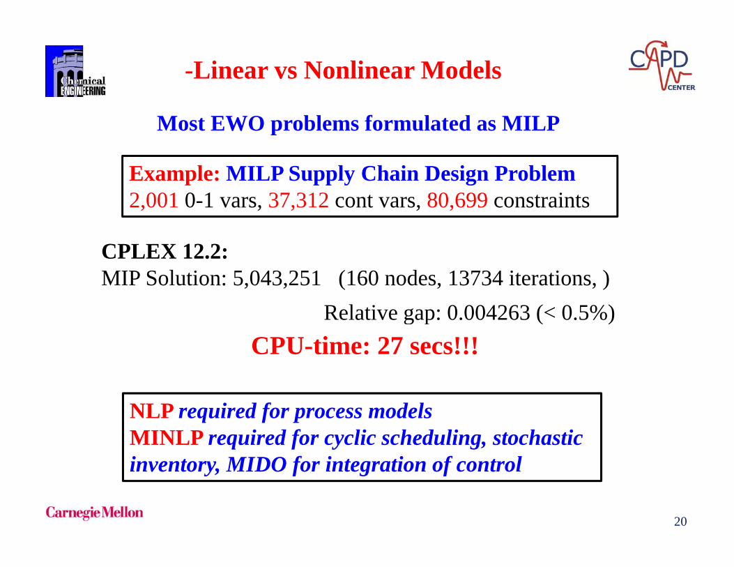
-Linear vs Nonlinear Models
Example: MILP Supply Chain Design Problem
Most EWO problems formulated as MILP
Example: MILP Supply Chain Design Problem2,001 0-1 vars, 37,312 cont vars, 80,699 constraints
CPLEX 12 2CPLEX 12.2: MIP Solution: 5,043,251 (160 nodes, 13734 iterations, )
Relative gap: 0.004263 (< 0.5%)Relative gap: 0.004263 ( 0.5%)CPU-time: 27 secs!!!
NLP required for process modelsMINLP required for cyclic scheduling, stochastic inventory MIDO for integration of control
20
inventory, MIDO for integration of control

Nonlinear CDU Models in Refinery Planning Optimization
Typical Refinery Configuration (Adapted from Aronofsky, 1978)
Alattas, Palou-Rivera, Grossmann (2010)
butaneFuel gas
Prem.SR Fuel gas
Cat Ref
Crude1,…
Gasoline
Reg.Gasoline
SR Naphtha
SR Gasoline
Distillateblending
CDUDistillate
SR DistillateProduct Blending
blending
Gas oil
Cat Crack
Crude2,…. Fuel Oil
SR GO
Hydrotreatment
blending
Treated Residuum
SR Residuum
21
1000
1200
Li
He
Res
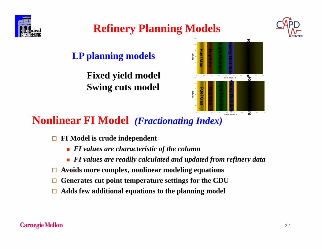
Refinery Planning Models
LP planning models
Fixed yield model 1200
R0
200
400
600
800
0% 10% 20% 30% 40% 50% 60% 70% 80% 90%
C d V l %
TBP
(ºF)
Fuel Gas
Naphtha
ight Distillate
eavy Distillate
siduum B
ottomFixed yield modelSwing cuts model
200
400
600
800
1000
1200
TBP
(ºF)
Fuel Gas
Naphtha
Light Distillat
Heavy D
istillat
Residuum
Botto
Crude Volume %
Nonlinear FI Model (Fractionating Index)
FI Model is crude independent
00% 10% 20% 30% 40% 50% 60% 70% 80% 90%
Crude Volume %
e te om
FI Model is crude independent FI values are characteristic of the column FI values are readily calculated and updated from refinery data
Avoids more complex, nonlinear modeling equations Avoids more complex, nonlinear modeling equations Generates cut point temperature settings for the CDU Adds few additional equations to the planning model
22

Planning Model Example Results
Crude1 Louisiana Sweet Lightest
Crude2 Texas Sweet
Crude3 Louisiana Sour
Comparison of nonlinear fractionation index (FI) with the
Crude3 Louisiana Sour
Crude4 Texas Sour Heaviest
p f ( )fixed yield (FY) and swing cut (SC) models
Economics: maximum profit
Model Case1 Case2 Case3
FI yields highest profit
FI 245 249 247
SC 195 195 191
FY 51 62 59
23

Model statistics LP vs NLP FI model larger number of equations and variables Impact on solution time ~30% nonlinear variables
Model Variables EquationsNonlinear Variables
CPU Time Solver
2 CrudeOil Case
FY 128 143 0.141 CPLEXSC 138 163 0.188FI 1202 1225 348 0.328 CONOPT
3 Crude FY 159 185 0.250 CPLEXSC 174 215 0 281Oil Case SC 174 215 0.281FI 1770 1808 522 0.439 CONOPT
4 CrudeOil Case
FY 192 231 0.218 CPLEXSC 212 271 0.241FI 2340 2395 696 0.860 CONOPT
24

- Solution large-scale problems:
Strategy 1: Exploit problem structure (TSP)
Strategy 2: DecompositionStrategy 2: Decomposition
Strategy 3: Heuristic methods to obtain “good feasible solutions”
25

Design Supply Chain Stochastic InventoryYou, Grossmann (2008), ( )
• Major Decisions (Network + Inventory)k b f C d h i l i i b Network: number of DCs and their locations, assignments between
retailers and DCs (single sourcing), shipping amounts Inventory: number of replenishment, reorder point, order quantity,
safety stock
• Objective: (Minimize Cost)
Total cost = DC installation cost + transportation cost + fixed order cost+ working inventory cost + safety stock cost+ working inventory cost + safety stock cost
26Trade-off: Transportation vs inventory costs

supplierDC i ll i
INLP Model Formulation
retailersupplier
DC
DC – retailer transportation
DC installation cost
EOQ
Safety StockXj Yij
Assignm
Supplier RetailersDistribution Centers
ments
N INLP27
Nonconvex INLP: 1. Variables Yij can be relaxed as continuous2. Problem reformulated as MINLP3. Solved by Lagrangean Decomposition (by distribution centers)
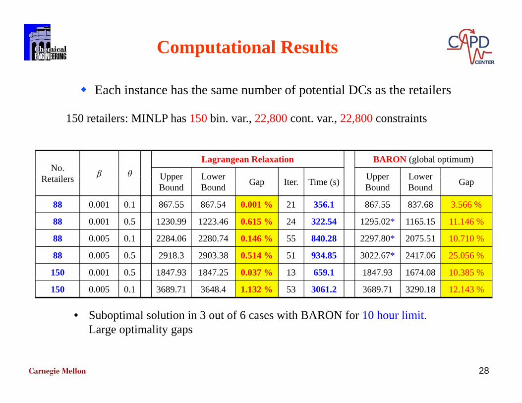
Computational Results
Each instance has the same number of potential DCs as the retailers
150 retailers: MINLP has 150 bin. var., 22,800 cont. var., 22,800 constraints
No. R il β θ
Lagrangean Relaxation BARON (global optimum)
Upper Lower Upper LowerRetailers β θ Upper Bound
Lower Bound Gap Iter. Time (s) Upper
BoundLower Bound Gap
88 0.001 0.1 867.55 867.54 0.001 % 21 356.1 867.55 837.68 3.566 %
88 0.001 0.5 1230.99 1223.46 0.615 % 24 322.54 1295.02* 1165.15 11.146 %
88 0.005 0.1 2284.06 2280.74 0.146 % 55 840.28 2297.80* 2075.51 10.710 %
88 0.005 0.5 2918.3 2903.38 0.514 % 51 934.85 3022.67* 2417.06 25.056 %
150 0.001 0.5 1847.93 1847.25 0.037 % 13 659.1 1847.93 1674.08 10.385 %
150 0.005 0.1 3689.71 3648.4 1.132 % 53 3061.2 3689.71 3290.18 12.143 %
• Suboptimal solution in 3 out of 6 cases with BARON for 10 hour limit.Large optimality gaps
28
Large optimality gaps

The multi-scale optimization challenge
Temporal integration long-term, medium-term and p g g ,short-term Bassett, Pekny, Reklaitis (1993), Gupta, Maranas (1999), Jackson, Grossmann (2003), Stefansson, Shah, Jenssen (2006), Erdirik-Dogan, Grossmann (2006), Maravelias, Sung (2009), Li and Ierapetritou (2009), Verderame , Floudas (2010)
Spatial integration geographically distributed sites G t M (2000) T i ki Sh h P t lid (2001)Gupta, Maranas (2000), Tsiakis, Shah, Pantelides (2001), Jackson, Grossmann (2003), Terrazas, Trotter, Grossmann (2011)
Decomposition is key: Benders, Lagrangean, bilevel
29

Multi-site planning and scheduling involves differenttemporal and spatial scales Terrazas, Grossmann (2011)
Planning1 Week 1 Week 2 Week t
Weekly aggregate production:• Amounts• Aggregate sequencing
d l
Scheduling
Site
hr
model(TSP constraints)
Detailed operation• Start and end times
Week 1 Week 2 Week t• Allocation to parallel
lines
Different Temporal Scales
Different Spati
Planning
pial Scales
Weekly aggregate production:
Scheduling
Site
s Week 1 Week 2 Week t
hr Detailed operation
3030
Schedulinghr
Week 1 Week 2 Week t
Detailed operation

Bilevel decomposition + Lagrangean decomposition
Market 1ths ˆ
sht • Bilevel decomposition
Market 2Production
Site 1
Production Site n-1
po Decouples planning from
schedulingo Integrates across temporal
scale Market 3
Production Site 2 Production
Site n• Lagrangean decomposition
o Decouples the solution of each production site
Shipments ( sht) leaving production sites
Shipments ( sht) arriving at marketsths ˆ
sht
each production siteo Integrates across spatial
scale
3131

Example: 3 sites, 3 products, 3 months
B C BSite 1 A
Profit: $ 2.576 million
Site 2 A
B
Month 1 Month 2
Site 3
Month 3
A A
Site 1 Market 1
Market 2
Site 3
3232
Site 2Market3

Large-scale problems
Full spaceBi-levelBi level + LagrangeanBi-level + Lagrangean
3333
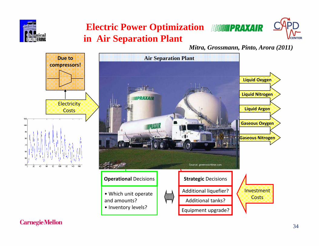
Electric Power Optimizationin Air Separation Plant
Mi G Pi A (2011)Air Separation PlantDue to
compressors!
Mitra, Grossmann, Pinto, Arora (2011)
Liquid Oxygen
Electricity
Liquid Nitrogen
Li id ACosts Liquid Argon
Gaseous Oxygen
Gaseous NitrogenGaseous Nitrogen
InvestmentCosts
Additional liquefier?
Strategic Decisions
Additional tanks?• Which unit operateand amounts?
Operational Decisions
34
Additional tanks?
Equipment upgrade?
and amounts?• Inventory levels?

Multiscale design approachSeasonal variations with cyclic weeks
Year 1, spring: Investment decisions
Year 2, spring: Investment decisions
Year 1, summer: Investment decisions
Year 1, fall: Investment decisions
Year 1, winter: Investment decisions
150.00
200.00
250.00
Spring
150.00
200.00
250.00
Summer
150.00
200.00
250.00
Fall
150.00
200.00
250.00
Winter
Mo Tu We Th Fr Sa Su Mo Tu Su… Mo Tu Su… Mo Tu Su… …
0.00
50.00
100.00
1 25 49 73 97 121 145 0.00
50.00
100.00
1 25 49 73 97 121 145 0.00
50.00
100.00
1 25 49 73 97 121 145 0.00
50.00
100.00
1 25 49 73 97 121 145
• Horizon: 5-15 years, each year has 4 periods (spring, summer, fall, winter)
• Each period is represented by one week on an hourly basisV i i t l t i it i d d d t fi ti l t
Spring Summer Fall Winter
Varying inputs: electricity prices, demand data, configuration slates
• Each representative week is repeated in a cyclic manner (For each season: 13 weeks reduced to 1 week) => 672 hrs vs 8736 hrs
• Connection between periods: Only through investment (design) decisions
• Design decisions are modeled by discrete equipment sizes => MILP
3535

Retrofit air separation plant: selection and timing of design alternatives are degrees of freedom
Air Separation PlantSuperstructureLIN
1.TankLIN
2.Tank?
LAR1 Tank
LAR2 Tank?
Liquid Nitrogen
Liquid Argon
Existing equipment
p
LOX1.Tank
LOX2.Tank?
1.Tank 2.Tank?
Liquid Oxygen
Liquid ArgonOption A
Option B ?(upgrade)
Gaseous Oxygen
Gaseous Nitrogen
Additional EquipmentPipelines
Over one year with 4 periods
Optimal solution for added flexibility: - Buy the new equipment in the first time period- Do not upgrade the existing equipment
Over one year with 4 periods
3636
pg g q p- Do not buy further storage tanks
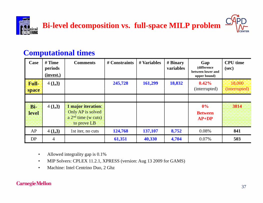
Bi-level decomposition vs. full-space MILP problem
Case # Time Comments # Constraints # Variables # Binary Gap CPU time
Computational timesCase # Time
periods(invest.)
Comments # Constraints # Variables # Binaryvariables
Gap(difference
between lower and upper bound)
CPU time (sec)
Full- 4 (1,3) 245,728 161,299 18,832 0.42%(interrupted)
18,000(interrupted)space (interrupted) (interrupted)
Bi-level
4 (1,3) 1 major iteration:Only AP is solved
0%Between
3814level
a 2nd time (w cuts) to prove LB
Between AP+DP
AP 4 (1,3) 1st iter, no cuts 124,768 137,107 8,752 0.08% 841
DP 4 61,351 40,330 4,704 0 07% 503DP 4 61,351 40,330 4,704 0.07% 503
• Allowed integrality gap is 0.1% • MIP Solvers: CPLEX 11.2.1, XPRESS (version: Aug 13 2009 for GAMS)
37
• Machine: Intel Centrino Duo, 2 Ghz
- The uncertainty challenge:
Sh i i b t ti i tiShort term uncertainties: robust optimizationComputation time comparable to deterministic models
Long term uncertainties: stochastic programmingComputation time one to two orders of magnitude larger than deterministic modelsthan deterministic models
38
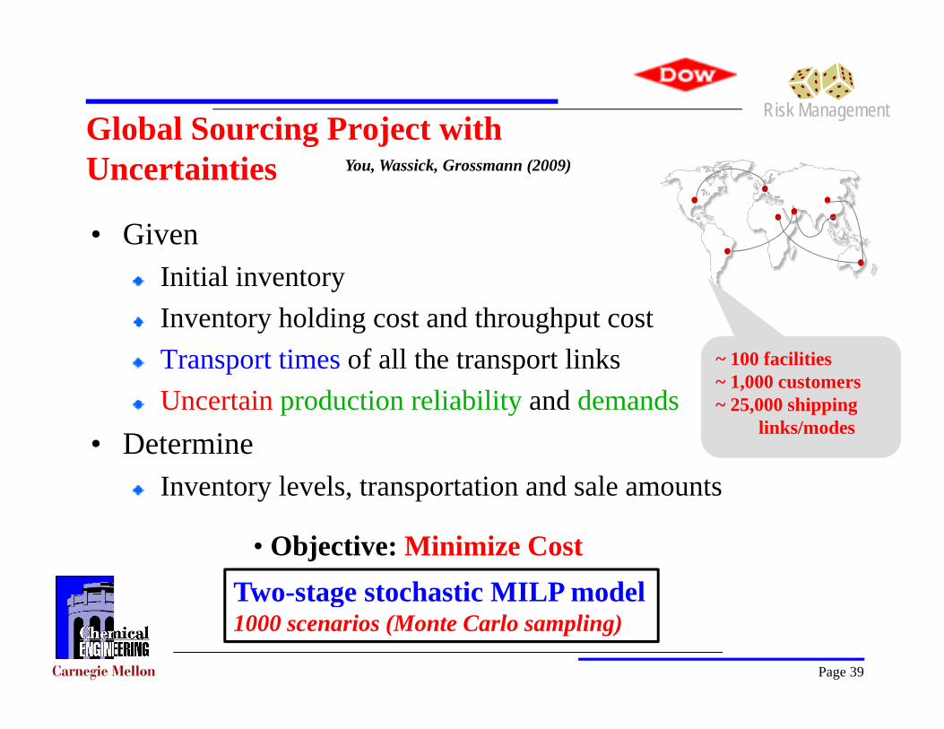
Risk ManagementGlobal Sourcing Project withGlobal Sourcing Project with Uncertainties
Gi
You, Wassick, Grossmann (2009)
• GivenInitial inventoryInventory holding cost and throughput cost
~ 100 facilities~ 1,000 customers~ 25,000 shipping
Inventory holding cost and throughput costTransport times of all the transport linksUncertain production reliability and demands 25,000 shipping
links/modesp y
• DetermineInventory levels, transportation and sale amounts
• Objective: Minimize CostTwo-stage stochastic MILP model
Page 39
Two-stage stochastic MILP model1000 scenarios (Monte Carlo sampling)

Risk Management
MILP P bl SiMILP Problem Size
DeterministicStochastic
ProgrammingCase Study 1 Deterministic
ModelProgramming
Model1,000 scenarios
# of Constraints 62 187 52 684 187# of Constraints 62,187 52,684,187# of Cont. Var. 89,014 75,356,014# of Disc. Var. 7 7
Impossible to solve directlytakes 5 days by using standard L-shaped Bendersy y g ponly 20 hours with multi-cut version Benders30 min if using 50 parallel CPUs and multi-cut version
Page 40

Risk Management
Simulation Results to Assess Benefits Stochastic Model
Stochastic Planner vs Deterministic Planner
11
12Stochastic SolnDeterministic SolnAverage
5 70±0 03%
Stochastic Planner vs Deterministic Planner
10
11
)
5.70±0.03%cost saving
9
Cos
t ($M
M)
7
8
C
61 10 19 28 37 46 55 64 73 82 91 100
i
Page 41
Iterations

Off h ilfi ld h i l i d t i t
Optimal Development Planning under Uncertainty
Decisions: N b d it f TLP/FPSO f iliti
facilities
Offshore oilfield having several reservoirs under uncertaintyMaximize the expected net present value (ENPV) of the project
Tarhan, Grossmann (2009)
Number and capacity of TLP/FPSO facilities Installation schedule for facilities Number of sub-sea/TLP wells to drill Oil production profile over time Oil production profile over time
TLP FPSO
ReservoirsReservoirswells
Uncertainty:
Initial productivity per well
42
Size of reservoirs Water breakthrough time for reservoirs
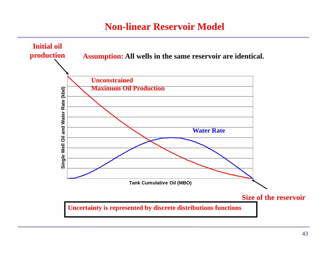
Non-linear Reservoir Model
Initial oil
U t i d
Initial oil production Assumption: All wells in the same reservoir are identical.
Rat
e (k
bd)
Unconstrained Maximum Oil Production
Oil
and
Wat
er
Water Rate
Sing
le W
ell
Tank Cumulative Oil (MBO)
Size of the reservoirUncertainty is represented by discrete distributions functions
43
Uncertainty is represented by discrete distributions functions

Decision Dependent Scenario TreesEndogeneous uncertainty: size field
Invest in F in year 1 Invest in F
Assumption: Uncertainty in a field resolved as soon as WP installed at field
Invest in F in year 5
g y
H
ves
Size of F: M L
Invest in F
Scenario tree
HSize of F: LM
4444
Scenario tree – Not unique: Depends on timing of investment at uncertain fields– Central to defining a Stochastic Programming Model

Multi-stage Stochastic Nonconvex MINLP
M i i P b bilit i ht d f NPV t i t iMaximize.. Probability weighted average of NPV over uncertainty scenariossubject to
Equations about economics of the model Surface constraints Surface constraints Non-linear equations related to reservoir performance Logic constraints relating decisions
if there is a TLP available, a TLP well can be drilled
Every scenario,
time period
Non-anticipativity constraintsNon-anticipativity prevents a decision being taken now from using information that will only become available in the future
Every pair scenarios,
time periodDisjunctions (conditional constraints)
Problem size MINLP increases ti ll ith b f ti i d
Decomposition algorithm:L l i &
time period
exponentially with number of time periodsand scenarios
Lagrangean relaxation & Branch and Bound
45

Multistage Stochastic Programming Approach
RS: Reservoir sizeOne reservoir, 10 years, 8 scenarios
RS: Reservoir sizeIP: Initial ProductivityBP: Breakthrough Parameter
E[NPV] = $4.92 x 10⁹
year 1
Build 2 small FPSO’sDrill 12 sub-sea wells
year 1
year 212 subsea wells
Low RSLow IP
High RSHigh IP
High RSLow IP
Low RSHigh IP
4 small FPSO’s, 5 TLP’
5 small FPSO’s, 3 TLP’
2 small FPSO’s, 2 TLP’
Mean RSMean IP
5 TLP’s12 subsea wells
3 TLP’s2 TLP’s3 subsea wells
S l ti b ildi 2 ll FPSO’ i th fi t d th dd
46
Solution proposes building 2 small FPSO’s in the first year and then add new facilities / drill wells (recourse action) depending on the positive or negative outcomes.

RS: Reservoir size
Multistage Stochastic Programming ApproachOne reservoir, 10 years, 8 scenarios
RS: Reservoir sizeIP: Initial ProductivityBP: Breakthrough Parameter
E[NPV] = $4.92 x 10⁹
year 1
Build 2 small FPSO’sDrill 12 sub-sea wells
year 1
year 212 subsea wells
Low RSLow IP
High RSHigh IP
High RSLow IP
Low RSHigh IP
4 small FPSO’s, 5 TLP’
5 small FPSO’s, 3 TLP’
2 small FPSO’s, 2 TLP’
Mean RSMean IP
5 TLP’s12 subsea wells
3 TLP’s2 TLP’s3 subsea wells
year 36 subsea wells, 18 TLP wells
12 subsea wells, 30 TLP wells
12 subsea wells6 subsea wells 6 subsea wells,
12 TLP wells y
year 4High BP Low BP
18 TLP wells
High BP Low BP High BP Low BP High BP Low BP
30 TLP wells12 TLP wells
Mean BP
S l ti b ildi 2 ll FPSO’ i th fi t d th dd
8 91 2 6 73 4 5
47
Solution proposes building 2 small FPSO’s in the first year and then add new facilities / drill wells (recourse action) depending on the positive or negative outcomes.

Distribution of Net Present Value
8
10
4
6t P
rese
nt V
alue
($ x
10
9 )
0
2
1 2 3 4 5 6 7 8 9
Net
-2
Scenarios
Deterministic Mean Value = $4.38 x 10⁹
Multistage Stoch Progr = $4.92 x 109 => 12% higher and more robustg g g
Computation: Algorithm 1: 120 hrs; Algorithm 2: 5.2 hrsNonconvex MINLP: 1400 discrete vars, 970 cont vars, 8090 Constraints
48
No co ve N : 00 d sc ete va s, 970 co t va s, 8090 Co st a ts

Economics vs. performance?
Multiobjective Optimization Approach
49

Optimal Design of Responsive Process Supply ChainsObjective: design supply chain polystyrene resisns under responsive and economic criteria You, Grossmann (2008)
50
Possible Plant SiteSupplier Location
Distribution CenterCustomer Location

Production Network of Polystyrene Resins
Example
Production Network of Polystyrene ResinsThree types of plants:
Plant I: Ethylene + Benzene Styrene (1 products)Plant I: Ethylene + Benzene Styrene (1 products)
Plant II: Styrene Solid Polystyrene (SPS) (3 products)
Plant III: Styrene Expandable Polystyrene (EPS) (2 products)
Basic Production Network
y p y y ( ) ( p )
Multi Product
Single Product
Multi Product
Source: Data Courtesy Nova Chemical Inc. http://www.novachem.com/
Multi Product
51

Potential Network SuperstructureExample
IL
CASPSPlant Site MI
NVWA
TXI
II
III
CAEthylene
Benzene
StyreneSPS
EPS AZTX
III
II
IEthylene
BenzeneStyrene Styrene
SPS
EPS
OK
Plant Site TX Plant Site CA
GANC
TX
Plant Site TX Plant Site CA
IEthylene
Benzene
Styrene PAFL
OH
MS
LA IIIEPSPlant Site LA
MA
MN
IAAL
EPS
52
MN
Suppliers Plant Sites Distribution Centers Customers

Lead Time under Demand Uncertainty
Model & Algorithm
Lead Time under Demand Uncertainty
Inventory (Safety Stock)
53

Bi-criterion Multiperiod MINLP Formulation
Model & Algorithm
• Objective Function:Choose Discrete (0-1), continuous variables
Bi criterion Multiperiod MINLP Formulation
Max: Net Present Value
Min: Expected Lead time• Constraints:
Bi-criterion
Network structure constraintsSuppliers – plant sites RelationshipPlant sites – Distribution Center Cyclic scheduling constraints
i iInput and output relationship of a plantDistribution Center – Customers Cost constraint
Assignment constraintSequence constraintDemand constraintProduction constraint Operation planning constraintsCost constraint
Probabilistic constraintsChance constraint for stock out
p p gProduction constraintCapacity constraintMass balance constraintD d t i t (reformulations)Demand constraintUpper bound constraint
54

Pareto Curves – with and without safety stock
Example
750
Pareto Curves with and without safety stock
600
650
700
500
550
600
NPV
(M$)
More Responsive
400
450
N
300
350
1 5 2 2 5 3 3 5 4 4 5 5 5 5
with safety stockwithout safety stock
1.5 2 2.5 3 3.5 4 4.5 5 5.5Expected Lead Time (day)
55

Safety Stock Levels - Expected Lead Time
Example
200EPS in DC2
Safety Stock Levels Expected Lead Time
150
T)
EPS in DC2SPS in DC2EPS in DC1SPS in DC1
100
tock
(10^
4 T
More inventory, more responsive
50Safe
ty S
t more responsive
Responsiveness
01 51 2 17 2 83 3 48 4 14 4 81.51 2.17 2.83 3.48 4.14 4.8
Expceted Lead Time (day)
56

Other Issues / Future Directions
1. Integration of control with planning and scheduling Bhatia, Biegler (1996), Perea, Ydstie, Grossmann (2003), Flores, Grossmann (2006), Prata, Oldenburg, Kroll, Marquardt (2008) , Harjunkoski, Nystrom, Horch (2009)
2 Optimization of entire supply chains
Prata, Oldenburg, Kroll, Marquardt (2008) , Harjunkoski, Nystrom, Horch (2009)
Challenge: Effective solution of Mixed-Integer Dynamic Optimization (MIDO)
2. Optimization of entire supply chainsChallenges: - Combining different models (eg maritime and vehicle transportation, pipelines)
C f C d (2004) R l M t B b Pó Fi lh Pi h i (2006)
3 D i d O ti f S t i bl S l Ch i
Cafaro, Cerda (2004), Relvas, Matos, Barbosa-Póvoa, Fialho, Pinheiro (2006)- Advanced financial models
Van den Heever, Grossmann (2000), Guillén, Badell, Espuña, Puigjaner (2006),
3. Design and Operation of Sustainable Supply ChainsChallenges:Biofuels, Energy, Environmental
l l b l d (2011) G llé G álb (2011) G S d (2011)
57
Elia, Baliban, Floudas (2011) Guillén-Gosálbez (2011), You, Tao, Graziano, Snyder (2011)

Conclusions
1. Enterprise-wide Optimization area of great industrial interestG t i i t f ff ti l i l l h iGreat economic impact for effectively managing complex supply chains
2. Key components: Planning and SchedulingM d li h ll
3 C t ti l h ll li i
Modeling challenge:Multi-scale modeling (temporal and spatial integration )
3. Computational challenges lie in:a) Large-scale optimization models (decomposition, advanced computing )b) Handling uncertainty (stochastic programming)
58