HAL Id: hal-00214209https://hal.archives-ouvertes.fr/hal-00214209

Submitted on 23 Jan 2008

HAL is a multi-disciplinary open accessarchive for the deposit and dissemination of sci-entific research documents, whether they are pub-lished or not. The documents may come fromteaching and research institutions in France orabroad, or from public or private research centers.

L’archive ouverte pluridisciplinaire HAL, estdestinée au dépôt et à la diffusion de documentsscientifiques de niveau recherche, publiés ou non,émanant des établissements d’enseignement et derecherche français ou étrangers, des laboratoirespublics ou privés.

On the effective behavior of nonlinear inelasticcomposites: I. Incremental variational principles.

Noël Lahellec, Pierre Suquet

To cite this version:Noël Lahellec, Pierre Suquet. On the effective behavior of nonlinear inelastic composites: I. Incre-mental variational principles.. Journal of the Mechanics and Physics of Solids, Elsevier, 2007, 55 (9),pp.1932-1963. �10.1016/j.jmps.2007.02.003�. �hal-00214209�

On the effective behavior of

nonlinear inelastic composites:

I. Incremental variational principles.

Noel LAHELLEC a, Pierre SUQUET a,∗

aLaboratoire de Mecanique et d’Acoustique, 31 chemin Joseph Aiguier, 13402Marseille cedex 20, France

E-mail: lahellec@lma.cnrs-mrs.fr, suquet@lma.cnrs-mrs.fr

Abstract

A new method for determining the overall behavior of composite materials com-prised of nonlinear inelastic constituents is presented. Upon use of an implicit time-discretization scheme, the evolution equations describing the constitutive behaviorof the phases can be reduced to the minimization of an incremental energy func-tion. This minimization problem is rigorously equivalent to a nonlinear thermoe-lastic problem with a transformation strain which is a nonuniform field (not evenuniform within the phases). In this first part of the study the variational techniqueof Ponte Castaneda is used to approximate the nonuniform eigenstrains by piece-wise uniform eigenstrains and to linearize the nonlinear thermoelastic problem. Theresulting problem is amenable to simpler calculations and analytical results for ap-propriate microstructures can be obtained. The accuracy of the proposed scheme isassessed by comparison of the method with exact results.

Key words: Composite, homogenization, nonlinear viscoelasticity,elasto-viscoplasticity, variational method, random micro-structure,Hashin-Shtrikman estimates.

1 Introduction

This study is devoted to the overall response of nonlinear composites com-prised of phases which, when deformed, have a partly reversible and partlyirreversible behavior. This is the case of nonlinear viscoelastic constituents,where both elastic and viscous effects are always present and coupled, and of

∗ Corresponding author

Preprint submitted to Elsevier Science 23 January 2008

elasto-viscoplastic or elasto-plastic constituents for which there exists a do-main in stress space where the material behaves in a purely elastic manner,and more generally of most engineering materials (Lemaitre and Chaboche,1994).

Reversible effects are associated with a free-energy density which depends onlyof the state variables of the material. It consists of all the energy available ina given state of the system (at a given material point). The driving forces(or thermodynamic forces) responsible for the evolution of the system, char-acterized by changes in the state variables, are obtained by derivation of thefree-energy with respect to the state variables (Gibbs relations).

On the other hand, irreversibility is characterized by dissipation along an evo-lution path of the system. Changes in the state variables are governed by theaforementioned driving forces. A convenient (and commonly used) formulationof the corresponding evolution equations for dissipative materials is based onthe assumption that they can be derived from a dissipation potential (see Rice,1970, Halphen and Nguyen, 1975 or Germain et al., 1983, for a review). Thepresent study is conducted in this setting of constitutive relations which canbe deduced from two potentials, the free-energy function and the dissipationpotential.

The problem of predicting the effective response of heterogeneous materialscomprised of elasto-plastic or elasto-viscoplastic phases has been mainly ad-dressed in the literature by numerical means (see Christman et al., 1989, Baoet al., 1991, Fish and Shek, 1998, Gonzalez et al., 2004, to cite only a few).However numerical simulations are not the objective of the present study butwill rather be used to assess the accuracy of the theoretical methods hereafterproposed.

Regarding theoretical or analytical predictions, which are our main objectivehere, several directions of research have been explored and it is worth men-tioning how they differ from the present study.

(1) Elasto-plastic composites are mostly considered in the literature in theframework of a deformation theory in which the actual incremental con-stitutive relations for the phases are replaced by nonlinear elastic re-lations. Within this approximation, classical micromechanical schemes,such as the secant method, have been applied (see Chu and Hashin, 1971,Berveiller and Zaoui, 1979, among others), as well as more recent homog-enization techniques for nonlinear composites with one potential (see forinstance Li and Ponte Castaneda, 1993, Suquet, 1997 Bardella, 2003 andGonzalez et al., 2004, for particle-reinforced composites). These recenthomogenization methods are based on the existence of a single potentialand make use of the variational characterization of the local fields and of

2

the effective potential. They include on the one hand rigorous bounds ob-tained by variational methods, such as the generalization by Talbot andWillis (1985) of the Hashin-Shtrikman technique, the variational methodof Ponte Castaneda (1992) and its subsequent interpretation as a modi-fied secant method by Suquet (1995), Suquet (1997), and other equivalentvariational schemes based on convexity inequalities (Suquet, 1993, Olson,1997). They also include estimates, which are exact to second-order inthe contrast of the phases, obtained by taking a Taylor expansion of thepotential (Ponte Castaneda, 1996, Ponte Castaneda, 2002). The notionof a linear comparison composite is central in these studies.

However, the approximation on which the deformation theory of plas-ticity is based is legitimate only when the loading is locally proportional(i.e. at all material points in the volume element), the axes of princi-pal stresses remaining fixed and the local stress being monotonically in-creased with no unloading. This situation is very rarely met in compositematerials. The approximation of constant principal directions of stress ateach material point at the local level is a reasonable approximation (butby no means an exact result) when the overall loading is itself propor-tional but it becomes unrealistic in other circumstances when the loadingpath involves a rotation of the principal axis of macroscopic stress. Simi-larly, the assumption of monotone loading (at each local material point)is acceptable (but not exact) as long as the macroscopic stress is ap-plied monotonically, but is completely unrealistic under general loadingconditions with loading and unloading sequences. These limitations havemotivated the present study where the approximation of a deformationtheory is not made and where the incremental form of the actual consti-tutive relations is taken into account.

(2) The Transformation Field Analysis (TFA) proposed by Dvorak (1992)and implemented by different authors (Dvorak et al., 1994, Fish and Shek,1998 among others) offers an elegant direction of research, in which theincremental form of the constitutive relations is preserved. In this ap-proach, the plastic strain (or more generally the transformation strainwhich can be due to various effects such as thermal effects, plasticity,phase transformation, damage....) is assumed to be uniform within eachindividual phase in the composite. However, as is now well-recognized(Suquet, 1997, Chaboche et al., 2001), this model leads to excessivelystiff predictions (which can be softened by subdividing each phase intosubdomains, at the expense of increasing the complexity of the model).This excessive stiffness is due to the assumed uniformity of the trans-formation strain in each phase which is unrealistic in practice (except invery particular situations such as laminates or nonlinear inclusions in alinear matrix). As will be shown in appendix A, the TFA can be obtainedas a special case of the present theory by enforcing the fields of internalvariables to be uniform per phase, which is a very crude approximationfrom which the present study is free.

3

(3) Linearization of the constitutive relations for nonlinear viscoelastic het-erogeneous materials have been proposed by Li and Weng (1997), Mas-son and Zaoui (1999), Brenner et al. (2002), Levesque et al. (2004) andBrenner and Masson (2005) (among others) to reduce the problem to asimpler one for a linear viscoelastic comparison composite. The presentstudy is also based on an appropriate linearization of the constitutive re-lations and the two parts of the paper make use of two different types oflinearization. But an essential difference with Masson and Zaoui (1999),Brenner et al. (2002) and Brenner and Masson (2005) is that in theseprevious studies, the stress history is computed at each time step fromthe initial time t = 0 (and not from the previous time step) to the presenttime. In other words, assume that the loading is imposed on a time in-terval [0, T ] discretized into successive time-steps tn, tn+1... and that oneis interested in the response of the composite at tn+1, knowing the over-all stress and strain at time tn. According to these previous studies, onewould have to determine an “equivalent” linear viscoelastic composite attime tn+1 and compute the whole history of the stress and strain from 0to tn+1 without using the stress and strain determined at time tn (see forinstance Levesque et al. , 2004). By contrast, the present study is a truestep-by-step procedure and is radically different from the previous ones.Here, the strain and internal variables in the composite are determinedat time tn+1 using the strain and internal variables at time tn and theloading conditions at time tn+1.

(4) The special case of linear viscoelastic composites, which is a particularcase of the class of materials considered here for which the dissipationpotential is a quadratic function, deserves a special mention. There ex-ists an abundant literature on the subject, mostly based on the corre-spondence principle (see for instance Hashin, 1970). In this approach,the equations governing the local state and the effective properties oflinear viscoelastic composites are, after application of the Laplace trans-form, completely parallel to that of linear elastic composites with complexmoduli. Theoretical results and predictive schemes initially developed forelastic composites can be therefore extended to viscoelastic compositesby the correspondence principle. One of these theoretical results is thatshort memory effects in the individual constituents give rise, after homog-enization, to long memory effects in the composite (Sanchez-Hubert andSanchez-Palencia, 1978 and Suquet, 1987). As a consequence of these longmemory effects, the overall stress at time t depends on the whole historyof the strain between times 0 and t. The exact effective constitutive rela-tions require the storage at time t of an infinite number of informationscorresponding to the overall strains at all previous times. This result isconsistent with a more general result of Suquet (1987) which shows thatthe exact effective relations of elasto-viscoplastic composites requires, ingeneral, the knowledge at time t of an infinite number of internal vari-ables. This theoretical result is of limited practical use since a realistic

4

effective constitutive relation should require only the knowledge of a finite(and hopefully limited) number of informations. But this exact result hasthe merit of highlighting the complexity of the homogenization procedurewhen the local constituents exhibit both elastic and dissipative effects.Reducing the size of necessary information cannot be achieved exactly ingeneral, but only within certain approximations. Therefore the questionwhich we are left with is not that of finding an exact theory (too am-bitiou)s, but that of finding a set of approximations leading to accurateresults and to an easy implementation.

The paper is organized as follows. The constitutive relations of the individualconstituents are presented in section 2.1. An incremental variational principlefor a time-discretized version of the resulting evolution equations is derived insection 2.2 at the local level and in section 3.2 at the level of the composite.Variational incremental principles for dissipative, or elasto-plastic systems,have been known for some time but have received for some time only littleattention. One of the first occurrence of such a variational principle in a formclose to the one that will be used here, can be found in Mialon (1986) for rate-independent systems (other variational approaches can be found in Simo andHughes, 1998, chapter 4 and the references herein). Mialon (1986) establisheda variational principle for bodies comprised of generalized standard materialsand used it to derive several computational algorithms for elasto-plasticitywith (or without) hardening. These algorithms (but not the variational prin-ciples themselves) were subsequently applied to homogenization problems inplasticity by Marigo et al. (1987). Recently (and independently) variationalprinciples similar in spirit to that of Mialon, but much more general in thesense that they apply also to rate-dependent elasto-viscoplastic materials at fi-nite strains, have been derived by Ortiz and Stainier (1999).A renewed interestfor incremental variational principles followed this paper, which not only gavenew directions for the time integration of rate-dependent or rate-independentdissipative structures, but also opened new perspectives in the understand-ing of the formation of microstructures in elastoplastic materials (Ortiz andRepetto, 1999). The importance of these more recent variational principlesin homogenization of nonlinear materials has also been recognized by Miehe(2002) and Miehe et al. (2002) who made several computational applicationsof these principles to finite strain plasticity of composites or polycrystals withevolving microstructures.

In the present study, these variational principles are used to derive approxi-mate but almost analytical schemes for the prediction of the global responseand first and second-order statistics of the local fields in nonlinear dissipativecomposites. The method is general and applies both to nonlinear viscoelasticconstituents, where elastic and viscous effects are always coupled, and elasto-viscoplastic constituents (where there exists a domain in stress space insidewhich the material behaves in a purely elastic manner). For brevity, the the-

5

ory is illustrated here only in the case of nonlinear viscoelastic materials, butapplications to elasto-viscoplastic materials do exist and will be publishedseparately.

The exact and time-discretized effective constitutive relations are recalled insection 3. The time-discretization allows us to reduce the problem with twopotentials to the minimization of a single potential for a nonlinear thermoe-lastic body subjected to nonuniform eigenstrains (not even uniform withineach individual phase). The proposed approximation consists in replacingthe nonuniform eigenstrains by piecewise uniform (within in each individ-ual phase) eigenstrains and in linearizing the thermoelastic composite. Thisis done by a procedure close to the modified secant method of Suquet (1995)(equivalent to the variational method of Ponte Castaneda (1992)). The re-sulting thermoelastic problem is therefore a classical problem for a N -phasecomposite. The accuracy of the proposed scheme is assessed in section 5 bycomparing the predictions of the scheme with exact results for two or three-dimensional microstructures.

2 Individual constituents

2.1 Generalized standard materials

The composite materials considered in this study are comprised of individualconstituents exhibiting a dissipative behavior which can be modelled in themore general framework of constitutive relations deriving from two thermo-dynamic potentials. The main ingredients for such a model are threefold :

a) A finite number of internal variables α which, in addition to the observablestrain ε, describe the internal state of the material. Attention is limited hereto infinitesimal strains.

b) A free-energy function w(ε, α) which gives, for each possible state (ε, α)of the system (material) the energy available to trigger its evolution. Thedriving forces associated with the state variables are :

σ =∂w

∂ε(ε, α), A = −

∂w

∂α(ε, α). (1)

c) A dissipation potential ϕ(α) which relates the evolution of the internal vari-ables α to the driving forces :

A =∂ϕ

∂α(α), or equivalently α =

∂ϕ∗

∂A(A), (2)

6

where ϕ∗ is the Legendre transform of ϕ. When the two potentials w and ϕ areconvex functions of their arguments (ε, α) and α respectively), the materialgoverned by (1) and (2) is said to be a generalized standard material (Halphenand Nguyen, 1975, Germain et al., 1983).

Upon elimination of A between (1) and (2), the constitutive relations of thematerials under consideration can be re-written as a system of two coupledequations, one of them being a differential equation in time :

σ =∂w

∂ε(ε, α),

∂w

∂α(ε, α) +

∂ϕ

∂α(α) = 0. (3)

Most classical nonlinear viscoelastic or elasto-viscoplastic models can be for-mulated in this general framework by appropriate choices of the potentials wand ϕ (Germain et al., 1983, Lemaitre and Chaboche, 1994).

2.2 Incremental potential

The present section presents the extension to rate-dependent systems of thevariational principle of Mialon (1986) and Ortiz and Stainier (1999) in thesimplified framework of infinitesimal strains and of a fully implicit time-integration scheme.

The time derivative in (3) can be approximated by a difference quotient afteruse of an implicit Euler-scheme. The time interval of study [0, T ] is discretizedinto time intervals t0 = 0, t1, ...., tn, tn+1, ..., tN = T . The time step tn+1 − tnis denoted by ∆t (its dependence on n is omitted for simplicity). The time-derivative of a function f at time tn+1 is replaced by the difference quotient(f(tn+1) − f(tn))/∆t and the constitutive relations are written at the end ofthe time step. This time-discretization procedure applied to (3) leads to thediscretized system :

σn+1 =∂w

∂ε(εn+1, αn+1),

∂w

∂α(εn+1, αn+1) +

∂ϕ

∂α

(αn+1 − αn

∆t

)= 0. (4)

Assuming that the fields σn, εn and αn are known at time tn, the unknownsσn+1, εn+1 and αn+1 at time tn+1 solve this discretized version of the system(3). It is readily seen by taking the derivative of J defined in (5) with respectto α that the second equation in (4) is the Euler-Lagrange equations for thefollowing variational problem (with solution αn+1):

Infα

J(εn+1, α), J(ε, α) = w(ε, α) + ∆t ϕ(

α − αn

∆t

). (5)

7

Then, defining the following potential :

w∆(ε) = Infα

J(ε, α), (6)

we obtain the following remarkable result which gives the stress as the deriva-tive of a single potential with respect to the strain :

σn+1 =∂w∆

∂ε(εn+1). (7)

J and w∆ are respectively called the incremental potential and the condensedincremental potential of the constituent under consideration.

In order to prove that relation (7) follows from (6) and (4), we note that thederivative of w∆ with respect to ε reads as :

∂w∆

∂ε(ε) =

∂J

∂ε(ε, α) +

∂J

∂α(ε, α) :

∂α

∂ε, (8)

where α(ε) denotes the solution of the infimum problem in (6). The last termin (8) vanishes by virtue of the stationarity of J with respect to α, and weare left with :

∂w∆

∂ε(ε) =

∂J

∂ε(ε, α) =

∂w

∂ε(ε, α). (9)

This relation, applied with ε = εn+1 gives (7).

Remark 1 : Under the assumption that w and ϕ are convex functions oftheir arguments, the incremental potential J is a convex function of (α, ε)and the condensed incremental potential w∆ is a convex function of ε. Thelatter property follows from a general result (Ekeland and Temam, 1976, forinstance)

Let Φ(u, p) be a convex function on V × Y (where V and Y are two Banachspaces) with values in R ∪ {+∞} , and let h be defined on Y as

h(p) = Infu∈V

Φ(u, p).

Then h is a convex function.

In the present context, (u, p) = (α, ε), Φ = J and h = w∆.

Furthermore, when w and ϕ are twice-differentiable functions, w∆ is also twice-differentiable and its second derivative can be expressed after a straightforwardcalculation as :

∂2w∆

∂ε2(ε) = Lεε − Lεα :

(Lαα +

1

∆tLv

)−1

: Lαε, (10)

8

where :

Lεε =∂2w

∂ε2, Lεα =

∂2w

∂ε∂α, Lαε =

∂2w

∂α∂ε, Lαα =

∂2w

∂α2et Lv =

∂2ϕ

∂α2 .

The convexity of w∆ can alternatively be deduced from (10). Indeed, theconvexity of w and ϕ imply (all inequalities should be understood in the senseof positivity for symmetric quadratic forms) :

Lεε − Lεα : (Lαα)−1 : Lαε ≥ 0, Lv ≥ 0,

and therefore

Lεε − Lεα :(Lαα +

1

∆tLv

)−1

: Lαε ≥ Lεε − Lεα : (Lαα)−1 : Lαε ≥ 0.

3 Composite materials. Effective behavior

3.1 Local problem

A representative volume element (r.v.e.) V of the composite is comprised of Nphases occupying domains V (r) with characteristic functions χ(r) and volumefraction c(r). Each individual phase is governed by the differential equations (3)with potentials w(r) and ϕ(r). The free-energy w and the dissipation potentialϕ at position x are given by:

w(x, ε, α) =N∑

r=1

χ(r)(x)w(r)(ε, α), ϕ(x, α) =N∑

r=1

χ(r)(x)ϕ(r)(α). (11)

The r.v.e. V is subjected to a path of macroscopic strain E(t) and the localproblem which is solved by the local fields σ(x, t), ε(x, t) and α(x, t) readsas :

σ =∂w

∂ε(ε, α),

∂w

∂α(ε, α) +

∂ϕ

∂α(α) = 0 for (x, t) ∈ V × [0, T ],

div σ = 0 for (x, t) ∈ V × [0, T ],

〈ε(t)〉 = E(t) + boundary conditions on ∂V.

(12)All fields σ, ε, α depend on x and t. The bracket 〈.〉 denotes spatial averagingover V . For definiteness, periodic boundary conditions are imposed on theboundary of V .

The homogenized or effective response of the composite along the path of

9

prescribed strain {E(t), t ∈ [0, T ]} is the history of average stress {Σ(t), t ∈[0, T ]} where Σ(t) = 〈σ(x, t)〉.

3.2 Effective incremental potential

Upon discretization of the time interval [0, T ], the discretized version of thelocal problem (12) can be written with the help of (7) as :

σn+1 =∂w∆

∂ε(εn+1), div σn+1 = 0, in V,

〈εn+1〉 = En+1 + boundary conditions on ∂V.

(13)

where the incremental potentials J and w∆ read as :

J(ε, α, x) =N∑

r=1

(w(r)(ε, α) + ∆t ϕ(r)

(α − αn(x)

∆t

))χ(r)(x),

w∆(ε, x) = Infα

J(ε, α, x).

(14)

The average stress Σn+1 = 〈σn+1〉 satisfies :

Σn+1 =∂w∆

∂E(En+1) , (15)

where the effective energy w∆ has the variational characterization :

w∆ (En+1) = Inf〈ε〉=En+1

〈w∆(ε)〉 = Inf〈ε〉=En+1

⟨Infα

J(ε, α)⟩

. (16)

To prove the validity of (15), we compute the derivative of w∆ with respectto E :

∂w∆

∂E(En+1) =

⟨∂J

∂ε:

∂ε

∂E

⟩+

⟨∂J

∂α:

∂α

∂E

⟩. (17)

The second term vanishes (stationarity of J with respect to α) and the firstterm gives, thanks to the relation σ = ∂J/∂ε and Hill’s lemma :

⟨σn+1 :

∂ε

∂E

⟩= 〈σn+1〉 :

⟨∂ε

∂E

⟩= 〈σn+1〉 = Σn+1.

Thanks to this variational characterization, the homogenization of the evo-lution problem (12) is reduced to the variational problem (16). The latterproblem amounts to finding the effective energy w∆ of a composite materialwith one potential w∆. Two important things are worth noticing about thiscondensed potential :

10

1. The condensed potential w∆ is not explicitly known and is certainly non-quadratic.

2. The condensed potential w∆ depends on x not only through the charac-teristic functions χ(r)(x) but also through the fields α(x) and αn(x). Inother words w∆(ε) cannot be put under the familiar form (11).

The first point makes the variational problem (16) strongly reminiscent of theproblem of nonlinear composites composed of N different phases governed bya single potential. However the second point shows that the problem at handis more complicated than the latter one. Even the full incremental potential Jdoes not depend only on the phase r but also depends on the internal variableαn at time tn which may be completely inhomogeneous, even within eachsingle phase.

3.3 Orientation for the rest of the study

Two objectives will be pursued in the rest of this study :

1. First, in order to make contact with recent work on nonlinear compositematerials with a single nonquadratic potential, one has to approximate thepotentials w∆ or J which depend on the position through αn(x), by po-tentials in the form (11). This is more easily achieved with J than withw∆. The approximation consists in replacing in the expression (14) the fieldαn(x) in phase r by an effective internal variable α(r)

n which remains to bedefined. The resulting problem is then close to that for a N -phase nonlinearcomposite, but not completely identical since there remains an additionalminimization over the field α.

A first natural guess for the effective internal variable α(r)n could be to

consider the fields αn(x) and α(x) to be piecewise uniform within eachindividual phase. As shown in appendix A, this choice leads precisely tothe Transformation Field Analysis (TFA) of Dvorak (1992). However, it hasbeen observed in the literature (Suquet, 1997, Chaboche et al., 2001) thatthe TFA may lead to inaccurate results in certain circumstances. Thereforethe present approach goes beyond piecewise uniform fields of internal vari-ables and accounts for the first and the second moments of these variablesin each individual phases.

2. Second, a strategy has to be chosen in order to approximate J in the vari-ational problem (16) by a quadratic function. As is known from the studyof nonlinear composites with only one potential, several procedures withdifferent degree of complexity and accuracy are available to this effect. Twoof them, which have proven to be flexible and efficient in the latter context,have been explored in the present study. The first approach, presented insection 4 derives from the variational method of Ponte Castaneda (1992)

11

and its variant called the modified secant method (Suquet, 1995, PonteCastaneda and Suquet, 1998). It makes use of an isotropic linear compar-ison composite. In the present context the linear comparison composite iscomprised of isotropic, linearly viscoelastic phases.

The second approach, presented in the second part of this study, is basedon a generalization, due to Lahellec and Suquet (2004), of the second-ordermethod of Ponte Castaneda (1996). It makes use of an anisotropic linearcomparison composite and is presented in the second part of this study.

As will be seen the two above steps, finding an effective internal variablefor each phase and linearizing the constitutive relations, are not completelyindependent.

3.4 Working assumptions

For simplicity, several working assumptions will be made in the following.They are assumed to hold for each individual constituent in the composite.

H1: The internal state variable α is a symmetric, traceless, second-order ten-sorial variable which can be seen as the inelastic strain.

H2: The free energy w(r) is a quadratic function of ε and α.

For further simplicity it will be assumed that w(r) can be written as :

w(r)(ε, α) =1

2(ε − α) : L(r) : (ε − α), (18)

where the fourth-order tensor L(r) has minor and major symmetries :

L(r)ijkh = L

(r)jikh = L

(r)khij.

H3: The dissipation potential ϕ, which is a convex function of α, is assumedto be a function of the sole invariant αeq :

ϕ(r)(α) = φ(r)(αeq) where αeq =(

2

3α : α

)1/2

, (19)

It is further assumed that φ(r) can be written as

φ(r)(αeq) = f (r)(α2eq

),

where f (r) is a concave function of its scalar argument.

12

The secant viscosity ηsct of the constituent is defined as :

∂ϕ(r)

∂α(α) = 2η

(r)sct (αeq)α, (20)

and can be expressed in terms of the functions φ(r) and f (r) by the relations :

η(r)sct (αeq) =

1

3

φ′(r)(αeq)

αeq

=2

3f ′(r)(α2

eq). (21)

Remark 2 : Assumption H3 is met by standard potentials. For the sake ofsimplicity we shall restrict our attention to simple potentials with no accountof hardening effects. Consider for instance the power-law potential:

ϕ(r)(α) =σ

(r)0 ε0

(m + 1)

(αeq

ε0

)m+1

, with f (r)(x) =σ

(r)0

(m + 1)εm0

(x)m+1

2 . (22)

The associated constitutive relations describe a nonlinear viscoelastic behaviourand read as:

ε = M (r) : σ +3

2ε0

(σeq

σ(r)0

)ns

σeq

, M (r) =(L(r)

)−1, n =

1

m. (23)

The limiting case m = 0 (or equivalently n → +∞) corresponds to rate-independent elastoplasticity with yield stress σ0.

Similarly, a simple constitutive model for elasto-viscoplasticity is obtainedwhen the potential ϕ is chosen in the form :

ϕ(r)(α) = R(r)αeq +σ

(r)0 ε0

(m + 1)

(αeq

ε0

)m+1

. (24)

The corresponding constitutive relations read as :

ε = M (r) : σ +3

2ε0

((σeq − R(r))+

σ(r)0

)ns

σeq

, (25)

R(r) is the threshold below which the material behaves elastically and beyondwhich the strain-rate contains a viscous part.

As can be seen, the two potentials (22) and (24) have very similar formsalthough the second one has an elastic domain. Both potentials can be handledin almost the same manner (with the present variational method), exceptfor the numerical implementation where, for the second potential, it is moreconvenient to work with the inverse of the secant viscosity rather than withthe secant viscosity itself. For brevity, the theory will be illustrated in section5 only for nonlinear viscoelasticity.

13

Remark 3 : Free-energy potentials more general than (18) should be con-sidered to account for hardening effects (isotropic and kinematic hardening).This is possible within the very same framework but is left for future work.We would like to concentrate here on the simplest forms of the potentials.

4 Estimation of the effective incremental potential by a variationalmethod

In this section the determination of the effective incremental potential w∆ (16)is reduced to a simpler problem involving only a N -phase linear comparisoncomposite by means of a method inspired by the variational procedure ofPonte Castaneda (1992).

4.1 Variational procedure

The idea of the variational method is to add and subtract to the originalpotential J which is difficult to homogenize, an energy J0 (that for the linearcomparison composite) which is more amenable to homogenization, while thedifference J − J0 can still be estimated. Unlike the incremental potential J ,the energy J0 of the linear comparison composite is chosen to be quadraticand piecewise uniform,

J0(x, ε, α) =N∑

r=1

J(r)0 (ε, α)χ(r)(x),

where

J(r)0 (ε, α) = w(r)(ε, α) +

η(r)0

∆t(α − α(r)

n ) : (α − α(r)n ). (26)

In this expression η(r)0 and α(r)

n are uniform in phase r and will be chosenappropriately in the sequel. Note that J0 is the incremental potential for alinear viscoelastic comparison composite.

Let ∆J be the difference between J and J0 :

∆J(α) =N∑

r=1

∆t ϕ(r)(

α − αn

∆t

)−

η(r)0

∆t(α − α(r)

n ) : (α − α(r)n )

χ(r)(x).

(27)

14

Then (16) can be re-written as:

w∆ (E) = Inf〈ε〉=E

[Infα

〈J0(ε, α) + ∆J(α)〉]

≤ Inf〈ε〉=E

[Infα

〈J0(ε, α)〉 +⟨Sup

α

∆J(α)⟩]

.(28)

The last expression, where the supremum of ∆J over α is taken, provides arigorous upper bound for w∆. This upper bound can be too stiff in certaincircumstances as reported in Lahellec and Suquet (2006).

To improve on this prediction, it is worth noting that Ponte Castaneda andWillis (1999) and Ponte Castaneda (2002) have observed, in a different butsimilar context, that sharper estimates can be obtained by requiring onlystationarity of the “error function” (here ∆J) with respect to its argument(here α) :

w∆ (E) ≈ Inf〈ε〉=E

[Infα

〈J0(ε, α)〉 +⟨Stat

α∆J(α)

⟩]. (29)

We emphasize that the resulting expression has no upper bound character andis only an estimate (hopefully accurate) of w∆.

4.2 Linear viscoelastic constituents

To show how the method works independently of the nonlinearity associatedwith a general potential ϕ, let us first begin with the situation where theindividual constituents are linearly viscoelastic, following the lines of Lahellecand Suquet (2006) where additional results may be found. In this case, thedissipation potential ϕ is a quadratic function :

ϕ(r)(α) = η(r)α : α, (30)

and the stationarity condition, Statα

∆J(α), becomes :

Statα

N∑

r=1

η(r)

∆t(α − αn) : (α − αn) −

η(r)0

∆t(α − α(r)

n ) : (α − α(r)n )

χ(r)(x).

The solution α of the above stationarity problem satisfies in phase r :

2η(r) α − αn

∆t= 2η

(r)0

α − α(r)n

∆t, (31)

and therefore can be expressed in phase r as :

α(x) =αn(x) − θ(r)α(r)

n

1 − θ(r), (32)

15

where θ(r) = η(r)0 /η(r). With this relation, the last term in (29) can be evaluated

and the resulting estimate for w∆ reads :

w∆ (E) ≈ Inf〈ε〉=E

[Infα

〈J0(ε, α)〉]

+N∑

r=1

c(r)

⟨η(r)θ(r)

∆t(θ(r) − 1)(αn − α(r)

n ) : (αn − α(r)n )

⟩

r

(33)

where 〈.〉r denotes the spatial average over phase r and where θ(r) and α(r)n

remain to be determined.

4.2.1 Determination of θ(r) and α(r)n .

The estimate (33) can be optimized with respect to θ(r) and α(r)n . Stationarity

of the right-hand side of (33) with respect to these variables yields

∂

∂θ(r)

⟨J

(r)0 (ε, α) +

η(r)θ(r)

∆t(θ(r) − 1)(αn − α(r)

n ) : (αn − α(r)n )

⟩

r

= 0,

which implies, by virtue of the expression (26) of J(r)0 :

θ(r) = 1 ±

√√√√√

⟨(αn − α(r)

n ) : (αn − α(r)n )⟩

r⟨(α − α(r)

n ) : (α − α(r)n )⟩

r

. (34)

The sign in the above expression is left undetermined at this stage. It turnsout that taking the sign + corresponds to solving the problem (28) with asupremum. The sign − corresponds to an infimum and therefore to a rigorouslower bound for the effective condensed potential w∆.

Similarly, the stationarity condition over α(r)n reads :

∂

∂α(r)n

⟨J

(r)0 (ε, α) +

η(r)θ(r)

∆t(θ(r) − 1)(αn − α(r)

n ) : (αn − α(r)n )

⟩

r

= 0

⇒ α(r)n =

〈αn〉r + (θ(r) − 1) 〈α〉rθ(r)

, (35)

The two relations (34) and (35) show that the two unknowns θ(r) and α(r)n de-

pend only on the first and on the second moment of αn (information availablefrom time tn) and on the first and the second moment of α over the phase rwhich remain to be determined.

16

4.2.2 Minimization of J0(ε, α).

Once θ(r) and α(r)n are known through the relations (34) and (35), the function

J0 is completely specified and can be minimized, first with respect to α andthen, after averaging, with respect to ε. The field α, solution of the infimumproblem in (33), can be expressed in phase r, after due account of the form

(26) of J(r)0 , as :

α(x) =

(2η(r)θ(r)

∆tK + L(r)

)−1

:

[K : L(r) : ε(x) +

2η(r)θ(r)

∆tα(r)

n ,

](36)

where K is the fourth-order tensor associated with the projection over devia-toric tensors (we recall that α is traceless), L(r) is the fourth-order tensor ofelastic moduli in phase r and ε is the strain field solution of the minimizationproblem of the incremental potential among all admissible strain fields com-patible with an average strain E. Substituting (36) into the expression of J

(r)0

yields

Infα

J(r)0 (ε, α) =

1

2ε : L

(r)0 : ε + ρ

(r)0 : ε + f

(r)0 , (37)

where the tensors L(r)0 and ρ

(r)0 are uniform in phase r and given by :

L(r)0 = L(r) − L(r) : K :

(2η(r)θ(r)

∆tK + L(r)

)−1

: K : L(r),

ρ(r)0 = −L(r) :

(2η(r)θ(r)

∆tK + L(r)

)−12η(r)θ(r)

∆tα(r)

n

f(r)0 =

η(r)θ(r)

∆tα(r)

n :

(2η(r)θ(r)

∆tK + L(r)

)−1

: L(r) : α(r)n .

(38)

It is useful to define for further reference 1 :

w(r)0 (ε) = Inf

αJ

(r)0 (ε, α),

which is the free-energy of a linear thermoelastic phase. Then the relation (33)yields the following estimate for w∆ :

w∆ (E) = w0 (E) +N∑

r=1

c(r)

⟨η(r)θ(r)

∆t(θ(r) − 1)(αn − α(r)

n ) : (αn − α(r)n )

⟩

r

, (39)

where w0 is the effective energy of the auxiliary thermoelastic composite

w0 (E) = Inf〈ε〉=E

N∑

r=1

c(r)⟨w

(r)0 (ε)

⟩

r. (40)

1 Note that, in order to avoid confusions, the present notations are slightly differentfrom those used in Lahellec and Suquet (2006). The free energy of the thermoelastic

composite, denoted here by w(r)0 , was denoted by w

(r)∆ in (Lahellec and Suquet, 2006).

17

The effective response of the composite at time tn+1, as predicted by thepresent model, reads as :

Σ =∂w∆

∂E(E) =

∂w0

∂E(E). (41)

There are apparently more terms in the derivative of w∆ than the sole deriva-tive of w0 but these additional terms cancel out by virtue of the stationarityconditions on θ(r), α(r)

n and α.

Remark 4 : Note an important consequence of the relation (41), whose va-lidity is not limited to linear viscoelastic constituents: the macroscopic stresscan be computed from the macroscopic strain, either by derivation of thecondensed potential w∆, or by derivation of the effective energy w0 of thethermoelastic composite. In other words the stress in the actual compositecoincides with the stress in the thermoelastic composite.

4.3 The general nonlinear case

Let us come back now to the general case where ϕ is a nonquadratic potential.In order to express the stationarity of the “gap function” ∆J given by (27)with respect to α, we note (as in Suquet, 1995) that the concavity of f (r)

yields :

⟨ϕ(r)

(α − αn

∆t

)⟩

r=

⟨f (r)

((α − αn)2

eq

∆t2

)⟩

r

≤ f (r)

(⟨(α − αn)2

eq

∆t2

⟩

r

). (42)

Therefore 〈∆J〉r is bounded from above by

∆t f (r)

(⟨(α − αn)2

eq

∆t2

⟩

r

)−

⟨η

(r)0

∆t(α − α(r)

n ) : (α − α(r)n )

⟩

r

Stationarity of the above expression with respect to α gives :

2η(r) α − αn

∆t= 2η

(r)0

α − α(r)n

∆t, (43)

where η(r) is the “effective secant viscosity” of phase r,

η(r) = η(r)sct

α − αn

(r)

∆t

with α − αn

(r)=⟨(α − αn)2

eq

⟩1/2

r, (44)

and where the function η(r)sct is given by the relation (21).

Note that the optimality condition (43) coincides with the optimality condition(31) provided that the η(r)’s are chosen equal to the secant viscosities of the

18

phases. The problem for general nonlinear phases is therefore reduced to thatof section (4.2) for linear viscoelastic phases with the noticeable differencethat the present η(r)’s depend on the field α which itself depends on the η(r)’s.Not surprisingly, the consistency condition for these two unknowns leads to anonlinear problem which is solved iteratively.

4.4 Local fields in the individual phases

The relation (41) implies that the average stress in the dissipative compos-ite at time tn+1 coincides with the average stress in the linear thermoelasticcomposite defined by (38) :

Σ =n∑

r=1

c(r)[L

(r)0 : 〈ε〉r + ρ

(r)0

]= 〈σ〉 , (45)

where ε and σ denote the local strain and stress fields in the auxiliary ther-moelastic problem. It is therefore quite natural to approximate the actualstress and strain fields in the actual composite by the same fields in the linearthermoelastic composite.

The way in which the field of internal variables is approximated by the pro-cedure requires a clarification. Two different variational problems have beensolved for α leading to two (apparently) different expressions (32) and (36)for α. Which one is to be used for a proper approximation of α? For clarity,let α∗ denote the solution (32) of the stationarity problem Stat

α∆J(α) and

α∗∗ the solution (36) of the infimum problem Infα

J0(ε, α). Interestingly, it

follows from the stationarity conditions for θ(r) and α(r)n , that the first and

second moments over each phase of α∗ and α∗∗ coincide. Indeed, it followsfrom the expression of ∆J and straightforward algebra that :

∂

∂α(r)n

⟨J

(r)0 (ε, α∗∗) + ∆J(α∗)

⟩

r= 0 ⇒ 〈α∗∗〉r = 〈α∗〉r , (46)

∂

∂θ(r)

⟨J

(r)0 (ε, α∗∗) + ∆J(α∗)

⟩

r= 0 ⇒ 〈α∗∗ : α∗∗〉r = 〈α∗ : α∗〉r , (47)

Therefore, θ(r) and α(r)n , which depend only on the first and second moments

of α as can be seen from the expressions (34) and (35), are defined unam-biguously. Consequently there is no ambiguity on the linear thermoelasticcomposite. The relation (36) can be used to define the approximate field ofinternal variables α. There remains an ambiguity on the full field α(x), butits first and second moments are defined unambiguously and this is all whatmatters in order for the scheme to be implemented.

Remark 5 : For further use, an alternative expression of the secant viscosities

19

can be derived by means of the relations (46) and (47). Indeed, it follows from(32) that

α − αn(r)

=θ(r)

|1 − θ(r)|αn − α

(r)n

(r)

.

Therefore

η(r) = η(r)sct

α − αn

(r)

∆t

=

θ(r) 6=1η

(r)sct

(θ(r)

|1 − θ(r)|∆tαn − α

(r)n

(r))

. (48)

Remark 6 : θ(r) and α(r)n given by (34) and (35) depend on the first and

second moment of the field of internal variables α, which can be expressedthrough (36) in terms of the first and second moments of the strain field ε.

4.5 Effective response of the composite

The procedure for determining the effective response of the composite can besummarized as follows.

1. At time tn, the first moment 〈αn〉r and the second moment 〈αn : αn〉r ofthe internal variables are known for each individual phase r.

2. The nonlinear equations (35) and (34) are solved for θ(r) and α(r)n by a

modification of the hybrid method of Powell (1970). In the present study usehas been made of the MINPACK library (HYBRD1 routine).

At each step of this iterative procedure the residues of equations (35) and (34)are obtained by the following procedure :

2.1 The secant viscosities η(r) are known from (48) and the linear thermoelasticcomposite is known from (38).

2.2 The first and second moments of the strain in the thermoelastic compositeare evaluated either by an exact (numerical) computation, or by means of apredictive scheme appropriate for the microstructure of the composite. In thelatter case, they can be deduced from the relations (69), (70) and (62). Thesemoments depend on the thermoelastic constants (38).

2.3 The first and second moment per phase of the unknown field of internalvariable α at time tn+1 are computed by means of the relations (36) from thefirst and second moment of the strain field ε computed at step 3.

2.4 The residues are computed using equations (35) and (34).

3. Finally, after convergence is reached, the macroscopic stress Σn+1 can be

20

obtained as the stress in the thermoelastic composite (see remark 4) by takingthe average of the microscopic stress field :

Σn+1 = 〈σn+1〉 =N∑

r=1

c(r)[L

(r)0 : 〈ε〉r + ρ

(r)0

]. (49)

Details about the rate of convergence of the algorithm are given in section 5.2.

4.6 An intermediate model for evaluating the approximation of the “effectiveinternal variable”

As already noted in section 3.3, the reduction from the fully nonlinear incre-mental potential to the viscoelastic incremental potential (26) involves twoseparate approximations. The first one is the linearization corresponding tothe introduction of the secant viscosity η

(r)0 . The second approximation con-

sists in replacing the inhomogeneous field αn(x) by an “effective internal vari-able” (EIV) α(r)

n in each individual phase. In order to evaluate the influenceof each approximation separately, an intermediate model where linearizationis the only approximation made, can be proposed. It consists in adding andsubtracting to the original incremental potential the following function :

J int0 (ε, α, x) =

N∑

r=1

w(r)(ε, α) +η

(r)0

∆t(α − αn(x)) : (α − αn(x))

χ(r)(x).

(50)Note that the full field αn(x) enters the expression of this potential whereasit was approximated by α(r)

n in (26).

A procedure analogous to that followed in section 4.3 can be developed withthe above approximate potential. The stationarity condition (43) is replacedby

η(r)0 = η

(r)sct

α − αn(r)

∆t

with α − αn(r)

=⟨(α − αn)2

eq

⟩1/2

r, (51)

and the expression (36) for the field of internal variables in phase r is replacedby :

α(x) =

(2η(r)θ(r)

∆tK + L(r)

)−1

:

[K : L(r) : ε(x) +

2η(r)θ(r)

∆tαn(x)

]. (52)

The free-energy of the thermoelastic composite can be expressed as :

wint0 (ε, x) = Inf

αJ int

0 (ε, α, x),

21

where

J int0 (ε, α, x) =

N∑

r=1

[1

2ε : L

(r)0 : ε + ρint

0 (x) : ε + f int0 (x)

]χ(r)(x), (53)

where the elastic moduli L(r)0 are uniform in each phase but where the thermal

stress ρint0 and the initial energy f int

0 are fields given in phase r as :

ρint0 (x) = −L(r) :

(2η(r)θ(r)

∆tK + L(r)

)−12η(r)θ(r)

∆tαn(x),

f int0 (x) =

η(r)θ(r)

∆tαn(x) :

(2η(r)θ(r)

∆tK + L(r)

)−1

: L(r) : αn(x).

Because of the spatial dependence of ρint0 , the thermoelastic problem

Inf〈ε〉=E

⟨wint

0 (ε)⟩

is not a problem for N -phase thermoelastic composite and its solution cannotbe expressed analytically. This problem has to be solved numerically with dueaccount of the fact that αn is a field.

This model is therefore of limited practical interest, but it is useful in under-standing the error introduced by the “effective internal variable” α(r)

n in the“full” model summarized in section 4.5. It will be implemented in section 5.

5 Applications

In this section, the accuracy of the model presented in section 4 is assessedby comparing its prediction with the exact (computed numerically) responseof specific classes of microstructures.

It is important to note that there are two levels of approximation involved inthe practical implementation of the present model.

(1) A first approximation (which is in fact two-fold) is made in the relation(29) where the exact effective incremental potential is replaced by an

approximate potential involving a secant viscosity η(r)0 and an effective

internal variable α(r)n for each phase. This set of approximations is central

in the present study and is the one that we would like to evaluate.(2) The second approximation lies in the evaluation of the effective energy

of the thermoelastic composite (40). This energy can be either evaluatedexactly (numerically)in which case there is (almost) no error introduced,or by means of an analytical model in which case an error is introduced if

22

the analytical scheme is not exact for the composite microstructure underconsideration.

We would like to concentrate on the first approximation and avoid any addi-tional error which could be introduced at the stage of evaluating the effectiveenergy of the thermoelastic composite. To this aim, two different approacheshave been pursued. First, when there is no exact analytical scheme for themicrostructure under consideration, the thermoelastic problem can be solvedexactly, i.e numerically. This is the approach followed in section 5.1 where asimple three-dimensional microstructure is considered for which no analyticalscheme predicting exactly the thermoelastic properties is available. Both thefully nonlinear problem and the thermoelastic problem (40) are solved by theFinite Element Method (FEM).

A second option to avoid approximations in the resolution of the thermoelasticproblem, is to consider microstructures for which accurate predictive schemesare available. These microstructures are often complex and constructed iter-atively or asymptotically. The microstructures considered in section 5.3 arefair approximations of composite cylinder assemblages for which one of theHashin-Shtrikman bound can be considered to be an accurate result when theindividual phases are linear and isotropic.

The focus here is on two-phase composites composed of inclusions dispersedin a surrounding matrix. The inclusion phase is identified as phase 1, whereasthe continuous phase, called the matrix, is identified as phase 2.

5.1 Three-dimensional elastically-reinforced composites

5.1.1 Computational method, microstructure and loading

Full-field computations are performed using the Finite Element Method. Asimplified volume element consisting of a cylindrical block of matrix containingan inclusion at its center is considered as an approximation to a periodicdistribution of inclusions. The applied loading is a uniaxial tensile stress :

Σ(t) = Σ33(t)e3 ⊗ e3. (54)

The problem is axisymmetric and solved using axisymmetric finite elementson the quarter of a vertical section of the unit cell (figure 1b). The boundaryconditions are symmetry conditions (zero shear on all sides of the domain, zeronormal displacement on z = 0 and r = 0 and uniform horizontal and verticaldisplacements α and β on the sides r = 1 and z = 1 of the domain. The verticaldisplacement β is increased at a constant rate β = E33 = 10−2s−1, whereas

23

r

z

a

(a) (b)

Fig. 1. Three-dimensional microstructure. (a): Periodic unit-cell (right) approxi-mated by a cylindrical circular unit-cell (left). (b) Two-dimensional mesh used inthe computations.

the horizontal displacements α is adjusted iteratively within each time-step toensure that the average stress in the unit cell is a uniaxial tension in the form(54).

The inclusions are linearly elastic, whereas the matrix is nonlinear viscoelasticwith a power-law dissipative potential in the form (22). The following materialdata were used :

– Fibers : E = 400 GPa, ν = 0.2.– Matrix : E = 70 GPa, ν = 0.3, σ0 = 480 MPa, ε0 = 10−2s−1.

The rate-sensitivity exponent m of the matrix was varied from 0.1 to 1.

5.2 Discussion of the results

The response of the microstructure of figure 1 under monotone uniaxial tensionis shown in figure 2a, b and c for m = 1, 0.2 and 0.1 respectively. The overall ax-ial stress is plotted as a function of the overall axial strain. Four sets of resultsare shown. The exact nonlinear simulations are shown as solid lines labelled“Exact(FEM)”. The predictions of the intermediate model of section 4.6 wherethe thermoelastic problem is solved “exactly” using the FEM without makingthe approximation of an “effective internal variable” are shown as dashed linesand labelled “SEC(FEM)”. The predictions of the full model summarized insection 4.5 where in addition to the secant linearization, the approximationof the field αn by an “Effective Internal Variable” (EIV) in each phase ismade, are shown as dotted lines and labelled “SEC(EIV+FEM). Finally, theeffective energy of the thermoelastic composite can be estimated using thelower Hashin-Shtrikman bound for isotropic composites. More specifically useis made of the relation (68) in appendix B, where the effective tensor L is

24

0.0 0.025 0.05 0.075 0.1

E33

0

200

400

600

800

1000

1200

33[M

Pa]

Exact (FEM)SEC (FEM)SEC (EIV+FEM)SEC (EIV+HS)

m=1c

(1)=0.25

(a)

0.0 0.025 0.05 0.075 0.1

E33

0

100

200

300

400

500

600

700

800

33[M

Pa]

Exact (FEM)SEC (FEM)SEC (EIV+FEM)SEC (EIV+HS)

m=0.2c

(1)=0.25

(b)

0.0 0.025 0.05 0.075 0.1

E33

0

100

200

300

400

500

600

700

800

33[M

Pa]

Exact (FEM)SEC (FEM)SEC (EIV+FEM)SEC (EIV+HS)

m=0.1c

(1)=0.25

(c)

0.0 0.005 0.01 0.015 0.02 0.025

E33

350

400

450

500

550

600

650

33[M

Pa]

t=0.01st=0.02st=0.1st=0.2s

m=0.1c

(1)=0.25

(d)

Fig. 2. Axisymmetric unit cell. Elastic particles in an nonlinear viscoelastic matrix.Particle volume fraction c(1) = 0.25. Effective response of the composite for (a):m = 1, (b): m = 0.2, (c): m = 0.1.(d): Sensitivity of the predicted response to thetime-step ∆t for m = 0.1.

25

given by the appropriate Hashin-Shtrikman (HS) bound. The correspondingprediction is shown in long-dashed lines and labelled as “SEC(EIV+HS)”.

The following observations can be made :

(1) All curves can be schematically decomposed into three different regimes.The first regime corresponds to the initial response of the composite whichis purely elastic. In this regime the only potential which matters is thefree-energy and the effective response of the composite can be obtainedby homogenization of a single quadratic potential. A good match in thisfirst regime indicates that the elastic properties of the composite areaccurately predicted. In the third part of the curve, corresponding to(relatively) large deformations, the response of the composite is purelydissipative and therefore governed by the homogenized dissipation poten-tial of the composite, when elastic effects are neglected. In between thosetwo regimes there is an intermediate, or transient, regime correspondingto the zone where both elastic and dissipative effects are coupled. Thisregime has precisely motivated the development of the present model.Obviously, the agreement between the model and the exact results can-not be satisfactory in this regime if it is not satisfactory in the other tworegimes. As will be seen, the error in this regime is indeed smaller thanin the asymptotic regime.

(2) The error due to the EIV approximation, measured as the differencebetween SEC(FEM) and SEC(EIV+FEM), is seen to be small at all rate-sensitivity exponents. Therefore the replacement of the full field αn by aneffective internal variable α(r)

n , after due account of the field fluctuations,is legitimate. The great advantage of this substitution is that it leads toa variational problem for a N -phase thermoelastic composite, which is,often, amenable to analytical resolution.

(3) The error introduced by the linearization step, reflected for instance inthe difference between the “exact” curve Exact(FEM) and the “secant”predictions SEC(FEM), leads to an overestimation of the response of thecomposite. This is due to the inequality in (42).

(4) Use of the HS lower bound, which leads to an underestimation of theeffective energy of the linear thermoelastic composite, tends to compen-sate the error due to the linearization scheme. A similar compensation oferrors has already been observed for nonlinear composites governed by asingle potential (see for instance Moulinec and Suquet, 2003).

(5) The exact response of the composite shows that, roughly speaking, thesize of the transient regime (where both elastic and dissipative effectsare coupled) depends strongly on the rate-sensitivity exponent m andincreases with increasing m.

26

5.2.1 Influence of the time-step

To evaluate the influence of the time-step on the accuracy of the predictions,the model SEC(EIV+HS) has been used with different time steps ranging from0.01s to 0.2s (the macroscopic strain-rate was 10−2s−1). The correspondingpredictions of the present model in the transient regime are shown in figure2d. As can be seen the time-step has very little influence on the results andno influence on the asymptotic response.

5.3 Two-dimensional composites

5.3.1 Microstructures

The class of microstructures considered in this section approaches the com-posite cylinder assemblage of Hashin for which one of the Hashin-Shtrikmanbound is an accurate approximation (it gives an exact result for the effectivebulk modulus and a sharp estimate for the shear modulus). It has previ-ously been used by Moulinec and Suquet (2003), Moulinec and Suquet (2004)and Idiart et al. (2006) in studies assessing the accuracy of different homog-enization methods for nonlinear composites governed by a single potential.It consists of the assemblage of self-similar cylinders generated by a methoddescribed in (Moulinec and Suquet, 2003). Ideally an infinite number of sizeswould be required to achieve exactly a composite cylinder assemblage so as tofill-in the whole space. To keep the computational complexity of the problemaccessible, only three different sizes of cylinders have been considered. Twodifferent volume fractions c(1) = 0.21 and c(1) = 0.41 have been investigated.Using results in Moulinec and Suquet (2003) or Idiart et al. (2006) only oneconfiguration has been considered for each volume fraction, the configurationwhich appeared to be the more representative of the average of the results ob-tained in those previous studies. The corresponding microstructures are shownin figure 3.

5.3.2 Material data

The individual constituents are nonlinear viscoelastic with a power-law dissi-pation potential in the form (22) having the same exponent in both phases.The elasticity of each phase is isotropic and characterized by a Young’s mod-ulus E and a Poisson ratio ν. The material data are as follows :

– Fibers : E = 100 GPa, ν = 0.45 σ0 = 5 (hard fibers) or σ0 = 0.2 GPa (weakfibers), ε0 = 10−2 s−1,

– Matrix : E = 100 GPa, ν = 0.45, σ0 = 1 GPa, ε0 = 1 s−1.

27

(a) (b)

Fig. 3. Composite cylinder assemblages. (a): c(1) = 0.21, (b) c(1) = 0.41.

The rate-sensitivity exponent m varies from 1 to 0.1 and is identical in bothphases.

5.3.3 Loading conditions

The loading applied to the representative volume element is an imposed macro-scopic in-plane shear strain :

E(t) = E11(t) (e1 ⊗ e1 − e2 ⊗ e2) , (55)

with a constant strain-rate E11 = 5 10−1 s−1.

5.3.4 Computational methods

Exact results: The method used in the full-field numerical simulation is basedon Fast Fourier Transforms (see Moulinec and Suquet (1994) and Moulinecand Suquet (1998) for a presentation of the method). More details about theapplication of this method to nonlinear viscoelastic composites can be foundin Idiart et al. (2006) section 4.

Proposed approximate model: Use has been made of the algorithm describedin section 4.5. The effective properties of the linear comparison thermoelas-tic composite are obtained using the relevant Hashin-Shtrikman estimate. Asshown in Moulinec and Suquet (2003) this bound is an accurate, but not ex-act, prediction of the linear elastic properties of the microstructures shown infigure 3.

28

A major consequence of the use of the Hashin-Shtrikman prediction, is thatthe strain field, as estimated by this model, does not fluctuate in the inclusionphase. Within this model, the field of internal variables α is therefore uniformin the inclusion phase at all times :

α =< α >1, αn =< αn >1, in phase 1.

According to its expression (44), the secant viscosity of the inclusion phasereduces to

η(1) = η(1)sct

((< α >1 − < αn >1)eq

∆t

).

The equations (34) and (35) reduce to :

θ(1) = 1, α(1)n =< αn >1 .

Consequently, the only true unknowns in the problem are θ(2), α(2)n and <

α >1.

In all examples investigated in the present study, the iterative algorithm ofsection 4.5 has always converged to a solution. We believe that this solution isunique (at least in rate-dependent problems) but we have no proof of this as-sertion. Convergence is reached when the relative errors between two iteratesfor θ(2), α(2)

n and < α >1 is less than a given threshold (typically 10−8). Withthis criterion and for the examples of section 5.3, m = 0.2, c(1) = 0.41, conver-gence was attained in 20 to 50 iterations (typically), the slowest convergencebeing observed in the transient regime where elastic and viscous effects are ofthe same order of magnitude.

5.3.5 Discussion of the results

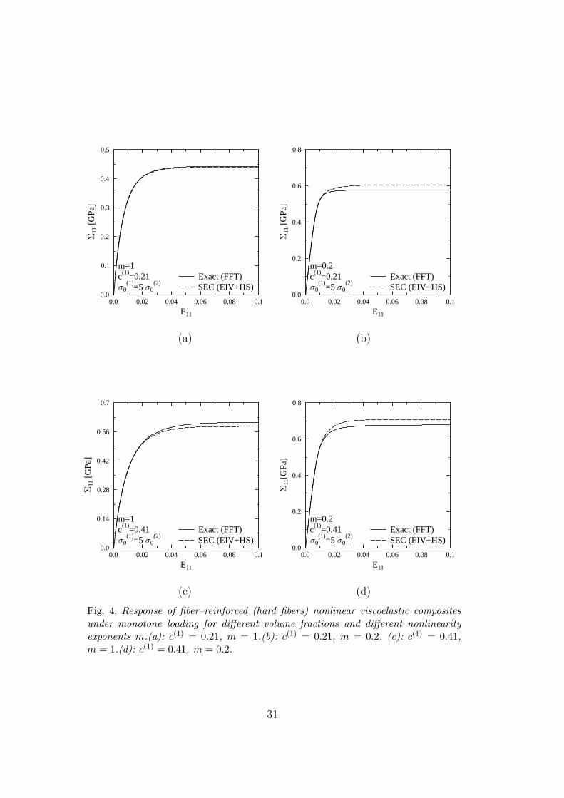
The responses of the two microstructures of figure 3 under monotone sheardeformation are shown in figures 4 and 5 where the overall stress is plotted asa function of the overall strain. The full-field simulations are shown as solidlines whereas the predictions of the present model are shown as dashed lines.

As in the three-dimensional case, the main trends of the stress-strain curvefor these composites under monotone deformation at constant strain-rate aretypically an initial linear-elastic response for incipient strains, then a transientpart and finally a plateau corresponding to the purely viscous response of thecomposite. This plateau is characterized by a stress Σ∞

11.

Figure 4 corresponds to the case of “hard” fibers (σ10/σ

20 = 5), whereas figure 5

corresponds to “weak” fibers (σ10/σ

20 = 0.2). In both figures two rate-sensitivity

exponents are considered, m = 1 (corresponding to linear viscoelasticity) andm = 0.2. The following comments can be made :

29

(1) In the linear case (m = 1) the error introduced by the model is essentiallydue to the HS bound. There is an additional error introduced by the EIVapproximation, when the heterogeneous field αn is replaced by a piecewiseuniform effective internal variable, but this additional error is small asalready seen in section 5.1.

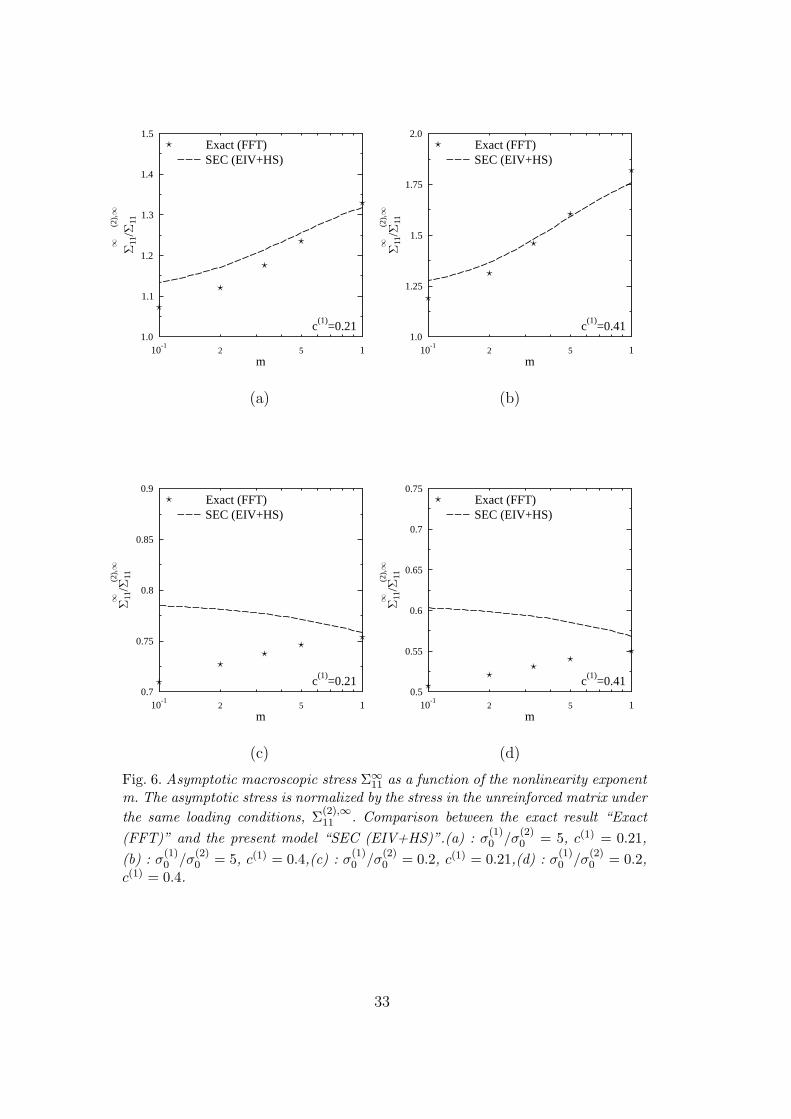
(2) In all cases the largest error is found in the asymptotic regime. It istherefore possible to better quantify the error introduced by the modelby comparing the asymptotic stresses Σ∞

11. This is done in figure 6 wherethe asymptotic stress is plotted as a function of the nonlinearity expo-nent. The accuracy of the model in the asymptotic regime is essentiallydictated by the choice of the linearization scheme for the dissipation po-tential ϕ and is not much influenced by the other approximations made bythe model (time-discretization, stationarity conditions, effective internalvariable).

(3) Regarding the linearization technique, it is now well-recognized that the“modified secant method” used here (which is a special case of the vari-ational procedure of Ponte Castaneda) has the advantage of simplicitybut can lead to significant errors for large contrast between the phasesor high volume fraction of the constituents. This is especially true forfiber-weakened composites as can be seen in figure 6c and d. The errorremains acceptable for fiber-reinforced composites, but is mainly due to a“compensation of errors” between the underestimation brought by the HSlower bound and the overestimation due to the linearization scheme itself(contained in inequality (42)). Improving on the “secant linearization” isthe objective of part II of this study (companion paper).

6 Conclusion

This paper is devoted to the effective response of composites, or more gen-erally of heterogeneous materials, whose individual constituents exhibit bothreversible and irreversible effects in their mechanical behavior. The main find-ings are:

(1) Upon time-discretization of the constitutive differential equations, an in-cremental variational principle has been derived, by means of which theproblem can be reduced to the minimization of a single nonquadraticincremental potential.

(2) The spatial dependence of the incremental potential stems not only fromthe variation of the potential from phase to phase, as is naturally the casein heterogeneous systems, but also from the dependence of this incremen-tal potential on the field of internal variables at the previous time-stepwhich is nonuniform even within each phase.

(3) A strategy, inspired by the variational procedure of Ponte Castaneda, has

30

0.0 0.02 0.04 0.06 0.08 0.1

E11

0.0

0.1

0.2

0.3

0.4

0.5

11[G

Pa]

Exact (FFT)SEC (EIV+HS)

m=1c

(1)=0.21

0(1)

=5 0(2)

(a)

0.0 0.02 0.04 0.06 0.08 0.1

E11

0.0

0.2

0.4

0.6

0.8

11[G

Pa]

Exact (FFT)SEC (EIV+HS)

m=0.2c

(1)=0.21

0(1)

=5 0(2)

(b)

0.0 0.02 0.04 0.06 0.08 0.1

E11

0.0

0.14

0.28

0.42

0.56

0.7

11[G

Pa]

Exact (FFT)SEC (EIV+HS)

m=1c

(1)=0.41

0(1)

=5 0(2)

(c)

0.0 0.02 0.04 0.06 0.08 0.1

E11

0.0

0.2

0.4

0.6

0.8

11[G

Pa]

Exact (FFT)SEC (EIV+HS)

m=0.2c

(1)=0.41

0(1)

=5 0(2)

(d)

Fig. 4. Response of fiber–reinforced (hard fibers) nonlinear viscoelastic compositesunder monotone loading for different volume fractions and different nonlinearityexponents m.(a): c(1) = 0.21, m = 1.(b): c(1) = 0.21, m = 0.2. (c): c(1) = 0.41,m = 1.(d): c(1) = 0.41, m = 0.2.

31

0.0 0.02 0.04 0.06 0.08 0.1

E11

0.0

0.1

0.2

0.3

11[G

Pa]

Exact (FFT)SEC (EIV+HS)

m=1c

(1)=0.21

0(1)

= 0(2)

/5

(a)

0.0 0.02 0.04 0.06 0.08 0.1

E11

0.0

0.1

0.2

0.3

0.4

0.5

11[G

Pa]

Exact (FFT)SEC (EIV+HS)

m=0.2c

(1)=0.21

0(1)

= 0(2)

/5

(b)

0.0 0.02 0.04 0.06 0.08 0.1

E11

0.0

0.04

0.08

0.12

0.16

0.2

11[G

Pa]

Exact (FFT)SEC (EIV+HS)

m=1c

(1)=0.41

0(1)

= 0(2)

/5

(c)

0.0 0.02 0.04 0.06 0.08 0.1

E11

0.0

0.1

0.2

0.3

0.4

11[G

Pa]

Exact (FFT)SEC (EIV+HS)

m=0.2c

(1)=0.41

0(1)

= 0(2)

/5

(d)

Fig. 5. Response of fiber–weakened (weak fibers) nonlinear viscoelastic compositesunder monotone loading for different volume fractions and different nonlinearityexponents m.(a): c(1) = 0.21, m = 1.(b): c(1) = 0.21, m = 0.2. (c): c(1) = 0.41,m = 1.(d): c(1) = 0.41, m = 0.2.

32

10-1

2 5 1m

1.0

1.1

1.2

1.3

1.4

1.511

/11

Exact (FFT)SEC (EIV+HS)

c(1)

=0.21

(2),

(a)

10-1

2 5 1m

1.0

1.25

1.5

1.75

2.0

11/

11

Exact (FFT)SEC (EIV+HS)

c(1)

=0.41

(2),

(b)

10-1

2 5 1m

0.7

0.75

0.8

0.85

0.9

11/

11

Exact (FFT)SEC (EIV+HS)

c(1)

=0.21

(2),

(c)

10-1

2 5 1m

0.5

0.55

0.6

0.65

0.7

0.75

11/

11

Exact (FFT)SEC (EIV+HS)

c(1)

=0.41

(2),

(d)

Fig. 6. Asymptotic macroscopic stress Σ∞11 as a function of the nonlinearity exponent

m. The asymptotic stress is normalized by the stress in the unreinforced matrix under

the same loading conditions, Σ(2),∞11 . Comparison between the exact result “Exact

(FFT)” and the present model “SEC (EIV+HS)”.(a) : σ(1)0 /σ

(2)0 = 5, c(1) = 0.21,

(b) : σ(1)0 /σ

(2)0 = 5, c(1) = 0.4,(c) : σ

(1)0 /σ

(2)0 = 0.2, c(1) = 0.21,(d) : σ

(1)0 /σ

(2)0 = 0.2,

c(1) = 0.4.

33

been used to linearize the nonquadratic condensed potential and also todefine an “effective internal variable” per phase at each time-step.

(4) Comparisons with full-field simulations show that the present model isgood as long as the variational procedure is accurate in the purely dis-sipative setting, when elastic deformations are neglected. If this is thecase, the present model accounts in a very satisfactory manner for thecoupling between reversible and irreversible effects and is therefore anaccurate model for treating nonlinear viscoelastic and elasto-viscoplasticmaterials.

(5) In certain situations, the variational procedure is not accurate in thepurely dissipative limit and examples of such situations are given. Theymotivate the second part of this study in which a more refined scheme,still based on the condensed variational potential derived in this first part,but with a different linearization strategy based on an anisotropic linearviscoelastic composite, is proposed.

Acknowledgements

This study is part of program supported by the Centre National de la RechercheScientifique under grant CNRS/NSF n◦14555. The authors thank R. Massonfor refreshing their mind about the work of Mialon (1986).

References

Bao, G., Hutchinson, J., McMeeking, R., 1991. Particle reinforcement of duc-tile matrices against plastic flow and creep. Acta Metall. Mater. 39, 1871–1882.

Bardella, L., 2003. An extension of the secant method for the homogenizationof the nonlinear behavior of composite materials. Int. J. Engng Sc. 41,741–768.

Berveiller, M., Zaoui, A., 1979. An extension of the self-consistent scheme toplastically-flowing polycrystals. J. Mech. Phys. Solids 26, 325–344.

Brenner, R., Masson, R., 2005. Improved affine estimates for nonlinear vis-coelastic composites. Eur. J. Mechanics A/Solids 24, 1002–1015.

Brenner, R., Masson, R., Castelnau, O., Zaoui, A., 2002. A ”quasi-elastic”affine formulation for the homogenised behaviour of nonlinear viscoelasticpolycrystals and composites. European Journal of Mechanics - A/Solids 21,943–960.

Buryachenko, V., 2001. Multiparticle effective field and related methods inmicromechanics of composite materials. Appl. Mech. Rev. 54, 1–47.

Chaboche, J., Kruch, S., Maire, J., Pottier, T., 2001. Towards a micromechan-

34

ics based inelastic and damage modeling of composites. Int. J. Plasticity 17,411–439.

Christman, T., Needleman, A., Suresh, S., 1989. An experimental and numer-ical study of deformation in metal-ceramic composites. Acta Metall. Mater.37, 3029–3050.

Chu, T., Hashin, Z., 1971. Plastic behavior of composites and porous mediaunder isotropic stress. Int. J. Engng Sci. 9, 971–994.

Dvorak, G., 1992. Transformation field analysis of inelastic composite materi-als. Proc. R. Soc. Lond. A 437, 311–327.

Dvorak, G., Bahei-El-Din, Y., Wafa, A., 1994. The modeling of inelastic com-posite materials with the transformation field analysis. Modelling Simul.Mater. Sci. Eng 2, 571–586.

Ekeland, I., Temam, R., 1976. Convex Analysis and Variational Problems.North-Holland, Amsterdam.

Fish, J., Shek, K., 1998. Computational plasticity and viscoplasticity for com-posite materials and structures. J. Composites 29B, 613–619.

Germain, P., Nguyen, Q., Suquet, P., 1983. Continuum Thermodynamics. J.Appl. Mech. 50, 1010–1020.

Gonzalez, C., Segurado, J., Llorca, J., 2004. Numerical simulation of elasto-plastic deformation of composites: evolution of stress microfields and impli-cations for homogenization models. J. Mech. Phys. Solids 52, 1573–1593.

Halphen, B., Nguyen, Q., 1975. Sur les materiaux standard generalises. J.Mecanique 14, 39–63.

Hashin, Z., 1970. Complex moduli of viscoelastic composites–I General theoryand application to particulate composites. Int. J. Solids Structures 6, 539–552.

Idiart, M., Moulinec, H., Ponte Castaneda, P., Suquet, P., 2006. Macroscopicbehavior and field fluctuations in viscoplastic composites: second-order es-timates versus full-field simulations. J. Mech. Phys. Solids 54 , 1029–1063.

Lahellec, N., Suquet, P., 2004. Nonlinear composites: a linearization procedure,exact to second-order in contrast and for which the strain-energy and theaffine formulations coincide. C. R. Mecanique 332, 693–700.

Lahellec, N., Suquet, P., 2006. Effective behavior of linear viscoelastic com-posites: a time-integration approach. Int. J. Solids Structures 44, 507-529.

Lambrecht, M., Miehe, C., Dettmar, J., 2003. Energy relaxation of non-convexincremental stress potentials in a strain-softening elastic-plastic bar. Int. J.Solids Struct. 40, 1369–1391.

Lemaitre, J., Chaboche, J., 1994. Mechanics of Solid Materials. CambridgeUniversity Press, Cambridge.

Levesque, M., Derrien, K., Mishnaevsky Jr., L., Baptiste, D. and Gilchrist,M. D., 2004. A micromechanical model for nonlinear viscoelastic particlereinforced polymeric composite materials- undamaged state. CompositesPart A: Applied Science and Manufacturing 35, 905 - 913.

Levin, V., 1967. Thermal expansion coefficients of heterogeneous materials.Mekh. Tverd. Tela 2, 83–94.

35

Li, G., Ponte Castaneda, P., 1993. The effect of particle shape and stiffness onthe constitutive behavior of metal-matrix composites. Int. J. Solids Struct.30, 3189–3209.

Li, J., Weng, G., 1997. A secant-viscosity approach to the time-dependentcreep of an elastic-viscoplastic composite. J. Mech. Phys. Solids 45, 1069–1083.

Marigo J.J., Mialon P., Michel J.C., Suquet P., 1987? Plasticite et ho-mogeneisation : un exemple de prevision des charges limites d’une structureperiodiquement heterogene. J. Mecanique Theorique et Appliquee 6, 47-75.

Masson, R., Zaoui, A., 1999. Self-consistent estimates for the rate-dependentelastoplastic behaviour of polycrystalline materials. J. Mech. Phys. Solids47, 1543–1568.

Mialon, P., 1986. Elements d’analyse et de resolution numerique des relationsde l’elasto-plasticite. EDF Bulletin de la Direction des Etudes et recherches.Serie C. Mathematiques, Informatique, N◦3, 57-89.

Miehe, C., 2002. Strain-driven homogenization of inelastic micro-structuresand composites based on an incremental variational formulation. Int. J.Numer. Meth. Engng 55, 1285-1322.

Miehe, C., Schotte, J., Lambrecht M., 2002. Homogenization of inelastic mate-rials at finite strains based on incremental variational principles. Applicationto the texture analysis of polycrystals. J. Mech. Phys. Solids 50, 2123-2167.

Moulinec, H., Suquet, P., 1994. A fast numerical method for computing thelinear and nonlinear properties of composites. C. R. Acad. Sc. Paris II 318,1417–1423.

Moulinec, H., Suquet, P., 1998. A numerical method for computing the over-all response of nonlinear composites with complex microstructure. Comp.Meth. Appl. Mech. Engng. 157, 69–94.

Moulinec, H., Suquet, P., 2003. Intraphase strain heterogeneity in nonlinearcomposites: a computational approach. Eur. J. Mech.: A/ Solids 22, 751–770.

Moulinec, H., Suquet, P., 2004. Homogenization for nonlinear composites inthe light of numerical simulation. In:P. Ponte Castaneda, Telega, J. (Eds.),Nonlinear Homogenization and Its Application to Composites, Polycrystalsand Smart Materials. NATO Sciences Series II, vol 170. Kluwer Acad. Pub.,pp. 193–223.

Olson, T., 1997. Bounding the effective yield behavior of mixtures. in GoldenK., Grimmett G., James R. and Milton G. (Eds) Mathematics of MultiscaleMaterials, IMA Lecture Notes 99, Springer-Verlag, New-York, pp. 219-228.

Ortiz, M., Repetto, E., 1999. Nonconvex energy minimization and dislocationstructures in ductile single crystals. J. Mech. Physics Solids 47, 397–462.

Ortiz, M., Stainier, L., 1999. The variational formulation of viscoplastic con-stitutive updates. Comput. Methods Appl. Mech. Engrg 171, 419–444.

Ponte Castaneda, P., 1992. New variational principles in plasticity and theirapplication to composite materials. J. Mech. Phys. Solids 40, 1757–1788.

Ponte Castaneda, P., 1996. Exact second-order estimates for the effective me-

36

chanical properties of nonlinear composite materials. J. Mech. Phys. Solids44, 827–862.

Ponte Castaneda, P., 2002. Second-order homogenization estimates for nonlin-ear composites incorporating field fluctuations. I - Theory. J. Mech. Phys.Solids 50, 737–757.

Ponte Castaneda, P., Suquet, P., 1998. Nonlinear composites. Adv. Appl.Mech. 34, 171–302.

Ponte Castaneda, P., Willis, J. R., 1999. Variational second-order estimatesfor nonlinear composites. Proc. R. Soc. London A 455, 1799–1811.

Powell, M.J.D., 1970. A hybrid method for nonlinear algebraic equation. In: P.Rabinowitz (Ed.), Numerical Methods for Nonlinear Algebraic Equations,Gordon and Breach Pub.

Rice, J., 1970. On the structure of stress-strain relations for time-dependentplastic deformation in metals. J. Appl. Mech. 37, 728–737.

Sanchez-Hubert, J., Sanchez-Palencia, E., 1978. Sur certains problemesphysiques d’homogeneisation donnant lieu a des phenomenes de relaxation.C.R. Acad. Sc. Paris Serie A 286, 903–906.

Simo, J., Hughes, T.J.R., 1998. Computational Inelasticity. Springer-Verlag.New-York. 1998.

Suquet, P., 1987. Elements of Homogenization for Inelastic Solid Mechanics.In: Sanchez-Palencia, E., Zaoui, A. (Eds.), Homogenization Techniques forComposite Media. Vol. 272 of Lecture Notes in Physics. Springer Verlag,New York, pp. 193–278.

Suquet, P., 1993. Overall potentials and extremal surfaces of power law orideally plastic materials. J. Mech. Phys. Solids 41, 981–1002.

Suquet, P., 1995. Overall properties of nonlinear composites : a modified secantmoduli theory and its link with Ponte Castaneda’s nonlinear variationalprocedure. C.R. Acad. Sc. Paris serie IIb 320, 563–571.

Suquet, P., 1997. Effective properties of nonlinear composites. In: Suquet,P. (Ed.), Continuum Micromechanics. Vol. 377 of CISM Lecture Notes.Springer Verlag, New York, pp. 197–264.

Talbot, D., Willis, J., 1985. Variational principles for inhomogeneous nonlinearmedia. IMA J. Appl. Math. 35, 39–54.

Willis, J., 1981. Variational and related methods for the overall properties ofcomposites. Adv. Appl. Mech. 21, 1–78.

Appendix A: Link with the Transformation Field Analysis (TFA)

In an attempt to approximate w∆ by a piecewise uniform potential, the trialfield α involved in the variational problem (16) can be chosen to be uniform

37

within each phase :

α(x, t) =N∑

r=1

α(r)(t)χ(r)(x). (56)

In particular :

αn(x) =N∑

r=1

α(r)n χ(r)(x), (57)

with a similar expression for αn+1 (for simplicity the index n+1 will be omittedin the sequel). The restriction brought by (56) on the choice of the trial fieldsα leads to an upper bound for w∆ and therefore to an upper bound for theeffective incremental potential J at each time step. The resulting predictionwill be stiffer than the actual response of the composite.

The stationarity conditions with respect to α(r) in the variational problem(16) read as :

⟨[∂w(r)

∂α(ε(x), α(r)) +

∂ϕ(r)

∂α

(α(r) − α(r)

n

∆t

)]χ(r)(x)

⟩= 0, (58)

while the conditions expressing the stationarity with respect to ε read as :

σ(x) =∂w(r)

∂ε(ε(x), α(r)) in phase r. (59)

It follows from (58) and from the fact that α(r) and α(r)n are independent of

x, that :

A(r) =

∂ϕ(r)

∂α

(α(r) − α(r)

n

∆t

)= −

⟨∂w(r)

∂α(ε(x), α(r))

⟩

r

.

As a consequence of assumption (H2), σ is a linear function of ε and α withuniform moduli in phase r. Therefore, the average stress σ(r) over phase r isrelated to the average strain ε(r) and to α(r) by the same relation. The final setof evolution equations for the model obtained under the specific assumption(56) reads as :

σ(r) =∂w(r)

∂ε(ε(r), α(r)), A

(r) = −∂w(r)

∂α(ε(r), α(r)). (60)

A(r) =

∂ϕ(r)

∂α(α(r)), or equivalently α(r) =

∂ϕ(r)∗

∂A(A(r)), (61)

This is exactly the set of equations used in the TFA.

38

Appendix B: Effective thermoelastic energy for N-phase and two-phase composites

Consider a N -phase thermoelastic composite whose phase r is characterizedby the energy

w(r)(ε) =1

2ε : L

(r) : ε + ρ(r) : ε + f (r).

Its effective energy reads (Willis, 1981) :

w (E) =1

2E : L : E + ρ : E + f , (62)

where :

L = 〈L〉 +N−1∑

r=1

c(r)(L

(r) − L(N))

:(A(r) − I

), (63)

ρ = 〈ρ〉 +N−1∑

r=1

c(r)(A(r) − I

)T:(ρ(r) − ρ(N)

), (64)

f = 〈f〉 +N−1∑

r=1

c(r)(ρ(r) − ρ(N)

): a(r). (65)

These expressions simplify further for two-phase composites (N = 2). Ac-cording to Levin’s relations (Levin, 1967), the localization operators can beexplicitly expressed in terms of the effective stiffness L of the composite:

A(1) = I +1

c(1)

(L

(1) − L(2))−T

:(L − 〈L〉

)T, (66)

a(1) =1

c(1)

(L

(1) − L(2))−1

:(L − 〈L〉

):(L

(1) − L(2))−1

:(ρ(1) − ρ(2)

). (67)

It follows from these relations that the effective thermoelastic energy of thecomposite can be expressed in terms of the effective stiffness of the compositeonly :

w(E) = 〈f〉 + 〈ρ〉 : E + 12E : 〈L〉 : E

+12

[E + (∆L)−1 : ∆ρ

]:(L − 〈L〉

):[E + (∆L)−1 ∆ρ

],

(68)

where

∆L = L(1) − L

(2), ∆ρ = ρ(1) − ρ(2).

39

Appendix C: First and second moments of the strain field in a ther-moelastic composite

The first moments of the strain field ε in each phase of a linear thermoelasticcomposite can be expressed as (see for instance Willis, 1981) :

〈ε〉r = A(r) : E + a(r). (69)

A(r) is the strain localization tensor giving the average strain in phase r dueto the macroscopic strain E in the absence of thermal stresses (ρ(r) = 0).Similarly, a(r) is the average strain in phase r due to the thermal stresses(E = 0). Both tensors depend on the elastic moduli of the phases and onthe microstructure of the composite. Explicit expressions corresponding tospecific microstructures can be found in the literature. These tensors can alsobe evaluated numerically.

The second moment of the strain field is obtained by derivation of the effectiveenergy of the composite with respect to the elastic moduli L

(r) of the individ-ual phases (see for instance Ponte Castaneda and Suquet, 1998, Buryachenko,2001 or Ponte Castaneda, 2002) :

〈ε ⊗ ε〉r =2

c(r)

∂w0

∂L(r)

(70)

Detailed expressions for the effective energy in two-phase composites are givenin appendix B.

40