OPTIMAL DESIGN OF STRUCTURES WITH KINEMATIC NONLINEAR BEHAVIOR

By S. Pezeshk,1 Associate Member, ASCE

ABSTRACT: This paper suggests an optimization-based methodology for the design of minimum weight structures with kinematic nonlinear behavior. Attention is focused on three-dimensional reticulated structures idealized with beam elements under proportional static loadings. The algorithm used for optimization is based on a classical optimality criterion approach using an active-set strategy for extreme limit constraints on the design variables. A first-order necessary condition is derived and used as the basis of a fixed-point iteration method to search for the optimal design. A fixed-point iteration algorithm is used based on the criterion that at optimum design the nonlinear strain energy is equal in all members. A nonlinear analysis procedure for three-dimensional structures is discussed and used in de­veloping the optimization algorithm. Several examples are given to evaluate the validity of the underlying assumptions and to demonstrate some of the character­istics of the proposed procedures. The procedure is verified using two well-known examples.

INTRODUCTION

The minimum weight design of structures subjected to a stability con­straint is one of the most important problems in structural optimization, and it has attracted a great deal of interest in the structural mechanics community. Methods for optimum structural design have progressed rapidly in recent years. In particular, optimality criterion procedures have signifi­cantly advanced the minimum weight design of structures involving large finite element assemblies.

Linear Stability Constraint For most optimization procedures for stability problems, the constraints

are defined by the associated linear buckling eigenvalue problem. One prob­lem with optimizing structures with constraints on linear stability is that the optimum structure can have more than one critical eigenmode. Experience in recent years has revealed that generating multimodality by optimization with respect to eigenvalues is not uncommon (Olhoff and Taylor 1983; Szyszkowski 1990; Hjelmstad and Pezeshk 1991). In general, a structure with multiple eigenmodes tends to become sensitive to imperfection, and small deviations in the geometry of the structure can greatly reduce its load-carrying capacity. In general, whether multiple eigenmodes reduce a struc­ture's load-carrying capacity depends on the type and distribution of loading and the geometry of the structure. Khot (1981) overcame simultaneous mode designs by assigning specific interval separation to critical eigenvalues of truss-like structures.

Nonlinear Stability Constraint Quite frequently, studies in the literature reveal that a linearized stability

approach is used beyond its limits of applicability. Linear stability can only

'Asst. Prof., Dept. of Civ. Engrg., Memphis State Univ., Memphis, TN 38152. Note. Discussion open until September 1, 1992, To extend the closing date one

month, a written request must be filed with the ASCE Manager of Journals. The manuscript for this paper was submitted for review and possible publication on January 2, 1991. This paper is part of the Journal of Engineering Mechanics, Vol. 118, No. 4, April, 1992. ©ASCE, ISSN 0733-9399/92/0004-0702/$ 1.00 + $.15 per page. Paper No. 1125.

702

J. Eng. Mech. 1992.118:702-720.

Dow

nloa

ded

from

asc

elib

rary

.org

by

Uni

vers

ity o

f M

emph

is o

n 02

/08/

13. C

opyr

ight

ASC

E. F

or p

erso

nal u

se o

nly;

all

righ

ts r

eser

ved.

give physically significant answers if the linear analysis gives deformations that are exactly the same when geometric nonlinearity is considered. This only happens in a very few practical situations, such as a perfectly straight column under an axial load. In real engineering situations where the qual­itative nature of the behavior is completely unknown, linearized stability represented by critical eigenmodes does not provide an adequate represen­tation of nonlinear behavior of a structure. For such cases, it is more ap­propriate to optimize a structure on the basis of a nonlinear stability con­straint when the structure has an inherent tendency to possess nonlinear behavior.

Khot and Kamat (1983) were among the first researchers to develop an optimization method based on an optimality criterion to minimize the design weight under system nonlinear stability for truss structures. Later, Kamat and Ruangsilasingha (1985) and Kamat (1987) formulated stability in its nonlinear form. They solved two special cases. They addressed the problem of maximizing the critical load of shallow-space trusses and shallow-truss arches of a given configuration and volume.

Wu and Arora (1988) presented a design sensitivity analysis of the critical load for nonlinear structural systems by taking derivatives of discretized matrix equations with respect to design variables. They introduced three approaches using analysis information at the critical limit point. However, the first two approaches were abandoned because of some difficulties in numerical implementation. In the third approach, design sensitivity formulas were derived without using derivatives of displacements at the critical limit point. Wu and Arora (1988) implemented their method by using only truss structural components, since many impractical computations are required for other types of structures.

Levy and Perng (1988) discussed the optimal truss design to withstand nonlinear stability requirements. They developed a two-phase iterative pro­cedure of analysis and design. Phase one used analysis to determine insta­bility, and phase two used a recurrence relation based on optimality criteria for redesign.

Most recently, Park and Choi (1990) developed a continuum mechanics formulation of sizing design sensitivity analysis of the critical load factor for nonlinear structural systems. They applied their method to both truss and two-dimensional structures composed of beam elements. The proposed ap­proach by Park and Choi (1990) works at any prebuckling equilibrium con­figuration and yields accurate design sensitivity of the critical load; however, they found that the design sensitivity of the estimated critical load does not approach that of the actual critical load.

Virtually all of the methods developed in the area of linear and specially nonlinear stability optimal-design procedures have dealt with the optimi­zation of truss elements or truss-like idealized elements, but they are seldom engaged with complex stiffness elements such as three-dimensional beam elements. The present procedure develops an optimality criterion approach to determine the optimal minimum weight design of a structure idealized by three-dimensional beam elements with constraint on the nonlinear strain energy density distribution. This paper is an extension of previous work, especially that of Khot and Kamat (1983).

In the following sections, first the formulation of a nonlinear analysis procedure for three-dimensional structures will be discussed, then the prob­lem will be formally stated as a nonlinear stability constraint optimization with a single equality constraint. The description and formulation of the

703

J. Eng. Mech. 1992.118:702-720.

Dow

nloa

ded

from

asc

elib

rary

.org

by

Uni

vers

ity o

f M

emph

is o

n 02

/08/

13. C

opyr

ight

ASC

E. F

or p

erso

nal u

se o

nly;

all

righ

ts r

eser

ved.

nonlinear analysis procedure is a necessary step to create a foundation on which to build the optimization algorithm. The first-order necessary con­ditions will be derived and used as the basis of a fixed-point iteration method to search for the optimal design. The method is illustrated by examples of two- and three-dimensional structures.

NONLINEAR ANALYSIS

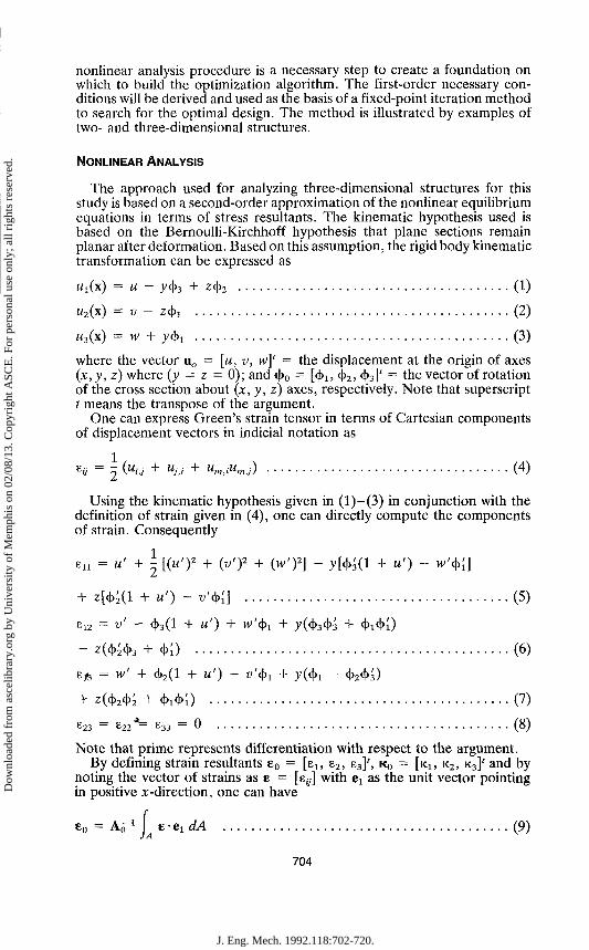
The approach used for analyzing three-dimensional structures for this study is based on a second-order approximation of the nonlinear equilibrium equations in terms of stress resultants. The kinematic hypothesis used is based on the Bernoulli-Kirchhoff hypothesis that plane sections remain planar after deformation. Based on this assumption, the rigid body kinematic transformation can be expressed as

Wi(x) = u - y4>3 + z<$>2 (1)

«2(x) = v ~ z4>i (2)

w3(x) = w + y$i (3)

where the vector u0 = [u, v, w]' = the displacement at the origin of axes (x, y, z) where (y = z = 0); and 4>0 = [(jh, (j>2, 4>3]' = the vector of rotation of the cross section about (x,y, z) axes, respectively. Note that superscript t means the transpose of the argument.

One can express Green's strain tensor in terms of Cartesian components of displacement vectors in indicial notation as

BU = 2 ("'V + "/.<• + Um,iUm,,) (4)

Using the kinematic hypothesis given in (l)-(3) in conjunction with the definition of strain given in (4), one can directly compute the components of strain. Consequently

en = W + \ [(u'f + (v'f + (w'f] - y[^(l + u') - w'fo]

+ z[c|>;(l + «') - v'fo] (5)

El2 = V' - <t>3(l + U') + W'fa + y(4>3<t>3 + * l4>0

- z(<|>2<j>3 + 4,0 (6)

EJ3 = W' + 4>2(1 + « ' ) - W'4>! + V(4>i - <\>2<^>3)

+ zfafo + t^cK) (7)

e23 = ^22 = e33 = 0 (°)

Note that prime represents differentiation with respect to the argument. By defining strain resultants e0 = [e1; e2, e3]', KQ = [KI, K2, K3]' and by

noting the vector of strains as e = [e:>] with ex as the unit vector pointing in positive x-direction, one can have

e0 = A6"1 JA e-ej dA (9)

704

J. Eng. Mech. 1992.118:702-720.

Dow

nloa

ded

from

asc

elib

rary

.org

by

Uni

vers

ity o

f M

emph

is o

n 02

/08/

13. C

opyr

ight

ASC

E. F

or p

erso

nal u

se o

nly;

all

righ

ts r

eser

ved.

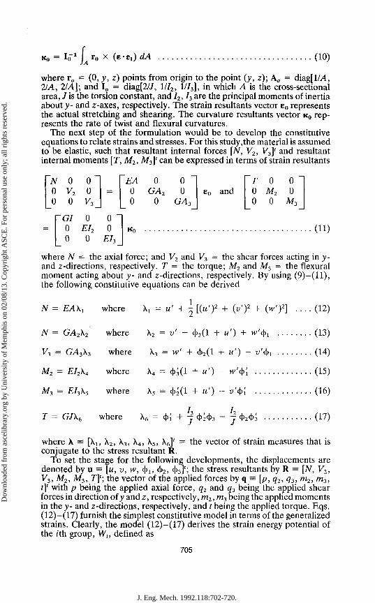
Ko = Io_1 \A*o x (e-ex) dA (10)

where r0 = (0, y, z) points from origin to the point (y, z); A0 = diag[lM, 21 A, 2/A]; and I? = diag[2/7, IIIz, 1/I3], in which A is the cross-sectional area, J is the torsion constant, and I2,I3 are the principal moments of inertia about y- and z-axes, respectively. The strain resultants vector e0 represents the actual stretching and shearing. The curvature resultants vector KQ rep­resents the rate of twist and flexural curvatures.

The next step of the formulation would be to develop the constitutive equations to relate strains and stresses. For this study,the material is assumed to be elastic, such that resultant internal forces [N, V2, V3]' and resultant internal moments [T, M2, M3]' can be expressed in terms of strain resultants

0 v2 0

GI 0 0

0 0 v3_

=

0 0 1 EI2 0 0 Eh

EA 0 0

0 GA2

0

0 0

GA3

and T O O 0 M2 0 0 0 M3

Ko (11)

where N = the axial force; and V2 and V3 = the shear forces acting in y-and z-directions, respectively. T = the torque; M2 and M3 = the flexural moment acting about y- and z-directions, respectively. By using (9)—(11), the following constitutive equations can be derived

\x = u' + \ [(w')2 + K ) 2 + {">'?} •••• (12)

X2 = v' - <t>3(l + u') + w'fyi (13)

K3 = w' + <j>2(l + «') - i/<t>! (14)

\4 = ct>3(l + u') - w'$[ (15)

X5 = 4.2(1 + u') - y'4>I (16)

h , I2

K = <K + J 4>2<t>3 ~ J 4>2<}>3 (17)

N = EA\X

N = GA2\2

V3 = GA3\3

M2 = EI2\4

M3 = EI3k5

T = GJK

where

where

where

where

where

where

where X = [\lt \2, \3 k6]' — the vector of strain measures that is conjugate to the stress resultant R.

To set the stage for the following developments, the displacements are denoted by u = [u, v, w, fa, fa, fa)'; the stress resultants by R = [N, V2, V3, M2, M3, T]1; the vector of the applied forces by q = [p,q2,q3,m2,m3, t]' with p being the applied axial force, q2 and q3 being the applied shear forces in direction ofy and z, respectively, m2, m3 being the applied moments in the y- and z-directions, respectively, and t being the applied torque. Eqs. (12)-(17) furnish the simplest constitutive model in terms of the generalized strains. Clearly, the model (12)-(17) derives the strain energy potential of the z'th group, W,, defined as

705

J. Eng. Mech. 1992.118:702-720.

Dow

nloa

ded

from

asc

elib

rary

.org

by

Uni

vers

ity o

f M

emph

is o

n 02

/08/

13. C

opyr

ight

ASC

E. F

or p

erso

nal u

se o

nly;

all

righ

ts r

eser

ved.

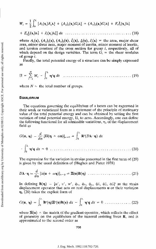
w> = \ f t ^ ' W £ A ! + 042),-(x,)G,-X! + (^3),(x,)G,.x§ + £,/,(x,)\

+ E,/,(x,>§ + 7/(s,)X§] dx (18)

where At(x), (^42),(x), (v43),(x), /,(x), 7,(x)> -Mx) = the area, major shear area, minor shear area, major moment of inertia, minor moment of inertia, and torsion constant of the cross section for group i, respectively, all of which depend on the design variables. The term G, = the shear modulus of group /.

Finally, the total potential energy of a structure can be simply expressed as

n = 2 W,, - \\'q ds (19) 1 = 1 JO

where N = the total number of groups.

EQUILIBRIUM

The equations governing the equilibrium of a beam can be expressed in their weak or variational form as a statement of the principle of stationary value of the total potential energy and can be obtained by setting the first variation of total potential energy, II, to zero. Accordingly, one can define the following functional for all admissible variations, T|, of the displacement field as

G(u, -n) = ~ [II(*i + au)] a = 0 = £ R'(Z)X--n) dx

L

tl'q dx = 0 (20)

The expression for the variation in strains presented in the first term of (20) is given by the usual definition of (Hughes and Pister 1978)

D\v) ^ £ [\(u + anOUo - H(u)B(m) (21)

In defining B(in) = [u', v', w', 4>1; ct>2, <J>3, 4>i, cbi, §3]' as the strain displacement operator that acts on real displacements u or their variation r\, (20) takes the explicit form of

G(u, i)) = ) B'(Y))3'(U)R(X) dx - Jo ti'q dx = 0 (22)

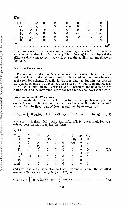
where S(u) = the matrix of the gradient operator, which reflects the effect of geometry on the equilibrium of the internal resisting force R, and is approximated to the second order as

706

J. Eng. Mech. 1992.118:702-720.

Dow

nloa

ded

from

asc

elib

rary

.org

by

Uni

vers

ity o

f M

emph

is o

n 02

/08/

13. C

opyr

ight

ASC

E. F

or p

erso

nal u

se o

nly;

all

righ

ts r

eser

ved.

g(u) =

1 + u' — 4»3

(f)2 fy'i 4>2 0

1—

v' w' 1 ch

-4>i i o <h

- < h o 0 0

0 — w' -v' 0 0 0

0 0

1 + u' 0 0 0

1 0

+ u' 0 0 0 0

0 0 0

-w' — v'

1 1

0 0 0 0

+ u' 0

0 0 0

1 + u' 0 0

( (23)

Equilibrium is satisfied for any configuration, u, in which G(u, r\) = 0 for any admissible virtual displacement -q. Thus, G(u, i\) has the physical sig­nificance that it measures, in a weak sense, the equilibrium imbalance in the system.

SOLUTION PROCEDURE

The system's motion involves geometric nonlinearity. Hence, the pro­cedure of linearization about an intermediate configuration must be used in the solution scheme. Specific details regarding the linearization process are treated extensively by Hughes and Pister (1978), Marsden and Hughes (1983), and Hjelmstad and Pezeshk (1988). Therefore, the final results are stated here, and the interested reader can refer to the cited works for details.

Linearization of the Weak Form By using standard procedures, the weak form of the equilibrium equations

can be linearized about an intermediate configuration u, with incremental motion Au. The linear part of G(u, t)) can then be expressed as

L(G)a = / ; B'(ri)[Ag(R) + H'(u)D(x)S(u)]B(Au) dx + G(u, •*]) . . (24)

where D = diag[EA, GA2, GA3, EI2, EI3, GJ]; for the formulation con­sidered here the matrix Ag has the form

A*(R) =

N 0 0 0 v,

-v? 0

M, M-,

0 TV 0

- v , 0 0

- M 3

0 0

0 0 N v? 0 0

-M2

0 0

0 -v, v, 0 0 0 0 0 0

v, 0 0 0 0 0 0 0 0

-v? 0 0 0 0 0 0 0 0

0 - M , - M 2

0 0 0 0 0 0

Af, 0 0 0 0 0 0 0 0

M7 0 0 0 0 0 0 0 0

(25)

and gives rise to the geometric part of the stiffness matrix. The so-called residual G(u, *i) is given by (21) and (22) as

G(u, *i) = B'(Tf))S'(u)R dx / > rq dx. (26)

707

J. Eng. Mech. 1992.118:702-720.

Dow

nloa

ded

from

asc

elib

rary

.org

by

Uni

vers

ity o

f M

emph

is o

n 02

/08/

13. C

opyr

ight

ASC

E. F

or p

erso

nal u

se o

nly;

all

righ

ts r

eser

ved.

NONLINEAR ANALYSIS OF STRUCTURES

The equations for equilibrium can be discretized by using the finite ele­ment method and can be solved by using an incremental procedure with a Newton-Raphson iteration at each step. Ramm (1980) has presented a gen­eral summary of algorithms for tracing the response of a structure, including passage through limit-load points. A displacement control procedure was used to analyze the problems (Ramm 1980).

FORMULATION AND DEVELOPMENT OF OPTIMIZATION PROBLEM

Nonlinear critical load, which may be either a limit or a bifurcation point, can be characterized as the load that results in a loss of positive definiteness of the tangent stiffness matrix. For the optimization problem considered here, the load distribution applied to the structure is specified and is assumed to be proportional. The structure's geometry is given, and the optimization problem seeks to procure the minimum weight design of a structure, such that for the given design load distribution an instability can be achieved. The instability can be a limit or a bifurcation point. The structure is idealized with nonlinear beam elements and, in each optimization cycle, the structure is analyzed using the geometrically nonlinear procedure formulated earlier. By using a displacement control procedure such as Ramm (1980) and Batoz and Dhatt (1979), one can reach and pass a limit or a bifurcation point. A limit or a bifurcation point can be traced either by monitoring the positive definiteness of the tangent stiffness matrix or using the current stiffness parameter developed by Bergan and Soreide (1978). They showed that the nonlinear behavior of multidimensional problems may be characterized by a single scalar quantity called the current stiffness parameter. The current stiffness parameter is implemented and used in this study. As soon as the load approaches instability, the current stiffness parameter approaches zero and becomes zero right at the instability load, changing its sign after passing the instability point.

For the present study, the members of the structures are arranged into M distinct groups. Each group is associated with a set of design variables that describe the geometry of the cross section of that group. For example, an I-beam can be described by its depth h, flange width b, web thickness t, and flange thickness tf. Consequently, the I-beam has four design varia­bles. A rectangular cross section has two design variables, the width b and the height h. A square cross section can be identified by one design variable, which can be either the width or the height. The vector of design variables will be designated as x = {xl7 x2, . . . , xdv], where dv is the number of design variables, computed as the sum over all the groups of the number of design variables per group. Therefore, the optimization algorithm can handle complex cross sections with several variables to describe the cross section. One important point is that this study is not concerned with local buckling, but with global instability of a structure. Because the analytical model does not include local buckling modes, these will not be represented in the objective function or constraint functions. One could use a model that incorporates local buckling, but the interaction between local and global buckling is small for most structures. However, since local and global buck­ling are lightly coupled, local buckling constraints in the form of width-to-thickness limitation would be relatively simple to describe and implement.

To simplify notation, the specific weight of the mth group is designated as the weight per unit of the cross-sectional area of the entire group

708

J. Eng. Mech. 1992.118:702-720.

Dow

nloa

ded

from

asc

elib

rary

.org

by

Uni

vers

ity o

f M

emph

is o

n 02

/08/

13. C

opyr

ight

ASC

E. F

or p

erso

nal u

se o

nly;

all

righ

ts r

eser

ved.

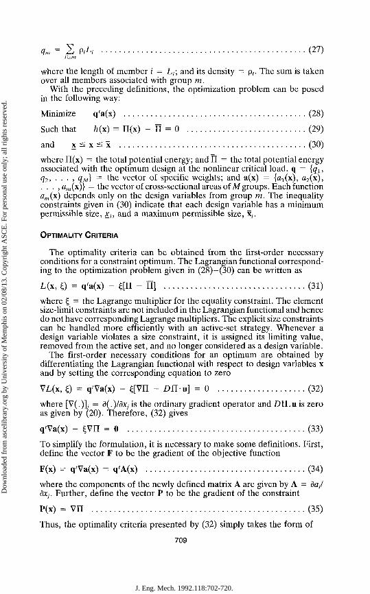
qm = 2 P/A (27)

where the length of member i = L,; and its density = p,. The sum is taken over all members associated with group m.

With the preceding definitions, the optimization problem can be posed in the following way:

Minimize q'a(x) (28)

Such that h(x) = II(x) - TT = 0 (29)

and x < x < x (30)

where II(x) = the total potential energy; and II = the total potential energy associated with the optimum design at the nonlinear critical load, q = {q±, #2; • • • > QM) — t n e vector of specific weights; and a(x) = {fli(x), a2(x), . . . ,am(x)} = the vector of cross-sectional areas of M groups. Each function am(x) depends only on the design variables from group m. The inequality constraints given in (30) indicate that each design variable has a minimum permissible size, x,, and a maximum permissible size, x,.

OPTIMALITY CRITERIA

The optimality criteria can be obtained from the first-order necessary conditions for a constraint optimum. The Lagrangian functional correspond­ing to the optimization problem given in (28)-(30) can be written as

L(x, 0 = q'a(x) - £[II - II] (31)

where £ = the Lagrange multiplier for the equality constraint. The element size-limit constraints are not included in the Lagrangian functional and hence do not have corresponding Lagrange multipliers. The explicit size constraints can be handled more efficiently with an active-set strategy. Whenever a design variable violates a size constraint, it is assigned its limiting value, removed from the active set, and no longer considered as a design variable.

The first-order necessary conditions for an optimum are obtained by differentiating the Lagrangian functional with respect to design variables x and by setting the corresponding equation to zero

VL(x, 0 = q'Va(x) - £[VII - DUu] = 0 (32)

where [V(.)]; = 3(.)/dx, is the ordinary gradient operator and DII.u is zero as given by (20). Therefore, (32) gives

q'Va(x) - £Vn = o (33)

To simplify the formulation, it is necessary to make some definitions. First, define the vector F to be the gradient of the objective function

F(x) = q'Va(x) = q'A(x) (34)

where the components of the newly defined matrix A are given by A = datl dXj. Further, define the vector P to be the gradient of the constraint

P(x) = Vn (35)

Thus, the optimality criteria presented by (32) simply takes the form of

709

J. Eng. Mech. 1992.118:702-720.

Dow

nloa

ded

from

asc

elib

rary

.org

by

Uni

vers

ity o

f M

emph

is o

n 02

/08/

13. C

opyr

ight

ASC

E. F

or p

erso

nal u

se o

nly;

all

righ

ts r

eser

ved.

F(x) - £P(x) = 0 (36)

This equation geometrically signifies that, to have an optimal solution for a design x, the vectors F and P must be collinear.

Later, the derived optimality criteria, (36), will be used to set up the recurrence algorithm for updating the design vector x. To simplify the no­tation for future developments, one can define a diagonal quotient matrix Q such that

G'/ = §; if i = i (37fl) &y = 0 if i+j (37b)

Therefore, by using the definition given in (31 a,b) and by considering the optimally criteria given in (36), one will arrive at the following simplified optimality criteria expression

Q(x) = 1 (38)

where I is the identity matrix.

SOLUTION PROCEDURE

The optimum design must satisfy the optimality criteria and the nonlinear energy density constraint. Since these equations are nonlinear, they must be solved by an iterative procedure. The algorithm used here is a fixed-point iteration based on the first-order necessary conditions (optimality criteria). The fixed-point iteration, used in conjunction with a scaling pro­cedure, will move the initial design toward a configuration that satisfies the optimality criteria and the constraints. The algorithm steps are as follows:

1. Choose an initial design. 2. Perform a nonlinear analysis and determine the nonlinear limit load. 3. Perform a line search (scaling) to satisfy the constraint, and keep the design

in feasible region by assuming the Lagrange multiplier is equal to one. 4. Select a design vector direction and determine new design variables. 5. Check the optimality criteria. 6. If convergence is not achieved, go to step 2.

The Fixed-Point Iteration Various forms of recurrence relations have been developed by researchers

and have been used to update the configuration in an optimization problem (Gellaty and Berke 1971; Khot et al. 1976). The recursive approach has the advantage in that it eliminates the need for the Hessian of the Lagrangian functional required in a nonlinear programming algorithm. In general, the optimality criteria are used to modify the design variable vector. Therefore, one can generate a new design vector from the previous one with the ex­ponential recursion relation

X K+I = XKrQ(XK-, j ( i f r ) ( 3 9 )

where K denotes the iteration number and r is the step size parameter. At the optimum, the optimality criteria will be satisfied; therefore, the design variables will be unchanged with any additional iterations at optimum. The

710

J. Eng. Mech. 1992.118:702-720.

Dow

nloa

ded

from

asc

elib

rary

.org

by

Uni

vers

ity o

f M

emph

is o

n 02

/08/

13. C

opyr

ight

ASC

E. F

or p

erso

nal u

se o

nly;

all

righ

ts r

eser

ved.

convergence behavior depends on the parameter r. Depending on the be­havior of the constraint, it may be necessary to increase r to prevent con­vergence.

At the optimum, the term Q(xK) given in (30) approaches identity. There­fore, linearizing the exponential gives the alternate recurrence relation

XK+I = X K | I + I [ Q ( X K ) _ !]l (40)

This equation is referred to as the linear recurrence relation for the design variables and can be used to update the design.

Scaling Procedure After each iteration, the design variables must be scaled to ensure that

the specified load on the structure is equal to the nonlinear critical load of the structure. The problem of scaling is essentially a line search in the direction of the current design vector x. One wishes to make the limit load or the bifurcation instability load to be the actual load applied for the scaled design variables £x, where the following notation has been proposed to accommodate the active-set strategy:

l> i _ Cx/ f° r ' m t n e active set ,.^ *• x,- for / not in the active set *• '

The following is a development of the scaling procedure for square mem­bers. The scaling procedure is based on scaling the moment of inertia of the members. To present the method in its simplest form, the method is confined to one-design-variable sections. The same procedure can be de­veloped for I-beam and rectangular cross sections.

The moment of inertia of each member of the structure after each iteration can be divided into two groups, depending on whether design variables are active or passive. Thus, the vector of the moment of inertias as a function of design variable vector x is given by

T = I"(x) + IP(X) (42)

where T = scalar measure of total moment of inertias of the structure. A superscript a indicates an active design variable, and a superscript p indicates a passive design variable. /" is the summation of all active moment of inertias of the structure, and Ip is the summation of all the passive moment of inertias of the structure.

The proportional load distribution applied to the structure can be rep­resented by X, which = a load factor, times the actual loading, applied to the structure. After each iteration, the load factor X is determined from the nonlinear analysis of the structure. Then the structure is scaled to ensure that the specified load on the structure is equal to the nonlinear critical load of the structure. All the design variables are scaled by the same factor. Performing such scaling procedure is based on the important assumption that the nonlinear deformation or the nonlinear buckling response of the structure at limit load is basically the same as the scaled structure with all of its moment of inertias scaled uniformly.

The scaling factor, £, will force the structure to have a unity for the load factor, X = 1, after each iteration. Solving for the scaling factor from (42) gives

711

J. Eng. Mech. 1992.118:702-720.

Dow

nloa

ded

from

asc

elib

rary

.org

by

Uni

vers

ity o

f M

emph

is o

n 02

/08/

13. C

opyr

ight

ASC

E. F

or p

erso

nal u

se o

nly;

all

righ

ts r

eser

ved.

l=f^ (43) All of the design variables will be scaled by the scaling factor £ determined in (43), and all the cross-sectional properties will be determined from the scaled design variables accordingly.

Active-Set Constraint Strategy After each iteration, a new set of design variables is obtained. If a design

variable lies within its permissible range, it is placed in the active set; other­wise, it is placed in the passive set so that a proper scaling can be performed before the next iteration. At the start of each iteration, a formerly passive variable can either remain in the passive set or be reactivated. In general, it is not known a priori if a variable will be active at the optimum.

Sensitivity Analysis Evaluation of the optimality conditions (36), requires knowledge of the

sensitivity, or rate of change, of the potential energy with respect to the design variables. The sensitivity of the potential energy can be computed by differentiating the potential energy given in (19) with respect to design variable x

VII = VW (44)

in which the differentiation of the strain energy involves only differentiation of the scalar cross-sectional parameters of (18)

VW,- = \ ^ [VA^EM + V(A2)i(xi)Gl\l + V(^3),(x,)G,X§

+ V/,.£,(x,)^4 + V/,.£,.(x,)M + V7,(x,)^6] dx - JQ VVq dx (45)

where I = [Ilt I2, . . . , Im]' = the vector of major moment of inertias of M groups; I = [[1; I2, . . . , [„]' - the vector of minor moment of inertias of M group; J = [J1, J2, . . . , Jm]' = the vector of torsion constants of M groups. Each function, such as ^ ( x ) , depends only on the design variables from group m. The sensitivities of X, are identically zero for statically de­terminate structures since the distribution of force through the structure does not depend on the element rigidities. In addition, such sensitivities are usually small and are generally neglected in practical computations for in­determinate structures.

The following section describes how the developed nonlinear analysis procedure and the proposed optimization method are applied to several simple structures. The purpose of the examples is to demonstrate how the algorithm performs.

EXAMPLES

In all the example problems investigated in this report, Young's modulus of elasticity of 107 psi and material density, p, of the 0.1 lb per cubic in. were used. A square cross section was used for all the members with a minimum allowable size of 0.316 in. for each design variable (or 0.1 sq. in. for minimum allowable cross-sectional area). Each design variable consists

712

J. Eng. Mech. 1992.118:702-720.

Dow

nloa

ded

from

asc

elib

rary

.org

by

Uni

vers

ity o

f M

emph

is o

n 02

/08/

13. C

opyr

ight

ASC

E. F

or p

erso

nal u

se o

nly;

all

righ

ts r

eser

ved.

of either height or width of a square cross section. In addition, each structural member is modeled with two three-noded quadratic geometrically nonlinear beam elements.

The analysis and the optimization procedure, used to analyze and design the structures studied here, are implemented in the general finite element program FEAP (Zienkiewicz 1982).

TWO-BAR ASYMMETRICAL TRUSS STRUCTURE

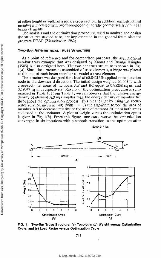
As a point of reference and for comparison purposes, the asymmetrical two-bar truss example that was designed by Kamat and Ruangsilasingha (1985) is also designed here. The two-bar truss structure is shown in Fig. 1(a). Since the structure is assembled of truss elements, a hinge was placed at the end of each beam member to model a truss element.

The structure was designed for a load of 60.04215 lb applied at the junction node in the downward direction. The initial design weighed 20.003 lb with cross-sectional areas of members AB and BC equal to 0.95238 sq in. and 0.19047 sq in., respectively. Results of the optimization procedure is sum­marized in Table 1. From Table 1, we can observe that the relative energy density of element AB was smaller than the energy density of member BC throughout the optimization process. This meant that by using the recur­rence relation given in (40) (with r = 6) the algorithm forced the area of member AB to decrease relative to the area of member BC until both areas coalesced at the optimum. A plot of weight versus the optimization cycles is given in Fig. 1(b). From this figure, one can observe that optimization converged in six iterations with a smooth transition to the optimum after

60.04215 lbs

33-i

£ 27

19-

1.1-1

flit

Loac

r

at L

in

D

C

D

C

d F

acte

D

C

-J

C

o

0.6

/ / k ^

/ /

\ ) /

^

Optimization Cycle (b)

Optimization Cycle

(c)

FIG. 1. Two-Bar Truss Structure: (a) Topology; (b) Weight versus Optimization Cycle; and (c) Load Factor versus Optimization Cycle

713

J. Eng. Mech. 1992.118:702-720.

Dow

nloa

ded

from

asc

elib

rary

.org

by

Uni

vers

ity o

f M

emph

is o

n 02

/08/

13. C

opyr

ight

ASC

E. F

or p

erso

nal u

se o

nly;

all

righ

ts r

eser

ved.

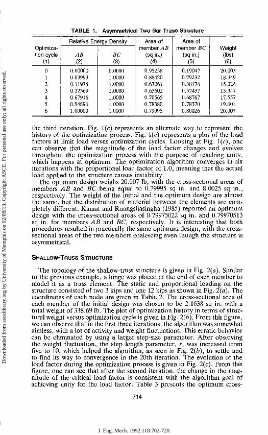
TABLE 1. Asymmetrical Two-Bar Truss Structure

Optimiza­tion cycle

(D 0 1 2 3 4 5 6

Relative Energy Density

AB (2)

0.00000 0.03993 0.11974 0.32369 0.67916 0.94896 1.00000

BC (3)

0.0000 1.0000 1.0000 1.0000 1.0000 1.0000 1.0000

Area of member AB

(sq in.) (4)

0.95238 0.88420 0.67061 0.63602 0.70565 0.78380 0.79995

Area of member BC

(sq in.) (5)

0.19047 0.29232 0.38174 0.52437 0.68767 0.78370 0.80026

Weight (lbs) (6)

20.003 18.349 15.324 15.347 17.557 19.601 20.007

the third iteration. Fig. 1(c) represents an alternate way to represent the history of the optimization process. Fig. 1(c) represents a plot of the load factors at limit load versus optimization cycles. Looking at Fig. 1(c), one can observe that the magnitude of the load factor changes and evolves throughout the optimization process with the purpose of reaching unity, which happens at optimum. The optimization algorithm converges in six iterations with the proportional load factor of 1.0, meaning that the actual load applied to the structure causes instability.

The optimum design weighs 20.007 lb, with the cross-sectional areas of members AB and BC being equal to 0.79995 sq in. and 8.0025 sq in., respectively. The weight of the initial and the optimum design are almost the same, but the distribution of material between the elements are com­pletely different. Kamat and Ruangsilasingha (1985) reported an optimum design with the cross-sectional areas of 0.79975022 sq in. and 0.79970513 sq in. for members AB and BC, respectively. It is interesting that both procedures resulted in practically the same optimum design, with the cross-sectional areas of the two members coalescing even though the structure is asymmetrical.

SHALLOW-TRUSS STRUCTURE

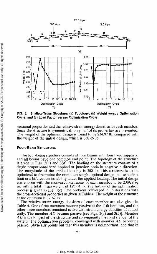
The topology of the shallow-truss structure is given in Fig. 2(a). Similar to the previous example, a hinge was placed at the end of each member to model it as a truss element. The static and proportional loading on the structure consisted of two 3 kips and one 12 kips as shown in Fig. 2(a). The coordinates of each node are given in Table 2. The cross-sectional area of each member of the initial design was chosen to be 2.1638 sq in. with a total weight of 338.69 lb. The plot of optimization history in terms of struc­tural weight versus optimization cycle is given in Fig. 2(b). From this figure, we can observe that in the first three iterations, the algorithm was somewhat aimless, with a lot of activity and weight fluctuations. This erratic behavior can be eliminated by using a larger step-size parameter. After observing the weight fluctuation, the step length parameter, r, was increased from five to 10, which helped the algorithm, as seen in Fig. 2(b), to settle and to find its way to convergence in the 20th iteration. The evolution of the load factor during the optimization process is given in Fig. 2(c). From this figure, one can see that after the second iteration, the change in the mag­nitude of the critical load factor is consistent with the algorithm goal of achieving unity for the load factor. Table 3 presents the optimum cross-

714

J. Eng. Mech. 1992.118:702-720.

Dow

nloa

ded

from

asc

elib

rary

.org

by

Uni

vers

ity o

f M

emph

is o

n 02

/08/

13. C

opyr

ight

ASC

E. F

or p

erso

nal u

se o

nly;

all

righ

ts r

eser

ved.

12.0 kips 3.0 kips 3.0 kips

260^

| 235^

225

220-

1 \ 1

'

/ / /

f 1-4

\ \ \

[

I

\ i

l

\ \ *•«-V

1.05-1

1 00

I . 0.0,

s °-90

^ 0 0 5 „ 0.85

| 0.80

0.75-

\

\

i \

1 1

^ c * i y* *®- ** V** &> >*<

0 2 4 6 8 10 12 14 16 18 20

Optimization Cycle

(b)

0 2 4 6 8 10 12 14 16 18 20

Optimization Cycle (c)

FIG. 2. Shallow-Truss Structure: (a) Topology; (b) Weight versus Optimization Cycle; and (c) Load Factor versus Optimization Cycle

sectional properties and the relative strain energy densities for each member. Since the structure is symmetrical, only half of its properties are presented. The weight of the optimum design is found to be 234.97 lb, compared with the weight of the initial design, which is 338.69 lb.

FOUR-BEAM STRUCTURE

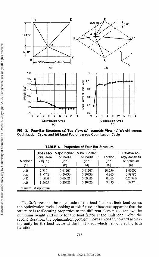
The four-beam structure consists of four beams with four fixed supports, and all beams have one common end point. The topology of the structure is given in Figs. 3(a) and 3(b). The loading on the structure consists of a single proportional load applied at junction node in negative z-direction. The magnitude of the applied loading is 200 lb. This structure is to be optimized to determine the minimum weight optimal design that exhibits a limit or a bifurcation instability under the applied loading. The initial design was chosen with the cross-sectional areas of each member to be 2.0929 sq in. with a total initial weight of 120.64 lb. The history of the optimization process is given in Fig. 3(c). The problem converged in 15 iterations with the cross-sectional properties as given in Table 4. The weight of the structure at the optimum is 77.67 lb.

The relative strain energy densities of each member are also given in Table 4. One of the members became passive at the 11th iteration, and the other three members remained active with strain energy densities of almost unity. The member AD became passive [see Figs. 3(a) and 3(b)]. Member AD is the longest of the structure and consequently the most slender of the system. The optimization problem, converged with member AD becoming passive, physically points out that this member is unimportant, and that in

715

J. Eng. Mech. 1992.118:702-720.

Dow

nloa

ded

from

asc

elib

rary

.org

by

Uni

vers

ity o

f M

emph

is o

n 02

/08/

13. C

opyr

ight

ASC

E. F

or p

erso

nal u

se o

nly;

all

righ

ts r

eser

ved.

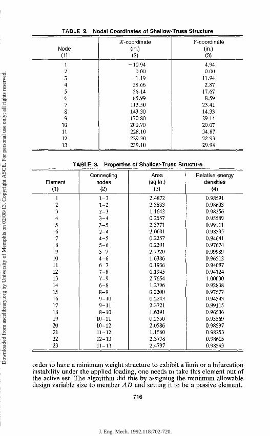
TABLE 2. Nodal Coordinates of Shallow-Truss Structure

Node

(1)

1 2 3 4 5 6 7 8 9

10 11 12 13

Z-coordinate (in.) (2)

-10.94 0.00

-1 .19 28.66 56.14 85.99

113.50 143.30 170.80 200.70 228.10 229.30 239.10

Y-coordinate (in.) (3)

4.94 0.00

11.94 2.87

17.67 8.59

23.41 14.33 29.14 20.07 34.87 22.93 29.94

TABLE 3. Properties of Shallow-Truss Structure

Element

(1)

1 2 3 4 5 6 7 8 9

10 11 12 13 14 15 16 17 18 19 20 21 22 23

Connecting nodes

(2)

1-3 1-2 2 -3 3-4 3-5 2-4 4-5 5-6 5-7 4 -6 6-7 7-8 7-9 6-8 8-9 9-10 9-11 8-10

10-11 10-12 11-12 12-13 11-13

Area (sq in.)

(3)

2.4872 2.3833 1.1642 0.2557 2.3771 2.0601 0.2257 0.2201 2.7720 1.6386 0.1936 0.1945 2.7654 1.2796 0.2200 0.2243 2.3721 1.6391 0.2550 2.0586 1.1560 2.3778 2.4797

Relative energy densities

(4)

0.98591 0.98603 0.98256 0.95589 0.99111 0.98595 0.94641 0.97674 0.99989 0.96512 0.94087 0.94124 1.00000 0.92838 0.97677 0.94543 0.99115 0.96506 0.95569 0.98597 0.98253 0.98605 0.98593

order to have a minimum weight structure to exhibit a limit or a bifurcation instability under the applied loading, one needs to take this element out of the active set. The algorithm did this by assigning the minimum allowable design variable size to member AD and setting it to be a passive element.

716

J. Eng. Mech. 1992.118:702-720.

Dow

nloa

ded

from

asc

elib

rary

.org

by

Uni

vers

ity o

f M

emph

is o

n 02

/08/

13. C

opyr

ight

ASC

E. F

or p

erso

nal u

se o

nly;

all

righ

ts r

eser

ved.

144.0'

60.0'

140

130-

120

§110-

I 100

90

80

70

V

| o . ,

i -i"

0.6-

1 / i

10 12 14 16 10 12 14 16

Optimization Cycle (c)

Optimization Cycle (d)

FIG. 3. Four-Bar Structure: (a) Top View; (b) Isometric View; (c) Weight versus Optimization Cycle; and (d) Load Factor versus Optimization Cycle

Member

(D AB AC AD AE

TABLE 4. Properties of Four-Bar Structure

Cross sec­tional area

(sq in.) (2)

2.7101 1.8762 0.1000 1.5655

Major moment of inertia

(in/) (3)

0.61207 0.29336 0.00083 0.20423

Minor moment of inertia

(in.4) (4)

0.61207 0.29336 0.00083 0.20423

Torsion (in.4) (5)

10.356 4.963 0.013 3.455

Relative en­ergy densities

of optimum (6)

1.00000 0.99786 0.20986" 0.99770

"Passive at optimum.

Fig. 3(d) presents the magnitude of the load factor at limit load versus the optimization cycle. Looking at this figure, it becomes apparent that the structure is reallocating properties to the different elements to achieve the minimum weight and unity for the load factor at the limit load. After the second iteration, the optimization problem moves smoothly toward achiev­ing unity for the load factor at the limit load, which happens at the fifth iteration.

717

J. Eng. Mech. 1992.118:702-720.

Dow

nloa

ded

from

asc

elib

rary

.org

by

Uni

vers

ity o

f M

emph

is o

n 02

/08/

13. C

opyr

ight

ASC

E. F

or p

erso

nal u

se o

nly;

all

righ

ts r

eser

ved.

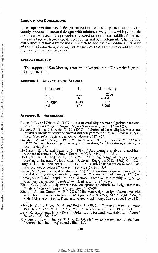
SUMMARY AND CONCLUSIONS

An optimization-based design procedure has been presented that effi­ciently produces structural designs with minimum weight and with geometric nonlinear behavior. The procedure is based on nonlinear stability for struc­tures idealized with two- and three-dimensional beam elements. The method establishes a rational framework in which to address the nonlinear stability of the minimum weight design of structures that exhibit instability under the applied loading conditions.

ACKNOWLEDGMENT

The support of Sun Microsystems and Memphis State University is grate­fully appreciated.

APPENDIX I. CONVERSION TO SI UNITS

To convert To Multiply by

in. mm 25.4 kips N 4,450 in.-kips N-m 113 psi kPa 6,900

APPENDIX II. REFERENCES

Batoz, J. L., and Dhatt, G. (1979). "Incremental displacement algorithms for non­linear problems." Int. J. Numer. Methods in Engrg., 14(8), 1262-1267.

Bergan, P. G., and Soreide, T. H. (1978). "Solution of large displacements and instability problems using the current stiffness parameter." Finite Elements in Non­linear Mechanics, Tapir Press, Geilo, Norway, 647-669.

Gellaty, R.A., and Berke, L. (1971). "Optimal structural design." Report No. AFFDL-TR-70-165, Air Force Flight Dynamics Laboratory, Wright-Patterson Air Force Base, Ohio, Apr.

Hjelmstad, K. D., and Pezeshk, S. (1988). "Approximate analysis of post-limit response of frames." /. Struct. Engrg., ASCE, 114(2), 314-331.

Hjelmstad, K. D., and Pezeshk, S. (1991). "Optimal design of frames to resist buckling under multiple load cases." J. Struct. Engrg., ASCE, 117(3), 914-935.

Hughes, T. J. R., and Pister, K. S. (1978). "Consistent linearization in mechanics of solids and structures." Comput. Struct., 8(2), 391-397.

Kamat,M. P., and Ruangsilasingha, P. (1985). "Optimization of space trusses against instability using design sensitivity derivatives." Engrg. Optimization, 8, 177-188.

Kamat, M. P. (1987). "Optimization of shallow arches against instability using design sensitivity derivatives." Finite Elem. Anal. Des., 3, 277-284.

Khot, N. S. (1981). "Algorithm based on optimality criteria to design minimum weight structures." Engrg. Optimization, 5, 73-90.

Khot, N. S., and Kamat, M. P. (1983). "Minimum weight design of structures with geometric nonlinear behavior." AIAA paper No. 83-0973, AIAA/ASME/ASCE/ AHS 25th Struct., Struct. Dyn., and Mater. Conf., May, Lake Tahoe, Nev., 383-391.

Khot, N. S., Venkayya, V. B. and Berke, L. (1976). "Optimum structural design with stability constraints." Int. J. Num. Methods Engrg., 10(5), 1097-1114.

Levy, R., and Perng, H. S. (1988). "Optimization for nonlinear stability." Comput. Struct, 30(3), 529-535.

Marsden, J. E., and Hughes, T. J. R. (1983). Mathematical foundation of elasticity. Prentice-Hall, Inc., Englewood Cliffs, N.J.

718

J. Eng. Mech. 1992.118:702-720.

Dow

nloa

ded

from

asc

elib

rary

.org

by

Uni

vers

ity o

f M

emph

is o

n 02

/08/

13. C

opyr

ight

ASC

E. F

or p

erso

nal u

se o

nly;

all

righ

ts r

eser

ved.

Olhoff, N., and Taylor, J. E. (1983). "On structural optimization." J. Appl. Mech., 50(46), 1139-1151

Park, J. S., and Choi, K. K. (1990). "Design sensitivity analysis of critical load factor for nonlinear structural systems." Comput. Struct., 36(5), 833-838.

Ramm, E. (1980). "Strategies for tracing the nonlinear response near limit points." Europe-U.S.-Workshop on Nonlinear Finite Elem. Anal, in Struct. Mech., July, Bochum, Germany.

Szyszkowski, W. (1990). "Shape optimization for maximum stability and dynamic stiffness." Proc. of the 3rd Air Force/NASA Symp. on Recent Advances in Mul-tidisciplinary Anal, and Optimization, Anamet Lab, Inc., San Francisco, Calif., 297-302.

Wu, C. C, and Arora, J. S. (1988). "Design sensitivity analysis of nonlinear buckling constraint." Computational Mech., 3, 129-140.

Zienkiewicz, O. C. (1982). The finite element method. 3 Ed., McGraw-Hill, Inc., London, U.K.

APPENDIX III. NOTATION

The following symbols are used in this paper:

(A2)i, (A3)i = major and minor shear area of the cross section for group i;

a, = area of the cross section for group i; a = cross-sectional area;

B(-q) = strain displacement operator; D = elastic moduli; dv = number of design variables; e! = unit vector pointing in positive x-direction; F = vector of gradient of the objective function;

G, = shear modulus of group i; h, h - principal moments of inertia about y- and

z-axes; 1,1 = vector of major and minor moment of iner­

tias; /,, /, = major and minor moment of inertia of the

cross section for group i; J = vector of torsion constants; / = torsion constant; /, = torsion constant of the cross section for group

i; L, = length of member;

M2, M3 = flexural moment acting about y- and z-di­rections;

m2, m3 = applied moments in direction of y and z; N = axial force; P = vector of gradient of the constraint func­

tional; p = applied axial force;

qm = specific weight of the mth group of design variables;

q = vector of the applied forces; ?2> <?3 = applied shear forces in direction of y and z; Q(x) = resultant internal forces;

719

J. Eng. Mech. 1992.118:702-720.

Dow

nloa

ded

from

asc

elib

rary

.org

by

Uni

vers

ity o

f M

emph

is o

n 02

/08/

13. C

opyr

ight

ASC

E. F

or p

erso

nal u

se o

nly;

all

righ

ts r

eser

ved.

r0 = (0, y, z) = vector that points from origin to the point 0.*);

R = stress resultants; T = torque; t = applied torque;

u = displacements; u0 = [u, v, w]' = displacement at the origin of axes (x, y, z);

V2, V3 = shear forces acting in y- and z-directions;

Wi = strain energy potential of the ith group; x = {*!, x2, . . . , xdv} = vector of design variables;

Xj, Xj = minimum and maximum permissible size on design variables;

e0 = [EJ, E2,e3]' = axial and shear stress resultant vector; ti = admissible variations of the displacement

field; Ko = [K1; K2, K4]' = twist- and flexure-stress resultant vector;

A. = [\1; \2, X3, \4 , X5, \6]' = vector of strain measures; S(u) = strain gradient;

II = total potential energy; IT = total potential energy associated with the

optimum design at the nonlinear critical load; «!>o - [4>i, <l>2. <W = vector of rotation of cross section about (x,

y, z) axes; and p, = density of member i.

720

J. Eng. Mech. 1992.118:702-720.

Dow

nloa

ded

from

asc

elib

rary

.org

by

Uni

vers

ity o

f M

emph

is o

n 02

/08/

13. C

opyr

ight

ASC

E. F

or p

erso

nal u

se o

nly;

all

righ

ts r

eser

ved.