On an Estimation Method for an Alternative Fractionally...

Department of Economics and Business

Aarhus University

Fuglesangs Allé 4

DK-8210 Aarhus V

Denmark

Email: [email protected]

Tel: +45 8716 5515

On an Estimation Method for an Alternative Fractionally

Cointegrated Model

Federico Carlini and Katarzyna Łasak

CREATES Research Paper 2014-15

mailto:[email protected]

On an Estimation Method for an Alternative Fractionally

Cointegrated Model

Federico Carlini†

CREATES, Aarhus University, DK

E-mail: [email protected]

Katarzyna Łasak∗†

VU Amsterdam & Tinbergen Institute, NL

E-mail: [email protected]

April 29, 2014

Abstract

In this paper we consider the Fractional Vector Error Correction model proposed in Avarucci

(2007), which is characterized by a richer lag structure than models proposed in Granger (1986)

and Johansen (2008, 2009). We discuss the identification issues of the model of Avarucci (2007),

following the ideas in Carlini and Santucci de Magistris (2014) for the model of Johansen (2008,

2009). We propose a 4-step estimation procedure that is based on the switching algorithm

employed in Carlini and Mosconi (2014) and the GLS procedure in Mosconi and Paruolo

(2014). The proposed procedure provides estimates of the long run parameters of the fractional

cointegrated system that are consistent and unbiased, which we demonstrate by a Monte Carlo

experiment.

Keywords: Error correction model, Gaussian VAR model, Fractional Cointegration, Es-

timation algorithm, Maximum likelihood estimation, Switching Algorithm, Reduced Rank Re-

gression. JEL: C13, C32.

∗Corresponding author’s address: VU Amsterdam – FEWEB, De Boelelaan 1105, 1081 HV Amsterdam, TheNetherlands. Telephone: +31205982260.

†We would like to thank Charles Bos, Søren Johansen, Niels Haldrup, Rocco Mosconi and Morten Nielsen. Thefinancial support from CREATES - Center for Research in Econometric Analysis of Time Series funded by the DanishNational Research Foundation (DNRF78), VU Amsterdam and the Tinbergen Institute is gratefully acknowledged.

1

1 Introduction

The econometrics literature on fractional co-integration has developed rapidly in recent years. An

empirically attractive methodological strategy is to use parametric inference, based on an econo-

metric model that fully describes the system under consideration. It allows identification of the

long-run and short-run structure in the model, as well as of the common stochastic trends and the

impulse response functions. Three different Fractional Vector Error Correction Models (FVECM)

have been proposed in the literature in Granger (1986), Johansen (2008, 2009) and Avarucci (2007).

They turn out to be identical in the simplest case without short run dynamics, but in general case

they are characterized by different lag structures.

The model proposed in Johansen (2008, 2009) has a convenient algebraic structure. The in-

ference for this model has been developed in Johansen and Nielsen (2012). However there exist

identification problems in this model, that have been mentioned in Johansen and Nielsen (2012)

and further discussed in Carlini and Santucci de Magistris (2014).

In this paper we demonstrate that the identification problems also occur but are less severe in

the model proposed by Avarucci (2007) and that statistical inference for this model is different.

The estimation is slightly more complicated due to the multiplicative structure of the parameters

involved, while testing would be less complicated due to the fact that the nesting structure follows

the usual structure of the Vector AutoRegressive (VAR) models. We propose a 4 step algorithm

to estimate the parameters of this model. The algorithm is based on the approach of Carlini

and Mosconi (2014) that maximizes likelihood function using a switching algorithm and a GLS

procedure proposed in Mosconi and Paruolo (2014).

In the Monte Carlo experiment we investigate the small sample properties of the estimates of

all the parameters of this model and we check also the asymptotic properties.

The remainder of the paper is organized as follows. Section 2 presents the FVECM proposed

in Avarucci (2007) and its properties. In Section 3 the identification issues are discussed. Section

4 introduce a 4 step algorithm to estimate the parameters of this model. Section 5 describes the

small sample properties and the asymptotic properties of the parameter estimators by means of a

Monte Carlo experiment. Section 6 concludes. The Appendix gives details on the GLS procedure

in Mosconi and Paruolo (2014). Tables and Figures follow.

2

2 Avarucci model of Fractional Cointegration

The model of Avarucci (2007) is given by the following dynamics

∆dXt = αβ′(∆d−b−∆d)Xt +

k∑j=1

BjLj(∆d−b−∆d)Xt +

k∑j=1

AjLj∆dXt + εt εt ∼ iidN(0,Ω) (1)

where Bj = −(αβ′)Aj . The vector of variables Xt is p−dimensional, the loadings α and the

cointegrating relations β are p × r matrices where 0 ≤ r ≤ p, Aj and Bj , j = 1, . . . , k are p × p

matrices of the short run dynamics. The lag operator L is such that LXt = Xt−1 and the fractional

difference is given by the binomial expansion ∆d := (1− L)d =∑∞

j=0(−1)j(jd

)Lj .

The model can be written in another form. The form proposed is coherent with the represen-

tation in Johansen (2008) . The model in (1) can be reformulated as:

∆dYt = αβ′∆d−bLbYt + εt,

where Lb := 1−∆b is the fractional lag operator and with the restriction Yt =(Ip −

∑kj=1AjL

j)Xt,

or more explicitly by

∆d−b (∆bIp − αβ′Lb

)Ip − k∑j=1

AjLj

Xt = εt. (2)

This model is characterized by a different (and more complicated) lag structure than the model

proposed in Granger (1986)

∆dXt = αβ′(∆d−b −∆d

)Xt−1 +

k∑j=1

ΓjLj∆dXt + εt, (3)

and Johansen (2008, 2009),

∆dXt = αβ′(∆d−b −∆d)Xt +

k∑j=1

ΓjLj(∆d−b −∆d)Xt + εt. (4)

In fact model (1) contains both the usual lags based on a standard lag operator present in

Granger’s model (3) and fractional lags present in the model of (4) Johansen. In the particular case

of d = b = 1 all 3 models reduce to the standard ECM. When the short run dynamics components

3

are made equal to zero (i.e. k = 0) the models are not present, apart for the initial values. The

solution of the Johansen’s model depends on the initial values, for t < 0, while the model of Avarucci

implicitly assumes that the process starts in t = 0.

The moving average representation (MA) of the model (1) is given in Avarucci (2007). Following

his Theorem 2.2, Xt has the representation

Xt = C∆−d+ εt + C∗∆−d+b+ εt + ∆−d+2b

+

t−1∑j=1

Φjεt−j , (5)

where∑∞

j=0 ||Φj ||2 < ∞, and C = β⊥(α′⊥β⊥)−1α′⊥, and C∗ = −[βα′ + Cβα′ + βα′C + Cβα′C],

where Φj , j = 1, . . . , t − 1 are p × p matrices and if c is a generic p × r matrix then c := c(c′c)−1

and c⊥ is a p× (p− r) matrix such that c′⊥c = c′c⊥ = 0. Thus, Xt and β′Xt are Type II I(d) and

I(d− b) processes.

The proof of Theorem 2.2 is largely based on Theorem 8 in Johansen (2008) and the MA

representation (5) is based on the solution given in Johansen (2008, 2009):

Xt = C∆−d+ εt + ∆−(d−b)+ Y +

t + µt, (6)

where µt is a deterministic component generated by initial values, C = β⊥(α′⊥Γβ⊥)−1α′⊥ and

Y +t =

t−1∑n=0

τnεt−n, so Yt is fractional of order zero, thus Xt ∼ I(d), while ∆bXt, β′Xt ∼ I(d− b).

Therefore both models generate the same class of processes. However, in the model proposed by

Avarucci (2007) cointegration always occurs if b > 0 unlike in the model of Johansen (2008, 2009)

where the system can be not cointegrated for b > 0 if αβ′ is a full rank matrix.

The nesting structure of the Avarucci model also differs from the nesting structure of the Jo-

hansen (2008, 2009) model and it follows the VAR structure. If we define the model

Hr,k : ∆d−b(∆bIp − αβ′Lb)(Ip −k∑

i=1

AiLi)Xt = εt, r = 0, . . . , p

4

then, the nesting structure of the Avarucci’s model is given by

H0,0 ⊂ H0,1 ⊂ H0,2

∩ ∩ ∩

H1,0 ⊂ H1,1 ⊂ H1,2

∩ ∩ ∩

H2,0 ⊂ H2,1 ⊂ H2,2

For example the inclusion H2,1 ⊂ H2,2 can be tested by A2 = 0 and the inclusion H1,1 ⊂ H2,1 can

be tested on a rank restriction on the matrix αβ′. Moreover, it is simple to prove that the model

H0,1 is not nested in H2,0 because the term αβ′Lb is zero in H0,1.

The nesting structure of the Johansen model is more complicated, see Carlini and Santucci de

Magistris (2014) for the details. Therefore, the inference for these two models should be different,

despite of the fact that they both generate the same class of processes.

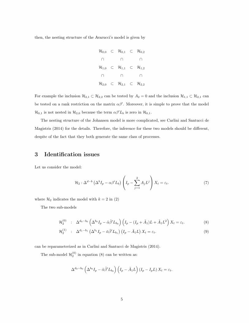
3 Identification issues

Let us consider the model:

H2 : ∆d−b (∆bIp − αβ′Lb

)Ip − 2∑j=1

AjLj

Xt = εt. (7)

where H2 indicates the model with k = 2 in (2)

The two sub-models

H(0)2 : ∆d0−b0

(∆b0Ip − αβ′Lb0

)(Ip − (Ip + A1)L+ A1L

2)Xt = εt. (8)

H(1)2 : ∆d1−b1


) (Ip − A1L

)Xt = εt. (9)

can be reparameterized as in Carlini and Santucci de Magistris (2014).

The sub-model H(0)2 in equation (8) can be written as:

∆d0−b0(

∆b0Ip − αβ′Lb0

)(Ip − A1L

)(Ip − IpL)Xt = εt.

5

or equivalently as

∆d0−b0(

∆b0Ip − αβ′Lb0

)(Ip − A1L

)∆IpXt = εt

Therefore,

H(0)2 : ∆d0−b0+1


)(Ip − A1L

)Xt = εt (10)

Now, let us compare the sub-models (9) and (10). It is clear that the equations (10) and (9)

reparameterize when αβ′ = αβ′, A1 = A1, b1 = b0 and d0 − b0 + 1 = d1 − b1. Hence, H2,0 = H2,1

iff d0 + 1 = d1.

Furthermore, note that the sub-model H(0)2 is a sub-model of the model H2, where we impose

the restriction A2 + A1 − Ip = 0. Instead, the sub-model H(1)2 is the sub-model of the model H2

where we impose the restriction A2 = 0.

Therefore, the parameter b is always identified. It seems that an identification problem could

occur as in Johansen (2008) and Johansen and Nielsen (2010) for certain values of d. If we want to

avoid identification issues, we only need to assume that the characteristic polynomial

Π(z) =

Ip − k∑j=1

Ajzj

has roots outside of the unit circle, which is already assumed in Avarucci (2007). Therefore the

identification problem for the parameter d is not present.

However, the problem of identification can arise when αβ′ = 0. In this situation, the eq. (2) is

given by

∆d

Ip − k∑j=1

AjLj

Xt = εt

and the parameter b is not identified. This special feature of the model has been used in Łasak

(2010) to propose a sup-test for no cointegration.

Furthermore, suppose that b = 1 and αβ′ is a full rank matrix, then we have

∆d−1(∆Ip − αβ′L)(Ip −A1L)Xt = εt

This is equal to

∆d−1(Ip − (αβ′ + Ip)L)(Ip −A1L)Xt = εt

6

If αβ′ + Ip = A1, then an identification problem arises because the two factors of the last equation

commute. Therefore the cases of no-cointegration and the cointegration of a full rank should be

treated separately.

4 Estimation Algorithm

In this section we propose an estimation procedure for the model of Avarucci (2007). To keep the

presentation simple, we consider the case d = b. Using the approach of Carlini and Mosconi (2014),

the likelihood function can be maximized with a switching algorithm. The model is given by:

(∆dIp − α1β′1Ld) ·A(L) ·Xt = εt εt ∼ N(0,Ω)

where A(L) = Ip −A1L− · · · −AkLk and α1 and β1 are a p× r matrices.

The model can be written as:

∆dXt = A∆dZt + α1β′1LdXt − α1β

′1ALdZt + εt t = 1, . . . , T

where

Zt =

LXt

L2Xt

...

LkXt

and

A = [A1 : A2 : · · · : Ak]

where A is the horizontal concatenation of the matrices A1, . . . , Ak.

The likelihood is maximized using the following switching procedure:

• A- step: given α1, β1 and Ω we estimate A. Defining:

YAt = ∆dXt − α1β′1LdXt

WAt =

∆dZt

LdZt

7

and hence

YAt = [I : −α1β1](I2 ⊗A)WAt + εt

This can be solved by GLS on A (see Mosconi and Paruolo (2014) and Appendix). So, in this

case, H = [I : −α1β1] and θ′ = (I2 ⊗A).

• β1-step: given A and Ω and α1, we estimate β1. Defining

Ybt = ∆dXt −A∆dZt

and

Wbt = LdXt −ALdZt,

we solve the following problem:

Ybt = α1β′1Wbt + εt

This can be solved by GLS as in Mosconi and Paruolo (2014), where H = α1 and θ′ = β′1.

• α1−step: given A,Ω and β1, we estimate α1. Defining

Yat := Ybt

and

Wat = β′1Wbt

we solve the following problem:

Yat = α1Wat + εt.

Again, this can be solved by GLS as in Mosconi and Paruolo (2014), where H = I2 and

θ′ = α1.

• Ω−step: given a1, β1, A we estimate Ω. The likelihood is maximized with respect to Ω by

Ω =1

T

T∑t=1

εtε′t

defining εt = ∆dXt −A∆dZt − a1β1LdXt + a1β1ALdZt.

8

Iterating these steps and changing the parameter d in a maximization algorithm, the likelihood is

maximized and we get d, a1, b1, A, Ω.

5 Simulation experiment.

The Monte Carlo works as follows. We generate N = 1, 000 Monte Carlo replication from the

following DGP

(∆d0Ip − α0β′0Ld0

)(Ip −A1,0L−A2,0L2)Xt = εt εt ∼ i.i.d.N(0,Ω0), t = 1, . . . , T

where

A0 = [A1,0 : A2,0] =

0.2 −0.6

−0.3 0.5

−0.2 0.1

0.2 −0.5

,

α0 =

−0.5

0.5

, β0 =

1

−0.2

and Ω0 =

1 0

0 1

.and T = 100, 250, 10000. The values chosen for d0 are 0.3, 0.6 and 0.9. The data are generated with

a modified version of the program provided in Jensen (2014).

For each run of the Monte Carlo, we fit the model

(∆dIp − αβ′Ld)(Ip −A1L−A2L2)Xt = εt, εt ∼ iidN(0,Ω) (11)

using the switching algorithm described in Section 4. When we maximize the likelihood, the initial

value for the parameter d is chosen in a neighbourhood of the true value d0, while the initial values

for α, β and Ω are imposed to be α0, β0 and Ω0. The maximization routine climbs the likelihood

over values of d in [0.1, 2] in order to avoid negative - or close to zero - d estimates. Hence, we

collect the estimates d, α, β, A1, A2 and Ω for each iteration of the Monte Carlo.

To simplify the exposition, we introduce new notation for the elements of the matrices in the

model (11). We call the elements of the matrices

α =

α1

α2

, β =

1

β1

, A =

a(1)11 a

(1)12 a

(2)11 a

(2)12

a(1)21 a

(1)22 a

(2)21 a

(2)22

and Ω =

ω11 ω12

ω21 ω21

9

where ω21 = ω12.

When the data are generated with fractional parameters d0 = 0.3 and d0 = 0.6, the bias and

the standard deviations of the Monte Carlo estimates are given in the Tables 1-12 in Appendix.

From these Tables emerges that if T increases the bias and the standard error of α, β,Ω decrease,

while if T increases just the standard error of A1 and A2 decrease.

The plots in the appendix are the Monte Carlo distributions of some of the parameters estimates

in model (11), smoothed by a Gaussian Kernel when d0 = 0.6 and T = 100 and T = 10, 000.

The top-left plot in Figure 1 shows that the distribution of d when T = 250 has the estimated

values centred in two zones. This is due to the fact that the maximization algorithm converged at

values of d on the boundary of the interval d = [0.1, 2], giving as a result a bimodal distribution

where the first mode is in 0.1 and the second one centred close to d = 0.6. This happens when

the sample is small because the estimates of d, sometimes, tend to assume values close to zero or

negative. This also explains why the distributions of the parameters α, β,A1 and A2 are skewed.

Instead the plot in Figure 2 shows that the distribution of d when T = 10, 000 is uni-modal and

symmetric as the distributions of all the other parameters.

Another characteristic of the algorithm is that if we generate data with d0 = 0.9 and a large

T , the maximization routine rarely is not able to converge, stopping at d = 0.1 with an allert

of non-convergence. We noted that the number of iterations for the convergence of the switching

algorithm when d is close to 0.9 becomes so big that we could need more than 10,000 iterations even

if the starting values of α, β and Ω are imposed on their true values. This phenomenon becomes

cumbersome in terms of speed and in terms of reliability of the estimates of the parameters. Hence,

further research has to be done to improve the convergence properties of this algorithm when the

data generating process is generated by a fractional parameter d0 close to 1.

6 Conclusions

In this paper we consider estimation of an alternative fractionally cointegrated model that has been

proposed in Avarucci (2007) and Avarucci and Velasco (2010). This model is characterized by a

richer lag structure than models previously proposed by Granger (1986) and Johansen (2008, 2009).

We present a 4 step algorithm to estimate this model. The algorithm is based on the approach of

Carlini and Mosconi (2014) that maximizes likelihood function using a switching algorithm and the

10

GLS procedure as in Mosconi and Paruolo (2014). We study small sample properties of the estimates

of all the parameters of fractionally cointegrated model obtained using the proposed algorithm. We

also demonstrate by a Monte Carlo experiment that the proposed procedure provides estimates of

the long run parameters of the fractionally cointegrated system that are consistent and unbiased.

Appendix

The following algorithm describes how to estimate a bilinear form with a GLS model. Further

details can be found in Mosconi and Paruolo (2014).

Consider the following equation

Yt = Hθ′Wt + εt t = 1, . . . , T

εt ∼ iidN(0,Ω), vec(θ) = Kψ

where Yt and Xt are respectively py × 1 and px × 1 vectors, H and θ are respectively py × r and

px × r matrices. Then, we can estimate ψ as

ψ = (K ′(H ′Ω−1H ⊗ Sxx)K)−1K ′vec(SxyΩ−1H)

where Sww =∑T

t=1WtW′t and Swy =

∑Tt=1WtY

′t .

11

Tables

d α1 α2 β1 ω11 ω12 ω22

Bias 0.029 -0.584 2.110 -4.143 -0.065 0.004 -0.070St. Error 0.292 3.834 6.245 88.426 0.142 0.098 0.135

Table 1: Bias and Standard Error when the DGP is generated with d0 = 0.3 and T = 100

a(1)11 a

(1)12 a

(1)21 a

(1)22 a

(2)11 a

(2)12 a

(2)21 a

(2)22

Bias 0.480 1.200 0.415 -0.445 0.169 -0.158 -0.089 0.661St. Error 0.618 0.760 0.938 0.691 0.557 0.370 0.644 0.589


d α1 α2 β1 ω11 ω12 ω22

Bias 0.023 -0.398 0.635 -2.252 -0.027 0.002 -0.024St. Error 0.217 1.447 2.013 108.134 0.089 0.063 0.088


a(1)11 a

(1)12 a

(1)21 a

(1)22 a

(2)11 a

(2)12 a

(2)21 a

(2)22

Bias 0.459 1.238 0.683 -0.467 0.169 -0.138 -0.181 0.538St. Error 0.314 0.326 0.351 0.336 0.259 0.190 0.267 0.232


d α1 α2 β1 ω11 ω12 ω22

Bias -0.001 -0.002 0.007 -0.002 -0.001 -0.001 -0.001St. Error 0.026 0.058 0.060 0.105 0.014 0.010 0.014


a(1)11 a

(1)12 a

(1)21 a

(1)22 a

(2)11 a

(2)12 a

(2)21 a

(2)22

Bias 0.401 1.299 0.798 -0.500 0.200 -0.101 -0.200 0.501St. Error 0.022 0.020 0.020 0.024 0.018 0.018 0.018 0.016


12

d α1 α2 β1 ω11 ω12 ω22

Bias -0.039 -0.331 2.002 -0.649 -0.063 0.004 -0.073St. Error 0.404 2.732 5.298 21.586 0.142 0.098 0.134


a(1)11 a

(1)12 a

(1)21 a

(1)22 a

(2)11 a

(2)12 a

(2)21 a

(2)22

Bias 0.521 1.279 0.423 -0.445 0.117 -0.168 -0.114 0.630St. Error 0.535 0.545 0.811 0.676 0.466 0.342 0.569 0.545


d α1 α2 β1 ω11 ω12 ω22

Bias -0.027 -0.202 0.684 0.082 -0.026 0.002 -0.025St. Error 0.281 0.997 2.036 7.082 0.089 0.063 0.087

Table 9: Bias and Standard Error when the DGP is generated with d0 = 0.6 and T = 250.

a(1)11 a

(1)12 a

(1)21 a

(1)22 a

(2)11 a

(2)12 a

(2)21 a

(2)22

Bias 0.492 1.291 0.657 -0.455 0.136 -0.150 -0.178 0.538St. Error 0.287 0.274 0.312 0.394 0.250 0.193 0.254 0.215

Table 10: Bias and Standard Error when the DGP is generated with d0 = 0.6 and T = 250.

d α1 α2 β1 ω11 ω12 ω22

Bias 0.000 -0.003 0.003 -0.000 0.000 -0.000 -0.000St. Error 0.024 0.031 0.028 0.047 0.014 0.010 0.014


a(1)11 a

(1)12 a

(1)21 a

(1)22 a

(2)11 a

(2)12 a

(2)21 a

(2)22

Bias 0.401 1.300 0.799 -0.500 0.199 -0.101 -0.199 0.500St. Error 0.023 0.020 0.019 0.027 0.019 0.020 0.019 0.016


13

Figures

−0.5 0 0.5 1 1.5 2 2.50

0.2

0.4

0.6

0.8

1

1.2

1.4d Kernel p.d.f.

−100 −80 −60 −40 −20 0 20 400

0.05

0.1

0.15

0.2

0.25

0.3

0.35

0.4

0.45

0.5

α1 Kernel p.d.f.

−80 −60 −40 −20 0 20 40 600

0.05

0.1

0.15

0.2

0.25

0.3

0.35

0.4

0.45

α2 Kernel p.d.f.

−1500 −1000 −500 0 500 10000

0.5

1

1.5

2

2.5

3

3.5x 10

−3 β1 Kernel p.d.f.

−6 −4 −2 0 2 4 6 8 10 120

0.1

0.2

0.3

0.4

0.5

0.6

0.7

0.8

0.9

1

a11(1) Kernel p.d.f.

−20 −15 −10 −5 0 5 100

0.2

0.4

0.6

0.8

1

1.2

1.4


−20 −15 −10 −5 0 5 100

0.1

0.2

0.3

0.4

0.5

0.6

0.7

0.8

0.9


−10 −8 −6 −4 −2 0 2 4 60

0.1

0.2

0.3

0.4

0.5

0.6

0.7


−8 −6 −4 −2 0 2 4 6 8 100

0.2

0.4

0.6

0.8

1

1.2

1.4


−6 −4 −2 0 2 4 60

0.2

0.4

0.6

0.8

1

1.2

1.4


−6 −4 −2 0 2 4 6 8 10 120

0.2

0.4

0.6

0.8

1

1.2

1.4


−4 −2 0 2 4 6 8 10 120

0.2

0.4

0.6

0.8

1

1.2

1.4


Figure 1: Smoothed Kernel distribution of the estimators of the model (11) when d0 = 0.6 andT = 100

14

0.5 0.55 0.6 0.650

2

4

6

8

10

12

14

16d Kernel p.d.f.

−0.65 −0.6 −0.55 −0.5 −0.45 −0.4 −0.35 −0.30

2

4

6

8

10

12

14

α1 Kernel p.d.f.

0.35 0.4 0.45 0.5 0.55 0.6 0.65 0.70

2

4

6

8

10

12

14

α2 Kernel p.d.f.

−0.45 −0.4 −0.35 −0.3 −0.25 −0.2 −0.15 −0.1 −0.05 00

1

2

3

4

5

6

7

8

9

β1 Kernel p.d.f.

0.5 0.55 0.6 0.65 0.70

2

4

6

8

10

12

14

16


0.55 0.6 0.65 0.7 0.75 0.80

2

4

6

8

10

12

14

16

18

20


0.42 0.44 0.46 0.48 0.5 0.52 0.54 0.56 0.580

5

10

15

20

25


−0.1 −0.05 0 0.05 0.1 0.150

2

4

6

8

10

12

14


−0.08 −0.06 −0.04 −0.02 0 0.02 0.04 0.06 0.080

5

10

15

20

25


−0.1 −0.08 −0.06 −0.04 −0.02 0 0.02 0.04 0.06 0.080

2

4

6

8

10

12

14

16

18

20


−0.1 −0.08 −0.06 −0.04 −0.02 0 0.02 0.04 0.06 0.080

2

4

6

8

10

12

14

16

18

20


−0.06 −0.04 −0.02 0 0.02 0.04 0.06 0.080

5

10

15

20

25


Figure 2: Smoothed Kernel distribution of the estimators of the model (11) when d0 = 0.6 andT = 105

15

References

[1] Avarucci, M. (2007), Three Essays on Fractional Cointegration, PhD Thesis, University of

Rome "Tor Vergata".

[2] Avarucci, M., Velasco C. (2009), A Wald Test for the Cointegration Rank in Nonstationary

Fractional Systems, Journal of Econometrics, 151, 178-189.

[3] Carlini, F., Mosconi, R. (2014), Twice Integrated Models, Manuscript.

[4] Carlini, F., Santucci de Magistris, P. (2014), On the identification of fractionally cointegrated

VAR models with the F(d) condition, CREATES Research Paper 2013-44.

[5] Granger, C. W. J. (1986), Developments in the Study of Cointegrated Economic Variables,

Oxford Bulletin of Economics and Statistics, 48, 213-28.

[6] Jensen, A. N. (2014), Efficient simulation of the Johansen-Nielsen model, University of Copen-

hagen, working paper.

[7] Johansen, S. (2008), A representation theory for a class of vector autoregressive models for

fractional processes, Econometric Theory, 24, 651-676.

[8] Johansen, S. (2009), Representation of cointegrated autoregressive processes with application

to fractional cointegration, Econometric Reviews, 28, 121-145.

[9] Johansen, S., Nielsen, M. Ø. (2012), Likelihood inference for a fractionally cointegrated vector

autoregressive model, Econometrica, 80, 2667-2732.

[10] Łasak, K. (2008), Maximum likelihood estimation of fractionally cointegrated systems, CRE-

ATES Research Paper 2008-53.

[11] Łasak, K. (2010), Likelihood based testing for no fractional cointegration, Journal of Econo-

metrics, 158, 67-77.

[12] Mosconi, R., Paruolo, P. (2014), Rank and order conditions for identification in simultaneous

system of cointegrating equations with integrated variables of order two, MPRA Paper 53589.

16

Research Papers 2013

2013-49: Peter Christoffersen, Vihang R. Errunza, Kris Jacobs and Xisong Jin: Correlation Dynamics and International Diversification Benefits

2013-50: Georgios Effraimidis and Christian M. Dahl: Nonparametric Estimation of Cumulative Incidence Functions for Competing Risks Data with Missing Cause of Failure

2013-51: Mehmet Caner and Anders Bredahl Kock: Oracle Inequalities for Convex Loss Functions with Non-Linear Targets

2013-52: Torben G. Andersen, Oleg Bondarenko, Viktor Todorov and George Tauchen: The Fine Structure of Equity-Index Option Dynamics

2014-01 Manuel Lukas and Eric Hillebrand: Bagging Weak Predictors

2014-02: Barbara Annicchiarico, Anna Rita Bennato and Emilio Zanetti Chini: 150 Years of Italian CO2 Emissions and Economic Growth

2014-03: Paul Catani, Timo Teräsvirta and Meiqun Yin: A Lagrange Multiplier Test for Testing the Adequacy of the Constant Conditional Correlation GARCH Model

2014-04: Timo Teräsvirta and Yukai Yang: Linearity and Misspecification Tests for Vector Smooth Transition Regression Models

2014-05: Kris Boudt, Sébastien Laurent, Asger Lunde and Rogier Quaedvlieg: Positive Semidefinite Integrated Covariance Estimation, Factorizations and Asynchronicity

2014-06: Debopam Bhattacharya, Shin Kanaya and Margaret Stevens: Are University Admissions Academically Fair?

2014-07: Markku Lanne and Jani Luoto: Noncausal Bayesian Vector Autoregression

2014-08: Timo Teräsvirta and Yukai Yang: Specification, Estimation and Evaluation of Vector Smooth Transition Autoregressive Models with Applications

2014-09: A.S. Hurn, Annastiina Silvennoinen and Timo Teräsvirta: A Smooth Transition Logit Model of the Effects of Deregulation in the Electricity Market

2014-10: Marcelo Fernandes and Cristina M. Scherrer: Price discovery in dual-class shares across multiple markets

2014-11: Yukai Yang: Testing Constancy of the Error Covariance Matrix in Vector Models against Parametric Alternatives using a Spectral Decomposition

2014-12: Stefano Grassi, Nima Nonejad and Paolo Santucci de Magistris: Forecasting with the Standardized Self-Perturbed Kalman Filter

2014-13: Hossein Asgharian, Charlotte Christiansen and Ai Jun Hou: Macro-Finance Determinants of the Long-Run Stock-Bond Correlation: The DCC-MIDAS Specification

2014-14: Mikko S. Pakkanen and Anthony Réveillac: Functional limit theorems for generalized variations of the fractional Brownian sheet

2014-15: Federico Carlini and Katarzyna Łasak: On an Estimation Method for an Alternative Fractionally Cointegrated Model

On an Estimation Method for an Alternative Fractionally...

Documents

Transcript of On an Estimation Method for an Alternative Fractionally...