Weighted Maximum Likelihood for Dynamic Factor Analysis...

Weighted Maximum Likelihood for Dynamic Factor Analysis

and Forecasting with Mixed Frequency Data

F. Blasques (a), S.J. Koopman(a,b), M. Mallee(a) and Z. Zhang (a)∗

(a) VU University Amsterdam & Tinbergen Institute Amsterdam

(b) CREATES, Aarhus University, Denmark

September 30, 2015

Abstract

For the purpose of forecasting key macroeconomic or financial variables from a high-

dimensional panel of mixed frequency time series variables, we adopt the dynamic

factor model and propose a weighted likelihood-based method for the estimation of

the typically high-dimensional parameter vector. The loglikelihood function is split

into two parts that are weighted differently. The first part is associated with the key

variables while the second part is associated with the related variables which possibly

contribute to the forecasting of the key variables. We derive asymptotic properties,

including consistency and asymptotic normality, of the weighted maximum likelihood

estimator. We show that this estimator outperforms the standard likelihood-based

estimator in approximating the true unknown distribution of the data as well as in out-

of-sample forecasting accuracy. We also verify the new estimation method in a Monte

Carlo study and investigate the effect of different weights in different scenarios. When

forecasting gross domestic product growth, this key variable is typically observed at

a low (quarterly) frequency while the supporting variables are observed at a high

(monthly) frequency. For such a mixed frequency high-dimensional dataset, we adopt

a low frequency dynamic factor model and discuss the computational efficiencies of

this approach. In an extensive empirical study for the U.S. economy, we present

improvements in forecast precision when the weighted likelihood-based estimation

procedure is adopted.

Keywords: Asymptotic theory, Forecasting, Kalman filter, Nowcasting, State space.

JEL classification: C13, C32, C53, E17.

1 Introduction

The forecasting of macroeconomic and financial time series variables is of key importance

for economic policy makers. Reliable short-term forecasts are especially in high demand

when the economic environment is uncertain as we have witnessed in the years during

∗S.J. Koopman acknowledges support from CREATES, Center for Research in Econometric Analysis ofTime Series (DNRF78), funded by the Danish National Research Foundation. Emails: [email protected],[email protected], [email protected] and [email protected]

1

and after the financial crisis that started in 2007. Many different model-based approaches

exist for this purpose, ranging from basic time series models to sophisticated structural

dynamic macroeconomic models. The underlying idea of the dynamic factor model is to

associate a relatively small set of factors to a high-dimensional panel of economic variables

that includes the variable of interest and related variables. The dynamic factor model has

become a popular tool for the short-term forecasting of the variable of interest, amongst

practitioners and econometricians. This is mainly due to their good forecast performance

as shown in many studies.

The estimation of the parameters in a dynamic factor model is a challenging task

given the high-dimensional parameter vector that mostly consists of factor loading coef-

ficients. A likelihood-based approach in which the likelihood function is evaluated by the

Kalman filter and numerically maximized with respect to the parameter vector is origi-

nally proposed by Engle and Watson (1981) for a model with one dynamic factor. Watson

and Engle (1983) base their estimation procedure on the expectationmaximization (EM)

algorithm; see also Quah and Sargent (1993). Approximate likelihood-based procedures

are developed by Doz, Giannone, and Reichlin (2011) and Banbura and Modugno (2014).

Brauning and Koopman (2014) and Jungbacker and Koopman (2015) propose efficient

transformations of the model to facilitate parameter estimation for high-dimensional dy-

namic factor models. We restrict ourselves in this study to these likelihood-based estima-

tion procedures.

Motivation

An important application of dynamic factor models is their use in the forecasting of

growth in gross domestic product (GDP). A typically high-dimensional panel of macroe-

conomic variables is used to construct factors for the purpose of facilitating the forecasting

of GDP growth. Empirical evidence is given by, amongst others, Stock and Watson (2002)

and Giannone, Reichlin, and Small (2008) for the U.S., Marcellino, Stock, and Watson

(2003) and Runstler et al. (2009) for the euro area, and Schumacher and Breitung (2008)

for Germany. In all these studies, the problem of mixed frequency data arises since the

variable of interest GDP growth is observed at a quarterly frequency while the other

macroeconomic variables are observed at a monthly frequency. The treatment of mixed

frequency data in a dynamic factor model is therefore important for forecasting, nowcast-

ing and backcasting GDP growth. The use of the dynamic factor model in this context

is subject to two fundamental characteristics. First, the use of the factors for extracting

commonalities in the dynamics in the variables is intended to provide a parsimonious way

to link the variables of interest with the related variables. The dynamic factor model

is not designed to provide a correct and exact representation of the true unknown data

generating process for all variables in the panel. Instead, the factors provide a conve-

nient tool to model relations that are potentially very complex. Second, the variable of

interest and the related variables in the dynamic factor model are observed at different

frequencies and play different roles. In particular, we wish to obtain accurate forecasts for

2

the variable of interest that is observed at a low frequency (quarterly) while the related

high frequency (monthly or weekly) variables play a more secondary role as instruments

to improve the forecasting accuracy of the key variable. These two fundamental charac-

teristics of the dynamic factor model for macroeconomics play an important role in our

parameter estimation procedure which is designed to establish a framework in which the

standard maximum likelihood estimator can be improved upon. Next we discuss the two

characteristics of the model in more detail.

Weighted likelihood-based estimation

To address the notion that a single or a small selection of variables in a dynamic

factor model are of key interest while the others can be regarded as instruments, we

present a weighted likelihood-based estimation procedure for the purpose of providing a

more accurate forecasting performance than the standard maximum likelihood estimator.

Our proposed weighted maximum likelihood estimator gives simply more weight to the

likelihood contribution from the variable of interest. For example, for the nowcasting and

forecasting of quarterly growth in gross domestic product, referred to as GDP growth,

more weight can be given to likelihood contribution from GDP growth in comparison to

the other, related variables in the dynamic factor model. The variable-specific weights

introduced by this novel weighted ML estimator differ considerably from other weighted

ML estimators proposed in the literature that introduce observation-specific weights in

the likelihood function. The local ML estimators studied in Tibshirani and Hastie (1987),

Staniswalis (1989) and Eguchi and Copas (1998) assign a weight to each observation that

depends on the distance to a given fixed point. The robust ML estimator of Markatou,

Basu, and Lindsay (1997, 1998) down-weights observations that are inconsistent with

the postulated model. Similarly, Hu and Zidek (1997) devise a general principle of rele-

vance that assigns different weights to different observations in an ML setting. In small

samples, this type of estimator can provide important gains in the trade-off between bias

and precision of the ML estimator. The large sample properties of these estimators are

established in Wang, van Eeden, and Zidek (2004) for given weights, and Wang and Zidek

(2005) provide a method for estimating the weights based on cross-validation. Contrary

to these examples, we propose a weighted ML estimator that gives higher weight to a

subset of a random vector, i.e. to an entire random scalar sequence within the mod-

eled multivariate stochastic process. We discuss the asymptotic properties of this novel

weighted maximum likelihood estimator and we show that the estimator is consistent and

asymptotically normal. We further verify our new approach in a Monte Carlo study to

investigate the effect of different choices for the weights in different scenarios. We also

adopt the weighted likelihood function for parameter estimation in our empirical study

concerning the nowcasting and forecasting of US GDP growth based on a full system

dynamic factor model with mixed frequency variables.

3

Mixed Frequency

The common treatments of mixed frequency data are Bridge models and Mixed Data

Sampling (MIDAS) models. In Bridge models the high frequency data are forecast up to

the desired forecast horizon in a separate time series model. These forecasts are then ag-

gregated to the lower frequency and are used as explanatory variables in a lower frequency

time series model as contemporaneous values. Trehan (1989) is the first application of

Bridge equations in our setting; see also Baffigi, Golinelli, and Parigi (2004) and Go-

linelli and Parigi (2007) for more recent uses of Bridge models. The MIDAS approach of

Ghysels, Santa-Clara, and Valkanov (2006) regresses the low frequency time series vari-

able of interest on the related high frequency variables; the dynamics of the regressors

are not considered by the model. The high frequency regressors are not aggregated but

each individual lag has its own regression coefficient. To avoid parameter proliferation,

these coefficients are subject to specific weighting functions. Foroni, Marcellino, and

Schumacher (2015) propose the use of unconstrained distributed lags and refer to this

approach as unrestricted MIDAS (U-MIDAS).

Dynamic factor models and vector autoregressive (VAR) models can also be adapted

to handle mixed frequency data. The study of Mariano and Murasawa (2003) is the first

to illustrate how a small-scale dynamic factor model can be adapted for mixed frequency

data. The model is formulated in state space form with a monthly time index. The

monthly and quarterly variables are then driven by a single monthly dynamic factor and

by an idiosyncratic factor for each individual series. The Kalman filter treats the missing

observations in the quarterly which occur during the first two months of the quarter. VAR

models for mixed frequency time series has originally proposed by Zadrozny (1990). In

this approach the model also operates at the highest frequency in the data and variables

which are observed at a lower frequency are viewed as being periodically missing. Mittnik

and Zadrozny (2005) report promising results based on this original approach for the

forecasting of German growth in gross domestic product. Ghysels (2012) generalizes the

MIDAS approach for the mixed frequency VAR (MF-VAR). Schorfheide and Song (2013)

develop a MF-VAR model that allows some series to be observed at monthly and others

at quarterly frequencies, using Bayesian state space methods. Their empirical findings for

a large-scale economic VAR are highly promising: within-quarter monthly information

leads to drastic improvements in short-horizon forecasting performance. Bai, Ghysels,

and Wright (2011) examine the relationship between MIDAS regressions and state space

models applied to mixed frequency data. They conclude that the Kalman filter forecasts

are typically slightly better, but MIDAS regressions can be more accurate if the state

space model is misspecified or over-parameterized. Kuzin, Marcellino, and Schumacher

(2011) compare the accuracy of Euro Area GDP growth forecasts from MIDAS regressions

and MF-VARs estimated by maximum likelihood.

Marcellino, Carriero, and Clark (2014) propose a Bayesian regression model with

stochastic volatility for producing current-quarter forecasts of GDP growth with a large

range of available within-the-quarter monthly observations of economic indicators. Each

4

time series of monthly indicators is transformed into three quarterly time series, each

containing observations for the first, second and third month of the quarter. We adopt

their overall approach but apply it to the dynamic factor model and formalize it within

the state space modeling framework in a mixed frequency data setting. Similar ideas

are developed for periodic systems in the control engineering literature; see Bittanti and

Colaneri (2000, 2009). In the econometrics literature and for vector autoregressive sys-

tems, such ideas are explored in Chen, Anderson, Deistler, and Filler (2012), Ghysels

(2012), Foroni, Gurin, and Marcellino (2015) and Ghysels, Hill, and Motegi (2015).

Outline

The outline of the paper is as follows. In Section 2 we present our weighted maximum

likelihood approach that is introduced to increase the influence of the key variables in

the estimation process for a joint multivariate dynamic model. Asymptotic properties of

the resulting estimator are derived and we explore its small-sample properties in a Monte

Carlo study. In Section 3 we show how mixed frequency dynamic factor models can be

specified as observationally equivalent low frequency dynamic factor models. In many

cases the new formulations lead to computational gains. In Section 4 we present and

explore the results of our empirical study concerning US GDP growth. We compare the

nowcasting and forecasting accuracies of our new approach with those of a benchmark

model. We also establish the empirical relevance of the weighted estimation method of

Section 2. Section 5 summarizes and concludes.

2 Weighted Maximum Likelihood Estimation: method and

properties

We represent our high-dimensional unbalanced panel of time series as the column vector

zt for which we have observations from t = 1, . . . , T where T is the overall time series

length. An unbalanced panel refers to the case where we have observations for some of

the variables in the vector zt. We assume that at least some obervations are available for

each variable in zt, for t = 1, . . . , T . The entries for which no observations are available in

zt are treated as missing at random. We decompose zt into variables of interest in yt and

related variables in xt, we have zt = (y′t, x′t)′ where a′t is the transpose of column vector

at. The dimension Ny of yt is small and typically equal to one while the dimension Nx

of xt can be large. Hence the dimension Nz of zt is also large since Nz = Ny + Nx. It

is assumed that all time series variables in zt have zero mean and are strictly stationary.

The basic dynamic factor model for zt can be represented by zt = Λft + εt or(yt

xt

)=

[Λy

Λx

]ft +

(εy,t

εx,t

), ft = Φft−1 + ηt, (1)

5

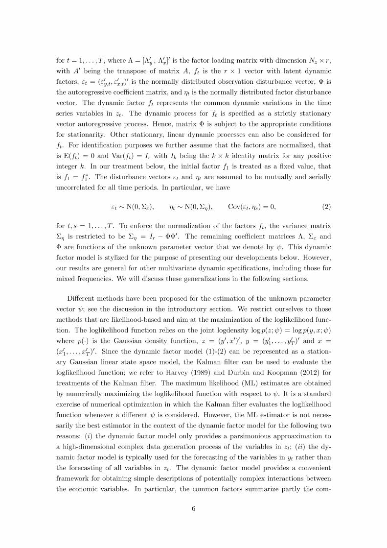
for t = 1, . . . , T , where Λ = [Λ′y , Λ′x]′ is the factor loading matrix with dimension Nz × r,with A′ being the transpose of matrix A, ft is the r × 1 vector with latent dynamic

factors, εt = (ε′y,t, ε′x,t)′ is the normally distributed observation disturbance vector, Φ is

the autoregressive coefficient matrix, and ηt is the normally distributed factor disturbance

vector. The dynamic factor ft represents the common dynamic variations in the time

series variables in zt. The dynamic process for ft is specified as a strictly stationary

vector autoregressive process. Hence, matrix Φ is subject to the appropriate conditions

for stationarity. Other stationary, linear dynamic processes can also be considered for

ft. For identification purposes we further assume that the factors are normalized, that

is E(ft) = 0 and Var(ft) = Ir with Ik being the k × k identity matrix for any positive

integer k. In our treatment below, the initial factor f1 is treated as a fixed value, that

is f1 = f∗1 . The disturbance vectors εt and ηt are assumed to be mutually and serially

uncorrelated for all time periods. In particular, we have

εt ∼ N(0,Σε), ηt ∼ N(0,Ση), Cov(εt, ηs) = 0, (2)

for t, s = 1, . . . , T . To enforce the normalization of the factors ft, the variance matrix

Ση is restricted to be Ση = Ir − ΦΦ′. The remaining coefficient matrices Λ, Σε and

Φ are functions of the unknown parameter vector that we denote by ψ. This dynamic

factor model is stylized for the purpose of presenting our developments below. However,

our results are general for other multivariate dynamic specifications, including those for

mixed frequencies. We will discuss these generalizations in the following sections.

Different methods have been proposed for the estimation of the unknown parameter

vector ψ; see the discussion in the introductory section. We restrict ourselves to those

methods that are likelihood-based and aim at the maximization of the loglikelihood func-

tion. The loglikelihood function relies on the joint logdensity log p(z;ψ) = log p(y, x;ψ)

where p(·) is the Gaussian density function, z = (y′, x′)′, y = (y′1, . . . , y′T )′ and x =

(x′1, . . . , x′T )′. Since the dynamic factor model (1)-(2) can be represented as a station-

ary Gaussian linear state space model, the Kalman filter can be used to evaluate the

loglikelihood function; we refer to Harvey (1989) and Durbin and Koopman (2012) for

treatments of the Kalman filter. The maximum likelihood (ML) estimates are obtained

by numerically maximizing the loglikelihood function with respect to ψ. It is a standard

exercise of numerical optimization in which the Kalman filter evaluates the loglikelihood

function whenever a different ψ is considered. However, the ML estimator is not neces-

sarily the best estimator in the context of the dynamic factor model for the following two

reasons: (i) the dynamic factor model only provides a parsimonious approaximation to

a high-dimensional complex data generation process of the variables in zt; (ii) the dy-

namic factor model is typically used for the forecasting of the variables in yt rather than

the forecasting of all variables in zt. The dynamic factor model provides a convenient

framework for obtaining simple descriptions of potentially complex interactions between

the economic variables. In particular, the common factors summarize partly the com-

6

monalities in the dynamic variations in the related variables xt. Furthermore, the factors

deliver a parsimonious description of the relationships between the variables of interest

in yt and the the related variables in xt. The dynamic factor model is mainly used to

approximate the true and unknown data generation proces. It is not intended to be an

exact representation of the true underlying dynamics of the economy.

In the particular context of forecasting GDP growth as discussed in the introductory

section, we are concerned with the asymmetric treatment of the variables in the mixed

frequency dynamic factor model. Specifically, while the low frequency variable plays the

role of ‘variable of interest’, the high frequency variables play only the role of instruments

that are aimed to improve the forecasting accuracy of the low frequency variable. In other

words, all efforts lie on improving the forecasting accuracy of the low frequency variable,

as opposed to approximating the joint distribution of the observed data as a whole.

Hence, in the context of parameter estimation, we need to address the problem of

model misspecification and the focus on a subset of variables only. Each of these issues

are not necessarily sufficient to abandon the ML estimator, but taken together, they are.

Indeed, if we are only interested in a subset of the variables, but the model is correctly

specified, then the ML estimator is still the best under the usual regularity conditions that

make it consistent and efficient. In particular, by converging to the true parameter and

attaining a minimum variance, the ML estimator provides the best possible parameter

estimates for the purpose of forecasting the variable of interest. This is true even if the

variable of interest happens to be only a subset of the observed variables. Similarly, if

a model is misspecified but our interest lies in forecasting all observed variables, then

there are still very favorable reasons to employ the ML estimator. Under well-known

conditions, the ML estimator converges to a pseudo-true parameter that minimizes the

Kullback-Leilber (KL) divergence between the true joint distribution of the data and the

model-implied distribution. The KL divergence has well established information-theoretic

optimal properties. Furthermore, under weak regularity conditions and depending on the

distribution of the data, it is also easy to show that the limit pseudo-true parameter

optimizes forecasting accuracy. As we shall see below however, when taken together,

the above points (i) and (ii) imply that the ML estimator is no longer the best possible

estimator available. As such, these two features that characterize our dynamic factor

model call for a novel estimation approach that improves the forecasting accuracy of the

variable of interest. We provide both theoretical and simulation-based evidence that a

weighted ML estimator outperforms the classic ML estimator in forecasting the variable

of interest. The ability to outperform the ML estimator is also visible in empirically

relevant applications to economic data.

In this section we consider the basic dynamic factor model (1) and (2) where both yt

and xt can be treated as vectors. These development can be adapted easily for the mixed

frequence dynamic factor model of the next section and other more general specifications.

7

The loglikelihood function for the model can be given by

LT (ψ, f∗1 ) := log p(y, x;ψ) = log p(y|x;ψ) + log p(x;ψ), (3)

where the initial value of the factor f1 = f∗1 and the parameter vector ψ are both treated

as fixed unknown values. It is a standard result that the joint density can be expressed

as a conditional density multiplied by a marginal density. However, for our purposes the

expression (3) is useful as it highlights the different roles of y and x: the variable yt is

our key variable for which we require accurate model-based forecasts while the variables

represented by xt are typically instrumental to improve the nowcasts and forecasts of

yt. Under the assumption that y and x are jointly generated by the Gaussian dynamic

factor model (1), we can apply the Kalman filter to evaluate the loglikelihood function via

the prediction error decomposition. Koopman and Durbin (2000) discuss an alternative

filtering method in which each element of the observation vector (y′, x′)′ is brought one

at a time into the updating step of the Kalman filter. The vector series zt is effectively

converted into a univariate time series where multiple observations are available for the

same time index.

The maximum likelihood estimation of parameter vector ψ is based on applying a

numerical quasi-Newton optimization method for the maximization of LT (ψ, f∗1 ), with

respect to ψ. The maximization is an iterative process. After convergence, the max-

imum likelihood estimate of ψ is obtained. For each iteration in this process, various

loglikelihood evaluations are required and they are carried out by the Kalman filter. In

the context of the mixed frequency dynamic factor model, the treatment of the obser-

vations in zt for the construction of the likelihood function is implied by the dynamic

factor model. However, it is very likely that the dynamic factor model is misspecified as

a model representation of the true data generation process for the variables represented

in zt. When our primary aim is to analyze yt in particular, we may be less concerned

with the misspecification of xt, to some extent. To reflect the higher importance of yt in

comparison to xt in the likelihood construction for the misspecified dynamic factor model,

we propose to give different weights to the likelihood contributions of yt and xt explicitly.

Hence we propose the weighted loglikelihood function

LT (ψ,w, f∗1 ) = W · log p(y|x;ψ) + log p(x;ψ), (4)

for a fixed and predetermined weight W ≥ 1 and with w := W−1 ∈ [0, 1]. The weight

W is conveniently used in our Monte Carlo and empirical studies below while it is more

appropriate to work with the inverse weight w in the asymptotic theory that is developed

next. The construction of the weighted loglikelihood function does not need further

modifications. The estimator of ψ that maximizes (4) is referred to as the weighted

maximum likelihood (WML) estimator.

This novel WML estimator differ considerably from other weighted ML estimators pro-

posed in the literature. To our knowledge, this WML estimator is unique in introducing

8

variable-specific weights rather than observation-specific weights in the likelihood func-

tion. For example, local ML estimators assign a weight to each observation that depends

on the distance to a given fixed point; see Tibshirani and Hastie (1987), Staniswalis (1989)

and Eguchi and Copas (1998). The robust ML estimator of Markatou, Basu, and Lindsay

(1997, 1998) are designed to reduce influence of outliers by down-weighting observations

that are inconsistent with the postulated model. The general principle of relevance of

Hu and Zidek (1997) assigns different weights to different observations in the likelihood

function.

The motivation for the development of our WML estimator is also considerably dif-

ferent. Our WML estimator is designed to perform well when the model is misspecified

and interest lies in forecasting only a subset of the observed variables. For this reason we

analyze the asymptotic properties of our WML estimator allowing for the possibility of

model misspecification and focus on the approximation to an unknown data generation

process. In contrast, the motivation for the weighted ML estimators found in the liter-

ature is typically related to gains in the trade-off between bias and precision of the ML

estimator in the standard case of correct specification. As Wang, van Eeden, and Zidek

(2004) derive asymptotic properties for observation-specific weighted ML estimators in

the standard context if correct specification.

2.1 Asymptotic Properties of the WML Estimator

The properties of the weighted maximum likelihood estimator are derived for any choice

of weight w := W−1 ∈ [0, 1]. We show that, when the model is correctly specified, then

the WML estimator ψT (w) is consistent and asymptotically normal for the true parame-

ter vector ψ0 ∈ Ψ. When the model is misspecified, we show that ψT (w) is consistent and

asymptotically normal for a pseudo-true parameter ψ∗0(w) ∈ Ψ that minimizes a trans-

formed Kullback–Leibler (KL) divergence between the true probability measure of the

data and the measure implied by the model. We show that the transformed KL diver-

gence takes the form of a pseudo-metric that gives more weight to fitting the conditional

density of yt when 0 < w < 1. For the special case where w = 1, we obtain the classical

pseudo-true parameter ψ∗0(1) ∈ Ψ of the ML estimator that minimizes the KL divergence.

The proofs of all theorems presented in this section can be found in Appendix B.

Proposition 1 below states well known conditions for the strict stationarity and er-

godicity (SE) of the true processes ftt∈Z, xtt∈Z and ytt∈Z generated by the linear

Gaussian model in (1) and (2), initialized in the infinite past.

Proposition 1. Let xtt∈Z and ytt∈Z be generated according to (1) and (2) with

(i) ‖Φ‖ < 1 in (1) and 0 < ‖Ση‖ <∞ in (2);

(ii) ‖Λx‖ <∞ in (1) and 0 < ‖Σε‖ <∞ in (2);

(iii) ‖Λy‖ <∞ in (1).

9

Then xtt∈Z and ytt∈Z are SE sequences with bounded moments of any order; i.e.

E|xt|r <∞ and E|yt|r <∞ ∀ r > 0.

Theorem 1 ensures the existence of the WML estimator as a random variable that

takes values in the arg max set of the random likelihood function.

Theorem 1. (Existence) For given w ∈ [0, 1], let (Ψ,B(Ψ)) be a compact measurable

space. Then there exists a.s. a measurable map ψT (w, f∗1 ) : Ω→ Ψ satisfying

ψT (w, f∗1 ) ∈ arg maxψ∈ΨLT (ψ,w, f∗1 ),

for all T ∈ N and every filter initialization f∗1 .

Theorem 2 establishes the strong consistency of the WML estimator of the true pa-

rameter vector ψ0 ∈ Ψ for any choice of weight w ∈ (0, 1] for the likelihood. This result

is obtained under the assumption that the mixed frequencies common factor model is

well-specified and for any filter that identifies the parameter vector ψ0 ∈ Ψ and is asymp-

totically SE with bounded moments of second order. The identification conditions and

exponential almost sure (e.a.s.) convergence of different filters to an SE process with

bounded second moment is well known and easy to establish in this linear Gaussian set-

ting. For this reason, we do not repeat them here; see e.g. Mehra (1970) for such results

on the classical Kalman filter, Bougerol (1993) for extensions, and Blasques, Koopman,

and Lucas (2014) for identification, convergence results and bounded moments on a wide

range of observation-driven filters. Theorem 2 thus assumes that ψ0 maximizes the like-

lihood and assumes the convergence of the filtered sequence ft(f∗1 )t∈N initialized at f∗1to a unique limit SE sequence ftt∈Z with bounded second moment. Notice that we

just require identification in the usual ML setting w = 1; i.e. identification w.r.t. the

unweighted likelihood function LT (ψ, 1). As shown in the proof, identification of ψ0 in

LT (ψ, 1) implies identification of ψ0 in LT (ψ,w) for any w ∈ (0, 1].

Theorem 2. (Consistency) Let xt and yt be generated by the dynamic factor model

defined in (1) and (2) under some ψ0 ∈ Ψ, and suppose that the conditions of Propositions

1 and Theorem 1 hold. Suppose furthermore that

L∞(ψ0, 1) > L∞(ψ, 1) ∀ ψ 6= ψ0

and there exists a unique SE sequence such that

‖ft(f∗1 )− ft‖e.a.s.→ 0 ∀ f∗1 as t→∞ with E|ft|2 <∞.

Then the WML estimator ψT (w, f∗1 ) satisfies

ψT (w, f∗1 )a.s.→ ψ0 as T →∞

for any choice of weight w ∈ (0, 1] and any initialization f∗1 .

10

If the data xt and yt are obtained from an unknown data generating process

but satisfy some regularity conditions, then we can still prove consistency of the WML

estimator to pseudo-true parameter ψ∗0(w) ∈ Ψ that depends on the choice of weight

w ∈ (0, 1].

It is well known that the classical ML estimator converges to a limit pseudo-true

parameter that minimizes the KL divergence between the true joint probability measure

of the data and the measure implied by the model. Theorem 3 characterizes the limit

pseudo-true parameter ψ∗0(w) as the minimizer of a transformed KL divergence for every

given w ∈ (0, 1]. Similar to the KL divergence, this new transformed divergence is also

a pre-metric on the space of probability measures. The transformed KL divergence is

further shown to be a weighted average of two KL divergences that is bounded from

above (for w = 1) by the KL divergence of the joint density of yt and xt, and bounded

from below (for w = 0) by the conditional density of yt given xt. For w ∈ (0, 1) the WML

estimator converges to a pseudo-true parameter that gives more weight to the fit of the

conditional model for yt than the standard ML estimator.

Below we let p denote the true joint density of the vector zt := (yt, x′t)′, where xt is the

stacked vector of monthly variables xt, and let p(zt) = p1(yt|xt) ·p2(xt) so that p1 denotes

the true conditional density and yt given xt and p2 the true marginal of xt. Similarly,

we let q(·;ψ) denote the joint density of zt as defined by our parametric model under

ψ ∈ Ψ, and let q1(·;ψ) and q2(·;ψ) be the counterparts of p1 and p2 for the parametric

model density. Finally, given any two densities a and b, we let KL(a, b) denote the KL

divergence between a and b.

Theorem 3. (Consistency) Let xt and yt be SE and satisfy E|xt|2 <∞ and E|yt|2 <∞. Furthermore, let the conditions of Theorem 1 hold and suppose that

L∞(ψ∗0(w), w) > L∞(ψ,w) ∀ ψ 6= ψ∗0(w)

and there exists a unique SE sequence such that

‖ft(f∗1 )− ft‖e.a.s.→ 0 ∀ f∗1 as t→∞ with E|ft|2 <∞.

Then

ψT (w, f∗1 )a.s.→ ψ∗0(w) as T →∞

for any initialization f∗1 and any weight w ∈ (0, 1]. Furthermore, the pseudo-true param-

eter ψ∗0(w) minimizes a transformed KL divergence

TKLw(q(·;ψ), p

)= KL

(q1(·;ψ), p1

)+ wKL

(q2(·;ψ), p2

)which is a pre-metric on the space of distributions satisfying for any w ∈ (0, 1],

TKL1

(q(·;ψ), p

)= KL

(q(·;ψ), p

), TKL0

(q(·;ψ), p

)= KL

(q1(·;ψ), p1

),

11

KL(q1(·;ψ), p1

)≤ TKL

(q(·;ψ), p

)≤ KL

(q(·;ψ), p

),

and TKL(q(·;ψ), p

)= 0 if and only if KL

(q1(·;ψ), p1

)= 0.

Theorem 4 establishes the asymptotic normality of the WML estimator under the

assumption that the mixed frequencies dynamic factor model is well specified. Below

we let J (ψ0, w) := E`′t(ψ0, w)`′t(ψ0, w)> denote the expected outer product of gradients

and I(ψ0, w) := E`′′t (ψ0, w) be the Fisher information matrix. The asymptotic normality

proof is written for filters whose derivative processes are asymptotically SE and have

bounded moments; see Blasques et at. (2014) for a wide range of observation-driven

filters satisfying such conditions. Below, df t(df∗1) and ˜ddf t(

˜ddf∗1) denote the first

and second derivatives of the filter w.r.t. the parameter vector ψ, initialized at df∗1 and

˜ddf∗1, respectively. Their SE limits are denoted df t and ˜ddf t. Note that asymptotic

normality result holds for any weight w ∈ (0, 1], but the asymptotic distribution of the

WML estimator depends on the choice of weight w.

Theorem 4. (Asymptotic Normality) Let the conditions of Theorem 2 hold and ψ0 be a

point in the interior of Ψ. Suppose furthermore that there exists a unique SE sequence

df t such that

‖df t(df∗1)− df t‖

e.a.s.→ 0 ∀ df∗1 as t→∞ with E|df t|4 <∞

and a unique SE sequence ˜ddf t such that

‖ ˜ddf t(˜ddf∗1)− ˜ddf t‖

e.a.s.→ 0 ∀ ˜ddf∗1 as t→∞ with E| ˜ddf t|2 <∞.

Then, for every f∗1 and every w ∈ (0, 1], the ML estimator ψT (f∗1 ) satisfies

√T(ψT (f∗1 , w)− ψ0

) d→ N(

0 , I−1(ψ0, w)J (ψ0, w)I−1(ψ0, w))

as T →∞.

Naturally, we can extend the asymptotic normality results to the mis-specified mixed

measurement dynamic factor model by centering the WML estimator at the pseudo-true

parameter ψ∗0(w).

Theorem 5. (Asymptotic Normality) Let the conditions of Theorem 3 hold and ψ∗0(w)

be a point in the interior of Ψ. Suppose further that xt and yt are SE and satisfy

E|xt|4 <∞ and E|yt|4 <∞ and there exists a unique SE sequence df t such that

‖df t(df∗1)− df t‖

e.a.s.→ 0 ∀ df∗1 as t→∞ with E|df t|4 <∞

and a unique SE sequence ˜ddf t such that

‖ ˜ddf t(˜ddf∗1)− ˜ddf t‖

e.a.s.→ 0 ∀ ˜ddf∗1 as t→∞ with E| ˜ddf t|2 <∞.

12

Then, for every f∗1 and every w ∈ (0, 1], the ML estimator ψT (w, f∗1 ) satisfies

√T(ψT (f∗1 )− ψ∗0(w)

) d→ N(

0 , I−1(ψ∗0(w), w)J (ψ∗0(w), w)I−1(ψ∗0(w), w))

as T →∞.

2.2 Selecting Optimal Weights

In this section we follow Wang and Zidek (2005) in proposing a method for estimating

optimal weights that is based on cross-validation. In particular, we will focus on obtaining

weights that optimize the out-of-sample forecasting performance of the low frequency

variable of interest. Furthermore, we propose the use of a Diebold-Mariano test that

allows us to infer if the improvements in forecasting accuracy produced by different choices

of weights are statistically significant; see Diebold and Mariano (1995). We confirm the

validity of the asymptotic distribution of the Diebold-Mariano test statistic under our set

of assumptions.

For the purpose of estimating w by cross-validation, we will split the sample in two

parts. The first part of the sample is used to estimate the model parameters, for any

given choice of w. The second part of the sample is used to evaluate the out-of-sample

forecast performance of the model and select the optimal weight w. Specifically, for some

given w, we first estimate the parameter vector ψ using observations from period t = 1

to t = T ′. The parameter estimate, denoted ψ1:T ′(w, f∗1 ), is used to produce a on-step-

ahead prediction yT ′+1(ψ1:T ′(w, f2)) for the related variable. Next, we obtain an estimate

ψ2:T ′+1(w, f2) using observations from period t = 2 to t = T ′ + 1 and produce another

one-step-ahead prediction yT ′+2(ψ2:T ′+1(w, f2)). We repeat this procedure and obtain

H = T − T ′ − 1 one-step-ahead predictions using recursive samples, each based on the

previous T ′ observations, as illustrated below,

y1 y2 y3 · · · · · · yT ′ yT ′+1

y2 y3 · · · · · · yT ′ yT ′+1 yT ′+2

· · · · · ·yH · · · yT ′ yT ′+1 yT ′+2 · · · yT ′+H yT ′+H+1 .

If the WML estimator is well defined, then the one-step-ahead forecasts can effectively

be written as a function of w since the WML estimator ψ2:T ′+1 maps every weight w to a

point in the parameter space that defines a forecast value yT ′+i(w) ≡ yT ′+i(ψi:T ′+i(w)).

Finally, we define the H out-of-sample one-step-ahead forecast errors as follows

ei(w) = yT ′+i(w)− yT ′+i , i = 1, ...,H

and use these to obtain a cross-validation criteria for selecting the weight w that minimizes

the one-step-ahead mean squared forecast error (MSFE1(w))

wH = arg minw∈[0,1]

1

H

H∑i=1

ei+1(w)2 = arg minw∈[0,1]

MSFE1(w)

13

Naturally, the criterion can be easily redesigned for w to minimize the h-step-ahead

forecast error (MSFEh). Since w is directly chosen to minimize the forecast error, it

is clear that any estimate wH 6= 1 will only occur if the WML estimator can improve the

error compared to the ML estimator. However, it is important to take into account the

possibility of spurious reductions in the MSFE that occur only because H is small. For this

reason we propose the use of a Diebold-Mariano test statistic that can be used to assess

if the improvement in forecasting accuracy is statistically significant. Lemma 1 highlights

that the asymptotic Gaussian distribution derived in Diebold and Mariano (1995) is valid

under the conditions of Theorem 5. The assumptions of the Diebold-Mariano test hold in

the current setting, for any given pair (w,w′), since Theorem 5 ensures that the data is SE

with four bounded moments. The squared residuals are therefore covariance stationary

and so are their differences. Of course, the question whether these assumptions hold in

practice is ultimately an empirical issue for which there exist tests that one may wish to

employ; see also the discussion in Diebold (2012). Next we let dH(w,w′) and ΣH(di(w,w′)

denote the sample average and standard error based on H differences in MSFE obtained

under the weights w and w′,

di(w,w′) := ei(w)2 − ei(w′)2 i = 1, ...,H.

Lemma 1. Let the conditions of Theorem 5 hold. Then

dH(w,w′)/ΣH(di(w,w′)

d→ N(0, 1) as H →∞

under the null hypothesis H0 : Edi(w,w′) = 0, and

dH(w,w′)/ΣH(di(w,w′)→∞ as H →∞

under the alternative hypothesis H1 : Edi(w,w′) > 0.

We stress that the Diebold-Mariano test is the most natural tool for comparing the

forecasting performance of our model under any two WML estimates. The more recent

tests proposed in the literature, for example, West (1996) and Clark and McCracken (2001,

2015) are not appropriate for our comparisons as they focus on testing the forecasting

performance of different models evaluated at their pseudo-true parameters, rather than

testing different forecasts; see also the discussions in Giacomini and White (2006) and

Diebold (2012).

2.3 Small Sample Properties of WML: A Monte Carlo Study

Next we investigate the finite sample effects of different choices for the value of W on

the in-sample fit in different settings of the data generation process (DGP) using Monte

Carlo simulations. We generate data for a univariate time series yt, Ny = 1, and a Nx× 1

vector time series xt, for different panel dimensions Nx = 2, Nx = 5 and Nx = 10. The

14

length of the time series is set to T = 120 for all cases. The window length of the sample

for parameter estimation is 80. The remaining 40 observations are used for out-of-sample

forecast evaluation and the selection of the optimal value for W . We consider two different

data generating processes for the vector of observations zt = (yt, x′t)′ in the simulations.

The first DGP is (1) with one common factor ft, r = 1, but with the addition of an

idiosyncratic autoregressive component to each variable. The model is then given by

zt = Λft + ut + εt, ut = But−1 + ξt, ξt ∼ N(0,Σξ), (5)

for t = 1, . . . , T , where B is a diagonal matrix with diagonal elements −1 < bi < 1 and Σξ

is also a diagonal matrix with diagonal elements σ2i,ξ > 0, for i = 1, . . . , Nz; the other parts

of the model are the same as in equations (1) - (2), but with the additional assumption

that the disturbance ξt, for t = 1, . . . , T , is mutually and serially uncorrelated with all

other disturbances in the model. In our Monte Carlo study we set the parameters as

Λy = 1, Φ = 0.8, Ση = 0.25,

λx,i = 1 / i, B = 0.8 · INz , Σε = 0.5 · INz , Σξ = 0.25 · INz ,

where λx,i is the (i, 1) element of Λx, for i = 1, . . . , Nx.

The second DGP for zt is the vector autoregressive process of order 1, the VAR(1)

process

zt = Ψzt−1 + εt, εt ∼ N(0,Σε), (6)

where we assume that the autoregressive coeeficient matrix Ψ is an upper-triangular

matrix that ensures a stationary process zt while variance matrix Σε is positive-definite.

For the simulations, Σε = 0.5 · INz , the diagonal elements of Ψ are set to 0.8 while

the upper diagonal elements are randomly chosen between −0.5 and 0.5 such that zt is

stationary. This VAR(1) model ensures that the univariate time series yt is correlated

with xt−1 but the vector time series xt is not correlated with yt−1.

In our simulation experiment, we consider two different settings. In the first case, we

adopt the dynamic factor model as the DGP and we consider the same model for estima-

tion and forecasting. We generate three sets of 500 vector time series zt with Ny = 1 and

for Nx = 2, 5 and 10. For each simulated vector time series zt, we estimate the parameters

for the sequence of weight values W = 1, . . . , 5, 10, 50 and 100. When the model is cor-

rectly specified, we expect that increasing the value of W will not improve the forecasting

accuracy for the variable of interest yt. Theorem 2 has shown that asymptotically the

different values of W must yield the same results since the WMLE is consistent to the

true parameter for any W . Any improvements in the correct specification setting are thus

only finite-sample improvements. In the correct specification setting, we calculate the

finite sample rejection rate of the Diebold-Mariano (DM) test under the null hypothesis

H0, which is the size of the DM test.

In the second case, we adopt the VAR(1) model (6) as DGP while the dynamic factor

15

model (5) is considered for the analysis. Similarly as in the first case, we generate 500

datasets from the VAR(1) proces with Nx = 2, 5 and 10, and we estimate the parameters

of the dynamic factor model (5) with values of W as stated above. In the misspecification

case, we also consider the W values 250, 500 and 1000; here we expect that an increasing

weight W will be beneficial for the forecasting accuracy of yt. Theorem 3 has shown that

such large improvements are explained by the fact that we can use the weight W to let

the estimated parameter vector converge to the pseudo-true parameter value. We also

compute the finite-sample rejection rate of the DM test under the alternative hypothesis

of not producing more accurate forecasts; this is the power of the DM test.

In Table 1, we present the mean squared error (MSE) averages for the variable of

interest yt for two cases. Each column is scaled with respect to the corresponding value

for W = 1. From the right-hand side panel, we learn that in the misspecification case,

increasing W leads to a better in-sample forecasting accuracy for yt, for all dimensions Nx.

However it is not necessary to choose very large values of W . For example, for Nx = 2, the

average value of MSE is smallest when we choose W = 250. Moreover, the improvements

in the MSE appear to converge to some upper limit for Nx = 5, 10 when increasing the

values for W . Furthermore, we observe that more gains are made when more variables are

included in the model such that the misspecification is more pronounced. On the other

hand, for the correct specification case, the left-hand side panel of Table 1 reveal that

the improvements of the in-sample forecasting accuracy are negligible for an increasing

W . For instance, the value of MSE is the smallest when W = 3 for Nx = 2, while

the improvement is only about 0.04% to the benchmark. A large value of W does not

necessarily lead to a better forecasting accuracy for yt. The forecasting accuracy of the

WML method with W > 10 does not outperform the ML method.

In Table 2, we present the frequency of being chosen as the optimal weight for different

value of W over 500 simulations. The main findings from Table 2 are similar to those

from Table 1. Under correct specification, the weight W close to unity gives a more

accurate in-sample forecasts. On the other hand, when the model is misspecified, the

results suggest that we need to choose a large W in order to guarantee a better in-sample

forecasting accuracy of yt.

In Table 3, we report the sample rejection rates of the DM test at 90% confidence

level over 500 simulations for the forecasts obtained from WML parameter estimates

against the forecasts obtained from ML parameter estimates. The left-hand side panel

of Table 3 presents the results under correct model specification; this can be viewed as

the size of the DM test in our setting. The right-hand side panel presents the results

under misspecification this can be viewed as the power of the test. For Nx = 2, the

rejection rate of the DM test is 11% and the test has roughly a correct size. For Nx = 5

and Nx = 10, the rejection rates are 14.4% and 12.2% so that we may conclude that the

test is over-sized but not in a severe manner. On the other hand, the rejection rate of

the DM test is 59.2% when Nx = 2 in the misspecification case and the rejection rate

increases when we include more variables in xt. This indicates that the power of the test

16

is large when Nx is large and small when Nx is small. It supports the notion to work with

large-scale dynamic factor models when accurate forecasts are required. We can conclude

that for a larger dimension Nx, the DM test for the WML method is slightly oversized

but the power of the DM test is strong.

Correct Specification Misspecification

Nx = 2 Nx = 5 Nx = 10 Nx = 2 Nx = 5 Nx = 10

1 1.00000 1.00000 1.00000 1.00000 1.00000 1.000002 0.99958 0.99845 0.99713 0.99084 0.98924 0.985893 0.99958 0.99838 0.99662 0.98171 0.97717 0.968494 0.99966 0.99832 0.99730 0.97418 0.96290 0.936845 0.99999 0.99847 0.99788 0.96717 0.94633 0.8964010 1.00144 1.00009 0.99991 0.94760 0.88321 0.7468350 1.00753 1.01332 1.01523 0.92600 0.78835 0.56655100 1.01041 1.02193 1.01831 0.92317 0.76793 0.52629250 0.92192 0.74886 0.48546500 0.92246 0.73988 0.452991000 0.92331 0.73452 0.43027

Table 1: Average MSE of target variable yt for different values of W . We present theaverage MSE for the target variable yt, over 500 simulation runs. In the first case (correctspecification) a DFM model with idiosyncratic AR(1) factors is used both for simulationas for estimation. In the second case (misspecification) the VAR(1) model is used forsimulation while a DFM is used for estimation. The smallest MSE in each column ishighlighted.

3 Mixed Frequency

Consider the case where we need to analyze variables which are observed at different

frequencies by means of the dynamic factor model. More specifically, and most relevant

for macroeconomic forecasting, we consider the case that the variable of interest yt is

observed at a low frequency (quarterly) while the related variables in xt are typically

observed at a high frequency (monthly, weekly, daily). The model (1) or the analysis

based on this model needs to be modified in this case. We will discuss a number of

solutions next.

3.1 Interpolation: MFI

The usual approach to a mixed frequency dynamic analysis is based on Mariano and

Murasawa (2003). In terms of the dynamic factor model (1), although they consider the

specification (5), the time index t is considered to be a monthly (high frequency) index

such that the model can accommodate the related variable xt in a standard fashion. The

low frequency and key variable yt is also subject to the monthly index t but for the

months (or weeks, days, etc.) that no information is available for yt, it is treated as a

17


Nx = 2 Nx = 5 Nx = 10 Nx = 2 Nx = 5 Nx = 10

1 36.4 31.8 34.0 7.0 2.0 0.02 7.6 9.8 4.1 1.8 0.6 0.03 4.6 6.0 4.5 2.2 0.4 0.04 2.6 5.4 4.5 1.6 0.2 0.05 2.2 3.0 4.1 1.2 0.4 0.010 4.8 7.4 10.2 5.4 2.4 0.050 5.0 7.2 8.6 12.8 8.2 10.2≥ 100 16.2 9.4 9.4 48.4 77 78.4

Table 2: Frequencies for optimal weight values. This table presents the frequencies ofthe weights W being chosen as optimal over 500 simulations. In the first case (correctspecification) a DFM model with idiosyncratic AR(1) factors is used both for simulationas for estimation. In the second case (misspecification) the VAR(1) model is used forsimulation while a DFM is used for estimation.


Nx = 2 Nx = 5 Nx = 10 Nx = 2 Nx = 5 Nx = 10

Realized Rejection Rate 0.110 0.144 0.122 0.592 0.844 0.89

Table 3: Realized Rejection Rate of DM test over 500 simulations. This table presents thefinite sample rejection rates at 90% confidence level of the DM test over 500 simulations.The results in the left panel can be considered as the size of the test and the right panelas the power of the test. In the first case (correct specification) a DFM model withidiosyncratic AR(1) factors is used both for simulation as for estimation. In the secondcase (misspecification) the VAR(1) model is used for simulation while a DFM is used forestimation.

18

missing value. Parameter estimation and forecasting is operated by the Kalman filter that

can handle missing values in an appropriate manner. An important application of this

approach for the nowcasting and forecasting of GDP growth in the euro area is carried out

by Banbura, Giannone, Modugno, and Reichlin (2013) on the basis of a high-dimensional

dynamic factor model.

3.2 Averaging: MFA

An alternative approach, and a natural counterpart to the MFI method above, is to have

the time index t as a quarterly index. In this case the variable of interest yt can be treated

in a standard manner by the dynamic factor model (1). To incorporate the high frequency

(monthly) related variables in this analysis, we can simply average their observations into

the low frequency variable xt. In other words, we have xt as the three-monthly (or 13-

weekly) average of the variable, within each quarter t. The analysis is then simply reduced

to a quarterly analysis based on (1). We should emphasize that nowcasts and monthly

forecasts cannot be generated by this dynamic factor model.

3.3 Stacking high frequency variables into low frequency vector

The MFI method has the advantage that it preserves the dynamic features of the quarterly

and monthly variables in the analysis while the MFA method disregards the monthly

dynamics completely. The MFI method is a somewhat artificial solution as it requires

the imputation of a long periodic sequence of missing values for the the key variable yt.

Furthermore, in many cases it does not lead to a computational efficient solution. In

Appendix B we argue that monthly dynamics can also effectively be treated by a model

formulated in terms of a low frequency time index, say quarterly index. It is argued that

any monthly linear dynamic process can be formulated by a multivariate model with a

quarterly time index through the stacking of monthly observations in a quarterly vector

time series. These ideas of stacking the series observed at higher frequencies into vectors

of the lowest frequency have also been used by Ghysels (2012) in a vector autoregressive

context and by Marcellino, Carriero, and Clark (2014) in the right-hand side of their

Bayesian regression model with stochastic volatility. In our case we adopt these ideas in

the left-hand side of a dynamic factor model. More references are given in the introductory

section and more details are provided in Appendix B.

Let the monthly (high frequency) index be denoted by τ and the quarterly (low fre-

quency) index by t. Consider an univariate monthly observed time series denoted by xmτwhich we model by the monthly autoregressive process of order 1, denoted by AR(1), given

by xmτ = φxxmτ−1 + εmτ with the autoregressive parameter φx and Gaussian disturbance

εmτ ∼ N(0, σ2ε). We further have a quarterly observed times series yt which is modeled by

the quarterly AR(1) process, given by yt = φyyt−1 + ξt, with ξt ∼ N(0, σ2ξ ), where φy is

the autoregressive coefficient for the quarterly lagged dependent variable yt−1 and ξt is

the Gaussian disturbance that is possibly correlated with εmτ . Further details on notation

19

and on low frequency model formulations for high frequency auoregressive processes, see

Appendix B.

We stack three consecutive values of the monthly variable xmτ corresponding to a

specific quarter t into the quarterly 3× 1 vector xt, as in Appendix B, that is

xt =

xt,1

xt,2

xt,3

=

xmτxmτ+1

xmτ+2

. (7)

Then the two processes for yt and xt can be combined into the low frequency vector

processyt

xt,1

xt,2

xt,3

=

φy 0 0 0

0 0 0 φx

0 0 0 φ2x

0 0 0 φ3x

yt−1

xt−1,1

xt−1,2

xt−1,3

+

1 0 0 0

0 1 0 0

0 φx 1 0

0 φ2x φx 1

ξt

εt,1

εt,2

εt,3

, (8)

for t = 1, . . . , T . Appendix B provides the derivation of this formulation. It is shown

that the distributional properties of the monthly series xmτ and the quarterly series xt

are the same. In particular, the quarterly vector process is just a different formulation of

the monthly process but the dynamic properties are not altered. We further notice the

difference between the autoregressive parameters φx and φy. The parameter φx measures

the monthly dependence of xmτ on its lagged value xmτ−1 of one month earlier, whereas

the parameter φy indicates the dependence of yt on its lagged value yt−1 of one quarter

earlier.

In model (8) the two processes for yt and xt are independent of each other, but we can

allow for covariances between ξt and elements of εt. Also, the linear dependence between

yt and xt−1 can be introduced straightforwardly in this model. The direct dependence

between yt and xt can also be established in the dynamic factor model by introducing a

pre-multiplication matrix on the left-hand side of (1).

3.4 Computing Times

In Appendix B we show how the mixed frequency solution of (8) can be generalized to

any AR(p). Whether the monthly AR model is represented by the monthly process xmτor by the stacked quarterly 3 × 1 vector xt, or a yearly 12 × 1 vector, it has no effect

on the value of the loglikelihood function for a given parameter vector. The low and

high frequency representations are observationally equivalent as the derivations only rely

on equalities; see Appendix B. In all cases, the Kalman filter can be used for likelihood

evaluation. Hence the maximized loglikelihood value and the corresponding parameter

estimates are the same for low and high frequency representations.

However, the representation has an effect on computing times. For example, for

100 years of data and for a monthly representation, we have T = 1200. When the

20

data is stacked into quarterly 3 × 1 vectors we have T = 400 and with yearly 12 × 1

vectors we only have T = 100. On the other hand, the stacked vectors become larger

when higher frequency processes are represented by a low frequency model. Hence the

different representations will have an effect on the computation times when evaluating

the loglikelihood function.

To illustrate this, we have evaluated the loglikelihood value 10,000 times for simulated

AR(p) models of a length of 1,000 years, for different orders p and using different rep-

resentations: daily, weekly, monthly, quarterly and yearly. For example, for a monthly

AR(p) process, time series are generated consisting of T = 12, 000 monthly observations.

The loglikelihood value was then calculated 10,000 times using the parameter values that

maximized the loglikelihood function. We have verified that all likelihood evaluations

resulted in the same value.

The computing times for different combinations of AR(p) processes and frequencies

are presented in Table 3.4. We focus here on the results for weekly and daily autoregres-

sive processes; we present results for monthly processes in Appendix B. It is clear that for

weekly and daily AR(1) and AR(2) processes, the representations based on weekly and

daily models, respectively, are most efficient. For these cases a lower-dimensional stacked

vector outweighs the fact that the Kalman filter has to go through 52,000 (weekly) and

364,000 (daily) iterations instead of 1,000 iterations in their respective yearly represen-

tations. But for a weekly AR(3) process, or for any order p > 2, the 13-monthly repre-

sentation (we assume that each month consists of 4 weeks) leads to a faster computation

of the likelihood function. Here the smaller time dimension is beneficial while the size

of the stacked vectors are of the same size given the number of lags that need to be

accommodated. Similar effects take place when p increases further and even the yearly

representation become the computationally more efficient one. The results for weekly

and daily processes in Table 3.4 clearly illustrate that stacking observations into lower

frequency vectors can lead to large computational gains, especially when many lagged

dependent variables are part of the model.

3.5 Stacking for Dynamic Factor Model, monthly case MFS-M

We discuss how the dynamic factor model needs to be modified when the solution of

stacking for mixed frequencies is considered. Consider we have a large vector of xmτ of

high frequency variables that are potentially useful for the forecasting of the low frequency

variable of interest yt. We modify the dynamic factor (1) for a quarterly time index t

but with r × 1 vector with dynamic factors fmτ , for a specific month τ , that is subject

to a monthly dynamic process. For example, we can consider the vector autoregressive

process of order pm given by

fmτ = Φmf,1f

mτ−1 + Φm

f,2fmτ−2 + . . .+ Φm

f,pfmτ−pm + ηmτ , ηmτ ∼ N(0,Ση), (9)

21

Weekly time series Daily time series

p Week ”Month” Quarter Year p Day Week ”Month” Quarter

1 2,5 3,5 6,9 69,9 1 2,6 3,9 15,3 108,42 3,4 3,8 7,5 72,5 2 3,6 4,2 16,6 112,73 4,4 4,0 8,3 76,1 3 4,6 4,5 17,7 116,46 14,0 7,8 10,6 85,4 6 14,6 7,0 21,8 130,77 18,1 10,1 11,5 87,3 7 18,8 9,2 29,7 132,08 24,3 11,9 12,2 89,9 8 24,9 11,5 24,4 135,311 47,0 22,4 14,4 100,2 18 379,4 57,2 36,6 174,512 54,2 24,9 15,2 103,2 19 287,3 68,5 39,9 179,013 65,6 30,1 18,2 106,0 20 319,8 68,3 38,8 182,246 6504,6 609,5 325,3 209,9 58 13333,8 930,8 435,4 316,347 8064,1 647,5 354,2 209,3 59 16124,3 970,4 455,5 318,648 9252,8 684,8 363,3 220,5 60 15937,9 1005,2 470,9 323,1

Table 4: Computing times. The left panel of this table presents the total computing timethat is required to filter 1, 000 weekly time series with T = 52, 000 using Kalman filter forthe corresponding AR(p) model. Four different approaches are used: treating the data asweekly observations, stacking the data into 13 ”monthly” 4× 1 vectors, stacking the datainto quarterly 13× 1 vectors and stacking the data into yearly 52× 1 vectors. The rightpanel of this table presents the total computing time that is required to filter 1, 000 dailytime series with T = 364, 000 using Kalman filter for the corresponding AR(p) model.Four different approaches are used: treating the data as daily observations, stacking thedata into weekly 7 by 1 vectors, stacking the data into 13 ”monthly” 28 × 1 vectorsand stacking the data into quarterly 91 × 1 vectors. Each value presents the aggregatecomputing time over 1000 simulations. For each p the fastest of the four approaches ishighlighted.

22

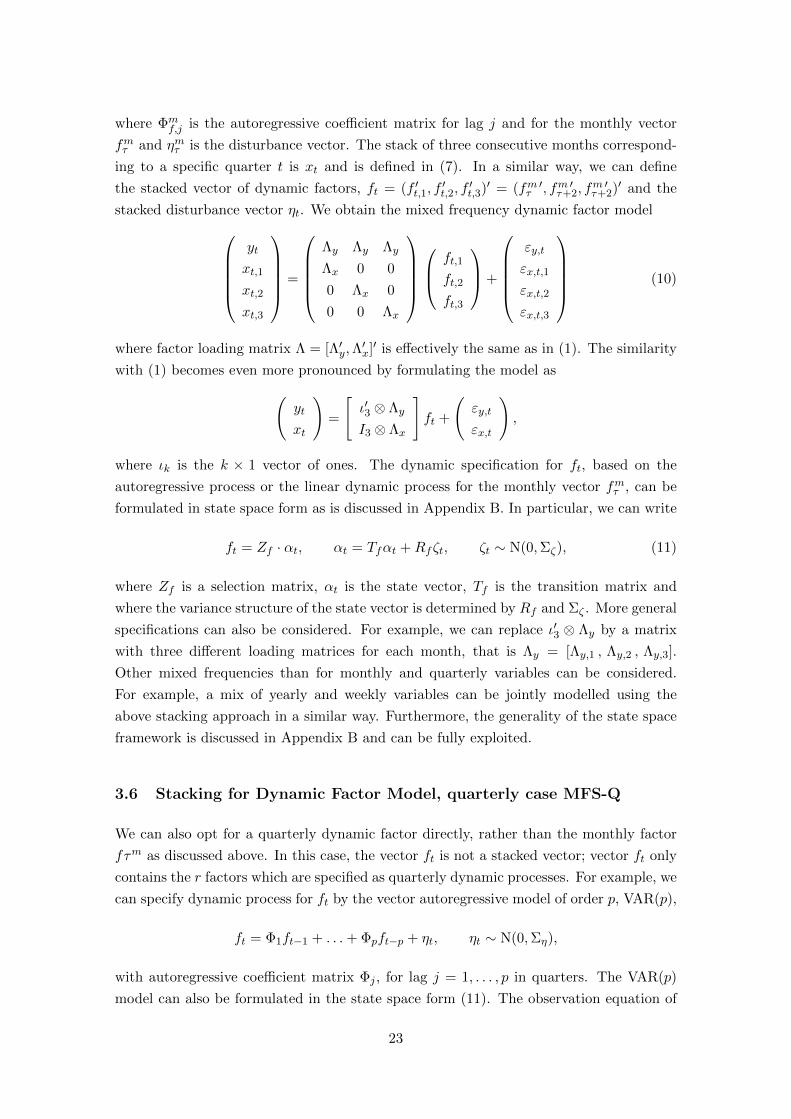
where Φmf,j is the autoregressive coefficient matrix for lag j and for the monthly vector

fmτ and ηmτ is the disturbance vector. The stack of three consecutive months correspond-

ing to a specific quarter t is xt and is defined in (7). In a similar way, we can define

the stacked vector of dynamic factors, ft = (f ′t,1, f′t,2, f

′t,3)′ = (fm ′τ , fm ′τ+2, f

m ′τ+2)′ and the

stacked disturbance vector ηt. We obtain the mixed frequency dynamic factor modelyt

xt,1

xt,2

xt,3

=

Λy Λy Λy

Λx 0 0

0 Λx 0

0 0 Λx

ft,1

ft,2

ft,3

+

εy,t

εx,t,1

εx,t,2

εx,t,3

(10)

where factor loading matrix Λ = [Λ′y,Λ′x]′ is effectively the same as in (1). The similarity

with (1) becomes even more pronounced by formulating the model as(yt

xt

)=

[ι′3 ⊗ Λy

I3 ⊗ Λx

]ft +

(εy,t

εx,t

),

where ιk is the k × 1 vector of ones. The dynamic specification for ft, based on the

autoregressive process or the linear dynamic process for the monthly vector fmτ , can be

formulated in state space form as is discussed in Appendix B. In particular, we can write

ft = Zf · αt, αt = Tfαt +Rfζt, ζt ∼ N(0,Σζ), (11)

where Zf is a selection matrix, αt is the state vector, Tf is the transition matrix and

where the variance structure of the state vector is determined by Rf and Σζ . More general

specifications can also be considered. For example, we can replace ι′3 ⊗ Λy by a matrix

with three different loading matrices for each month, that is Λy = [Λy,1 , Λy,2 , Λy,3].

Other mixed frequencies than for monthly and quarterly variables can be considered.

For example, a mix of yearly and weekly variables can be jointly modelled using the

above stacking approach in a similar way. Furthermore, the generality of the state space

framework is discussed in Appendix B and can be fully exploited.

3.6 Stacking for Dynamic Factor Model, quarterly case MFS-Q

We can also opt for a quarterly dynamic factor directly, rather than the monthly factor

fτm as discussed above. In this case, the vector ft is not a stacked vector; vector ft only

contains the r factors which are specified as quarterly dynamic processes. For example, we

can specify dynamic process for ft by the vector autoregressive model of order p, VAR(p),

ft = Φ1ft−1 + . . .+ Φpft−p + ηt, ηt ∼ N(0,Ση),

with autoregressive coefficient matrix Φj , for lag j = 1, . . . , p in quarters. The VAR(p)

model can also be formulated in the state space form (11). The observation equation of

23

the dynamic factor model for quarterly factors is then simply given by(yt

xt

)=

[Λy

ι3 ⊗ Λx

]ft +

(εy,t

εx,t

), (12)

In this case we only have one value for ft for each quarter, for all three months.

4 Empirical Study: forecasting U.S. GDP growth

4.1 Design of study

In our empirical study, we investigate the forecasting performances of our proposed mod-

els with their parameters estimated by weighted maximum likelihood. We focus on the

forecasting of U.S. GDP growth and adopt the standard database of Stock and Watson

(2005) that consists of 132 macroeconomic variables. This will facilitate the comparisons

with other empirical studies. We consider four different dynamic factor model (DFM)

specifications together with one benchmark model. The four DFMs differ in their treat-

ment of mixed frequency data. Our first model (mixed frequency interpolation, MFI) is

based on the model of Mariano and Murasawa (2003) which is formulated in a monthly

frequency. The key variable GDP growth has a quarterly frequency and is incorporated

in the model by having missing values for the months that the new GDP value is not

yet available. The remaining three models are formulated in the quarterly frequency.

The second model (average, MFA) simply treats all variables as quarterly variables; three

consecutive monthly observations are averaged to obtain the quarterly value. The third

model (stacked with monthly factors, MFS-M) treats monthly variables as a three di-

mensional vector of quarterly observations, preserves their monthly dynamics, and has

the dynamic factors as monthly variables. The fourth model (stacked with quarterly

factors, MFS-Q) is the same as the MFS-M model but has the dynamic factors as quar-

terly variables. The details of the last three models are described in Section 3. All these

mixed frequency dynamic factor models are extended with idiosyncratic autoregressive

components for each variable in zt = (y′t, x′t)′ as in the model specification of Mariano

and Murasawa (2003). The benchmark model is the well-known Bridge model of Trehan

(1989). We assess the improvements in forecasting and nowcasting accuracy by adopting

the method of weighted maximum likelihood for different weights W ; see the discussion in

Section 2. We evaluate the forecasting and nowcasting accuracy for the various methods

and compare the results, in terms of mean squared error (MSE) and the Diebold-Mariano

(DM) test.

Our dynamic factor modeling framework is similar to the one proposed by Brauning

and Koopman (2014) where the high-dimensional vector of related variables is collapsed

to a smaller set of principal components. In particular, we have Ny = 1 for the variable of

interest, GDP growth, and Nx = 7 for the monthly principal components obtained from

the Stock and Watson (2005) data set. The seven principal components are computed

24

as the first principal component from seven different groups of variables in the data set.

The details are provided next.

4.2 Data

We adopt the dataset of Stock and Watson (2005) for the forecasting of quarterly U.S.

GDP. This data set includes 132 real economic indicators, which are observed at a monthly

frequency from January 1960 to December 2009. The out-of-sample forecasting period

starts from January 2000 and ends at December 2009. We construct seven principal

components that correspond to the highest eigenvalue of the sample covariance matrix

of variables from seven different subsets of the data set. Each subset correspond to a

category of economic indicators; see the list of categories in Table 5. All the data are

transformed and demeaned so that no intercept coefficients are required in the model.

Detected outliers in each series are replaced by their median value of the previous five

observations; here we follow Stock and Watson (2005).

Indicator Description Frequency

Variable of interest ytDGP U.S. Real GDP (billions of chained 1996) Q

Related variables xtOUT First PC from category ”Real output and income”, 18 variables MEMP First PC from ”Employment and hours”, 30 variables MRTS First PC from ”Real retail, manufacturing and trade sales”, 2 variables MPCE Consumption, 1 variable MHHS First PC from ”Housing starts and sales”, 10 variables MORD First PC from ”Inventories and Orders”, 10 variables) MOTH First PC from category ”Other”, including stock prices, exchange rates, M

interest rates, money and credit, etc., 61 variables

Table 5: Data definitions. This table presents the definitions of all the quarterly, monthlyand semi-monthly variables that are used in our empirical study. Entries in the thirdcolumn present the frequency of the series: monthly(M) and quarterly(Q). The principalcomponent is referred to as PC.

4.3 Empirical results

We compare the forecast accuracies based on the mean square error (MSE). The sample

period from quarter 1, 2000 to quarter 4, 2009 (2000Q1-2009Q4) is used to evaluate the

forecasting performance. The forecasts are calculated using a rolling window of 20 years

of data to estimate the parameters. We evaluate both the nowcasting (h = 1, 2) and the

forecasting (h = 3, 6, 9, 12) performance of all the competing models. The forecasts are

calculated at a monthly frequency. When h = 1, the values of xt are known until the first

two months of the quarter that is to be forecasted. When h = 2, only the first month

of the quarter that we want to forecast is observed. When h = 3, we are forecasting one

quarter ahead, no observations are available for the quarter that we forecast. All values

25

until the previous quarter are observed. Similarly, when h = 6, 9, 12 we are forecasting

two, three and four quarters ahead respectively. In the MFA model, there are no monthly

dynamics, so it is only possible to forecast at h = 3, 6, 9, 12. The single common factor ft is

specified as an AR(1) process while all idiosyncratic factors are taken as AR(2) processes

for all models. Finally, for each model, the factor loading for the quarterly GDP growth

equation is set to the unity value for identification purposes.

We also evaluate the forecasting performance of MSF-M and MSF-Q using the weighted

maximum likelihood (WML) method. A cross validation analysis is implemented as fol-

lows. First, the WML parameter, W , is estimated using forecasting period 1980Q1-

1999Q4. The in-sample results are based on this estimation sample. For the estimated

W , we compute the forecasts of the period 2000Q1-2009Q4 and the out-of-sample forecasts

can be evaluated for all time periods.

h = 1 h = 2 h = 3 h = 6 h = 9 h = 12

MLBM 1.000 1.000 1.000 1.000 1.000 1.000

(1.000) (1.000) (1.000) (1.000) (1.000) (1.000)MFI 1.065 1.136 1.044 1.069 1.040 1.013

(0.672) (0.915) (0.692) (0.890) (0.761) (0.650)MFS-M 1.221 1.152 0.968 0.992 1.029 1.001

(0.975) (0.942) (0.210) (0.401) (0.856) (0.518)MFS-Q 1.022 0.973 0.916 0.993 1.070 1.040

(0.607) (0.380) (0.147) (0.455) (0.877) (0.749)MFA 0.981 0.970 1.004 0.990

(0.317) (0.142) (0.549) (0.328)

WMLMFS-M 1.221 1.152 0.968 0.992 1.029 1.001

(0.975) (0.942) (0.210) (0.401) (0.856) (0.518)MFS-Q 0.984 0.943 0.918* 0.993 0.994 1.015

(0.434) (0.294) (0.080) (0.439) (0.426) (0.719)

Table 6: Forecasting comparisons for the quarterly US DGP growth rate from 2000Q1 till2009Q4 at forecasting horizon h = 1, 2, 3, 6, 9, 12. We present the forecast RMSE ratiosof the competing models relative to the benchmark Bridge model (BM). We consider fourdynamic factor models as the competing models, which are mixed frequency Interpolation(MFI), mixed frequency stacking with monthly factors (MFS-M), mixed frequency stack-ing with quarterly factors (MFS-Q), and mixed frequency aggregation (MFA). All resultsare based on parameter estimates obtained form the 20-year rolling window starting from1980Q1. For each forecasting horizon the most accurate model is highlighted.

The forecasting results for the four mixed frequency dynamic factor models are com-

pared with the benchmark model in the first panel of Table 6. The MFS-Q model provides

the most accurate forecasts for the GDP growth rate among the dynamic factor models

when nowcasting and at the forecasting horizon h = 3. The accuracy is higher than

the original MFI model for all forecasting horizons. The quarterly MFA model is more

accurate for forecasts made at longer horizons, for h = 6, 9, 12. Furthermore, the MFS-Q

26

model is more accurate than the original MFI model for these forecast horizons. When

we further take into account the benchmark Bridge model, we find that the forecasts of

the Bridge model are most accurate at h = 0 and h = 9.

We adopt the Diebold-Mariano (DM) test to verify whether forecast accuracy of dy-

namic factor models are significantly different from the benchmark. The p values of the

DM test are also presented in Table 6. Although the MSE ratios for the dynamic factor

models are smaller than unity at the different forecasting horizons, none of these models

are significantly better than the benchmark, for any horizon and at the 10% level. For ex-

ample, MFS-M model has a smaller MSE than the benchmark model at horizon h = 3, 6

but the p values of the DM test has larger values than 0.1. The MFS-Q model has a

smaller MSE than the benchmark at horizon h = 2, 3, 6 but the p values of the DM test

are larger; only at h = 3 the p value is close to 0.1.

h = 1 h = 2 h = 3 h = 6 h = 9 h = 12

MFS-Q1 1.00000 1.00000 1.00000 1.00000 1.00000 1.000002 0.81878 0.82198 0.91035 0.94619 0.93689 0.945383 0.80361 0.79331 0.88796 0.93955 0.94181 0.933504 0.81675 0.78928 0.88118 0.93150 0.92853 0.935555 0.83421 0.78999 0.88394 0.93410 0.93216 0.936046 0.83999 0.78485 0.87975 0.93356 0.94094 0.937547 0.84836 0.78396 0.87840 0.94051 0.94526 0.934208 0.85676 0.78676 0.87727 0.94227 0.94674 0.936189 0.86989 0.79076 0.86854 0.94492 0.93127 0.9429510 0.87273 0.79033 0.87766 0.94750 0.94862 0.94201

MFS-M1 1.00000 1.00000 1.00000 1.00000 1.00000 1.000002 1.01600 1.01600 1.01600 1.01381 1.00225 0.999643 0.85002 0.83158 0.91551 1.00590 0.99455 1.017514 0.71480 0.73613 0.88738 1.00750 0.99112 1.031265 0.69002 0.70639 0.85165 0.96897 0.95040 0.999446 0.68837 0.70099 0.85427 0.98279 0.97446 1.005607 0.69169 0.70450 0.85604 0.98496 0.96951 1.021608 0.71637 0.73022 0.86932 0.99690 0.98272 1.016169 0.71382 0.71678 0.84706 0.99015 0.97717 1.0223210 0.70234 0.70515 0.85230 0.98552 0.98456 1.02290

Table 7: Forecasting comparisons for US GDP growth using MFS-Q and MFS-M, basedon ML and weighted ML (WML). The RMSE ratios of the forecasts are presented forthe quarterly observed US GDP growth based on the mixed frequency dynamic factormodel, at forecasting horizons h = 1, 2, 3, 6, 9, 12 using different W values in the WMLprocedure. The data sample period is from 1960Q1 till 1999Q4. For each forecastinghorizon the most accurate model is highlighted.

In the second panel of Table 6, we present the results for the weighted maximum

likelihood (WML) method applied to the MFS-M and MFS-Q models. We take different

integer values for W and determine its optimal value in the estimation sample. We adopt

27

effectively an cross validation approach. The value of W is selected using the sample from

1980Q1 until 1999Q4. The optimal value of W is adopted for the forecasting exercise;

see Table 7 for the MFS-Q and MFS-M models. The optimal weight at each forecasting

horizon is highlighted. We notice that the weight W is not limited to integer values

only. We have also investigated the MSE of the WML method for the out-of-sample

period. Some values of W around the optimal value found in Table 7 can still yield a

smaller MSE but the improvement is negligible and far from significant. Hence these

initial results already provide a clear picture of the usefullness of the WML method.

The out-of-sample forecast MSEs, for the period from 2000Q1 to 2009Q4, and based

on WML are presented in Table 6. They can be compared with the forecasting results

from the other dynamic factor and benchmark models. We may conclude that the WML

method improves the forecasting accuracy in the cross-validation sample but also provides

accurate out-of-sample forecasts in various cases. For example, the WML method leads

to a 3.7% improvement in MSE at h = 1, a 3.1% improvement at h = 2 and a 7.2%

improvement in MSE at h = 9 for MFS-Q model. For MFS-Q model at h = 3, the

standard ML method does not lead to a smaller MSE, but when applying WML method,

the MFS-Q model is significantly better than the benchmark at 10% confidence level.

We have shown that our stacking approach can treat mixed frequency data sets in

a standard fashion. The WML method is able to produce more accurate forecasts for

shorter forecast horizons.

5 Conclusions

This paper has introduced a novel weighted maximum likelihood (WML) estimation pro-

cedure for a class of mixed frequency dynamic factor models. The WML introduces a

variable-specific weight in the likelihood function to let some variable equations be of more

importance during the estimation process. We have derived the asymptotic properties of

the weighted ML estimator and have provided an information-theoretic characterization

of the WML estimator based on the Kullback-Leibler divergence. Furthermore, we have

proposed a cross-validation method to estimate the weights that optimize the forecasting

performance of the model and an F -statistic to test the statistical significance of the im-

provements in forecasting accuracy. A Monte Carlo study is carried out to investigate the

finite-sample behavior of the WML estimator; it highlights its good performance. Further-

more we have shown that the low frequency representation of high frequency variables in

a dynamic factor model provides a computational efficient treatment of mixed frequency

data. The representation is flexible and can allow for low and high frequency factors. The

presented illustration shows that our solutions lead to empirically relevant improvements

in nowcasting and forecasting of GDP growth. We expect that our proposed solutions

also have consequences in other applications and in other modeling frameworks.

28

References

Baffigi, A., R. Golinelli, and G. Parigi (2004). Bridge models to forecast the euro area

gdp. International Journal of Forecasting 20, 447–460.

Bai, J., E. Ghysels, and J. H. Wright (2011). State space models and midas regressions.

Working paper.

Banbura, M., D. Giannone, M. Modugno, and L. Reichlin (2013). Now-casting and

the real-time data flow. In G. Elliott and A. Timmermann (Eds.), Handbook of

Economic Forecasting, Volume 2, pp. 195–237. Elsevier.

Banbura, M. and M. Modugno (2014). Maximum Likelihood Estimation Of Factor

Models On Datasets With Arbitrary Pattern Of Missing Data. Journal of Applied

Econometrics 29 (1), 133–160.

Billingsley, P. (1961). The lindeberg-levy theorem for martingales. Proceedings of the

American Mathematical Society 12 (5), 788–792.

Bittanti, S. and P. Colaneri (2000). Invariant representations of discrete-time periodic

systems. Automatica 36 (12), 1777 – 1793.

Bittanti, S. and P. Colaneri (2009). Periodic Systems: Filtering and Control. Springer-

Verlag.

Blasques, F., S. J. Koopman, and A. Lucas (2014). Maximum likelihood estimation for

generalized autoregressive score models. Technical Report 14-029/III, Tinbergen

Institute Discussion Paper.

Bougerol, P. (1993). Kalman filtering with random coefficients and contractions. SIAM

Journal on Control and Optimization 31 (4), 942–959.

Brauning, F. and S. J. Koopman (2014). Forecasting macroeconomic variables using

collapsed dynamic factor analysis. International Journal of Forecasting 30 (3), 572–

584.

Chen, W., B. D. Anderson, M. Deistler, and A. Filler (2012). Properties of blocked

linear systems. Automatica 48 (10), 2520–2525.

Clark, T. E. and M. W. McCracken (2001, November). Tests of equal forecast accuracy

and encompassing for nested models. Journal of Econometrics 105 (1), 85–110.

Clark, T. E. and M. W. McCracken (2015). Nested forecast model comparisons: A new

approach to testing equal accuracy. Journal of Econometrics 186 (1), 160–177.

Diebold, F. X. (2012, September). Comparing Predictive Accuracy, Twenty Years

Later: A Personal Perspective on the Use and Abuse of Diebold-Mariano Tests.

NBER Working Papers 18391, National Bureau of Economic Research, Inc.

Diebold, F. X. and R. S. Mariano (1995). Comparing predictive accuracy. JBES 13 (3),

253–63.

29

Doz, C., D. Giannone, and L. Reichlin (2011). A two-step estimator for large ap-

proximate dynamic factor models based on Kalman filtering. Journal of Economet-

rics 164 (1), 188–205.

Durbin, J. and S. J. Koopman (2012). Time Series Analysis by State Space Methods.

Oxford: Oxford University Press.

Eguchi, S. and J. Copas (1998). A class of local likelihood methods and near-parametric

asymptotics. Journal of the Royal Statistical Society: Series B (Statistical Method-

ology) 60 (4), 709–724.

Engle, R. F. and M. W. Watson (1981). A one-factor multivariate time series model

of metropolitan wage rates. Journal of the American Statistical Association 76,

774–81.

Foroni, C., P. Gurin, and M. Marcellino (2015). Markov-switching mixed-frequency

VAR models. International Journal of Forecasting 31 (3), 692 – 711.

Foroni, C., M. Marcellino, and C. Schumacher (2015). Unrestricted mixed data sam-

pling (MIDAS): MIDAS regressions with unrestricted lag polynomials. Journal of

the Royal Statistical Society, Series A 178, 57–82.

Gallant, R. and H. White (1988). A Unified Theory of Estimation and Inference for

Nonlinear Dynamic Models. Cambridge University Press.

Ghysels, E. (2012). Macroeconomics and the Reality of Mixed Frequency Data.

Ghysels, E., J. B. Hill, and K. Motegi (2015). Testing for granger causality with mixed

frequency data. Journal of Econometrics, forthcoming.

Ghysels, E., P. Santa-Clara, and R. Valkanov (2006). Predicting volatility: getting

the most out of return data sampled at different frequencies. Journal of Economet-

rics 131, 59–95.

Giacomini, R. and H. White (2006, November). Tests of Conditional Predictive Ability.

Econometrica 74 (6), 1545–1578.

Giannone, D., L. Reichlin, and D. Small (2008). Nowcasting: the real-time informa-

tional content of macroeconomic data. Journal of Monetary Economics 55 (4), 665–

676.

Golinelli, R. G. and Parigi (2007). The use of monthly indicators to forecast quarterly

gdp in the short-run: An application to the g7 countries. Journal of Forecasting 26,

77–94.

Harvey, A. C. (1989). Forecasting, Structural Time Series Models and the Kalman

Filter. Cambridge: Cambridge University Press.

Hu, F. and J. Zidek (1997). The relevance weighted likelihood. Unpublished.

Jungbacker, B. and S. J. Koopman (2015). Likelihood-based dynamic factor analysis

for measurement and forecasting. Econometrics Journal 18, C1–C21.

30

Koopman, S. J. and J. Durbin (2000). Fast filtering and smoothing for multivariate

state space models. Journal of Time Series Analysis 21, 281–96.

Krengel, U. (1985). Ergodic theorems. Berlin: De Gruyter studies in Mathematics.

Kuzin, V., M. Marcellino, and C. Schumacher (2011). Midas vs. mixed-frequency var:

Nowcasting gdp in the euro area. International Journal of Forecasting 27 (2), 529–

542.

Marcellino, M., A. Carriero, and T. E. Clark (2014). Real-Time nowcasting with a

Bayesian mixed frequency model with stochastic volatility. Working paper.

Marcellino, M., J. H. Stock, and M. Watson (2003). Macroeconomic forecasting in

the euro area: country specific versus euro wide information. European Economic

Review 47, 1–18.

Mariano, R. and Y. Murasawa (2003). A new coincident index of business cycles based

on monthly and quarterly series. Journal of Applied Econometrics 18, 427–443.

Markatou, M., A. Basu, and B. G. Lindsay (1997). Weighted likelihood estimating

equations: The discrete case with applications to logistic regression. Journal of

Statistical Planning and Inference 57 (2), 215–232.

Markatou, M., A. Basu, and B. G. Lindsay (1998). Weighted likelihood equations with

bootstrap root search. Journal of the American Statistical Association 93 (442),

740–750.

Mehra, R. (1970). On the identification of variances and adaptive kalman filtering.

IEEE Transactions on Automatic Control 15 (2).

Mittnik, S. and P. A. Zadrozny (2005). Forecasting quarterly german gdp at monthly

intervals using monthly ifo business conditions data. In J.-E. Sturm and T. Wollmer-

shauser (Eds.), Ifo survey data in business cycle and monetary policy analysis, pp.

19–48. Heidelberg: Physica-Verlag.

Quah, D. and T. J. Sargent (1993). A dynamic index model for large cross sections. In

J. H. Stock and M. Watson (Eds.), Business cycles, indicators and forecasting, pp.

285–306. Chicago: University of Chicago Press.

Rao, R. R. (1962). Relations between Weak and Uniform Convergence of Measures with

Applications. The Annals of Mathematical Statistics 33 (2), 659–680.

Runstler, G., K. Barhoumi, S. Benk, R. Cristadoro, A. den Reijer, A. Jakaitiene,

P. Jelonek, A. Rua, K. Ruth, and C. V. Nieuwenhuyze (2009). Short-term forecast-

ing of GDP using large datasets: a pseudo real-time forecast evaluation exercise.

Journal of Forecasting 28 (7), 595–611.

Schorfheide, F. and D. Song (2013). Real-time forecasting with a mixed-frequency var.

NBER Working Papers 19712. Working paper.

31

Schumacher, C. and J. Breitung (2008). Real-time forecasting of German GDP based

on a large factor model with monthly and quarterly data. International Journal of

Forecasting 24 (3), 386–398.

Staniswalis, J. G. (1989). The kernel estimate of a regression function in likelihood-

based models. Journal of the American Statistical Association 84 (405), 276–283.

Stock, J. H. and M. Watson (2002). Macroeconomic forecasting using diffusion indexes.

Journal of Business and Economic Statist. 20, 147–62.

Stock, J. H. and M. Watson (2005). Implications of dynamic factor models for var

analysis. Discussion paper.

Straumann, D. and T. Mikosch (2006). Quasi-maximum-likelihood estimation in con-

ditionally heteroeskedastic time series: A stochastic recurrence equations approach.

The Annals of Statistics 34 (5), 2449–2495.

Tibshirani, R. and T. Hastie (1987). Local likelihood estimation. Journal of the Amer-

ican Statistical Association 82 (398), 559–567.

Trehan, B. (1989). Forecasting growth in current quarter real gnp. Federal Reserve

Bank of San Francisco, Economic Review Winter, 39–52.

van der Vaart, A. W. (2000, June). Asymptotic Statistics (Cambridge Series in Statis-

tical and Probabilistic Mathematics). Cambridge University Press.

Wang, X., C. van Eeden, and J. V. Zidek (2004). Asymptotic properties of max-

imum weighted likelihood estimators. Journal of Statistical Planning and Infer-

ence 119 (1), 37–54.

Wang, X. and J. V. Zidek (2005). Selecting likelihood weights by cross-validation. The

Annals of Statistics 33 (2), 463–500.

Watson, M. W. and R. F. Engle (1983). Alternative algorithms for the estimation of

dynamic factor, MIMIC and varying coefficient regression. Journal of Economet-

rics 23, 385–400.

West, K. D. (1996, September). Asymptotic Inference about Predictive Ability. Econo-

metrica 64 (5), 1067–84.

White, H. (1994). Estimation, Inference and Specification Analysis. Cambridge Books.

Cambridge University Press.

Zadrozny, P. A. (1990). Estimating a multivariate ARMA model with mixed-frequency

data: An application to forecasting U.S. GNP at monthly intervals. Federal Reserve

Bank of Atlanta Working Paper Series No. 90-6.

32

Technical Appendix

Weighted Maximum Likelihood Estimator for

Mixed Frequency Dynamic Factor Models

Francisco Blasques, Siem Jan Koopman, Max Mallee and Zhaokun Zhang

VU University Amsterdam, Department of Econometrics

Tinbergen Institute Amsterdam

A Proofs of Theorems and Propositions

Proof of Proposition 1. Let ft(f∗1 )t∈N be generated according to (9) with initialization

f∗1 and ‖Tf‖ < 1, ‖Rf‖ < ∞ and ‖Σ2η‖ < ∞. Then by Theorem 3.1 in Bougerol (1993),

ft(f∗1 )t∈N converges to an SE sequence ftt∈Z satisfying E|ft|r < ∞ ∀ r. Uniqueness

of the limit SE sequence is obtained in Straumann and Mikosch (2006). Furthermore,

since ft is a linear Gaussian process with E|xt|r < ∞ ∀ r > 0. The bounds |βx| < ∞and 0 < σ2

ε < ∞, together with the iid Gaussian nature of the innovations εt ensure

that xt is SE and Gaussian with bounded moments of any order. Similarly, the bounds

|βy| < ∞ and 0 < σ2ζ < ∞ and the iid Gaussian nature of ζt ensure the SE linear

Gaussian nature of yt with E|yt|r <∞ ∀ r > 0.

Proof of Theorem 1. For every given w ∈ [0, 1], the random likelihood function LT (·, f∗1 )

is trivially almost surely continuous on Ψ. The compactness of Ψ implies by Weierstrass’

theorem that the arg max set is almost surely non-empty. As a result, ψT exists almost

surely ∀ T ∈ N. The continuity of the likelihood function in ft, xt and yt for every ψ ∈ Ψ

implies also measurability of the likelihood under the Borel σ-algebra. For every given

w ∈ [0, 1] the measurability of the WML estimator can now be obtained by application

of Theorem 2.11 of White (1994) or Lemma 2.1 and Theorem 2.2 in Gallant and White

(1988).

Proof of Theorem 2. The consistency of the WML estimator can be obtained by appealing

to the classical extremum estimation theory found e.g. in Theorem 3.4 of White (1994)

or Theorem 3.3 of Gallant and White (1988). In particular, for any weight w ∈ (0, 1] and

initialization f∗1 , the consistency ψT (w, f∗1 )a.s.→ ψ0 follows from the uniform convergence

of the weighted likelihood

supψ∈Ψ|LT (ψ,w, f∗1 )− L∞(ψ,w)| a.s.→ 0 ∀ f∗1 ∈ R+ as T →∞, (13)

and the identifiable uniqueness of the true parameter ψ0 ∈ Ψ defined e.g. in White (1994).

33

To establish the uniform convergence of LT (ψ,w, f∗1 ) we use the norm sub-additivity

inequality

supψ∈Ψ|LT (ψ,w, f∗1 )− L∞(ψ,w)| ≤ sup

ψ∈Ψ|LT (ψ,w, f∗1 )− LT (ψ,w)|+ sup

ψ∈Ψ|LT (ψ,w)− L∞(ψ,w)|

where LT (ψ,w) denotes the likelihood evaluated at the filtered ft(ψ) starting in the

infinite past. The term

supψ∈Ψ|LT (ψ,w, f∗1 )− LT (ψ,w)|

vanishes by the assumption that ‖ft(ψ,w, f∗1 )− ft(ψ)‖ a.s.→ 0, the continuity of the likeli-

hood function and the continuous mapping theorem.

The ergodic theorem for separable Banach spaces of Rao (1962) ensures that

supψ∈Ψ|LT (ψ,w)− L∞(ψ,w)| a.s.→ 0

(see also Theorem 2.7 in Straumann and Mikosch (2006)) for the sequence LT (·, w) of

points in C(Ψ,R) under:

(i) the SE nature of LT (·, w)T∈Z which is ensured by SE nature of ftt∈Z, xtt∈Zand ytT∈Z, by the continuity of and Proposition 4.3 in Krengel (1985);

(ii) the moment bound E supψ∈Ψ |`t(ψ,w)| <∞ ensured by the Gaussian log likelihood

under the bounded second moment of ft, xt and yt.

The identifiable uniqueness of the true parameter ψ0 ∈ Ψ, typically defined as

supψ:‖ψ−ψ0‖>ε

`∞(ψ,w) < `∞(ψ0, w) ∀ ε > 0

is ensured by the uniqueness of ψ0, the compactness of Ψ, and the continuity of E`t(ψ,w)

on Ψ, which is obtained through the continuity of LT on Ψ for every T ∈ N and the

uniform convergence of the likelihood; see e.g. White (1994). The uniqueness of ψ0 as

the maximizer L∞(·, w) for any w ∈ (0, 1] is ensured by Theorem 3 which shows that the

maximizer L∞(ψ0, w) = 0 if and only if L∞(ψ0, 1) = 0.

Proof of Theorem 3. The consistency statement follows by the same steps as the proof of

Theorem 2 with the exception that the SE nature of yt is assumed rather than derived

through Proposition 1.

Let zt denote a dz-variate random vector with joint density p(zt). Furthermore, con-

sider a family of parametric joint densities indexed by the parameter vector ψ, defined as

Q(Ψ) := q(zt;ψ), ψ ∈ Ψ. Note that it is possible but not necessary that p(zt) ∈ Q(Ψ).

If ψ∗0(1) is the pseudo-true parameter that maximizes the limit log likelihood function

ψ∗0 := arg maxψ∈Ψ

E0 log q(zt;ψ),

34

then it is well known that ψ∗0 also minimizes the the Kullback–Leibler divergence KL(p, q(·;ψ)

)between p(zt) and q(zt;ψ) because

arg maxψ∈Ψ

E0 log q(zt;ψ) = arg minψ∈Ψ

E0 log p(zt)− E0 log q(zt;ψ) = arg minψ∈Ψ

KL(p, q(·;ψ)

).

Let now the joint density q(xt;ψ) be factorized into

q1(z1,t|z2:dz ,t;ψ0)× q2(z2:dz ,t;ψ0) := q1(z1,t|z2,t, ..., zdz ,t;ψ0)× q2(z2,t, z3,t, ..., zdz ,t;ψ0)

and define ψ∗0(w) as the pseudo-true parameter that maximizes the weighted limit log

likelihood function

ψ∗0(w) := arg maxψ∈Ψ

E0 log q1(z1,t|z2:dz ,t;ψ) + w logE0q2(z2:dz ,t;ψ).

Then it follows naturally that ψ∗0(w) is the minimizer of the weighted average of KL

divergences

ψ∗0(w) = arg minψ∈Ψ

KL(q1, p1) + wKL(q2, p2)

because

arg maxψ∈Ψ

[E0 log q1(z1,t|z2:dz ,t;ψ) + w logE0q2(z2:dz ,t;ψ)

]= arg max

ψ∈Ψ

[E0 log q1(z1,t|z2:dz ,t;ψ)− E0 log p1(z1,t|z2:dz ,t)

+ w logE0q2(z2:dz ,t;ψ)− w logE0p2(z2:dz ,t)]

= arg minψ∈Ψ

[E0 log p1(z1,t|z2:dz ,t)− E0 log q1(z1,t|z2:dz ,t;ψ)

+ w(

logE0p2(z2:dz ,t)− logE0q2(z2:dz ,t;ψ))]

= arg minψ∈Ψ

[KL(q1(·;ψ), p1) + wKL(q2(·;ψ), p2)

].

Clearly, if w = 1, then we obtain the usual ML pseudo-true parameter since

ψ∗0(1) = arg minψ∈Ψ

KL(q1(·;ψ), p1) + KL(q2(·;ψ), p2) = arg minψ∈Ψ

KL(q(·;ψ), p).

For w = 0 we obtain the ML estimator for the conditional model

ψ∗0(0) = arg minψ∈Ψ

KL(q1(·;ψ), p1)

Finally, it is also clear that the transformed KL divergence TKL(q, p) := KL(q1(·;ψ), p1)+

wKL(q2(·;ψ), p2) satisfies

KL(q1(·;ψ), p(·;ψ)) ≤ TKL(q(·;ψ), p) ≤ KL(q(·;ψ), p)

35

and that TKL(q(·;ψ), p) is a pre-metric for any w ∈ (0, 1] as it inherits positivity TKL(q(·;ψ), p) ≥0 from the positivity of the KL divergence, and satisfies also the identity of indiscernibles

since

TKL(q(·;ψ), p) = KL(q1(·;ψ), p1) + wKL(q2(·;ψ), p2) = 0

if and only if q1(·;ψ) = p1 and q2(·;ψ) = p2, and hence, if and only if q(·;ψ) = p.

Proof of Theorem 4. Asymptotic normality of the WML estimator can be obtained by

verifying the conditions of Theorem 6.2 of White (1994):

(i) ψT (f∗1 , w)a.s.→ ψ0 ∈ int(Ψ);

(ii) LT (·, w, f∗1 ) ∈ C2(Ψ) a.s.;

(iii)√TL′T

(ψ0, w, f

∗1 , df

∗1)

d→ N(0,J (ψ0, w));

(iv) supψ∈Ψ

∥∥L′′T (ψ,w, f∗1 , df∗1,

˜ddf∗1)− `′′∞(ψ,w)

∥∥ a.s.→ 0;

(v) `′′∞(ψ,w) = E`′′t (ψ,w) = I(ψ,w) is non-singular

Conditions (i) and (ii) follow naturally from Theorem 2, the additional assumption

that ψ0 ∈ int(Ψ) and the differentiability of the Gaussian likelihood.

Condition (iii) follows by the asymptotic SE nature of the score `′t(ψ,w, f∗1 , df∗1)

which is implied by the SE nature of xt and yt, and the asymptotic SE nature of

the filtered sequence ft(ψ, f∗1 ) and its derivative df t(ψ, df∗1). Since the limit score

sequence `′t(ψ,w) is SE we can apply the CLT for SE martingales in Billingsley (1961)

to obtain √TL′T

(ψ0, w)

d→ N(0,J (ψ0, w))

as T →∞, (14)

where J (ψ0, w) = E(`′t(ψ0, w)`′t

(ψ0, w)>) < ∞. By Theorem 18.10[iv] in van der Vaart

(2000) it thus follows that

√TL′T

(ψ0, w, f

∗1 , df

∗1)

d→ N(0,J (ψ0, w))

as T →∞,

as long as

‖L′T(ψ0, w, f

∗1 , df

∗1)− L′T

(ψ0, w)‖ e.a.s.→ 0 as T →∞ (15)

since (15) ensures√T‖L′T

(ψ0, w, f

∗1 , df

∗1) − L′T

(ψ0, w)‖ a.s.→ 0 as T → ∞. The e.a.s. con-

vergence in (15) follows from

|ft(ψ0, w, f∗1 )− ft(ψ0, w)| e.a.s.→ 0

and

‖df t(ψ0, df∗1)− df t(ψ0)‖ e.a.s.→ 0.

Furthermore, since the score of the weighted likelihood is differentiable, we can use the

36

mean-value theorem to obtain

‖L′T(ψ0, w, f

∗1 , df

∗1)− L′T

(ψ0, w)‖ ≤

∑j

∣∣dL′T ∣∣∣∣df j,t(ψ0, df∗1)− df j,t(ψ0)

∣∣, (16)

where df j,t(ψ0, df∗1) denotes the j-th element of df t(ψ0, df

∗1), and dL′T denotes the deriva-

tive ∂L′T(ψ0, w, f

∗1 , df

∗1)/∂df j evaluated at some appropriate point between df j,t(ψ0, df

∗1)

and df j,t(ψ0). The bounded moments of the weighted likelihood derivatives and the

e.a.s. convergence of the filtered process and its derivatives yield

‖L′T(ψ0, w, f

∗1 , df

∗1)− L′T

(ψ0, w)‖ =

∑j

Op(1)oe.a.s(1) = oe.a.s.(1). (17)

Condition (iv) follows by noting that

supψ∈Ψ‖L′′T

(ψ,w, f∗1 , df

∗1,

˜ddf∗1)− L′′∞

(ψ,w) ≤ sup

ψ∈Ψ‖L′′T

(ψ,w, f∗1 , df

∗1,

˜ddf∗1)− L′′T

(ψ,w)‖

+ supψ∈Ψ‖L′′T

(ψ,w)− L′′∞

(ψ,w)‖.

(18)

Clearly, supψ∈Ψ ‖L′′T(ψ,w, f∗1 , df

∗1,

˜ddf∗1)− L′′T

(ψ,w)‖0 as t→∞ by the continuous map-

ping theorem and the e.a.s. convergence of the filtered process and its derivatives, and

supψ∈Ψ ‖L′′T(ψ,w) − L′′∞

(ψ,w)‖ vanishes by a ULLN under the uniform moment bound

on the weighted likelihood E supψ∈Ψ ‖L′′t (ψ,w)‖ <∞.

Condition (v) is the uniqueness of ψ0 as a maximum of `′′∞(ψ,w) and ensures the

non-singularity of the limit weighted likelihood L′′∞(ψ,w) = EL′′t (ψ,w) = I(ψ,w).

Proof of Theorem 5. Follows the same steps as the proof of Theorem 4 ith the exception

that the required properties of xt and yt are directly assumed rather than derived

through Proposition 1.

B Low frequency formulations for autoregressions

B.1 Notation

In this Appendix we discuss the stacking approach similar to the one used by Ghysels

(2012) and Foroni, Marcellino, and Schumacher (2015). In the main paper we adopt the

stacking method to treat mixed frequency dynamic factor model within a state space

setting. But here we provide the details for the autoregressive model case for monthly

time series (high frequency) that can be represented by quarterly (low frequency) vectors

within a state space formulation. We use the notation xmτ for a variable x that is observed

on a monthly (m) basis with monthly time index τ . The observations of the time series

xmτ can be stacked into a quarterly (q) observed 3×1 vector xqt with quarterly time index

t

37

xqt =

xqt,1xqt,2xqt,3

=

xm3(t−1)+1

xm3(t−1)+2

xm3(t−1)+3

, (19)

where xqt,i is the i-th element of xqt with index t indicating the number of the quarter

of the observation and index i indicating the number of the month within the quarter;

we have t = 1, . . . , T , i = 1, 2, 3 and τ = 1, . . . , 3n, since each quarter consists of s = 3

months.

In a similar way, we can represent the monthly observations into yearly vectors. The

monthly observed series xmτ can be stacked into a yearly (y) observed 12 × 1 vector xytwith yearly time index t. We then have

xyt =

xyt,1xyt,2

...

xyt,12

=

xm12(t−1)+1

xm12(t−1)+2...

xm12(t−1)+12

, (20)

where xyt,i is the i-th element of xyt with the first t indicating the number of the year of

the observation and second index i indicating the number of the month within the year;

we have t = 1, . . . , T , i = 1, . . . , 12 and τ = 1, . . . , 12n, since each year consists of s = 12

months. Throughout this paper, we will use the superscripts m, q and y to indicate the

frequency of time series; we only use this notation where we deem it is necessary. When

a variable or vector has only one index, this index typically refers to the number of the

month, quarter or year of the observation. The second index refers to the number of the

month within the quarter or year of the observation.

B.2 Linear State Space Models

The general linear Gaussian state space model can be written in a variety of ways. In

this paper we adopt the notation used in Durbin and Koopman (2012), where the model

is given as

xt = Zαt + εt, εt ∼ NID (0, H) ,

αt+1 = Tαt +Rηt, ηt ∼ NID (0, Q) ,(21)

where xt is a k × 1 vector of observations called the observation vector and αt is an

unobserved m× 1 vector called the state vector. The system matrices Z, T , R, H and Q

are initially assumed to be known and the error terms εt and ηt are assumed to be serially

independent and independent of each other at all time points. In practice, some or all of

the matrices Z, T , R, H and Q will depend on elements of an unknown parameter vector

ψ.

In the state space model, the state vector αt cannot be observed directly and hence

we base the analysis on observations xt. These equations hold true for any frequency, as

38

long as the state vector has the same frequency as the observation vector. Therefore, we

do not use a superscript to indicate the frequency of the series, although we use these

mostly for low frequency models.

The initial state vector α1 is generated from N(a1, P1), independently of ε1, . . . , εn

and η1, . . . , ηn, where a1 and P1 are assumed known, although P1 may depend on the

parameter vector ψ.

B.3 Autoregressive Processes

We now adopt the stacking method in an autoregressive (AR) model setting. For brevity,

we illustrate the method using an AR(1). Illustrations with AR(p) models or higher

order p are provided in Appendix A. Detailed derivations for all models are provided in

the Technical Appendix.

Monthly observations from the AR(1) process xmτ = φxmτ−1 + εmτ are stacked into the

quarterly 3× 1 vector xqt of (19). The quarterly process of the stacked variable xqt is then

given by the vector autoregressive process

xqt = Txqt−1 +Rεqt (22)

with

T =

0 0 φ

0 0 φ2

0 0 φ3

, R =

1 0 0

φ 1 0

φ2 φ 1

, (23)

such that the variance matrix of the vector xqt , conditional on xqt−1, is equal to σ2εRR

′.

We notice that all three elements of xqt depend only on the last element of xqt−1 and on

the associating elements of the vector of disturbances εqt . The vector εqt is the result of

stacking the values of εmτ in similar fashion as in (19). The autoregressive process (22) is

equal to the linear Gaussian state space model (21) with state vector αt = xqt and with

system matrices T and R given by (23) and Z = I3, H = 0, Q = σ2ε and ηt = εqt .

B.4 AR(1) process with stacked observations

Consider the AR(1) process of the monthly (m) observed variable xmτ with monthly time

index τ

xmτ = φxmτ−1 + ετ , ετ ∼ NID(0, σ2

ε

)(24)

When the monthly observations of xmτ are stacked into the quarterly (q) 3× 1 vectors

xqt with quarterly time index t, then the equations of the AR(1) process for the stacked

observations can be written as

xqt,1 = φxqt−1,3 + εt,1, xqt,2 = φxqt,1 + εt,2, xqt,3 = φxqt,2 + εt,3 (25)

39

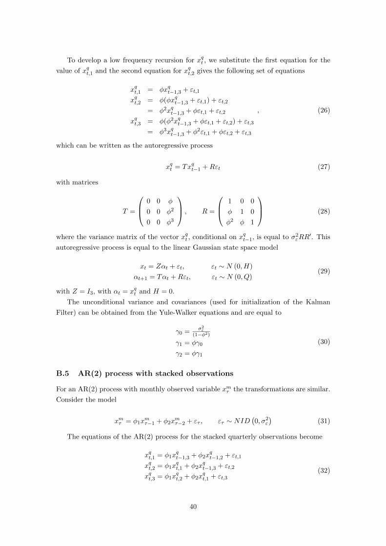
To develop a low frequency recursion for xqt , we substitute the first equation for the

value of xqt,1 and the second equation for xqt,2 gives the following set of equations

xqt,1 = φxqt−1,3 + εt,1

xqt,2 = φ(φxqt−1,3 + εt,1) + εt,2

= φ2xqt−1,3 + φεt,1 + εt,2

xqt,3 = φ(φ2xqt−1,3 + φεt,1 + εt,2) + εt,3

= φ3xqt−1,3 + φ2εt,1 + φεt,2 + εt,3

, (26)

which can be written as the autoregressive process

xqt = Txqt−1 +Rεt (27)

with matrices

T =

0 0 φ

0 0 φ2

0 0 φ3

, R =

1 0 0

φ 1 0

φ2 φ 1

(28)

where the variance matrix of the vector xqt , conditional on xqt−1, is equal to σ2εRR

′. This

autoregressive process is equal to the linear Gaussian state space model

xt = Zαt + εt, εt ∼ N (0, H)

αt+1 = Tαt +Rεt, εt ∼ N (0, Q)(29)

with Z = I3, with αt = xqt and H = 0.

The unconditional variance and covariances (used for initialization of the Kalman

Filter) can be obtained from the Yule-Walker equations and are equal to

γ0 = σ2ε

(1−φ2)

γ1 = φγ0

γ2 = φγ1

(30)


For an AR(2) process with monthly observed variable xmτ the transformations are similar.

Consider the model

xmτ = φ1xmτ−1 + φ2x

mτ−2 + ετ , ετ ∼ NID

(0, σ2

ε

)(31)

The equations of the AR(2) process for the stacked quarterly observations become

xqt,1 = φ1xqt−1,3 + φ2x

qt−1,2 + εt,1

xqt,2 = φ1xqt,1 + φ2x

qt−1,3 + εt,2


qt,1 + εt,3

(32)

40

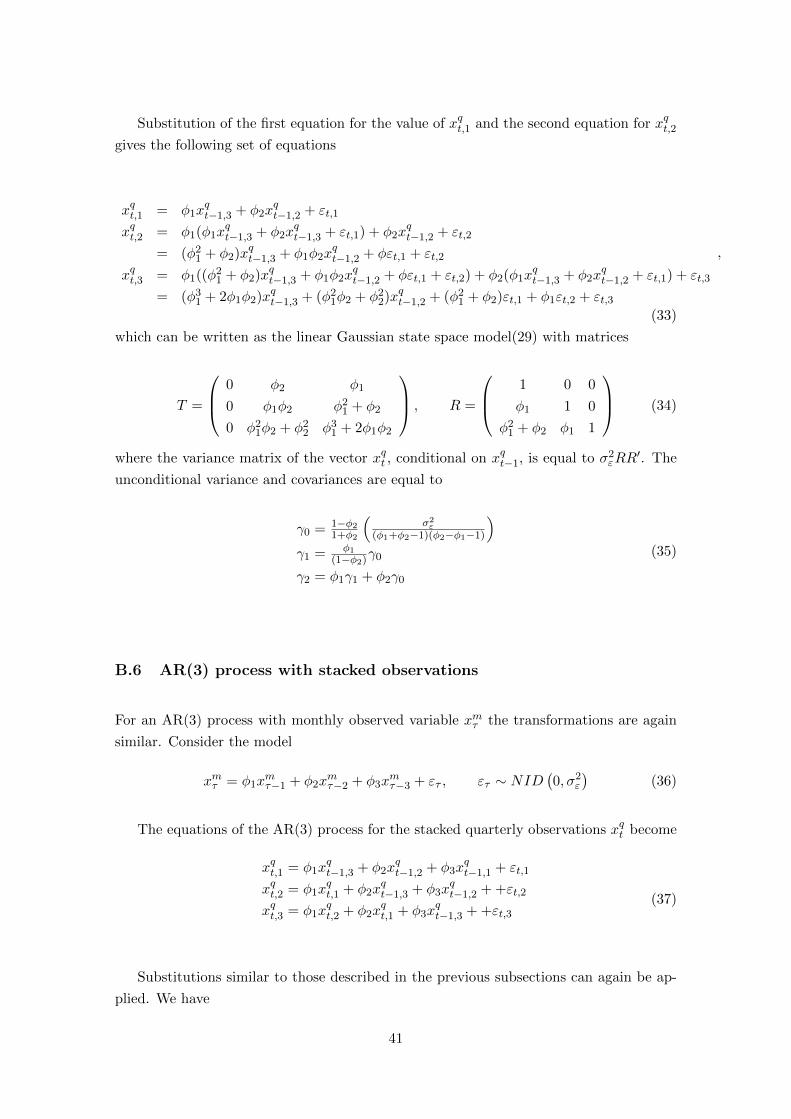
Substitution of the first equation for the value of xqt,1 and the second equation for xqt,2gives the following set of equations

xqt,1 = φ1xqt−1,3 + φ2x

qt−1,2 + εt,1

xqt,2 = φ1(φ1xqt−1,3 + φ2x

qt−1,3 + εt,1) + φ2x

qt−1,2 + εt,2

= (φ21 + φ2)xqt−1,3 + φ1φ2x

qt−1,2 + φεt,1 + εt,2

xqt,3 = φ1((φ21 + φ2)xqt−1,3 + φ1φ2x

qt−1,2 + φεt,1 + εt,2) + φ2(φ1x

qt−1,3 + φ2x

qt−1,2 + εt,1) + εt,3

= (φ31 + 2φ1φ2)xqt−1,3 + (φ2

1φ2 + φ22)xqt−1,2 + (φ2

1 + φ2)εt,1 + φ1εt,2 + εt,3

,

(33)

which can be written as the linear Gaussian state space model(29) with matrices

T =

0 φ2 φ1

0 φ1φ2 φ21 + φ2

0 φ21φ2 + φ2

2 φ31 + 2φ1φ2

, R =

1 0 0

φ1 1 0

φ21 + φ2 φ1 1

(34)

where the variance matrix of the vector xqt , conditional on xqt−1, is equal to σ2εRR

′. The

unconditional variance and covariances are equal to

γ0 = 1−φ21+φ2

(σ2ε

(φ1+φ2−1)(φ2−φ1−1)

)γ1 = φ1

(1−φ2)γ0

γ2 = φ1γ1 + φ2γ0

(35)


For an AR(3) process with monthly observed variable xmτ the transformations are again

similar. Consider the model

xmτ = φ1xmτ−1 + φ2x

mτ−2 + φ3x

mτ−3 + ετ , ετ ∼ NID

(0, σ2

ε

)(36)

The equations of the AR(3) process for the stacked quarterly observations xqt become

xqt,1 = φ1xqt−1,3 + φ2x

qt−1,2 + φ3x

qt−1,1 + εt,1


qt−1,3 + φ3x

qt−1,2 + +εt,2


qt,1 + φ3x

qt−1,3 + +εt,3

(37)

Substitutions similar to those described in the previous subsections can again be ap-

plied. We have

41

xqt,1 = φ1xqt−1,3 + φ2x

qt−1,2 + φ3x

qt−1,1 + εt,1


qt−1,3 + φ3x

qt−1,2 + εt,1

= φ1(φ1xqt−1,3 + φ2x

qt−1,2 + φ3x

qt−1,1 + εt,1) + φ2x

qt−1,3 + φ3x

qt−1,2 + εt,2

= (φ21 + φ2)xqt−1,3 + (φ1φ2 + φ3)xqt−1,2 + φ1φ3x

qt−1,1 + φεt,1 + εt,2


qt,1 + φ3x

qt−1,3 + εt,1

= φ1(φ1xqt−1,3 + φ2x

qt−1,2 + φ3x

qt−1,1 + εt,1)

+ φ2((φ21 + φ2)xqt−1,3 + (φ1φ2 + φ3)xqt−1,2 + φ1φ3x

qt−1,1 + φεt,1 + εt,2)

+ φ3xqt−1,3 + εt,2

= (φ31 + 2φ1φ2 + φ3)xqt−1,3 + (φ2

1φ2 + φ1φ3 + φ22)xqt−1,2

+ (φ21φ3 + φ2φ3)xqt−1,1 + φεt,1 + εt,2

, (38)

which can be written as the linear Gaussian state space model (29) for the quarterly

observed xqt with

T =

φ3 φ2 φ1

φ1φ3 φ1φ2 + φ3 φ21 + φ2

φ21φ3 + φ2φ3 φ2

1φ2 + φ1φ3 + φ22 φ3

1 + 2φ1φ2 + φ3

(39)

For the AR(3) process, R is the same matrix as for the AR(2) process and the variance

matrix of the vector xqt , conditional on xqt−1, is again equal to σ2εRR

′. The three values

of xqt now depend on all three observation of xqt−1 and on the 3× 1 vector of disturbances

εt. The unconditional variance and covariances are equal to

γ0 =σ2ε(1−φ2−φ1φ3−φ23)

(1−φ2−φ3−φ1)(1+φ2+φ3φ1−φ23)(1+φ3+φ1−φ2)

γ1 = (φ1+φ2φ3)γ0

(1−φ2−φ3φ1−φ23)

γ2 = φ1γ1 + φ2γ0 + φ3γ1

(40)

B.7 AR(p) process with stacked observations

For AR(p) processes of order p > 3 the state vector in (29) has to be extended with more

lags of xqt . For example, for the AR(4) process we would have αt =(xqt−1,3, x

qt,1, x

qt,3, x

qt,3

)′and the transition matrix becomes

T =

0 0 0 1

φ4 φ3 φ2 φ1

φ1φ4 φ1φ3 + φ4 φ1φ2 + φ3 φ21 + φ2

φ21φ4 + φ2φ4 φ2

1φ3 + φ2φ3 + φ1φ4 φ21φ2 + φ1φ3 + φ2

2 + φ4 φ31 + 2φ1φ2 + φ3

,

(41)

where the variance matrix of the process is defined as σ2εRR

′ with

42

R =

0 0 0 0

0 1 0 0

0 φ1 1 0

0 φ21 + φ2 φ1 1

, (42)

The unconditional variances and covariances can be obtained analytically using the

Yule-Walker equations, or by numerically solving the Algebraic Riccati Equation.

B.8 Computing times

Computing time (in seconds) State vector length

Monthly Quarterly Yearly Monthly Quarterly Yearlyp (n = 12k) (n = 4k) (n = 1k) (n = 12k) (n = 4k) (n = 1k)

1 10 13 61 1 3 122 11 16 67 2 3 123 26 18 76 3 3 124 41 27 85 4 4 125 59 40 92 5 5 126 83 56 100 6 6 127 106 73 108 7 7 128 129 90 116 8 8 129 154 111 124 9 9 1210 191 137 133 10 10 1211 226 162 139 11 11 1212 265 190 146 12 12 12

Table 8: Computing times. The left panel of this table presents the average computingtime (in seconds) that is required to evaluate the loglikelihood function for an AR(p)model of order p for a monthly time series xmτ that is generated by an AR(p) model.Three different approaches are used: treating the data as monthly observations, stackingthe data into quarterly 3 × 1 vectors and stacking the data into yearly 12 × 1 vectors.Each value represents the average over 10,000 simulation runs. For each value of p thefastest of the three approaches is highlighted. The right panel of this table presents thestate vector length for each scenario.

C Interpolation and Aggregation Approaches

Below we discuss the original solution by Mariano and Murasawa (2003) in treating mixed

frequency data; they analyze all series at the highest frequency. In this approach, artificial

missing values are introduced for the series that is observed at the lower frequency and

interpolation techniques are used to describe the dynamics of the unobserved ’latent’

monthly GDP growth. Furthermore, we explore a second approach where all series are

modeled at the lowest frequency by aggregating the high frequency series to quarterly

totals. In this approach, no artificial missing values are needed, but information about

43

the high frequency series is lost and the model does not allow the econometrician to

address high frequency dynamics.

C.1 Interpolation Approach

In the mixed frequency interpolation (MFI) approach, all series are treated at the highest

frequency, say as monthly time series. All variables are driven by one unobserved monthly

common factor fτ and by the idiosyncratic factors uτ and vτ . The variable quarterly yt

is observed every third month and has missing values for the first two months of every

quarter. Therefore, the data matrix has the following structure

[· · y3 · · y6 · . . . y3n

x1 x2 x3 x4 x5 x6 x7 . . . x3n

], (43)

where xτ is the k × 1 vector(x

(1)τ , . . . , x

(k)τ

)′and n is the number of quarters in the

sample period. Since in this approach all series are treated as monthly series, we choose

to drop the superscript m, in order to avoid cumbersome notation. The contemporaneous

and dynamic interactions between yτ and the vector of monthly observed variables xτ are

specified via the model

(ymτxτ

)=

(βyg (fτ )

βxfτ

)+

(g(uτ )

vτ

)+

(ξτ

ετ

)(44)

where ymτ is the latent monthly variable for y and for which we only have observations

available in the last month of each quarter, βy is a scalar coefficient, βx is a k × 1 vector

of coefficients, and

g(aτ ) =1

3aτ +

2

3aτ−1 + aτ−2 +

2

3aτ−3 +

1

3aτ−4 (45)

for τ = 1, . . . , 3n. The vector uτ is the stationary sequence of the idiosyncratic factor

for yτ and vτ is the stationary sequence of the vector of idiosyncratic factors for xτ and

consists of one value per month for each monthly observed variable x(i)τ .

The factors fτ , uτ and vτ are modeled as AR processes

fτ ∼ AR(pf ), uτ ∼ AR(pu), vτ ∼ AR(pv), (46)

where AR(p) refers to the autoregressive process of order p. There are no interactions

between the series of fτ , uτ and vτ nor between the series of v(i)τ and v

(j)τ for any i 6= j.

We have established the model by Mariano and Murasawa (2003) and implicitly their

model-based solution to the mixed frequency problem. They advocate to use the Kalman

filter for likelihood evaluation and general analysis. Specifically, they take advantage of

the fact that the Kalman filter can treat missing observations without a problem.

44

C.2 Aggregation Approach

An alternative approach, where the introduction of artificial missing values is not required,

is the aggregation of the monthly series xmτ into quarterly totals xqt and the treatment of

all series as quarterly series. This model then only describes quarterly dynamics. The

unobserved common factor must also become quarterly. To avoid cumbersome notation

we drop the superscript q and we write the model in the form

(yt

xt

)=

[βy 1 0

βx 0 Ik

] ft

ut

vt

+

(ξt

εt

), (47)

for t = 1, . . . , T , where xt and βx are both k × 1 vectors. The common factor ft and the

idiosyncratic factors ut and vt can still be modeled by AR processes as in (46). However,

we must take care when interpreting the values of the parameters of these processes, as

they now describe the dynamics from quarter to quarter. We will hereafter refer to this

approach as the mixed frequency aggregation (MFA) approach.

45

Weighted Maximum Likelihood for Dynamic Factor Analysis...

Documents

Transcript of Weighted Maximum Likelihood for Dynamic Factor Analysis...