Au

SEm

Economics Working Paper

2011-5

School of Economics and Management

Aarhus University

Bartholins Allé 10, Building 1322

DK-8000 Aarhus C - Denmark

Phone +45 8942 1610

Mail: oekonomi@econ.au.dk

Web: www.econ.au.dk

The Daycare Assignment Problem

John Kennes, Daniel Monte and

Norovsambuu Tumennasan

The Daycare Assignment Problem

John Kennes∗ Daniel Monte† Norovsambuu Tumennasan‡

May 20, 2011

Abstract

In this paper we take the mechanism design approach to the problem of assigning

children of different ages to daycares, motivated by the mechanism currently in place

in Denmark. This problem is similar to the school choice problem, but has two dis-

tinguishing features. First, it is characterized by an overlapping generations structure.

For example, children of different ages may be allocated to the same daycare, and the

same child may be allocated to different daycares across time. Second, the daycares’

priorities are history-dependent: a daycare gives priority to children currently enrolled

in it, as is the case with the Danish system.

We first study the concept of stability, and, to account for the dynamic nature of

the problem, we propose a novel solution concept, which we call strong stability. With

a suitable restriction on the priority orderings of schools, we show that strong stability

and the weaker concept of static stability will coincide. We then extend the well

known Gale-Shapley deferred acceptance algorithm for dynamic problems and show

that it yields a matching that satisfies strong stability. It is not Pareto dominated

by any other matching, and, if there is an efficient stable matching, it must be the

Gale-Shapley one. However, contrary to static problems, it does not necessarily Pareto

dominate all other strongly stable mechanisms. Most importantly, we show that the

Gale-Shapley algorithm is not strategy-proof. In fact, one of our main results is a

much stronger impossibility result: For the class of dynamic matching problems that

we study, there are no algorithms that satisfy strategy-proofness and strong stability.

Second, we show that the also well known Top Trading Cycles algorithm is neither

Pareto efficient nor strategy-proof.

We conclude by proposing a variation of the serial dictatorship, which is strategy-

proof and efficient.

∗School of Economics and Management, Aarhus University, Denmark. E-mail: jkennes@econ.au.dk†Department of Economics, Simon Fraser University, Canada. E-mail: daniel monte@sfu.ca‡School of Economics and Management, Aarhus University, Denmark. E-mail:ntumennasan@econ.au.dk

1

JEL classification: C78, D61, D78, I20.

Keywords: daycare assignment, market design, matching, overlapping generations, weak and strong

stability, efficiency.

1 Introduction

The problem of assigning children to daycares is central to many challenges for society.

Parents are obviously concerned about which daycare to enroll their child, and this caution

is justified by mounting evidence that early childhood care facilities are heterogenous and

crucial to the development of important non-cognitive skills, which have great impact on

the child’s future career and social opportunities (Chetty et al. (2010)). There are also

important risks associated with opting out of a daycare facility in favor of home care. For

example, Goldin (1994) argues that home care is a major barrier to the advancement of

female careers, because it undermines the time at work during years where the possibilities

for career advancement are at their fullest. Finally, there is a general sense amongst policy

makers and a group of economists that daycares are a useful tool for social integration via the

non-cognitive skill development of less fortunate children (Read Warren (2010)). Therefore,

the priorities of public daycares are often set to accommodate disadvantaged groups.

Many daycare systems are publicly funded and centrally administered. For example,

in Scandinavian countries, all parents are guaranteed access to high quality and highly

subsidized daycare.1 Parental choice is also crucial to the functioning of these daycare

systems. In Copenhagen, there are over 400 independently managed daycare facilities and

each parent can, in principle, choose to have their child assigned to any one of these facilities.

However, a basic problem is that there are strict capacity constraints at each facility, because

each institution has a mandated number of children per pedagog and there are obvious space

restrictions given by the physical size of the daycare. This means that parents may sign up

for a particular daycare but cannot be guaranteed to have their child accepted into it. In

practice, some daycares are extremely popular and difficult to enter while other daycares

within relatively close proximity are much less popular and much easier to enter.2

Presently, the daycare system in Denmark attempts to balance parental choice and the

states guarantee of a daycare spot by a simple assignment system where the oldest non-

assigned child on a particular daycare wait list is given priority and a parent opting out of

1For example, the annual cost of operating a single daycare spot in Denmark is approximately 20,000 USdollars of which 6,000 US dollars is paid the parents (absent any additional means tested subsidies). Seehttp://www.dst.dk/homeuk/Statistics/focus on/focus on show.aspx?sci=13

2For example, there is much heterogeneity in the wait list lengths of each daycare in Copenhagen, as is ev-idenced by current statistics published (In Danish) at http://www.kk.dk/Redirections/daginstitutioner.aspx

2

this wait list is assigned to a daycare where there is presently no capacity restriction. Thus

the website of a typical Danish municipality gives the following advice:

Roskilde Municipality has a child-care guarantee. It means that your child

could be looked after when it is 26 weeks, if the Roskilde Municipality has re-

ceived your application for a place within 8 weeks after the baby is born. In

other situations, the application must be sent within 3 months before the needed

placement date. The guarantee is for the care of the entire territory of the mu-

nicipality, so if you want a special institution for your child, you have to wait

longer.3

Obviously, this system puts much of the burden of daycare assignment on parents that

wish to return to work earlier than other parents. Moreover, the fact that a parent can

sign up for only one or two daycare wait lists means that little information about parental

preferences, including their preferences about when to get back to work, is used by the central

authority. These restrictions and limitations raise an important question, which we study

in this paper: Can a daycare assignment system be designed that improves the allocation of

children to daycares?

In this paper, we study the problem of assigning children to daycares using the mechanism

design approach, i.e., parents report their entire preference profiles concerning institutional

and home daycare and based on these reports, a centralized algorithm generates the assign-

ment. The mechanism design approach has been similarly studied in the context of the school

choice problem, in which children of a specific age are assigned to schools.4 The problem5

proposed in this paper is an extension of the school choice problem but it has two distin-

guishing features, both present in the Danish daycare system. First, it has an overlapping

generations (OLG) structure: each child may attend daycare for several periods, but not

necessarily the same one. Moreover, in any given period, children of different ages may be

allocated to the same daycare. In Denmark, the children of varying ages from 6 months

to 3 years attend a same daycare. Every month a group of young children start daycare

while the children who turn 3 years leave for the next level of pre-schooling. The current

Danish system allows children to move between daycares as long as the desired school has an

opening. The second defining feature of the daycare assignment problem is that the schools’

priorities are history dependent: in Denmark, a school gives priority to children previously

3See http://www.roskilde.dk/webtop/site.aspx?p=149064See Abdulkadiroglu and Sonmez (2003) for an important paper in the area, and also Pathak (2011) for

a recent survey.5Henceforth, we will refer to our problem as the daycare assignment problem mainly due to what we see

as its prototypical application.

3

allocated to that same school and to children not allocated to any school in the previous

period.

One of the main objectives in the school choice literature has been to identify mechanisms

that satisfy one or more well defined positive properties, such as Pareto efficiency, strategy-

proofness, or stability (which has been referred to as “justified envy” in the context of the

school choice problem). In this paper, we extend the above mentioned concepts to the daycare

assignment problem and study whether these concepts are compatible with one another.

In our setting, the concept of stability, or justified envy, must be strengthened when used

in a dynamic environment to be meaningful. The main intuition here is that justified envy is

harder to define because the priorities of each school depend on the allocation in the previous

year. For example, a child who stays home in period t might have a higher priority in her

preferred daycare in period t + 1 (in particular, this is true under the current assignment

mechanism in place in Denmark). Thus, in the discussion of the concept of justified envy

for period t + 1 , it is not clear whether the allocation to which it should be analyzed is the

one in t or the one in t + 1 .

In this paper, we propose the concept of stability in the dynamic context, which we call

strong stability. We show that there does not exist an algorithm that satisfies strong stability

for all priority orderings and all preference profiles. However, if we impose a restriction on

the priority orderings of schools, namely that priority is independent of the other schools’

assignment of previous periods, then a strongly stable matching exists. To find such a

matching, one can treat the daycare assignment problem as separate school choice problems

in different periods and find stable matchings in each period, sequentially starting from period

0. Consequently, the well known Gale-Shapley deferred acceptance algorithm satisfies strong

stability. We show that it is not Pareto dominated by any other mechanism that satisfies

strong stability, and, if there exists an efficient and strongly stable matching, it must be the

Gale-Shapley one.

As opposed to the case of stability, extending the concept of efficiency in the daycare

assignment problem is straightforward, at least conceptually. However, to find efficient

matchings, one cannot treat the daycare assignment problem as separate school choice prob-

lems which one could when looking for stable matchings. In other words, if one applies a

known efficient mechanism from the school choice literature sequentially starting from period

0, then the resulting matching could be inefficient. For example, when used sequentially, the

celebrated “Top Trading Cycles” mechanism does not necessarily yield an efficient matching.

The reason behind this result is that in static settings, it is impossible to find a child who

would agree to trade her placement for a worse one. However, in a dynamic setting, this

may be possible if the child obtains a better placement in the other period. Hence, as long

4

as there are two or more “willing” participants of such a trade, there is room for Pareto

improvement even if there is none by changing one period matchings.

Strategy-proofness, in fact, is more difficult to achieve in the dynamic environment that

we consider. Here, there are two reasons for why a player may misreport her own true

preferences: first, she may be afraid of losing a spot at a higher ranked school — this motive

is also present in static problems; second, and most importantly, each child may misreport

its own preferences so as to affect the priority rankings of schools in the following period.

We will show in this paper that this second motive is indeed very strong and is the driving

force of some of our results: specially that neither the Gale-Shapley deferred acceptance

algorithm nor the Top Trading Cycles, both commonly used in the school choice problem,

will be strategy-proof. In addition, note that if an assignment algorithm in place is not

strategy-proof, then computing the optimal strategy for the parents is substantially more

complicated in a dynamic problem than it is in a static one.

We often consider the case in which the priorities of schools are only history dependent

in a rather weak sense: the priority ranking of each school will only change for children that

were previously allocated to it. For all other children, the priorities will remain the same.

We denote this condition by independence of previous assignment. Moreover, we will also

consider a restriction on preferences, which we call independence. This restriction implies

that preferences over schools are somehow stable — there are no complementarities, for

example. Even with only this weak link between periods, the problem becomes substantially

different to the static case.

Finally, we study whether strategy-proofness is compatible with strong stability or effi-

ciency. On contrary to the static case, we obtain an impossibility result for the compatibility

of strategy-proofness and strong stability: for the class of problems that we consider, there

does not exist a mechanism that is both strategy-proof and strongly stable.

Given the first impossibility result, we then look for mechanisms that are strategy-proof

and efficient. We find that the top trading cycles mechanism is not necessarily efficient, and

is not strategy-proof. Even a variation of this algorithm, which we call top trading cycles

by cohort is also not strategy-proof. We then conclude by showing a version of the serial

dictator mechanism, which is efficient and strategy-proof.

Since the work of Abdulkadiroglu and Sonmez (2003), mechanism design has been used

by many researchers to design new algorithms for the assignment of children to schools. This

literature has shown that some of the systems currently in place have many shortcomings,

and new systems that overcome some of these problems have been proposed. These new

mechanisms have been adopted recently in Boston and New York school systems and the

early evidence suggests that these mechanisms are an improvement over the previous systems.

5

This form of market design and intervention, by proposing algorithms that improve on the

current system by overcoming shortcomings of the algorithms currently in place, has been

quite successful in terms of outcomes of reassigned children. See Abdulkadiroglu et al. (2009)

and Abdulkadiroglu et al. (2005) for a discussion of the practical considerations in the student

assignment mechanisms in New York City and Boston.

Kurino (2009) has also studied a matching problem with an overlapping generations

structure. However, his focus is on the housing allocation problem, which makes his analysis

different than ours in many aspects. Stability, for example, is not discussed in Kurino’s work,

whereas it is a central part of our study. Moreover, since there is no concept of priorities in

the housing allocation model, the top trading cycles algorithm works in a very different way

than it does in our daycare assignment problem. Bloch and Cantala (2008) also consider a

model similar to ours, but their focus is on the long-run properties of a class of assignment

rules, which makes their analysis substantially different from ours.

The structure of this paper is as follows. In section 2, we present a short description of

the daycare system currently in place in Denmark. In section 3, we describe the model in

detail. In section 4, we study stable matchings and their properties. In section 5, we prove

that strong stability and strategy-proofness are not always compatible. In section 6, we show

that efficiency and strategy-proofness are always compatible. In section 7, we provide a brief

conclusion. Supplementary materials and longer proofs are collected in the appendix.

2 The Danish Daycare System

The local municipalities in Denmark use broadly similar mechanisms to assign children to

daycares. Below we highlight the essential features of the Aarhus mechanism, which are also

common to most municipalities in Denmark, including Copenhagen.

1. Children of varying ages from 6 months to 3 years can go to the same daycare;

2. The assignment algorithm runs once a month;

3. Even if a child has a spot in some daycare she can participate in the assignment

algorithm;

4. Children currently allocated to a daycare, will not be displaced from the daycare in-

voluntarily;

5. Each daycare gives higher priority to children who do not have a spot at any daycare

over the children who were allocated to some other daycare in the previous period —

this is called a “guaranteed spot”.

6

In the next section, we construct a model that captures the above mentioned features of

the Danish system.6

3 Model

Time is discrete and t = −1, 0, · · · ,∞. There are a finite number of infinitely lived

schools/daycares. Let S = {s1, · · · , sm} be the set of schools. Each school s ∈ S has a

maximal capacity rs which we assume is constant. There is an age limit for children to

attend school. We assume that children can start schooling at age 1 and move to the next

level of schooling at age 3. Consequently, children can attend school when they are 1 and 2

years old. School attendance is not mandatory. Let h stand for the option of staying home.

Let S = S∪{h}. For technical convenience, we treat h as a school with unbounded capacity.

In each period t, a new set of 1-year old children It = {1, · · · , nt} arrives. Consequently, at

any period t the set of school-age children is It−1 ∪ It. As time passes the set of school-age

children evolves in the “overlapping generations” (OLG) fashion. The set of all children is

I = ∪tIt.First, we extend the definition of matching to a dynamic context. For the static problem,

matching maps the set of children to the set of schools. Here, matching is a collection of

functions that map the school-age children to the set of schools.

Definition 1 (Matching). A matching µ is a collection of functions µ = (µ−1, µ0, · · · , µt, · · · )where µt : It ∪ It−1 × S → {0, 1} such that

1. For all i ∈ It−1 ∪ It,∑

s∈S µt(i, s) = 1,

2. For all s ∈ S,∑

i∈It−1∪It µt(i, s) ≤ rs.

We refer to µt as the period t matching.

If child i is placed at school s in period t, then µt(i, s) = 1. Requirement (1) above says

that each child is placed at one school, while requirement (2) says that each school cannot

house more children than its capacity. We assume that at time t = −1 the matching is

exogenously given (for example, it may be that these initial children stay at home in their

first year). In other words, each matching we consider has a common period -1 matching.

With slight abuse of notation, µt(i) denotes the school at which child i is placed under

µt, i.e., µt(i) = s whenever µt(i, s) = 1, for each i ∈ It−1 ∪ It. Similarly, µt(s) denotes the set

of children who are placed at school s under µt, i.e., µt(s) = {i ∈ It−1 ∪ It : µt(i, s) = 1}.6In the appendix, we include an English translation extract from the assignment algorithm currently in

place in the Aarhus Municipality.

7

Each child is characterized by a strict preference relation �i over S2. The notation (s, s′)

denotes the allocation in which a child is placed at school s at age 1 and at school s′ at age 2.

We write (s, s′) �i (s, s′) if either (s, s′) �i (s, s′) or (s, s′) = (s, s′). Throughout the paper,

we maintain the following assumptions on preferences:

Assumption 1 (Preferences).

1. (No complementarities) If (s, s) �i (s′, s′) for some s, s′ ∈ S and i ∈ I, then (s, s) �i(s, s′) and (s, s) �i (s′, s).

2. (Weak Independence) If (s, s) �i (s′, s′) for some s, s′ ∈ S and i ∈ I, then (s, s′′) �i(s′, s′′) and (s′′, s) �i (s′′, s′) for any s′′ 6= s′. In addition, if (s, s′′) �i (s′, s′′) or

(s′′, s) �i (s′′, s′) for some s 6= s′′ ∈ S and s′ ∈ S then (s, s) �i (s′, s′).7

No complementarities and the strictness of preferences yield that for any s, s′ ∈ S and i,

at least one of the following conditions is satisfied

(i) (s, s) �i (s, s′) and (s, s) �i (s′, s); or

(ii) (s′, s′) �i (s, s′) and (s′, s′) �i (s′, s).

Moreover, the two conditions above may be satisfied at the same time. This would be the

case, for example, if a child incurs a large enough cost (not necessarily monetary) from

changing schools.

In this paper, we often consider a stronger version of the weak independence assumption

which we call independence. Recall that if child’s preferences satisfy weak independence,

then whenever attending school s in both periods is preferred to attending school s′ in both

periods, attending s and a third school s′′ must be better than attending s′ and s′′. However,

weak independence does not rule out the possibility that the child prefers attending school

s′ in both periods to attending s in one period and s′ in the other. Independence, however,

rules out this possibility.

Definition 2 (Independence). Child i’s preferences satisfy Independence if, for any s, s′ ∈ S

(s, s) �i (s′, s′)⇐⇒ (s, s′′) �i (s′, s′′) and (s′′, s) �i (s′′, s′) for all s′′ ∈ S.

When defining the preferences, we are following a more general axiomatic approach.

Before proceeding further, let us give an example that illustrates a more parametric approach.

7In fact, the second part is a consequence of the first part of weak independence.

8

Example 1. Suppose that by attending school s for one period, child i benefits bi(s) > 0

which does not depend on the child’s age. Each child has a time discount of δ. Moreover,

child i incurs a cost of ci > 0 only from the school to school change at age 2, i.e., the cost of

any home to school change is 0. Finally, the utility of child i attending schools s and s′ at

her respective ages of 1 and 2 is

Ui(s, s′) =

{bi(s) + δbi(s

′)− ci if s 6= s′ and s 6= h

bi(s) + δbi(s′) otherwise

Clearly, the underlying preferences for the children satisfy assumption 1 and furthermore,

they satisfy independence if the cost ci of school to school change is sufficiently small. �

At any time t ≥ 0, each school ranks all the school-age children by priority. Priorities

do not represent school preferences but rather, they are imposed by local municipality. For

example, in the existing assignment mechanism in Denmark, all schools give priority to

their currently enrolled children. Similarly, the children with special needs are given higher

priority by the schools tailored to meet those needs. In practice, the children’s age affect the

schools’ priorities. Usually, older children are given priority.

Henceforth, we assume that each institution gives the highest priority to its currently

enrolled children, which is a feature of the assignment mechanism currently in place in

Denmark. A rationale behind this priority is that no school forces its current enrollee out in

order to free a spot for some other child. Because of this assumption, the priority ranking

of each school is history dependent, i.e., a school’s priority ranking depends on its attendees

of the previous period.

The schools’ priorities over the children must be carefully defined. As we noted previously,

the children currently enrolled at a school have priority over outsiders at that same school.

We will denote the strict, binary relation which generates the priority ranking of school s at

period t by Bts(µ

t−1). That is, if at period t child i has a higher priority than child j at school

s given the period t− 1 matching µt−1, then we denote iBts (µt−1) j. We write iDt

s (µt−1) j

if either iBts (µt−1) j or i = j.

We impose the following assumptions on the priority rankings of the schools, which

implies that they are Markovian with previous period’s matching as the state variable.

Assumption 2 (Priority Orderings of Schools). Each school’s priority ranking satisfies the

following conditions:

1. (Priority for currently enrolled children) If i ∈ It−1 and i ∈ µt−1(s) for some s ∈ S,

then iBts (µt−1)j for all j /∈ µt−1(s).

9

2. (Weak consistency of different period rankings) If i Bt−1s (µt−2)j for some i, j ∈ It−1,

s ∈ S and µ, then iBts (µt−1) j in any of the following cases:

• µt−1(i) = µt−1(j) = s

• µt−1(i) = s, h and µt−1(j) = h

• µt−1(j) 6= s, h

3. (Weak irrelevance of previous assignment) If i Bts (µt−1)j for some i, j ∈ It−1, s ∈ S,

and µ with µt−1(i) 6= s, h and µt−1(j) 6= s, h, then iBts (µt−1) j for any µ satisfying one

of the following conditions.

• µt−1(i) = µt−1(j) = s

• µt−1(i) = s, h and µt−1(j) = h

• µt−1(j) 6= s, h

4. (Weak irrelevance of difference in age) If iBts (µt−1)j for some i ∈ It−1, j ∈ It, s ∈ S,

and µ with µt−1(i) 6= s, h, then i Bts (µt−1) j for all µ. In addition, if j Bt

s (µt−1)i for

some i ∈ It−1, j ∈ It, s ∈ S, and µ with µt−1(i) 6= s, h, then j Bts (µt−1) i for all µ with

µt−1(i) 6= s, h.

Loosely speaking, the last three assumptions mean that the priority ranking of any school

does not depend on the attendees of other schools (excluding staying home). Specifically,

the second one says that if child i has higher priority than child j at school s in period t− 1,

then child i keeps her advantage over child j in the following period unless child j attends

school s (h) while child i does not attend s (s or h). The third one says that at any period,

school s’s relative ranking of any two children is not affected by the fact that one child has

attended school s′ 6= s and the other s′′ 6= s. The fourth assumption says that at any period

school s’s relative ranking of any two children is not affected by the fact that one child has

attended school s′ 6= s at period t − 1 while the other is one year old at period t. Here we

remark that assumption 2 does not rule out the possibility that a school s gives priorities to

the children who have not attended any school over the ones who have attended some school

other than s in the previous period. This possibility is ruled out if the priority rankings of

the schools satisfy the Independence of Past Attendance (IPA) property. We sometimes will

concentrate exclusively on the cases in which IPA is satisfied. Now let us present the formal

definition below.

Definition 3 (Independence of Past Attendance). The priority ranking of a school satisfies

the Independence of Past Attendance (IPA) property if

10

1. (Consistency of different period rankings) If i Bt−1s (µt−2)j for some i, j ∈ It−1, s ∈ S

and µ, then iBts (µt−1) j in any of the following cases:

• µt−1(i) = µt−1(j) = s

• µt−1(j) 6= s

2. (Irrelevance of previous assignment) If i Bts (µt−1)j for some i, j ∈ It−1, s ∈ S, and

µ with µt−1(i) 6= s and µt−1(j) 6= s, then i Bts (µt−1) j for any µ satisfying one of the

following conditions.

• µt−1(i) = µt−1(j) = s

• µt−1(j) 6= s

3. (Irrelevance of difference in age) If i Bts (µt−1)j for some i ∈ It−1, j ∈ It, s ∈ S, and

µ with µt−1(i) 6= s, then i Bts (µt−1) j for all µ. In addition, if j Bt

s (µt−1)i for some

i ∈ It−1, j ∈ It, s ∈ S, and µ with µt−1(i) 6= s, h, then j Bts (µt−1) i for all µ with

µt−1(i) 6= s.

In practice, IPA is often not satisfied: many schools give priority to two year old children

who have not attended any school in the previous period over one year old children and

the two year old children who have attended school in the previous period. In particular,

given a concept called “guaranteed spots,” IPA is not satisfied in the current Danish daycare

assignment mechanism, but assumption 2 is satisfied.

Remark 1. The school choice problem is a special case of the daycare assignment problem.

To see this, suppose that the set of children consists of only children who are one year old at

period −1 and let every child stay home when they are one. The schools’ priorities are well

defined at period 0. In addition, the children rank the schools at period 0 fixing that their

period −1 matches are h. Now one can see that this special case of our daycare assignment

problem is a school choice problem.

Remark 2. The OLG structure of the daycare assignment problem is one of its distinguishing

features from the school choice problem. To be specific, due to the OLG structure, schools

could have different number of open slots in different periods. Hence, a child may face a

situation in which her preferred school does not have an open slot when she is one but does

have one when she is two. This type of possibility must affect the child’s decision. To

illustrate why the OLG structure is crucial, let us consider the following dynamic model. Let

all the children in the model be born at the same time and attend school for two periods.

11

Given assumption 1, the children can rank schools by their preferences under the assumption

that they will attend the same school in both periods. We can treat the problem as a static

problem in which each child is assigned to a same school in both periods. Consequently, all

the results from the school choice problem will be valid.

We also remark that the history dependence of the schools’ priorities plays a crucial role

in our analysis. However, let us postpone this discussion until we study strategy-proofness.

3.1 Properties of a Matching

The matching literature has identified Pareto efficiency and stability as the two main desir-

able properties. The main goal of this subsection is to adapt these concepts to our daycare

assignment problem.

Extending the concept of Pareto efficiency to our setting is straightforward. The main

reason is the following: for Pareto efficiency, one considers only the well-beings of one side of

the market, namely the children. In addition, children’s preferences are exogenously defined

and they are not history dependent. Hence, the definition of Pareto efficiency in our setting

coincides with the one in the school assignment problem: a matching µ is Pareto efficient if

no other matching strictly improves at least one child without hurting the others. We state

the formal definition below.

Definition 4 (Pareto Efficiency). A matching µ Pareto dominates µ if for some t ≥ 0

and some i ∈ I, (µt (i) , µt+1 (i)) �i (µt (i) , µt+1 (i)) and for ∀j ∈ I, (µt (j) , µt+1 (j)) �j(µt (j) , µt+1 (j)). A matching µ is Pareto efficient if there exists no matching µ that Pareto

dominates µ.

Adapting the definition of stable matching in our setting is not straightforward. As

Abdulkadiroglu and Sonmez (2003) point out, already in static settings, one has to be careful

in interpreting stable matchings for the school choice problem. To be specific, in the context

of college admissions, under a stable matching no college-student pair should be able to

improve themselves. However, in the context of school choice, the schools have priorities but

not preferences, thus, it is unclear how a school can improve itself. Thus, Abdulkadiroglu

and Sonmez (2003) suggest to interpret stable matchings as the ones free of justified envy.

That is, under a stable matching, if a child likes another school better than her current

match, then this school should not assign a seat to any child who has a lower priority than

the child. In this case, no child can justify her desire to change her current match with some

other school.

We propose two stability concepts based on the idea of justified envy freeness. The

dynamic nature of our setting presents some challenges that are absent in the school choice

12

problem. However, before spelling them out, let us first define the weak stability concept

that we perceive as an analog of the stability concept in the school choice problem.

Whether a matching is weakly stable depends on whether some child can justify her envy

of another child at some period. In other words, at some period t, child i justifies her envy of

child j if child i would improve by moving to school s only at t while keeping her past/future

match the same and in addition, s assigns a seat to child j even though the school ranks

child j lower than i. If a matching is free of this type of justified envy, then the matching

is weakly stable. In a way, for weak stability, we are analyzing the problem at fixed period

t, assuming that the matching of every other period t′ 6= t is fixed. In this sense, the weak

stability concept is analogous to the stability concept in the school choice problem.

Definition 5 (Weak Stability). A matching µ is weakly stable if at any period t ≥ 0, there

does not exist a school-child pair (s, i) such that (1) and (2) below hold at the same time

1. (a) (s, µt+1(i)) �i (µt(i), µt+1(i)), or

(b) (µt−1(i), s) �i (µt−1(i), µt(i)),

2. |µt(s)| < rs or/and iBts (µt−1)j for some j ∈ µt(s).

Condition (1) above refers to the fact that child i would be strictly better off by switching

to some school s rather than the school specified by the matching µ. On top of that, condition

(2) implies that either there are unfilled spots at the preferred school s of child i, or the school

is in full capacity but some child j placed at this school under the matching µ has lower

priority than child i.

In the definition of weak stability, one considers only the one period deviations which

has two shortcomings: (1) because the children can attend school for two periods, a child

can imagine situations in which she changes her match in both periods and (2) the schools’

priorities, which have to be considered for stability, evolve depending on the past matchings.

These shortcomings are magnified if independence or IPA is not satisfied. To illustrate this

point, we consider the following two examples.

Example 2 (Justified Envy under Failure of Independence). Consider a matching that places

child i at school s′ when she is both 1 and 2 years old. However, there is another school s

such that child i improves only if she switches to school s in both periods. Observe that child

i’s preferences do not satisfy independence. Moreover, suppose that when child i is 1 year

old, she is placed in school s’s priority ranking higher than another child i′ who is placed

at school s at that time. With this information, we cannot rule out the possibility that the

matching is weakly stable. The reason behind this is that child i prefers attending s′ for 2

periods to attending school s when she is 1 and s′ when she is 2.

13

However, one can reasonably argue that child i’s envy of child i′ is justified because she

has a right to attend school s ahead of child i′ at age 1. Then, in the following period, she

will be in the highest priority group at school s. This gives her a right to attend school s

when she is 2. �

Example 3 (Justified Envy under Failure of IPA). Suppose there are 2 schools: s and s′.

School s has a capacity of 1 child while school s′ has a capacity of 2 children. Child i and

child i′ are born at the same period. Both children’s preferences satisfy the following property:

(s, s) � (s′, s) � (h, s) � (s′, s′). Suppose that school s gives higher priority to child i than i′

at period t when the children are 1 year old. However, i′ is given higher priority over child

i by school s at period t + 1 if at period t, i′ does not attend any school while i attends s′.

Observe that school s’s priority ranking does not satisfy IPA.

Consider a matching which places both children at school s′ in period t but places child i

at school s and child i′ at school s′ in period t + 1. Implicitly, the period t spot of school s

is assigned to some other child who has higher priority at school s over both children. With

this information only, we cannot prove that the matching is not weakly stable.

However, one can argue that child i′ envies child i in a justified manner: if she is stays

home at period t and attends school s at period t+ 1, then she would definitely improve. In

addition, she would have been ranked ahead of child i in the priority ranking of school s at

period t+ 1. �

To account for the issues raised by the examples above, we will define a stronger concept

of stability. First, we need the following notation: for any i, j ∈ It, s ∈ S and µ such that

µ(i) 6= µ(j) and µ(j) ∈ S, let

M t(i, j, µ) ={µt : µt(i) = µt(j) & µt(j) 6= µt(j), & µt(i′) = µt(i′)∀ i′ 6= i, j ∈ It−1 ∪ It

}.

That is, the set M t(i, j, µ) is a set of matchings at period t such that j is i replaced in

the allocation specified by the matching µt, j is placed at a different school and all other

children’s placements remain unchanged. One may think of this as the set of all hypothetical

matchings at time t such that i replaces j who then finds a school somewhere else — perhaps

home, or some other school — and all other children remain in the same school. Implicit

in the solution concept of strong stability and the construction of the set M t(i, j, µ) is the

assumption that children are not “farsighted.” Under this view, an allocation of a particular

period is considered “unfair” (or subject to justified envy) if the child takes the matching

of all other children at all other periods as given. In particular, when the child “feels” that

she has justified envy over some child in a particular school, for the following period, she

imagines that this child over whom she had priority will either stay at home, or be placed

14

in some other school that will not affect the next period’s matching and all other children

remain matched as originally. When evaluating that the matching µ is subject to justified

envy, the child does not evaluate the entire general equilibrium effect of a new allocation

that would take into consideration her justified envy and possibly everyone else’s.

Definition 6 (Strong Stability). Matching µ is strongly stable if it is weakly stable and at

any period t ≥ 0, there does not exist a triplet (s, s′, i) such that (s, s′) �i (µt(i), µt+1(i)),

s 6= µt(i), s′ 6= µt+1(i) and one of the following conditions hold:

1. |µt(s)| < rs and |µt+1(s′)| < rs′ ,

2. |µt(s)| < rs, |µt+1(s′)| = rs′, and, for some j′ ∈ µt+1(s′), i Bt+1s′ (µt)j′ where µt is the

period t matching with µt(i) = s and µt(i′) = µt(i′) for all i′ 6= i ∈ It−1 ∪ It,

3. |µt(s)| = rs, |µt+1(s′)| < rs′, and, for some j ∈ µt(s), iBts (µt−1)j,

4. |µt(s)| = rs, |µt+1(s′)| = rs′, for some j ∈ µt(s), j′ ∈ µt+1(s′) and for any µt ∈M(i, j, µ), iBt

s (µt−1)j and iBt+1s′ (µt)j′.8

We interpret justified envy in the dynamic context as the existence of a pair of schools

for which a child prefers to its current match and such that in some “reasonable” way it

would be “fair” for her to go to the preferred schools. Specifically, a reasonable way may

mean one the four cases: (1) both of these schools have unassigned spots; (2) in the first

period a preferred school has an unassigned spot and in the second, the child has a higher

priority over another child allocated at a preferred school; (3) a preferred school in the second

period is operating with less than full capacity and in the first period the child is placed on

a higher priority than some other child already allocated there, and finally (4) in the first

year the child has a higher priority than some other child in a particular school and in the

second year, the child has a higher priority than some other child even if there had been a

reallocation in the first period, in which she replaced some child in year 1, as long as in this

new allocation, all other children remained in the same school.

Remark 3. Strong stability is a refinement of weak stability and we believe that it is a natural

concept that captures the meaning of justified envy in our setting. Yet we must remark that

the definition of strong stability is stronger than what examples 2 and 3 call for. In other

words, one can slightly weaken definition 6 so that a matching is strongly stable if it is weakly

stable and free of justified envy discussed in examples 2 and 3. However, doing so does not

change any of the results in the next section. Given this, weakening the definition of strong

stability is not beneficial from the technical perspective.

8Observe that µt(j) = s 6= h as h has an unlimited capacity. Hence, M t(i, j, µ) is well defined.

15

3.2 Mechanism and Its Properties

Let Pi denote the reported preference ordering of child i ∈ I and P be the product of

the reported preferences of every child i. A mechanism ϕ is an algorithm that constructs,

sequentially, a matching for the daycare assignment problem, given the reported preferences

and the priority orderings. That is, mechanism ϕ maps the reported preferences P and

the function Bt (·) to a matching µ. Recall that µ−1 is fixed and exogenously given. Let

ϕi (P,Bt (·)) denote the pair of schools in which child i is placed. Strategy-proofness is defined

as an incentive for reporting the true preferences. Formally, reporting the true preferences

is a weakly dominant strategy for the children.

Definition 7 (Strategy-Proofness). A mechanism ϕ is strategy-proof if for all i ∈ I, all

Bt (·), all Pi, all t ≥ 0, all Pi, and all P−i,

ϕi

(Pi, P−i,B

t (·))�i ϕi

(Pi, P−i,B

t (·))

where Pi is i’s true preferences while Pi and P−i are the reported preferences of i and the

others.

When a strategy-proof mechanism is used, each child reports her preferences truthfully

even under incomplete information. Hence, strategy proofness is a desirable property as in

the daycare assignment problem, children from one generation unlikely to know the prefer-

ences of the children from another generation.

Definition 8 (Stability and Efficiency). A mechanism ϕ is efficient (strongly/weakly stable),

if for all P and Bt (·), it yields an efficient (strongly/weakly stable) matching.

4 Stable Matchings and Their Properties

In this section, we assume that the planner knows the children’s preferences as well as the

schools’ priorities. Although this is a strong assumption, given that our problem differs from

the school choice problem considerably, we should answer fundamental questions such as the

relation between the different stability concepts as well as the existence of stable matchings.

4.1 The Relation between Strong and Weak Stability

Now we will explore under what conditions, the concepts of weakly and strongly stable

matchings will coincide. From examples 2 and 3, one could conjecture that weakly and

strongly stable matchings may be equivalent if the children’s preferences satisfy Independence

16

and the schools’ priority rankings satisfy IPA. Indeed this is the case, as we will show in the

next two lemmas.

Lemma 1. Suppose that all schools’ priorities satisfy IPA. If µ is weakly but not strongly

stable, then for some period t and some school-child pair (s, i),

1. µt(i) = µt+1(i),

2. (s, s) �i (µt(i), µt+1(i)),

3. |µt(s)| < rs or/and iBts (µt−1)j for some j ∈ µt(s).

The proof is in the appendix.

Next we show that the solution concept for the daycare assignment problem, the strong

stability, is in fact equivalent to the static concept of weak stability for a large class of prob-

lems. Precisely, if the children’s preferences satisfy independence and the schools’ priorities

satisfy IPA, the two concepts are equivalent.

Theorem 1 (Equivalence of Weak and Strong Stability). Suppose every child’s preferences

satisfy independence and every school’s priorities satisfy IPA. Then matching µ is strongly

stable if and only if it is weakly stable.

Proof. By definition, any strongly stable matching is weakly stable. Hence, we need to show

that any weakly stable matching is strongly stable. Suppose otherwise, i.e., there exists a

weakly stable matching µ which is not strongly stable. By lemma 1, if µ is weakly but not

strongly stable, then for some period t and some school-child pair (s, i),

1. µt(i) = µt+1(i),

2. (s, s) �i (µt(i), µt+1(i)),

3. |µt(s)| < rs or/and iBts (µt−1)j for some j ∈ µt(s).

Clearly, (s, s) �i (µt(i), µt(i)). In addition, each child’s preferences satisfy Independence,

hence, (s, µt(i)) �i (µt(i), µt(i)). By combining this with the 3rd condition above, one

obtains that µ is not weakly stable.

4.2 The Existence of Stable Matchings

Now we turn our attention to the question of whether strongly stable matchings exist. The

answer to this question is negative if the schools’ priority rankings do not satisfy IPA.

17

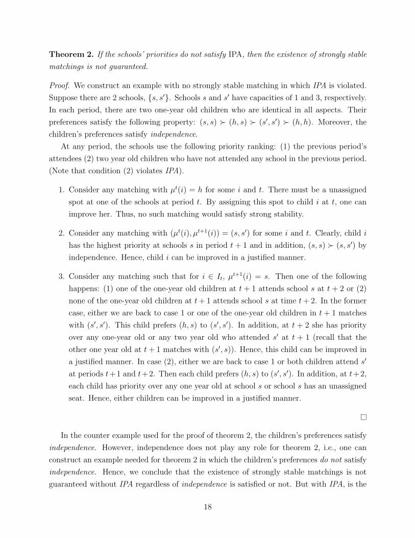
Theorem 2. If the schools’ priorities do not satisfy IPA, then the existence of strongly stable

matchings is not guaranteed.

Proof. We construct an example with no strongly stable matching in which IPA is violated.

Suppose there are 2 schools, {s, s′}. Schools s and s′ have capacities of 1 and 3, respectively.

In each period, there are two one-year old children who are identical in all aspects. Their

preferences satisfy the following property: (s, s) � (h, s) � (s′, s′) � (h, h). Moreover, the

children’s preferences satisfy independence.

At any period, the schools use the following priority ranking: (1) the previous period’s

attendees (2) two year old children who have not attended any school in the previous period.

(Note that condition (2) violates IPA).

1. Consider any matching with µt(i) = h for some i and t. There must be a unassigned

spot at one of the schools at period t. By assigning this spot to child i at t, one can

improve her. Thus, no such matching would satisfy strong stability.

2. Consider any matching with (µt(i), µt+1(i)) = (s, s′) for some i and t. Clearly, child i

has the highest priority at schools s in period t+ 1 and in addition, (s, s) � (s, s′) by

independence. Hence, child i can be improved in a justified manner.

3. Consider any matching such that for i ∈ It, µt+1(i) = s. Then one of the following

happens: (1) one of the one-year old children at t + 1 attends school s at t + 2 or (2)

none of the one-year old children at t+ 1 attends school s at time t+ 2. In the former

case, either we are back to case 1 or one of the one-year old children in t+ 1 matches

with (s′, s′). This child prefers (h, s) to (s′, s′). In addition, at t + 2 she has priority

over any one-year old or any two year old who attended s′ at t + 1 (recall that the

other one year old at t+ 1 matches with (s′, s)). Hence, this child can be improved in

a justified manner. In case (2), either we are back to case 1 or both children attend s′

at periods t+1 and t+2. Then each child prefers (h, s) to (s′, s′). In addition, at t+2,

each child has priority over any one year old at school s or school s has an unassigned

seat. Hence, either children can be improved in a justified manner.

In the counter example used for the proof of theorem 2, the children’s preferences satisfy

independence. However, independence does not play any role for theorem 2, i.e., one can

construct an example needed for theorem 2 in which the children’s preferences do not satisfy

independence. Hence, we conclude that the existence of strongly stable matchings is not

guaranteed without IPA regardless of independence is satisfied or not. But with IPA, is the

18

existence guaranteed? The answer to this question is positive but before we present the

formal result, let us introduce the algorithm used for the existence result.

4.2.1 The Gale-Shapley Deferred Acceptance Algorithm and Its Properties

The Gale and Shapley deferred acceptance algorithm (GS algorithm) was originally designed

to deal with static two-sided matching problems. To run this algorithm at certain period

t, one needs to know the schools’ priority rankings over all school-age children as well as

the children’s preferences over schools. In the class of problems studied in this paper, the

schools’ priority rankings are well defined given the previous period’s matching. However,

the children’s preferences are defined over the pairs of schools since each child can attend

different schools for two consecutive periods. Hence, to run the original GS mechanism, one

needs to derive one period preferences for each child at a given period, based on the past

matchings and the original preferences of the children over the pairs of schools; we do not

want to derive one period preferences based on the future matchings as the current matchings

affect next period’s priority rankings of the schools.

For now, let us assume that at period t, we have derived the one period preference

relation Pi(µt−1) for each i ∈ It−1 ∪ It depending on µt−1 matchings. Let P(µt−1) =

{Pi(µt−1)}i∈It−1∪It . Thus, sPi(µt−1)s′ means that at time t, player i prefers school s to

s′ given the period t− 1 matching µt−1. Note that this definition relies critically on the pre-

vious period’s matching (for example, there could be high switching costs for the children).

With this concept of one-period preferences, we will define stability in a static context that

will be used in some of our proofs.

Definition 9 (Static Stability). Period t matching µt is statically stable under P(µt−1) and

µt−1, if there exists no school-child pair (s, i) such that

1. sPi(µt−1)µt(i),

2. |µt(s)| < rs or/and iBts (µt−1)j for some j ∈ µt(s)

Now we will define the one-period preferences that we will use for the GS algorithm.

Definition 10 (Isolated Preference Relation). For given µt−1,

1. the isolated preference relation for i ∈ It is the preference relation �1i such that s′ �1

i s′′

if and only if (s′, s′) �i (s′′, s′′) for any s′ 6= s′′ ∈ S,

2. the isolated preference relation for i ∈ It−1 is the preference relation �2i (µt−1) de-

pending on previous period’s matching and such that s′ �2i (µt−1)s′′ if and only if

(µt−1(i), s′) �i (µt−1(i), s′′) for any s′ 6= s′′ ∈ S.

19

Here, we remark that for any child whose preferences satisfy independence, the isolated

preferences are independent of the previous period’s matching. Furthermore, the isolated

preferences for one year old child is identical to the ones for the two year old self of the same

child.

The Gale and Shapley deferred acceptance algorithm:

The algorithm is the same in each period, and it only uses the matching of the preceding

period. In period t ≥ 1, assume that the previous period’s matching is obtained by using

the GS algorithm.9 At period t, the schools assign their spots to the all school-age children

in finite rounds as follows:

Round 1: Each child proposes to her first choice according to her isolated preferences.

Each school tentatively assigns its spots to the proposers according to its priority ranking.

If the number of proposers to school s is greater than the number of available spots rs, then

the remaining proposers are rejected.

In general, at:

Round k: Each child who was rejected in the previous round proposes to her next choice

according to her isolated preferences. Each school considers the pool of children who it had

been holding plus the current proposers. Then it tentatively assigns its spots to this pool of

children according to its priority ranking. The remaining proposers are rejected.

The algorithm terminates when no child proposal is rejected and each child is assigned

her final tentative assignment.

Given that the children’s preferences as well as schools’ priority rankings are strict, it is

easy to see that the GS algorithm yields a unique matching. We refer to this matching as

the GS matching and use the notation µGS for it.

With the next result we show that when assuming IPA, strong stability is equivalent to

static stability under isolated preferences.

Lemma 2. If µ is strongly stable then for all t ≥ 0, µt is statically stable under isolated

preferences and µt−1. If for all t ≥ 0, µt is statically stable under isolated preferences and

µt−1, then µ = (µ−1, · · · , µt, · · · ) is

1. weakly stable.

9Recall that period −1 matching is fixed.

20

2. strongly stable if each school’s preferences satisfy IPA.

Proof. See appendix.

Lemma 2 means that to find a strongly stable matching, it suffices to find a stable

matching under isolated preferences in each period, sequentially starting from period 0.

In other words, for the purpose of finding a stable matching, one can treat the daycare

assignment problem as separate school choice problems in different periods. Consequently,

the GS matching is strongly stable as Gale and Shapley (1962) shows that the GS algorithm

yields a stable matching in a static setting. We state the result below.

Theorem 3. The GS matching is weakly stable. Furthermore, if the priority ranking of each

school satisfies IPA, then the GS matching is strongly stable.

As we already mentioned, examples 2 and 3 illustrate the need of strengthening the weak

stability concept into the strong stability one if independence or IPA is not satisfied. However,

theorem 3 demonstrates that IPA is a sufficient condition for the existence of strongly stable

matchings even if independence is not satisfied. In addition, theorem 2 shows that with or

without independence, the existence of strongly stable matchings is not guaranteed without

IPA. In this sense, IPA is a more critical condition than independence for the existence of

strongly stable matchings. Perhaps, this is a good news from the policy maker’s perspective

in the sense that the policy maker can change the schools’ priorities but not the children’s

preferences.

In static settings, one of the most significant results is that the GS matching Pareto

dominates all other stable matchings.10 This result is no longer valid in our daycare assign-

ment problem. In fact, there could be multiple weakly/strongly stable matchings that do

not Pareto dominate one another. The following example illustrates this point.

Example 4. There are 3 schools {s, s1, s2}. All schools have a capacity of one child. There

is no school-age child until period t − 1. At period t − 1, only one child i is 1 year old. At

period t, there are 2 one-year old children {i1, i2}. At period t + 1, child i′ is 1 year old.

If children ı 6= ı′ ∈ {i, i1, i2, i′} have not attended school s = s, s1, s2 in the previous period,

then school s ranks child ı and child ı′ according to the following rankings.

i Bs i1 Bs i2 Bs i′

i Bs1 i′ Bs1 i2 Bs1 i1

i Bs2 i1 Bs2 i2 Bs2 i′

10See Gale and Shapley (1962).

21

Each child’s preferences satisfy independence. Child i’s top choice is (s, s). The prefer-

ences of children i1, i2 and i′ satisfy the following conditions:

(s1, s1) �i1 (s2, s2) �i1 (s, s),

(s, s) �i2 (s2, s2) �i2 (s1, s1),

(s1, s1) �i′ (s2, s2) �i′ (s, s).

The GS matching µGS is as follows: µt−1GS (i) = µtGS(i) = s, µtGS(i1) = µt+1

GS (i1) = s1,

µtGS(i2) = s2, µt+1GS (i2) = s, µt+1

GS (i′) = s2 and µt+2GS (i′) = s1. Thanks to theorem 3, µGS is

weakly stable.

Now let us consider the following matching µ: µt−1(i) = µt(i) = s, µt(i1) = µt+1(i1) = s2,

µt(i2) = s1, µt+1(i2) = s, µt+1(i′) = s1 and µt+2(i′) = s1. It easy to check µ is strongly stable.

Now observe that matching µGS does not Pareto dominate matching µ because child i′

prefers µ to µ. In fact, µ is not Pareto dominated by any strongly stable matching. To see

this, observe that the only matching that Pareto dominates µ is the one in which children

1 and 2 switch their matches in period t. But this is not strongly stable because child i1

justifiably envies child i′ at t+ 1. �

First observe that in example 4 both IPA and independence are satisfied. Hence, the

weakly and strongly stable matchings coincide. Hence, the example above shows that there

may exist mechanisms that produce strongly/weakly stable matchings not Pareto dominated

by the GS matching. This is the first main distinction between the matching produced by

the GS algorithm in the school choice problem versus the daycare assignment problem.

Given the importance of this result when compared to the static case, we state the result

below.

Theorem 4 (The GS matching does not necessarily Pareto dominate all stable matchings).

The GS matching does not necessarily Pareto dominate all weakly/strongly stable matchings.

In the light of example 4, one must explore whether any strongly stable matching Pareto

dominates the GS matching. This, indeed, is impossible which we show in the following

proposition.

Proposition 1 (The GS matching is not Pareto dominated by any strongly stable matching).

If each school’s priority rankings satisfy IPA, then the GS matching is not Pareto dominated

by any other strongly stable matchings.

Sketch of the Proof. Here, we will only sketch the proof. The formal proof is in the appendix.

The proof is by contradiction: suppose that there exists a strongly stable matching µ

that Pareto dominates the GS matching, µGS. We proceed in 3 steps.

22

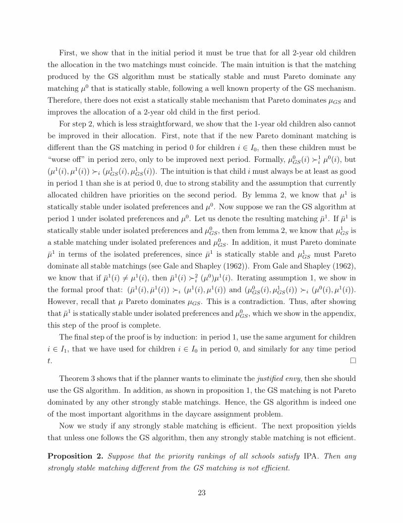
First, we show that in the initial period it must be true that for all 2-year old children

the allocation in the two matchings must coincide. The main intuition is that the matching

produced by the GS algorithm must be statically stable and must Pareto dominate any

matching µ0 that is statically stable, following a well known property of the GS mechanism.

Therefore, there does not exist a statically stable mechanism that Pareto dominates µGS and

improves the allocation of a 2-year old child in the first period.

For step 2, which is less straightforward, we show that the 1-year old children also cannot

be improved in their allocation. First, note that if the new Pareto dominant matching is

different than the GS matching in period 0 for children i ∈ I0, then these children must be

“worse off” in period zero, only to be improved next period. Formally, µ0GS(i) �1

i µ0(i), but

(µ1(i), µ1(i)) �i (µ1GS(i), µ1

GS(i)). The intuition is that child i must always be at least as good

in period 1 than she is at period 0, due to strong stability and the assumption that currently

allocated children have priorities on the second period. By lemma 2, we know that µ1 is

statically stable under isolated preferences and µ0. Now suppose we ran the GS algorithm at

period 1 under isolated preferences and µ0. Let us denote the resulting matching µ1. If µ1 is

statically stable under isolated preferences and µ0GS, then from lemma 2, we know that µ1

GS is

a stable matching under isolated preferences and µ0GS. In addition, it must Pareto dominate

µ1 in terms of the isolated preferences, since µ1 is statically stable and µ1GS must Pareto

dominate all stable matchings (see Gale and Shapley (1962)). From Gale and Shapley (1962),

we know that if µ1(i) 6= µ1(i), then µ1(i) �2i (µ0)µ1(i). Iterating assumption 1, we show in

the formal proof that: (µ1(i), µ1(i)) �i (µ1(i), µ1(i)) and (µ0GS(i), µ1

GS(i)) �i (µ0(i), µ1(i)).

However, recall that µ Pareto dominates µGS. This is a contradiction. Thus, after showing

that µ1 is statically stable under isolated preferences and µ0GS, which we show in the appendix,

this step of the proof is complete.

The final step of the proof is by induction: in period 1, use the same argument for children

i ∈ I1, that we have used for children i ∈ I0 in period 0, and similarly for any time period

t.

Theorem 3 shows that if the planner wants to eliminate the justified envy, then she should

use the GS algorithm. In addition, as shown in proposition 1, the GS matching is not Pareto

dominated by any other strongly stable matchings. Hence, the GS algorithm is indeed one

of the most important algorithms in the daycare assignment problem.

Now we study if any strongly stable matching is efficient. The next proposition yields

that unless one follows the GS algorithm, then any strongly stable matching is not efficient.

Proposition 2. Suppose that the priority rankings of all schools satisfy IPA. Then any

strongly stable matching different from the GS matching is not efficient.

23

Proof. Consider any strongly stable matching µ with some period t matching that is different

from the one that the GS algorithm under isolated preferences and µt−1 yields. Consider

any i ∈ It. Then µt(i) = µt+1(i) or (µt+1(i), µt+1(i)) �i (µt(i), µt(i)); otherwise, µ is not

strongly stable because, in this case, child i would have the higher priority at school µt(i)

and (µt(i), µt(i)) �i (µt(i), µt+1(i)) by assumption 1.

For each child i ∈ It−1 ∪ It, define her preference relation to be P ti such that sP ti s′ if and

only if

(µt−1(i), s) �i (µt−1(i), s′) whenever i ∈ It−1

(s, µt+1(i)) �i (s′, µt+1(i)) whenever i ∈ It

Because µ is strongly stable, there cannot exist any school-child pair (s, i) such that

1. (µt−1(i), s) �i (µt−1(i), µt(i)) or (s, µt+1(i)) �i (µt(i), µt+1(i)),

2. |µt(s)| < rs or/and iBts (µt−1)j for some j ∈ µt(s).

In terms of P , these conditions mean that there is no school-child pair (s, i) such that

1. sP tiµt(i),

2. |µt(s)| < rs or/and iBts (µt−1)j for some j ∈ µt(s).

In other words, µt is a statically stable matching under P and µt−1.

Consider matching µ such that µτ = µτ for all τ 6= t but µt is the resulting matching

from the GS algorithm under P and µt−1.

From Gale and Shapley (1962), we know that µt must Pareto dominate every other stable

matching under P and µt−1. This and that µt is a statically stable matching under P and

µt−1 imply that µt(i)Piµt(i) for all i ∈ It−1∪It if µt(i) 6= µt(i). Consequently, if µt(i) 6= µt(i)

for some i ∈ It−1, then (µt−1(i), µt(i)) �i (µt−1(i), µt(i)). Similarly, if µt(i) 6= µt(i) for some

i ∈ It then (µt(i), µt+1(i)) �i (µt(i), µt+1(i)). Now consider µ and µ. Clearly, µ Pareto

dominates µ if µt(i) 6= µt(i) for some i ∈ It−1 ∪ It. Hence, it must be that µt(i) = µt(i) for

all i ∈ It−1 ∪ It.Consider µ such that µτ = µτ for all τ 6= t but µt is the resulting matching from the

GS algorithm under isolated preferences and µt−1. Clearly, µt−1 = µt−1, hence, the priority

rankings of the schools are the same under both µ and µ. In addition, for each j ∈ It−1, the

isolated preference relation�2j (µt−1) is equivalent to Pj. Now consider any child j ∈ It. Then

under P , the relative ranking of µt+1(j) weakly improves from the one under �1j . In all other

aspects, Pj and�1j are the same. Now recall that µt(i) = µt(i) for all i ∈ It−1∪It. In addition,

recall that µt(i) = µt+1(i) or (µt+1(i), µt+1(i)) �i (µt(i), µt(i)). Therefore, under both Pj

24

and �1j , the set of schools that are strictly preferred to µt(j) is the same. Consequently, we

obtain that under P and isolated preferences, for each j ∈ I t−1 ∪ I t, the set of schools that

are strictly preferred to µt(j) is the same. In addition, because the GS algorithm is used for

both cases and µt(j) = µt(j) for all j ∈ It−1 ∪ It, it must be µt = µt thanks to theorem 9 in

Dubins and Freedman (1981). Consequently, µt = µt, which contradicts that µt differs from

the matching that the GS algorithm yields.

Proposition 2 means that if any strongly stable matching is efficient, then it must be the

GS matching. However, from Roth (1982), it is well known that the GS matching (in static

settings) is not necessarily Pareto efficient. This is still the case in our setting because the

school choice problem is a special case of our problem as we pointed out in Remark 1.

Henceforth, we will always assume that the children’s preferences satisfy Independence

and the schools’ priorities satisfy IPA because these assumptions do not play any role in

the results we will present next. In other words, we are concentrating on the cases with a

minimal history dependence.

5 Strategy Proofness and Stability: Impossibility Re-

sult

It is well known that in static settings, when the GS mechanism is applied, reporting one’s

true preferences is a weakly dominant strategy. Hence, the mechanism is strategy-proof. In

this section, we explore if any mechanism is strategy-proof and strongly stable.

Even when independence and IPA are satisfied, strategy-proofness is more difficult to

achieve in the daycare assignment problem. In static problems, a child has a motive to

misreport her preferences only if she can obtain a better placement. This motive is also

present in the daycare assignment problem. To be specific, a child will misreport her pref-

erences if she can obtain a better placement in a period without hurting her placement in

the other period. But we know from the school choice literature that there are important

strategy-proof mechanisms such as the GS or Top Trading Cycles (TTC) algorithm. How-

ever, in the daycare assignment problem, there is another motive which is not present in the

school choice problem: a child misrepresents her preferences to affect the priority rankings

of schools when she is two. This way she obtains a better placement when she is two, but

she sacrifices her placement when she is one. The second motive is indeed very strong that

derives the following impossibility result.

Theorem 5 (Impossibility Result). The existence of a strategy-proof and weakly stable mech-

anism is not guaranteed.

25

Proof. Consider the following example: there are 4 schools {s, s, s1, s2}. All schools have a

capacity of one child. There is no school-age child until period t− 1. Suppose It−1 = {i, ı},It = {i1, i2}, It+1 = {i′} and Iτ = ∅ for all τ ≥ t + 2. In addition, school s′ = s, s, s1, s2

prioritizes the children as follows under the assumption that no child attended s′ in the

previous period:

i Bs i′ Bs i1 Bs i2

i Bs1 i1 Bs1 i2 Bs1 i′

i Bs2 i1 Bs2 i′ Bs2 i2

ı Bs i1 Bs i′ Bs i2

We consider two preference profiles which differ from each other in child i1’s preferences.

Child i’s top choice is (s, s) while child ı’s is (s, s). The preferences of children i2 and i′

satisfy the following conditions:

(s2, s2) �i2 (s1, s1) �i2 (s, s) �i2 (s, s)

(s2, s2) �i′ (s, s) �i′ (s1, s1) �i2 (s, s)

Child i1’s preference ordering is �1i1

under preference profile 1 and is �2i1

under profile 2.

These preferences are given as follows:

(s, s) �1i1

(s1, s1) �1i1

(s2, s2) �1i1

(s, s)

(s, s) �2i1

(s, s) �1i1

(s2, s2) �2i1

(s1, s1)

In addition, suppose (s2, s) �1i1

(s1, s1).

Now we prove that there is no strategy-proof and weakly stable mechanism in the above

example. We proceed in 3 steps.

Step 1. Under profile 1, the only weakly stable matching µ is as follows: µt−1(i) = µt(i) = s,

µt−1(ı) = µt(ı) = s, µt(i1) = µt+1(i1) = s1, µt(i2) = µt+1(i2) = s2, µt+1(i′) = s and

µt+2(i′) = s2.

Proof of Step 1. It is easy to see that µ is the GS matching, hence, is weakly stable. Now

the only thing we need to show is that no other matching is weakly stable under profile 1.

Let µ be weakly stable. It is clear that µt−1(i) = µt(i) = s, µt−1(ı) = µt(ı) = s and

µt+2(i′) = s2. Consequently, we obtain that µt(i1) = s1 because child i1 has higher priority

in school s1 at period t than anyone but i. However, i must match with s at period t. Hence,

µt(i1) = s1. This implies that µt(i2) = s2. Then i2 has the highest priority at school s2 at

period t+1. Since s2 is the top choice for i2, µt+1(i2) = s2. Consequently, µt+1(i′) = s which

means µt+1(i1) = s1. Now we have shown that µ = µ.

Step 2. Under profile 2, the only weakly stable matching µ is as follows: µt−1(i) = µt(i) = s,

26

µt−1(ı) = µt(ı) = s, µt(i1) = s2, µt(i2) = s1, µt+1(i1) = s, µt+1(i2) = s1, µt+1(i′) = s2 and

µt+2(i′) = s2.

Proof of Step 2. It is easy to see that µ is the GS matching under profile 2, hence is weakly

stable. Now we only need to show that no other matching is weakly stable under profile 2.

Let µ be a weakly stable matching. It is clear that µt−1(i) = µt(i) = s, µt−1(ı) = µt(ı) = s

and µt+2(i′) = s2. Consequently, we obtain that µt(i1) = s2 because child i1 has higher

priority in school s2 at period t than i2. This means that µt(i2) = s1.

Now let us argue that µt+1(i′) = s2. If not, µt+1(i1) = s2; otherwise, child i′ has higher

priority than child i2 at school s2 and s2 is the top choice of child i′. Hence, this contradicts

with µ being weakly stable. Thus, µt+1(i1) = s2. But because (s2, s) �2i1

(s2, s2) and child i1

has higher priority at school s than anyone but ı, µ is weakly stable. This is a contradiction.

Hence, µt+1(i′) = s2.

Because µt+1(i′) = s2, µt+1(i1) = s as i1 has higher priority at school s than i2. Conse-

quently, µt+1(i2) = s1. This means µ = µ

Step 3. For this example, no strategy-proof and weakly stable mechanism exists.

Proof of Step 3. Consider any weakly stable mechanism. This mechanism must yield match-

ing µ under profile 1 and matching µ under profile 2. Under profile 1, by truthfully reporting

her preferences, child i1 is placed at school s1 at periods t and t+ 1. However, by misreport-

ing her preference as if under profile 2, she is placed at school s2 in period t and at school

s in period t + 1. By assumption, (s2, s) �1i1

(s1, s1). Consequently, child i1 misreports her

preferences under profile 1, hence, any weakly stable mechanism is not strategy-proof.

In the example used for the proof of theorem 5, type 1 child i1 likes school s better than

any other school. Clearly, there is no chance that she can attend s in period t. In addition,

she cannot attend s at t + 1 because child i′ attends s. But observe that child i′ wants to

attend school s2 but cannot do so because child i2 attends s2. The most important aspect

is that child i2 has higher priority over child i′ at school s2 in period t+ 1 only because she

attends school s2 in period t. Child i1 can eliminate child i2’s advantage over i′ if she attends

school s2 in period t. By doing this, i1 enables i′ to attend s2 at t+ 1. Ultimately, she frees

a spot at school s for herself at t+ 1. This is the reason why type 1 child i1 has an incentive

to misreport her preferences.

Remark 4. For theorem 5, both the OLG structure of the daycare assignment problem

and the history dependence of the schools’ priorities play indispensable roles. In remark

2, we already mentioned that without OLG structure, all the existing results in the school

choice problem will be valid. Now let us discuss why the history dependence of the schools’

priorities is critical for theorem 5 even with the OLG structure. To see this, suppose that the

27

children’s preferences satisfy independence and somehow the schools’ priorities at any period

are independent of the previous period’s matching–in particular, a child could be misplaced

from the daycare she is currently allocated to. In this case, the GS algorithm using the

isolated preferences of the children must be strategy-proof. Let us discuss why this is the

case. For the GS algorithm, one has to report her preferences over the pairs of schools. But

this, in fact, is equivalent to the case in which the school-age children report their isolated

preferences in each period and the algorithm is run sequentially because the GS algorithm uses

the isolated preference. As the preferences satisfy independence and the schools’ preferences

are independent of history, any child’s reported isolated preferences in one period do not

affect her placement in the other period. Now recall that the GS algorithm is strategy-proof

in the static settings. Hence, by misreporting one’s isolated preferences in some period, she

is worse off in that period without affecting her placement in the other period. Accordingly,

no one misreports her isolated preferences. Thus, the GS mechanism is strategy-proof.

Remark 5. In the previous remark, we argued that the history dependence of the schools’

priorities is crucial for theorem 5. Then in the example used in the proof of theorem 5, child

i2 is forced out of school s2 at period t+1. This is a case one should avoid. Therefore, under

the restriction that no 2-year old child can be forced out of the school she attended in the

previous period, theorem 5 is valid even when the schools’ priorities are independent of the

previous period’s matching.

Theorem 5 has two important, direct consequences which we present next.

Corollary 1. 1. The existence of a strongly stable and strategy-proof mechanism is not

guaranteed.

2. The GS mechanism using the children’s isolated preferences is not necessarily strategy-

proof.

Proof. Recall that each strongly stable matching is weakly stable. This and theorem 5 prove

item 1 of the corollary.

6 Efficiency and Strategy Proofness

We have shown that the well known GS algorithm, which is widely used in the school choice

problem, is not a particularly appealing algorithm for the daycare assignment problem, since

it is not necessarily strategy-proof.

Most importantly, we showed that stability and strategy-proofness maybe incompatible

for the daycare assignment problem. This suggests that eliminating justified envy may not

28

be the most appropriate objective when designing an assignment mechanism, at least not if

strategy-proofness is desired. In the remaining sections of this paper, we investigate whether

strategy-proofness is compatible with efficiency. However, before doing so, let us consider

some properties of efficient matchings.

From the school choice literature, we know that the Top Trading Cycles (TTC) or the

Serial Dictatorship mechanisms yield stable matchings. Hence, one might expect that these

algorithms using the isolated preferences of the children yield efficient matchings. In other

words, one may expect that a result analogous to the result of lemma 2 will hold for efficiency

as well. We will demonstrate that this is not necessarily the case. But first, let us define the

Autarkic efficiency concept.

Definition 11 (Autarkic Efficiency). Matching µ satisfies Autarkic Efficiency if for any

t ≥ 0, there does not exist period t matching µt such that (µ−1, · · · , µt−1, µt, µt+1, · · · ) Pareto

dominates µ.

For Autarkic efficiency, one considers only one period deviations. Hence, it is clear that

all efficient matchings satisfy Autarkic efficiency. Now the following examples show that

Autarkic efficiency is not equivalent to efficiency.

Example 5. Suppose in period 0, two children i1 and i2 are two years old and two children

j1 and j2 are one year old. There are 4 schools s1, s2, s3 and s4 and each school has a capacity

of 1 child. The schools’ priorities are given as follows under the assumption that the children

have not attended any school in the previous period:

i1 Bs1 i2 Bs1 j1 Bs1 j2

i2 Bs2 i1 Bs2 j2 Bs2 j1

i1 Bs3 i2 Bs3 j1 Bs3 j2

i1 Bs4 i2 Bs4 j2 Bs4 j1

Child i1’s top choice is s1 while child i2’s is s2. The other two children’s preferences satisfy

the following conditions:

(s2, s2) �j1 (s1, s1) �j1 (s4, s2) �j1 (s3, s1) �j1 (s3, s3) �j1 (s4, s4)

(s2, s2) �j2 (s1, s1) �j2 (s3, s1) �j2 (s4, s2) �j2 (s3, s3) �j2 (s4, s4)

Now consider the following matching µ: µ0(i1) = s1, µ0(i2) = s2, µ0(j1) = s3, µ0(j2) = s4,

µ1(j1) = s1, µ1(j2) = s2. Matching µ satisfies Autarkic efficiency. However, µ is not

Pareto efficient as it is dominated by the matching µ: µ0(i1) = s1, µ0(i2) = s2, µ0(j1) = s4,

µ0(j2) = s3, µ1(j1) = s2, µ1(j2) = s1.

29

Loosely speaking, in example 5, children j1 and j2 are assigned “extreme” allocations

under matching µ. Hence, these children j1 and j2 can hedge against the extreme allocations

by “trading” their allocations. This is one reason why Autarkic efficiency is not equivalent

to efficiency. One should observe that in this case trade happens between the children from

the same generation. Hence, the infiniteness of time does not play any significant role in

example 5. However, one can construct an example in which a matching satisfying Autarkic

efficiency fails to be efficient because of the intergenerational trades. We demonstrate this

point in the following example.

Example 6. In each period, there are two 1-year old children in each period {it, jt} and

there are four schools {s1, s2, s3, s4}. For this example, we will only specify the schools’ top

ranked school-age child under the assumption that all children stayed home in the previous

period. School s1 and s2 give their respective highest priorities to children i and j who are 1

in odd periods. On the other hand, school s3 and s4 give their respective highest priorities to

children i and j who are 1 in even periods. The children’s preferences are as follows.

• Child i−1’s top choice is s1 while for child j−1, s3 �1j−1 s2 �1

j−1 s4.

• For child i0, s1 �1i0 s3 �1

i0 s2 while child j0’s top choice is s4.

• For child i1, s4 �1i1 s1 �1

i1 s3 while child j1’s top choice is s2.

• Child i2’s top choice is s3 while for child j2, s2 �1j2 s4 �1

j2 s1.

• For t ≥ 3, child it (jt) has the same preferences as child it−4 (jt−4).

In addition, each child prefers being placed at the school of her third choice when she is 1

and at her most preferred school when she is two to being placed at the school of her second

choice for 2 periods.

Consider the following matching µ: in any period, school s1 matches with the school-age

child i who is 1 in an odd period, s2 with j who is 1 in an odd period, s3 with i who is 1 in

an even period, and school s4 with j who is 1 in an even period. Observe that in each period

exactly 1 younger and 1 older children match with their second choice school. The others

match with their top choice. It is easy to see that µ satisfies Autarkic efficiency. Now let us

alter µ in the following way: in each period, the two children who are placed at her second

choice school trades their schools. This way the older of the two children is placed at her

first choice school while the younger one is placed at her third choice school. One can easily

see that the new altered matching Pareto dominates µ.

30

Observe that in the above example, the infiniteness of time plays an important role. To

see this, let us check why µ is not efficient. Matching µ places one younger and one older

children at their second choice schools in each period. Each of these child prefers being

placed in her third choice school when she is one and at her most preferred school in the

following period to being placed at her second choice school in both periods. Hence, the

younger child would agree to give her spot away and obtain a spot at a worse school as long

as she obtains a spot at her most preferred school in the following period. Accordingly, µ is

not efficient because one younger child can trade her spot with an older child in each period.

If time stops at some point, then the younger child at that time would not agree to this

trade. This is why the infiniteness of time is crucial in example 6. This phenomenon is also

observed in the standard overlapping generations models.

Examples 5 and 6 have an important implication: not all mechanisms that deliver match-

ings satisfying Autarkic efficiency are necessarily efficient even if the children’s preferences

satisfy independence. For example, the TTC mechanism using isolated preferences does not

necessarily yield an efficient matching. As we will discuss whether the TTC mechanism is

strategy-proof, let us consider the TTC mechanism in the next subsection.

6.1 The Top Trading Cycles Mechanism

The TTC mechanism was introduced in Abdulkadiroglu and Sonmez (2003).11 Next we will

state the formal definition of the TTC mechanism.

In each period, we assume that the preceding period’s matching is produced by the TTC

mechanism according to the isolated preferences of children. In period t:

Round 1 : Each child points to her preferred school. Each school points to its highest

ranked child. The process goes on, until it reaches a cycle, which it eventually will. A

cycle can be written as {i1, s1, i2, s2, · · · , ik, sk}, where here, sj is child i′js preferred school,

whereas child il is the highest ranked child in school sl−1, for l = 2, ..., k; and child i1 is the

highest ranked child at school sk. All children in the cycle are allocated to their preferred

school.

In general, at:

Round k : All children allocated in rounds 1,...,k − 1 do not participate in step k. Each

remaining child points to its preferred school, among the set of schools with remaining spots.

Each pointed school points to the highest priority child among the remaining children. The

11The TTC mechanism is inspired by Shapley and Scarf (1974) and Roth and Postlewaite (1977).

31

process goes on until it reaches a cycle, which it eventually will. All children in the cycle are

allocated to the schools that they have pointed to.

The process continues until all children are allocated.

As we already hinted, the top trading cycle mechanism is not necessarily efficient. Given

the importance of the TTC mechanism in the school choice problem, let us state this result

in the following proposition.

Proposition 3 (TTC is not necessarily Pareto Efficient). If the TTC mechanism is applied

at every period using the isolated preferences of the children, then the resulting matching is

not necessarily Pareto efficient.

Proof. Consider example 5 and observe that µ is the matching from the TTC mechanism.

As we mentioned µ is not efficient.

Note that in example 5, not only the TTC mechanism is not necessarily efficient, but

also a variation of it, done by cohorts. Precisely, consider the following mechanism. At any

period t, the children born in period t−1 are allocated according to the TTC mechanism (see

Abdulkadiroglu and Sonmez (2003)). Once every children i ∈ It−1 is allocated, most schools

will have less, if any, spots available. Consider only the schools with open spots and use the

TTC mechanism for the generation born in period t, where from the initial number of spots

for each school, we have subtracted the number of 2-year-old children already allocated. For

this round, consider only the priority of schools over the children of generation t. i.e., a

young child cannot replace an already allocated 2-year-old child. This variation of the TTC

mechanism is also is not Pareto efficient.

In the example below, we show that the TTC mechanism (using isolated preferences)

may not be strategy-proof.

Example 7 (TTC may not be Strategy-Proof). Assume that there are 4 schools {s, s1, s2, s3},and 4 children: {i, i1, i2, i3}, with i ∈ I−1 and {i1, i2, i3} ∈ I0. Assume also that It = ∅ for all

t ≥ 1. School s = s, s1, s2, s3 prioritizes the children as follows assuming that these children

has not attended s in the previous period:

i Bs i2 Bs i1

i1 Bs1 j, ∀j 6= i1

i2 Bs2 j, ∀j 6= i2

i1 Bs3 i3 Bs3 j, ∀j 6= i1, i3

32

The children’s preferences are:

s �i s1 �i s2 �i s3

s �i1 s1 �i1 s2 �i1 s3

s3 �i2 s �i2 s2 �i2 s1

s3 �i3 s1 �i3 s2 �i3 s

In addition, child i1 prefers (s′, s) to (s1, s1). The matching resulting from the TTC is:

µ0 (i) = s, µ0 (i1) = s1, µ0(i2) = s2, µ0 (i3) = s3, µ1 (i1) = s1, µ1 (i2) = s and µ1 (i3) = s3.

Suppose that i1 misreports its preferences to be: s �i1 s2 �i1 s1 �i1 s3, while all others

report truthfully. The resulting matching is given as follows: µ0 (i) = s, µ0 (i1) = s2 ,

µ0 (i2) = s3, µ0 (i3) = s1, µ1 (i1) = s, µ1 (i2) = s3 and µ1 (i3) = s1.

Note that under truth-telling, i1’s allocation was: (s1, s1), while after misreporting it is

(s2, s). Thus, i1 has improved herself overall by taking s2 in the first period and altering the

priority of s3 for the following period. �

Observe that the example above shows that a variation of the TTC which is done by

cohorts is not strategy-proof.

6.2 Strategy-Proofness and Efficiency

The previous subsection leads to the question of whether strategy-proofness and efficiency

are compatible. The answer is positive and to show this, we use a version of the serial dictator

algorithm adapted to our setting. We will argue that this algorithm is strategy-proof and

efficient. Before formalizing the algorithm, recall that at period t, nt number of children are

one and they are indexed 1 through nt. The algorithm runs as follows:

At period k:

All 2-year old children choose the school that they want to attend in an increasing order

according to their indices. All children obtain their top spot as long as the chosen school

has available seats. When a school has filled its slots, the child moves on to her next best

choice.

When all 2-year old children have been allocated, then all 1-year old children choose their

preferred school with open slots following an increasing order according to their indices.

Given that at any given period there is a finite number of school-age children, this is a

well-defined mechanism. Moreover, it is easy to verify that the proposed algorithm is both

33

strategy-proof and efficient.12

7 Conclusion

In this paper we have introduced the daycare assignment problem. This problem differs from

the school choice problem due to its OLG structure. We have proved some negative results

concerning well-known mechanisms, even when preferences satisfy consistency across periods,

and schools’ priorities are linked only in a very weak sense (priorities are history dependent

only through currently allocated children, and are otherwise the same). In particular, we

have shown that the GS and the TTC mechanisms, both commonly used in the school

choice problem, are not necessarily strategy-proof in the daycare assignment problem. We

have extended these insights to show that in some cases, no strongly stable and strategy

proof mechanism exists.

We concluded by presenting a version of the serial dictator, adapted to our setting, and

arguing that it is strategy-proof and efficient.

Appendix A: Aarhus Assignment Mechanism13

ASSIGNMENT RULES In brief, spots are assigned in this order:

1. Children with special needs, e.g. children with disabilities

2. Children with siblings in the same daycare

3. Immigrant children who after expert valuations are considered in need of special assis-

tance in daycare

4. The oldest child who is listed for a guaranteed place in his or her own district (i.e. not

at a particular daycare) .

5. The oldest child who is listed for a guarantee place in the local warranty district.

Aarhus Municipality is divided into 8 major warranty districts. A warranty district

consists of one to several districts.

6. The oldest child listed for a guarantee place from a different warranty district.

12One can use the random serial dictatorship algorithm which is a slight variation of the serial dictatorshipalgorithm. The random serial dictatorship algorithm is strategy-proof and ex-post efficient but not necessarilyex-ante efficient.

13For the original document see: https://www.borger.dk/selvbetjening/sider/fakta.aspx?sbid=8632

34

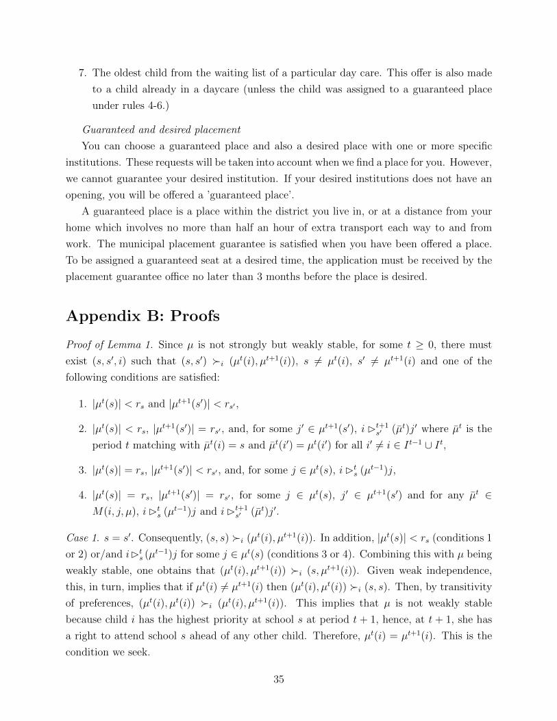
7. The oldest child from the waiting list of a particular day care. This offer is also made

to a child already in a daycare (unless the child was assigned to a guaranteed place

under rules 4-6.)

Guaranteed and desired placement

You can choose a guaranteed place and also a desired place with one or more specific

institutions. These requests will be taken into account when we find a place for you. However,

we cannot guarantee your desired institution. If your desired institutions does not have an

opening, you will be offered a ’guaranteed place’.

A guaranteed place is a place within the district you live in, or at a distance from your

home which involves no more than half an hour of extra transport each way to and from

work. The municipal placement guarantee is satisfied when you have been offered a place.

To be assigned a guaranteed seat at a desired time, the application must be received by the

placement guarantee office no later than 3 months before the place is desired.

Appendix B: Proofs

Proof of Lemma 1. Since µ is not strongly but weakly stable, for some t ≥ 0, there must

exist (s, s′, i) such that (s, s′) �i (µt(i), µt+1(i)), s 6= µt(i), s′ 6= µt+1(i) and one of the

following conditions are satisfied:

1. |µt(s)| < rs and |µt+1(s′)| < rs′ ,

2. |µt(s)| < rs, |µt+1(s′)| = rs′ , and, for some j′ ∈ µt+1(s′), i Bt+1s′ (µt)j′ where µt is the

period t matching with µt(i) = s and µt(i′) = µt(i′) for all i′ 6= i ∈ I t−1 ∪ I t,

3. |µt(s)| = rs, |µt+1(s′)| < rs′ , and, for some j ∈ µt(s), iBts (µt−1)j,

4. |µt(s)| = rs, |µt+1(s′)| = rs′ , for some j ∈ µt(s), j′ ∈ µt+1(s′) and for any µt ∈M(i, j, µ), iBt

s (µt−1)j and iBt+1s′ (µt)j′.

Case 1. s = s′. Consequently, (s, s) �i (µt(i), µt+1(i)). In addition, |µt(s)| < rs (conditions 1

or 2) or/and iBts (µt−1)j for some j ∈ µt(s) (conditions 3 or 4). Combining this with µ being

weakly stable, one obtains that (µt(i), µt+1(i)) �i (s, µt+1(i)). Given weak independence,

this, in turn, implies that if µt(i) 6= µt+1(i) then (µt(i), µt(i)) �i (s, s). Then, by transitivity

of preferences, (µt(i), µt(i)) �i (µt(i), µt+1(i)). This implies that µ is not weakly stable

because child i has the highest priority at school s at period t + 1, hence, at t + 1, she has

a right to attend school s ahead of any other child. Therefore, µt(i) = µt+1(i). This is the

condition we seek.

35

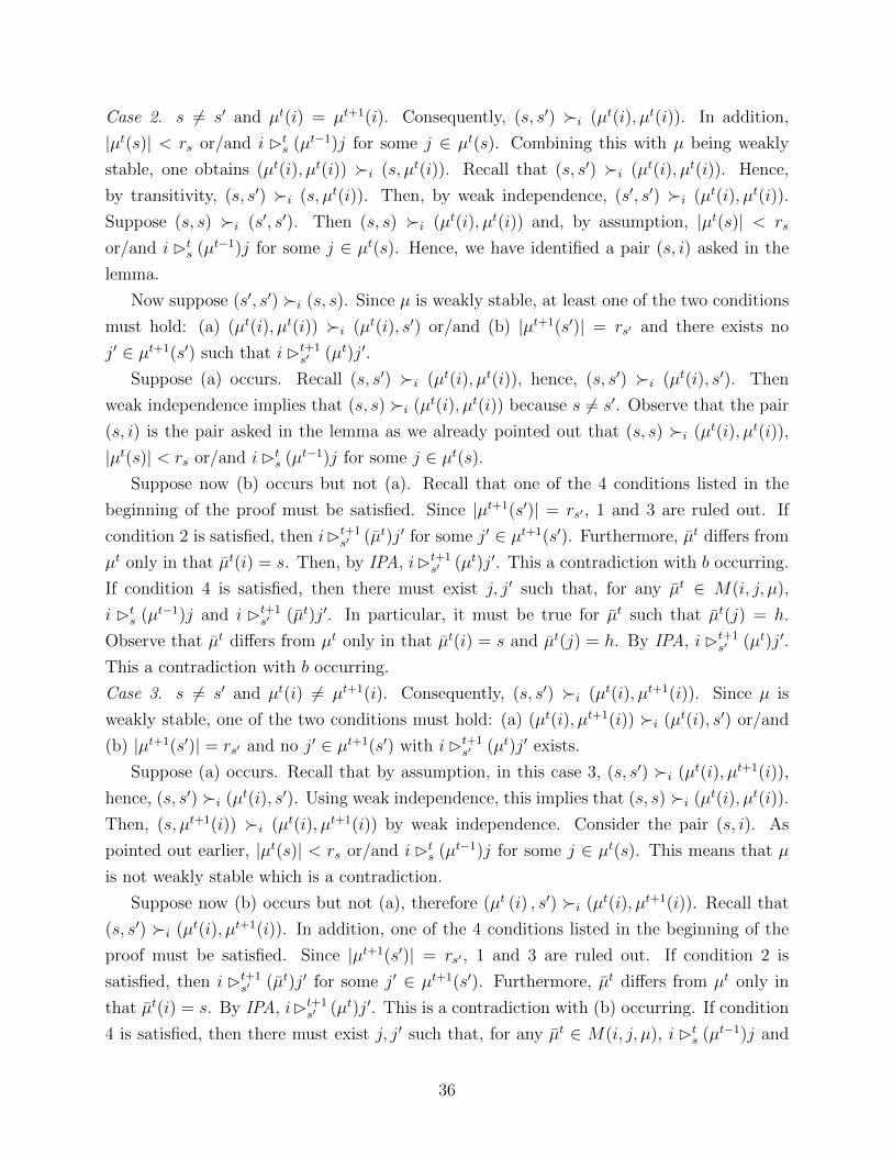
Case 2. s 6= s′ and µt(i) = µt+1(i). Consequently, (s, s′) �i (µt(i), µt(i)). In addition,

|µt(s)| < rs or/and i Bts (µt−1)j for some j ∈ µt(s). Combining this with µ being weakly

stable, one obtains (µt(i), µt(i)) �i (s, µt(i)). Recall that (s, s′) �i (µt(i), µt(i)). Hence,

by transitivity, (s, s′) �i (s, µt(i)). Then, by weak independence, (s′, s′) �i (µt(i), µt(i)).

Suppose (s, s) �i (s′, s′). Then (s, s) �i (µt(i), µt(i)) and, by assumption, |µt(s)| < rs

or/and i Bts (µt−1)j for some j ∈ µt(s). Hence, we have identified a pair (s, i) asked in the

lemma.

Now suppose (s′, s′) �i (s, s). Since µ is weakly stable, at least one of the two conditions

must hold: (a) (µt(i), µt(i)) �i (µt(i), s′) or/and (b) |µt+1(s′)| = rs′ and there exists no

j′ ∈ µt+1(s′) such that iBt+1s′ (µt)j′.

Suppose (a) occurs. Recall (s, s′) �i (µt(i), µt(i)), hence, (s, s′) �i (µt(i), s′). Then

weak independence implies that (s, s) �i (µt(i), µt(i)) because s 6= s′. Observe that the pair

(s, i) is the pair asked in the lemma as we already pointed out that (s, s) �i (µt(i), µt(i)),

|µt(s)| < rs or/and iBts (µt−1)j for some j ∈ µt(s).

Suppose now (b) occurs but not (a). Recall that one of the 4 conditions listed in the

beginning of the proof must be satisfied. Since |µt+1(s′)| = rs′ , 1 and 3 are ruled out. If

condition 2 is satisfied, then iBt+1s′ (µt)j′ for some j′ ∈ µt+1(s′). Furthermore, µt differs from

µt only in that µt(i) = s. Then, by IPA, iBt+1s′ (µt)j′. This a contradiction with b occurring.

If condition 4 is satisfied, then there must exist j, j′ such that, for any µt ∈ M(i, j, µ),

i Bts (µt−1)j and i Bt+1

s′ (µt)j′. In particular, it must be true for µt such that µt(j) = h.

Observe that µt differs from µt only in that µt(i) = s and µt(j) = h. By IPA, iBt+1s′ (µt)j′.

This a contradiction with b occurring.

Case 3. s 6= s′ and µt(i) 6= µt+1(i). Consequently, (s, s′) �i (µt(i), µt+1(i)). Since µ is

weakly stable, one of the two conditions must hold: (a) (µt(i), µt+1(i)) �i (µt(i), s′) or/and

(b) |µt+1(s′)| = rs′ and no j′ ∈ µt+1(s′) with iBt+1s′ (µt)j′ exists.

Suppose (a) occurs. Recall that by assumption, in this case 3, (s, s′) �i (µt(i), µt+1(i)),

hence, (s, s′) �i (µt(i), s′). Using weak independence, this implies that (s, s) �i (µt(i), µt(i)).

Then, (s, µt+1(i)) �i (µt(i), µt+1(i)) by weak independence. Consider the pair (s, i). As

pointed out earlier, |µt(s)| < rs or/and i Bts (µt−1)j for some j ∈ µt(s). This means that µ

is not weakly stable which is a contradiction.

Suppose now (b) occurs but not (a), therefore (µt (i) , s′) �i (µt(i), µt+1(i)). Recall that

(s, s′) �i (µt(i), µt+1(i)). In addition, one of the 4 conditions listed in the beginning of the

proof must be satisfied. Since |µt+1(s′)| = rs′ , 1 and 3 are ruled out. If condition 2 is

satisfied, then i Bt+1s′ (µt)j′ for some j′ ∈ µt+1(s′). Furthermore, µt differs from µt only in

that µt(i) = s. By IPA, iBt+1s′ (µt)j′. This is a contradiction with (b) occurring. If condition

4 is satisfied, then there must exist j, j′ such that, for any µt ∈ M(i, j, µ), i Bts (µt−1)j and

36

iBt+1s′ (µt)j′. Fix µt such that µt(j) = h. Observe that µt differs from µt only in that µt(i) = s

and µt(j) = h. By IPA, iBt+1s′ (µt)j′. This is a contradiction with (b) occurring.

Proof of Lemma 2. Necessity. Assume µ is strongly stable. We need to show that for all t,

µt is statically stable under isolated preferences and µt−1. Suppose otherwise. Then there

must exist, t, and a school-child pair (s, i) such that

1. if i ∈ It, then s �1i µ

t(i) and at least one of the following is satisfied: |µt(s)| < rs

or/and iBts (µt−1)j for some j ∈ µt(s),

2. if i ∈ It−1, then s �2i (µt−1)µt(i) and at least one of the following is satisfied: |µt(s)| <

rs or/and iBts (µt−1)j for some j ∈ µt(s).

Suppose i ∈ It. Then we are in case 1. Since µ is weakly stable, the following 2 conditions

cannot be satisfied at the same time: (a) (s, µt+1(i)) �i (µt(i), µt+1(i)) and (b) |µt(s)| < rs

and/or i Bts (µt−1)j for some j ∈ µt(s). If (b) is not true, then this is a contradiction

because (s, i) must satisfy the conditions given in case 1. Hence, assume that (b) is satisfied

but (a) is not, i.e., (µt(i), µt+1(i)) �i (s, µt+1(i)). If µt(i) 6= µt+1(i), assumption 1 implies

that (µt(i), µt(i)) �i (s, s). By the definition of �1, µt(i) �1i s which contradicts with

the assumption that s �1i µ

t(i). Suppose µt(i) = µt+1(i). Recall that s �1i µ

t(i), hence,

(s, s) �i (µt(i), µt+1(i)). Recall that (b) is satisfied. Thus, by moving to school s in period

t, child i would have the highest priority at school s at time t+ 1. Hence, µ is not strongly

stable. Hence, i /∈ It.Suppose i ∈ It−1. Then we are in case 2. Because µ is weakly stable, the following

2 conditions cannot be satisfied at the same time: (a) (µt−1(i), s) �i (µt−1(i), µt(i)) and

(b) |µt(s)| < rs and/or i Bts (µt−1)j for some j ∈ µt(s). If (b) is not true, then this is a

contradiction because (s, i) must satisfy the conditions given in case 2. Hence, (b) must be

satisfied but (a) is not, i.e., (µt−1(i), µt(i)) �i (µt−1(i), s). By the definition of �2i (µt−1),

we have that µt(i) �2i (µt−1)s which contradicts with the assumption that s �2

i (µt−1)µt(i).

Hence, i /∈ It−1. Therefore, for all t, µt is statically stable under isolated preferences and

µt−1.

Sufficiency. For any t, µt is statically stable under isolated preferences and µt−1. First let us

show that µ is weakly stable. Suppose otherwise. Then, at some period t, there must exist

a pair (s, i) such that one of the two conditions below is satisfied:

1. (a) (s, µt+1(i)) �i (µt(i), µt+1(i)), and

37

(b) |µt(s)| < rs or/and iBts (µt−1)j for some j ∈ µt(s).

or

2. (a) (µt−1(i), s) �i (µt−1(i), µt(i)), and

(b) |µt(s)| < rs or/and iBts (µt−1)j for some j ∈ µt(s).

Suppose case 1 occurs. If s 6= µt+1(i), then weak independence and (s, µt+1(i)) �i(µt(i), µt+1(i)) yield (s, s) �i (µt(i), µt(i)). By definition of �1

i , we have that s �1i µ

t(i).

This and 1b mean that µt is not statically stable under isolated preferences and µt−1. This

is a contradiction. Suppose, on the other hand, that s = µt+1(i). If (µt+1(i), µt+1(i)) �i(µt(i), µt(i)), then the definition of �1

i yields µt+1(i) �1i µ

t(i). This and 1b mean that µt is

not statically stable under isolated preferences and µt−1.

Suppose (µt(i), µt(i)) �i (µt+1(i), µt+1(i)). This and assumption 1 yield (µt(i), µt(i)) �i(µt(i), µt+1(i)). Consider period t+1. Then by the definition of �2

i (µt), µt(i) �2i (µt)µt+1(i).

In addition, observe that child i has the highest priority at school µt(i). The last 2 conditions

contradict that µt+1 is statically stable under isolated preferences and µt.

Suppose case 2 occurs. By the definition of �2i (µt−1), we have that s �2

i (µt−1)µt(i) since

(µt−1(i), s) �i (µt−1(i), µt(i)). But this and 2b directly imply that µt is not statically stable

under isolated preferences and µt−1. This is a contradiction.

We have shown that µ is weakly stable. Now we are left to show that µ is strongly

stable if IPA is satisfied. Suppose otherwise. Then by lemma 1, for some period t and some

school-child pair (s, i),

1. µt(i) = µt+1(i)

2. (s, s) �i (µt(i), µt+1(i))

3. |µt(s)| < rs or/and iBts (µt−1)j for some j ∈ µt(s)

The first 2 conditions and the definition of �1i yield s �1

i µt(i). This and the third

condition imply that µt is not statically stable under isolated preferences and µt−1.

Proof of Proposition 1. Recall that time −1 matching µ−1 is fixed for all matchings we con-

sider.

On contrary to the proposition, suppose that some strongly stable matching µ Pareto

dominates matching µGS.

Step 1. If i ∈ I−1, then µ0GS(i) = µ0(i).

38

Proof of Step 1. For any 2 year old child, her isolated preference is �2i (µ−1). From lemma

2, we have that µ0GS and µ0 are stable period 0 matchings under isolated preferences and

µ−1. Gale and Shapley (1962) show that µ0GS Pareto dominates every other statically stable

period 0 matchings under isolated preferences and µ−1 in terms of isolated preferences. This

means µ0GS(i) �2

i (µ−1)µ0(i) if µ0GS(i) 6= µ0(i). By definition of �2

i (µ−1), (µ−1(i), µ0GS(i)) �i

(µ−1(i), µ0(i)) if µ0GS(i) 6= µ0(i). Hence, if µ Pareto dominates µGS, then µ0

GS(i) = µ0(i).

Step 2. If i ∈ I0, then µ0GS(i) = µ0(i).

Proof of Step 2. Suppose µ0GS(i) 6= µ0(i) for some i ∈ I0. Then, as in the proof of step 1, we

obtain that µ0GS(i) �1

i µ0(i) or equivalently,

(µ0GS(i), µ0

GS(i)) �i (µ0(i), µ0(i)). (1)

The strong stability of µGS implies (µ0GS(i), µ1

GS(i)) �i (µ0GS(i), µ0

GS(i)); otherwise, µGS is

not even weakly stable as child i is in the highest priority group in time 1. Now weak

independence yields (µ1GS(i), µ1

GS(i)) �i (µ0GS(i), µ0

GS(i)). Now it is easy to see that

(µ1GS(i), µ1

GS(i)) �i (µ0GS(i), µ1

GS(i)) �i (µ0GS(i), µ0

GS(i)). (2)

Similarly, as µ is strongly stable, we obtain

(µ1(i), µ1(i)) �i (µ0(i), µ1(i)) �i (µ0(i), µ0(i)). (3)

Now let us show that µ0(i) 6= µ1(i). Suppose otherwise. Then relations 1 and 2 yield that

(µ0GS(i), µ1

GS(i)) �i (µ0(i), µ0(i)). This contradicts with µ Pareto dominating µGS. Hence,

µ0(i) 6= µ1(i). Consequently, the preference relations in 3 must be strict. Also observe that

µ0(i) 6= µ1GS(i) thanks to relations 1 and 3.

Now let us show that (µ1(i), µ1(i)) �i (µ1GS(i), µ1

GS(i)). If not, weak independence and

relation 1 yield that (µ0GS(i), µ1

GS(i)) �i (µ0(i), µ1GS(i)) and (µ0(i), µ1

GS(i)) �i (µ0(i), µ1(i))

as µ0(i) 6= µ1GS(i) and µ0(i) 6= µ1(i). Consequently, (µ0

GS(i), µ1GS(i)) �i (µ0(i), µ1(i)) which

contradicts that µ Pareto dominates µGS. Now let us summarize the preference relation we

found so far.

(µ1(i), µ1(i)) �i (µ1GS(i), µ1

GS(i)) �i (µ0GS(i), µ0

GS(i)) �i (µ0(i)), µ0(i)) (4)

From lemma 2, we know that µ1 is statically stable under isolated preferences and µ0.

Now suppose we ran the GS algorithm at period 1 under isolated preferences and µ0. Let

us denote the resulting matching µ1. From Gale and Shapley (1962), we know that if

39

µ1(i) 6= µ1(i), then µ1(i) �2i (µ0)µ1(i). In other words, (µ0(i), µ1(i)) �i (µ0(i), µ1(i)).

This along with relation 1 and µ0(i) 6= µ1(i) implies that µ1(i) 6= µ0(i). Then by weak

independence, (µ0(i), µ1(i)) �i (µ0(i), µ1(i)) implies (µ1(i), µ1(i)) �i (µ1(i), µ1(i)). Now let

us update relation 4.

(µ1(i), µ1(i)) �i (µ1(i), µ1(i)) �i (µ1GS(i), µ1

GS(i)) �i (µ0GS(i), µ0

GS(i)) �i (µ0(i)), µ0(i)) (5)

Next we will proceed to show that µ1 is statically stable under isolated preferences and

µ0GS. Let us postpone the proof momentarily to discuss its implications. From lemma 2,

we know that µ1GS is a stable matching under isolated preferences and µ0

GS. In addition, it

must Pareto dominate µ1 in terms of the isolated preferences, since µ1 is statically stable

and the µ1GS must Pareto dominate all stable matchings (see Gale and Shapley (1962)).

Hence, if µ1GS(i) 6= µ1(i), then µ1

GS(i) �2i (µ0

GS)µ1(i). By the definition of �2i (µ0

GS) ,

(µ0GS(i), µ1

GS(i)) �i (µ0GS(i), µ1(i)). Recalling that (µ0

GS(i), µ0GS(i)) �i (µ0(i), µ0(i)), we find

that (µ0GS(i), µ1(i)) �i (µ0(i), µ1(i)). Weak independence and (µ1(i), µ1(i)) �i (µ1(i), µ1(i))

yield (µ0(i), µ1(i)) �i (µ0(i), µ1(i)). The previous three relations yield (µ0GS(i), µ1

GS(i)) �i(µ0(i), µ1(i)). However, recall that µ Pareto dominates µGS. This is the contradiction we

are looking for. Thus, to complete the proof, it is left to show that µ1 is statically stable

under isolated preferences and µ0GS.

We now proceed to show that µ1 is indeed a stable matching under isolated preferences

and µ0GS. We already know from Assumption 1 and (5) that, for all i ∈ I0, µ1(i) �2

i (µ0)µ1(i)

if µ1(i) 6= µ1(i). Also, from Gale and Shapley (1962), we know that, for all i ∈ I1, µ1(i) �1i

µ1(i) if µ1(i) 6= µ1(i). Recall that µ1 is statically stable matching under isolated preferences

and µ0. Now consider the isolated preferences in period 1 from µ0GS and suppose, under

these isolated preferences, µ1 is not stable. Therefore, there must exist a school-child pair

(s, i) such that both conditions are satisfied:

I. – if i ∈ I0, then s �2i (µ0

GS)µ1(i), or

– if i ∈ I1, then s �1i µ

1(i);

II. |µ1(s)| < |rs| or/and iB1s (µ0

GS)j for some j ∈ µ1(s).

Because µ1 statically stable under the isolated preferences and µ0, the conditions 1 and

2 below cannot be satisfied at the same time.

1. (a) if i ∈ I0, then s �2i (µ0)µ1(i), or

(b) if i ∈ I1, then s �1i µ

1(i).

40

2. |µ1(s)| < rs or/and iB1s (µ0)j for some j ∈ µ1(s).

Suppose i ∈ I0. Then s �2i (µ0

GS)µ1(i). We show that in this case condition 1 (a) is

satisfied. By the definition of �2i (µ0

GS), (µ0GS(i), s) �i (µ0

GS(i), µ1(i)). If µ0(i) = µ0GS, then

(µ0(i), s) �i (µ0(i), µ1(i)). This means that condition 1a is satisfied. Let µ0(i) 6= µ0GS. Then

preference relations given in (5), assumption 1, (µ0GS(i), s) �i (µ0

GS(i), µ1(i)) and the fact

that (s, s) �i (µ1 (i) , µ1 (i)) imply that (µ0(i), s) �i (µ0(i), µ1(i)). Hence, condition 1 (a) is

satisfied.

Suppose i ∈ I1. Then s �1i µ

1(i). Since �1 does not depend on the last period’s matching,

condition 1 (b) is satisfied. Therefore, we find that either 1 (a) or 1 (b) is satisfied. This means

that 2 cannot be satisfied. Clearly, it must be that |µ1(s)| = rs. This implies that school s’s

priority ranking must satisfy iB1s (µ0

GS)j and j B1s (µ0)i, for at least some j ∈ µ1 (s). There

are 2 cases consider:

(i) i /∈ µ0GS(s), or

(ii) i ∈ µ0GS(s) and i ∈ I0.

If case (i) happens, this implies that j /∈ µ0GS(s); otherwise, j would have the highest

priority at school s, hence, we reach a contradiction with iB1s (µ0

GS)j. Therefore, j /∈ µ0GS(s).

Since school s’s priority ranking satisfies IPA, given that iB1s (µ0

GS)j it must be that j ∈ µ0(s)

and j ∈ I0 to have the required reversal of school s’s priority ranking. Then µ0GS(j) 6= µ0(j).

This, as argued earlier in step 1, implies that (µ0GS(j), µ0

GS(j)) �j (µ0(j), µ0(j)) = (s, s),

where the last equality comes from the fact above, that if j /∈ µ0GS(s), it must be that

j ∈ µ0(s). Now recall that j ∈ µ1(s).

1. Therefore, (µ0GS(j), µ0

GS(j)) �j (µ0(j), µ1(j)) which is a contradiction (see preference

relation 5).

Suppose (ii) happens, i ∈ µ0GS(s), i.e., s = µ0

GS(i). We know s �2i (µ0

GS)µ1(i). These

conditions yield (µ0GS(i), µ0

GS(i)) �i (µ0GS(i), µ1(i)). This is a contradiction which we are

looking for.

This completes the proof of step 2.

Step 3. The GS algorithm yields a strongly stable matching that is not Pareto dominated

by any other strongly stable matchings.

Proof of Step 3. Proving step 3 is just a matter of reiterating the arguments of steps 1 and

2 assuming previous periods’ matchings are identical with the ones resulted from the GS

algorithm.

41

References

Atila Abdulkadiroglu and Tayfun Sonmez. School choice: A mechanism design approach.

American Economic Review, 93(3):729–747, June 2003.

Atila Abdulkadiroglu, Parag A. Pathak, Alvin E. Roth, and Tayfun Sonmez. The Boston

public school match. American Economic Review, 95(2):368–371, May 2005.

Atila Abdulkadiroglu, Parag A. Pathak, and Alvin E. Roth. Strategy-proofness versus effi-

ciency in matching with indifferences: Redesigning the NYC high school match. American

Economic Review, 99(5):1954–78, December 2009.

Francis Bloch and David Cantala. Markovian assignment rules. Working Papers hal-

00356304, HAL, November 2008.

Raj Chetty, John N. Friedman, Nathaniel Hilger, Emmanuel Saez, Diane Whitmore

Schanzenbach, and Danny Yagan. How does your kindergarten classroom affect your earn-

ings? evidence from project star. Working Paper 16381, National Bureau of Economic

Research, September 2010.

L. E. Dubins and D. A. Freedman. Machiavelli and the gale-shapley algorithm. The American

Mathematical Monthly, 88(7):pp. 485–494, 1981.

David Gale and Lloyd Shapley. College admissions and the stability of marriage. American

Mathematical Monthly, 69(1), 1962.

C. Goldin. Understanding the Gender Gap: An Economic History of American Women,

pages 17–26. Aldine de Gruyter, New York, 1994.

Morimitsu Kurino. Housing alloscation with overlapping agents: A dynamic mechanism

design approach. JENA Economic Research Papers 2009-075, JENA, 2009.

Parag A. Pathak. The mechanism design approach to student assignment. Annual Review

of Economics, 3(1), 2011.

Alvin E. Roth. The economics of matching: Stability and incentives. Mathematics of Oper-

ations Research, 7(4):pp. 617–628, 1982.

Alvin E. Roth and Andrew Postlewaite. Weak versus strong domination in a market with

indivisible goods. Journal of Mathematical Economics, 4(2):131–137, August 1977.

42

Lloyd Shapley and Herbert Scarf. On cores and indivisibility. Journal of Mathematical

Economics, 1(1):23–37, March 1974.

James Warren. Economists plan to improve schools begins before kindergarden. New York

Times, December, 23 2010.

43

Economics Working Paper 2010-11:

Søren Leth-Petersen and Niels Skipper: Income and the use of prescription drugs for near retirement individuals

2010-12:

Niels Skipper: On Utilization and Stockpiling of Prescription Drugs when Co-payments Increase: Heterogeneity across Types of Drugs

2010-13:

Kenneth L. Sørensen and Rune M. Vejlin: Worker and Firm Heterogeneity in Wage Growth: An AKM approach

2010-14:

Rune Vejlin: Residential Location, Job Location, and Wages: Theory and Empirics

2010-15:

Paola Andrea Barrientos Quiroga: Convergence Patterns in Latin America

2010-16:

Torben M. Andersen and Michael Svarer: Business Cycle Dependent Unemployment Insurance

2010-17:

Thorvardur Tjörvi Ólafsson and Thórarinn G. Pétursson: Weathering the financial storm: The importance of fundamentals and flexibility

2010-18:

Martin Paldam: A check of Maddison’s gdp data. Benford’s Law with some range problems

2010-19:

Torben M. Andersen and Marias H. Gestsson: Longevity, Growth and Intergenerational Equity - The Deterministic Case

2011-01:

Torben M. Andersen: Welfare State - The Scandinavian Model

2011-02:

Torben M. Andersen: Collective risk sharing: The social safety net and employment

2011-03:

Rune Vejlin: Optimal Unemployment Insurance: How Important is the Demand Side?

2011-04:

Mikkel Nørlem Hermansen: Non-existence of Steady State Equilibrium in the Neoclassical Growth Model with a Longevity Trend

2011-05:

John Kennes, Daniel Monte and Norovsambuu Tumennasan: The Daycare Assignment Problem