Economic And DemographicSvstems AnalwisGilf Of Alask~ I Cook Inlet1!Social and Economic Studies /l!

w 37 ●OCS Study –

MMS 89-0076

U.S. Department of the InteriorMinerals Management ServiceAlaska Outer Continental Shelf Region

.

OCS StudyMMS 89-0076

Technical Report No. 134

Final Technical Report

Contract No. 14-12-0001-30139

ECONOMIC AND DEMOGRAPHIC SYSTEMS ANALYSISGULF OF ALASKA/COOK INLET SALE 114

Submitted toU.S. Department of the InteriorMinerals Management Service

Alaska OCS RegionAnchorage, Alaska

Institute of Social and Economic ResearchUniversity of Alaska Anchorage

August 1989

NOTICE

This document is disseminated under the sponsorship of theUs. Department of the Interior, Minerals Management Service,Alaska Outer Continental Shelf Region, in the interest ofinformation exchange. The United States government assumes noliability for its content or use thereoi.

This report has abeen reviewed by the Minerals ManagementService and approved for publication. Approval does not signifythat the contents necessarily reflects the views and policies ofthe Service nor does mention of trade names or commercial productsconstitute endorsement or recommendations for use.

Alaska OCS Environmental Studies ProgramEconomic and Demographic Systems Analysis,Gulf of Alaska/Cook Inlet Sale 114

,Kathryn C. EberhartGunnar Knapp

Institute of Social and Economic ResearchUniversity of Alaska Anchorage3211 Providence DriveAnchorage, Alaska 99508(907) 786-7727

PREFACE

This report was prepared by Kathryn Eberhart and Gunnar Knapp

of the University of Alaska Anchorage Institute of Social and

Economic Research (ISER). John Maynard assisted in collecting

much of the data used in the study for the communities of Kenai

and Kodiak. Most of the work for the study was done between

September 1988 and March 1989. We are indebted to Kevin Banks and

Luke Sherman of the Minerals Management Service Social and

Economic Studies Program for assistance and guidance in preparing

this report.

TABLE OF CONTENTS

PrefaceTable of ContentsList of TablesList of Figures

1. INTRODUCTION

11. STRUCTURE OF THE MODELSPurpose and History of the ModelsDeterminants of Model StructureEmployment CategriesModel Structure

Overview of Model StructureExogenous EmploymentEndogenous EmploymentHistorical Data

Historical PopulationProjections

III. DESCRIPTION AND MODEL ASSUMPTIONS: CORDOVAoverviewMajor Data SourcesStudy AreaEmployment Assumptions

Fish HarvestingMiningMiscellaneousConstructionManufacturingTransportation, Communications, and’ uti~.ities

Wholesale TradeRetail TradeFinance, Insurance, and Real EstateService&Federal GovernmentState GovernmentLocal GovernmentEmployment Multipliers

Population AssumptionsReferences

IV. DESCRIPTION AND MODEL ASSUMPTIONSOverviewMajor Data SourcesStudy Area

HOMER

iiivi

viii

1-1

11-111-11 1 - 2IX-6

11-2111-2111-2111-21I I - 2 411 -31I I - 3 2

1 1 1 - 1111-1111-2111-3111-3111-5I I I - 711X-9IIZ-9

111-10111-11111-12111-12111-13111-131X1-13111-14111 -14111 -15111 -16111-22

m-1Iv-1IV-2IV-3

ii

. .

Employment AssumptionsFish HarvestingMiningLoggingConstructionManufacturingTransportation, Communications, and UtilitiesWholesale TradeRetail TradeFinance, Insurance, and Real EstateServicesFederalStateLocal

Employment MultipliersPopulation AssumptionsReferences

V. DESCRIPTION AND MODEL ASSUMPTIONS: KENAIOvemiewMajor Data SourcesStudy AreaEmployment Assumptions

Fish HarvestingMiningConstructionManufacturingTransportation, Communications, and UtilitiesWholesale TradeRetail TradeFinance, Insurance, and Real EstateServicesFederal GovernmentState GovernmentLocal GovernmentEmployment Multipliers

Population AssumptionsReferences

VI. DESCRIPTION AND MODEL ASSUMPTIONS: KODIAKOverviewMajor Data SourcesStudy AreaEmployment Assumptions

Fish HarvestingAgricultureMining

Iv- 3Iv-7Iv-8IV-9

IV-10Iv- 11IV- 12IV-13Iv- 13IV-13IV-14IV-14IV-15IV-15IV- 16IV-17IV-2 3

v-1v-1v-2v-3v-3V-8V-8

v-loV-IIV-12V-12V-13V-13V-14V-14V-14V-15V-16V-17V-23

VI-1VI-1VI-3VI-3VI-4VI-8VI-8VI-9

iii

Construction VI-9Manufacturing VI-10

Transportation, Communications, and Utilities VI-11Wholesale TradeRetail Trade

Finance? Insurance?Services

Federal GovernmentState GovernmentLocal Government

Employment MultipliersPopulation AssumptionsReferences

Vrr : DESCRIPTION AND MODELOverviewMajor Data SourcesStudy AreaEmployment Assumptions

Fish HarvestingMiningConstructionManufacturing

VI-12VI-12

and Real Estate VI-12

ASSUMPTIONS:

VI-13VI-13VI-14VI-14VI-15VI-16VI-22

SEWARD VI-IVI-1

o VI-2VI-3VI-3VI-7VI-7VI-8VT-9

Transportati&, Communications, and Utilities VI-10wholesale Trad& VI-10

Retail Trade VI-10Finance, Insurance, and Real Estate VI-11Services

Federal GovernmentState GovernmentLocal GovernmentEmployment Multipliers

Population AssumptionsReferences

VIIZ . DESCRIPTION AND MODEL ASSUMPTIONS:OverviewMajor Data SourcesStudy AreaEmployment Assumptions—

Fi=h HarvestingMining

ConstructionManufacturingTransportation,Wholesale TradeRetail Trade

Communications,

VI-11VI-12VI-12VI-13VI-14VI-15VI-21

YAKUTAT VIII-1VIII-1VIII-2VIII-3VIII-3VIII-7VIII-8VIII-9

VIII-10and Utilities VIIX-11

VIII-12VIII-12

iv

. .

Finance, Insurance, and Real EstateServicesMiscellanous--LoggingFederalStateLocal

Employment MultipliersPopulation AssumptionsReferences

IX: USING THE MODELLoading the Model

x. LIST OF REFERENCES

VIII-13VIII-13VIII-14VIII-15VIII-16VIIZ-16VIII-17VIII-18VIIZ-24

IX-1IX-I

APPENDIX: LISTING OF THE CORDOVA MODEL

v

. . . . . . .

LIST OF TABLES

Tables1 1 . 1

11.2

11.3

11.4

11.5

11.6

1X.7

11.8

111.1

111.2

111.3111.4

1X1.4111.6

IV*1

IV*2

IV*33X.4

IV.43X.6

V.1

V.2

V.3

Factors Used to Distinguish BetweenCategories of EmploymentCategories of Employment, Sorted byIndustryCategories of Employment, Sorted byResidencyCategories of Employment, Sortedby SectorCategories of Employment, Sortedby OriginSummary of Employment Categories,as Used in the ModelsSummary of Assumptions Used in DevelopingHistorical Employment Assumptions,by CommunitySummary of Assumptions for Projectionsof FutureSummary of Department of LaborEmployment Data for CordovaSummary of Employment Assumptionsfor Cordova, 1980-2987Estimated Employment in CordovaSummary of Employment Multipliers,1980-1987Population Data for Cordova, 1980-1987Summary of Employment and PopulationProjections for Base CaseSummary of Department of LaborEmployment Data for HomerSummary of Employment Assumptionsfor Homer, 1980-1987Estimated Employment in HomerSummary of Employment Multipliers,1980-1987Population Data for Homer, 1980-1987Summary of Employment and PopulationProjections for Base CaseSummary of Department of LaborEmployment Data for the Kenai Market AreaSummary of Employment Assumptions forKenai Market Area, 1980-1987Estimated Employment in the KenaiMarket Area

vi

2a9e

I I - 9

11-12

11-14

11-16

IX-18

11-20

0

11-31

11-34

111-4

111-5111-15

111-16111-18

111-21

IV- 6

IV-7IV-16

IV-17IV-19

Iv-22

V-6

V-7

V-16

. . . .

TablesV.4

V.!5

V.6

VI.1

VI*2

VT. *3VI.4

VI*5

VI.6

VII.1

VII.2

VII .3VII ● 4

VII*5VII.6

VIII.1

VIII.2

VIII.3VIII .4

Summary of Employment Multipliers,Kenai Market Area, 1980-1987Population Data for Kenai Market Area,1980-1987Summary of Employment and PopulationProjectionsSummary of Department of LaborEmployment Data for Kodiak City SSASummary of Employment Assumptions forthe Kodiak Study Area, 1980-1987Estimated Employment in Kodiak Study AreaSummary of Employment Multipliers,Kodiak Study Area, 1980-1987Population Data for Kodiak Study Area,1980-1987Summary of Employment and PopulationProjectionsSummary of Department of LaborEmployment Data for SewardSummary of Employment Assumptions forSeward, 1980-1987Estimated Employment in SewardSummary of Employment Multipliers,Seward, 1980-1987Population Data for Seward, 1980-1987Summary of Employment and PopulationProjections for Base CaseSummary of Department of LaborEmployment Data for YakutatSummary of Employment Assumptionsfor Yakutat, 1980-1987Estimated Employment in YakutatSummary of Employment Multipliers,Yakutat, 198021987

VIII-5 Population Data for Yakutatf 1980-1987VIII.6 Summary of Employment and Population

Projections for Base Case1X.1 Summary of Employment and Population

Projections for Impact Case1X.2 Summary of Employment and Population

Projections for Base Case1X.3 Comparison of Base Case and Impact Case

Ewe

V-17

V-19

v-22

VI-6

VI-7VI-15

VI-16

VI-18

VI-21

VI-5

VII-6VII-14

VII-15VII-17

VII-20

VIII-5

VIII-6VIII-17

VIII-18VIII-20

VIII-23

Ix-6

IX-7Ix-8

vii

Fiqure

II-1

III-1

111-2

IV- I

IV-2

v-1

v-2

VI-I

VI-2

VII-1

VII-2

VIII-I

VIII-2

IX-I

IX-2

IX-3

IX-4

IX-5

Ix-6

LIST OF FIGURES

Model Structure

Cordova Study Area

Cordova Base Case Projections

Homer

Homer

Kenai

Kenai

Kodiak

Kodiak

Seward

Seward

Study Area

Base Case Projections

Study Area

Base Case Projections

Study Area

Base Case Projections

Study Area

Base Case Projections

Yakutat Study Area

Yakutat Base Case Projections

Model Menu Structure

Cordova Impact Case Employment Projections

Cordova Impact Case Population Projections

Cordova Base Case and Impact

Cordova Base Case and Impact

Cordova Base Case Employment

viii

Case Employment

Case Population

and Population

EKl!2

11-21a

III-la

111-20

IV-4

IV-2 1

v-4

V-21

VI-5

VI-20

VII-4

VIT-19

VIII-4

VIII-22

IX-3

IX-9

IX-9

IX-10

IX-10

IX-11

.

I . INTRODUCTION

This report documents six economic and demographic projection

models for the Alaska communities of Cordova, Homer, Kenai,

Kodiak, Seward and Yakutat. These models were developed by the

University of Alaska Institute of Social and Economic Research

(ISER) for use by the Minerals Management Service in projecting

potential employment and population impacts of OCS development in

the Gulf of Alaska. The models are IIworksheet” files in the

spreadsheet program LOTUS 1-2-3. The models are available on

floppy disks and may be used on IBM compatible micro computers.

Chapter II describes the purpose of the models and their

structure, which is similar for all of the models. Chapter III

describes how to use the models. Chapters IV through IX provide

descriptions of each of the communities, as well as documentations

of the assumptions used in developing each model. References for

each community are provided at the end of each of these chapters.

All of the study communities except

described in detail in several Technical

Minerals Management Service’s Social and

1-1

Cordova have been

Reports prepared for the

Economic Studies Program,

. . . . .

in particular Technical Report 98 (ISER, Gulf of Alaska Economic

and Demoarahic Svstems Analvsis) . The purpose of this report is

not to repeat or duplicate earlier descriptions of the community,

but rather to provide a brief description of each community

together with comprehensive documentation of tihe assumptions for

each model. This study refers extensively to Technical Report 98.

In our analysis in Chapters IV through IX, we concentrate on

employment and population in the study communities in the period

1980-1987, the economic structure of the communities, and factors

which may lead to future economic and demographic changes in the

communities.

We completed all of the data collection,” modeling and choice

of model assumptions for this study prior to the March 24? 1989

oil spill in Prince William Sound. In the short run, the oil

spill has had a massive impact upon the economies of several of

the study communities. This impact has been due partly to the

disruption of fish harvesting and processing activities, and

partly to the massive

employed thousands of

community residents.

oil spill cleanup operations, which has

people, including hundreds of study

It was not feasible, at this late stage of

the project, to substantially redo the report in order to reflect

these events. In the long run, prior to exploration or

I-2

development resulting from oil lease sales, we do not expect the

economies of the study communities to change significantly as a

result of the oil spill. Thus we believe that the models remain

valid tools for their primary purpose of projecting potential

economic impacts of oil development.

I-3

CHAPTER II. STRUCTURE OF THE MODELS

The six models which are documented in this report are all

similar in structure. Each “model” is actually a Lotus 1-2-3

worksheet. Rows in the worksheet represent different categories of

employment or population as well as ratios and multipliers between

different categories of employment and population. Columns in the

worksheet represent years. The worksheet includes both historical

data (usually 1980-1987) as well as projections (1988-2010).

Completing the “models” are macro commands which create a variety of

tables and graphs. Chapters III through VIII describe assumptions

used in each of the six projection models. Chapter IX describe the

structure of the model in detail and explains how to use them.

Pur~ose and Historv of the Models

The models were developed by the University of Alaska Institute

of Social and Economic Research (ISER) for use by the Minerals

Management Service (MMS) in projecting potential employment and

population impacts of OCS development in the Gulf of Alaska. The

models are similar in structure to earlier models developed for MMS

by ISER to project the impacts of earlier lease sales, in particular

the Rural Alaska Model (RAM model) used in Technical Report 98.

However, the models presented in this report differ in that they are

II-1

. . . . . .

programmed in LOTUS 1-2-3 and may be used. in-house by MMS staff or

other interested analysts.

The disadvantage of computer projection models is typically

that the users may not understand how the projections are derived or

what the key assumptions are. Alternatively, the user may’

understand the model structure but disagree with key model

assumptions. The models presented in this report were developed

with the purpose of making w of the model structure and all of the

assumptions visible by looking at the worksheet, and permitting

model users to easily change ~ model assumptions or aspects of the

model structure.

Determinants of Model Structure

The structure of the models

to persons not familiar with the

may be somewhat confusing at first

needs of the Minerals Management

Service in preparing Environmental Impact Statements, or with the

economies of small Alaska communities and Alaska data sources. All

of these factors have

Any economic and

resides on the “back of

simply a structured set

contributed

demographic

to the structure of the models.

projection model, whether it

an

of

envelope” or a mainframe computer, is

assumptions or best guesses about the

11-2

. .

future. Typically certain “driving” assumptions (e.g. expected

levels of employment in basic industries) are combined with assumed

economic and demographic relationships (e.g. economic multipliers)

to derive projections for other variables.

Persons experienced with impact modeling have found that there

is almost inevitably a trade-off between simplicity and complexity

in model structure. The simpler a model, the easier it is to

understand the model projections and to obtain the necessary data

inputs, but the less realistic the projections may be. The more

complex a model, the better it may depict the economic and

demographic relationships within the community, but the more data

are needed to “calibrate” the model, and the more assumptions which

must be made to “drive” the model projections.

A variety of factors severely limit the complexity which is

attainable or desirable for projection models for small Alaska

communities. Particularly important factors include lack of data

and small community size.

For many small Alaska communities, reliable up-to-date economic

and demographic data are simply not available. The most recent U.S.

census took place almost a decade ago, and many communities have

experienced dramatic change since that time, including a massive

II-3

state spending boom followed by an equally dramatic decline, and

significant fluctuations in markets for oil and fisheries. In

general, the only source of consistent annual information which is

even remotely reliable for small Alaska

employment data collected by the Alaska

However, even these data do not include

communities is the

Department of Labor.

two of the most important

sources of employment (fishing and military) , and employment in

“several sectors is not available, or only intermittently available,

due to confidentiality requirements. Other employment and population

data are plagued by problems of definition (resident vs. non-

resident, point-in-time vs. annual average~ differences in

geographic area of coverage). Existing data sources exhibit wide

inconsistencies, due to differences in methodology and purposes for

which they were collected. Given these data problems, it is often

difficult to describe the current economic and demographic structure

of a community, short of undertaking a census.

Because of these data limitations, in developing the models we

have focused on describing and projecting just a few employment and

population variables. There is simply not enough information to

attempt to project other variables, no matter how useful they might

me. For example, there are

might be used in developing

in the study communities.

no data since the 1980 census which

age-sex-race breakdowns for population

II-4

Because most of the six communities are small and undiversi-

fied, they are subject to dramatic change in a short period of time.

For example, in a community as small as Yakutat (population 650), if

even one family moves into or out of the community this may result

in a one percent change in population. In small communities, the

birth rate may fluctuate widely from year to year. In communities

heavily dependent on a single resource, changes which are small in

absolute magnitude may be very large in relative magnitude. A

construction project such as a new sewer or water system or harbor

improvements may considerably improve the local employment oppor-

tunities. Conversely, the closing of a local fish

may result in a significant decline in employment.

of local economies to unpredictable changes within

tries limits the confidence which can be placed in

processing plant

This sensitivity

specific indus-

any particular

forecast of future employment or population. Given this limitation,

the model projections should not be viewed as predictions of the

future, but rather as illustrations of possible versions of the

future.

The structure of the models presented in this report represents

what we believe to be the best tradeoff between simplicity and

complexity in meeting the needs of MMS, based on extensive

experience in preparing similar projection models in the past.

I I - 5

Essentially, we believe the structure is as complex as can be

justified, given a number of serious limitations in making reliable

employment and population projections for small Alaska communities.

Em~lovment Categories

Overall, the models distinguish between as many as thirty-two

‘@categories ‘r of employment. These categories differ with respect to

one or more of four factors: industryf residency, sector and

origin. These factors are listed in Table 11.1.

Industrv refers to the common definition of industry by type of

activity (mining, construction? local government, etc.) , as used in

the Standard Industrial Code classifications. Most employment data

are published by industryf including the Alaska

employment data which are the primary source of

Department of Labor

data for our models.

Residencv refers to the extent to

home within the community. “Resident”

residence in the community. “Enclave”

community, but live in camps which are

which employees make their

employees have their primary

employees work in the

relatively self-sufficient,

at which they receive most of their food and other services. Thus

their economic interaction with the rest of the community is

limited. Much of the fish processing employment in local Alaska

II-6

. . . .

communities may be characterized as ‘fenclave.i’ IiNon-resident II

employees are those who live elsewhere but pass through a community

or who occasionally interact with the community, such as offshore

oil workers or non-local fishermen making deliveries to processing

plants within the community.

Sector is a term commonly used by economists to distinguish

between primary activities involved in direct production of goods

(the “basic” sector), secondary activities involved in supporting

production or consumption (the ‘tsupport’J sector), and government

(government is sometimes described as part of the support sector as

well) . T~ically, activities such as logging or fishing would be

considered “basic” while activities such as retail trade or

transportation would be considered ‘tsupport.ls

Ori~in is a term which we use to distinguish between activities

in terms of the kind of spending which directly supports them. We

have found it useful to describe eight different origins of

employment for small Alaska communities. “Exogenous “ employment is

supported by non-local private spending. “Endogenous “ employment is

supported by local private spending (we distinguish between resident

endogenous and enclave endogenous employment, based on the origin of

this local spending). We distinguish between five lrgovernmentil

origins of employment: federal government spending, state

II-7

government operating spending, state government capital spending,

state government revenue sharing with local governments (which

supports employment in the Illocal governmentl~ industry) * and local

government spending (that supported by local taxes).

IX-8

. -.

be several employment categories, which differ by residency (for

example, resident and enclave fish processing) . Less commonly,

there may be several employment categories which differ by origin.

In particular, we distinguish between four different origins for

construction employment. An example of exogenous construction

employment is construction of a fish processing plant by a non-local

firm, which is supported by non-local private spending. In

contrast, construction employment building homes for local residents

may be considered endogenous. The most important origin for

construction employment during the early 1980’s in rural Alaska was

state government spending.

11-11

It is common for economists to use “sector” in the manner in

which we use “origin” in categorizing employment. Typically, most

lWbasicl~ economic activities are usually “exogenousf~g and most

“support II activities are usually “endogenous. “ However, in small

Alaska communities, we have found that it is useful to distinguish

between sector and origin. This is because there are some

activities which are typically thought of as support which are in

fact exogenous. For example, employment in retail trade and service

establishments which sell primarily to tourists are more properly

thought of as exogenous than endogenous, since this employment is

not generated or supported by income within the community.

Similarly, employment of construction workers on state capital

projects in Alaska is not endogenous, but is more properly thought

of as supported by government spending.

Although it would be theoretically possible to derive hundreds

of different categories of employment using these four factors, we

distinguish between thirty-two potential separate categories of

employment in our model. These categories are listed in Tables 11.2

through 11.5, sorted according to employment, residency, sector and

origin, respectively.

Table 1X.2 illustrates that within a given industry, there may

11-10

.

Table 11.3 illustrates that most employment categories in our

models are resident. There are only four industries in which

enclave employment occurs (OCS mining, federal military, fish

processing, and logging) and two industries in which non-resident

employment occurs (fish harvesting and OCS mining) . Resident

employment also occurs in all of these industries.

11-13

Table 11.3: Categories of Employment, Sortad by Residency

INDUSTRY SECTOR RESIOENCY ORIGIN

Construct ionConstruct ionConstruct ionConstruct ionLoggingFinsnce, Ins., & Res~. EstateLoca 1 GovernmentLoca 1 GovermentState GovernmentFederal Government: Civi 1 i anRetail TradeManufacturing: Fish processingWholesale TradeUholesate TradeFadera 1 Government: MilitaryServicesRetai 1 TradeManufacturing: OtherMining: OCSFish harvestingMining: OtherTrans., Comnun., and Util.Mining: Onshore oi 1 and gaaServicesFinance, Ins., & Real. EstateTrans., Comnun., and Util.

Mining: OCSFederal Government: MilitaryManufacturing: Fish processingLogging

Fish harvestingMining: OCS

SupportSupportsupportSupportBasicSupportGovermentGovermentGovernmentGovermantSupportBasicSupportSupportGoverrmientSupportSupportBasicBasicBasicBasicSupportBasicSupportSupportSupport

BasicGoverrmantBasicBasic

Basic

ResidentReaidantResidentResidentRasidantResidentResidentReaidamResidentRes i dentReaidantReaidentRes i dentResidentResidentResidentReaidarmResidentResidentRes idantResidentResidentReaidentResidentResidentResident

Rx 1 aveEnclaveEnclaveEnclave

Non- Res i dent

Endogenous, enclaveState government, capita LExogenousEndogenoua, residentExogenousEndogenousr residentLocaL governmentState govermam, sharingState govertmant, operatingFadera 1 goverrsrentEtdogenous, residentExogenousEndogenous, enc i aveEndogenoua, residentFederal governmentEndogenous, enc i aveEndogenous, em laveExogenousExogenousExogenousExogenousEndogenous, residentExogenousEndogenous, residentEndogenous, enc 1 aveEndogenous, enclave

ExogenousFedera L govermntExogenousExogenous

ExogenousBasic Non- resident Exogenous

11-14

. .

Table 11.4 lists employment categories by sector. All “basic”

employment is exogenous, and all “governments employment has a

llgover~entl’ origin. Most “supportlt employment is endogenous

(resident or enclave). However, support employment also includes

construction, which may have an ‘~exogenousl~ or ~tstate government

capital spending” origin.

11-15

Table 11.4: Catagoriea of Employment, Sorted by Sector

INDUSTRY SECTOR RESIDENCY ORIGIN

Mining: OCSMining: OCSFish harvestingMining: OtherLoggingFish harvestingMining: OCSHanuf acturi ng: OtherLoggingManufacturing: Fish processingMining: Onshore oi 1 and gasManufacturing: Fish processing

Loca 1 GovernmentFederaL Government: Civi 1 i anFedaral Govarnmant: MilitaryLocal GovernmentState GovemnentFederaL Government: Mi I

Trans., Comnun., and UtiServi ceaUholesale TradaRetai 1 Trade

tary

.

Trans., Comnun., and Uti 1.Finance, Ins., & Real. EstateConstruct ionServicesConstructionRetai 1 TradeUholeaale TradaFinance, Ins., & Real. EstateConstruct ionConstruct ion

Basic Enclave ExogenousBasic Non- resident ExogenousBasic Non-Resident ExogenousBasicBasicBasicBasicBasicBasicBasicBasicBasic

GovemnentGovermentGovermentGoverment

supportSupportSupportSupportSupportSupportSupportSupportSupportSupportSupportSupportSupportSupport

Reai dentEnclaveResidentResidentResidentResidantResidantResidantEnclave

ResidantResidentEnclaveResidentResidentRes i dent

ResidentResidentResidentResidentResidentResidentResidentResidentResidentRea i dentResidantResidentReaidantResident

ExogenousExogenousExogenousExqwousExow-louaExogenousExoganouaExogenousExoganous

State goverrunent, sharingFederaL goverrmmtFederal govermentLocal governmentState govermant, operatingFederaL government

Endogenous, raaidentEmiogenous, enclaveErogenous, residentEndoganous, residentEndogenous, enclaveEndogenoua, residentState goverrrnent, capitalEndogenoua, residentEndogenous, enclaveEndogenous, anclaveEndogenoua, anclaveEndoganousr enclaveEndogenous, residentExoganous

Table 11.5 shows employment categories sorted by origin. Most

exogenous employment is ,“basic” (the only exception is exogenous

construction employment) . All endogenous employment is Iisupport.lr

11-16

. . ,...

Most employment with a ‘~government$~ origin is Ilgovernmentlt sector,

with the exception of employment of ~Istate government capital

spending” origin, which is “support” sector. This division of

employment categories corresponds to the structure of the models in

projecting future employment, which is based on origin.

11-17

Table 11.5: Categories of Employment, Sortad by Origin

INDUSTRY SECTOR RESIDENCY ORIGIN

Mining: Onshore oi i ad gasConstruct ionLoggingManuf acturi ngz Fish processingMining: OtherFish harvestingFish harvest i rigMining: OCSMining: OCSMining: OCSLoggingManufacturing: OtherManufacturing: Fish processing

Retail TradeWholesale TradeServicesConstruct ionFinance, Ins., & ReaL. EstateTrana., Ccmnun., and Util.

Trans., Conmun., and Utile

ConstructionUholesale TradeFinance, Ins., & Real. EstateServicesRetail Trade

Faderal Government:Federal Government:Fadera( Government:

Local Goverrunant

Construct ion

Stata Government

Local Govertvnant

CivilianMilitaryMilitary

BasicSupportEasi cBasicBasicBasicBasicBasicBasicBasicBasicBasicBasic

SupportSupportSupportSqportSupportSqqwrt

SupportSupportSupportSupportSuppm-tSupport

GovernmentGoverrmantGovermant

Govemnant

Support

Govermant

ResidentResidentResidentEnclaveResidentReaideritNon-ResidentResidentNon-residentEnc kWe

EnclaveResidentResident

ResidentResidentResidentResidentResidentResident

ResidentResidentResidentResidantResidentResident

RasidentEnclaveReai dent

Res idant

Resident

Resident

Government Resident

11-18

ExogenousExogenousExogenous.EXogenousExogenousExoBenousEXOWWUSExogenousExogenousExoganousExogenousExogenous

Endogenous, enclaveEndoganous, enc~aveEndoganous, enclaveEndoganous, enctaveEndoganoua, enclaveEndogenous, enclave

Endogenous, residentEndogenous, residentEndogenous, residentEndoganous, residentEndogenous, residentEndogenous, resident

Federal governmentFederaL governmentFederaL government

Local government

State government, capital

State government, operating

State government, sharing

., .

Although the number of’ categories of employment used in the

model may seem excessive, we believe it represents the most useful

tradeoff between simplicity and complexity in. developing a model

which is both useful and usable. In particular, we believe that it

is important and useful to distinguish between “origin” and “sector”

in describing and projecting employment for small Alaska

communities.

The terminology for employment categories used in Tables 11.2

through 11.5 is cumbersome, and several of these categories do not

appear directly in the models. For example, we never actually

distinguish between “endogenous resident” and “endogenous non-

resident’’ ’employment within any industry, although the model is

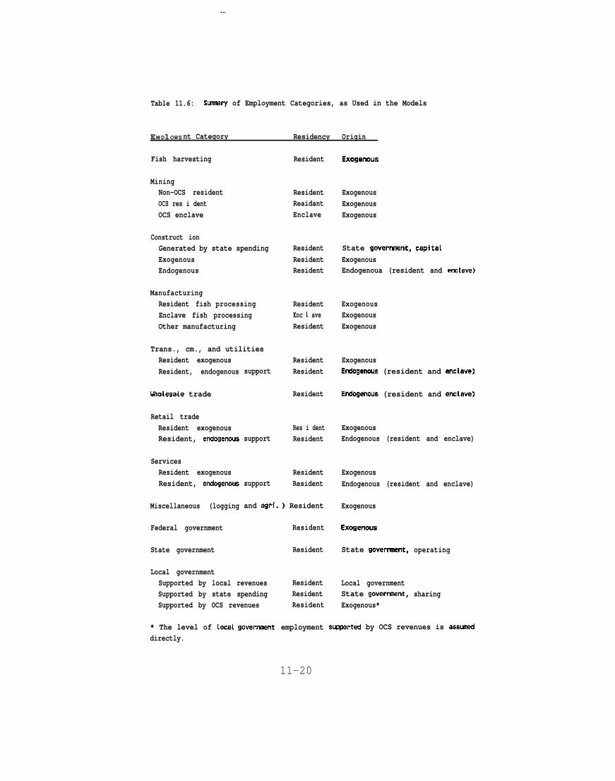
theoretically based upon such a distinction. Table 11.6 shows the

names which we use for different employment categories as they

actually appear and are used in the model, and how they relate to

the categories described in the previous tables.

11-19

.-

Table 11.6: Sumnary of Employment Categories, as Used in the Models

EMD1OWS nt Category Residency Origin

Fish harvesting

MiningNon-OCS residentOCS res i dentOCS enclave

Construct ionGenerated by state spendingExogenousEndogenous

ManufacturingResident fish processingEnclave fish processingOther manufacturing

Trans., cm., and utilitiesResident exogenousResident, endogenous

Uholesale trade

Retail tradeResident exogenousResident, endogenous

ServicesResident exogenousResident, et?dogenous

Miscellaneous (logging

Federal government

State government

Local government

support

support

support

Resident

ResidentReaidantEnclave

ResidentResidentResident

ResidentEnc 1 aveResident

ResidentResident

Resident

Res i dentResident

ResidentResident

and agri. ) Resident

Resident

Resident

Supported by local revenues ResidentSupported by state spending ResidentSupported by OCS revenues Resident

* The level of loca~ goverment employmentdirectly.

11-20

Exoganous

ExogenousExogenousExogenous

State gcwmment, capita~ExogenousEndogenoua (resident and enc!ave)

ExogenousExogenousExogenous

ExogenousEndogenous (resident and enciave)

Endogenous (resident and enctave)

ExogenousEndogenous (resident and enclave)

ExogenousEndogenous (resident and enclave)

Exogenous

Exogemwa

State govemnent,

Local governmentState goverrsnent,Exogenous*

operating

sharing

supfmrted by OCS revenues is assuned

Model Structure

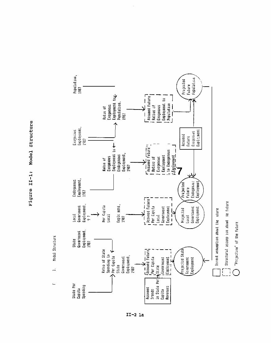
Overview of Model Structure

Figure 11.1 provides a simplified overview of the structure of

the models. The primary measure of economic activity is employment,

measured as annual average employment. Users of the model should be

aware that employment in small coastal Ala”ska communities is highly

seasonal. Thus, depending on the time of year, the actual number of

people working may be considerably higher or lower than annual

average employment. “Average annual employment” provides an average

measure of employment for the whole year, and may bear little

resemblance to the actual employment at any point in time.

Exoffenous em~lovment, by definition, is driven by forces

external to the community. Thus it cannot be ‘Iprojected’t as part of

our models. Instead, we make assumptions about future levels of

exogenous employment, based on expected trends in factors such as

state government spending, fisheries resources, and growth in

tourism. Typically, we base these assumptions on other studies or

the observations of local government officials familiar with plans

and prospects for particular projects and industries.

Endoqenous emRlovment, in contrast, is driven by spending

11-21

.

in r.—— — -1

7 . .I& ——- — -1

al$4‘2Dv+&

.--— —— . \nLk.

.i-.L-WE

0.+u.

.2

L .—— —d \

-1

n

-d’ r-=--lL

11-2 la

internal to

result from

fact, other

employment,

the community, and may be considered to be based upon or

the income generated from exogenous employment. (In

sources of income may also contribute to endogenous

in particular unearned income such as social security.

However, for purposes of simplification, the models assume that all

endogenous employment in a community is “generated” by exogenous

employment) .

We usually assume that the ratios of each category of endogenous

employment to exogenous employment, or the “multipliers,” are fixed.

We calculate these ratios or multipliers from our estimates of

historical endogenous and exogenous employment within each

community. Thus a key part of the model development is estimating

historical endogenous and exogenous employment. We project future

endogenous employment based on these assumed ratios of endogenous to

exogenous employment.

We project local government em~lovment based on an assumed per

capita level of local government employment. We also project state

government em~lovment based on assumed per capita levels of state

government employment. However, assumed per capita state employment

is assumed to decline over time, in proportion to assumed declining

future statewide per capita expenditures as state oil revenues

decline.

II-22

Because the communities are small and our data are limited, in

projecting population wd simply assume that future population will

be proportional to future annual average exogenous employment. We

Figure 11.1

recognize that in the real world~ a great variety of eccnmmicf

demographic, cultural and social factors determine the population of

a community. Although population is usually ultimately linked to

the economic base of a community, many other factors come into play,

such as birth and death rates, and the strength of cultural and

family ties to the community. However, given the lack of data, it

is almost impossible even to document historical birth~ death and

migration’ rates for small Alaska communities, much less to reliably

project them into the future.

In general, we believe it is likely that total employment will

remain roughly in a constant proportion to exogenous employment, and

population will remain roughly in a constant proportion to total

employment. However, during short-term periods of boom or bust,

this assumption may well overstate or understate the actual

population which will occur, as endogenous and government employment

does not in fact adjust immediately to changes in exogenous

employment, and population does not in fact adjust immediately in

proportion to employment. Thus we recognize that our method of

II-23

projecting population is in fact an important simplifying assumption

of the model. However, we do not believe that any more elaborate

approach can be justified by available data.

Below, we provide a more detailed description of the models’

structure and how we developed and calibrated the models. However,

to thoroughly understand the operation of the models we recommend

that users examine the actual worksheet models and trace the

relationships between different cells. To simplify the process of

tracing these relationships, cells which contain numbers which are

directly assumed (for example, exogenous employment and most

historical data) appear in bold upon the screen. Cells which

contain formulas do not appear in bold.

Historical Data

Each model provides employment and population figures for the

years 1980 through 2010. In general, the figures for the years 1980

through 1986 or 1987 are based upon historical data, while the

figures for the years 1986 or 1987 through 2010 are “projections.”

However, for some variables for which data were not available, the

figures for years prior to 1987 were ‘Iprojectedll or inferred based

on other historical data. We used two major sources of historical

data to ‘Scalibratell the model. These were Alaska Department of

II-24

Labor (DOL) data on employment by industry by year, and

miscellaneous data on population for different years.

As our first step in developing the model, we developed

historical employment data for each employment I@category’t (i.e. by

industry, residency, and origin). In general, we began by developing

employment. data by industry, using DOL data wherever available.

13e~artment. of Labor Enmlovment Data. The DOL employment data on

employment by industry by year were based on special computer runs

provided to the Minerals Management Service. As noted above, these

data do not include fish harvesting employment, military employment,

or employment in industries for which there were fewer hhan four

employers (these data were suppressed to guarantee confidentiality) .

The data were provided by the Department of Labor for each quarter.

To calculate annual average employment, we averaged employment over

the four quarters. Where data were suppressed for one or more

quarters, we made our best judgement as to annual average

employment. In general, we used DOL data for historical employment

by industry wherever these data were available.

Other em~lovment data. For industries for which DOL data were

not available (in particular fish harvesting employment and military

employment) we made our best judgement of historical employment

IX-25

using whatever sources were available for each community. These

sources included the 1980 census, planning studies, previous MMS-

sponsored studies, and conversations with city officials.

After developing assumptions on historical

industry, we made further assumptions to divide

employment by

employment within

each industry into different categories, as listed in Table 1X.2.

This involved making our best judgments as to residency and origin

within each industry. In Chapters IIZ-VIII, we describe our

specific assumptions for each industry. Below, we describe the

general approach which

Fish Harvesting.

harvesting.’1 Thus for

we used for each industry.

We usually only measured Itresident fish

most communities we did not attempt to

include “non-resident fish harvesting” as an employment category

within the model.

Locr~inq. Logging employment was assumed only for Yakutat. We

divided logging employment into resident and enclave logging

employment, based on our best judgement as to the share of logging

done by residents.

OCS Mininq.

during the period

No communities were assumed to have OCS employment

1980-1987. Thus these employment categories are

11-26

. . . . . . . . . .

only used for projections.

Construction. Construction was the most difficult industry to

“allocate’~ among different categories of employment. In the absence

of data, we usually divided historical construction employment

primarily between exogenous construction employment, endogenous

construction employment (resident and non-resident) ~ and state-

capital spending construction employment based on a rough judgement

as to the importance of state capital projects and basic industry

capital projects during the period 1980-1987.

Transportation. Communications and Utilities; Retail Trade: and

Services. For several communities; we assumed that some of the

employment in these three support industries was exogenous rather

than endogenous in origin. In other words, we assumed that a

certain share of employment in these industries resulted not from

spending generated within the community but rather from spending

from outside the community. We assigned an exogenous share to

retail trade and services because they cater to tourists as well as

local residents. We assigned an exogenous share to transportation,

communications, and utilities because this industry includes

transportation sezvices for touristis and export/import

transportation via shipping and the Alaska Railroad (for example,

shipments of coal to Korea).

.

Local Government. State government plays an important role in

financing local government in Alaska. A study by the House Research

Agency (“State of Alaska Budget Appropriationsr FY 84-FY 87”) showed

on average that 53 percent of muncipal revenues were from the state,

44 percent were local revenues, and 3 percent were federal in FY 86.

Specifically, state revenues provided 52 percent of of municipal

government funding for Kenai, 40.2 percent for Soldotna (included in

the Kenai market area), 30.8 percent for Kodiak, and 16.9 percent

for Homer. The Finance Director of Cordova indicated that state.

revenues provide 28 percent of municipal funding. State funding

provided an even greater share of funding for school districts in

the study communities. In FY 82, the state share of school district

revenues was 92.6 percent for the Yakutat School District, 82.8

percent for the Cordova School District, 88.6 percent for the Kodiak

School District, and 74.8 percent for the Kenai School District 74.8

(includes Homer, Kenai, and Seward). Based on these figures, we

assumed that a significant share of historical local government

employment in each community was funded by state government

spending.

Summary of Historical Em~lovment Assumptions. Table 11.7

summarizes the assumptions which we used to divide historical

employment in different industries by origin. In many respects this

II-28

division was arbitrary, based upon our best judgment rather than solid

evidence as to what actually supported the jobs. However, we believe

that it is preferable to attempt to divide employment by origin in

this manner rather than to assume origins which are clearly

unrealistic (for example, to assume that all local ltservicesl~

employment is supported by local spending) .

The assumptions are based on very limited information and we

recognize that in fact these shares may well have shifted between the

period 1980 through 1987, rather than remaining constant. For

example, it is quite likely that the actual share of construction

employment supported by state spending rose during the

this period and then fell. However, we have no’ way of

what the actual shares might have been.

We assumed resident shares for employment in fish

first part of

determining

processing of

40 percent for those communities for which data were not available

(Cordova, Kenai and Seward).

We could not determine the actual shares of employment in other

industries which were supported by non-local rather than local

spending. We assumed that the tourism industry is relatively more

important in Homer, Kenai and Seward

Kodiak. Thus we assumed that larger

II-29

than in Cordova, Yakutat and

shares of employment in IJretail

.

trade, “ “services” and “transportation, communication and utilities”

were exogenous in these communities.

For all of the communities, we assumed that 50 percent of local

government employment was supported by local revenues and the

remainder by state revenue sharing.

11-30

.

Table 11.7: Sumnary of Assqt ions Used in Developing Historical En@ oymant Aasmpt i ons, by Comuni ty

Assunad Shares of Historical Employment

Wlolomant Category Cordova Homer Kanai Kodiak Seward Yakutat

Conatructi onGeneratad by state spendingExogenousEndogenous

ManufacturingResident fish processingEnclave fish process i ng

Trans., cm., arxi utilitiesResident exogenousResident, endogenous support

Retai 1 trsdeResident exogenousResident, endogenous support

ServicesResident exogenousResident, endogenous su~rt

Local governmentSupported by 1 oca 1 revenuesSupported by state spending

a 25.25.,50

.40

.60

.05

.95

.05

.95

.50

.50

.25

.25

.50

.79

.21

.10

.90

.25

.75

.10

.90

.50

.50

.25

.25

.50

.40

.60

.10

.90

a 25.75

.10

.90

.50

.50

.25a 25.50

.47

.53

.05

.95

.10

.90

.05

.95

.50

.50

.25

.25

.50

.40

.60

.10

.90

.25

.75

.?0

.90

.50

.50

.25

.25

.50

.25

.75

.05

.95

.10

.90

.05

.95

.50

.50

Historical Population

Sources of information on population during the period 1980-

1987 were limited. The major sources were the 1980 U.S. census, the

Alaska Department of Labor, “Alaska Population Overview” and the Kenai

Peninsula Borough, “Situation and Prospects.’t

The ItAlaska Population

IX-3 1

Overview” and “Situation and Prospects” are both published annually,

so several issues of each were used. In addition, the several city

planning departments provided local population estimates, including

population outside the city limits but in the vicinity of the city.

Projections

We term the employment and population figures in the models for

the years 1987-2010 “projections.i’ Below, we describe how we arrive

at these projections.

Exoaenous Emnlovment. As noted above, we assume future levels

of exogenous employment, based on expected trends in factors such as

state government spending, fisheries resources, and growth in

tourism. Typically, we base these assumptions on other studies or

the observations of local government officials familiar with plans

and prospects for particular projects and industries. In Chapters

III-VIII, we describe how we arrived at the assumptions for each

exogenous employment category. The exogenous employment assumptions

are critical to the model for two reasons. First, exogenous

employment represents approximately half of total employment. Thus

we are directly assuming half of our “projections.” Secondly, our

exogenous employment assumptions “drive” our projections for

endogenous and government employment and population.

11-32

. . . . . .

Endoqenous em~lovment. Endogenous employment includes all or

part of employment in five industries: transportation, ~ommuni-

cations and utilities; wholesale trade; retail trade; finance,

insurance and real estate; and services. We project future

endogencms employment in these industries by projecting future total

end’ogenous employment and then dividing this total into (usually

fixed) shares, based on past trends (usually our historical figures

for 1986 or 1!387). Table 11.8 compares our assumptions of the share

of total future endogenous employment assumed for each industry in

each community.

11-33

,.

Table 11.8: Sunnary of Assumptions for Projections of Future

Endoganous and Goverment En@oyees

Cordova Hcmer Kens i Kodiak Seward Yakutat

Share of Total Endogenoua E@oynientconstruct ionTrans., Cm., and Util.Uholesale TradeRetai 1 TradeFinance, Ins., and ReaL EstateServices

Endogenous Emp( oyment Multi pliers[EMEDREEX87/EMREEX871

Local Goverment En’ploymantMultiplier [EMEGLR87/ENEXT 1981

Base State Goverment EmploymentHultipl i er [EMSG87/EMEXT0871

Base State-Sufqxmted ConstructionEn@oymant Multiplier[EMCOSS87/EMEXT0874

Base State- Sup@rted LocalGovermant Enploynent Multiplier

.04

.21

.05

.37

.07

.26

.82

.20

.15

.01

.08

.03

.21

.04

.33

.08

.30

.97

.23

e 03

.03

.23

.07

.10

.09

.32

.06

.361.68

.22

.21

.04

.22

.06

.12

.03

.40

.06

.33

.51

.06

.06

.01

.06

.10 .02

.11 .26

.09 .02

.26 .31

.04 .12

.39 .261.18 .99

.15 .20.

.36 .08

.17 .00

.15 .20

[Note that state supported construct ion for Yakutat was shown as 0.1

We project total endogenous employment as follows. First, we

divide total endogenous employment by origin, into resident-

generated and enclave-generated categories. We assume a fixed

employment multiplier of .05 for enclave-generated endogenous

employment. In other words, we assume that every 100 enclave

workers generate 5 endogenous employment jobs. This is a

II-34

.

deliberately low multiplier reflecting a very low local economic

impact of enclave workers. It is an important model assumption

however, because of the significant number of enclave workers which

might accompany future OCS development. The choice of enclave

multiplier directly affects the size of tihe projected impacts of oCS

development.

Based on this multiplier? we calculate assumed enclave-

generate”d endogenous employment for the period 1980-1987, and

subtract this figure from total endogenous employment to arrive at

resident exogenous employment-driven endogenous employment for the

period 1980-1987. We project future resident exogenous employment-

driven endogenous employment by assuming that it changes from the

1987 level in proportion to changes in resident exogenous employment.

Our methodology for projecting future endogenous employment may

be summarized as follows:

EMEDTO = EMEDREEX i- EMEDEN

EMEDEN = .05 x EMEN

EMEDREEXt = EMREEXt X [EMEDREEX87/EMREEX87]

11-35

. . . ,--

where

EMEDEN = Endogenous employment driven by enclave employment

(Employment EnDogenous ENclave)

EMEDREEX = Endogenous employment driven by resident exogenous

employment (Employment EnDogenous REsident

EXogenous)

EMEDTO = Total endogenous employment (Employment EnDogenous .

TOtal )

EMEN = Enclave employment (Employment ENclave)

EMREEX = Resident exogenous employment (Employment REsident

EXogenous)

The expression [EMEDREEX87/EMREEX87] may be viewed as a

“multiplier “ for resident exogenous employment-driven endogenous

employment. Table 11.8 summarizes the values which we assumed for

this multiplier in each model.

Government EmDloyment. We project local government employment

supported by local tax revenues by assuming that it changes from the

II-36

1987 level in proportion to changes in total exogenous employment.

This is similar to our approach for projecting endogenous employment

except that it is based on total exogenous employment rather than

resident exogenous employment. In effect, we are assuming that

local tax revenues are proportional to total (resident and enclave)

exogenous employment.

Our methodology for projecting local government employment

supported by local tax revenues may be summarized as follows:

EMLGLRt = EMEXTOt X [EMLGI.R87/EMEXT087]

where

EMLGLR = Local government employments supported by local tax

revenues (Employment Local Government supported by Local Revenues)

EMEXTO =

TOtal )

Total exogenous employment (Employment EXogenous

The expression [EMLGLR87/EMEXT087] may be viewed as a

“multiplier II for local government employment supported by local tax

revenues. Table 11.8 summarizes the values which we assumed for

this multiplier in each model.

rI-37

The other categories of government employment in our model are

supported by state spending (including construction employment

supported by state capital spending). For all of these categories,

we assume that employment changes not only in proportion to the size

of the community economic base (as measured by total exogenous

employment) , but also in proportion to per capita state spending,

resulting from changes in per capita state revenues. Our

assumptions for future state per capita spending are shown in Table

II-9 . These assumptions are based on projections from ISER’S

statewide MAP econometric model.

Our methodology for projecting other categories of government

employment may be summarized as follows:

EMSGt = EMEXTOt X [EMSG87/EMEXT087] X [STPCOPEXt/STPCOPEX87]

EMLGSSt = EMEXTOt X [EMLGSS87/EMEXT087] X [STPCOPEXt/STPCOPEX87]

EMCOSSt = EMEXTOt X [EMCOSS87/EMEXT087] X [STPCCAEXt/STPCCAEX87]

where

EMSG

Government)

= State government employment (Employment State

II-38

.

Table II-9: Derivation of State Per Capita Operating and CapitalExpenditure Assumptions

State State Per capita Per capitaState operating capita 1 operating capita~popdation expenditures expenditures expandi tures expandi tures

Year (thousands) ($ mil[ions) ($ millions) ($ thousarxis) ($ thousands~

198019811982198319841985

1987198819891990199119921993199419951996199719981999200020012002200320042005

20072008200920102011

420435461495523540536536529524528528532535538547552555564573581588594604612620636652662677691706

1253 3281564 4671983 5582239 5492255 6512295 8242308 6522308 ‘ 6521965 4121743 2461836 3241790 3161894 3341888 3331778 3131976 348!953 3441795 3162054 3622!25 3752015 3551932 3411833 3231948 343188s 3331860 3281837 3241833 3231802 3181968 3471941 3421888 333

11-39

2.993.604.304.524.314.254.314.313.713.333.483.395.563.533.313.(5!3.543.233.653.713.473.293.093.233.093.002.892.812.722.912.812.67

0.781.071.21l.l?! .241.531.221.220.780.470.610.600.6.30.620.580.640.620.570.640.650.610.580.540.570.540.530.510.500.480.510.490.47

EMLGSS = Local government employment supported by state

spending (Employment Local Government State Spending)

EMCOSS = Construction employment supported by state spending

(Employment Construction State Spending)

ST’PCOPEX = State per capita operating expenditures (STate Per

Capita OPerating Expenditures)

STPCCAEX = State per capita capital expenditures (STate Per

Capita CApital EXpenditures)

EMEXTO = Total exogenous employment (Employment EXogenous

TOtal )

The expressions [EMSG87/EMEXT087], [EMLGSS87/EMEXT087]”, and

[EMCOSS87/EMEXT0~,] may be viewed as a ‘Imultipliersi’ for these

categories of state-government supported employment. Table II-8

summarizes the values which we assumed for these multipliers for

1987 for each model. However, in subsequent years, we adjust the

effective multipliers downwards as state per capita spending

declines.

11-40

Population. We project future resident population by assuming

that it changes in proportion to resident exogenous employment. Our

methodology for projecting future population may be summarized as

follows:

I?cmt = EMREEXt X [PORE87/EMREEX87]

where

PORE = Resident Population (Population REsident)

EMREZX = Resident, exogenous employment (Employment REsident

EXogenous)

The expression [PORE87/EMREEX87] may be viewed as a ‘multip-

lier” for population. Table 11.8 summarizes the values which we

assumed for this multiplier in each model. In order to calculate

population by age group, we assume that the resident population age

distribution remains the same as in the most recent year for which

age distribution data are available (generally 19S0, from the 1980

U.S. Census).

We do not distinguish between Native population and non-Native

population except for the Yakutat model. In the Yakutat model, we

IT-41

assume that Native population grows at a constant growth rate but

cannot exceed 70 percent of total population. Non-Native population

is projected as described above.

II-42

CHAPTER III. DESCRIPTION AND MODEL

Cordova

Sound, about

northwest of

Overview

is located near the

160 miles southeast

eastern

ASSUMPTIONS: CORDOVA

entrance to Prince William

of Anchorage and about 410 miles

Juneau. Valdez is 65 miles to the northwest across

Prince William Sound. The community fronts on Prince William Sound

and is adjacent to Chugach National Forest. Cordova is accessible

by air and water. Plans have been made to connect it with the

state (over land) highway system by completing the Copper River

Highway. Before the 1964 earthquake, construction of the highway

was completed to Mile 59. After the earthquake destroyed bridges,

the project was reconsidered, and today only a temporary route

exists as far as mile 52.

Cordova, with a population of about 2,510, is dominated by

commercial fishing and seafood processing. During summer months

the community’s population may almost double due to the influx of

transient workers. Fishing and fish processing is estimated to

account for 50 percent of local employment (Cordova Draft

Comprehensive Plan).

III-1

,.,E

.— -----—---- . . . ---. ..-. a .x”b. ..” “:.=.-z -~

( H.LHON

+S311N

III-l(a)

Government is the second most important sector in the economy,

providing stable year-round employment. Tourists visiting the

community generally come to hunt or fish. Tourism is regarded as

having expansion potential.

Employment in Cordova peaked in 1982, although higher

employment occurred in transportation, communications, and

utilities and local government during 1982-1984 due to several

public construction projects (a small boat harbor expansion,

construction of the north and south containment area and a new

hospital) .

Maior Data Sources

The primary data source for our analysis of Cordova was

Department of Labor data on employment for Cordova. In addition we

used an unpublished 1983 study by the Institute of Social and

Economic Research (ISER) “Cordova: Present and Projected Levels of

Population, Employment, and Income.Jf We also talked to Carla

Moore, a city planner for Cordova and Dale Daigger, the City

Finance Director. We have listed all of the sources used in our

analysis at the end of this chapter.

III-2

Studv Area

Figure 111.1 shows the area which we are defining as

“Cordova.” Our employment and population assumptions and

projections for this study refer to employment and population

within this area. This includes the road-connected area around

Cordova and corresponds to the Issub-sub arealg used by Department of

Labor for employment statistics.

Emplovment Assum@ions

Table 111.1 shows Alaska Department of Labor average annual

employment data for Cordova for the years 1980-1987. An asterisk

“*” indicates that the figure is not available because the figures

were suppressed for one or more quarters. These data formed the

primary basis for the development of our employment assumptions,

and are the basis for all employment’ data not otherwise cited.

We made additional assumptions to account for industries not

included in the Department of Labor data (eg. fish harvesting) or

which were fully or partially suppressed (eg. manufacturing and

wholesale trade) , and to allocate employment within a given

industry between resident and enclave shares, exogenous and

endogenous shares, etc. Our resulting employment assumptions for

III-3

the years 1980-1987 are shown in Table 111.2. Below we discuss

these assumptions by industry.

Table 111.1: Wmnary of Department of Labor Employment Data for Cordova

Cateraory Cede 1980 1981 1982 1983 1924 1985 1986 198?

MiningConstruct ion14anufacturingTrans., COIM’I., UtilitiesWholesale TradeRetai 1 TradeFin., Ins., & Real EstateServicesForestry, Ag., FisheriesFederal GovernmentState GovernmentLoca 1 GovernmentTOTAL

1 0 0 0 0 0 0 0 02 17 22 30 26 34 37 25 *

3 * * * * * 263 * *4. 117 185 261 242 189 78 70 795 * * ● ● * * * *6 132 151 177 163 141 154 140 1437 25 26 24 23 23 25 25 268 111 105 122 124 113 102 103 969 * * * ● ● * * *

10 35 42 37 34 32 30 30 3111 81 87 87 88 92 96 96 8912 167 179 192 197 181 174 166 162

828 1071 1175 1180 * * * *

*Data suppreasd.

III-4

Table 111.2: Sumnsry of Employment Assqtions for Cordova, 1980-1987

Fish harvestingMining

Non-OCS residentOCS residentOCS enclave

Construct ionGenerated by state spendingExogenousEndogenous

Manufecturi ngResident fish processingEnclave fish processingOther manufacturing

Transportation, comn. and utilitiesExogenousEndogenous

Wholesale tradeRetai i trade

ExogenousEndogenous

Finance, Insurance and Rest EstateServices

ExogenousEndogenous

M i sce 1 [ aneousLogging

Federat govermentState goverrmnantLocal governmentSu~rted by local revenuesSu~rted by state spendingSupported by OCS revenues

Tota L

Fish Hanestinq

1980 1981 1982 1983 1984 1985 1986 1987186

000017449

277111166

0117

611116

13213

11925

1116

1051010928116767

1000

1231

Cordova is the center

1860000

2266

1127?111166

01859

17619

15115

13626

1055

1001010998717972107

0

1346

wo000

3088

15277111166

026113

2482217718

159241226

1161010948719277

1150

1482

of fishing

1860000

2677

13277!11166

024212

2302016316

14723

1246

11810109188

19779

1180

1447

1860000

349917

277111166

01899

18017

14114

12723

1136

10710108992

18172

1090

1352

1860000

3799!9

263105158

0784

7419

15415

13925

1025

9710108796

17470

1040

1231

1860000

2566

13263105158

0704

6717

14014

12625

1035

981010879616666100

0

1188

1860000

2566

13263105158

0794

7518

14314

12926965

9110108889

162117450

1185

and fish processing for an

area encompassing 38,000 square miles of Prince William Sound and

the Copper River and Bering River fisheries. Fishing employment is

cyclical. It begins to increase in March with the herring fishery

and peaks in August with salmon. In the ADFG Area E Fishery

(Prince Wiiliam Sound), Cordova residents hold 222 of 545 drift net

permits and 125 of 271 seine permits.

There are no Department of Labor employment estimates for fish

harvesting employment. The 1980 federal census showed 174 employed

pesons claiming forestry, fishing or farming as an occupation. Most

would have been employed in fishing. However,

data were collected for the last week of March

the federal census

1980, but this may

have reflected the situation later in the spring. Therefore, we

estimate a ‘Sseasonality factor” by comparing Alaska Department of

Labor employment data for manufacturing in the second quarter of 1980

to average annual employment for the entire year. The resulting

seasonality factor is 277/260 = 1.07. It is assumed that the

seasonality of fishing employment is similar to that of manufac-

turing. Multiplying the census figure of 174 by the seasonality

factor of 1.07 results in employment (FTE) of 186 in 1980. We have

assumed this figure for the period 1980-1987. We have also assumed

that fish harvesting employment will remain constant at this level

for the period 1988-2020.

III-6

Mininq

Non-OCS Resident. Katalla Field, a small field discovered in

1902, operated for 3CI years but produced only 154,000 barrels of

oil. The Alaska Crude Corporation has been investigating the poten-

tial of the Katalla fields, but work is at a standstill, probably

largely due to the decline of world oil prices. Construction of a

road, unlikely in the current state economy, linking oil fields to

the Copper River Highway would improve the feasibility of this

project. However, direct employment benefits would be limited

because it is a small oil field. The possibility of selling oil and

gas to the local electric cooperative for use in generating

electricity has been proposed.

The Bering River coal fields were discovered in 1896. However,

withdrawal of Alaska’s coal lands in 1906 prevented exploitation.

The Chugach Natives, Inc. and KADCO, lncm (a Korean fire) have

identified 62 million tons of anthracite coal in the eastern part

of the Bering River coal fields. However, 32 miles of road would

need to be constructed in order to develop this coal resource. If

access were available, the magnitude of potential economic benefits

to Cordova still would depend to a great extent on the location of

an export facility. Another possible benefit of developing this

coal resource may be cheaper fuel for the local electric

111-7

cooperative. Wheelabrator Coal Services Company has completed a

prefeasibilty study of this project (Assessment of the Feasibility

and Implementation of Port and Transportation System Alternatives

for the Bering River Coal Field). Although it is projected that

245 people would be directly employed if this resource were to be

developed, the report states that it is not a feasible project at

this time due to low market

it is feasible only under a

There is currently no

the Cordova area. We thus

for the period 1980-1987.

1

i

price and high development costs, i.e.,

most optimistic, unrealistic scenario.

aining or mineral extraction occurring in

assume that mining employment was zero

We also assume that onshore mining employment remains at zero

for the period 1988-2020. Essentially, this is an assumption that

development of the Bering River Coal Field does not occur.

OCS Mininq. Exploration following a 1976 federal OCS lease

sale in the northern Gulf of Alaska resulted in little direct

economic impact in Cordova. We have assumed zero OCS mining

employment in Cordova during the period 1980-1987. Our “base case”

model assumptions similarly assume zero OCS mining employment during

the period 1988-2020.

III-8

Miscellaneous

Loau incf.. Eyak Corporation is hamesting 10-20 truck loads a day

of timber which is shipped out of the community. We have assumed

employment of 10 in logging for the period 1980-1987. We assume

employment of 10 in logging for the period 1988-2020.

Construction

Cordova

construction

would receive a large influx of public money and

jobs if either the Copper River Highway were completed

or the Katalla Road were built. Copper River Highway completion

would take an estimated 10 years. Given

situation, we assume that this road will

The Alaska Department of Labor data

employment increasing from 17 in 1980 to

the state’s current fiscal

not be built.

show Cordova construction

37 in 1985 and then

dropping to 25 in 1986. We assumed the same figure of 25 for 1987,

which was suppressed in the Department of Labor data.

We assumed that 25 percent of construction employment during the

period 1980-1987 was supported by state government capital spending,

25 percent was exogenous, and 50 percent was endogenous, based on our

111-9

best judgment in the absence of any data.

We assumed exogenous

2020 based on on our best

employment of 6 during the period 1988-

judgment in the absence of any data.

Manufacturing

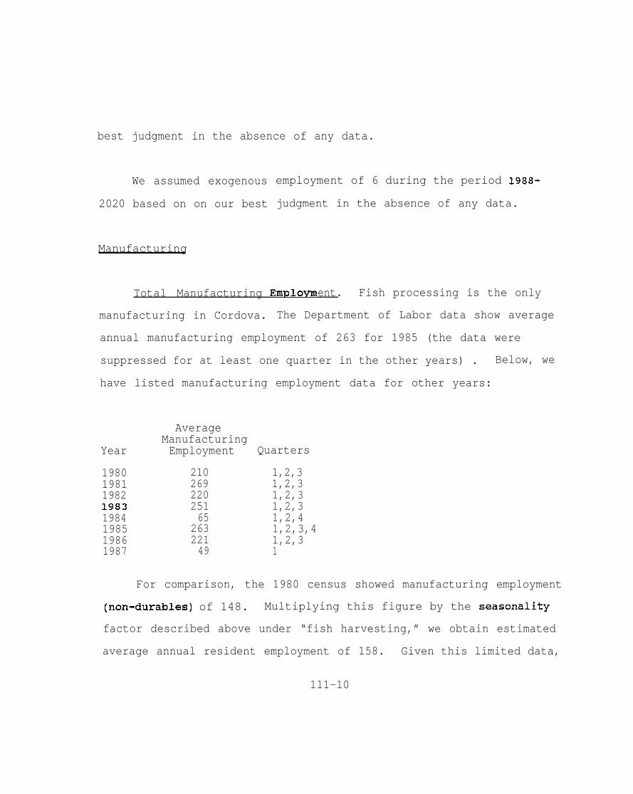
Total Manufacturing EmDlovment. Fish processing is the only

manufacturing in Cordova. The Department of Labor data show average

annual manufacturing employment of 263 for 1985 (the data were

suppressed for at least one quarter in the other years) . Below, we

have listed manufacturing employment data for other years:

Year

19801981198219831984198519861987

AverageManufacturingEmployment

21026922025165

26322149

Quarters

1,2,31,2,31,2,31,2,31,2,41,2,3,41,2,31

For comparison, the 1980 census showed manufacturing employment

(non-durables) of 148. Multiplying this figure by the seasonality

factor described above under “fish harvesting,” we obtain estimated

average annual resident employment of 158. Given this limited data,

111-10

we assumed total fish processing employment of 277 in 1980 through

1984 and 263 for 1985-1987.

Resident and non-resident fish Drocessinq. The Cordova city

planner that we contacted suggested that 75 percent of fish

processing employment is non-resident. She indicated

number of cannery workers are Filipinos from Hawaii.,/

percent resident share for fish processing employment

that a visible

We assumed a 40

during the

years, 1980-1987, which resulted in an assumption of resident fish

processing employment of 111 for 1980-1984 and 105 for 1985-1986.

Non-resident fish processing employment is thus assumed to be 166

during 1980-1984 and 158 for the period 1985-1987.

We assumed that both resident and non-resident fish processing

employment will remain constant at their 1987 levels during the

period 1988-2020.

Transportation. Communications, and Utilities

The Department of Labor average annual employment figures for

transportation, communications and utilities range from 117 in 1980 to

about 261 in 1982. Employment declined to 189 in 1984 and 78 in

1985. We assumed that 5

exogenous and 95 percent

percent of employment in this industry was

was endogenous. We assumed that exogenous

111-11

transportation, communications and utilities employment will grow at

3 percent per year after 1987, based on an assumption that tourism in

the Cordova area will grow at a rate of 3 percent per year.

Wholesale Trade

Wholesale trade figures were suppressed by the Department of

Labor. However, according to the ISER study, in 1980 wholesale

trade employment was 11 percent of total trade (based on employment

data from the 1980 census). We assumed that wholesale trade during

1980-1987 was 11 percent of total trade, or 12 percent of retail trade

employment. This results in estimates of wholesale trade employment

ranging from 16 in 1980 to a high of 22 in 1982. We assumed that all

wholesale trade employment was endogenous.

Retail Trade

Department of Labor average annual employment figures were used

for the retail trade category. These ranged from 132 in 1980 to 177

in 1982, 141 in 1984, and 143 in 1987 (Table 111.1). We assumed that

10 percent of retail trade employment was exogenous and 90 percent

was endogenous. We assume that exogenous retail trade employment

will grow at a rate of 3 percent per year after 1987.

111-12

Finance, Insurance, and Real Estate

Department of Labor annual average employment figures were used

for this category (Table X1X.1). ‘~FIRE8e employment remained

relatively constant during the stiudy period, varying between 25 in

1980, 23 in 19$3 and 1984, and 26 in 1987. This category was assumed

to be entirely endogenous.

Services

We used

o

Department of Labor annual average employment figures

for our employment assumptions in all of these industries. We

assumed that 5 percent of employment in this industry was exogenous

and 95 percent was endogenous. We assume that exogenous services

employment will grow at a rate of 3 percent per year after 1987.

Federal Government

Civilian federal government employment in Cordova increased from

35 in 1980 to 42 in 1981 and then declined to 30 in 1985 and 1986

(Table 111.1). The Coast Guard maintains one unit at Cordova with

57 personnel. Other federal agencies with offices in Cordova include

the U.S. Forest Service, the Post Office, and the Federal Aviation

Administration. Total federal government employment is projected at

111-13

88 during 1988-2020.

State Government

State employment increased from 81 in 1980 to 96 in 1985 and

1986 then declined to 89 in 1987. State offices in Cordova are the

Department of Public Safety, Department of Fish and Game, the Court

System, and the University of Alaska, Alaska Marine Advisory Program.

Local Government

Total local government employment grew from 167 in 1980 to

197 in 1983, then declined to 162 in 1987. The city provides

education, recreation, public safety services, roads, water, sewer,

snow removal, and alcohol and mental health counseling. Facilities

maintained by the city include city hall, the city shop, the

hospital, the port and harbor, a sanitary landfill, a sewage disposal

plant, streets and roads, and water storage tanks and reservoirs.

The finance director, City of Cordova, estimated that currently local

government is supported 28 percent by state funding. According to

the Alaska State Legislature, House Research Agency (Report 87-A), in

FY 1982, 82.8 percent of revenues for the Cordova School District

came from the state. Comparing these two figures, and based on our

best judgment, we assume that state revenues support 50 percent of

111-14

total local government.

Table I I 1.3 Estimated E@oynent in Cordow

1980 1981 1982 1983 1984 1985 1986 1987

Resident Sasi cFishingFish Processing14iscel laneoua-LoggingOther {mining, manufacturing)

Resident SupportExogenousEndogenousGovernment SponsoredEnclave Sponsored

Resident GovernmentExogenousEndogenous

TotaL ResidentTotal ExogenousTotal Endogenous

Non-Resident (Enclave) Employment

Total Resident plus Non-Resident

307186111100

41829

3854

34092

248

1065428637

166

1231

307186111100

508’35467

6

36599

266

1180441n9

166

1346

307186111100

63644

5848

m94

279

1.316445871

166

14a2

307186111100

59841

5507

37691

285

1281439842

166

1447

307186111100

51738

4719

36289

273

1184434752

166

1352

301186f 05100

41534

3729

35787

270

1073422651

158

1231

301186105100

38029

3456

34987

262

1030417613

158

1188

Emnlovment Multipliers

Table 111.4 summarizes employment lrmultipliers$l for the

301186105100

38729

3516

339m

251

1027419609

158

1185

period 1980-1987. In general, these multipliers remain relatively

constant, except for the Endogegous Employment Multiplier, which

was higher during the period 1981-1984 when more construction

111-i5

projects occurred.

Table 111.4: Summary of Employment Multipliers, 1980-1987

1980 1981 1982 1983 1984 1985 1986 1987

Endogenous En@oyment Multipliers[EMEDREEX/EMREEXl

Loca 1 Goverrnh?nt Enpl oymantMultiplier [EMLGLR/EMEXTO1

State Government EniploymentMuL t ipl ier [EMSG/EMEXTOl

State-Supported ConstructionMultiplier [EMCOSS/EMEXTOl

State- Suppated Loca~Government Employment Multiplier[EMLGSS/EMEXTOl

0.88 1.04 1.29 1.24 1.07

0.11 0.12 0.13 0.13 0.12

0.14 0.14 0.14 0.15 0.15

0.01 0.01 0.01 0.01 0.01

0.17 0.18 0.19 0.20 0.18

POT3UlZitiOn ASSUIIIDtiOIE

0.86

0.12

0.17

0.02

0.18

0.81

0.12

0.17

0.01

0.17

0.82

0.20

0.15

0.01

0.08

Table 111.4 summarizes available population data for Cordova for

the period 1980-1987, as well as our population assumptions for this

period. Our 1980 assumption for total population was based on the

1980 census. The source of the population figures for 1981 through

1983 was the “Alaska Population Overview.” The source for years

1984-1987 was the City of Cordova.

Population outside of the city limits but within the area served

by roads from Cordova is shown at 441 by the city for 1983 through

111-16

1987. A planner with the city said that development of these

outlying areas began in the late 1970’s. She indicated that the

population had remained relatively constant during this decade.

Thus, we hold. the figure constant at 441.

Our age distribution assumptions are based on the 1980 census.

We assume that this age distribution remains constant throughout the

projection period.

e

The ratio of assumed resident population to assumed resident

exogenous employment increased from five in 1980 to seven in 1987.

The fact that this ratio increased suggests that-the availability of

work has decreased.

111-17

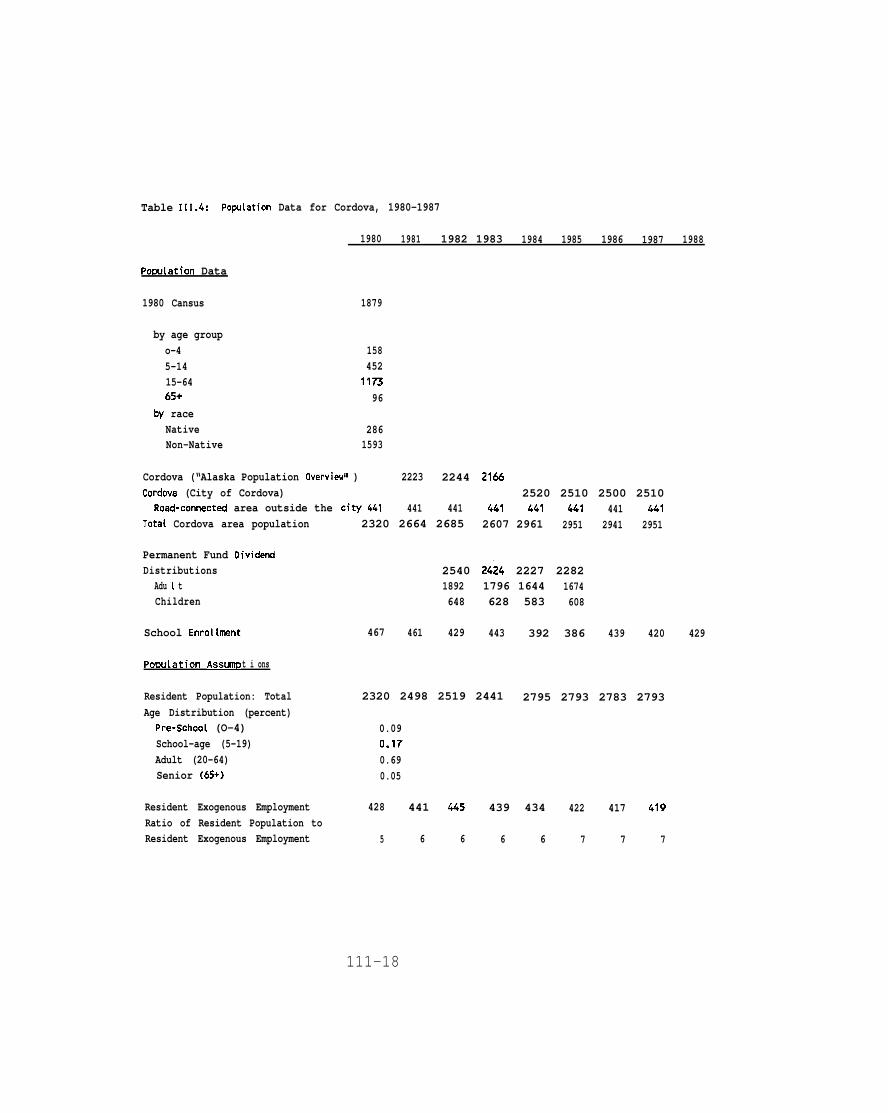
Table 111.4: Po~lation Data for Cordova, 1980-1987

1980 1981 1982 1983 1984 1985 1986 1987 1988

Pomtation Data

1980 Cansus 1879

by age groupo-4 1585-14 45215-64 1!7365+ 96

by raceNative 286Non-Native 1593

Cordova (“Alaska Population Ovarvieu” ) 2223 2244 2166Cordova (City of Cordova) 2520 2510 2500 2510

Rosd-connected area outside the city 441 441 441 441 441 441 441 441Totat Cordova area population 2320 2664 2685 2607 2961 2951 2941 2951

Permanent Fund OividetiDistributions 2540 24;4 2227 2282

Adu 1 t 1892 1796 1644 1674Children 648 628 583 608

School Enro{[ment 467 461 429 443 392 386 439 420 429

Powlation ASSUIIR t i ons

Resident Population: Total 2320 2498 2519 2441 2795 2793 2783 2793Age Distribution (percent)

Pre-School (O-4) 0.09School-age (5-19) 0.17Adult (20-64) 0.69Senior (65+) 0.05

Resident Exogenous Employment 428 441 445 439 434 422 417 419Ratio of Resident Population toResident Exogenous Employment 5 6 6 6 6 7 7 7

111-18

Base Case Projections

Figure 111.2 and Table 111.6 summarize our base case projections

for Cordova. Total population rises slightly over the projection

period. This is due primarily to increasing tourism.

111-19

Figure III-2: Cordova Base Case Projections

,:Q ~~~,/~

BASE CASE Etvi PLCIYhfENT ANtI PCIPUL4TION3,2 !3-I Tgtal p@pula~@n

2.8

}~

/

~v 6 -# eelden Population‘A

2s4 /

,

k

2<2

2

1,8

1,6 1

!~-‘“4 ,%(%1,~

<Total Employ-nor-i

1Reslcbnt Employment

0,8

0.6 + I

o I I I I I I i I1980 1905 1 SW 1*5 2000 20M 2010 2015 2020

‘fl%R

111-20

Tab~e 111.6: Smry of Employment and Po@ation Projections for Base Case

EMPLOYMENT POPULAT IONTotal,

Enc 1 ave Res i dentResident Resident Resident Fish- Enc Lave Enclave and

Year Non-OCS Ocs Total Process. Ocs Tota 1 Enclave Resident Enclave Tota 1198019811982198319841985198619871 98a1989199019911992199319941995199619971998199920002001

200320042005200620072008200920102011201220132014201520162017201820192020

1065118013161281118610731030102710079951002100110081009100310151015100710221026102110171013102010181017101610161016102510251028103110341037104010441047105110551059

00000000000000000000000000000000000000000

1065118013161281118610731030102710079951002100110081009100310151015

10221026102170171013

10181017101610161016102510251028103110341037

10441047105110551059

166166166166166158158158158158158158158158158158158158158158158158158158158158158158158158158158158158158158158158158158158

00000000000000000000000000000000000000000

lM

166166166166158158158158158158158158158158158158158158158158158158158158158158158158158158158158158158158158158158158158

123173461482144713521231!1881185llti11521159115811651166116111731172116411801184117811751170117711751175117411741174118311821185118811911195119812011205120912121216

23202498251924472795279327832793273927062725272227422744272927612760273827802792277727662755277427682767276427642764278827872795280328122821283028392849285928692880

166166166166166158158158158158158158158158158158158158158158158158158158158158158158158158158158158158158158158158158158158

2486Z&268526072961295129412951289628632883287928992901288729182917289629382950293429242912293129252924292229222921294629442952296129692978298729973006301630273037

111-21

References

Alaska Department of Labor, Alaska Po?mlation Overview 1985Estimates, April 1987.

Alaska Department of Labor, Employment Database Files forCordova, Homer, Kenai, Kodiak, Seward, and Yakutat, November1988 (unpublished).

Alaska Department of Labor, Geoclra~hical Area ClassificationManual. January 1981.

Alaska Department of Labor, July 1 Population Estimates, NewsRelease, March 1, 1988.

Alaska Department of Revenue, Permanent Fund Dividend RecipientProfiles.

Cordova, City of, Draft Comprehensive Plan, Funded by AlaskaCoastal Management Program, January 1988.

Keiser, Gretchen, and Pierce, Brad. State of Alaska Budcret, FY 84-FY 87. Alaska State Legislature, House Research AgencyReport 87-C, February 1987.

Knapp, Gunnar; Nebesky, Will; and Hull, Teresa. Cordova: Presentand Proiected Levels of Pormlation. Em~l oyment, and Income.University of Alaska, Institute of Social and EconomicResearch, March 1983 (unpublished draft report prepared forMinerals Management Service, Alaska OCS Office).

Livey, Jay, and Keiser, Gretchen. Public School Financina inAlaska. Alaska State Legislature, House Research AgencyReport 87-A, February 1987.

Moore, Carla. City of Cordova. Telephone Interview, October 28,1988 and December 1, 1988.

U.S. Census, 1980.

III-22

CHAPTER IV. DESCRIPTION AND MODEL ASSUMPTIONS HOMER

Cook

. juts

air,

Overview

Homer is located near the entrance of Kachemak Bay in lower

Inlet. It is unique with its 5 mile sandspit peninsula that

halfway across Kachemak Bay. Homer is accessible by highway,

and water. Homer is about 225 miles by highway south of

Anchorage. It is a 40 minute flight from Anchorage with flights

available from three air lines. Homer is also accessible by the

Alaska Marine Highway System ferries or on one of several cruise

ships.

Homer, with a

commercial fishing

population of about 4,000, is dominated by

and seafood processing. Over 400 fishing

vessels use Homer as a base of operations fishing for herring,

crab, halibut, and salmon, as

fish.

Government is the second

stable year-round employment.

well as vessels fishing for bottom

most important employer, providing

Tourism and

important part of the economy. According

Iv-1

recreation are also an

to City of Homer Compre-

hensive Plan (1983), Homer had a growing population of retired and

“commuting “ households--households with primary residences in

Homer but jobs elsewhere (i.e., north slope workers, pilots,

etc.) . Homer has historically gained population in advance of

economic growth and creation of job opportunities which then tend

to ‘&catch up’R with the population over time. Tour boats have

begun stopping

The Homer

in Homer.

area has gained employment since the start of

construction on the Bradley Lake Hydropower Project in 1987.

Bradley Lake hydropower construction project has utilized marine,

staging and transportation services out of Homer. However, since

the project was just gearing up in 1987, historic data do not

reflect a large increase due to Bradley Lake employment.

Total employment in Homer declined between 1984 and 1987.

Construction employment increased in 1984-1985 due primarily to a

new (DECRA) home loan program. Other construction projects during

the 1980’s included a fish dock in 1980-1981, and a $5 million

high school in 1985-1986.

Maior Data Sources

The primary data source for our analysis of Homer was

IV-2

Department of Labor data on employment for Homer. In addition we

used Gulf of Alaska Economic and Demoara~hic Svstems Analvsis,

Minerals and Management Service, Technical Report 98 (TR 98)

(March 1984) and Commercial Fishina Industrv Studv Homer, Alaska,

University of Alaska Marine Advisory Program, Douglas D.

Coughenower (November 1987). We also talked to Pam Black and

Eileen Bechtol, planners with the City of Homer. We have listed

all of the sources used in our analysis at the end of this

chapter. “

Studv Area

Figure IV.1 shows the area which we are defining as “Homer.”

Our employment

study refer to

corresponds to

and population assumptions and projections for this

employment and population within this area. This

the lfsub-sub areatr used by Department of Labor for

employment statistics.

EmDlovment Assumptions

Table IV.1 shows Alaska Department of Labor employment data

for Homer for

basis for the

the basis for

the years 1980-1987. These data formed the primary

development of

all employment

our employment assumptions, and are

data not otherwise cited.

IV-3

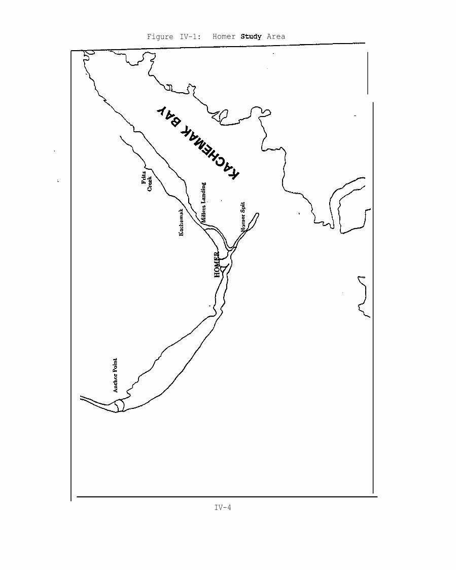
Figure IV-1: Homer Study Area

IV-4

We made additional assumptions to account for industries not

included in the Department of Labor data (e.g. fish harvesting) or

which were fully or partially suppressed (e.g. manufacturing and

wholesale trade) , and to allocate employment within a given

industry between resident and enclave shares? exogenous and

endogenous shares, etc. Our resulting employment assumptions for

the years 1980-1987 are shown in Table IV.2. Below we discuss

these assumptions by industry.

IV-5

Tab[e IV.1: Summary of Department of Labor En@oynant Data for Homer

Cateqorv Code 1980 1981 1982 1983 1984 1985 1986 1987

MiningConstructionManufacturingTrans., Comn., UtilitiesUhoLesale TradeRetai L TradeFin., Insm, & Real EstateServicesForestry, Ag., FisheriesFederaL GovernmentState GovernmentLocal Goverrw’mtTOTAL.

123456789101112

* * * * * * * *69 63 93 143 231 252 125 88140 * * * * * * *

IM 208 322 374 350 188 177 159* * 12 15 30 28 28 *

194 213 212 255 2!46 261 306 30340 46 52 60 74 74 68 57178 252 2.45 176 214 226 232 226

* * 11 * * * * *

31 32 36 36 “ 36 39 39 404 5 12 20 18 21 18 25

188 151 169 259 282 338 351 3471066 1499 1615 1747 1820 1727 1573 1466

* Data suppressed.

Iv-6

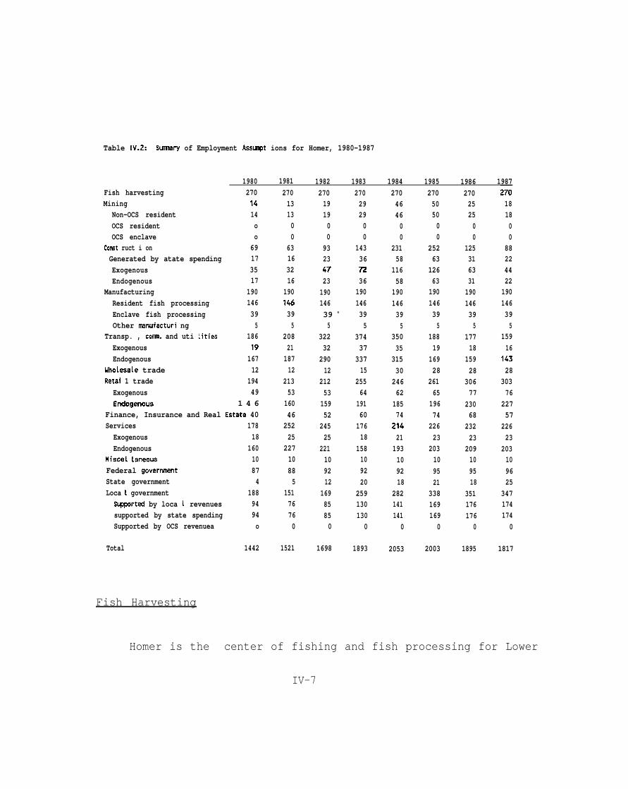
Table IV.2: Sumnary of Employment Assunpt ions for Homer, 1980-1987

1980 1981 1982 1983 1984 1985 1986 1987Fish harvesting 270Mining 14

Non-OCS resident 14OCS resident oOCS enclave o

Conat ruct i on 69Generated by atate spending 17Exogenous 35Endogenous 17

Manufacturing 190Resident fish processing 146Enclave fish processing 39Other menufacturi ng 5

Transp. , comn. and uti lities 186Exogenous 19Endogenous 167

Uholesale trade 12Retai 1 trade 194

Exogenous 49Endogenoua 1 4 6

Finance, Insurance and Real Estata 40Services 178

Exogenous 18Endogenous 160

MisceL laneoua 10Federal governnant 87State government 4Loca 1 government 188Sumrted by loca 1 revenues 94supported by state spending 94Supported by OCS revenuea o

Total 1442

Fish Harvesting

270131300

63163216

190146395

2082118712

213531604625225

22710885

15176760

1521

270191900

9323472319014639 e

53223229012

2125315952

24525

221109212

16985850

1698

270292900

143367236190146395

37437

33715

255641916017618

158109220

259130130

0

1893

270464600

23158

11658

190146395

35035

315302466218574

21421

193109218

282141141

0

2053

270505000

2526312663190146395

18819

16928

2616519674

22623

203109521

338169169

0

2003

270252500

125316331190146395

17718

15928

30677

23068

23223

209109518

351176176

0

1895

2%181800

88224422190146395

15916

14328

30376

22757

22623

203109625

347174174

0

1817

Homer is the center of fishing and fish processing for Lower

IV-7

Cook Inlet. Crab, bottomfish, and octopus fisheries operate

throughout the year. The seasonal fisheries begin with herring

and sablefish in April and March, then the various salmons (King,

Red, Pink, and Chum) from late

from October through December.

halibut landings in west coast

May through August, and Tanner Crab

Homer is second only to Kodiak in

Uese ports. In 1985, 353 people in

Homer held commercial fishing permits (Coughenower,

Alaska Department of Labor data was suppressed

agriculture, and fisheries” except during 1982 when

average was 11 employees (Table IV.1) . In 1980, TR

1987) .

for “forestry,

the annual

98 showed

resident fish harvesting at 429 FTE employment. However, for

comparison? Coughenower (1987] esti.imated 1~320 seasonal fishing

jobs in the Homer area and related these to 270 FTE jobs. He also

suggested an 83 percent resident share (i.e., 224 local FTE jobs) .

We have assumed resident fish harvesting employment of 270 for

1980-1987.

will remain

Mininq

We have also assumed that fish harvesting employment

constant at 270 for the period 1988-2020.

Non-OCS Resident. In 1980 TR 98 showed zero mining

employees. In 1985, Department of Labor showed three employers

with an average of 57 employees in the first quarter and three

Iv-8

employers with an average of 98 employees in the third quarter.

We are uncertain what this mining employment represents. It is

probably construction-related sand and gravel mining. Based on

the 1985 data, we assumed average annual mining employment of 50 in

1985. We assumed that mining employment between 1980 and 1987

varied in proportion to this assumed 1985 level. Subsequently,

for the period 1988-2020, we assumed that mining employment remains

constant at the 1987 level of 18.

.

OCS Mininq. We have assumed zero OCS mining employment in

the Homer area during the period 1980-1987. Similarly, our “base

case” model assumptions assumed zero OCS mining employment during

the period 1988-2020.

Loauinq

Kluk Waan is beginning timber harvests in the Ninilchik area

and plans to export the timber across the Homer dock. We assumed

that an average of 10 people were employed in logging between

1980-1987. We assumed that logging employment will remain

constant at 10 for 1988-2020.

IV-9

. .

Construction

According to Marnie Xsaacs with the Alaska Power Authority,

there was only limited employment during the period June 1986

through June 1987 on the Bradley Lake hydroelectric project.

During June 1987 through June 1988 there was no construction

because of need to clarify regulatory problems. Construction is

now continuing with a scheduled on-line date of September 1991.

The Alaska Department of Labor shows construction employment.

increasing from 69 in 1980 to 252 in 1985~ then dropping to 88

in 1987 (Table IV.1). (TR 98 showed construction l?TE employment

in 1980 at 132, nearly double the Department of Labor figure.)

We assumed that 25 percent of construction employment during

the period 1980-1987 was supported by state government capital

spending, 25 percent was exogenous, and 50 percent was endogenous,

based on our best judgment in the absence of any data.

According to the Alaska Power Authority, during the period

November 1988 through January 1989, an estimated 43 percent of

Bradley Lake employees were Homer area residents. Based on data

provided by the Power Authority, we assume that during 1988-1991

the average construction employment of Homer area residents on the

IV-1 O

Bradley Lake project will be 70. This brings estimated exogenous

construction employment to 114 during this period. We assumed the

1987 level

subsequent

absence of

of exogenous construction employment of 44 for the

period 1992-2020, based on our best judgment in the

any data.

Manufacturing

Total Manufacturing Em~loment. Fish processing is the 0

primary type of manufacturing in Homer. According to Coughenower

(1987), there were two major processors in the Homer area. One

had permanent facilities in Homer, the other in Seldovia. There -

are also processors who buy in the Homer area but are located

elsewhere as well as smaller specialty processors. Seward

Fisheries, part of Icicle Seafoods, is the largest processor

located in Homer.

Department of Labor showed manufacturing employment of

140 in 1980 (Table IV.1). For comparison, TR 98 showed fish

processing employment (FTE) in 1980 of 185 with 146 FTE’s resi-

dents and 38 FTE’s

Coughenower (1987)

employment of 105.

non-residents (.79 resident share) .

states that in 1985 Seward Fisheries had FTE

IV-11

.

We assumed that fish processing is constant at 185 (the 1980

level) with resident fish processing employment 147 and non-

resident employment 38. We assumed a 79 percent resident share for

fish processing employment during the years 1980-1987, which

resulted in an assumption of resident fish processing emplo~ent

of 146 and non-resident fish processing employment of 39 in 1987.

We assumed that both resident and non-resident fish

processing employment will remain constant at these assumed 1987

levels during the period 1988-2020..

Wood’Products . Two small lumber mills produce for local

building, one at Anchor Point the other on East End Road. We

assumed lumber mill employment of five for the period 1980-1987

and also for 1988-2020.

Transportation, Communications, and Utilities

Department of Labor average annual employment figures are

used. These range from 186 in 1980 to about 374 in 1983 then

decline to 159 in 1987 (Table IV.1). We assumed that 10 percent

of employment in this industry was exogenous and 90 percent was

endogenous. We assumed that exogenous transportation, communi-

cations and utilities employment will grow at 5 percent per year

IV-12

after 1987, based on an assumption that tourism in the Homer area

will grow at a rate of 5 percent per year.

Wholesale Trade

Department of Labor shows wholesale trade employment at

12 in 1982, increasing to 30 in 19841 thefi remaining steady at

28 in 1985 and 1986 (Table IV.1). We assumed that wholesale trade

employment was the same in 1980 and 1981 as in 1982 and also that

the 1987 figure was the same as in 1986 (Table IV.2). We assumed

that all wholesale trade employment was endogenous.

Retail Trade

Department of Labor annual average employment figures were

used for the retail trade category. These ranged from 194 in

1980 to 306 in 1986 and 303 in 1987 (Table IV.1). We assumed that

25 percent of retail trade employment was exogenous and 75 percent

was endogenous. We assumed that exogenous retail trade employment

will grow at a rate of 5 percent per year after 1987.

Finance, Insurance, and Real Estate

.

Department of Labor annual average employment figures were

Iv- 13

used for this category. “FIRE” employment increased from 40

employees in 1980 to 74 in 1984 and 1985 then decreased to 57 in

1987 (Table 3X7.1). We assumed that all employment in these

industries was endogenous.

Services

We used Department of Labor annual average employment figures

for this category (Table IV.1). Services employment increased

from 178 in 1980 to 252 in 1981 and then declined to 176 in 1983

but then increased to 232 in 1986 (Table XV.1). In 1987 services

employment had dropped’ off slightly to 226. We assumed that 10

percent of employment in this industry was exogenous and 90

percent was endogenous. Based on information provided by the

Power Authority, we assumed that Bradley Lake construction will

add 20 employees to the Homer area services sector during 1988-

1991. After 1991 we assume that services employment will drop

back to the 1987 level. We assumed that exogenous services

employment (with the exception of Bradley-Lake-generated

employment) will grow at a rate of 5 percent per year after 1987.

Federal Government

Civilian federal government employment in Homer increased

IV-14

from 31 in 1980 to 40 in 1987 (Table IV.1). The Coast Guard

maintains one unit in Homer with 56 personnel. We project federal

government employment at 96 for 1988-2020.

State Government

State employment increased from 4 in 1980 to 25 in 1987

(Table IV.1). We assume that state government employment is

endogenous.

Local Government

Department of Labor annual averages show 188 local government

employees in 1980, increasing to 351 employees in 1986 and 347 in

1987 (Table IV.1). We assumed that 50 percent of this employment

is funded by local revenues and the rest by state revenue sharing.

IV- 15

Table IV.3: Estimated Employment in Homer

1980 1981 1982 1983 1984 1985 1986 1987

Resident BasicFishingFish ProcessingHi scet 1 aneousother (mining, manufacturing)

Resident SupportExogenousEdogenousGovermnent SponsoredEnclave Sponsorad

Resident GovernmentExogenousEndogenous

Total ResidentTotal ExogenousTotat Endogenous

4452701461019

67911954217

27987192

14036!51732

Non-Resident <Enclave) Employment 39

Total Resident and Non-Resident 1442

4442701461018

79413!64816

24488

156

1482663819

39

1521

4502701461024

93615675723

27392

{81

1659

961

39

1698

4602701461034

102319079736

37192279

18547421112

39

1893

4772701461051

11452%385458

39292

300

20148031212

39

2053

4822701461055

102923373363

45495

359

19658091155

39

2003

4562701461030

95618072531

46495

369

1856731

1125

39

1895

4492701461023

861! 5868122

46896

372

1778703

1075

39

1817

Emnlovment Multipliers

Table IV.3 summarizes employment “multipliers” for the period

1980-1987. In general, these multipliers remain relatively

constant throughout the period. This suggests thati the economic

structure of Homer was relatively stable during this period.

I V - 1 6

,,

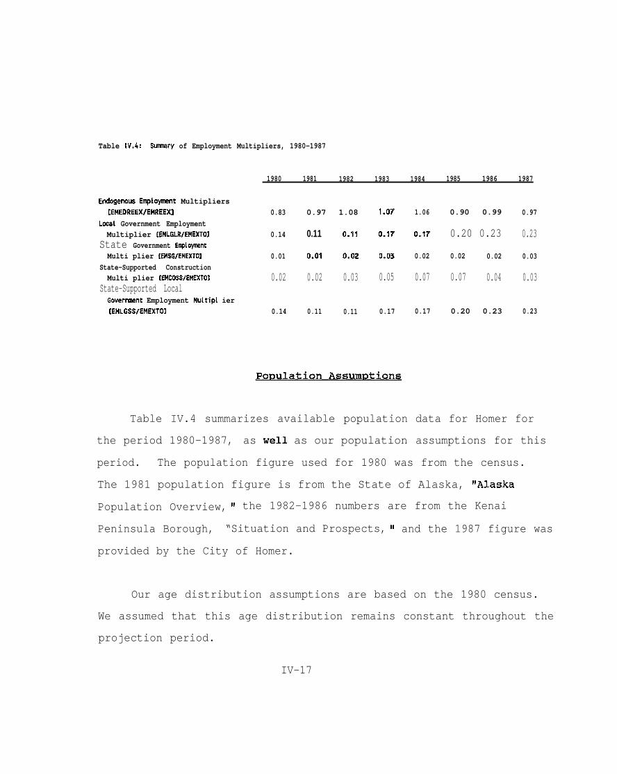
Table lV.4: Sunnary of Employment Multipliers, 1980-1987

1980 1981 1982 1983 1984 1985 1986 1987

Endogenous Empioynant Multipliers[EMEOREEX/EMREEXl 0.83 0.97 1.08 1.07 1.06 0.90 0.99 0.97

LoCat Government EmploymentMultiplier [EMLGLR/EMEXTOl 0.14 0.11 0.71 0.17 0.17’ 0.20 0.23 0.23

State Government E~LoymantMulti plier [EMSG/EMEXTOl 0.01 0.01 0.02 0.03 0.02 0.02 0.02 0.03

State-Supported ConstructionMulti plier [EMCOSS/EMEXTOl 0.02 0.02 0.03 0.05 0.07 0.07 0.04 0.03

State-Supported LocalGoverrunent Employment Multipt ier[EMLGSS/EMEXTOl 0.14 0.11 0.11 0.17 0.17 0.20 0.23 0.23

Powlation Assum~tions

Table IV.4 summarizes available population

the period 1980-1987, as well as our population

data for Homer for

assumptions for this

period. The population figure used for 1980 was from the census.

The 1981 population figure is from the State of Alaska, ItAlaska

Population Overview, 11 the 1982-1986 numbers are from the Kenai

Peninsula Borough, “Situation and Prospects, “ and the 1987 figure was

provided by the City of Homer.

Our age distribution assumptions are based on the 1980 census.

We assumed that this age distribution remains constant throughout the

projection period.

IV-17

The ratio of assumed resident population to assumed resident

exogenous employment increased from 3.33 in 1980 to 5.66 in 1987.

The fact that this ratio increased steadily suggests that, either our

employment figures or our population data (or both) may be

unreliable. However, in”the absence of better data we nevertheless

assumed that in the future this ratio remains constant at the 1987

level.

.

IV-18

,..

Table IV.4: Population Data for Homer, 1980-1987

1980 1981 1982 1983 1984 1985 19% 1987

Peculation Data

1980 Census 2209

by age groupo-4 1995-19 54420-64 136265+ 104

Homer (Alaska Population Overvi W)l5

2588 2900 3114 3373Homer (Situation and Prospects) 2897 3237 3429 3817 4020Homer (City of Homer) 4020

Permanant Fund DividendDistributions 5906 6067 6341 6936

Adult 4044 4169 4339 4745Chi ldran 1862 1898 2002 2191

School Enrollment 1029 993 1063 1149 1120 1120

Pomlation Assunmt iona

Resident Population: TotaL 2209 2461 2858 3198 3390 3778 3981 3981Age Distribution (percent)

Pre-School (O-4) 0.09School-age (5-19) 0.25Adult (20-64) 0.62Senior (65+) 0.05

Resident Exogenous Employment 651 663 698 742 803 809 731 703Ratio of Resident Population toResident Exogenous Employment 3.33 3.85 4.10 4.31 4.22 4.67 5.45 5.66

1 llA1aska po~lation Overview, ii September 1985.2 IIsituation ati prospecta,ll Kenai Peninsula Borough, 1985, 1986, 1987

IV-19

Base Case Projections

Figure IV.2 and Table IV.6 summarize our base case projections

for Homer. Total population rises gradually over the projection

period. This is due primarily to increasing tourism.

.

IV-2 O

7

1

c1

Figure IV-2: Homer Base Case Projections

BASE CASE EMPLCIYMENT AND POPUIAT’KIN

;

Total PQP

I en Population

/~Tctal Emcbmwsldent Employment

A@

Enclave Employment & Population

1980- 1985 1990 1995 2mo 2005 201 Q 2015 2020

‘fE4R

IV-2 1

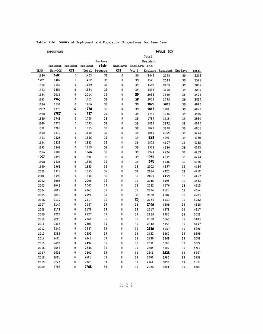
Table IV.6: Sumnary of Employment and Population Projections for Baae Case

EMPLOYMENT POPULAT IONTotal,

Enclave ResidentResident Resident Resident Fish- Enclave Enclave and

YEAR Non-OCS Ocs Total Process. Ocs T’ota 1 Enclave Resident Enclave Total19801981198219831984198519861987198819891990199119921993199419951996199719981999200020012002200320042005200620072008200920102011201220132014201520162017201820192020

14031482165918542014?96518561778175717481773178518101826183318691886189119361963197519902006204320652091211721472178222722612303234723932441249225462602266127232788

00000000000000000000000000000000000000000

140314821659185420141965185617781757174817731785181018261833186918861891193619631975199020062043206520912117214721782227226123032347239324412492254626022661272327/3S

3939393939393939393939393939393939393939393939393939393939393939393939393939393939

00000000000000000000000000000000000000000

3939393939393939393939393939393939393939393939393939393939393939393939393939393939

14421521169818932053200318%1817’17961787181218231849186518721908192419501974200220142029204520822104213021562786221722662300234223&524322480253125852641270027612826

2170254928583198339037783981398139363915397239984055409141074186422442354336439744234459449445764625468447434809487849905065515852575360546955835702

596060996244

3939393939393939393939393939393939393939393939393939393939393939393939393939393939

22092588289732373429381740204020397539544010403640944130414542254263427443754436446244974533461546644723478248484917502851035197529653995508562257415867599961376283

IV-2 2

References

Alaska Department of Labor, Alaska Population Overview 1985Estimates, April 1987.

Alaska Department of Labor, Employment Database Files forCordova, Homer, Kenai, Kodiak, Seward, and Yakutat, November1988 (unpublished).

Alaska Department of Labor, Geocmanhical Area ClassificationManual. January 1981.

Alaska Department of Labor, July 1 Population Estimates, NewsRelease, March 1, 1988.

Alaska Department of Revenue, Permanent Fund Dividend ReciDientProfiles.

Alaska Power Authority, F.E.R.C. Armlication for License for MajorUnconstructed Proiect, Bradlev Lake Hydroelectric Proiect,Bradlev River. Kenai Peninsula. Alaska, Volume 3, Exhibit E,Chapter 5, Report on Socioeconomic Impacts (received byFederal Resources Library, Anchorage, Alaska August 1,1988) .

Bechtol, Eileen R. City of Homer, Telephone Interview. October 28,1988.

Coughenower, D. Douglas, Commercial Fishina Industrv Studv Homer.Alaska, University of Alaska, Marine Advisory Program,Marine Advisory Bulletin #33, November 1987.

Dames and Moore, Homer Spit Coastal Develo~ment Promam,Identification of Homer SDit Coastal Development Needs,prepared for Kenai Peninsula Borough, City of Homer, andAlaska Coastal Management Program, 1981.

Fried, Neal, “Employment in Alaska’s Seafood Industry,” AlaskaEconomic Trends, Juneau, Alaska: Alaska Department of Labor,July 1987.

Homer, City of, “Preparing for Tomorrow Today, “ InformationalBrochure.

Kenai Peninsula Borough, Situation and Prospects, 1985,1986, 1987, 1988.

Keiser, Gretchen, and Pierce, Brad. State of Alaska Budaet, FY 84-

S?-23

FY 87. Alaska State Legislature, House Research AgencyReport 87-C, February 1987.

Knapp, Gunnar; Nebesky, W.; Hull, T.; White, K.; Reeder, B.; andZimicki, J. Gulf of Alaska Economic and Demoara~hic SystemsAnalvsis. University of Alaska, Institute of Social andEconomic Research, ‘(Prepared for Minerals and ManagementService, Alaska OCS Office) Social and Economic StudiesProgram, Technical Report Number 98, March 1984.

Livey, Jay, and Keiser, Gretchen. Public School Financincr inAlaska. Alaska State Legislature, House Research AgencyReport 87-A, February 1987.

Pacific Rim Planners and Engineers a Division of OlympicAssociates Company, Citv of Homer. Com~rehensive Plan, 1983.

U.S. Census, 1980.

IV-2 4

CHAPTER V. DESCRIPTION AND MODEL ASSUMPTIONS: KENAI MARKET AREA

Overview

Kenai is located south of Anchorage, across Turnagain Arm,

and on the northwestern part of the Kenai Peninsula. The Kenai

study area (market area) encompasses the northwestern part of the

central Kenai Peninsula

Soldotna as well as the

Sterling, and Kasilof.

and includes the communities of Kenai and

areas of Nikishka, Salamatof, Kalifonski,

This area is approximately 160 miles south

of Anchorage via the Seward and Sterling Highways. It has

airports at Soldotna and Kenai and there are deep water loading

facilities for the petroleum products at Nikiski.

Kenai, with a population of about 6,550, is dominated by the

oil/natural gas industry. Tourists and sports fishermen contri-

bute to the economy during the summer months, attracted by salmon

fishing on the Kenai River, clam tides on Cook Inlet, and other

the opportunity to partake in other outdoor activities. Commer-

cial fishing and fish processing also contribute to the economy.

The Kenai National Moose Range is also an attraction as are other

state recreation

round employment

facilities. Government provides stable year-

opportunities since this area is the regional

v-l

center for

Total

the Borough government.

employment in the Kenai Market Area increased between

1980 and 2987. The strongest growth sectors were retail trade,

services and government. However, employment in other sectors

decreased during this period:

transportation, communications

mining; construction; and

and utilities.

Maior’ Data Sources

The primary data source for our analysis of Kenai was

Department of Labor data on employment for Kenai and the ‘lKenai

market area.’~ In addition we used the Kenai Peninsula Borough

publication F!Situation and. Prospects” for 1985, 1986, 1987, and

1988; the Alaska Department of Labor ‘Population OverviewJt publi-

cations; and “Gulf of Alaska Economic and Demographic Systems

Analysis,” Social and Economic Studies Program, Technical Report

Number 98, March 1984 (subsequently referred to as TR 98). We

also discussed the outlook for Cook Inlet oil and gas production

with Department of Revenue Petroleum Economist, Dr. Charles

Logsdon.

We have listed all of the sources used in our analysis at the

end of this chapter.

v - 2

Study Area

Figure V.1 shows the area which we are defining as the

ilKenai market area. “ Our employment and population assumptions

and projections for this study refer to employment and population

within this area. We combined Department of Labor sub-sub areas

712 (Kenai City) and 713 (Soldotna) to reflect the Kenai Market

Area. The sub-sub area 713 includes the following localities:

Bernice Lake, Clam Gulch, Cohoe, Drift River, Kalifonsky, Kasilof,

Nikishka,

Sterling,

Point Possession, Salamatof, Skilak Lake, Soldotna,

Swanson, Tustumena, and Wildwood.

Em~lovment Assum~tions

Table V.1 shows Alaska Department of Labor employment data

for the Kenai Market Area for the years 1980-1987. These data

formed the primary basis for the development of our employment

assumptions, and are the basis for all employment data not

otherwise cited.

We made additional assumptions

included in the Department of Labor

to account for industries not

data (e.g. fish harvesting) or

v - 3

Figure V-1: Kenai Study Area

- KenaiCity

%Idontaaty *

N

A

w- -E

s

\

V-.4

which were fully or partially suppressed (e.g. manufacturing and

wholesale trade) , and to allocate employment within a given

industry between resident and enclave shares, exogenous and

endogenous shares, etc. Our resulting employment assumptions for

the years 1980-1987 are shown in Table V.2. Below we discuss

these assumptions by industry.

. v-5

Table V. 1: Sunnary of Department of Labor Emptoymant Data for the Kanai Market Areal

Cateqorv Code 1980 1981 1982 1983 1984 1985 1986 1987

MiningConstruct ionManufacturingTrans., Ccmn., UtilitiesUholesate TradeRetai L TradeFin., Ins., & Real EstateServi ceaForestry, Ag., FisheriesFederal GoverrmantState GovernmentLocal GovernmentTOTAL

1 m 718 1038i? 514 608 6733 1024 856 9244 521 582 6325 236 310 2786 675 706 8007 * 177 2068 642 708 7739 * * *

10 76 74 7711 323 365 40412 754 804 891

5635 6006 6524

; Data Suppressad.Data are suns of totals for sub-sub areas 712 and 71.3.

558790922634289973

*

%1*

92456961

6209778915893411275

*

1086*

10052410537789

725102910686023241498

*

118’5*

10856111348580

85061910124003071556

*

1257*

105571

10427990

6884211042354291

1331*

1260*

107545

11307483

V-6

Table V.2: Sh.mnary

Fish harvestingUining

Non-OCS residentNon-OCS enclaveocs residentOCS enclave

Construct ion

of Employment Assmpt ions for Kenai Market Area, 1980-1987

Generatad by state spendingExogenousEndogenous

ManufacturingResident fish processingEnclave fish processingOther manufacture ng

Transp., coinn., and utititiesExogenousEndogenous

Wholesale tradeRetai 1 trade

ExogenousEndogenous

Finance, Insurance and Real EstateServices

ExogenousEndogenous

Hi scel (aneousLogging

Federal governmentState govermiantLoca L goverrunent

Supported by local revenuesSupported by state spandingSupported by OCS revenues

Total

1980 1981 1982 1983 1984 1985 1986 1987

159733367367

00

514129129257

102422233446852152

469236675169506! 63642&i

57800

813237%3773n

159718359359

00

60815215230485615523346858258

52431070617753017770871

63700

79365804402402

159634317317

00

673168168337924182274468

63569278800200600206m77

69600

82404891446446

159558279279

00

79019819839592218227246863463

57128997324373022596196

86500

97456961481481

0 0 0 0

159620310310

00

97724424448989116925446858959

5303411275319956252

1086109977

00

1055241053527527

0

159725363363

00

1029257257515

106822433650860260

54232414983751124279

1185119

106700

113561

1134567567

0

159850425425

00

619155155310101220230250840040

36030713563391017265

1257126

113100

110571

1042521521

0

159688344344

00

421105105211

104221432050835435

319291

1331333998203

1260126

113400

112545

1130565565~

5825 6072 6456 7025 7872 8677 7948 7536

v - 7

Fish Harvesting

Full-time equivalent. employment in fish harvesting was 159 in

1980 (TR 98). Although this may understate full-time fish

harvesting employment in more recent years, we have assumed this

figure for the period 1980-1987. We have also assumed that fish

harvesting employment will remain constant at this level for the

period 1988-2020.

Mininq

Non-OCS Resident. The largest employer on the Central Kenai

Peninsula is the oil and gas industry with the greatest concen-

tration of development in the North Kenai area. The following

description of the oil and gas industry is given in TR 98:

Since the late 1950’s, the oil and gas industry has been the

major economic activity in the Kenai area. Producing oil and

gas fields at Swanson River and in Upper Cook Inlet marked a

major phase in Alaska’s petroleum development. In the

1960’s, four oil fields and fourteen gas fields in Upper Cook

Inlet were developed. Oil production peaked in 1970. Proven

natural gas reserves are predicted to last beyond the year

V-8

2000 under existing usage patterns. Extensive processing

plants and pipeline facilities were built in the 1960’s and

1970’s. They are located at Nikiski, north of the city of

Kenai, and consist of two refineries~ an ammonia-urea plant,

a liquified natural gas plant, and crude oil storage and

loading facilities.

The mining

field workers.

category includes mostly ~ook Inlet gas and oil

According to Department of Labor, average annual

employment increased from 733 in 1980 to a high of 850 in 1986

then declined to 688 in 1987 (Table V.2). Charles Logsdon,

Department of Revenue, said that it is typically assumed that 50

percent of the platform employees will be residents and 50 percent

will be enclave (i.e., commute to homes elsewhere) . This

relationship is maintained in the model.

Although the Kenai gas fields are nearly depleted, there are

new fields coming on-line that should offset production decline

from the old fields. We discussed the future of Cook Inlet oil

and gas production with Dr. Logsdon. He expects thati Cook Inlet

oil fields will continue producing 15,000 to 20,000 barrels per

day for quite a few more years. According to Logsdon, new produc-

tion developments will in all likelihood continue to offset

natural field decline and thus result in relatively stable produc-

V - 9

tion and processing levels over time, barring no significant new

developments. Therefore, we assume that mining (production) and

oil and gas processing employment will remain constant at the 1987

levels through 2020 and tha% there will be no new developments

such as a gas pipeline from the North Slope; another .Liquified

Natural Gas (LNG) facility producing for export; a major Beluga

Coal extraction project; or

We assume that non-OCS

incremental gas processing facilities.

resident and enclave employment is

split half and half during 1980-1987. From 1988 to 2020 we assume

that

each

total non-OCS mining and oil and gas employment is 688 in

year with 344 enclave and 344 resident employees.

OCS Mining. We have assumed zero OCS mining employment in

the Kenai Market Area during the period 1980-1987. Similarly, our

“base case” model assumptions assume zero OCS mining employment

during the period 1988-2020.

Construction

The Alaska Department of Labor shows annual average

construction employment of 514 in 1980, increasing to 1,029 in

1985, then declining to 619 in 1986 and 421 in 1987 (Table V.I).

v - l o

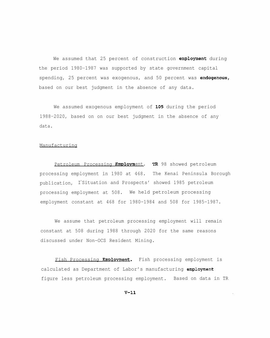
We assumed that 25 percent of construction emplonent during

the period 1980-1987 was supported by state government capital

spending, 25 percent was exogenous, and 50 percent was endogenous,

based on our best judgment in the absence of any data.

We assumed exogenous employment of 105 during the period

1988-2020, based on on our best judgment in the absence of any

data.

Manufacturing

Petroleum Processing Em~lovment. TR 98 showed petroleum

processing employment in 1980 at 468. The Kenai Peninsula Borough

publication, ItSituation and Prospects’ showed 1985 petroleum

processing employment at 508. We held petroleum processing

employment constant at 468 for 1980-1984 and 508 for 1985-1987.

We assume that petroleum processing employment will remain

constant at 508 during 1988 through 2020 for the same reasons

discussed under Non-OCS Resident Mining.

Fish Processing Em~lovment. Fish processing employment is

calculated as Department of Labor’s manufacturing emplo~ent

figure less petroleum processing employment. Based on data in TR

98, it is assumed that resident fish processing employment is .4o

and non-resident is .6. We assumed a 40 percent resident share

for fish processing employment during the years 1980-1987. Resident

fish processing employment is thus 214 and non-resident fish

processing employment 320 in 1987.

We assumed that both resident and non-resident fish

processing employment will remain constant at their 1987 levels

during the period 1988-2020.

Transportation, Communications. and Utilities

Department of Labor average annual employment figures are

used. These ranged from 521 in 1980 to 634 in 1983 then declined

to 354 in 1987 (Table V.I). We assumed that 10 percent of

employment in this industry was exogenous and 90 percent was

endogenous. We assumed that exogenous transportation, communi-

cations and utilities employment will grow at 3 percent per year

after 1987, based on an assumption that economic activity related

to tourism in the Kenai Market Area will continue to expand.

Wholesale Trade

Department of Labor averages show employment of 236 in 1980,

V-12

increasing to 341 in 1984 then decreasing to 291 in 1987 (Table

V*1) . We assumed that all wholesale trade employment was

endogenous.

Retail Trade

Average annual employment in retail trade increased from 675

in 1980 to 1,498 in 1985 then decreased to 1,331 in 1987 (Table

V.1) . This large increase probably reflects some rapid growth in

the seasonal tourist/sports-fishing industry as well as the

economic expansion experienced in Alaska during this period. We

assumed that 25 percent of retail trade employment was exogenous

and 75 percent was endogenous. We assumed that exogenous retail

trade employment will grow at a rate of 3 percent per year after

1987.

Finance, Insurance, and Real Estate

Extrapolating from Department of Labor data available for

1981 and 1982 and based on service sector employment trends in

the Kenai Market Area, we assume that annual average employment in

finance, insurance and real estate increased from 163 in 1980 to

an

We

estimated 279 in 1985 then declined to 203 in 1987 (Table V.1).

assumed that all employment in these industries was endogenous.

V-13

.-

Services

Average annual employment in services increased from 642 in

1980 to 1,260 in 1987 (Table V.1). We assumed that 10 percent of

employment in this industry was exogenous and 90 percent was

endogenous. We assumed that exogenous services employment will

grow at a rate of 3 percent per year after 1987.

Federal Government

Civilian federal government employment increased from 76 in

1980 to 107 in 1987. The U.S. Coasti Guard stations !5 personnel ah

Kenai. Table V.2 reflects total federal employment (civilian and

military) . We assume

and project it at the

State Government

State government

1980 to a high of 571

V.1) . We assume that

that federal employment is totally exogenous

1987 level of 112 for 1988-2020.

employment increased from 323 in

in 1986 then declined to 545 in 1987 (Table

state government employment is endogenous.

V - 1 4

Local Government

Local government employment increased from 754 in 1980 to

1,134 in 1985 then declined to 1,130 in 1987 (Table V.1). Local

government employment includes components lisupported by state

spending” and “supported by local revenues” which we assume to be

endogenous. It also includes “local government supported by OCS

revenues.” This category is exogenous and we assume that it is

zero for 1988-2020.

V-15

Table V.3: Estimated EnqaLoyment in the Kenei Market Area

Resident BasicFishingFish ProcessingHi sceL LaneousMining & OiL & GasPetroLetm Proc. & Other !lfg.

Resident SuwrtExogenousEndogenousGoverrmient SponsoredEnclave Sponsored

Resident GovernmentExogenousEndogenous

Totel ResidentTotaL ExogenousTotaL Endogenous

Non-Resident (Enclave) En@oyment

TotaL Resident PLUS Non-Resident

Emnlovment Multipliers

1980 1981 1982 1983 1984 1985 1986 1987

748159222

0367468

275?4142209129

115881

1077

512517103414

700

5825

673159155

0359468

3091458

2482152

124879

1169

548016783803

592

6072

658159182

0317468

5092685168

137782

1295

171741G

591

6456

620159182

0279468

38?2600

3074198

151497

1417

647417854689

551

7025

638159169

0310468

4520731

3545244

1682105

1577

730819425367

56&

7872

Table V.4 summarizes employment “multipliers”

746159224

0363508

4917810

3849257

1808113

1695

797921775802

699

8677

786159202

0425508

4204659

3390155

1723110

1613

722120635158

727

7948

for the

717159214

0344508

3860599

3155105

1787112

1675

687219364936

664

7536

period 1980-1987. In general, the government multipliers (local

government employment, state government employment, and state-

supported local government employment) increased during this

period. The state-supported construction and endogenous employ-

V-16

ment multipliers increased during 1980-1984 then declined through

1987. We believe that these relations adequately reflect the

economic changes that occurred during this period.

Table V.4: sumary of Employment Multipliers, Kanai Market Area, 1980-1987

1980 1981 1982 1983 1984 1985 1986 1987

Endogenous En@oymant Multipliers[EMEDREEX/EMREEXl

Loca 1 Governmnt EnploymsntMulti plier [EMLGLR/EMEXTOl

Stete Government EnqaloymentMulti plier [EMSG/E14EXTOI

Stste-Supported ConstructionMulti PL i er [EMCOSS/EMEXTOl

State-Supported LocalGovernment Employment Multiplier[EMLGSS/EMEXTOl

1.26 1.46 1.55 1.71 1.81 1.75 1.63 1.61

0.16 0.18 0.19 0.21 0.21 0.20 0.19 0.22

0.13 0.16 0.18 0.20 0.21 0.20 0.20 0.21

0.05 0.07 0.07 0.08 0.10 0.09 0.06 0.04

0.16 0.18 0.19 0.21 0.21 0.20 0.19 0.22

Po?3ulation Assumptions

Table V.5 summarizes available population data for Kenai for

the period 1980-1987, as well as our population assumptions for this

period. Our 1980 assumption for total population was based on the

1980 census. Our assumptions for 1981, 1982 and 1985-1987 are based

on Kenai Peninsula Borough figures; 1983 and 1984 are based on State

of Alaska figures. We extrapolated population for the Kenai Market

Area in 1981 and 1985 because population figures were not available

V-17

for the smaller areas within the Kenai Market Area.

Our age distribution assumptions are based cm the 1!380 census.

We assume that this age distribution remains constant throughout the

projection period.

The ratio of assumed resident population to assumed resident

exogenous employment increased dramatically from 5.03 in 1980 to

12.93 in 1987. The fact that this ratio more than doubled suggests

that either our employment figures or our population data (or both)

may be unreliable, or our assumption is not justified that these two

figures are closely correlated. However, in the absence of better

data we nevertheless assume that in the future this ratio remains

constant at the 1987 level.

V-18

Table V.5: Po~lation Data for Kenai Market Area, 1980-1987

1980 1981 1982 1983 1984 1985 1986 1987Population Data

1980 Censusby age group

o-45-1920-6465+

Kenai Market Area PopulationKena iSo 1 dotnaNikishkaSalamatofSterlingKasi lofKal i f onski

Tota(

Permanent Fund DividendDistributions

AdultChildren

School Enrollment

Pomlation Assmot ionaResident Population: TotatAge Distribution (percent)

Pre-School (O-4)School-age (5-19)Adult (20-64)Senior (65+)

Resident Exogenous EmploymentRatio of Resident Population toResident Exogenous Employment

9299

89226265593188

43242320110933491920192

9299

4558 52312445 3008

29771143183720712564

16300 18831

572133539196511328491258

12721

6173359710096941530567

2 9 5

13865

6434 65463597 3648

41691394280037144002

24820 25693

20182 20905 22787 25181

6546366841691394280031194006

25702

2925 4079 4463 4655 5281 5485 5499 5325

8599 15708 18240 12170 13301 24122 24966 25038

0.100.280.600.02

1710 1678 1717 1785 1942 2177 2063 1936

5.03 9.36 10.62 6.82 6.85 11.08 12.10 12.93

V-19

Base Case Projections

Figure V-2 and Table V.6 summarize our base case projections for

Kenai. Total population rises gradually over the projection period.

This is due primarily to increasing tourism.

I

30 128 i

26 --(24~.,.- 1

Fi~re V-2: Kenai Base Case Projections

:(: E ~],~1

8ASE CASE EMPLOYMENT AND POPULATION32 ,

Total POP

-

r~

. Pqwdon

,-

4

?.

+ IEndow Employment & Popuiatlon

t

I

7980 19a5 1990 199s 2 m o 2006 2010 2015 2020

‘fE4R

.V-21

Table v.6: Smnary of En@oymant end Population Projectionsfor Base Case

EMPLOYMENT POPULATIONTotal,

Enc L ave ResidentResident Resident Resident Non- Enclave Enclave and

YEAR Uon-OCS Ocs Total Ocs Ocs Tota 1 Enclave Resident Enclave Tota i19801981198219831984198519861987198819891990199119921993199419951996199719981999200020012002200320042005200620072008200920102011201220132014201520162017201820192020

5125548058656474730879797221687268406759

699170377029717572147187737274577453746774777592762576757719777678317977803481258219831684168519

8734884789629082

00000000000000000000000000000000000000000

5125548058656474730879797221687268406759*268896991703770297175721471877372745774’5374677477759276257675771977767831797780348125821983168416851986258734884789629082

700592591551564699727&$665665665665665665665665665665665665665665665665665665665665665665665665665665665665665665665665665

00000000000000000000000000000000000000000

700592591551564699727664665665665665665665&556656656656656656636656656656656656656656656656656656&5665665665645665665665665

5825607264567025787286777948753675057424752773547656

769478407879785280378122817881328142825782908340838484418496864286998790888489819081918492909399951296279747

8599157081824012!70133012412224966

246222433224702248002516625334253042583025972258722653826846268312688026917273322744827629277892799228192287182892129250295892993830298306683105037443318473226432694

700592591551564699727664665665665665665665665665665665665665665665fM5665665665665665665665665665665665665665665665665665665

929916300188311272113865248202569325702252872499725367254652583125999259692649526637265372720327511274962754527582279972811328294284542865728857293832958629W5302543060330963313333171532108325123292933359

v-22

References

Alaska Department of Labor, Alaska Po?mlation Overview 1985Estimates, April 1987.

Alaska Department of Labor, Employment Database Files forCordova, Homer, Kenai, Kodiak, Seward, and Yakutat, November1988 (unpublished).

Alaska Department of Labor, Geoura~hical Area ClassificationManual. January 1981.

Alaska Department of Labor, July 1 Population Estimates, NewsRelease, March 1, 1988.

Alaska Department of Revenue, Permanent Fund Dividend RecipientProfiles.

Kenai Peninsula Borough, Situation and Pros~ects, 1985,1986, 1987, 1988.

Keiser, Gretchen, and Pierce, Brad. State of Alaska Budqet, FY 84-FY 87. Alaska State Legislature, House Research AgencyReport 87-C, February 1987.

Knapp, Gunnar; Nebesky, W.; Hull, T.; White, K.; Reeder, B.; andZimicki, J. Gulf of Alaska Economic and DemoaraDhic SystemsAnalvsis. University of Alaska, Institute of Social andEconomic Research, (Prepared for Minerals and ManagementService, Alaska OCS Office) Social and Economic StudiesProgram, Technical Report Number 98, March 1984.

Livey, Jay, and Keiser, Gretchen. Public School Financincl inAlaska. Alaska State Legislature, House Research AgencyReport 87-A, February 1987.

Logsdon, Charles L. Alaska Department of Revenue, Oil and GasAudit Division. Personal Communication. December 28, 1988.

U.S. Census, 1980.

V-23

CHAPTER VI. DESCRIPTION AND MODEL ASSUMPTIONS: KODIAK

Overview

The Kodiak study area encompasses the Kodiak Island Borough.

The highest concentration of people is in the road connected area,

however, data is most generally available for the entire borough.

Kodiak Island is a mountainous, rugged area with a fjord-type

coastline. The northern part of the island is timbered with

coniferous forests of northern spruces, this vegetation

transitions to deciduous cottonwoods, alders, and birch type

forests to the south, with the far southernmost part of the

island very open and windswept with virtually no vegetation other

than hardy grasses. Communities are generally located at sites of

bays and harbors protected from the harsh seas of the Gulf of

Alaska. Kodiak is the largest community in the borough with over

half of the borough population. The other communities, such as

Old Harbor, Larson Bay, Ouzinkie, Akhiok, tend to have fishing and

subsistence based economies.

Kodiak Island, located south of the Kenai Peninsula, is

approximately 45 minutes from Anchorage by air. Kodiak has air

VI-1

service by commuter planes as well as jets. It can also be

reached from the Kenai Peninsula on the Alaska Marine Highway

System.

Kodiak is the center for fishing activities for the Gulf of

Alaska, south of the Kenai Peninsula and east of the Aleutian

Chain. Tourism and sports hunting/fishing is supported. An

estimated 25 percent of Kodiak employment was generated by outdoor

recreation activities and non-resident tourism. There is also a

Coast Guard base and a small amount of ranching/agriculture.

Borough government offices are located in Kodiak.

During the 1980’s major construction projects dn Kodiak

Island included the Terror Lake Hydroelectric Project, the Near

Island Bridge, the Dog Bay Boat Harbor, and sewer and water

expansion.

Total Kodiak employment decreased during the 1980’s. Manu-

facturing; transportation, communications, and utilities; and

federal government employment declined. The other sectors were

either relatively stable or increased slightly.

VT-2

Maior Data Sources

The primary data source for our analysis of Kodiak was

Department of Labor data on employment for Kodiak. In addition we

used Alaska Department of Labor “Population Oveniew” publica-

tions, l~The Center of Alaska’s Bottomfish Grounds: Kodiak and the

Aleutian Islands” and “Employment in Alaska’s Seafood Industry”

by Neil Fried, published in Alaska Economic Trends (July 1988 and

July 1987, respectively) , and IiTechnical Report Number 122: A

Description of the Economic and Social Systems of the Kodiak-

Shumagin Region,” U.S. Department of the Interior (1986).

We have listed all of the sources used in our analysis at the end

of this chapter.

Study Area

Our employment and population assumptions and projections for

the study refer to employment and population within the road-con-

nected area around the City of Kodiak, including the Coast Guard

base (Figure VI.1). Although the sub-sub area (741) that we used

for employment statistics was the “Kodiak City SSA,” we added in

‘estimates of Coast Guard personnel. Based on historical relation-

ships, we adjusted the borough population downward by 10 percent

VI-3

to reflect an estimated population within the road-connected

EmDlovment Assumptions

area.

Table VX.I shows Alaska Department of Labor employment data

for the years 1980-1987. These data formed the primary basis for

the development of our employment assumptions, and are the basis

for all employment data not otherwise cited.

We made additional assumptions to account for industries not

included in the Department of Labor data (e.g. fish harvesting) or

which were fully or partially suppressed (e.g. manufacturing and

wholesale trade) * and to allocate employment within a given

industry between resident and enclave sharesr exogenous and

endogenous shares, etc. Our resulting employment assumptions for

the years 1980-1987 are shown in Table VT.2. Below we discuss

these assumptions by industry.

VI-4

Figure VI-1: Kodiak Study Area

.—. -?-,/”-’%U&& :

-,/:

;

,# -- -’~’. ----- - - - z

E,*,- r=

-- I .I cc-

-ix/ . . . -

“::%(

-.

“’:’---::%~-- \@ —nct. -

‘+’ -.-;. . . J -, ’; L<f”

,,2, F (’ . . . . . /“”

- i“Wnim mm yg

- -/

slopFIIk

S.**----

-.%.,O -*:.

.. ..

. .

//Tw?Uks I

. .

VI -5

Table VI.1: Sumnary of Department of Labor Employment Data for Kodiak City SSA

Cate90ry Code 1980 1981 1982 1983 1984 1985 1986 1987

MiningConstruct ionManufacturingTrans., Coimn., UtiWhoLesaLe TradeRetail TradeFin., Ins., & RealServices

1 0 02 99 1313 1880 1547

ities 4 352 3205 35 186 553 558

Estate 7 92 908 522 509

0287

1 m29728

65897’

531

0 0 0573 330 277

1378 1473 1380308 288 22737 30 49

657 667 715100 98 101568 555 594

0275173317952

659104604

0194

156921450

740**

Forestry, Ag., Fisheries 9 37 56 83 43 104 0 50 *Fadera~ Government 10 284 256 251 252 237 239 237 231State Govermnent 11 203 247 254 267 276 276 261 232LocallGovermnent 12 502 499 483 512 527 541 599 511TOTAL 4559 4229 4243 4692 4615 4458 4747 4503

1Totals adjustad to reflect manufacturing nmbers

The source of these nmbers is also the Alaska*Data Suppressed.

shown in Alaska Ec. Trends, 7/88.Department of Labor.

V I - 6

Table VI.2: Sunnary of Er@oynent Assunpt ions for the Kdi ak Study Aree, 1980-1987

1980 1981 1982 1983 1984 1985 1986 1987Fish harvestingMining

Non-OCS residentOCS residentOCS enclave

ConstructionGenerated by atate spendingExogenousEndogenous

ManufacturingResident fish processingEnclave fish processingOther manufacturing

Transportation, ccmn., anc.utilitiesExogenousEndoganous

Uholeaale tradeRetail trade

ExogenousEndogenous

Finance, Insurance and Real EstateServices

ExogenousEndogenous

MiscellaneousAgriculture

Federal governmentState governmentLocal govermentSupported by local revenuesSupported by stata spendingSupported by OCS revenues

Total

5180000

99252550

188072681833635218

3343555355

4989252226

49600

1840203502251251

5180000

131333366

154766975512332016

30418

55856

50290

50925

48400

1812247499250250

5180000

2877272

144127554861910829715

28228

65866

59297

53127

50400

1807254483242242

5180000

573143743287137860468193

30815

2933765766

59110056828

54000

1808267512256256

5180000

3308383165

147366975450

28814

2743066767

60098

55528

52700

1793276527264264

5180000

2776969

139,138062370354

22711

21649

71572

&$410159430

56400

1795276541271271

5180000

2756969138

173380390525179

917052

65966

59310460430

57400

1793261599300300

0 0 0 0 0 0 0

5180000

194494997

156972181335

21411

20350

74074

66610158429

55500

1787232511256256

0

6596 6249 6235 6726 6555 6473 6777 6500

VI-7

Fish Harvesting

There were

in 1980, 802 in

an estimated 720 fishermen in the City of Kodiak

1981, 774 in 1982, and 622 in 1983 (TR 122).

However, the “number of people fishing9p does not necessarily

correspond to full-time fishing employment. Department of Labor

did not show fish harvesting figures. However, TX !38 showed

employment (FTE) in fish harvesting of 518 in 1980. Although this

may understate full-time fish harvesting employment in more recent

years, we have assumed this figure for the period 1980-1987. We

have also assumed that fish harvesting employment will remain

constant at this level for the period 1988-2020,

Agriculture

Kodiak Island has several cattle ranches and grazing

leases and although considered to be a ‘sway of life,~~ like fish

harvesting, employment associated with ranching is difficult to

estimate. Therefore, we assume that, on an FTE basis, ranching

employment is not significant within the study area.

VI-8

Non-OCS Resident. There is no mining employment in the

Kodiak Island Borough. Therefore, we show zero mining employment

between 1980 and 1987 and we assume that non-OCS mining employment

will remain at zero during the period 1988-2020.

OCS Mininq. We have assumed zero OCS mining employment in “

Kodiak during the period 1980-1987. Similarly, our “base casell

model assumptions assume zero OCS mining employment during the

period 1988-2020.

Construction

The Alaska Department of Labor shows annual average

construction employment of 99 in 1980, increasing to 573 in 1983,

then declining to 194 in 1987 (Table VI.1). The peak employment

in 1983 was due largely to construction of the Terror Lake

Hydroelectric Project and the Near

We assumed that

the period 1980-1987

spending, 25 percent

25 percent of

was supported

was exogenous,

Island Bridge.

construction employment during

by state government capital

and 50 percent was endogenous,

based on our best judgment in the absence of any data.

VI-9

Manufacturing

Fish Processin~ Em~lovment. Kodiak, as a regional fishing

and fish processing center, had 13 fish processors in 1987 (’IT?

122) e Floating processor ships are also operated in the vicinity

of Kodiak Islandr primarily processing bottomfish. According to

TR 122, in 1986, Kodiak had the

processing sector of any Alaska

are increasing their bottomfish

round harvesting and processing

largest and most diversified

port. In recent years, processors

capacity and, thus, their year-

operations. The longer operating

season of the bottomfish industry may increase the proportion of

processing jobs held by local residents.

Two Department of Labor sources for manufacturing employment

are available. The July 1988 issue of “Alaska Economic TrendsJi

showed manufacturing for “food and kindred products” and ‘Ball

other manufacturingsl for 1980 through 1987. The majority of

manufacturing was for food products. The level of this employment

is closely related to the success of the fishing harvests. Thus ,

in four of the preceding eight years employment was between 1,423

and 1,544. In three of the eight years it was lower and in one

year it was higher.

VI-10

According to Neal Fried, Department of Labor, in 1985, 69

percent of the processing workers in Kodiak were non-residents

thus the resident share was only 31 percent. By 1988 Fried

estimated that the resident share of fish processing employment in

Kodiak had increased to 47 percent.

We assumed that both resident and non-resident fish proces-

sing employment will remain constant at their 1987 levels during

the period 1988-2020.

Other Manufacturing was shown at 336 in 1980, decreasing to

35 in 1987. We assume that employment in “othert’ non-fish proces-

sing manufacturing will continue at 35 for the period 1988-2020.

Transportation, Communications, and Utilities

Department of Labor average annual employment figures are

used. These decreased from 352 in 1980 to 179 in 1986 then

increased to 214 in 1987 (Table VI.1). We assumed that 5 percent

of employment in this industry was exogenous and 95 percent was

endogenous. We assumed that exogenous tranportation, communica-

tions and utilities employment will grow at 3 percent per year

after 1987, based on the assumption that economic activity related

to tourism and sports hunting and fishing in Kodiak will continue

VI-11

to expand.

Wholesale Trade

According to Department of Labor, wholesale trade employment

fell from 35 in 1980 to 18 in 1981 then increased to 52 in 1986 and

50 in 1987 (Table VI.1). We assumed that all wholesale trade

employment was endogenous.

Retail Trade

Retail trade average annual employment shown by J3epartment of

Labor increased

assumed that 10

from !553 in 1980 to 740

percent of retail trade

in 1987 (Table

employment was

VI.l)e We

exogenous

and 90 percent was endogenous. We assumed that exogenous retail

trade employment will grow at. the rate of 3 percent annually

during 1988-2020.

Finance, Insurance, and Real Estate

Department of Labor shows a relatively stable annual average

employment ranging between 90 and 104 during 1980-1986 (Table

VI.1). In the absence of Department of Labor data for 1987, we

assumed employment of 100, equal to the average of the previous

VI-12

three years. We assumed that all employment in these industries

was endogenous.

Services

Average annual employment in services fell from 522 in 1980

to 509 in 1981 then increased to a high of 604 in 1986 (Table

Vx.l]e In the absence of Department of Labor data, we assumed

that 1987 employment was 584, the average of employment in the

preceding three years. We assumed that 5 percent of employment in

this industry was exogenous and 95 percent was endogenous and that

services employment will increase at the rate of 3 pecent per year

after 1987.

Federal Government

Civilian federal government employment decreased from 284 in

1980 to 231 in 1987. The U.S. Coast Guard station has 1,556 per-

sonnel in Kodiak. Based on information provided by the Public

Affairs Office of the U.S. Coast Guard district office in Juneau,

we assume that Coast Guard personnel in Kodiak during 1980-1987

was constant at 1,556 (recognizing, of course, that fluctuations

did occur). Thus, we show total federal government employment

decreasing from 1,840 in 1980 to 1,787 in 1987. We assume federal

VI-13

government employment is totally exogenous, and project it at

1,787 for the period 1988-2020.

State Government

State government employment increased from 203 in 1980 to a

high of 276 in 1984 and 1985

Vzel). We assume that state

Local Government.

then declined to 232 in 1987 (Table

government employment is endogenous.

Local government employment decreased from 502 in 1980 to 499

in 1981 then increased to 599 in 1986 followed by a decline to 511

in 1987 (Table VI.1). We assume that local government employment

is endogenous except for the component identified as “local

government supported by OCS revenues,” which we assume to be zero

for 1988-2020. We assume that 50 percent of local government

revenues are from state sources and 50 percent from local sources.

VI-14

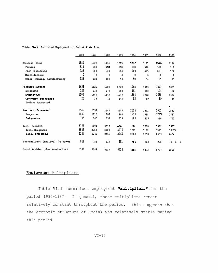
Table VI.3: Estimated Employment in Kodiak St@ Area

Resident BasicFishingFish ProcessingMiscellaneousOther (mining, manufacturing)

Resident SupportExogenousEndogenousGovermtent sponsoredEnclave Sponsored

Resident GoverrmnentExogenousEndogenous

Total ResidentTotal ExogenousTotal Endogenous

Non-Resident (Enclave) En@oyn)ent

Total Residant plus Non-Resident

1980 1981 1982 1983 1984 1985 1986 1987

1580518726

0336

1653124

150525

25451840705

577835432234

818

6596

1310518669

0123

1626130

146333

25581812746

549432522242

755

6249

1174518548

0108

1898179

164772

25441807737

561631602456

619

6235

1215518604

093

2243253

1847143

25871808779

1237518669

050

1968191

169483

25961793803

32762769

681

6726

32212580

754

6555

1195518623

054

1963182

171269

26121795817

577031722598

703

6473

1346518803

025

1873174

163069

26531793860

587233132559

905

6777

1274518721

035

1883162

167249

0

25301787743

56873223 .2464

8 1 3

6500

EmDlovment Multipliers

Table VI.4 summarizes employment ~Fmultiplierst’ for the

period 1980-1987. In general, these multipliers remain

relatively constant throughout the period. This suggests that

the economic structure of Kodiak was relatively stable during

this period.

VI-15

Table VI.4: Smnary of Employment Multipl i era, Kodiak Study Area, 1980-1987’

1980 1981 1982 1983 1984 1985 1986 1987

Endogenoua Employment Hultipl i era[EMEDREEX/EMREEXl 0.41 0.44 0.51 0.55 0.51 0.53 0.48 0.51

Locai Goverment En@oyn’ientMutt ipl iar [EMLGLR/EMEXTOl 0.06 0.06 0.06 0.04 0.07 0.07 0.07 0.06

Stata Govarment En@oymentMultiplier [EMSG/EMEXTO] 0.05 0.06 0.07 0.07 0,07 0.07 0.06 0.06

Stata-Supported ConstructionMultiplier [EMCOSS/EMEXT03 0.0! O.O1 0.02 0.04 0602 0.02 0.02 0.01

State-Supported LocalGovernment Employment Multiplier[EMLGSS/EMEXTOl 0.06 0.06 0.06 0.06 0.07 0.07 0.07 0.06

Po?malation Assunmtiions

Table VI.5 summarizes available population data for the period

1980-1987, as well as our population assumptions for this period. As

discussed previously under Study Area, we have attempted to study the

area around Kodiak connected by roads. For estimating population, we

used the Kodiak Island Borough population as a base then, based on

historical relationships, we adjusted it downward by 10 percent to

compensate for residents of the borough who live outside the study

area. Our 1980 assumption for total population was based on the 1980

census. Our assumptions for 1981-1987 are based on the Alaska

VX-16

Department of Labor’s population estimates.

Our age distribution assumptions are based on the 1980 census.

We assume that this age distribution remains constant throughout the

projection period.

The ratio of assumed resident population to assumed resident

exogenous employment increased from 2.29 in 1980 to 3.21 in 1987.

The fact that this ratio increased gradually suggests additionalo

endogenous employment

better data we assume

at the 1987 level.

and/or higher unemployment. In the absence of

that in the future this ratio remains constant

VI-17

Table VI.5: Population Data for Kodiak Study Area, 1980-1987

1980 1981 1982 1983 1984 1985 1986 1987

Por)ulation Data

1980 census

by age group0-45-1920-64&+

City of KodiakKodiak Island BoroughKodiak Study Area (estimated)

.

Permanent Fund DividendDistributions

Kodiak Island BoroughRoad-connested Area (est’cl.)

Powlation ASSUIU t i onaResident Population: TotalAge Distribution (percant)

Pre-SchooL (O-4)School-age (5-19)Adult (20-64)Senior (65+)

Resident Exogenous EmploymentRatio of Resident Population toRasident Exogenous En@oyment

2716

2656611740

50

4756 4678 5873 5964 6069 6173 6279 63869939 10289 12575 12611 12850 12952 13561 136588945 9260 11318 11350 11565 11657 12205 12292

9656 9205 9132 9~58420 8026 7963 8489

8127 8505 9629 9602 9730 9859 10170 10331

0.100.250.630.03

3543 3252 3160 3276 3221 3172 3313 3223

2.29 2.62 3.05 2.93 3.02 3.11 3.07 3.21

V I - 1 8

Base Case Projections

Figure VI.2 and Table VI.6 summarize our base case projections

,for Kodiak. Total population rises gradually over the projection

period. This is due primarily to increasing tourism.

VI-19

.

Figure VI-2: Kodiak Base Case Projections

KODI,4KEASE CASE EMPLOYMENT ANCIPCIPUL4TION

13 I

I7b–~-””, J

I./w . , ‘“t”lEm~i-@ - -~.,,~,

6,

5 Resident Employment

4

3-1

q*

L~rnrnx-:z-x-.mx..mx!.1 . . . Enclave Emplo~ent k Papulatian

.% -- .“” :.. .,. :m ..-,. x. .A”:4-

-,- YE4R

VZ-2CI

Table VI.6: Stnrnary of E@oyrnent and Population Projectionsfor Base Case

EMPLOYMENT POPULAT IONTotal,

Enc 1 ave ResidentResident Resident Resident Fish- Encleve Enclave and

YEAR Non-OCS Ocs Total Process. Ocs Total Enclave Resident Enclave Total19801981198219831984198519261987198a1989199019911992199319%19951996199719981999200020012002200320042005200620072008200920102011201220132014201520162017201820192020

577854945616604558015770587256875618556855975593562056235602564651%5561556~5689566856535638566356555654565056505650568356825693570457165728580658185830584258555868

00000000000000000000000000000000000000000

57785494561660455801577058725687561855685597559356205623560256465645561556~5689566856535638566356555654565056505650568356825693570457165728580658185830584258555868

818755619681754703905813812812812812812812812812812812812812812812812812812812812812812812812812812812812812812812812812812

00000000000000000000000000000000000000000

818755619681754703905813812812812812812812812812812812812812812812812812812812812812812812812812812812812812812812812812812

65966249623567266555647367776500644463946423641864466449642864726471644164996515649464796464

64816480ti766476647665096508651965306542655466326644ti56666866816694

81278505962996029no98591017010331102261013310186?01781022810233101961027610273102191032510354103151028910261103071029310291102841028410283103441034110361103821040410426105671058910611106331065710681

818755619681754703905813812812812812812812812812812812812812812812812812812812812812812812812812812812812812812812812812812

894592601131811350115651165712205122921103810945

1099011040110451100811088110851103111136111661112711101110721111911105111031109511096110951115611153llln111941121511238113791140111423114451146911492

VI-21

References

Alaska Department of Commerce and EconomicAn Alaska Communitv Profile, Juneau,

Development, Kodiak:Alaska, 1984.

Alaska Department of Labor, Alaska Population Overview 1985Estimates, April 1987.

Alaska Department of Labor~ Employment Database Files forCordova, Homer, Kenai, Kodiak, Seward, and Yakutat, November1988 (unpublished).

Alaska Department of Labor, Geoura~hical Area ClassificationManual. January 1981.

Alaska Department of Labor, July 1 Population Estimates, NewsRelease, March 1, 1988.

Alaska Department of Revenue, Permanent Fund Dividend RecipientProfiles.

Fried, Neal, “Employment in Alaska’s Seafood Industry,” AlaskaEconomic Trends, Juneau, Alaska: Alaska Department of Labor,July 1987.

Fried, Neal, The Center of Alaskars Bottomfish Grounds: Kodiakand the Aleutian Islands,” Alaska Economic Trends, Juneau,Alaska: Alaska Department of Labor, July 1988.

Keiser, Gretchen, and Pierce, Brad. State of Alaska Budqet, FY 84-FY 87. Alaska State Legislature, House Research AgencyReport 87-C, February 1987.

Knapp, Gunnar; Nebesky, W.; Hull, T.; White, K.; Reeder, B. ; andZimicki, J. Gulf of Alaska Economic and DemoaraDhic SystemsAnalvsis. University of Alaska, Institute of Social andEconomic Research, (Prepared for Minerals and ManagementService, Alaska OCS Office) Social and Economic StudiesProgram, Technical Report Number 98, March 1984.

Livey, Jay, and Keiser, Gretchen. Public School Financinq inAlaska. Alaska State Legislature, House Research AgencyReport 87-A, February 1987.

United States, Department of the Interior. Technical Report Number122: A Descri~tion of the Economic and Social Svstems ofthe Kodiak-Shumaain Reaion. Anchorage: CulturalDynamics Ltd., 1986.

U.S. Census, 1980.

VI-22

CHAPTER VII: DESCRIPTION AND MODEL ASSUMPTIONS: SEWARD

Overv iew

Seward is located at the head of Resurrection Bay. It is

Alaska’s only deep water, ice-free port that has rail, highway,

and air links to the major urban areas and the interior of the

state. Seward is 127 miles south of Anchorage by highway and 35

minutes by air. The Alaska Marine Highway System provides ferry

service to Seward.

Seward, with a population of 2,324 in the city, and an esti-

mated 996 in the outlying area, has a diverse economy for a city

its size. The economy is supported by fish processing, a coal

export facility, and the state’s long-term maximum correctional

center. A wood products plant is to begin production this year.

Ship services and repairs and a vocational training facility are

available in Seward. The University of Alaska’s Institute of

Marine Science and the headquarters for the Kenai Fjords National

Park are also located in Seward.

Government is an important employer, providing over 30

VII-1

percent of

operations

recreation

Total

employment in 1987. This increased significantly with

of the Spring Creek Correctional Facility. Tourism and

are also an important part of the economy.

employment in Seward. increased slightly between 1980

and 1987 with more significant growth in retail trade and

services. State government employment increased substantially

after the Spring Creek Maximum Correctional Facility began

operations.

Maior Data Sources

The primary data source for our analysis of Seward was

Department of Labor data on employment for Seward. In addition we

referred to Citv of Seward Com?uehensive Plan (November 1985) ;

‘fCity of Seward Community Profile” (undated) ; and “Gulf of Alaska

Economic and Demographic Systems Analysis,’t Social and Economic

Studies Program, Technical Report Number 98, March 1984 (subse-

quently referred to as TR 98). We also discussed current develop-

ment projects in Seward with Gary Martin, City of Seward. We have

listed all of the sources used in our analysis at the end of this

chapter.

VII-2

Studv Area

Figure VII.1 shows the area which we are defining as Seward.

Our employment and population assumptions and projections for this

study refer to employment and population within this area. This

area corresponds approximately to the “sub-sub area!’ used by

Department of Labor for employment s t a t i s t i c s .

EmDlovment Assum~tions

Table VII.1 shows Alaska Department of Labor employment data

for Seward for the years 1980-1987. These data formed the primary

basis for the development of our employment assumptions, and are

the basis for all employment data not otherwise cited.

We made additional assumptions to account for industries not

included in the Department of Labor data (e.g. fish harvesting) or

which were fully or partially suppressed (e.g. manufacturing and

wholesale trade) , and to allocate employment within a given

industry between resident and enclave shares, exogenous and

endogenous shares, etc. Our resulting employment assumptions for

the years 1980-1987 are shown in Table VII.2. Below we discuss

these assumptions by industry.

VII-3

. .

Figure VII-1: Seward Study Area, ---------- ,,..7 .- .--.-—--~JlnellM.cO@nlk.l -.,. +.J__.., o; ,$

=?.K+i-wii%’.: ,,,,.}4(1

. .

*--- .

Table VII.1: Smmsry of Department of Labor En@oymant Data for Seward

Cate90rv Code 1980 1981 1982 1983 1984 1985 1986 1987

MiningConstruct ionManufacturingTrans., Ccmm, UtilitiesIJholesaie TradeRetail TradeFin., Ins., & Rest EstateServicesForestry, Ag., FisheriesFederal GovernmentState GovernmentLoca 1 GovernmentTOTAL

1 * * ●

2 32 * 193 * * ●

4 45 48 735 * * *6 137 126 1427 17 20 208 167 169 1989 * * ●

10 34 31 3311 194 203 22212 109 112 121

1205 1107 1176

*

43●

39*

13419

195*

35216134

1072

* o 0 062 32 73 101* * * *

96 138 98 60* * 42 46

137 146 160 ●

22 23 22 21201 236 218 *

* * * *42 36 37 37

229 241 221 208141 154 169 175

1171 1229 1218 1234

* Data suppressed.

VII-5

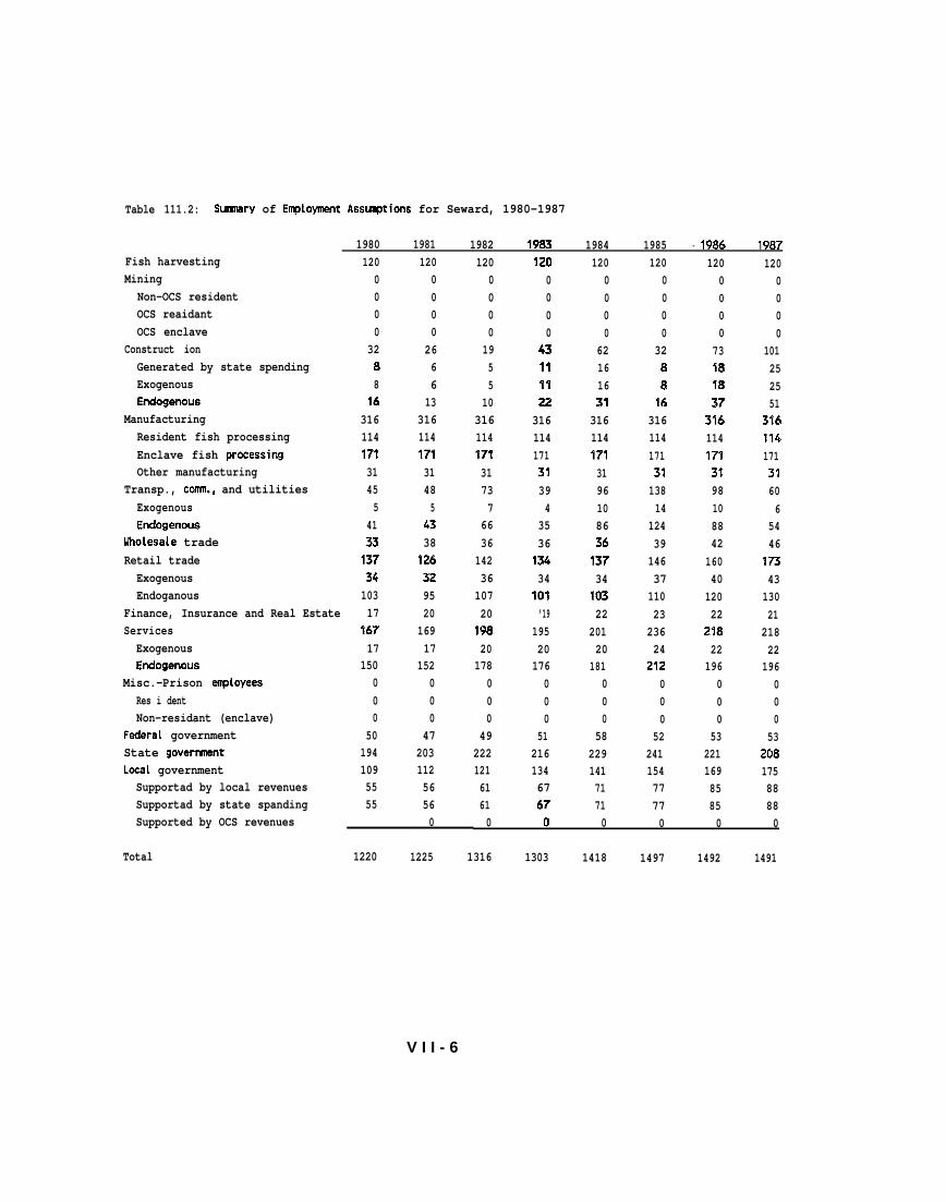
Table 111.2: Smmary of En@oymant Assmpticm for Seward, 1980-1987

1980 1981 1982 1983 1984 1985 -1986 1987Fish harvestingMining

Non-OCS residentOCS reaidantOCS enclave

Construct ionGenerated by state spendingExogenousEndoganous

ManufacturingResident fish processingEnclave fish proceaaingOther manufacturing

Transp., ccmn., and utilitiesExogenousEndogenous

Uholesale tradeRetail trade

ExogenousEndoganous

Finance, Insurance and Real EstateServices

ExogenousEndogenoua

Misc.-Prison an@oyeesRes i dentNon-residant (enclave)

Fadaral governmentState goverrmnantLocaL governmentSupportad by local revenuesSupportad by state spandingSupported by OCS revenues

1200000

328816

31611417131455

41331373410317

16717

150000

501941095555

1200000

266613

31611417!31485

4338126329520

16917

152000

4720311256560

1200000

1955

1031611417131737

6636

142361072019820

178000

492221216161

1200000

431$1122

31611417131394

353673434

101’19

19520176

000

512161346767

1200000

62161631

31611417131961086361373410322

20120

181000

582291417171

1200000

328816

3161141713713814

124391463711023

23624

212000

522411547777

1200000

731$1837

3161141773198108842

16040

12022

2?822

196000

532211698585

1200000

101252551

31611417137606

5446

1734313021

21822

196000

532C181758888

0 0 0 0 0 0

Total 1220 1225 1316 1303 1418 1497 1492 1491

V I I - 6

Fish Harvesting

Seward is a center of fishing and fish processing for Prince

William Sound and the Gulf of Alaska. Seward residents held 362

fish permits according to Seward’s ‘lOn the Movet~ brochure.

Alaska Department of Labor data was suppressed for “forestry,

agriculture, and fisheries.” In 1980, resident fish harvesting

employment (FTE) was 120 (TR 98). Although this may understate

full-time fish harvesting employment in more recent years, we have

assumed this figure for the period 1980-1987. We have also

assumed that fish harvesting employment will remain constant at

this level for the period 1988-2020.

Mininq

Non-OCS Resident. Mining employment data was suppressed for

1980 through 1984. In 1985-1987 mining employment was shown at

zero (Table VII.1). Thus, we have assumed that non-OCS mining

employment was zero for the entire period 1980 through 1987 and

will remain at zero.

OCS Mining. We have assumed zero OCS mining employment in

VII-7

the Kenai Market Area during the period 1980-1987. Similarly, our

“base case” model assumptions assume zero OCS mining employment

during the period 1988-2020.

Construction

Construction projects during the

Spring Creek Correctional Facility, a

fish processing plant and ship repair

completion is the Chugach Development

19808s have

coal export

facilities.

included the

facility,

Nearing

Corporation’s $12 million

wood products saw mill and scheduled to begin construction

during 1988-1989 are a new fish processing plant and a ship

repair facility.

Construction employment increased from 32 in 1980 to 101 in

1987 (Table VII.1). We assumed that 25 percent of construction

employment during the period 1980-1987 was supported by state

government capital spending, 25 percent was exogenous, and 50

percent was endogenous, based on our best judgment in the absence

of any data.

We assumed exogenous employment of 25 during the period 1988-

2020, based on on our best judgment in the absence of any data.

VII-8

Manufacturing

Fish Processing Employment. Fish processing is the primary

type of manufacturing in Seward. Department of Labor manufac-

turing employment data were suppressed for 1980 through 1987

(Table VII.1). TR 98 showed resident fish processing employment

(FTE) in 1980 of 114. Assuming that the resident share for fish

“processing employment is .4, then non-resident fish processing

employment is estimated at 171 (Table VII.1).

We assumed that fish processing employment will increase by

90 to 375 during 1990-2020 due to operation of a new fish

processing plant.

Wood Products. We assume that the new Chugach Forest

Products, Inc. sawmill, which is scheduled for completion in July

1989, will create additional manufacturing employment of 50

according to testimony by Paul Tweeten, Timber Division Manger,

Chugach Forest Products at the House Resources Committee hearing

(Wasilla March 11, 1989). We assume that wood products employment

will remain at 50 for 1989-2020.

VII-9

Transportation, Communications, and Utilities

Average annual employment in transportation, communications

and utilities ranged from 45 in 1980 to 138 in 1985~ and then

declined to 60 in 1987 (Table VII.1). We assumed that 10 percent

of employment in this industry was exogenous and 90 percent was

endogenous. We assumed that exogenous transportation, communica-

tions and utilities employment will grow at 5 percent per year

after 1987, based on the assumption that economic activity related

to tourism and sports fishing in the Seward area will continue to

expand.

Wholesale Trade

Wholesa le

(Table VII.1).

of total trade

1980-1985 based

wholesale trade

Retail Trade

trade employment was 42 in 1986 and 46 in 1987

In 1986, wholesale trade comprised 20.79 percent

. We estimated wholesale trade for the period

on this relationship. We assumed that all

employment was endogenous.

Retail trade average annual employment ranged from 137 in

1980 to 160 in 1986 (Table VII.1). The 1987 retail trade figure

VII-10

was suppressed and, since wholesale trade was shown for 1987,

retail trade was estimated based on the relationship discussed in

the preceding section “wholesale trade.!c We assumed that 25

percent of retail trade employment was exogenous and 75 percent

was endogenous. We assumed that exogenous retail trade employment

will grow at a rate of 5 percent per year after 1987.

Finance, Insurance, and Real Estate

Average annual employment in ‘tF.I.R.E.” increased from 17

employees in 1980 to 23 in 1985 then decreased to 21 in 1987

(Table VII.1). We assumed that all employment in these industries

was endogenous.

Services

Annual average employment in services increased from 167 in

1980 to 236 in 1985 then declined to 218 in 1986 (Table VII.1).

Since services employment for 1987 was suppressed, we assumed it

to be the average of employment in 1984-1986, a value of 218. We

assumed that 10 percent of employment in this industry was exoge-

nous and 90 percent was endogenous. For the IIbase casell scenario,

we assumed exogenous employment in services will grow at a rate of

5 percent per year during 1988-2020.

VII-11

Federal Government

Civilian federal government employment in Seward increased

from 34 in 1980 to 42 in 1984 then decreased to 37 in 1986 and

1987 (Table VII.1). The U.S. Coast Guard stations 16 personnel on

a 110 foot vessel in Seward. Seward has been vying ho become a

U.S. Navy home port. However, since it.

Navy and the State of Alaska are unable

who will finance the project, we assume

home port project in Seward. We assume

appears that the U.S.

to reach an agreement on

that there will not be a

federal government employ-

ment is exogenous and thus project it at the 1987 level for 1988-

2020.

State Government

State employment increased from 109 in 1980 to 175 in 1987

(Table VII.1), State employment is assumed to be totally

endogenous with the exception of the Spring Creek Correctional

Facility. We assume that employees at this maximum security

prison are exogenous. Thus , in the model, Spring Creek employment

is shown separately.

Operation of the Spring Creek

VII-12

Correctional Facility began in

1988 with a work force of 200. According to the City of Seward,

many of these employees transferred to the Spring Creek facility

from other parts of the state. It is our understanding that many

of these employees commute during their off-time to residences

elsewhere. We assume that these employees and their families are

trying to sell their homes in order to relocate permanently to

Seward but that this “adjustment” period may be prolonged because

of the poor housing market in the state. Therefore, for 1988-1990

we showed a decreasing proportion of Spring Creek employees as

non-resident employees. We assume that these non-residents are,

for example, sharing apartments with other employees in similar

situations and maintaining households and families elsewhere in

the state. We assume that after 1990 all the Spring Creek

employees will be permanent residents of Seward. We also assume

that employment at this facility will remain stable at 200 during

1988-2020.

Local Government

Local government employment increased from 109 employees in

1980 to 175 employees in 1987 (Table VII.1). Local government

employment includes components “supported by state spending” and

Ilsupported by local revenues” which we assume to be endogenous.

It also includes “local government supported by OCS revenues.”

VII-13

Table VII.3: Estimated EnqJloymant in Seward

Resident BasicFishingFish ProcessingMisc. and PrisonOther (mining, manufacturing)

Resident SupportExogenousEndogenousGovernment SponsoradEnclave Sponsored

Resident Government*ExogenousEndogenous

Total ResidentTotaL ExogenousTotal Endogenous

Non-Resident (EncLave) Enqdoymant

TotaL Resident plus Non-Resident

*

1980 1981 1982 1983 1984 1985 1986 1987

2651201 ?4

o31

43763

3608

35350

303

1049378671

171

1220

265120114

031

42760

3616

36247

315

1054372682

171

1225

265120114

031

48867

4165

39249

343

114538176

171

1316

2651201140

31

46668

38811

40151

350

1132384748

171

1303

265120114

031

55479

45916

42858

370

1247402845

171

1418

265120114

031

61482

5244

44752

395

1326399927

171

1497

265120114

031

61390

50518

44353

390

1321408913

171

1492

Ooes not include employment at the prison, which is included under Resident Basic.

This category is exogenous and we assume for the base case

scenario that it is zero for 1988-2020.

Em~lovment Multi~liers

265120114

031

61996

49725

43653

383

1320414906

171

1491

Table VII.4 summarizes employment ltmultipliersl! for the period

VII-14

1980-1987. In general, these multipliers fluctuate substantially.

This suggests that either the economic structure of Seward was

fluctuating substantially during this period, or (more likely) our

employment assumptions are unreasonable for some years. However,

our assumptions nevertheless remain our best estimates given the

limited available employment data.

Table VI I.4: Smmsry of Employment Multipliers, Sewerd, 1980-1987

1980 1981 1982 1983 1984 1985 1986 1987

Erogenous Employment Multi pliers[EMEDREEX/EMREEXl

Local Government EmploymentMultiplier [EMLGLR/EMEXTOl

State Goverrunant E@oyrnentMulti plier [EMSG/EMEXTOl

State-Supported ConstructionMultiplier [EMCOSS/EMEXTOl

State-Supported LocalGoverment Employment Multiplier[EHL=WENEXTO1

0.93 0.95 1.07 0.99 1.12 1.29 1.22 1.18

0.10 0.10 0.11 0.12 0.12 O.lA 0.15 0.15

0.35 0.37 0.40 0.39 0.40 0.42 0.38 0.36

0.06 0.05 0.03 0.08 0.11 0.06 0.13 0.17

0.10 0.10 0.11 0.12 0.12 0.14 0.15 0.15

Population Assum~tions

Table VII.5 summarizes available population data for Seward for

the period 1980-1987, as well as our population assumptions for this

period. Our 1980 assumption for total population was based on the

VII-15

1980 census. Our assumptions for 1981-1983 are based on Department

of Labor, Alaska Population Overview publications. For 1984-1987 we

used population numbers from the City of Seward.

Our age distribution assumptions are based on the 1980 census.

We assume that this age distribution remains constant throughout the

projection period.

The ratio of assumed resident population to assumed resident

exogenous employment increased from 6.80 in 1980 to 7.60 in 1987.

The fact that this ratio was relatively constant suggests that our

assumption is a reasonable one that this ratio remains constant for

future years at the 1987 level.

V I I - 1 6

Table VI I.5: Population Data for Seward, 1980-1987

1980 1981 I 982 1983 1984 1985 1986 1987

Population Data

1980 census 1843

by age groupo-4 1285-1920-6465+ 144

Alaska Population OverviewSeward, city 1843 1943 1839 1925

City of SewardSeward, city 2072 2175 2223 2324Populated area outside city (est’s) 900 900 900 900 900 935 953 996

Total Seward area population

Permanent Fund DividendDistributions

AdultChildren

School Enro(iment

Population AsstqtionsResident Po~lation: TotalAge Distritmion (PWCeflt)

Pre-School (O-4)School-age (5-19)Adult (20-64)Senior (65+)

Resident Exogenous EmploymentRatio of Resident Population toResident Exogenous En@oyrnent

2743 2843 2739 2825 2972 3110 3176 3320

2877 2i32 2823 30812156 2057 2089 2276721 675 734 805

472 453 511 561 586 585

2572 2672 2568 2654 2801 2937 3005 3149

0.070.210.640.08

378 372 38T 384 402 399 408 414

6.80 7.19 6.73 6.92 6.96 7.36 7.37 7.60

VII-17

Base Case Projections

Figure VII.2 and Table VII.6 summarize our base case projections

for Seward. Total population rises gradually over the projection

period. This is due primarily to increasing tourism and assumed

expansion of the industrial base.

VII-18

. .

.3

7

6

5

4

~

2

1

Figure VII-2: Seward Base Case Projections

~ EIJ/:&R ~

EWE CASE EMPLCIYMENT AND POPULATION

..4I xsdcmt Employment

ave Employment & Populatmn

o1980 1985 1990 1995 2000 2005 2010 2015 2020

YEAR

VII-19

Table VI 1.6: Sunnary of En@oymant and Population Projections for Base Case

EMPLOYMENT POPULATIONTotal,

Enc 1 ave ResidentResident Resident Resident Fish- Enclave Enclave snd

YEAR Uon-OCS Ocs Total Process. Ocs Total Enclave Resident Enclave Tota 1198019811982198319841985198619871988198919901“9911992199319941995199619971998199920002001200220032004200520062007

200920102011201220132014201520162017201820192020

104910541145113212471326132113201792186320082123216221782172223122452231230623402337234123452392

2427244524702494255825842625266927142761281128622916297230313092

00000000000000000000000000000000000000000

10491054114511321247132613211320179218632008212321622178217222312245223123062340233723412345239224062427244524702494255825842625266927142761281128622916297230313092

171171171171171171171171225225225225225225225225225225225225225225225225225225225225225225225225225225225225225225225225225

00000000000000000000000000000000000000000

171171171171171171171171375325275225225225225225225225225225225225225225225225225225225225225225225225225225225225225225225

122012251316130314181497149214912167218822832348238724032397245624702456253125652562256625702617263126522670269527192783280928502894293929&$303630873141319732563317

25722672256826542801293730053149430044704819509551895228521453535387535455355616560956195627574257735824586959285986614062016301

65146627674668696998713372747422

171171171171171171171171375325275225225225225225225225225225225225225225225225225225225225225225225225225225225225225225225

274328432~928252972310831763320480351155414564057345773575958985932589960806161615461646172628763186369641464736531668567466846695070597172729174147543767878197967

VII-20

References

Alaska Department of Labor, Alaska Po?mlation Overview 1985Estimates, April 1987.

Alaska Department of Labor, Employment Database Files forCordova, Homer, Kenai, Kodiak, Seward, and Yakutat, November1988 (unpublished).

Alaska Department of Labor, Geoaranhical Area ClassificationManual. January 1982.

Alaska Department of Labor, July 1 Population Estimates, NewsRelease, March 1, 1988.

Alaska Department of Revenue, Permanent Fund Dividend ReciDientProfiles, 1982-1985.

Alaska Transportation Consultants, Inc.; CCC Architects andPlanners; Kevin Waring Associates. Seward Aimort Land Useand Development Plan, Final Re~ort. Prepared for the City ofSeward. December 1985.

CCC Architects Alaska, Kevin Waring Associates, and AlaskaTransportation Consultants, Citv of Seward ComprehensivePlan, Adopted by the Kenai Peninsula Borough, November 5,1985.

Chemical Bank, Information Memorandum. Seward Marine IndustrialCenter, March 6, 1985.

Kenai Peninsula Borough, Situation and Prospects, 1985, 1986, May1987, August 1988.

Keiser, Gretchen, and Pierce, Brad. State of Alaska Bud~et. FY 84-FY 87. Alaska State Legislature, House Research AgencyReport 87-C, February 1987.

Martin, Gary. City of Seward. Telephone Interview. October 28,1988.

Merritt, R. D., “Public-Data File 86-95, The Seward Coal Terminal1985,” Alaska Division of Mining and Geological andGeophysical Surveys, December 1986.

National Park Service, Anchorage, Alaska, Draft EnvironmentalImnact Statement for the Wilderness Recommendation, KenaiFiords National Park, Alaska, 1988.

Seward, Alaska, Detailed Proiect Re~ort and Final EIS for ProposedSmall Boat Harbor Navigational Im?novements, Amendix B.

VII-21

Economics, April 1982.

Seward, City of, “On the Move... A Community Profile,” (Undated).

U.S. Census, 1980.

,:,

VII-22

. .

CHAPTER VIII. DESCRIPTION AND MODEL ASSUMPTIONS: YAKUTAT

Overview

Yakutat is a fairly self-contained community without close

economic relationships with other communities, the nearest of

which is Cordova (225 miles northwest) . There are daily air

connections between Anchorage (380 air miles) and Juneau (225 air

miles) . Yakutat Bay opens to the unprotected waters of the Gulf

of Alaska, making regular access to Yakutat possible only by

ocean-going vessels. The Alaska Marine Highway System does not

serve Yakutat.

Commercial fishing and seafood processing dominate the

economy. In addition there is a small amount of logging. One of

the principal reasons that Yakutat was originally established as a

town was fishing. A cannery was constructed which drew workers

the site. Fishing is a way of life in Yakutat; a ‘Traditional

occupation acknowledged by the community” (OEDP Update, 1988) .

Government is the second most important sector in the

economy, providing stable year-round employment. The community

to

is

encouraging tourist and recreation oriented businesses, particu-

VIII-1

larly emphasizing the world-class sport fishing offered in the

Situk River. According to the OEDP Update (1987):

“A 1987 study prepared for the Alaska Division of Sport

Fisheries estimates 6,581 sport fishing trips were made in

1986 in the Yakutat area, with a total of 11,020 days

fished. ..” (ibid., p. 19)

Total employment in Yakutat increased slightly between 1980

and 1987.

Mafior Data Sources

The primary data source for our analysis of Yakutat was

Department of Labor data on employment for Yakutat. In addition

we refer to the Overall Economic Development Proaram, 1988 Update,

the Yakutat Comprehensive Plan (November 1983); the Yakutat

Airnort Master Plan Renort (December 1987); and lrGulf of Alaska

Economic and Demographic Systems Analysis,it Social and Economic

Studies Program, Technical Report Number 98, March 1984 (subse-

quently referred to as TR 98). We spoke with Carla Moore, a

Planner with the City, who was very helpful in providing

information.

VIII-2

We have listed all of the sources used in our analysis at the

end of this chapter.

Studv Area

Figure VIII.2 shows the area which we are defining as

‘aYakutat .“ Our employment and population assumptions and

projections for this study refer to employment and population

within this area. This includes the City of Yakutat and the

surrounding road connected area and approximately corresponds to

the sub-sub area used by Department of Labor for employment

statistics.

EmDl ovment Assumptions

Table VIII.1 shows Alaska Department of Labor employment data

for Yakutat for the years 1980-1987. These data formed the

primary basis for the development of our employment assumptions,

and are the basis for all employment data not otherwise cited.

We made additional assumptions to account for industries not

included in the Department of Labor data (e.g. fish harvesting) or

which were fully or partially suppressed (e.g. manufacturing and

wholesale trade) , and to allocate employment within a given

VIII-3

Figure VIII-1: Yakutat Study Area

.

. .

Source: ~. S. Buesuot~he Cenms

A. Skagway - Yakutat - Angoon Census Area

,. . .. ..

Adaated from AEIDC AK Regionai Pro filee

B. (Xty of Yakutat

Note: The study area for our descriptions and pro j ections is the areaconnected by road to the community of Yakutat. Most people live withinfive miles of the community.

industry between resident and enclave shares, exogenous and

endogenous shares, etc. Our resulting employment assumptions for

the years 1980-1987 are shown in Table VIII.2. Below we discuss

these assumptions by industry.

Table VII I. 1: Winery of Department of Labor En@oyment Data for Yakutat

Categow Code 1980 1981 1982 1983 1984 1985 7986 1987

Mining 1Construction 2Manufacturing 3Trans., Comn., Utilities 4Wholesa Le Trade 5Retail Trade 6Fin., Ins., & Real Estate 7Services 8Forestry, Ag., Fisheries 9Federa 1 Government 10State Goverrmnent 11Loca 1 Goverrmnent 12TOTAL

o 0 0 0 0 0 0 0* * ● * * * ● ** * 55 57 54 * * *13 13 13 21 29 29 27 17* * * * * * * o

28 24 22 25 26 25 34 34* 13 15 15 13 10 12 ** * * 20 19 20 27 250 0 0 0 ● * * *

19 19 18 18 16 16 16 180 0 0 0 0 0 0. 0

48 51 53 53 55 59 59 58164 216 209 215 221 200 222 174

* Data Suppressed.

VIII-5

Table VI II.2: Sunmsry of Employment Assumptions for Yakutat, 1980-1987

1980 1981 1982 1983 1984 1985 1986 1987Fish harvestingMining

Non-OCS residentOCS res i dentOCS enclave

Construct ionGenerated by state spendingExogenousEndogenous

Manufacture ingResident fish processingEnclave fish processingOther manufacturing

T ransp., coinnunications, utilitiesExogenousEndogenous

Uhotesaie tradeRetail trade

ExogenousEndoganous

Finance, insurance and Reai EstateServicesExogenousEndogenous

Misc. ‘LoggingRes. LoggingEnclave Logging

FedersL governmentState goverrnientLocal government

Supported by local revenuesSupported by state spendingSupgmrted by OCS revenues

Total

380000211!

415

315

131

121

283

2513121

11391029196

4824240

3800003112

5514410

131

121

242

2213141

13391029196

5126260

3800003112

S!i14410

131

121

222

2015171

16391029186

5327270

3800003112

57’14430

211

201

2532315201

1939102918115327270

3800003112

5414410

291

281

263

2313191

1839102916115528280

3800002111

5013380

291

281

253

231020f

1939102916115930300

3800003112

5614420

271

262

343

3112’271

2639102916115930300

3800002111

4411330

171

160

343

3112251

243910291811582929J

260 2?6 280 301 304 300 324 298

VIII-6

Fish Harvesting

According to Yakutat’s OEDP U~date (1988):

ltIn 1987 Commercial Fisheries Entry Commission issued 118

commercial setnet permits, 58 hand troll permits and five

power troll permits to people who show Yakutat as their place

of residence. Based upon this number of issued permits, and

local knowledge of crewmember participation, it is estimated

that over 150 residents of Yakutat fish commercially.”

“Sitka Sound Seafoods, based in Sitka, AK, has leased both

processing sites from the City. A well known operation, they

have drawn a larger number of fishing boats to Yakutat. Thus

far into the 1988 season they have maintained a crew of 50-70

depending on volumes of product going through the plant.’t

!!Rainier Seafoods,a Seattle based company, has leased from

Yak-Tat Kwaan the site previously used as an oil-service

base. ..”

The Alaska Department of Labor showed the ‘~forestry,

agriculture, and fisheries” category with zero employment in 1980

VIII-7

through 1983 (Table VIII.1). This category should include fish

harvesting employment. The 1980 census counted 16 employed

persons claiming forestry, fishing, or farming as an occupation TR

98). Xn TR 98, it is speculated that . . . Isa significant portion Of

Yakutat’s resident, licensed fishermen could have been omitted

from the [1980] census tabulations because they were not actually

working in the designated time period of the survey...’~ and an

FTE figure of 38 is used. The Yakutat OEDP Update (1988, p. 17)

estimates that over 150 residents” fish commercially but seasonal-

ly . Coughenower (Commercial Fishina Industrv Studv , Homer,

Alaska) states that one seasonal fish harvesting job (in Homer)

averages 2.4 months in duration. If this relationship is also

applicable to Yakutat, then full-time equivalent fish harvesting

employment would actually be 30. In the absence of any other

data, we have assumed 38 FTE fish harvesting employees for the

period 1980-1987. We have also assumed that fish harvesting

employment will remain constant at this level for the period 1988-

2020.

Mininq

Non-OCS Resident. Little if any mining or mineral

development is currently occurring in the Yakutat area. The

Alaska Department of Labor omits mining; thus we assume that

VIII-8

mining employment is zero (Table VIII.1). Development of offshore

gold dredging has been discussed within the community although we

do not know of any actual plans to begin production.

We

through

assume that non-OCS mining employment was zero from 1980

1987 and that it will remain at zero during the period

1988-2020.

OCS Mininq. We have assumed zero OCS mining employment in

Yakutat during the period 1980-1987. Similarly, our “base case”

model assumptions assume zero OCS mining employment during the

period 1988-2020.

Construction

The Alaska Department of Labor figures were suppressed

(Table VIII.1). In 1987, construction employment in the Skagway-

Yakutat-Angoon Census Area was 1.2 percent of total employment.

We assumed that this relationship was also valid for the Yakutat

sub-sub area and estimated construction employment of between two

and three for the years 1980-1987 (Table VIII.2).

We assumed that 25 percent of construction employment during

VIII-9

the period 1980-1987 was supported by state government capital

spending, 25 percent was exogenous, and 50 percent was endogenous,

based on our best judgment in the absence of any data.

We assumed exogenous employment of 3 during the period 1988-

2020, based on on our best judgment in the absence of any data.

Manufacturing

Fish Processing Emnlovment. Manufacturing in Yakutat is

primarily fish processing. Sitka Sound Seafoods leased two

processing sites from the city, During the 1988 season there was

a crew of 50-70. Raihier Seafoods (Seattle) leased, a plant site

and will apparently be processing seafood this year (Yakutat OEDP

Update, 1988, p. 18).

Department of Labor showed employment levels only for

1982-1984--55 employees in 1982, 57 in 1983, and 54 in 1984

Table VIII.1). Manufacturing employment was between 24 and 26

percent of the total Department of Labor employment figure. In

comparison, in 1980, 33 residents and

employed in fish processing on an FTE

IIotherlt manufacturing (TR 98) . There

one non-resident were

basis; there were 5 FTE’s in

is no manufacturing other

than fish processing in Yakutat. Thus we show arotherll

VIII-10

manufacturing as zero in 1981 through 1987 (Table VIII.2) .

One seafood processor in Yakutat had 20 percent of total

hours worked by residents and 80 percent by non residents during

June through September 1988. The resident share was about 38

percent during

resident share

resident share

April and May 1988. In comparison, in 1980 the

was assumed to be .8 (TR 98), We assume that the

of fish processing employment at .25 during the

period 1980-1987. Resident fish processing employment is thus

shown at 11 and non-resident fish processing employment at 33 in

1987 (Table VIII.2).

We assumed that both resident and non-resident fish

processing employment will remain constant at the

during the period 1988-2020.

Trans~ortation, Communications, and Utilities

Employment in transportation, communications

increased from 13 in 1980 to 29 in 1984 and 1985,

17 in 1987 (Table VIII.1).

employment in this industry

endogenous. We assumed that

1987 levels

and utilities

then declined

We assumed that 5 percent of

was exogenous and 95 percent was

exogenous

cations and utilities employment will

VIII-11

transportation, communi-

grow at 3 percent per year

to

after 1987, based on an assumption that economic activity related

to tourism will continue to expand.

Wholesale Trade

wholesale trade figures were suppressed by the Department

of Labor (Table ‘VIII.1). However, in 1980 wholesale trade was

5 percent of total trade. Thus, to estimate wholesale trade

during 1980-1987, we assumed that wholesale trade remained

constant at 5 percent of total trade. Since retail trade

figures were available, wholesale trade

based on these relationships wholesale

1980-1985 and 2 in 1986 (Table VI~I.2)e

employment was estimated

trade is shown at 1 in

In 1987 Department of

Labor showed no wholesale trade employment in Yakutat (Table

VIII’.1) . We assumed that all wholesale trade employment was

endogenous.

Retail Trade

Retail trade average annual employment shown by Department of

Labor decreased from 28 in 1980 to 22 in 1982, then increased to

26 in 1984 and 34 in 1986 and 1987 (Table VIII.1). We assumed

that 10 percent of retail trade employment was exogenous and 90

percent was endogenous. We assumed that exogenous retail trade

VIII-12

employment will grow at a rate of 3 percent per year after 1987.

Finance, Insurance, and Real Estate

Average annual employment in finance, insurance and real

estate ranged between 10 and 15 during 1981 through

were suppressed for 1980 and 1987. We assumed that

employment in 1980 was the same as in 1981 and that

1986. Data

11 FIRE II

employment in

1987 was the average of employment during the preceding three

years (1984-1986) (Table VIII.2). We assumed that all employment

in these industries was endogenous.

Services

Annual average employment in senices ranged between 20 and

27 between 1983 and 1987. Twelve employees were assumed for 1980

(TR 98) (Table VIII.2). Figures were then interpolated for 1981

and 1982. We assumed that 5 percent of employment in this indus-

try was exogenous and 95 percent was endogenous. We assumed that

exogenous services employment will grow at a rate of 3 percent per

year after 1987.

VIII-13

Since 1980 the local timber industry has been a relatively

stable sector of the economy. Timber is harvested primarily

from land owned by Yak-Tat Kwaan, the local native village

corporation. “Kwaan . . . sold the majority of its timber

stumpage rights to Silver Bay Logging which operates the

sorting yard, and sells round logs to buyers. A saw mill was

built by Kwaan in 1983, but other than test runs, it. has never

operated nor is it expected to operate in the future (OEDP

Update, 1988, p. 16).1? According to the OEDP Update, approxi-

mately 50 loggers are employed in Yakutat, of which only 10-15

are local residents. Timber harvesting on Yak-Tat Kwaan lands

is only expected to last for two to three more years. The city

and the U.S. Forest Service are grappling with the trade-offs

between continued timber harvest on federal land with related

economic benefits and protection of fish habitat and promotion

of tourism. The city council has requested that there be no

logging west of the Dangerous River on the Yakutat Forelands.

Logging is also included in the ‘tforestry, agriculture,

and fisheries” category for the Department of Labor’s purposes

in enumerating employment. Yakutat has had a relatively stable

timber industry since 1980 and it is expected to continue for

V I I I - 1 4

the next

loggers,

two to three years--we assume through 1990. There are 50

only 10 to 15 of whom are local residents. In addition,

65 longshoremen work approximately 35 days per year loading

vessels with timber. We estimate that the longshoremen are

equivalent to 9 full-time jobs and that the logging operations

provide 30 full-time-equivalent jobs but the resident share is

only .2-.3. For 1980 through 1987 we assume 10 resident

logging/loading jobs (FTE) and 29 non-resident (enclave) jobs. We

assume that these figures will remain the same for 1988 through

1990 at which time logging employment will be zero. This could,

however, change if logging begins on U.S. Forest Service lands.

Federal Government

Federal government employment in Yakutat between 1980 and

1987 decreased from 19 in 1980 to 16 in 1984-1986. In 1987

federal employment was 18 (Table VIII.1). Federal agencies

located in Yakutat are the U.S. Forest Service, National Park

Service, Federal Aviation Administration,

assume that federal employment is totally

at the 1987 level for 1988-2020.

and the Post Office. We

exogenous and project it

VIII-15

State Government

According to the Department of Labor, there is no state

government employment in Yakutat (Table VIII.1). However, because

the Department of Labor reports employment by census division,

there can be state employment in Yakutat but it ends up in a

different sub-sub area (Airport Plan Phase 1]. In 1980, there

were 6 FTE state employees in Yakutat (TR 98) and a 1983 telephone

survey of Yakutat employers showed 10 state employees. ALaska

Department of Fish and Game and the Department of Transportation/-

Public Facilities both have offices in Yakutat. Thus? we assume

that state employment was 6 during 1980-1982 and 11 for the period

1983-1987.

Local Government

Department of Labor average annual employment data show 48

local government employees for Yakutat in 1980. This increases to

59 in 1985 and 1986 and 58 employees in 1987 (Table VIII.1).

Local government employment includes components ‘supported by

state spending” and “supported by local revenues” which we assume

to be endogenous. It also includes “local government supported by

OCS revenues.” This category is exogenous and we assume that it

is zero for 1988-2020.

VIII-16

Table VIII.3: Estimated Employment in Yakutat

Resident BasicFishingFish ProcessingL099i ngOther (mining, manufacturing)

Residant SupportExogenousEmlogenousGoverrmant Sponsor4Enclave Sponsored

Resident GovernmentExogenousEndogenous

Total ResidentTota 1 ExogenousTotal Endogenous

Non-Resident (Enclave) En@oyment

Total Resident plus Non-Resident

1980 1981 1982 1983 1984 1985 1986 1987

58385105

695

641

7319

5 4

20082118

60

260

623814100

685

631

761957

20685

121

71

276

623814100

71466

1

771859

21084126

71

280

623814100

855

791

821864

22985144

72

301

613814100

916

851

821666

23483

151

70

304

603813100

875

811

861670

23382

152

67

300

623814100

1057

971

861670

25385

168

71

324

593811100

906

841

871869

23683

153

62

298

Emdovment Multipliers

Table VIII.4 summarizes employment ‘~multipliers~~ for the

period 1980-1987. In general, these multipliers remain relatively

constant, except for the endogenous employment multiplier which

increased through 1986 then decreased in 1987. This suggests that

the economic structure of Yakutat was relatively stable during

VIII-17

this period.

Table VI II.4: Sunnary of En@oymant Multipliers, Yakutat, 1980-1987

1980 1981 1982 1983 1984 1985 1986 1987

Endogenous Employment Mu 1 t ipl iers[EMEDREEX/EMREEXl

LoCat Goverrmnt En@oymentMultiplier [EMLGLR/EMEXTOl

State Government EmploymentMultiplier [EMSG/EMEXT03

State-Suppmted ConstructionMultiplier [EMCOSS/EMEXTOl

State-Supported LocalGovernment Employment MultiplierCEMLGS%’EMEXTO1

0.76 0.71 0.75 0.89

0.17 0.16 0.17 0.17

0.04 0.04 0.04 0.07

0.00 0.00 0.00 0.00

0.17 0.16 0.17 0.17

Pomlation Assumptions

0.99

0.18

0.07

0.00

0.18

0.97 1.12

0.20 0.19

0.07 0.07

0.00 0.00

0.20 0.19

0.99

0.20

0.08

0.00

0.20

Table VIII.5 summarizes available population data for Yakutat for

the period 1980-1987, as well as our population assumptions for this

period. Our

1980 census.

1980 assumption for total population was based on the

Our assumptions for 1981-1984 are based on Department

of Labor, ‘@Alaska Population Overview” publications. For 1985-1987

we used population figures provided by the City of Yakutat.

Our age distribution assumptions are based on the 1980 census.

We assume that the age distributions remains constant throughout the

projection period.

V I I I - 1 8

The ratio of assumed resident population to assumed resident

exogenous employment varied from 6.49 in 1981 to 7.17 in 1984. The

fact that this ratio was relatively constant suggests that our

assumption is a reasonable one that this ratio remains constant for

future years at the 1987 level. The highest ratio was 7.85 in 1980

which may indicate that either our employment figures or our popula-

tion data (or both) may be unreliable, or our assumption is not

justified that these two figures are closely correlated. However, in

the absence of better data we nevertheless assume that in the future

this ratio remains constant at the 1987 level.

VIII-19

Table VIII.5: Population Data for Yakutat, 1980-1987

1980 1981 1982 1983 1984 1985 1986 1987Population Data (1980 Cansus)Total Population (by age group) 449

0-4 945-19 12720-64 24765+ 26

Native population (by age group) 2790-4 355-19 13420-64 13365+ 20

Non-native Population (by age group) 1700-4 145-19 5420-64 11465+ 6

Yakutat (Alaska Pop. Overview) 449 430 462Yakutat (Cityof Yakutat)Outside city limits (City of Yakutat) 189 189 189Total Yakutat area population 638 619 651

Permanent Fund DividendsTotai 645Adult 430Children 215

School Enrollment 130

Pomlation Asstmmt i onsResident Population: Total 638 549 581Age Distribution (percent)

Pre-School (O-4) 0.11School-age (5-19) 0.28Adult (20-64) 0.55Senior (65+) 0.06

Age Distribution--Native Popdation (percent)Pre-School (O-4)School-age (5-19)Adult (20-64)Senior (65+)

440

189629

640436204

130

557

85

453

189642

M7454213

130

572

83

462 462 462189 189 189651 651 651

625429196

130 130 130

584 580 589

81 84 83Resident Exogenous Employment 81 85 83Ratio of Resident Population toResident Exogenous Employment 7.85 6.49 6.96 6.57 6.94 7.17 6.89 7.14

VIII-20

Base Case Projections

Figure VIII.2 and Table VIII.6 summarize our base case

projections for Yakutat. Total population declines in 1991 due to

termination of logging operations then rises gradually. This is

due primarily to increasing tourism.

VIII-21

VIII-2 Yakutat Base Case Projections

?0 o

isofj

500

400

300

200

100

0

YAKUTATBASE CASE EMPLOYMENT ANCI POPULATION

h

1 ‘~~v \\Tetd poPukltiQ

esiden Population

1

F~~./Total Emplo~ent

Rewdent Employment

Employment & PopulationnFxxxzxxx;::. x)E+. .L.

i i I I1980 1985 1 Wo 1 W6 2000 2m5 2010 201 s 2020

YEAR

.-

VIII-22

Table VIII.6: Sumnary of En@oymant and Population Projections for 8ase Case

EMPLOYMENT POPULATIONTotal,

Enclave Resident Res i dentResident Resident Resident Fish- Enclave Enclave and Resident Non-

Year Non-OCS Ocs Total Process. Ocs Total Enclave Res i dent Native Native Enclave Total19801981198219831984198519861987198819891990199119921993199419951996199719981999200020012002200320042005200620072008200920102011201220132014201520162017201820192020

200206210229234233253236231228230193195195194196196195198199198197197198198198198198198200200201202202203204205206207208209

00000000000000000000000000000000000000000

200206210229234233253236231228230193195195194196196195198199198197197198198198198198198200200201202202203204205206207208209

3141414341384233333333333333333333333333333333333333333333333333333333333333333333

00000000000000000000000000000000000000000

6071717270677162636363333333333333333333333333333333333333333333333333333333333333

260276280301304300324298294291293226228228227229229228231232231230230231231231231231231233233234235235236237238239240241242

638549581557572584580589579570575482486487484491491487495498495493491495494494494494495500500502504506508510512515517520522

279279279279279279279279285290296302308314320327333340347348347345344347346346346346346350350351353354356357359360362364365

359270302278293305301310294280279180178173164164157147149149149148147149148148148148148150150151151152152153154154155156157

6071717270677162636363333333333333333333333333333333333333333333333333333333333333

698619651629642651651651642633638515519520517524524520528531528526524528527527527527528533533535537539541543545548550553555

VIII-23

References

Alaska Department of Labor, Alaska Population Overview 1985Estimates, April 1987.

Alaska Department of Labor, Employment Database Files forCordova, Homer, Kenai, Kodiale~ Seward, and Yakutat, November1988 (unpublished).

Alaska Department of Labor, Geoaranhical Area Classification~. Janum? 198~*

Alaska Department of Labor~ July 1 Population Estimates? NewsRelease, March 1~ 1988.

Alaska Department of Revenue, Permanent Fund Dividend RecinientProfiles.

Easterwood, Cheryl. City of Yakutat. Personal Communication.November 4, 1988, December 5, 1988.

Keiser, Gretchen, and Pierce, Brad. State of Alaska Budcfet, ??Y 84-~. Alaska State Legislature, House Research AgencyReport 87-C, February 1987.

Knapp, Gunnar; Nebesky, W.; Hull@ l?. ; White, K.; Reeder, B.; andZimicki, J. Gulf of Alaska Economic and Demoara~hic SvstemsAna2vsis. University of Alaska, Institute of Social andEconomic Research, (Prepared for Minerals and ManagementService, Alaska OCS Office) Social and Economic StudiesProgram, Technical Report Number 98, March 1984.

Livey, Jay, and Keiser, Gretchen. Public School Financinq inAlaska. Alaska State Legislature, House Research AgencyReport 87-A, February 2987.

TRA/Farr, Yakutat Airnort Master Plan ReDort, Phase I and Phase~, December 2987.

Yakutat, City of, Yakutat Comprehensive Plan, November 1983.

Yakutat r City of, Overall Economic Development Proaram. 1988U~date.

U.S. Census, 1980.

VIII-24

-..

.

CHAPTER IX: USING THE MODEL

Chapter II described the purpose and structure of the model

along with a discussion of comparative economic assumptions

between the six communities being studied. This chapter provides

details on actually using the model in its Lotus 1-2-3 spreadsheet

form .

Loadina the Model

After booting up Lotus, use /File Retrieve to load the model

of choice. Model names are:

Cordova.wkl

Homer.wkl

Kenai.wkl

Kodiak.wkl

Seward.wkl

Yakutat.wkl

IX-1

Menu

A menu program can be called by typing “alt-g~’ (Figure 1X.1).

Menu choices include recalculate the model and. create the summary

tables, view summary tables, view graphs, and print tables. The

graphs require that the summary tables be created using the menu

choice.

Choosing “edit’r causes you to leave the macro and when,

needed, the menu macro can be re-started by typing alt-g. When

making changes in the assumptions, use the F9 key to recalculate

the spreadsheet. It may be necessary to press F9 up to seven

times to have all of the dependent references recalculated. An

easy way to check is to scroll through the spreadsheet comparing

the last historic year (1987) to the first projected

How to Chanqe Exoaenous Assum~tions

year (1988).

Assumed exogenous

changed in each model.

employment levels for 1988-2020 can be

These figures are highlighted on the

screen (i.e., in llunprotectedl~ cells). To make changes, type

“alt-gi’ for menu, then choose “edit.” This sets the titles and

puts the cursor in the top left corner of the model. From here,

scroll across to the years and down to the variables which you

IX-2

El.7-...- T 3

Figure IX-1: Model Menu Structure

Gl

Rmmm

Note: To obtain menu, type ‘Ialt-g~t after loading model.

I X - 3

want to change. Variables with an exogenous component that can be

changed in future years are:

Fish hanesting

Mining, non-OCS

Construction

Manufacturing

Transportation? communications~ utilities

Retail trade

Services

Miscellaneous (usually 10gging)

Federal government

OCS assumptions can also be varied as can IIlocal government

employees supported by OCS development.tl

How to do Im~act Analvses

After you have changed exogenous variables to reflect impact

case assumptions, type lCalt-glE to access the menu. Choose

IIrecalculate. 11 Depending on the speed of the computer, it may

take a few minutes for the recalculations to be performed. Once

the model is recalculated, you are asked to choose Itbase casell or

IIimpact case. “ Choosing “impact” will cause Table 1 (see Table

1X.1) and Table 3 (see Table 1X.3) to be recalculated. If yOU

choose “base case,” results of the new base case will be

IX-4

calculated as Table 2 (see Table 1X.2) and Table 3 will be

recalculated. If you choose the “base case” option, then you will

need to develop an impact scenario and repeat the process of

typing ‘Ialt-g” and choosing “recalculateli then ‘timpact case.sl

After you have finished changing exogenous variables and

recalculating the summary tables, you can choose “view tables,’?

view graphs,” or “print.” “View tables” and “print” lets you

choose Tables 1, 2 or 3. Print also has options to “set borders”

and “clear borders.” Choose l~clear borders” before printing

Tables 1, 2 or 3. Choose “set borders’! before exiting to the

model in 1-2-3 if you plan to print the model. Then define your

print range starting in cell C23.

“View graphs “ lets you view graphs drawn from Tables 1, 2 and

3. These graphs are illustrated in Figures 1X.2, 1X.3, 1X.4 and

1X.5. If you wish to print the graphs, you need to save the

graphs in 1-2-3 then use Print Graph in the Lotus Access Svstem.

If changes in historical assumptions or model structure are

desired, please contact the authors.

IX-5

Table 1X.1: Sunnsry of Employment and Population Projections for Inpact Case

EMPLOYMENT POPLJLATIONTotal,

Enc 1 ave ResidentResident Resident Resident Fish- Enclave Enclave and

Year Non-OCS Ocs Total Process. Ocs Tots 1 Enclave Resident Enclave Tota 1

19801981198219831984198519861987198819891990199119921993199419951996199719%31999200020012002200320042005200620072008200920102011201220132014201520162017201820192020

1065118013161281118610731030102710079951002100110081009100310151015100710221026102110171013102010181017101610161016102510251028103110341037104010441047105110551059

00000000000000000000000000000000000000000

10651 i8013161281118610731030102710079951002100110081009100310151015100710221026102110171013102010181017101610161016102510251028103110341037104010441047105110551059

166166166166166158158158158158158158158158158158158158158158158158158158158158158158158158158158158158158158158158158158158

00000000000000000000000000000000000000000

166166166166166f58158158158158158158158158158158158158158158158158158158158158158158158158158158158158158158158158158158158

12311346148214471352123111881185116411521159115811651166116111731172116411801184117811751170117711751175117411741174118311821185118811911195119812011205120912121216

23202498251924412795279327832793273927062725272227422744272927612760273827802792277727662755277427682767276427642764278827872795280328122821283028392849285928692880

166166166166166158158158158158158158158158158158158158158158158158158158158158158158158158158158158158158158158158158158158

2486266426852607296129512941295128962863288328792899

288729182917289629382950293429242912293129252924292229222921294629442952296129692978298729973006

30273037

Ix-6

Table 1X.2: %mnery of Employment and Population Projections for Base Case

EMPLOYMENT POPULATIONTota Lr

Enclave ResidentResident Resident Resident Fish- Enclave Enclave and

Year Non-OCS Ocs Totat Process. Ocs Total Enclave Resident Enclave Total198019811982198319841985198619871988198919901991199219931994199519961997

. 19981999200020012002200320042005200620072008200920102011201220132014201520162017201820192020

1065118013161281118610Z51030102710079951002100110081009100310151015100710221026102110171013102010181017101610161016102510251028103110341037104010441047105110551059

00000000000000000000000000000

000000000000

1 C+55118013161281118610731030102710079951002100110081009100310151015100710221026102110171013102010181017101610161016102510251028103110341037104010441047105110551059

1661*166166166158158158158158158158158158158158158158158158158158158158158158158158158158158158158158158158158158158158158

00000000000000000000000000000000000000000

166166166166166158158158158158158158158158158158158158158158158158158158158158158158158158158158158158158158158158158158158

1231134614821447135212311188118511641152115911581165llti1161lln1172116411801184117811751170lln1175117511741174117411831182118511881191119511981201120512W12121216

2320249825192441279521w3278327932~9270627252722274227442729276127602~8278027922m27662755277427682767276427642764278827872795280328122821283028392849285928692880

166166166166166158158158158158158158158158158158158158158158158158158158158158158158158158158158158158158158158158158158158

248626642685260729612951294129512896

28832879

2901288729182917289629382950293429242912293129252924292229222921294629442952296129692978298729973006301630273037

IX-7

Table 1X.3: Conpari son of Ease Caae and Impact Caae

RESIDENT ENCLAVE RESIDENT TOTALEMPLOYMENT EMPLOYMENT POPULATION POPULAT ION Tot

Non-Impact Base InqMct Base I~ct Base Impact Base Res i

YEAR Case Case Inmact Case Case I moact Caae Case Irmact Case Case Impact EmDt19801981198219831984198519861987?98819891990199119921993?99419951996199719981999200020012002200320042005200620072008200920102011201220132014201520162017201820192020

10651180131612811186107310301027100799510021001

1009100310151015100710221026102!10171013102010181017101610161016102510251028103110341037104010441047105110551059

10651180131612811 IM1 on103010271007995

1002”100110081009100310151015100710221026102110171013102010181017101610161016102510251028103110341037104010441047105110551059

000000000000

00000000000000000000000000000

166166166166166158158158158158158158158158158158158158158158158158158158158158158158158158158158158158158158158158158158158

166164166166166158158158158158158158158158158158158158158158158158158158158158158158158158158158158158158158158158158158158

000000000000

00000000000000000000000000000

23202498251924412795279327832793273927062725272227422744272927612760273827802792277727662755277427682767276427642764278827872795280328122821283028392849285928692880

23202498251924412795279327832793273927062725272227422744272927612760273827802m2277727642755277427682767276427642764278827872795280328122821283028392849285928692880

00000000000000000000000000000000000000000

24862664268526072961295129412951289628632883287928992901288729182917289629382950293429242912293129252924292229222921294629442952296129692978298729973006301630273037

24862664268526072961295129412951289628632883287928992901288729182917289629382950293429242912293129252924292229222921294629442952296129692978298729973006301630273037

000000c1o000000000000000000000000000000000

Ix-8

Figure IX-2

,

’19+ (

1%

,3.7

0.6

0.5

0.4\

0.3 1!“) ~J. 1 j

b

~J

i 980 i 985 i 990 i S95 .2000 2005 2070 2015 ‘2020

x Total-= Resident

‘mm‘~ Enclave Non-OCSA Enclave ocs

Figure IX-3

CORDOVAIMPACT CASE POPULATION PROJECTIONS

-3 2 1

1 ~—’’-”r. ,.. , . . . . . . . . ..F-4—-~

I

‘1,4 j

02

0 J.I I I I I I

1 %30 1985 1990 1995 20Q0 2005 2010 2015 2020

~ Resident YE4RA Enclave ~ Total

Figure 1X-4

{: ORD9VAEASE CASE AND IMPACT CASE EMPLOYMENT

~ I

01+o T I i I i I I

1980 1985 1990 1$95 2ClJo 20Q5 2010 2015 20N

YE4RI M P . RES. EMP, BASE ENC. U@,

~ msE REs. EMP. i IMPACT ENC. EMP.

Figure IX-5

f-J(-J~~(-Jv~

BASE CASE AND IMPACT CASE POPULATION

[I

35 +

I

I11

III

0,5 J

I

0+ i I I I I I I

1980 1985 1990 1995 2000 2005 2010 2015 2020

+ IMP. RES, POP.YE4R

$ BASE TOT< POP. A BASE RES . POP .

IX-10

Figure IX-6

~OR~~vA

BASE CASE EMPLOYMENT AND POPULATION32I

1.4+,.ph

%.

j~

.,,2 “/\

Totcil Empmyment,Y

1Resident Ernploymmt

CL8

I

I Enclave Empio~ent & %puiatlo n 1

~1.~ . .,, .ti. .Y .. . . .

. . . . . .m.. . “,. .+ %

0! I i I I I1980 1985 1990 1995 2000 2ci5 2010 2015 2020

YE4R

1X-11

LIST OF REFERENCES

Alaska Department of Commerce and Economic

An Alaska Communitv Profile, Juneau,

Development, Kodiak:

Alaska, 1984.

Alaska Department of Labor, Alaska Pomlation Oveniew 1985

Estimates, April 1987.

Alaska Department of Labor, Employment Database Files for

Cordova, Homer, Kenai, Kodiak, Seward, and Yakutat, November

1988 (unpublished).

Alaska Department of Labor,

Manual. January 1981.

Alaska Department of Labor,

Geoqra~hical Area Classification

July 1 Population Estimates, News

Release, March 1, 1988.

Alaska Department of Revenue, Permanent Fund Dividend Recipient

Profiles.

Alaska Power Authority, F.E.R.C. A?mlication for License for Major

x-1

Unconstructed Proiect, Bradlev Lake Hydroelectric Proiect,

Bradley River, Kenai Peninsula, Alaskar Volume 3, Exhibit E,

Chapter 5, Report

Federal Resources

1988) .

Alaska Transportation

Planners; Kevin

and Development

on Socioeconomic Impacts (received by

Library, Anchorage, Alaska August 1,

Consultants, Inc.;

Waring Associates.

CCC Architects and

Seward Aimort Land Use

Plan, Final Re~orti Prepared for the City of

Seward. December 1985.

Bechtol, Eileen l?. City of Homer, Telephone Interview. October 28,

1988.

CCC Architects Alaska, Kevin Waring Associates, and Alaska

Transportation Consultants, Citv of Seward Comprehensive

Plan, Adopted by the Kenai Peninsula Borough, November 5,

1985.

chemical Bank, Information Memorandum. Seward Marine Industrial

Center, March 6, 1985.

Cordova, City of, Draft Commehensive Plan, Funded by Alaska

Coastal Management Program, January 1988.

x-2

., ‘-

Coughenower, D. Douglasr Commercial Fishina Industry Studv Homer.

Alaska, University of Alaska, Marine Advisory Programr

Marine Advisory Bulletin #33, November 1987.

Dames and Moore, Homer Snit Coastal Development Prouram,

Identification of Homer Spit Coastal Develo~ment Needs,

prepared for Kenai Peninsula Borough, City of Homer, and

Alaska Coastal Management Program, 1981.

Easterwood, Cheryl. City of Yakutat. Personal Communication.

November 4, 1988, December 5, 1988.

Fried, Neal, “Employment in Alaska’s Seafood Industry,” Alaska

Economic Trends, Juneau, Alaska: Alaska Department of Labor,

July 1987.

Fried, Neal, The Center of Alaska’s Bottomfish Grounds: Kodiak

and the Aleutian Islands,” Alaska Economic Trends, Juneau,

Alaska: Alaska Department of Labor, July 1988.

Homer, City of, “Preparing for Tomorrow Today, “ Informational

Brochure.

x-3

Kenai Peninsula Borough, Situation and Prospects, 1985-1988.

Keiser, Gretchen, and Pierce, Brad. State of Alaska Budcyet, FY 84-

FY 87. Alaska State Legislature, House Research Agency

Report 87-C, February 1987.

Khapp, Gunnar; Nebesky, Will; and Hull, Teresa. Cordova: Present

and Proiected Levels of Population, Em1310vment, and Income.

University of Alaska, Tnstitute of Social and Economic

Research, March 1983 (unpublished draft report parepared for

Minerals Management Service, Alaska OCS Office).

Knapp, Gunnar; Nebesky~ W.: Hullr T. ; white? K.; Reeder, B. : and

Zimicki, J. Gulf of Alaska Economic and Demoffranhic Systems

Analvsis. University of Alaska, Institute of Social and

Economic

Service,

Program,

Research, (Prepared for Minerals and Management

Alaska OCS Office) Social and Economic Studies

Technical Report Number 98, March 1984.

Livey, Jay, and Keiser, Gretchen. Public School Financinq in

Alaska. Alaska State Legislature, House Research Agency

Report 87-A, February 1987.

Logsdon, Charles L. Alaska Department of Revenue, Oil and Gas

x-4

Audit Division. Personal Communication. December 28, 1988.

Martin, Gary. City of Seward. Telephone Intemiew. October 28,

1988.

Merritt, R. D., l~Public-Data File 8 6 - 9 5 , The Seward C o a l Terminal

1985,1~ Alaska Division of Mining and Geological and

Geophysical Surveys, December 1986.

Moore, Carla. City of Cordova. Telephone Interview, October 28,

1988 and December 1, 1988.

National Park Service, Anchorage, Alaska, Draft Environmental

Impact Statement for the Wilderness Recommendation, Kenai

Fiords National Park, Alaska, 1988.

Pacific Rim Planners and Engineers a Division of Olympic

Associates Company, Citv of Homer, Comprehensive Plan, 1983.

Seward, Alaska, Detailed Proiect Renort and Final EIS for Proposed

Small Boat Harbor Navigational Improvements, Amendix B,

Economics, April 1982.

Seward, City of, “On the Move... A Community Profile,l’ (Undated) .

x-5

TRA/Far’r, Yakutat Aimort Master Plan Renort, Phase I and Phase

~, December 1987.

Yakutat, City of, Yakutat Comrmehensive Plan, November 1983.

Yakutat, City of, Overall Economic Development Proaram. 1988

Update.

United States, Department of the Interior. Technical Re~ort Number

122: A Description of the Economic and Social Systems of

the Kodiak-Shumaain Reaion. Anchorage: Cultural

Dynamics Ltd., 1986.

U.S. Census, 1980.

X-6

;8FW/).kKl ?:ge ; 1:-%r-:~

‘iAl+I#EL: ~~~(1 .,” -!aq! ;yg~ n~~ ~wJ~ 1985 ~pl:9g4 -,4,------------------ ------ ------------ ------ --------------------- ------ ---------.----------.. ------------ ------------.-----

cc:E!! PLOYNEliTOISIDE!~T

SHARE

Cos!l: c”: :iic!-t-:er Tl sk~llsd;;shoi: short-term non-skilledOnshore long-term skl!leilOnshore long-term non-skilledoffshore short-term Skl]ledOffshore short-term non-skilledoff~ho~~ long-term skilledOffshore long-twn non-skilled

::: IIYY’:, IK!

,,,. Q~$Q! :,m, . , .-k !q~o :78:

:%?? !983 ;984 -TJ‘ “?J :??6 ;78;. . . ----------------------------------------- ----------------------------------------------------- ----------.-------- -------

lholesaie trade (ef!dogEnous)

Miscellaneous (exog. )

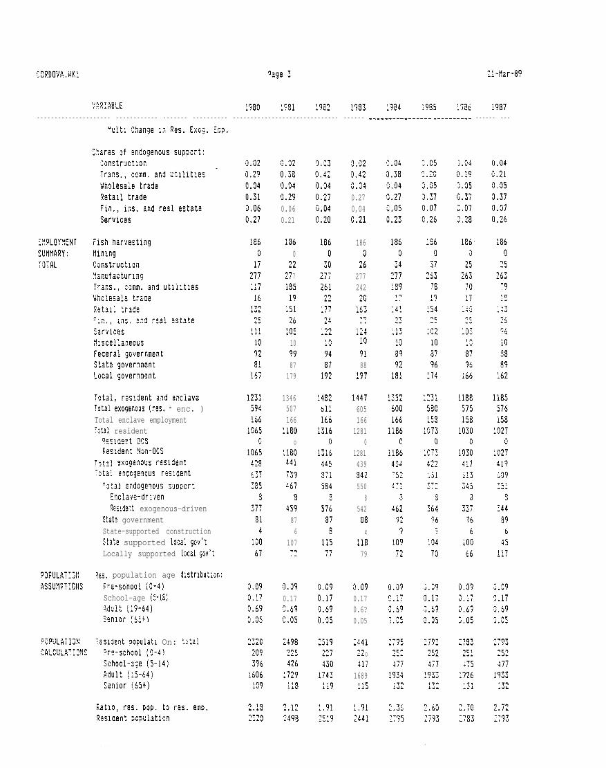
‘/C,~~~~~E :980 :?31 ..8-*q ~ !783 :7i!4 ;935 1986 :787

- - - - - - - - - - - - - - - - - - - - - - - - - - - - - - - - - - - - - - - - - - - - - - - - - - - - - - - - - - - - - - - - - - - - - - - - - - - - - - - - - - - - - - --..------------ .--------- - - - - - - - - -

estate

wclaveTotal exogerious (res. + enc. )Total enclave employment:otai resident

Reslwr!t Ocs!eslde~~ !/~n-o~S

T~!~] :~ogenou: r:sldefl:‘~ta! ~n~cgefiou~ ~~~~de~t

‘O:al ~ndogenous j~~portEnclave-dr:’/enResident exogenous-driven

State governmentState-supported constructionState supported local gw’tLocally supported lociil gov’t

?2s. population age d]strlbution:?re-school (0-4)School-age (5-18)Adult {19-64)S:nlor {$~+i

?: Sldl?Pt 90pUlati On: 5Jhl

0.020.3s0,04!),290.060.21

1960

22e-lLI 7185la

!519.6

:0510w87

179

1346507166

!180o

:!804417;9467

9459876

107;?

1.090.17?.69C.05

2498‘7’?C.,-4

426!729,{~Aiu

2.122498

8.020.42:.!)40.270,04C,21

1860

26277242

2C!63“y. .

124JOq~88

!97

1447605166

12810

1281439342550

8542w

1

11879

2.090.170.6?0.05

:441?5LL o1;:

1689Ilc.LJ

1.91

2441

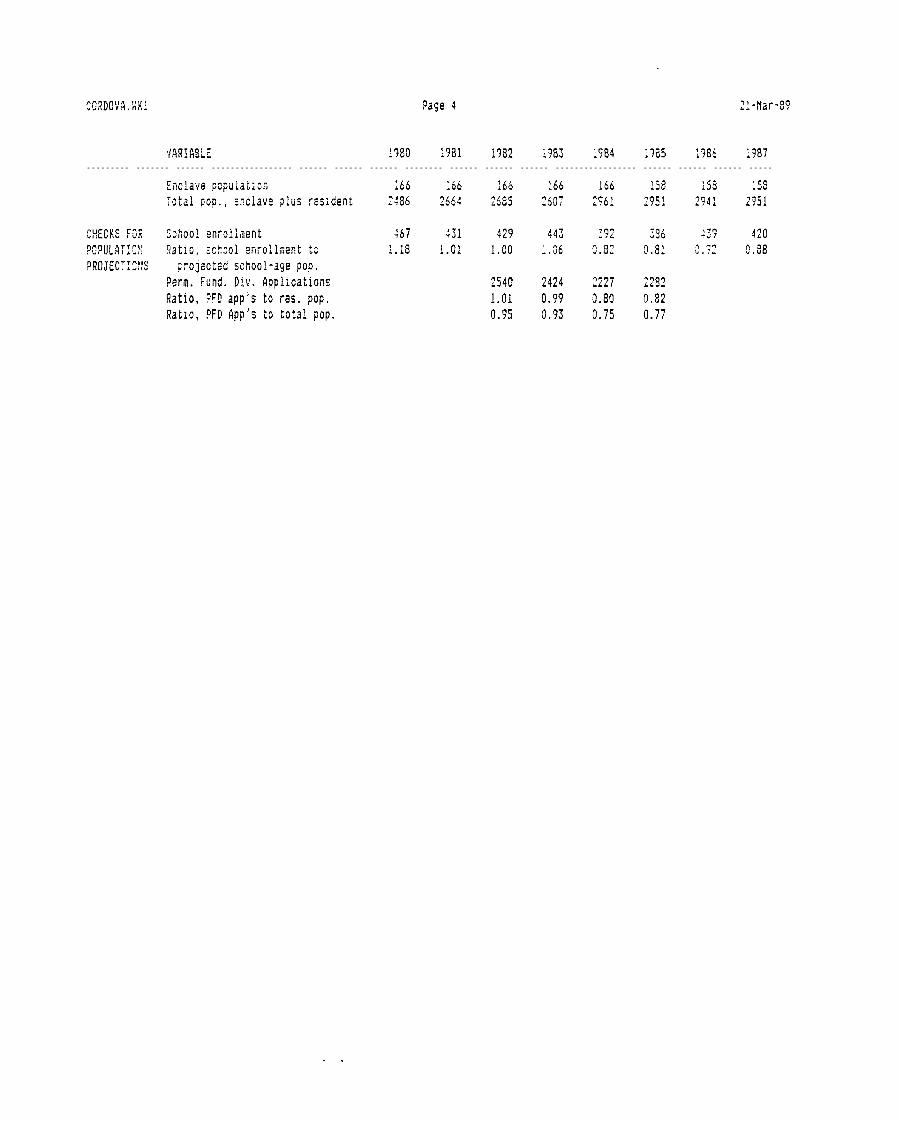
‘lFNIfiEiL: i?eo :991 1982 :?8ZI :984 :7’55 i985 :987

- - - - - - - - - - - - - - - - - - - - - - - - - - - - - - - - - - - - - - - - - - - - - - - - - - - - - - - - - - - - - - - - - - - - - - - - - - - - - - - - - - - - - - - - - - - - - - - - - - - - - - - - - - - - - - - - - - - - - - - - - - -

.,

r ,,IIII#II,1II:1IIItI1

‘20cclco

--4 . . .

C3-a(nT0- ’m

c-l.->,-_

mx0-!

,

IIIiII

mxl-.

“m

L-I-n

06., -. . .4. 4 u-4 ,-- G-. F..z.-l.>l-n.n

0000 --- -!-. . . .I.-; -- UILIOOO :>0000000 0<20<> 0+-0 0. . . . .L- L- ObOO 00.-Daooaoa 0

b-.(3w0

,.- 0. . ,.>-- v C..4 r..> coD. CA O. QPJ*- .Pa.>a>miI . .c-> L,, ..-. . C, CC.’JI

cr. .$- r’, til m)--cD.t.. m.m

0000 .-,- ,-, . .. . . . . . . .-b.-t.rlulc=. o 0=Oaaoooo c>

U’>c.>u t---u <>. . . . .● - - . . L C > > 3 0 > 3 O aOoaooooo0

III<> .4 $.-. . cd -4 ,.,

c- L-4 .- a l.,0 ..3 r.~ c> co

0 0 <.> ‘:-> -— .–. t-- ). . . . . . . .I--)-- clllmomo c>c.000000.3 <2

,.:, <> <> I_> $-- --- u a. .;-- ; -- >D.aoi>o.o..~c>ooooo 0

C2 L.1 s. . [ ., t.” L,,W- Ln C.-1 4 L,4(.4 u. - t. r.1Oc>oc> e,- -.. ,.,OO’., + .-00. . . . . .L- LLt;m OOo k wLca LOOO 00000000 c> Oc>clJaaoo 00

C2

‘.>

,>

b-. c> ,-.- 0>” P.> m

cr. C.4 * - C-I r.~ <> u c:, CJ m

a > ’ 4 # -. . ‘ . , !,, ‘,!0’. “.c,lca ..1r... L.J c .1 m cm

.- .-->,–. a -k ,.Lo, ,. CA -- co <..1 : ; <> C3 c>. > u.

‘-) (.1... . . ., ..,,, ,LIIL-J, -.- JI. Ico ● - [.4 <0 (.0

i , .>,-:Xr.>-1

II - - -

. .3I .GOuc>cs.c .>’ >’.> ’.>lm,

‘,, ;,,3’->1. }- C.>C>. . . . . . . .*-, --am a’-*o 0C>vc>oooa 0._) ’,... . c4cla8,me. . . ,---.4& !--- {m ,7. -?1

{.:1. n

Page b

Nholesale trade (Sridogenow)

?~rvl~~:Resident exogenousResidwt, .wdogenow support

Exogenous share

~$,~~L!~~TI~)j ‘;~~ 1 :ndogefious support!Constructlon

7: EHD13GENOUS ‘rans. , comm. and Ut; lltie S

~~?poRT Hiolesale tradeE!IPLCY!!ENT ?etail trade

F,‘In. , irs, and real estate$erwces

Generated by:Enclave employment

Endogenous suppOrt &TDIOY!nenCgenerated per enclave employee

?esident exogenous driven

Y!4RIA8LE 1958 ;989 :990 lpQl :792 !993 1994 1995--------------- -------- ---------- ------- -------------- ------------ --------------------- ------------------ -----.-----.-.--

!iult: C!iarige in Res. ExOg. E~9.

Shares of endogenous support:tcnstructionTrans. , ccflm. arid utilikie~l’lho!esale trade!i’etall tradeFin. , ~ns, and real estateServices

EIIPLOYHENT “?ish harvestingSUIIMARY: XlnlngTOTAL ‘Construction

Manufacturing:r;ns. , WM. and utllltles

MLCUL9TIONS ?re-sc~~ol (o-i)School-age (5-14)&wiE fi5-64jSenior (65+)

?2tlo, res. pop. to~eslaent population

1.00

0,040.210.050.370.070.26

1860

232631918

:43?696103877

156

1164516158

10070

1007419538552

El344774

:9!17

0.090.17G.690.05

2739247467

1896129

2.722739

;.00

0.040.2]0.050.370.070.26

1860

2126379:9

;4425?~109869

152

1152571158995

079541’7575;~~

234;699

:;117

j.~90,172.690.05

?706244462

1873127

2.722706

!.90

3.040.212.050.37:9.070,26

;a6

o22

26330!8

:45-:. .,7c108812

!54

1159578!55

iO02o

:002420X2?:7..”

1.:4572J

7~ 7!!7.4,

,J,og0.170.699.05

2725245465

1886128

?,722725

:.01

0,040,21i).o~0.370,070.26

lEi6o

22263!3018

1 ‘K~f-c77109870

1s3

1158578158

10010

1001$21Wgw:

o34;70

7d

36:17

2,090.179.69~,()~

2722245465

1884128

2.722722

Page 8 21-flar-8Q

VHRIMLE 1988 1989 ~99f) 1991 i992 1?93 :794 1995-------..---------------- --------------------- ---------------------- --------- --------------- .--.-------- -----------------

Enclave population 158 !58 158 158 158 :58 ;58 !58Total PO D.) enclave DIUS rwdent 2396 .G6+.0 7 2883 2879 2899 2?ol 2837 2918

CHECKS FOR Scnool enrollment 429PO? ULIITI!JN !7atlo, school enrollment to 0.92PROJECTIONS projected school-age pop,

Perm. Fund. Oiv. applicationsRatio, ?FD app’s to res. pop.Ratio, PFD flpp’s to total pop,

Retail tradeC:n. , Ins, andServices

~]~CL~yfl~YT Cish harvestingslVl!l!lRY: ?!Inlng‘2!IIL tonstructlon

Manufacturing

real estate

~otal, Tesldent and encl~yeTotal exogenous (res. + enc. )Total enclave employmentTotal resident

Res~dent ~C$Resident Non-OC$

‘oh! wogenws resident73:31 ?w.logenous rwlden!

‘ctal endogenous 5UpDOrt

Enclave-dr:Yen%sldent ?xogenous-drlvec

5:2t. e Sovernrnent$:ate-supportes construc:l~:,State s2PGorted local gov’tLocal!y sumorted local gov’t

PCPULATICN :esiilent population: tOtal“;! LCULflTIDNS ?re-school (C-4)

$chcol-age !5-:4)fidult (15-64)Senior (65+)

!latlo, res. pop. to res. emp.Resident pop~l~~ion

:,02

0,040.210.050.370,070.26

!86o

22?53

164583158007

0ioo7

:.02

9,04~,~19,050.370,070.26

1960

22263

:,09 :.0?~.i7 0,17:.59 :.5?:1. C5 0.C5

li70598i58

10!30

:.03

:.04o.~10.050.37:3.07g.~~

1860

2226334:9

,:.. . tl.1-?

102108868154

i177589158

,Cll. . . 90

r>[xl ,-.4 ‘.u. cc,

e,. 0 . .C-4 mco c “

I11,iI#

,I

1

I11

I

iI1

i1I

,,!II

:I1I

iI

1

I1> ,“3*-,Lflt-nlam i

1

#r, ,.0 >- ,C4 L,. I4- ccl ,

1)

ir> ,. , 3 , . ,r.> L/l 1* . C,CJ i

I

c,.,> * -t- 1...r.1 co

r.>.s3, -CJ L.n*- ccl

I1

II

tI

I1

i

1

--Dw

.%r-m

r J,-

4Cu-,

CL.0

;ORD9’;#. ii: ?age 13 11-t!ii-g5

-------------- ;: : ------------------ ----------------------- -----:.--_ ----------- ~ ----------------- ;,----------------- ~:::-,#RIA9LE ~oo4 -305 ~oo6 .0C7 mgs 4J09 ~~1~ -J*J

OcsEllPLOYl104TRESIDENTSHARE

Offshore long-term skilledOffshore long-term non-ski.

Onshore short-term skilledOnshore short-term non-skiOnshore long-term skilled

led

led

‘;,! R!ABL: :!294 ~o::, -+.fl200L :2:7 -Jd

. - - - - - - - - - - - - - - - - - - - - - - - - - - - - - - - - - - - - - - - - - - - - - - - - - - - - - - - - - - - - - - - - - - - - - - - - - - - - - - - - - - - - - - - - - - - - -

::T?. . .

!Il. “

:’xjg :::~ 2011------------------------

,7C---

.,

.-,-.

.;..<:. . . .

-{.,, -

:,,b 1

.l~7L;.

.r

. . .

,:.

- - -

- <fin,. -W.

r,

. .. -.,c

-?,,

“2. :92

. .. .

. .,

. .

‘. ‘,,. :

..-.

.-,

. . .

,:----

,-, k c. . . .

0

Co;

;!!/1!5:: 2004 2005 2006 7807 2008 ::~? :~lo :011.---------- ----------------------- -------------- ------ ----.--- -------.------.-------- --------- --.----------- -------------

W3WL8TICN ?es. ?opulation age qlstributlon:lSSUH?TIC!;S :re-scfi(lol (0-4)

School-ase (5-18)&dult :19-54)~~ilio~ (65+)

Ritic, res, pep, to rest emp.?esldent population

In3. . .

0.040.219.050.370.07o,~6

!~6o

~~26384;?

;5727:02108865153

1175591158

10180

1018~j~

5:5

3633

256653

;3120

0.090.173.69J.05

2768249472

1916130

?.722768

1.04

0.040,212.050.370.070.26

~~6

o‘?2

26385!9

:?:

27:03108864152

1175592!58

:0170

!017434583164

855654TJ

:2!20

0.09om170.69~do5

2767249472

i915i30

2.722767

:.34

C.J4n n!U.LL0.050.370.073m~6

!Bbo

22263g~;0

:~qp

:03iO8861151

~!74

593158

iO16o

1916435:81Z65

8;57613

31120

0.090.17$.69~,~ 5

2764249412

191313(I

2,722764

!.04

‘3.040,212.050.370,070.26

1860

222658519

:;;~?

:0418SE60

15 1

i174594iz~

!016o

Iglb437580;66

825860:

31!~~

2.09QO:?J,69:,05

2764249472

1913130

2.722764

‘iARIA8LE 2004 2005 2006 2007 2009 2’209 2010 ;011------ ------- ------------- ------ -------- -------------- ------ ------ -------- --------.--.----- ------.-----. ------.-----.--- -

Enclave population i58 158 158 ;5 8 c 8 :58 ;53 ;58Total POD, , enclave plus resident ~925 ~w~ 2922 2922 ;ijl ~~~~ 2944 2’752

CHECKS FOR School enrollment~OplJL8T10~ Ratio, school enrol!inent to?R(JJ~~T1~}~S projected school-age pop.

Perm. Fund. Div. Applications

Ratio, ?FD app’s to res. pGp.

Ratio, ?FD 9PP’S to total pop,

VARIABLI 2012 2013 2314 2015 2016 2017 2018 2o19------ -------------- ------ -------- ------- ----------------- ------ ------ ------ ------ ------------- --------.---- ---------- ----

~oshors short-tern skl!ledUnshor? short-term non-skliledOnshore lcng-term skilledOnshore lcng-wrn noci-skilledOffshore snort-term ~klll:~Offshore short-tern non-skilledOffshore long-term skilledOffshore long-term non-skilled

Onshore short-term skilledOnshore short-term non-skilledOnshore long-term jkllledSnshore long-term non-skilledOffshore snort-tsrm skilledOffshore short-term non-skilledoffshore long-tern skilledgffshor? long-ten non-skilled

lnsnore short-tsrm willedOnshore ShOrt-terM ncn%kllledOnshore long-term WilledOnshore long-tsrm non-skilledgffsh~re short-term skllled

Offshore short-term non-skilledOf%hors !ong-tern skl!ledOffshore long-ter~ non-skl!led

C2nstrcctlon: total:i-!coss Generatea kY state spend]ng

%tlo Gf ;t. PC ?XD, to ’87Ratio of tot. ex, em. to ’87

EodogenousEndogenous share

ExogenousExogenous share

JcL-,

3

c

j

~

o

0.000.00!.00i.oo0.000.00O.!()(1 ~U.L o

!.30:,0!)1.00;.000.500.500.100,10

5

ii’i:’24]::2?J:

0.49

!86

nvo~Q

;T.

9.411.04

i3

6

03‘2o0000

0.00~,oo!.001.000.000.000.10‘1 !0V.L

:.00.n. . .0!.00:.000.500,50C.io2.iO

c

i91:741:42

2.813.49

185

~:

‘)~

97“

0.41~#’J~

13

5

00cJ

o000

0.000.00!.001.000,003.009,10:.lC

:,~g‘nc

i.00,3i.u o0.500.500.10~.~o

o

G;l:’74!:J:

:03~;,49

1%

o010

y7.

8.41i.05

13

6

I

11118

I

I

I1I

1

1II,I

b1

i11I1II

L,>.. :::>

,,xLO

wuc.

J1,), -.(1,(0.10,.+m

-..CD:.,

c1

./

N

, .,c o

,.><;>

h>w

1>[0

t .,L-O

,,u

,. ,< .“

-4—m

y, :’

‘., !-,0 D,<1> +-11>c n(!> .

:-1<t>> :

,-. 1-,‘, -

I

I

- !.*10 r>- J

a---J

-.*-Co [> CcJ- . ,

m--4

0

“0.5-..IW.F-acOlw

--- Q *—. . . ,.-,—L.> 0. 1..4 0 N tn

c> -r- (.. *- .s- t..a t-l

t-- ,.:). .CJ 0. ‘P.$- &”+--

+. D.-.C-4C.,4U.0 . 0 0 .

CA

-P.

r .1u.

< 4

cr.

c .1u.

‘.,c-.4

c.,--J

c . . .--4r. .3

cl-.,r - d

,- ‘4u} FJ CA - . . . *— -4c7. lDG-. a.3fAN

,-.aWoG- a - - l

i.=)

I r>g :,; >:; :,: , c,

,#-.OOcu Lrlcll L-I

I

,.<>. .c, cr. cr..b-Ln k--

,- <..1.431. >C.I. -C,,I-. -.!--.lcO--J.0mlAc.l

.-.L

F-J>( > u. ,7-.

L., L,, , . . .

,-+CA . . 4 0.--! b.> a

,-.43 ,.- m+-m

#0,.<>

‘3 & <f.[n ( “ ---

,- <.-4.0 12 C.I t-- co - -4-4c0-.I.0c2ulJl

.-.0-0--4 w m

, - ,...C-4 ,.4 .-d--4 CA 0

Ococa-04”3

0

L0 ‘x,4-O.4G

---- (7 t -. . . , - ,.-a u-. t., <> ,.2 m

<> ‘J-1 ‘/7 *- ‘.” C.I .r-

,-0. .‘.> m ‘,.1“ ,,1 , .

.0,- .-=.cm ,- ,0

. . .22

,-<>

*-c)

, .-<>

I:> I

wG ! . --- r..> :0OLn Ore.,-

aOcou-tr,l l-4

I

..<, ,.- -C.i <>, --Icc) ‘m L-i

.0 , *--031.0

<.> .,. <,.c. <“ -

0

!--Ocol-. oQ- 0,--

.> i1 ‘.,

4-1. .,.>10OLIlc> u.,---

taala, ,,c .1, co1I

}-,-.>}-. . . l. ..,--

U u. <., ‘> P> L.n‘., CI.U-l, -13. L., Lrl

..<>. .C, U. L..cr. [r! - - -

“> -.43 ,- *-ml...-=!

,---C.4 {.., d.s 0. C.n

, c.>. .,.> c,. (-,.

‘ t . .>, r.,

, --+ ,.. ,-.ar, l-

,— .-L-4 , . . , -.-(.0 -.I r.

“ARIABLE--------------: ------------------- -------------------:: ::-----:; : ------: --------: --------:: -------::: ~-----:’: _------: ----3 ’014 “01s ‘“16 ‘“i E -019

;Jho!esale trade?eta:l trade:,n,, Ins. ana real5ervlces!!lscellaneousFederal governmentState governmentLocal government

Total, resident mt

:t!j 6

0.040.210.050,370.070,26

18609

2638819

16628

107lo8861

;52

1188601158

10310

1031;JJW7~: 2

0

36;’Al7

3;!~~

0.090.179.690,05

28032!53410

1940i32

2.722803

Inl,U 6

9.040.210,050.370.070.26

1860‘1

?538819

:67 ‘28

:07103861

153

!191502158

:0240

:034:455~7777.,, U

3-365$17.

71&

;i~q(1.!?2.690.05

2s12252480

1’746132

2.722812

:.37

0.040.210.050s370.070.26

!86o3

:638919

:6928

:08108861

:53 .

1195604’158

:0370

1037i~.jCrll-,, ,~-.; 4

~

zi 661J

3!!~~

0.090.170.693.05

:8Z1254Ai3~

~952133

2.722821

i.07

2,040.210.050.370.070.26

18609

2638919

170~g

:08108861154

1198505158

:0400

:C40448593::~

8568617.

31!~~

:,090.179.690.05

2830w~

4831959133

?.722830

cc RDova. iKl Page 20 2i-!lar-89

‘I! R188LE ~ol? 20i3 2014------------------------- -------------------- --. ----. - 1. -:----------- ------------: --.-. . .--:-------- :-------.::: -.----:!:--

~ols “016 ’017 El 9

- -Cnciave pOpuiation ! yJ 15s 1:8 i~~ . .~~: ‘8&- :53 ‘81:Total pop. , enclave plus resident 2%: 2’769 2978 2X37 :q97 ~c~~ ~’;ib 3027

CHECKS FOR School enroilnentWPUL9TION Ratio, s~hool efirollfient toO~oJECTIoN~ projected school-age pop,

Perm. Fund. Div. Applications

Ratio, ?FD app’s to res, p o p ,

Ratio, PFD APp’j to ti)t~l pop.

I/qRI~~~~ 2020--------- ------ -------- ------------------- -------.--------3:S

EHPLOY!!ENTTOTALS

OcsEMPLOY!!ENTRESIDENTSHIIRE

OcsEMPL9’I!IE?+TENCLflVESHARE

OTHER OCSASSUMPTIONS

STATE ‘W’TPER CAPIT;SpEyDING9SSUMPT12NS

EIWLOY!!EN?

ilnshor~ short-term ~k.~ll~t‘lashore skort-tsrin non-skilledOnshore long -terfi sl. illsdCnshorE long-tern fiun-skllladOffshore short-tern skilledCffshore short-term non-skllleaOffshore long-term SkilledOffshore lG.ng-term con-skilled

Onshore short-term skilledOnshors short-term non-skilledOnshore !ong-tern skilledOnshore lcng-!erm non-skilledOffshore short-term sklllsdOffshore short-tern non-skl!ledOffshore long-term Skilled~ff~h~r: ~,~ng-i~rn fiOn-~Kl~]2d

~nshors siwrt-ter! skilledOnshore short-term non-skilledOnshore long-tern skilledOnshore !ong-ter,m non-skilledOffshore short-term skilledOffshore short-term non-skilledOffshore long-tErm skilledOffshore long-term non-skilled

Local government employmentsupported by OCS revenues

Fish harvesting (reslden:)CALCULATIONS

!lining: totalNon-0C5 resident (exog, )WS resident (wog, )OCS enclave

C0nstr3ction: totalE!ICOSS Wnerated by sht~ spenjlng

!?at. io Jf s:. PC W. t; ‘elRatio of tot. ex. sm. to ’97

EndogecousEndogenous share

Exogencus~xogen~us share

o9000003

0.000,001,001.000.000.000.10;1.10

1.001.001.001.000.500.50o.!rJ0,10

0

6914,IQ I./

:4???1_.b

0,49

196

,2,1,-

;

0

Q

30.41!.06

!4

L“

-. . . . . . ., -.. . . . . . .

WRDOVR. !JK1 %ge 22

Va91.48LE 2020. --------------------- ------ ------------------------------

Hanufacturlncj: total~:~ident :Ish processliig {e:{O?.)

:flclave f:j!l prccmifi:

Residmt s;,are

OLhw Ranufacturlns

?rafis, , comm. and uiiliti:sResident exogencus!iesidmt, &ndogenous supportExogenous share

!iholesale trade (endogsnous)

Retail tradeResident exogenousResident, endogwms siJp?ortUogenous :har:

Cir,., ,,, ifi~. and reai estate (er?d. ~

:ervicssResident exogenousResident, endogenous wpportExogenous share

?liscellaneous (exog, )

Federal government (exog. )

State governmentRatio of st. PC op. w, !,6 ’37Rat]o of tot. 2x. efi. to ’37

Local government

Supported by local revenues!latio of tot. 2x. em. to ’87

Supported by ztate spendingRatio of st. PC op. exp. t.o ’87Ratio of tot. :x. em, to ‘S?

Supported by OCS revenuesMare supported by state

C#LCWHV4 Total endcgenous supportconstruction

qF Ef~~(jGE~O~S ~~aiij., comm. and utilitiesSUPPORT lholesale tradeCM PLOWEYTL!! Retail trade

Fin. , Ins. and real estate~e~vice~

Generated by:Enclave employment

~ndogenous sup?ork, Snploymentgenerated per enclave employee

?esld~nt exogenous driven

21-flar-89

CORDOVA.lK1 ?age 2:

‘VARIASLE 2020----------- ----------- ----------- --------- ------ ------ ----

!ult: Change in Res. Excg, Ew.

Shares of ?fidogenous support:ConstructionTrans. , comm. and ~t.illt.ies

Iholesale tradeRetail tradeFin., ins. and reel estateSerwces

EMPLOYMENT Fish harve~tlngSUflM!!R’f : MiningTOTAL Construction

!lanufacturingTrans, , mm. and utilit. i%IIholesale tradeQ~t~il trade~:!~., lilj, JCd real SstateWvlczstilscellarwusFederal governmentState governmentLocal government

Total, resident and enclaveTotal exogenous (res. + enc. )Total enclave employmentTotal resident

Re$ldent OCSResident Non-OCS

‘<3tal exogenous res:deritTotal w!ogenous resident

TO~al ~ndOgenOUS support

Enclave-drivenResident exogenous-driven

State government,State-supported constructionState supported local gov’tLocally supported

OIJplJLflT1iJN %s. population age9SSUtlPTIDh’S Jre-school (O-4)

School-age (5-18)Adult (19-64)Senior (65+)

POPULATION 7esldent populationCALCUL8T19NS Pre-school (O-4)

School-age (5-14)fidult (15-64)Senior (65+)

Ratio, res. pop, to?esident population

local gov’t

dl~trlbution:

total

res. emp.

1.09

0.04ol~l0,050.370.070.26

18609

2639220

l-l~; a28

112108862

156

1216614158

10590

1059456$03382

“

37;6?3

32124

0.090,170.690.05

2S80259491

1993136

2.722880

.

21-llar-i!Q

*

COR!)OYA. XK1 ?aqe 24

‘J9RIPJ3LE Z020. ----- ------ ------------------- -------- -------- -----------

Enclave population 158Total pop, , enclave plus resident 3037

Ct!EC!4S FOR School enrollment!JOPULilTION Ratio, school enrollment toPROJECTIONS projected school-age pop,

Perm. Fund. Div. applicationsRatio, PFD app’s to res. pop.Ratio, PFD App]s to total pop.

2i-!lar-89

.

As the Nation’s principal conservationagency, the Department of the Interiorhas responsibility for most of our nation-ally owned public lands and naturalresources. This includes fostering thewisest use of our land and water re-sources, protecting our fish and wildlife,preserving the environmental and cul-tural values of our national parks andhistorical places, and providing for theenjoyment of life through outdoor recrea-tion. The Department assesses our en-ergy and mineral resources and worksto assure that their development is in thebest interest of all our people. The De-partment also has a major responsibilityfor American Indian reservation com-munities and for people who live in IslandTerritories under U.S. Administration.